Fault location on transmission and distribution lines A ...
34
CALIFORNIA STATE UNIVERSITY, NORTHRIDGE Fault location on transmission and distribution lines A graduate project submitted in fulfillment of the requirements for the degree of Master of Science in Electrical Engineering By Roshan Lakde MAY 2013
Transcript of Fault location on transmission and distribution lines A ...

CALIFORNIA STATE UNIVERSITY, NORTHRIDGE
Fault location on transmission and distribution lines
A graduate project submitted in fulfillment of the requirements
for the degree of Master of Science in
Electrical Engineering
By
Roshan Lakde
MAY 2013

ii
The graduate project of Roshan Lakde is approved:
____________________________________ _________________
Dr. Ali Amini Date
_____________________________________ _________________
Dr.Nagwa Bekir Date
_____________________________________ _________________
Dr. Bruno Osorno, Chair Date
California State University, Northridge

iii
Acknowledgement
I want to thank many great people who helped me and supported me during this project.
I would like to express my sincere gratitude towards Dr. Bruno Osorno for his guidance
and consistent supervision. He has taken pain to go through the project and make the
necessary correction when needed. I feel privileged to have him as my guide and
supervisor as well.
I express my appreciation to Dr. Ali Amini and Dr. Nagwa Bekir whose knowledge,
support, encouragement made this study successful.
I would like to express my gratitude towards the most important people in this world to
me, my parents, for their moral support and motivation; without which I wouldn’t be who
I am.

iv
TABLE OF CONTENTS
Signature Page………………….…………………………………………………………ii
Acknowledgment…………...…………………………………………………………….iii
List of Figures…………………………………………………………………………….vi
List of Tables…………………………………………………………………………….vii
Abstract………………………………………………………………………………….viii
1. Fault location
1.1 Introduction ……………………………………………………………………… 1
1.2 General division of fault location techniques …………………………………… 2
1.3 Input signal of fault locators …………………………………………………….. 3
1.4 Factors influencing fault location accuracy ……………………………………... 3
2. Traveling wave technique
2.1 What is traveling wave? ……………………………………………….………… 4
2.2 Benefits ………………………………………………………………………….. 4
2.3 Theory …………………………………………………………………………… 4
3. Single ended method
3.1 Factors which affects the fault location calculation ……………………………... 6
3.2 Equipment and the input data required .…...…………………………………….. 7
3.3 Fault resistance and load ……………………………………………...……….... 7
3.4 Different single end method algorithms ………………………………………… 9
4. Double ended method
4.1 Equipment and the input data required ……………………………….………. 12
4.2 Common approach/ Algorithm ……………………………………………...… 12
4.3 Algorithm used for Matlab …………………………………………….…….… 13
5. Fault location on distribution lines
5.1 Introduction …………………………………………………………….………. 16
5.2 Different approaches …………………………………………………………… 16
5.3 Conclusion ……………………………………………………………………... 19
6. Fault location MATLAB simulation…………………………………………………. 20

v
7. Conclusion…………………………………………………………………………… 24
References………………………………………………………………………………. 25

vi
List of Figures
Fig 2.1 Traveling voltage and current waves ……………………………………….…… 4
Fig 3.1 One line and equivalent circuit for a 3 phase transmission line fault …………… 7
Fig 3.2 Fault resistance of fault resistance and pre fault load errors ……………………. 8
Fig 3.3 Single line diagram form single ended fault location…………………………... 10
Fig 4.1 One line diagram and equivalent circuit for fault on line ……………………… 13
Fig 4.2 Single line to ground fault condition …………………………………………... 14
Fig 4.3 Network connection seen from substation A …………………………………... 14
Fig 4.4 Network connection seen from substation B …………………………………... 14
Fig 3.3 Single line diagram form one ended fault location……………………………... 20
Fig 6.1 Transmission line Schematic using Matlab/Simulink………………………….. 21
Fig 6.2 Transmission line model with fault location calculation single ended method… 21
Fig 6.3 Single line diagram form one ended fault location single ended method ……... 22
Fig 6.4 Transmission line Schematic using Matlab/Simulink for duble ended method .. 22
Fig 6.5 Transmission line model with fault location cal. for duble ended method……... 22
Fig. 6.6 Transmission line model with fault location cal. for double ended method…… 22

vii
List of Tables
Table 3.1 Equations for simple impedance ..………………………………..…………... 6
Table 6.1 Parameters of the line used for analysis ……………………………………... 20
Table 6.2 Results and % error for Matlab analysis …...………………………………... 23

viii
ABSTRACT
FAULT LOCATION ON TRANSMISSION AND DISTRIBUTION LINE
By
Roshan Lakde
Master of Science in Electrical Engineering
Fault location is one of the most critical issues of utilities and electrical companies in
today’s competitive market. Analysis of fault location not only ensures the continuous
power supply but also help to study properties and weakness of particular power network.
In the following paper, I have discussed various traditional and new approaches to fault
location. Also I have done Matlab simulation to prove the accuracy of the algorithm. I
have used fundamental frequency component of fault voltage and current for the analysis.

1
1. Fault location
1.1 Introduction
Fault location is a procedure projected at locating the occurred fault with the highest
possible accuracy. A fault locator is mostly additional protection equipment, which apply
the fault-location algorithms for assessing the distance to the fault. [1]
A fault-location function can be implemented into:
• Microprocessor-based protective relays;
• Digital fault recorders (DFRs);
• Separate fault locators;
• Post-fault examination programs.[4]
“Protective relays are narrowly correlated with fault locators; however, there are some
alterations between them which can be considered as related to the following features
Correctness of fault location;
Speed of defining the fault position;
Speed of spreading data from the remote site;
Used data window;
Digital filtering of input signals and difficulty of calculations.”[1]
“Fault locators are used for identifying the fault position correctly and not only for
warning for the general area (defined by a protective zone) where a fault occurred which
is the case for protective relays.” One of the crucial requirements imposed on the
protective relays is speed of operation. The faulted line has to be cut off from the main
grid as soon as possible to prevent the spreading of fault effect. “Therefore, high-speed
measuring algorithms are applied in contemporary protective relays. The use of high-
speed operating circuit breakers is also of prime importance. Fault-clearing time is an
important consideration in the selection of protective relays and requirements for relaying
speed must be determined carefully. System instability, excessive equipment damage,
and adverse effects on customer service may result, if the relaying is too slow. While
faster protection will lead to negotiate relay system security and selectivity.” “The
requirement for the fast clearing of faults demands that the decision for tripping
transmission lines has to be made in a short time, even faster than in one cycle of the
fundamental frequency (for the systems operating at 50 Hz it will be 20ms). On the other
side, the analysis of fault locators are performed in an off-line mode since the results of
these calculations (the position of the fault and in the case of some algorithms also the
involved fault resistance) are for human users. This implies that the fault-location and
speed of calculations can be measured in seconds or even minutes. Low-speed data
communications or supervisory control and data acquisition (SCADA) can be applied for
fault-location purposes, which differ from communication used by protective relays. The
best data window segment from the whole available window can be selected for the fault
location to reduce errors. This is so since the computations are performed in an off-line

2
regime and searching for the best data window can be easily applied.” The fault interval
lasts from fault incipience up to a fault clearing by a circuit breaker, and usually this
takes around three fundamental frequency cycles, which is wider than required for the
fault location. In the case of the protective relays the required high speed imposes that
applied calculations should not be too complex and too time consuming. In contrast,
fault-location calculations do not have such limitations. As for example, rejection of DC
components can be applied for more accurate phasor analysis of the fault location. Also,
models of power lines and faults in fault-location algorithms are usually more advanced
than the computational capacity of microprocessor relay. Among different types of relays
commonly used for protecting power lines, distance relays are the most related to fault
locators.“When fault is identified as occurring within the pre-defined protective zone,
then a trip signal to the corresponding circuit breaker is sent immediately. In
consequence, the fault becomes isolated quickly, which minimizes the impact of a fault
on a power network. Distance relays have multiple protection zones to provide back
capability. The relay that detects the fault in the 1st-zone is designed to trip first.
Generally, a pair of distance relays is used to protect a two-terminal line. Usually, they
communicate among them, creating a pilot relaying. As a result of exchanging
information between the distance relays from the line terminals, they both could trip at
the 1st-zone setting. Operation of a distance relay may be significantly influenced by the
combined effect of fault resistance with load, which is also called as the reactance effect.
The distance relay may mis-operate for a forward external fault, or may not operate for an
internal fault if the value of the fault resistance is too large. The value of the fault
resistance may be particularly large for ground faults, which are the most frequent faults
on overhead lines.”[1][4][5][6].
1.2 General Division of Fault-location Techniques
Fault location is possible in a natural way by foot patrols or by tech persons equipped
with different conveyance means and binoculars. These means of faulted-line inspection
is considered as time consuming. The method of fault location involved optical
inspection as is mentioned. Also, calls from witnesses of harms on the power line, or
client calls, can deliver the required knowledge about the fault position. However, such
simple ways do not fulfill the necessities imposed on fault location [2]. Valued
information on fault location can be gotten also from fault indicators; they are installed
either in substations or on poles (or towers) along the transmission or distribution line.
Additional use of a radio link allows use of the info from indicators also during bad
weather. In spite of several efforts to dissimilar unusual techniques, automatic fault
location is still famous and most widely used. It is based on determining the physical
location of a fault by analyzing the voltage and current waveform values. Automatic fault
location can be classified into the following main categories:
• “fundamental-frequency of currents and voltages, impedance measurement”
• “traveling-wave”
• “high-frequency components generated by faults” [2][3][6]

3
1.3 Input Signals of Fault Locators
Mostly, the fault voltage and current are used for the fault location. However, pre-fault
quantities may also be used in many fault-location approaches. But usage of the pre-fault
data is treated as the drawback of the fault-location technique. [2][3][6]
1.4 Influencing factors on Fault-location accuracy
Following are the factors that may influence
“Inaccurate compensation for the reactance effect”
“Inaccurate fault-type (faulted phases) identification”
“Inaccurate line parameters, which do not match the actual parameters.”
“Uncertainty about the line parameters”
“Inaccurate compensation for the mutual effects on the zero-sequence
Components”
“Insufficient accuracy of the line model”
“Presence of shunt reactors and capacitors”
“Load-flow unbalance”
“Errors of current and voltage instrument transformers”

4
2. Traveling wave technique
2.1 What is traveling wave?
“Fault causes transients that propagate along the transmission line as waves. This wave
can have frequencies, ranging from a few kilohertz to several megahertz, having a fast
rising front and a slower decaying tail. They have a propagation velocity and
characteristic impedance and travel near the speed of light away from the fault location
toward line ends.” [7] They continue to travel throughout the power system until they die
due to impedance and reflection waves and new power system equilibrium is reached.
“The location of faults can be precisely time-tagging wave fronts as they cross a known
point typically in substations at line ends. With waves, time tagged to sub microsecond
resolution of 30 m, the fault location accuracy of 300 m can be obtained. Fault location
can then be obtained by multiplying the wave velocity by the time difference in line ends.
This collection and calculation of time data is usually done at a main station. Main station
information polling time should be fast enough for system operator needs”. [7]
2.2 Benefits of Traveling Wave Fault Location
“Uses reflected radar energy to determine the fault location”
“Technique is popular for location of permanent faults on cable sections when the
cable is de-energize”
“Provide algorithm advances that correct for fault resistance and load current
inaccuracies. Line length accuracies of ±5% are typical for single-ended locators
and 1-2% for two-ended locator systems”
“Higher accuracy, Long lines, difficult accessibility lines, high voltage direct
current (HVDC), and series-compensated lines are popular applications”
“Accuracies of <300 meters have been achieved on 500 kV transmission lines
with this technique”
2.3 Traveling Wave Fault Location Theory
ka kb
fault
er1er2
ef
ir1 ir2
e1
i1
2.1 Traveling voltage and current waves

5
The differential equation for a transmission line at any point
………………………. 2.1
where L and C are the inductance and capacitance of the line per unit length. The
resistance is assumed to be negligible. The solutions of these equations are
…………………....……. 2.2
…………......................... 2.3
Where the characteristic impedance of the transmission line and
is the velocity of propagation. [7]

6
3. Single Ended Method
Single ended algorithm calculates the fault location using apparent impedance from one
end to the fault. We need to measure phase to ground voltages and current in every phase
to locate the fault type in this algorithm. If we have only line to line voltages, we can
locate phase to phase faults and if we know zero sequence source impedance, finding the
location of phase to the ground faults is possible.
The following table gives the fault location for different types of fault. Here fault
resistance is assumed to be zero.
Type of fault Impedance equation to calculate the fault
location ( m Z1L)
Ground – phase a VA ( IA + K IR )
Ground – phase a VB ( IB + K IR )
Ground – phase a VC ( IC + K IR )
Phase a – phase b or a – b – ground VAB / IAB
Phase a – phase b or a – b – ground VBC / IBC
Phase a – phase b or a – b – ground VCA / ICA
Phase a – phase b – phase c Any one of above three
Table 3.1 Equations for simple impedance [3]
Where in the above table, K is {[Z0L - Z1L] / 3Z1L } which is the ratio of difference zero
sequence line impedance and positive sequence line impedance to positive sequence line
impedance. Also m is the per unit distance from the fault which is nothing but distance
from fault divided by the total length of the line.
Current and voltage values are used to calculate the impedance of the fault location as
shown in the above table. If we have the value of line impedance per unit, distance in per
unit can be easily calculated. [3][8]
3.1 Factors which affects the fault location calculation
There are many factors which may affect the fault location estimation. Some of them are
as following.
1. Reactance effect, it is combined effect created by load current and fault resistance.
This value is really high in case of ground fault which is actually representing the
majority of the fault types.
2. Wrong fault identification
3. Zero sequence mutual effect

7
4. Uncertainty in zero sequence impedance
5. Line model insufficient accuracy
6. Shunt reactors and capacitors
7. Unbalance load flow
8. Measurement errors
It is important to reduce these factors in order to improve the fault location estimation.
[3][8][9]
3.2 Equipment and the input data required
This method may require the following equipment to abstract the data from a system for
calculation
1. Microprocessor based relays
2. SCADA interface
Following would be the data above instruments provide for the successful estimation
1. Phase to ground voltages and phase current
2. Type of fault occurred
3. Pre fault data may be needed sometime [3]
3.3 Fault resistance and load
Let us consider the simple single line diagram to find out the issues for calculation, the
location of fault using one end data.
Fig 3.1 One line and equivalent ckt for a 3 phase transmission line fault [3]

8
Line between terminals G and H in the above fig is a homogeneous line with an
impedance ZL. RF is the fault resistance. VG and VH and the voltages at the respective
terminal while IG and IH represents the current from the respective ends which will
contribute to the final fault current IF. ZG and ZF would be source impedances.
Voltage drop from terminal G can be expressed as follows
VG = m ZL IG + RF IF …………………………………………….. 3.1
If we divide the above equation by the current IG, we will get the value of impedance
measured at terminal G.
ZFG = ( VG / IG )= m ZL + RF ( IF / IG ) ………………………….. 3.2
ZFG in the above equation is the apparent impedance to the fault which is measured at
terminal G.
The ratio of fault current and current at the fault locator ( IF and IG ) will be a complex
number. Therefore the fault resistance will be impedance with the reactive component in
it. It depends on the angle of the ratio of two current that if the reactive component is
inductive or capacitive. It can be zero, when there is no infeed current from the remote
terminal, or it is in phase with local current.
Fig 3.2 Fault resistance of fault resistance and pre fault load errors [3]
To find out the parameters which affects the angle of IF / IG , we can separate pre-fault
and fault system (Superposition). If IL is pre-fault load current and Δ IG is the difference
or superimposed current then we can write equation 3.2 as

9
………………………………..3. 3
Where ds is the current distribution factor
…………………….3.4
And ns is the current loading factor
………………………..3.5
These two factors will determine the reactive component caused by fault resistance. We
need to reduce the effect of fault resistance RF.
3.4 Different single end method algorithms
Different fault location can be used depending on the circuit data available. Following are
some of them
1. Simple Reactance method
This method assumes that the fault resistance current and current at the measurement side
is in the phase. In this case device will measure the apparent impedance and then will
find the ratio of the measured reactance to the reactance of the entire line.
In this algorithm, fault resistance is compensated by measuring only apparent line
impedances imaginary part.
m = ………………..………………………….3.6
Also for line to ground fault, it would change as follows
......................................3.7
If the fault reactance is zero or IG is in the phase with IF, error will be zero. This
algorithm will give considerable error if the fault has high resistance. [3][8]
10
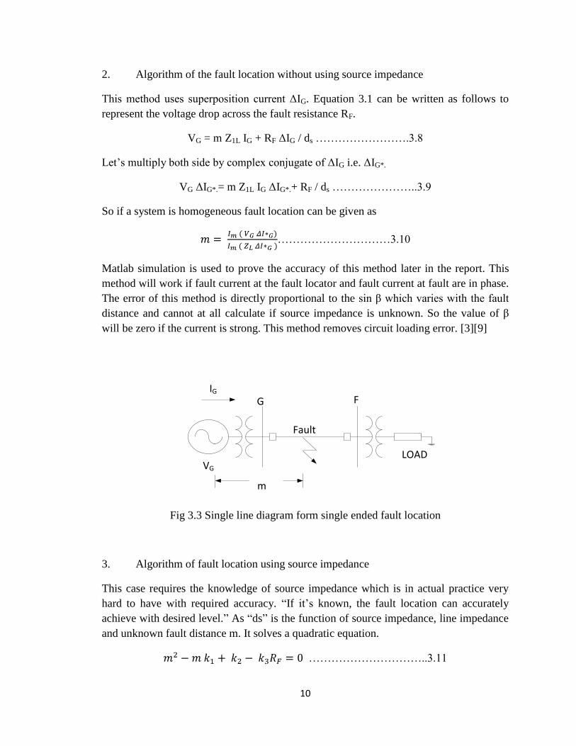
2. Algorithm of the fault location without using source impedance
This method uses superposition current ΔIG. Equation 3.1 can be written as follows to
represent the voltage drop across the fault resistance RF.
VG = m Z1L IG + RF ΔIG / ds …………………….3.8
Let’s multiply both side by complex conjugate of ΔIG i.e. ΔIG*.
VG ΔIG*.= m Z1L IG ΔIG*.+ RF / ds …………………..3.9
So if a system is homogeneous fault location can be given as
…………………………3.10
Matlab simulation is used to prove the accuracy of this method later in the report. This
method will work if fault current at the fault locator and fault current at fault are in phase.
The error of this method is directly proportional to the sin β which varies with the fault
distance and cannot at all calculate if source impedance is unknown. So the value of β
will be zero if the current is strong. This method removes circuit loading error. [3][9]
VG
IG
LOAD
m
Fault
G F
Fig 3.3 Single line diagram form single ended fault location
3. Algorithm of fault location using source impedance
This case requires the knowledge of source impedance which is in actual practice very
hard to have with required accuracy. “If it’s known, the fault location can accurately
achieve with desired level.” As “ds” is the function of source impedance, line impedance
and unknown fault distance m. It solves a quadratic equation.
…………………………..3.11

11
Where k1, k2, k3 are the complex function of local voltage current and source impedance
respectively.
If we separate the above equation in an imaginary and a real part, per unit distance can
be calculated. [3]

12
4. Double Ended Method
Present innovation takes into consideration utilization of information from both ends of
the transmission line. The basic concept of locating faults using double ended method is
similar as that of a single end method. In double ended method, we minimize the effect of
fault resistance and other factors which affect the accuracy of fault location. Fault
location using double ended method is more accurate than single ended method. In
double ended method, we don’t need to recognize the type of fault in order to calculate
the location of the fault. So rather than using zero sequence, we can use +ve sequence
components which minimizes the effect of zero sequence components. The only
drawback is it requires a mean of communication to gather the data of remote end
whereas in the single end method line terminal, relay or devices collecting data is enough.
Double ended method takes more time but it is quick enough to be used by a human. The
response time is in seconds. We must synchronize the collected data from both the ends
before starting analysis. [15][16]
4.1 Equipment and the input data required
Double ended method may require the following equipment to abstract the data from a
system for calculation
1. Any device that gives 3 ph. voltage and current in each phase like Microprocessor
based relays
2. Mode of Communication
3. Data collecting equipment or a tech person at the central site
Following would be the data above instruments provide for the successful estimation
1. Phase to ground voltages and phase current
2. Time correlation for phasor calculation. [3]
4.2 Common approach/ Algorithm
This method is commonly used and is as shown below. Let us consider a fault at distance
m per unit, from the bus G and at a distance of (1-m) from the bus H. Let us denote the
voltage at fault as VF, VG is voltage at bus G, and VH is voltage at H, IG is current from
bus G and IH is current from bus H. Fault current IF will be the sum of tow current. We
can write voltage current relationship in all phases from fig. as follows.
13
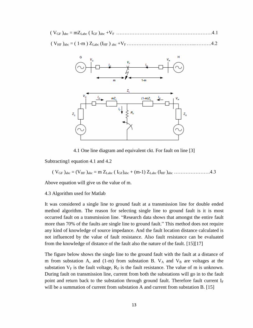
( VGF )abc = mZLabc ( IGF )abc +VF ………………………………………………….4.1
( VHF )abc = ( 1-m ) ZLabc (IHF ) abc +VF …………………………………...……….4.2
4.1 One line diagram and equivalent ckt. For fault on line [3]
Subtracting1 equation 4.1 and 4.2
( VGF )abc = (VHF )abc = m ZLabc ( IGF)abc + (m-1) ZLabc (IHF )abc ………………….4.3
Above equation will give us the value of m.
4.3 Algorithm used for Matlab
It was considered a single line to ground fault at a transmission line for double ended
method algorithm. The reason for selecting single line to ground fault is it is most
occurred fault on a transmission line. “Research data shows that amongst the entire fault
more than 70% of the faults are single line to ground fault.” This method does not require
any kind of knowledge of source impedance. And the fault location distance calculated is
not influenced by the value of fault resistance. Also fault resistance can be evaluated
from the knowledge of distance of the fault also the nature of the fault. [15][17]
The figure below shows the single line to the ground fault with the fault at a distance of
m from substation A, and (1-m) from substation B. VA and VB are voltages at the
substation VF is the fault voltage, RF is the fault resistance. The value of m is unknown.
During fault on transmission line, current from both the substations will go in to the fault
point and return back to the substation through ground fault. Therefore fault current IF
will be a summation of current from substation A and current from substation B. [15]
14
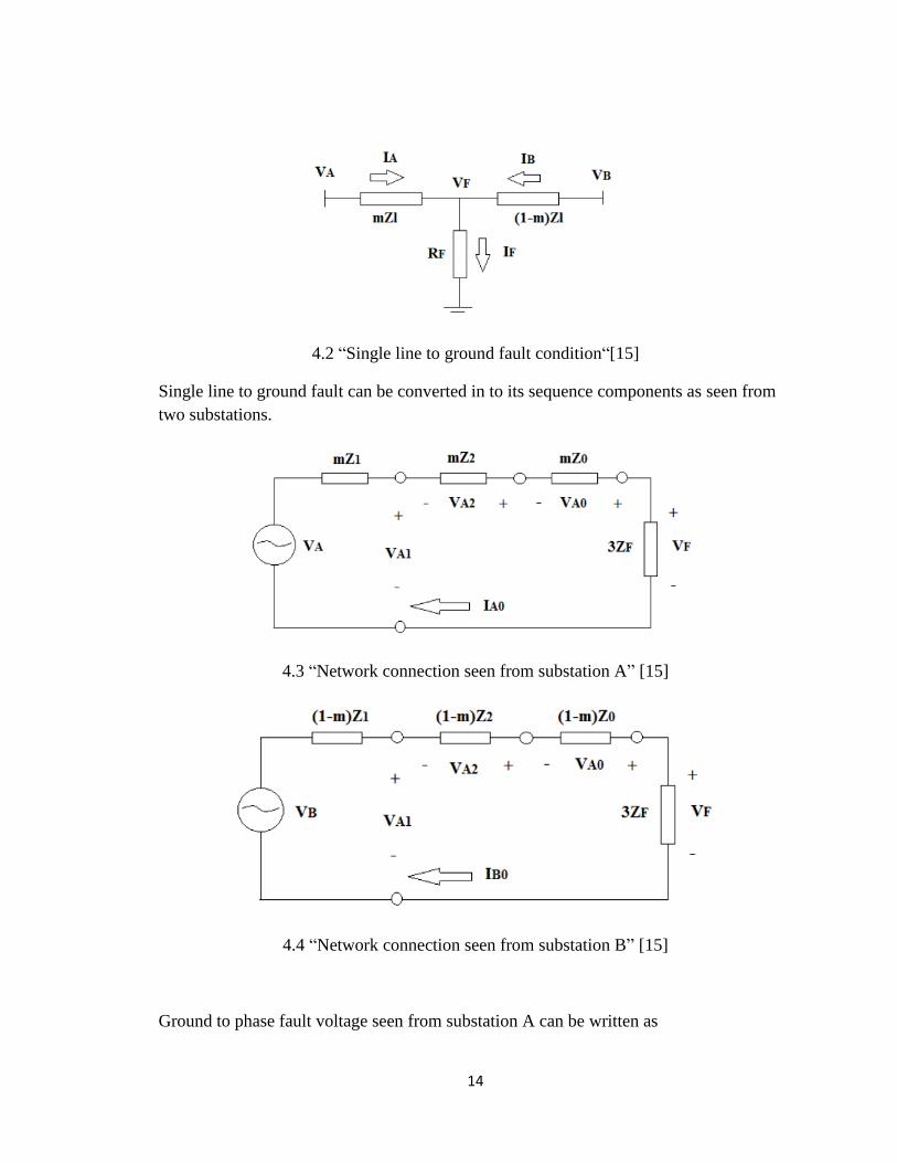
4.2 “Single line to ground fault condition“[15]
Single line to ground fault can be converted in to its sequence components as seen from
two substations.
4.3 “Network connection seen from substation A” [15]
4.4 “Network connection seen from substation B” [15]
Ground to phase fault voltage seen from substation A can be written as

15
VF = VA – m (Z1 + Z2 + Z0 ) ……………………………….………..4.4
Similarly Ground to phase fault voltage seen from substation B can be written as
VF = VB – (1-m) (Z1 + Z2 + Z0 )…………………………….……….4.5
Equating 4.4 and 4.5
VA – m (Z1 + Z2 + Z0 ) = VB – (1-m) (Z1 + Z2 + Z0 ) ……………..4.6
Also for both the substation phase current zero sequence current components are equal
IA0 = IA / 3 …………………………………………….…………….4.7
IB0 = IB / 3 …………………………………………..………………4.8
Therefore from above equations, we can calculate the value of m as
m = …………………………………………4.9

16
5. Fault Location on distribution Lines
5.1 Introduction
“The problem of fault location has been studied deeply for transmission lines and is
revealing special attention mainly because of power quality regulations. Various
methods have been discussed for the location of fault on distribution lines. But somehow
these methods are not easily applicable to distribution systems because these use
measures from two terminal lines, the non-homogeneity, presence of lateral and load taps
on distribution lines.”[13]
Fault location techniques are classified in following different categories:
Classical approach that measures fundamental voltage and currents.
Traveling wave theory technique.
Topological method approach.
Knowledge based approach.
5.2 Different Approach
In this chapter we will review the classical approach and knowledge based approach and
also a hybrid approach based on both.
1. Ratan Das Method
This method measures the voltages and the current at a line terminal prior to the fault and
during the fault.[12] This method consists of 6 steps for the fault location:
An estimate of the probable fault location is made from the line parameters and
phasors of sequence voltage and currents.
All laterals in between the fault location and the initial node are ignored and all
the load connected to lateral is assumed to be connected to the node where the
lateral is connected.
Load effects (static response type models) are considered by compensation of
their currents up to the node just before the faulty node and for a load at remote
end.
All the loads beyond faulty node are considered into a single load at the remote
end node and hence the fault sequence voltages and currents are calculated at
node F.
Using the voltage current relationships, the location of the fault is estimated.

17
If the line has laterals, we may get multiple estimates for the fault and hence we
have to convert it to a single estimate. For this purpose, much soft wares are
available which convert it down to a single estimate.
2. Mourari Saha Method
“The approach proposed by Saha [13] measures the fundamental frequency voltages and
currents measured at a line terminal prior to a fault and during a fault. It implies the
estimation of distance to fault on a radial MV system which includes many intermediate
load taps by using topology principle.” The calculation of fault location is done by two
steps:
From the calculated data of voltages and currents we measure the fault loop
impedance.
By considering the faults at each successive section, the impedance along the
feeder is calculated.
Thereby comparing the measured impedance with the feeder impedance, an estimation of
fault location could be obtained, and hence the distance to the fault can be estimated.
The following formula is proposed to estimate a phase-phase fault loop impedance:
ZK = ………………….5.2.2.1
Where Vpp – “phase to phase fault loop voltage”
Ipp- “phase to phase fault loop current”
Zpre – “impedance in pre fault conditions”
Kzk – “relation between the power in faulty lines and power in all the lines”
In phase to ground fault, the fault loop impedance is obtained as:
Zk = …………………………5.2.2.2
Where Zg = Vph/ (Iph+KknIkn)……………………5.2.2.3
V0= (VA + VB+ VC )/3……………………….5.2.2.4
3. The method of superimposed components
To estimate fault in radial distribution lines with several load taps we used the method of
superimposed components. For overhead distribution systems [14] this method does

18
single ended fault location. The difference between pre fault and post fault voltage, i.e.
known as superimposed voltage is calculated. We inject this voltage at an assumed fault
point to find current in other phases. The injected currents attain a zero value at the actual
fault point.
The relation between the voltages at assumed faults to measured voltages and currents is
given by:
= β + ……………..5.2.3.1
Where β is the assumed fault location
Zs and Zm are self and mutual line impedance
Vs and Is the measured voltages and current.
The superimposed voltages are thus obtained as
[V’fa,b,c (β)] =[Vfa,b,c (β)]-[ Vfa,b,c (ss) (β)]…………….5.2.3.2
And the superimposed currents and voltages at measuring point are given by
[V’Sa,b,c ] =[ VSa,b,c ]-[ VSa,b,c (ss) ]….5.2.3.3
[I’Sa,b,c ] = [ ISa,b,c ]-[ Isa,b,c (ss) ]........5.2.3.4
“For a feeder with multiple taps the computational process is complex however the same
principal can be applied.
To represent a load we need to:
Measure primary impedance of the transformer assuming a power facto between
0.8 to 0.95.
Type of tap
Single phase or three phase”
For the first case impedance is given by following equation:
ZL = cos-1
φ ….5.2.3.5
For the second case:
ZL =3 cos-1
φ …..5.2.3.6
Where M is the nominal transformer rating
Vl is the voltage at the load point.
Using the above impedances we can set up a load matrix. “Impedance is supposed to be
considered, when a line section is terminated by a primary substation.”
Load level is then calculated to study the variation of the load with time of day to
determine the load impedance. Load level is the ratio between the active power fed to
feeder at the measuring point and maximum total load.

19
PSS = sqrt 3 VlssILSS cos φ……..5.2.3.7
Plmax = (M1+ M2 + M……Mn) cos φ …..5.2.3.8
Where M is the nominal transformer ratio
N is the number of load taps
Therefore
L level = …….5.2.3.9
Hence the impedance of the single phase load tap is given as
ZL = cos-1
φ …….5.2.3.10
Therefore by using this method we get a high accuracy for the majority of systems and
fault conditions.
4. The hybrid approach of algorithmic based method and knowledge based
Several other approaches are used in the fault location which implements the use of
current/voltage sensors, fault recorders and a good system modal. But this proposal is
based on a voltage sag and their currents and hence extracting significant information
from them. The information provided is based on the disturbance.
This approach aims at deriving information from the recorded signal of voltage and
current during pre-fault conditions and during the fault. Most of the algorithmic methods
are based on the stable state information from the fault whereas some other techniques
such as neutral nets use vector machines etc to measure the transient information.
Therefore as the output of this knowledge based approaches, it describes how to set the
algorithmic methods.
“To locate the fault, it is possible to use a well-known algorithmic method using state
stable data from the fault registers. Using the result derived from the application of
algorithmic method different set of possible fault locations is obtained. At last an
intersection of the two possible sets of fault obtained from the two different methods is
used to have the most appropriate fault location.”[14]
5.3 Conclusion
Location of fault using the available voltage and current implies saving of great amount
of money to the distribution electrical utilities. These results are meaningful in both
network planning and network operation. In planning it aims at the design and assessment
of sensitive equipment and improving the designs of protection system.

20
6. Fault Location Matlab Simulation
A transmission line was modeled using Matlab Simulink. The analysis of single line to
ground fault location was performed. I used the SimPowerSystem toolbox to perform the
simulation.
Table below represents the parameters of line used for the analysis
Parameters of Lines Value
Length Varying
Normal Frequency 60 Hz
Voltage Phase to phase 132 KV
Resistance Positive sequence .045531917 ohms/Km
Resistance Zero Sequence .0151489359 ohms/Km
Inductance Positive Sequence .000617657 Henry/Km
Inductance Zero Sequence .001533983 Henry/Km
Table 6.1 Parameters of the line used for analysis
Following diagrams shows the transmission line model. It is modeled using distributed
parameter line.
VG
IG
LOAD
m
Fault
G F
Fig 6.1 Single line diagram for single ended method fault location

21
6.2 Transmission line Schematic using Matlab/Simulink for single ended method
6.3 Transmission line model with fault location calculation for single ended method

22
IA
m
Fault
A B
VAVB
IB
Fig 6.4 Single line diagram for double ended fault location
6.5 Transmission line Schematic using Matlab/Simulink for duble ended method
6.6 Transmission line model with fault location calculation for double ended method
23
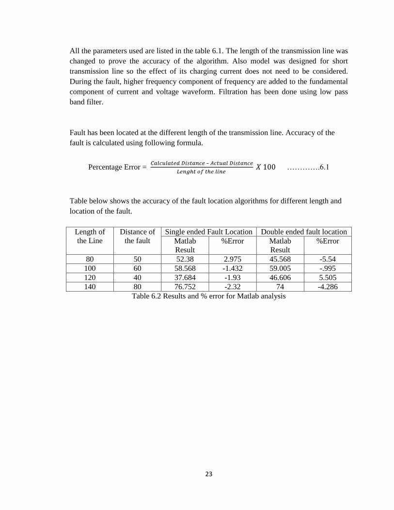
All the parameters used are listed in the table 6.1. The length of the transmission line was
changed to prove the accuracy of the algorithm. Also model was designed for short
transmission line so the effect of its charging current does not need to be considered.
During the fault, higher frequency component of frequency are added to the fundamental
component of current and voltage waveform. Filtration has been done using low pass
band filter.
Fault has been located at the different length of the transmission line. Accuracy of the
fault is calculated using following formula.
Percentage Error = –
………….6.1
Table below shows the accuracy of the fault location algorithms for different length and
location of the fault.
Length of
the Line
Distance of
the fault
Single ended Fault Location Double ended fault location
Matlab
Result
%Error Matlab
Result
%Error
80 50 52.38 2.975 45.568 -5.54
100 60 58.568 -1.432 59.005 -.995
120 40 37.684 -1.93 46.606 5.505
140 80 76.752 -2.32 74 -4.286
Table 6.2 Results and % error for Matlab analysis

24
7. Conclusion
If power system is homogeneous, and mutual coupling between transmission line
is weak, single ended method can be used with large accuracy.
Traveling wave method is much reliable when time synchronization and other
needful equipment is available.
Double ended fault location algorithm can highly improve the accuracy of fault
location. Algorithm used in the project can be used best where fault disturbance
recorders or microprocessor relays are available because fault location
calculations does not get affected by fault resistance, in-feed effect, different
source impedance value.
25
References
[1] “Fault location on power network” M. M. Saha, E. Rosolowski, J. Izykowski.
Springer publication 2010.
[2] “Review of fault location techniques for transmission and sub transmission lines” Das
R., Novosel D. Proc of 54th Annual Georgia Tech Protective Relaying Conference 2000
[3] “IEEE guide for determining fault location on AC transmission line and distribution
lines.” IEEE std C37.144 2004
[4] “Fault location on power transmission lines” Izykowski J. Techniczeskaja
Elektrodinamika, 2002
[5] “Fault Location” Kezunovic M
[6] “A review of impedance based fault locating experience” Schweitzer EO III. SEL
1990
[7] “Traveling Wave Fault Location in Power Transmission Systems “Hewlett-Packard
company 1997.
[8] “Development of a new fault locator using the one-terminal voltage and current data”
Takagi al. Power Apparatus and Systems, IEEE Transactions 2892 - 2898, Aug 1982
[9] “On line digital fault locator for overhead transmission line,” Sant and Y. Paithankar
IEEE transaction 8398 P, 1979.
[10] “A technique for estimating transmission line fault locations from digital impedance
relay measurements,” M. Sachdev and R. Agarwal, IEEE Transactions on Power
Delivery, Vol. 3, No. 1, January 1988
[11] “An overview to fault location methods in distribution system based on single end
measures of voltage and current.” J.Mora, Manel Castro.
[12] “A fault location for radial subs transmission and distribution lines.” Das R, Sachdev
M, Sidhu T. Engineering Society Summer Meeting, 2000. IEEE, Volume: 1
[13] “Fault location method for MV cable network.” Saha M , Provoost F. Developments
in Power System Protection, 2001, Seventh International Conference on (IEE)
[14] “New concept in fault location for overhead distribution systems using
superimposed components.” Aggarwal R.K , Aslan Y. Generation, Transmission and
Distribution, IEE Proceedings Pages 309-316, 1997.

26
[15] “Effective Two-Terminal Single Line to ground fault location algorithm” M.H. Idris,
M.W.Mustafa, Y. Yatim, Power Engineering and Optimization Conference (PEDCO)
Melaka, Malaysia, 2012 Ieee International Pages 246-251
[16] “The Application of Fault Signature Analysis in Tenaga Nasional Berhad Malaysia”
A. M. Zin, S. P. A. Karim, Power Delivery, IEEE Transactions Pages 2047-2056, 2007
[17] “Evaluation and Development of Transmission Line Fault-Locating Techniques
Which Use Sinusoidal Steady-State” E.Schwetzer SEL 1982
[18] M. “A Technique for Estimating Transmission Line Fault Locations From Digital
Impedance Relay Measurements” Sachdev and R. Agarwal. IEEE Transactions on Power
Delivery, Vol. 3, No. 1, January 1988
[19] “Fault location on two-terminal transmission lines based on voltages” I. Zamora, J.
F. Miambres, A. J. Mazn, R. Alvarez-Isasi and J. Lazaro. IEE, 1996 IEE Proceedings
online no. 199601 12.