Fault Detection for Mobile Robots based on Integrated Sensor...
118
Fault Detection for Mobile Robots based on Integrated Sensor Systems Relat ´ orio submetido ` a Universidade Federal de Santa Catarina como requisito para a aprovac ¸˜ ao da disciplina: DAS 5511: Projeto de Final de Curso Andr ´ e C. Bittencourt Florian ´ opolis, abril de 2009
Transcript of Fault Detection for Mobile Robots based on Integrated Sensor...

Fault Detection for Mobile Robotsbased on Integrated Sensor Systems
Relatorio submetido a Universidade Federal de Santa Catarina
como requisito para a aprovacao da disciplina:
DAS 5511: Projeto de Final de Curso
Andre C. Bittencourt
Florianopolis, abril de 2009

Fault Detection for Mobile Robots based on IntegratedSensor Systems
Andre C. Bittencourt
Orientador:
Prof. Bo Wahlberg
Este relatorio foi julgado no contexto da disciplinaDAS 5511: Projeto de Fim de Curso
e aprovado na sua forma final peloCurso de Engenharia de Controle e Automacao Industrial
ii

Banca Examinadora:
Prof. Bo WahlbergOrientador Instituto
Prof. Alexandre TrofinoOrientador do Curso
Prof. Augusto Humberto BruciapagliaResponsavel pela disciplina
Prof. Ubirajara Franco Moreno, Avaliador
Daniel Fernandes de Souza, Debatedor
Caio Merlini Giuliani, Debatedor

Abstract
Most fault detection algorithms are based on residuals, i.e. the difference be-
tween a measured signal and the corresponding model based prediction. However, in
many more advanced sensors the raw measurements are internally processed before
refined information is provided to the user.
The contribution of this thesis is a study of the fault detection problem when only
the state estimate from an observer/Kalmanfilter is available and not the measured
residual/innovation. The idea is to look at an extended state space model where the
true states and the observer states are combined. This extended model is then used
to generate residuals viewing the observer outputs as measurements. Results for fault
observability of such extended models are given. The approach is rather straightfor-
ward in case the internal structure of the observer is exactly known. For the Kalman
filter this corresponds to knowing the observer gain. If this is not the case certain model
approximations can be done to generate a simplified model to be used for standard fault
detection.
Our motivating application has been mobile robots where the so-called pose, the
position and orientation of the robot, is an important quantity that has to be estimated.
The pose can be measured indirectly from several different sensor systems such as
odometry, computer vision, sonar and laser. The output from these so-called pose
providers are often state estimates together with, in best cases, an error covariance
matrix estimate from which it might be difficult or even impossible to access the raw
sensor data since the sensor and state estimator/observer are often integrated and
encapsulated. In this thesis we discuss some of the main pose estimators in mobile
robots and validate a fault detector filter through experiments using the our proposed
framework.
iv

Acknowledgments
This thesis was held at the Royal Institute of Technology (KTH) Automatic Con-
trol Department, Sweden. I would like to thank all my colleagues, students and em-
ployees, at KTH for the nice moments we shared during my stay in Stockholm pro-
portionating a nice work atmosphere. Special thanks for my supervisor, Bo Wahlberg,
for providing me the opportunity to join the project who, together with Patric Jensfelt
at the Centre of Autonomous Systems, have shared their knowledge/expertizing and
provided an always nice but challenging environment.
Finally, this work would have never come true if it was not for the help and sup-
port given from good friends and specially from my family. Thank you very much for
everything.
i

Resumo Estendido
Grande parte dos algoritmos de deteccao de falhas sao baseados em resıduos,
i.e. a diferenca entre um sinal medido e uma correspondente predicao baseada em
modelo. No entanto, em muitos sensores mais avancados, as medidas puras sao
internamente processadas antes que informacao refinada seja repassada ao usuario.
A primeira contribuicao deste trabalho e o estudo do problema de deteccao de
falhas quando somente estimacao de estados obtidas por um observador ou filtro de
Kalman estao disponıveis, mas nao seus resıduos/inovacoes. A ideia e olhar para
um modelo de espaco de estados extendido onde os estados reais e os estados do
observador estao combinados. Este modelo extendido pode entao ser utilizado para
gerar resıduos utilizando as saıdas do sensor integrado e suas entradas como valores
medidos. Resultados para observabilidade de falhas utilizando tal modelo extendido
sao dadas. A abordagem e consideravelmente simples em caso a estrutura interna do
sensor e exatamente conhecida. Para o filtro de Kalman, correspondendo a saber o
ganho do observer usado no sensor. Se este nao e o caso, simplificacoes podem ser
realizadas para gerar um modelo simplificado a ser usado na deteccao de falhas.
Uma questao importante e discutir os ganhos utilizados usando-se tal mod-
elo, indicacoes para o problema sao apresentados atraves da analise das funcoes de
transferencia falha-resıduo, para os diversos casos. Especialmente interessante e a
comparacao entre as abordagens em que se utiliza do conhecimento da estrutura in-
terna do sensor (ganho do observador, por exemplo) em contrapartida ao que se faz
simplificacoes quanto ao sensor.
Nossa aplicacao motivadora tem sido robotica movel onde a conhecida pose
do robo, sua posicao e orientacao, e uma importante grandeza a ser estimada. A
pose pode ser medida indiretamente por diferentes sensores como odometria, visao
computacional, sonar e laser. A saıda destes “provedores de pose” sao geralmente es-
tados estimados, juntamente com, nos melhores dos casos, uma estimativa da matriz
de covariancia de erros, pode ser difıcil ou ate mesmo impossıvel de se ter acesso as
grandezas diretamente medidas por estes sensores, uma vez que os mesmos estao
geralmente integrados e encapsulados com observadores/estimadores de estados.
ii

Neste trabalho, nos tambem discutimos alguns dos provedores de pose em robos
moveis e apresentamos e validamos uma framework para deteccao e atuenacao de
falhas de localizacao em alguns cenarios relevantes.
Um sistema de monitoramento de condicao supervisiona um sistema dinamico
com o objetivo de:
• Detectar falhas: o sistema reconhece que uma falha ocorreu.
• Isolar falhas: o sistema reconhece onde e quando uma falha ocorreu (alguns
sistemas incluem as funcoes de reconhecer o tipo de falha, o tamanho ou a
causa da falha).
• Atenuar falhas: o sistema toma medidas necessarias para contra atuar os efeitos
das falhas.
Nossa framework define cada uma dessas funcoes. Para tal, primeiramente, apre-
sentamos dois provedores de localizacao utilizados comumente em robotica movel,
odometria e sobreposicao de scans laser. Suas princıpias caracterısticas e alguns al-
goritmos sao motivos de estudo. Os mesmos sao utilizados em um robo movel para
na nossa framework que inclue as tarefas de deteccao de falhas, estimacao do seu
tempo de ocorrencia, estimacao do seu tamanho e atenuacao sobre as estimacoes de
pose providas pela odometria.
As contribuicoes mais relevantes deste trabalho sao:
• As condicoes de detectabilidade de falhas para tais sensores integrados atraves
da analise de observabilidade do sistema augmentando as falhas nas matrizes
de dinamica apresentadas no Capıtulo 4.
• A analise da sensibilidade das funcoes de transferencia falha-resıduo para as
solucoes propostas presente no Capıtulo 4.
• A framework utilizada para detectar, isolar e atenuar falhas na localizacao de
robos moveis, objeto de estudo do Capıtulo 6.
• O paper aceito para o 7th IFAC Symposium on Fault Detection, Supervision and
Safety of Technical Processes incluso no Anexo A.
iii

Summary
1 Introduction 1
1.1 Residual Based Fault Detection using Observer Data Only . . . . . . . . 3
1.2 Outline . . . . . . . . . . . . . . . . . . . . . . . . . . . . . . . . . . . . . 4
1.3 Contributions . . . . . . . . . . . . . . . . . . . . . . . . . . . . . . . . . 5
I Fault detection 6
2 Fault detection review 7
2.1 Fault Detection and Isolation Overview . . . . . . . . . . . . . . . . . . . 7
2.1.1 Fault Detection and Isolation Methods . . . . . . . . . . . . . . . 8
2.2 Model-based FDI methods . . . . . . . . . . . . . . . . . . . . . . . . . 9
2.2.1 Residual generation methods - parameter estimation . . . . . . . 11
2.2.2 Residual generation methods - state estimation (observers) . . . 14
2.3 Change (fault) detection methods . . . . . . . . . . . . . . . . . . . . . . 16
2.4 Concluding Remarks . . . . . . . . . . . . . . . . . . . . . . . . . . . . . 18
3 State observers 20
3.1 State observers . . . . . . . . . . . . . . . . . . . . . . . . . . . . . . . . 20
3.2 State estimation - The Kalman filter . . . . . . . . . . . . . . . . . . . . . 21
3.2.1 The filter algorithm . . . . . . . . . . . . . . . . . . . . . . . . . . 22
3.2.2 The extended Kalman filter . . . . . . . . . . . . . . . . . . . . . 23
3.3 Observability conditions . . . . . . . . . . . . . . . . . . . . . . . . . . . 24
iv

3.3.1 The observability matrix . . . . . . . . . . . . . . . . . . . . . . . 24
3.3.2 The Popov-Belevitch-Hautus criteria . . . . . . . . . . . . . . . . 25
3.4 Concluding remarks . . . . . . . . . . . . . . . . . . . . . . . . . . . . . 26
4 Observer-based fault detection 27
4.1 Observer-based residual generation - classical approach . . . . . . . . 27
4.1.1 Fault observability . . . . . . . . . . . . . . . . . . . . . . . . . . 28
4.1.2 Residual analysis . . . . . . . . . . . . . . . . . . . . . . . . . . . 29
4.1.2.1 Fault sensitivity . . . . . . . . . . . . . . . . . . . . . . . 30
For additive input sensor faults . . . . . . . . . . . . . . . 30
For additive process faults . . . . . . . . . . . . . . . . . . 32
For additive output sensor faults . . . . . . . . . . . . . . 33
4.1.2.2 Some remarks . . . . . . . . . . . . . . . . . . . . . . . 34
4.2 Observer-based residual generation through integrated sensors . . . . 34
4.2.1 Fault observability . . . . . . . . . . . . . . . . . . . . . . . . . . 35
For s 6= 1 . . . . . . . . . . . . . . . . . . . . . . . . . . . 38
For s = 1, . . . . . . . . . . . . . . . . . . . . . . . . . . . 40
4.2.2 Residual analysis . . . . . . . . . . . . . . . . . . . . . . . . . . . 41
4.2.2.1 Fault sensitivity . . . . . . . . . . . . . . . . . . . . . . . 43
For additive input sensor faults . . . . . . . . . . . . . . . 43
For additive process faults . . . . . . . . . . . . . . . . . . 44
For additive output sensor faults . . . . . . . . . . . . . . 45
4.2.2.2 Some remarks . . . . . . . . . . . . . . . . . . . . . . . 45
4.2.3 Residual generation - Unknown sensor structure . . . . . . . . . 46
4.2.3.1 Residual analysis . . . . . . . . . . . . . . . . . . . . . 47
4.2.3.2 Fault sensitivity . . . . . . . . . . . . . . . . . . . . . . . 48
For additive input sensor faults . . . . . . . . . . . . . . . 48
v

For additive process faults . . . . . . . . . . . . . . . . . . 49
For additive output sensor faults . . . . . . . . . . . . . . 49
4.2.3.3 Some remarks . . . . . . . . . . . . . . . . . . . . . . . 50
4.3 Concluding remarks . . . . . . . . . . . . . . . . . . . . . . . . . . . . . 50
Noise and uncertainties . . . . . . . . . . . . . . . . . . . 51
Optimal residual and the observer design . . . . . . . . . 51
Kalman filtering . . . . . . . . . . . . . . . . . . . . . . . . 52
II Application example 53
5 Wheeled Mobile robots 54
5.1 Robot modeling . . . . . . . . . . . . . . . . . . . . . . . . . . . . . . . . 55
5.2 Pose providers . . . . . . . . . . . . . . . . . . . . . . . . . . . . . . . . 56
5.3 Odometry . . . . . . . . . . . . . . . . . . . . . . . . . . . . . . . . . . . 57
5.3.1 Error sources . . . . . . . . . . . . . . . . . . . . . . . . . . . . . 57
5.3.2 Error modeling . . . . . . . . . . . . . . . . . . . . . . . . . . . . 59
5.4 Laser scan matching . . . . . . . . . . . . . . . . . . . . . . . . . . . . . 60
5.4.1 Iterative Closest Point - ICP . . . . . . . . . . . . . . . . . . . . . 62
5.4.2 Matching in the Hough domain - HSM . . . . . . . . . . . . . . . 65
5.4.2.1 Rotation estimation through spectra correlation . . . . . 67
5.4.2.2 Complexity . . . . . . . . . . . . . . . . . . . . . . . . . 68
5.5 Concluding remarks . . . . . . . . . . . . . . . . . . . . . . . . . . . . . 69
6 Fault detection and recovery 71
6.1 Change detection . . . . . . . . . . . . . . . . . . . . . . . . . . . . . . . 72
6.1.1 Residual generation . . . . . . . . . . . . . . . . . . . . . . . . . 73
6.1.1.1 ε0 - difference between poses . . . . . . . . . . . . . . 74
vi

6.1.1.2 ε - observer with unknown sensor structure . . . . . . . 74
6.1.1.3 ε - augmented observer . . . . . . . . . . . . . . . . . . 76
6.1.2 Distance measure . . . . . . . . . . . . . . . . . . . . . . . . . . 78
6.1.3 Stopping rule . . . . . . . . . . . . . . . . . . . . . . . . . . . . . 78
6.1.4 Case studies . . . . . . . . . . . . . . . . . . . . . . . . . . . . . 79
6.1.4.1 Case 1: Normal case . . . . . . . . . . . . . . . . . . . 79
6.1.4.2 Case 2: Hard fault . . . . . . . . . . . . . . . . . . . . . 81
6.1.4.3 Case 3: Slippage fault . . . . . . . . . . . . . . . . . . . 81
6.1.4.4 Conclusions . . . . . . . . . . . . . . . . . . . . . . . . 83
6.2 Fault isolation and recovery . . . . . . . . . . . . . . . . . . . . . . . . . 84
6.2.1 Fault isolation . . . . . . . . . . . . . . . . . . . . . . . . . . . . . 85
6.2.2 Recovery . . . . . . . . . . . . . . . . . . . . . . . . . . . . . . . 89
6.2.3 Case studies . . . . . . . . . . . . . . . . . . . . . . . . . . . . . 89
6.3 Concluding remarks . . . . . . . . . . . . . . . . . . . . . . . . . . . . . 91
7 Conclusions 93
7.1 Summary . . . . . . . . . . . . . . . . . . . . . . . . . . . . . . . . . . . 93
7.2 Future work . . . . . . . . . . . . . . . . . . . . . . . . . . . . . . . . . . 93
Bibliography 95
Annex A -- Paper I 101
vii

1 Introduction
Sensors and observers/estimators are often closely integrated in intelligent sen-
sor systems. This situation is common in distributed sensor processing applications. It
may be very difficult or even impossible to access the raw sensor data since the sensor
and state estimator/observer are often integrated and encapsulated.
An important application of sensor based systems is model based fault detec-
tion, where the sensor information is used to detect abnormal behavior. The typical
approach is to study the size of certain residuals (differences between a direct mea-
sured output y(k) and a redundant model-based prediction of the same, y(k)), that
should be small in case of no fault, and large in case of faults. Most of these methods
rely on the direct sensor measurements. The problem when only state estimates are
available, as depicted in Figure 1.1, is less studied. In [1] the fault detection using such
(a) Raw measurements available. (b) Only an integrated sensor output available.
Figure 1.1: Residual generation problem arising when raw measures are not available.
sensors in mobile robotics is discussed from mainly an experimental point of view. The
primary objective of this thesis is to investigate the theoretical foundation of observer
data only fault detection, where it is not possible to directly access the raw sensor data.
Our motivating application has been mobile robots, where the localization task
(estimating the robot positioning) plays an important role for increasing the general per-
formance and reliability of the robot. The methods available today commonly provide
an estimate which is the result of some internal computations from raw measurements,
including in this category relative localization methods, .i.e dead-reckoning, and even
global positioning systems, i.e. triangularization/trilateron. It may be difficult or or even
impossible to access the raw measured data used in such methods and one should
deal with the fault detection problem only with the estimates provided.
1
2
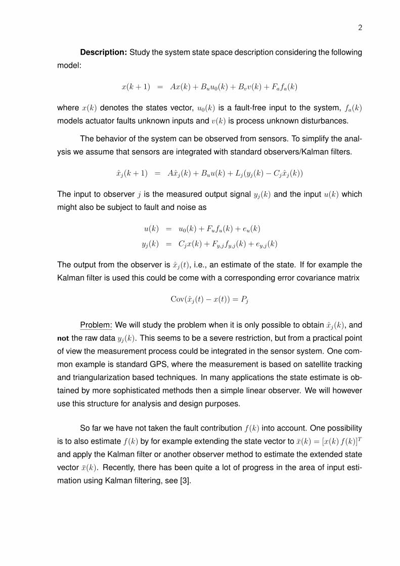
Description: Study the system state space description considering the following
model:
x(k + 1) = Ax(k) +Buu0(k) +Bvv(k) + Fafa(k)
where x(k) denotes the states vector, u0(k) is a fault-free input to the system, fa(k)
models actuator faults unknown inputs and v(k) is process unknown disturbances.
The behavior of the system can be observed from sensors. To simplify the anal-
ysis we assume that sensors are integrated with standard observers/Kalman filters.
xj(k + 1) = Axj(k) +Buu(k) + Lj(yj(k)− Cjxj(k))
The input to observer j is the measured output signal yj(k) and the input u(k) which
might also be subject to fault and noise as
u(k) = u0(k) + Fufu(k) + eu(k)
yj(k) = Cjx(k) + Fy,jfy,j(k) + ey,j(k)
The output from the observer is xj(t), i.e., an estimate of the state. If for example the
Kalman filter is used this could be come with a corresponding error covariance matrix
Cov(xj(t)− x(t)) = Pj
Problem: We will study the problem when it is only possible to obtain xj(k), and
not the raw data yj(k). This seems to be a severe restriction, but from a practical point
of view the measurement process could be integrated in the sensor system. One com-
mon example is standard GPS, where the measurement is based on satellite tracking
and triangularization based techniques. In many applications the state estimate is ob-
tained by more sophisticated methods then a simple linear observer. We will however
use this structure for analysis and design purposes.
So far we have not taken the fault contribution f(k) into account. One possibility
is to also estimate f(k) by for example extending the state vector to x(k) = [x(k) f(k)]T
and apply the Kalman filter or another observer method to estimate the extended state
vector x(k). Recently, there has been quite a lot of progress in the area of input esti-
mation using Kalman filtering, see [3].

3
1.1: Residual Based Fault Detection using Observer DataOnly
Residual based techniques are all based on comparing the predicted output
y(k), based on a model, with the observed output y(k). In case of a systematic differ-
ence we will alarm. If only x(k) is available the first two ideas for fault detection ideas
would be:
• Try to reconstruct y(k) using a model of the observer, e.g.
Ljyj(k) = xj(k + 1)− (A− LjCj)xj(k)−Buu(k)
Here we need a very accurate model and the internal structure of the observer,
e.g. the gain L, otherwise the estimations will be easily biased. In many practical
cases this would be difficult. Notice also that if Lj is not full rank, it allows for
multiple solutions.
• Assume that there are at least two observers providing x1(k) and x2(k). Define
the residual vector
ε(t) = x1(k)− x2(k)
which should be sensible to fault that affects the two observers in different ways,
e.g. sensor faults. This approach does not, however, make direct use of the model
of the system.
We will start by analyzing the case with only one observer.
Idea: View x(k) as the output from the extended system
x(k + 1) = Ax(k) +Buu(k) + Fafa(k)
x(k + 1) = Ax(k) +Buu(k) + L(y(k)− Cx(t))
y(k) = C∗x(k), where y(k) = Cx(k) + Fyfy(k)
where C∗ depicts which estimates are available. By using the extended state x(k) =
[xT (k) xT (k)]T and the corresponding state space matrices we can interpret this a
standard fault detection problem, which could be approached by a parity space method
or a Kalman filter based method. The problem when we have m different observers
can be approached by augmenting the state space x(k) with all observer states xj(k),
j = 1, . . .m.

4
There are some basic questions that need to be addressed with such framework
which are studied in this thesis:
• Are the faults detectable using this model?
• What to do if the sensor gain L is unknown?
• How to compare/validate the performance of different methods?
1.2: Outline
This thesis is divided in two parts. Part I approaches the problem in a more
theoretical manner, analyzing some of its properties and proposed solutions. Part II
presents a practical example in detection of localization faults in mobile robots. Starting
with Part I, it follows as:
Chapter 2 presents a review on fault detection with a brief introduction to the
main different methods and paradigms.
Chapter 3 is an introduction to state observers and some relevant properties for
this work.
Chapter 4 presents some theoretical analysis on observer-based fault detection
for both when one has access to y(k) or only y(k), and addresses the questions on
fault observability, fault sensitivity and unknown sensor structure (for the latter case).
Chapter 5 starts Part II with our application example. It describes the platform
used, wheeled mobile robots. It includes a discussion on modeling and localization
methods with more emphases on odometry and laser scan matching.
Chapter 6 presents an approach for fault detection in wheeled mobile robots.
Different methods are used which are compared and analyzed.
Finally, Chapter 7 concludes this work and leave comments on remaining chal-
lenges.
Moreover, in Appendix A, we include the conference paper to be presented in
the 7th SAFEPROCESS.

5
1.3: Contributions
The main contributions of this thesis are:
• The fault observability conditions for integrated sensors presented in Chapter 4.
• The analysis on residuals fault sensitivity for the different methods and compari-
son presented in Chapter 4.
• The fault detection framework for localization faults in mobile robots presented in
Chapter 6.
• The conference paper in Appendix A.

Part I
Fault detection
6

2 Fault detection review
This Chapter presents a review on the main aspects of fault detection and isola-
tion (FDI) methods with focus on the application to localization fault detection in mobile
robots.
2.1: Fault Detection and Isolation Overview
This Section was based on [5, 12, 17] and provides the reader with a brief
overview of FDI (Fault Detection and Isolation) methods. Basically, the purpose of
FDI is to monitor dynamic systems and should be able to perform the following tasks:
• Fault detection: FDI recognizes that a fail has occurred.
• Fault isolation: FDI recognizes where and when a fail has occurred (some FDI
extend this concept to include the type, size or cause of the fail).
To choose the algorithm of the FDI it is important to know which kind of fault is
present in the system. Basically the fault types can be classified by its time behavior
and effects on the system.
The first category of fault can be summarized as:
• Abrupt: faults that affect the system in a stepwise manner. Ex: A wrong calibra-
tion of a sensor causing an offset like error.
• Incipient: faults that occur gradually with time (drift-like). Ex: increase of friction
inside a gearbox due to wear.
• Intermittent: faults that affect the system during certain time intervals, with inter-
rupts. Ex: undesired air bubbles in a gas pipeline.
7

CHAPTER 2. FAULT DETECTION REVIEW 8
The manner a fault affects the system’s behavior can be categorized as:
• Additive: faults that are effectively added to the system’s input or output. Ex:
sensor faults.
• Multiplicative: faults that changes the parameters of the system. Ex: resistance
changes in an electric motor caused by an overheat.
• Structural: faults that introduces new governing terms to the describing equations
of the system. Ex: a change on the dynamic behavior of an aircraft caused by a
loss of power in the engines.
Figure 2.1 illustrates additive faults in the input signal (fu) and output signal (fy)
as well as a multiplicative faults (fpar) of a system.
Figure 2.1: Additive and Multiplicative faults.
Remark 1 Localization faults are generally associated with a malfunction of a localiza-
tion provider and affects an output of the system. Therefore, it can be classified as an
additive fault that may occur abruptly or in an incipient manner.
Fault detection methods can either run on-line (concomitantly to the normal op-
eration of the system) or off-line (achieved for example with special experiments for
diagnosis). The methods and complexity for each of these category vary considerably,
with on-line methods remaining the biggest challenge.
2.1.1: Fault Detection and Isolation Methods
FDI methods can rely or not on a model of the system. Three convenient cate-
gories for model-free methods are:
• Hardware redundancy: these systems rely on extra hardware which are specially
used to detect faults.

CHAPTER 2. FAULT DETECTION REVIEW 9
• Spectral analysis: utilize mechanical vibration, noise, ultrasonic, current or volt-
age signals to detect and diagnose faults.
• Expert/Logic systems: rely on previous knowledge about the behavior and char-
acteristics of the system (age, statistical data, operating condition, etc) under
different circumstances. It is a logical method therefore it does not need extra
hardware.
• Dimensionality reduction: PCA or Principal Component Analysis is a classical
approach that transforms a number of possibly correlated variables into a smaller
number of uncorrelated variables, called principal components. The first principal
components will explain the larger variances of the signal (system dynamics for
example), while smaller ones will relate to the parts carrying smaller variances,
noise for example. Whenever a fault appears, the PCA cannot explain the signal
and therefore detection is made possible.
Other methods are for example FDA (Fisher Discrimant Analysis) which is related
to PCA with the property of considering different classes of data into account and
PLS (Partial Least Squares). See [27] for more.
Model free methods have been applied successfully in the industry but these
methods present some clear drawbacks. In the case of hardware redundancy, extra
costs and weight is added to the system; model free methods make use of a priori (and
often empirical) knowledge of the system signal characteristics, which are dependent
on the system operational point and can be costly to define if no previous knowledge
about the signals are available.
As pointed in [32], model-free methods are not suitable for mobile robots applica-
tion since these systems operates over a wide range of different conditions and might
be difficult, too costly or even impossible to obtain data for the failure cases. There-
fore, this work will focus on the use of the so-called model-based methods. The next
Section gives an overview of the several model-based FDI techniques emphasizing its
application to robotic systems.
2.2: Model-based FDI methods
This class of methods are based on the principle of analytical redundancy. In-
stead of comparing several signals outputs for the same variable as in hardware redun-

CHAPTER 2. FAULT DETECTION REVIEW 10
dancy, they compare system ouputs with analytically generated signals that resemble
to the ouput of the system.
Figure 2.2 displays the general flowchart of a model-based FDI method.
Figure 2.2: Model-based FDI flowchart
Residual is a fault indicator, based on a deviation between measurements and
model-equation-based computations. The residuals are usually generated by filtering
techniques that take measured signals (i.e. inputs and outputs) and transform them
into a sequence of residuals that resemble white noise before a change occurs and
drifts in case of a fault.
Regardless the method used to generate a residual, a residual generator, as
illustrated in Figure 2.3 is just a filter that takes as input measured inputs u(s) and
outputs y(s) from the monitored system. Where Hu(s) and Hy(s) are realizable transfer
Figure 2.3: General structure of a residual generator.
functions. Since the residual should be insensitive to the input u, we have the condition
that
Hu(s) +Hy(s)Gu = 0

CHAPTER 2. FAULT DETECTION REVIEW 11
There are three main methods to generate residuals in a model-based approach:
• Parity space: the system model directly produces outputs that are comparable
with the measured outputs.
• Diagnostic observers or state estimators: an observer is designed to reconstruct
the states of a system, which are compared to the real states generating the
residual.
• Parameter estimation: an estimation of some physical parameters of the system
is compared with its healthy values generating the residuals.
Remark 2 According to [6], more than 50% of the applications to detect additive faults
uses observer methods while more than 50% of the applications to multiplicative faults
utilizes parameter estimation methods.
Nevertheless, one can find several successful applications of observer methods to
detect multiplicative faults utilizing for example augmented states where the unknown
parameters are modeled as a state of the system. The parity space will not be further
detailed since these methods work in an open-loop fashion which requires a precise
model of the system with fixed parameters, which is generally not the case in mobile
robots. An example of the use of a parity space approach to fault diagnosis in industrial
robots can be found at [22].
In the following Subsections, some of the methods for residual generation and
fault detection found in the literature are reviewed and discussed, the focus will be in
parameter estimation and diagnostic observers.
2.2.1: Residual generation methods - parameter estimation
Parameter estimation is the process of estimating some or all parameters of a
system model using its input and output measurements. Residuals can be generated
when the estimated parameters are compared with fault-free values of such parameters
(Figure 2.4). In [28] for example, the friction parameters inside an industrial robot arm
joint is estimated and monitored for diagnosis.
Since the measured signals are stochastic (corrupted by noise) and physical sys-
tems are generally nonlinear, recursive estimators like nonlinear observers, extended

CHAPTER 2. FAULT DETECTION REVIEW 12
Kalman filters or recursive least squares are generally used to update the parameter
estimates. These parameters are usually initially guessed and then converge to a final
value after multiple recursive steps.
Figure 2.4: Parameter Estimation Block Diagram
There are various different but related conceptual bases for continuous-time sys-
tem parameter estimation see [26] for a basic literature in system identification. They
are briefly described here.
1. Output error methods, OE: this is maybe the most intuitive parameter estimation
approach. The parameters are estimated in order to minimize the error between
the model output and the system output.
ε(t) = y(t)− B
Au(t) (2.1)
where A and B are the estimates of the governing polynomials of the system.
In this case, no direct calculation of the parameters is possible, because ε(t)
is nonlinear in the parameters. The loss function is therefore minimized as an
optimization problem.
2. Equation error methods, EE: this approach is clearly derived from an analogy with
static regression analysis and linear least squares estimation. The error function
is generated directly from the input-output equations of the model.
ε(t) = Ay(t)− Bu(t) (2.2)
From Equation 2.2 it is clearly seen that it implies the generation of the time
derivatives of the signal, which might be a problem when the signal is too noisy.

CHAPTER 2. FAULT DETECTION REVIEW 13
Young, [21], proposes a solution for this utilizing a ’generalized equation error’
that filters the measured signals and provides filtered derivatives of the signals.
After sampling, the estimation can be solved as a least square estimate or in a
recursive form (recursive least squares). Isermann, [4], emphasizes that for nu-
merical properties improvement, square-root filters algorithms are recommended.
3. Prediction error methods, PE: the equation of the error is the same as the OE
case, Equation 2.1, the difference is that the output estimate is defined as a
“best prediction” depending on the current estimates of the parameters θ which
characterize the system and the noise models, y(t)=y(t|θ). y(t|θ) is a conditional
estimate of y(t) given all current and past information of the system, while ε(t)
is an ’innovations’ process with serially uncorrelated white noise characteristics
(see [26] for more). The PE can be written as an OE (2.3) or EE (2.4) approach.
ε(t) =C
D
[y(t)− B
Au(t)
](2.3)
ε(t) =C
DA
[Ay(t)− Bu(t)
](2.4)
4. Maximum likelihood methods, ML: a special case of PE methods, separated here
because of its importance, with the additional restriction that the stochastic distur-
bances to the system have specified amplitude probability distribution functions.
In several applications, this assumption is restricted further for analytical tractabil-
ity to the case of a Gaussian distribution.
5. Bayesian methods: extension of ML where a priori information on the probability
distributions is included in the formulation of the problem. It is important in the FDI
context because most recursive methods can be interpreted as being a Bayesian
type.
An usual approach to deal with the problem of parameter estimation is to con-
sider linear models. Here we summarize the main parameter estimation methods for
linear continuous-time models based on sampled signals [9].
1. Least-squares parameter estimation:this is a well-known case of optimization
where the estimated parameters vector θ are estimated by the non recursive es-
timation equation below.
θ = [ψTψ]−1ψTy (2.5)

CHAPTER 2. FAULT DETECTION REVIEW 14
where ψ is the data vector and y is the measured output. These parameters are
biased by any noise, therefore, a good signal-to-noise ratio must be achieved to
use this method.
2. Determination of the time derivatives: as mentioned before, the estimation of the
signals derivatives by numerical differentiation is not a good approach because
of the inherent noise in the signals. A state variable filter is therefore utilized that
calculates the derivatives and filter the noise.
3. Instrumental variables parameter estimation: instrumental variables can be used
to overcome the bias problem due to noise. The instrumental variables introduced
are only insignificantly correlated with the noise-free process output. A major
advantage of instrumental variables is that no strong assumptions and knowledge
on the noise is required. However, when dealing with closed loop configurations
biased estimates are obtained because the input signal is correlated with the
noise.
4. Parameter estimation via discrete-time models: one can try to estimate the vari-
ables in discrete-time models and then calculate the parameters of the continuous-
time model. These methods, however, require extensive computational effort and
are not so straightforward.
Parameter estimation for fault detection has been used successfully for several
applications. However, the fundamental tasks of modelling and identification in such
framework might not be trivial and certainly corresponds to its main design tasks. Con-
sider for example a chemical process, where there might be no precise physical model,
and operating in closed-loop, it would be very difficult or even unfeasible to either model
it or to perform an informative enough excitation for a proper identification.
2.2.2: Residual generation methods - state estimation (observers)
This category of FDI methods uses a state observer (a Kalman filter for example)
to reconstruct the unmeasurable state variables based on the measured inputs and
outputs. It can be shown that an additive fault is easily detected with this technique,
this kind of fault makes the residual (generally taken as the estimation error) deviate
from zero with a bias.
CHAPTER 2. FAULT DETECTION REVIEW 15
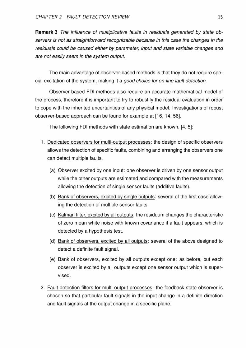
Remark 3 The influence of multiplicative faults in residuals generated by state ob-
servers is not as straightforward recognizable because in this case the changes in the
residuals could be caused either by parameter, input and state variable changes and
are not easily seem in the system output.
The main advantage of observer-based methods is that they do not require spe-
cial excitation of the system, making it a good choice for on-line fault detection.
Observer-based FDI methods also require an accurate mathematical model of
the process, therefore it is important to try to robustify the residual evaluation in order
to cope with the inherited uncertainties of any physical model. Investigations of robust
observer-based approach can be found for example at [16, 14, 56].
The following FDI methods with state estimation are known, [4, 5]:
1. Dedicated observers for multi-output processes: the design of specific observers
allows the detection of specific faults, combining and arranging the observers one
can detect multiple faults.
(a) Observer excited by one input: one observer is driven by one sensor output
while the other outputs are estimated and compared with the measurements
allowing the detection of single sensor faults (additive faults).
(b) Bank of observers, excited by single outputs: several of the first case allow-
ing the detection of multiple sensor faults.
(c) Kalman filter, excited by all outputs: the residuum changes the characteristic
of zero mean white noise with known covariance if a fault appears, which is
detected by a hypothesis test.
(d) Bank of observers, excited by all outputs: several of the above designed to
detect a definite fault signal.
(e) Bank of observers, excited by all outputs except one: as before, but each
observer is excited by all outputs except one sensor output which is super-
vised.
2. Fault detection filters for multi-output processes: the feedback state observer is
chosen so that particular fault signals in the input change in a definite direction
and fault signals at the output change in a specific plane.

CHAPTER 2. FAULT DETECTION REVIEW 16
3. Output observers: another possibility is the use of output observers (unknown
input observers) if the reconstruction of the state variable is not of primary inter-
est. A linear transformation is applied so that the residuals are dependent only
on additive input/output faults.
2.3: Change (fault) detection methods
After the generation of the residuals, it is needed to establish whether there was
a change (fault) on the system or not. This role is done by the change detector which
can be classified under three categories [17]:
1. One model approach: The filter residuals ε(k) are transformed to a distance mea-
sure s(k) (computed from the no-fault values), a stopping rule decide whether the
change is relevant or not. A schematic is show at Figure 2.5.
Figure 2.5: One model approach for change detection
The most natural distance measures are:
• Change in the mean, s(k) = ε(k).
• Change in the variance, s(k) = ε(k)2 − λ, where λ is a known fault-free
variance.
• Change in correlation, s(k) = ε(k)y(k− d) or s(k) = ε(k)u(k− d) for some d.
• Change in sign correlation, s(k) = sign(ε(k)ε(k− 1)), this test is used due to
the fact that white residuals should change sign every second sample in the
average.
2. Two model approach: In this case the residuals are generated by two filters, a
slow (with a great data window or the whole data) and a fast one (with a small data
window) which are compared, Figure 2.6 illustrates the procedure. If the model
based on the smaller data window gives larger residuals a change is detected.
The main problem is to choose an adequate norm for the comparison, typical
norms are:
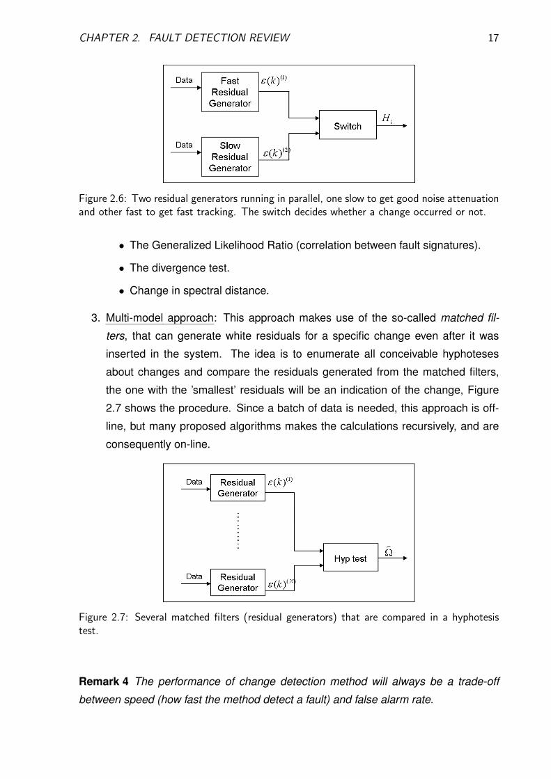
CHAPTER 2. FAULT DETECTION REVIEW 17
Figure 2.6: Two residual generators running in parallel, one slow to get good noise attenuationand other fast to get fast tracking. The switch decides whether a change occurred or not.
• The Generalized Likelihood Ratio (correlation between fault signatures).
• The divergence test.
• Change in spectral distance.
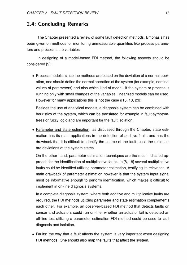
3. Multi-model approach: This approach makes use of the so-called matched fil-
ters, that can generate white residuals for a specific change even after it was
inserted in the system. The idea is to enumerate all conceivable hyphoteses
about changes and compare the residuals generated from the matched filters,
the one with the ’smallest’ residuals will be an indication of the change, Figure
2.7 shows the procedure. Since a batch of data is needed, this approach is off-
line, but many proposed algorithms makes the calculations recursively, and are
consequently on-line.
Figure 2.7: Several matched filters (residual generators) that are compared in a hyphotesistest.
Remark 4 The performance of change detection method will always be a trade-off
between speed (how fast the method detect a fault) and false alarm rate.
CHAPTER 2. FAULT DETECTION REVIEW 18
2.4: Concluding Remarks
The Chapter presented a review of some fault detection methods. Emphasis has
been given on methods for monitoring unmeasurable quantities like process parame-
ters and process state variables.
In designing of a model-based FDI method, the following aspects should be
considered [9]:
• Process models: since the methods are based on the deviation of a normal oper-
ation, one should define the normal operation of the system (for example, nominal
values of parameters) and also which kind of model. If the system or process is
running only with small changes of the variables, linearized models can be used.
However for many applications this is not the case ([15, 13, 23]).
Besides the use of analytical models, a diagnosis system can be combined with
heuristics of the system, which can be translated for example in fault-symptom-
trees or fuzzy logic and are important for the fault isolation.
• Parameter and state estimation: as discussed through the Chapter, state esti-
mation has its main applications in the detection of additive faults and has the
drawback that it is difficult to identify the source of the fault since the residuals
are deviations of the system states.
On the other hand, parameter estimation techniques are the most indicated ap-
proach for the identification of multiplicative faults. In [8, 18] several multiplicative
faults could be identified utilizing parameter estimation, testifying its relevance. A
main drawback of parameter estimation however is that the system input signal
must be informative enough to perform identification, which makes it difficult to
implement in on-line diagnosis systems.
In a complete diagnosis system, where both additive and multiplicative faults are
required, the FDI methods utilizing parameter and state estimation complements
each other. For example, an observer-based FDI method that detects faults on
sensor and actuators could run on-line, whether an actuator fail is detected an
off-line test utilizing a parameter estimation FDI method could be used to fault
diagnosis and isolation.
• Faults: the way that a fault affects the system is very important when designing
FDI methods. One should also map the faults that affect the system.

CHAPTER 2. FAULT DETECTION REVIEW 19
• Performance: fault detectors must be sensitive to the appearance of faults but
insensitive to other changes (noise, operating points, modeling errors, etc.). Be-
cause these requirements often contradict each other, the following trade-offs
must be analyzed:
– size of fault vs detection time;
– speed of fault appearance vs detection time;
– speed of fault appearance vs process response time;
– size and speed of fault vs speed of process parameters changes;
– detection time vs false alarm rate.
Methods that are sensitive to abrupt faults for example, might not be suitable to
detect incipient faults.
• Practical aspects: a FDI method should consider the practical aspects when
defining the experiments to detect the faults, for example safety-critical system,
systems under a closed-loop, network system, etc. and should be robust enough
to cope with them.
• Testing: the introduction of artificial faults is also important to validate the system
reliability and should try to approximate to real faults.

3 State observers
As mentioned in the previous Chapter, one of the most important tasks in a fault
detection scheme is the residual generation method design. A state observer takes
the system input and output signals and utilizing a system model, estimates its states,
which can be used as an analytical redundancy for fault detection.
In this Chapter, we introduce the concept of state observers depicting some of
its properties and different configurations.
3.1: State observers
Given a liner-time invariant system described by the state equations below:
x(k + 1) = Ax(k) +Buu(k)
y(k) = Cx(k) (3.1)
Here x(k) denotes the state vector, u(k) is a known input signal, y(k) are the measured
output signals.
Under the condition that the system is observable (see Section 3.3) and assump-
tions of a known model structure and parameters, the internal state variables x(k) can
estimated with the Luenberger observer:
x(k + 1) = (A− LC)x(k) + L(y(k)) +Buu(k)
y(k) = Cx(k) (3.2)
If system and model parameters are equal, the state error
x(k + 1) = x(k + 1)− x(k + 1)
20
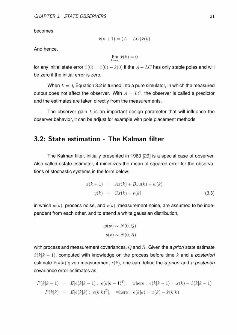
CHAPTER 3. STATE OBSERVERS 21
becomes
x(k + 1) = (A− LC)x(k)
And hence,
limk→∞
x(k) = 0
for any initial state error x(0) = x(0)− x(0) if the A− LC has only stable poles and will
be zero if the initial error is zero.
When L = 0, Equation 3.2 is turned into a pure simulator, in which the measured
output does not affect the observer. With A = LC, the observer is called a predictor
and the estimates are taken directly from the measurements.
The observer gain L is an important design parameter that will influence the
observer behavior, it can be adjust for example with pole placement methods.
3.2: State estimation - The Kalman filter
The Kalman filter, initially presented in 1960 [29] is a special case of observer.
Also called estate estimator, it minimizes the mean of squared error for the observa-
tions of stochastic systems in the form below:
x(k + 1) = Ax(k) +Buu(k) + w(k)
y(k) = Cx(k) + v(k) (3.3)
in which w(k), process noise, and v(k), measurement noise, are assumed to be inde-
pendent from each other, and to attend a white gaussian distribution,
p(w) ∼ N(0, Q)
p(v) ∼ N(0, R)
with process and measurement covariances, Q andR. Given the a priori state estimate
x(k|k − 1), computed with knowledge on the process before time k and a posteriori
estimate x(k|k) given measurement z(k), one can define the a priori and a posteriori
covariance error estimates as
P (k|k − 1) = E[e(k|k − 1) : e(k|k − 1)T ], where : e(k|k − 1) = x(k)− x(k|k − 1)
P (k|k) = E[e(k|k) : e(k|k)T ], where : e(k|k) = x(k)− x(k|k)
CHAPTER 3. STATE OBSERVERS 22
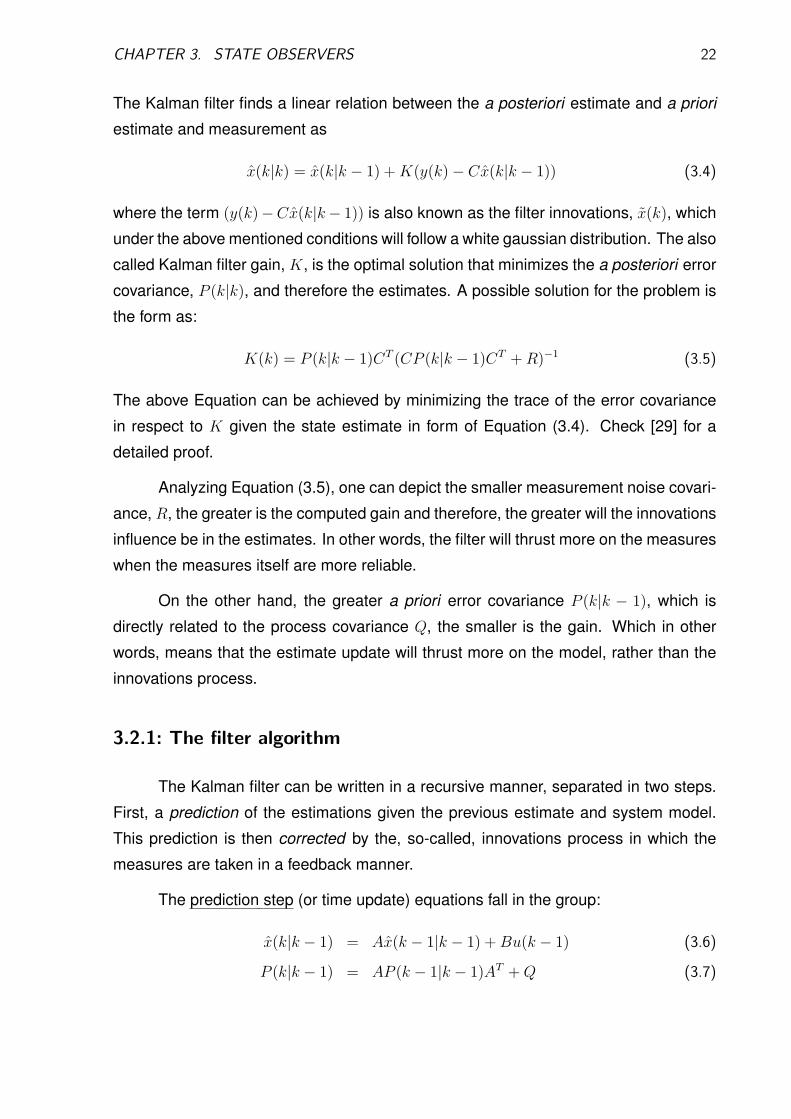
The Kalman filter finds a linear relation between the a posteriori estimate and a priori
estimate and measurement as
x(k|k) = x(k|k − 1) +K(y(k)− Cx(k|k − 1)) (3.4)
where the term (y(k)−Cx(k|k− 1)) is also known as the filter innovations, x(k), which
under the above mentioned conditions will follow a white gaussian distribution. The also
called Kalman filter gain, K, is the optimal solution that minimizes the a posteriori error
covariance, P (k|k), and therefore the estimates. A possible solution for the problem is
the form as:
K(k) = P (k|k − 1)CT (CP (k|k − 1)CT +R)−1 (3.5)
The above Equation can be achieved by minimizing the trace of the error covariance
in respect to K given the state estimate in form of Equation (3.4). Check [29] for a
detailed proof.
Analyzing Equation (3.5), one can depict the smaller measurement noise covari-
ance, R, the greater is the computed gain and therefore, the greater will the innovations
influence be in the estimates. In other words, the filter will thrust more on the measures
when the measures itself are more reliable.
On the other hand, the greater a priori error covariance P (k|k − 1), which is
directly related to the process covariance Q, the smaller is the gain. Which in other
words, means that the estimate update will thrust more on the model, rather than the
innovations process.
3.2.1: The filter algorithm
The Kalman filter can be written in a recursive manner, separated in two steps.
First, a prediction of the estimations given the previous estimate and system model.
This prediction is then corrected by the, so-called, innovations process in which the
measures are taken in a feedback manner.
The prediction step (or time update) equations fall in the group:
x(k|k − 1) = Ax(k − 1|k − 1) +Bu(k − 1) (3.6)
P (k|k − 1) = AP (k − 1|k − 1)AT +Q (3.7)

CHAPTER 3. STATE OBSERVERS 23
In the correction step the actual measurements are used to correct the estima-
tions and filter equations:
K(k) = P (k|k − 1)CT (CP (k|k − 1)CT +R)−1 (3.8)
x(k|k) = x(k|k − 1) +K(k) (y(k)− Cx(k|k − 1)) (3.9)
P (k|k) = (I −K(k)C)P (k|k − 1) (3.10)
The algorithm steps can be translated as:
Prediction(3.6) State prediction given model(3.7) Covariance prediction given model
Correction(3.8) Gain computation(3.9) State correction given innovations
(3.10) Covariance update
Table 3.1: Kalman filter algorithm steps
Finally, an initial guess for P (0) and x(0) is needed. A comparison with the state
observer shown in Section 3.1 shows that the observer only uses past information and
not predicted ones.
Under the assumption of constant Q, R, and model, the gain will converge
quickly and can be pre-computed in an off-line manner solving a Riccati equation of
the error covariance matrix P . In such case the gain is computed as
K = PCT(CPCT +R
)−1
and it can be shown, [5], that, with the prediction inserted, the filter becomes
x(k + 1|k) = Ax(k|k − 1) +Bu(k) + AK (y(k)− Cx(k|k − 1))
which in comparison, is the same as an observer with L = AK.
3.2.2: The extended Kalman filter
The Kalman filter as presented until now is the optimal solution for the state
estimation problem in stochastic linear systems and supposes that both the transition
state matrix A and measurement matrix C to be constant.
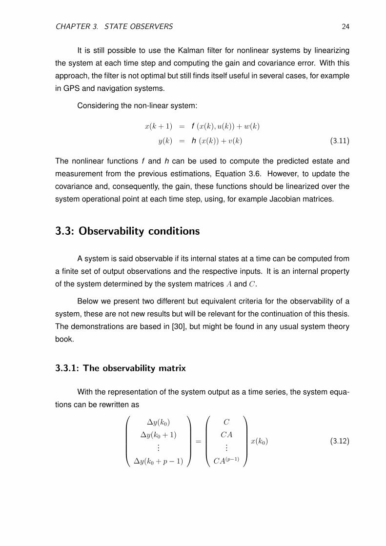
CHAPTER 3. STATE OBSERVERS 24
It is still possible to use the Kalman filter for nonlinear systems by linearizing
the system at each time step and computing the gain and covariance error. With this
approach, the filter is not optimal but still finds itself useful in several cases, for example
in GPS and navigation systems.
Considering the non-linear system:
x(k + 1) = f (x(k), u(k)) + w(k)
y(k) = h (x(k)) + v(k) (3.11)
The nonlinear functions f and h can be used to compute the predicted estate and
measurement from the previous estimations, Equation 3.6. However, to update the
covariance and, consequently, the gain, these functions should be linearized over the
system operational point at each time step, using, for example Jacobian matrices.
3.3: Observability conditions
A system is said observable if its internal states at a time can be computed from
a finite set of output observations and the respective inputs. It is an internal property
of the system determined by the system matrices A and C.
Below we present two different but equivalent criteria for the observability of a
system, these are not new results but will be relevant for the continuation of this thesis.
The demonstrations are based in [30], but might be found in any usual system theory
book.
3.3.1: The observability matrix
With the representation of the system output as a time series, the system equa-
tions can be rewritten as
∆y(k0)
∆y(k0 + 1)...
∆y(k0 + p− 1)
=
C
CA...
CA(p−1)
x(k0) (3.12)

CHAPTER 3. STATE OBSERVERS 25
where ∆y(k) represents all know terms, function of the measured output y(k) and input
u(k):
∆y(k0) = y(k0)−Du(k0)
∆y(k0 + 1) = y(k0 + 1)− CBu(k0)−Du(k0 + 1)
∆y(k0 + 2) = y(k0 + 2)− CABu(k0)− CBu(k0 + 1)−Du(k0 + 2)...
∆y(k0 + p− 1) = y(k0 + p− 1)− CA(p−2)Bu(k0)− . . .−CBu(k0 − p− 2)−Du(k0 + p− 1)
Equation 3.12 has a unique solution for x(k0) if and only if the matrix that multiplies
x(k0) has the same rank as the n total states in the system.
The Cayley-Hamilton theorem, shows that any matrix An linearly depend on
I, A, . . . , A(n−1) (see [30] for a proof), and therefore the criteria can be checked directly
from the matrix:
O =
C
CA...
CA(n−1)
(3.13)
The matrix O is known as the observability matrix and shows that the system is ob-
servable if
rank O = n
Which is equivalent to check if O has full column rank since it has n columns.
3.3.2: The Popov-Belevitch-Hautus criteria
Another important criteria for testing the observability of systems is known as the
Popov-Belevith-Hautus criteria (PBH), firstly studied by these authors. The test depicts
a pair (A C) to be observable if and only if
rank
(C
A− sI
)= n ∀s (3.14)
Where n is the dimension of A. It is easy to see that these conditions are met for all
s that are not eigenvalues of A. The relevance of the theorem is that the rank must

CHAPTER 3. STATE OBSERVERS 26
be n even when s is an eigenvalue of A. For a proof and more insights on system
observability and its dual, controllability, the reader is advised to check [49].
3.4: Concluding remarks
This brief Chapter presented a review on state observers and state estimators
(Kalman filter) as well as relevant observability conditions. The theory of observers
has developed mainly in the 60’s and has been, since then, used successfully in both
industry and academy, specially the (optimal) Kalman filter is applied in different areas
and is still an important tool. The Kalman filter was first designed for linear systems,
and with such constrain, it is actually optimal. For non-linear systems, approaches as
the Extended Kalman filter may work considerably well, but there is no guarantee on
optimality.
With the theoretical background presented so far, the next Section finalizes this
Part presenting the problem of observer-based fault detection in a more thorough man-
ner, holding a discussion on our primary problem description, fault detection through
integrated sensors.

4 Observer-based fault detection
With the introduction to state observers given in the previous Chapter, we finally
present a framework for residual generation using state observers.
We present both the classical approach for residual generation through state ob-
servers (when the raw measurements are available) and the problem that arises when
these measurements are not available but only an estimated output. Such situation
is common in many more advanced sensors where raw measurements are internally
processed before refined information is provided to the user.
The problem of fault detection (mostly related here to the residual generation
task) is studied in both the classical and in the case of observer-integrated sensors.
Conditions for fault observability using the concepts found in the previous Chapter are
depicted as well as a discussion on the methods performance and residual analysis.
4.1: Observer-based residual generation - classical approach
Considering the following system description:
x(k + 1) = Ax(k) +Buu0(k) + Fafa(k) (4.1)
where x(k) denotes the states vector, u0(k) is a fault-free input to the system and fa(k)
model actuator fault inputs, treated as unknown.
When the system inputs and outputs are measured through sensors, which can
also be subject to additive faults as
u(k) = u0(k) + Fufu(k) (4.2)
y(k) = Cx(k) + Fyfy(k) (4.3)
we can use the measured u(k), y(k) and a system model to design a state observer
27

CHAPTER 4. OBSERVER-BASED FAULT DETECTION 28
(see earlier Chapter) as
x(k + 1) = (A− LC)x(k) + L(y(k)) +Buu(k)
y(k) = C∗x(k) (4.4)
where C∗ depicts which estimates are available. The output of the observer y(k) can
then be used to generate a residual ε(k) that is the difference between observer and
system output
ε(k) = y(k)− y(k)
which can be used for fault detection purposes. This is the classical approach for
residual generation through observers. Section 4.1.1 presents some analysis on fault
observability while Section 4.1.2 analyzes the residual behavior.
4.1.1: Fault observability
As described in [55], stochastic biases in linear time invariant systems can be
identified by augmenting the system state with a bias and implement a Kalman filter.
The author utilizes this technique to identify biases in noisy measurements.
In Chapter 3 in [52] these results are extended to check the observability of
additive faults with the constraint that f(t+ 1) = f(t) (faults moving as a random walk).
The faults fa and fy are augmented in the system states, so that we have
x =[x fa fy
]T
A =
A Fa 0
0 I 0
0 0 I
C =[C 0 Fy
](4.5)
Given that the pair (A,C) is observable, the author depicts that the augmented system
observability is provided by checking the rank of the matrix(
C Fy
(A− I) Fa
)
It is also shown that for the especial cases when only measurement or process fault
are present we have the especial conditions:

CHAPTER 4. OBSERVER-BASED FAULT DETECTION 29
• For output measurement faults only (fy)
If the system has no integrator dynamics, the faults will be observable as long
as Fy is full rank.
If there is an integrator in the system dynamics, then the system is not observ-
able if Fy is full column rank and the faults should be orthogonal to the measured
integrating part of the system (modes with eigenvalue equals to 1).
• For process faults only (fa)
Changes introduced by the dynamics of the system which are not directly
measured must be distinguishable (orthogonal) to the disturbances.
In Section 4.2.1 this approach is used to analyze the fault observability for sys-
tems with observer-integrated sensors where the conditions are presented in a more
thorough manner.
4.1.2: Residual analysis
Assuming zero as initial conditions, with C∗ = C and q as the time shift operator,
the observer as in Equation 4.4 can be rewritten in an input output form
y(k) = CH(A−LC)Bu u(k) + CH(A−LC)L y(k)
where HM = [qI −M ]−1
HM is also known as the matrix resolvent ofM and represents the dynamics introduced
by M . The residual is then
ε(k) = (I − CH(A−LC)L) y(k)− CH(A−LC) u(k)
Using Equations (4.1)-(4.3) we can finally write the residual as function of u0(k) and
faults
ε(k) =[(I − CH(A−LC)L)CHA − CH(A−LC)
]Bu u0(k)
+[(I − CH(A−LC)L)CHA
]Fa fa(k)
+[(I − CH(A−LC)L)
]Fy fy(k)
+[−CH(A−LC)Bu
]Fu fu(k) (4.6)
Also, using the matrix identity below

CHAPTER 4. OBSERVER-BASED FAULT DETECTION 30
Theorem 5
A−1 −B−1 = A−1(B − A)B−1
Proof:
A−1 −B−1 = A−1 −B−1
= A−1BB−1 − A−1AB−1
= A−1(BB−1 − AB−1)
= A−1(B − A)B−1
we can show that[(I − CH(A−LC)L)CHA − CH(A−LC)
]= 0, meaning that the residual
is not influenced by the system input, only by the faults. Note that we are not consid-
ering noise and model uncertainties.
This is a very important property for the observer based residual and the faults
will appear in the residual governed by the observer and system dynamics as described
in Equation (4.6).
4.1.2.1: Fault sensitivity
As presented in [30], the sensitivity of the residual to a fault is a transfer function
relating a fault to the residual
Sf (q) =∂ε
∂f
These functions are easily seem in Equation (4.6). We will analyze them as a function
of the observer gain L. The results are related to [50] in which the observer gain is
analyzed for linear interval models (models including uncertainties in the parameters).
For additive input sensor faults we have
Sfu(q) = −CH(A−LC)Bu Fu (4.7)
= −C [qI − (A− LC)]−1Bu Fu

CHAPTER 4. OBSERVER-BASED FAULT DETECTION 31
Analyzing its value at instant times k = 0 and k →∞ we have
Sfu(0) = limq→∞
Sfu(q) = 0 (4.8)
Sfu(∞) = limq→1
Sfu(q)
= −C [I − (A− LC)]−1Bu Fu (4.9)
Showing that at time instant k = 0 the fault is not visible, which is due to the fact that the
fault needs to travel through the observer dynamics before it is visible in the output. We
also depict that the value of the fault in steady state is larger than at the initial instant,
that is
‖Sfu(∞)‖ > ‖Sfu(0)‖ (4.10)
and evolves as a function of the observer dynamics only. We can also check the
influence of the gain in steady-state for two extreme cases. The simulator, L = 0, and
the predictor, LC = A, configurations.
Sfu(∞)|L=0 = −C [I − A]−1Bu Fu (4.11)
Sfu(∞)|LC=A = −CBu Fu (4.12)
Considering a positive A (all its elements positive) and a stable observer with ‖L‖ > 0,
can compare Equations (4.9), (4.11) and (4.12) to conclude
‖Sfu(∞)|L=0‖ > ‖Sfu(∞)|0<LC<A‖ > ‖Sfu(∞)|LC=A‖ (4.13)
The condition above is related to the fact that ‖[qI − (A − LC)]‖ ≥ 1 for any stable
observer. Which comes from the fact that for any consistent norm, such that ‖AB‖ ≤‖A‖ · ‖B‖, we have [53]:
Theorem 6
‖HM‖ =∥∥(sI −M)−1
∥∥ ≥ 1
min1≤i≤n
|s− λi|
Proof: Let (λi, v) be an eigenvector-value pair of M , then:
(sI −M)v = sv −Mv = (s− λi)v
showing that (s− λi) is an eigenvalue of (sI −M). (s− λi)−1 is then an eigenvalue of
(sI −M)−1 finally, since for any consistent norm |λ| ≤ ‖M‖, we have:
max1≤i≤n
1
|s− λi|≤ ‖(sI −M)−1‖

CHAPTER 4. OBSERVER-BASED FAULT DETECTION 32
whence
‖HM‖ = ‖(sI −M)−1‖ ≥ 1
min1≤i≤n
|s− λi|
A physical interpretation of Theorem (6) is that the eigenvalue measures the gain of
a matrix only in one direction (given by eigenvectors) and must be smaller than for
the whole matrix which allows any direction [60]. The norm of the resolvent matrix∥∥(qI −M)−1
∥∥ has, in fact, its lowest bound as 1min
1≤i≤n|s−λi| .
Since the observer is considered stable, we have that all its eigenvalues are
smaller than 1, λA−LCi < 1, depicting a relation to the norm and the eigenvalues of
M . As faster it becomes (smaller eigenvalues), the smaller becomes ‖Sfu‖ (worst
case when LC = A, observer configured as a predictor). Notice that this is just an
indication, the resolvent norm will vary, for example, with frequency.
The above condition gives some insights on the effect of the observer gain L.
Because the predictor configuration uses the measurements directly in the estima-
tions, these estimations will be contaminated by the fault very quickly (depending on
the system order), while in the observer case, the estimations are balanced with the
observer dynamics. Ultimately, for the simulator case, no measurements are used and
the sensitivity function is directly taken by its dynamics in the system.
For additive process faults the sensitivity function is
Sfa(q) =(I − CH(A−LC)L
)CHA Fa
=(I − C [qI − (A− LC)]−1 L
)C [qI − A]−1 Fa
Which can be simplified using Theorem (5) as
Sfa(q) =(I − CH(A−LC)L
)CHA Fa
=(CHA − CH(A−LC)LCHA
)Fa
= C(HA −H(A−LC)LCHA
)Fa
= C(HA +H(A−LC) −HA
)Fa
= CH(A−LC) Fa
(4.14)

CHAPTER 4. OBSERVER-BASED FAULT DETECTION 33
Which depicts that though fa affects the states of the system, it appears in the residual
only as a function of the observer dynamics. And has a similar form as Sfu, but with
opposing signals.
Similarly to an additive input fault, fa will only be visible after a short interval and
dependent only on the observer dynamics since the system dynamics does not affect
fa. The remain analysis follows similar to Sfu(q).
For additive output sensor faults we have
Sfy(q) =(I − CH(A−LC)L
)Fy
=(I − C [qI − (A− LC)]−1 L
)Fy
Analyzing its value at instant times k = 0 and k →∞ we have
Sfy(0) = limq→∞
Sfy(q) = Fy (4.15)
Sfy(∞) = limq→1
Sfy(q) =(I − C [I − (A− LC)]−1 L
)Fy (4.16)
Showing that at time k = 0, it is independent of L and that the value of the fault in
steady state is smaller than at the initial instant and is a function of the observer gain
and its dynamics only. With ‖L‖ > 0 we have ([50])
‖Sfy(∞)‖ < ‖Sfy(0)‖ (4.17)
Checking the influence of the gain,
Sfy(∞)|L=0 = Fy (4.18)
Sfy(∞)|LC=A = limq→1
Sfy(q)|LC=A = (I − CL) Fy (4.19)
Yielding, for a stable observer with ‖L‖ > 0 and a positive A (all its elements positive):
‖Sfy(∞)|L=0‖ > ‖Sfy(∞)|0<LC<A‖ > ‖Sfy(∞)|LC=A‖ (4.20)

CHAPTER 4. OBSERVER-BASED FAULT DETECTION 34
Moreover, in the especial case where C = I, Sfy(q) can be simplified as:
Sfy(q) =(I − CH(A−LC)L
)Fy
=(I −H(A−L)L
)Fy
=(H(A−L)H−1
(A−L) −H(A−L)L)Fy
= H(A−L)
(H−1
(A−L) − L)Fy
= H(A−L)H−1A Fy
= H(A−LC)H−1A Fy (4.21)
The result of the simplification in Equation (4.21) shows (using Theorem (6)), that Sfyis related to the relative speed of the observer (eigenvalues of A − LC) and system
(eigenvalues of A). That is, if the observer is faster than the system indicates, ‖Sfy‖ <‖Fy‖, conversely, if system has faster dynamics would cause ‖Sfy‖ > ‖Fy‖ and if they
are equal (L = 0 for instance) ‖Sfy‖ = ‖Fy‖.
4.1.2.2: Some remarks
Observe that fu and fa have similar effects in the residual (check Equations
(4.14) and (4.8)). Both are dependent only on the observer dynamics but affect the
residual in opposite directions, that is, if fa and fu are affecting the same state, for
example Fa = BuFu, and growimg in the same direction, their effects in the residual will
be opposing to each other and with same value.
Moreover, notice that the simplification for deriving Sfa in Equation (4.14) implies
a perfect system model while Sfu was derived directly and the user should be careful
when analyzing it in a practical situation.
4.2: Observer-based residual generation through integratedsensors
The previous approach requires the availability of y(k). As pointed in the intro-
ductory Chapter, a sensor output might be provided only after the raw measurements
have been internally processed. Here, we will approach this problem with the simplifi-
cation that such sensors are integrated with standard obsevers/Kalman filters.
The idea is to model the sensor as an augmented system model that includes
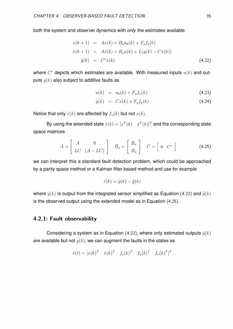
CHAPTER 4. OBSERVER-BASED FAULT DETECTION 35
both the system and observer dynamics with only the estimates available
x(k + 1) = Ax(k) +Buu0(k) + Fafa(k)
x(k + 1) = Ax(k) +Buu(k) + L(y(k)− Cx(k))
y(k) = C∗x(k) (4.22)
where C∗ depicts which estimates are available. With measured inputs u(k) and out-
puts y(k) also subject to additive faults as
u(k) = u0(k) + Fufu(k) (4.23)
y(k) = Cx(k) + Fyfy(k) (4.24)
Notice that only x(k) are affected by fu(k) but not x(k).
By using the extended state x(k) = [xT (k) xT (k)]T and the corresponding state
space matrices
A =
[A 0
LC (A− LC)
]Bu =
[Bu
Bu
]C =
[0 C∗
](4.25)
we can interpret this a standard fault detection problem, which could be approached
by a parity space method or a Kalman filter based method and use for example
ε(k) = y(k)− ˆy(k)
where y(k) is output from the integrated sensor simplified as Equation (4.22) and ˆy(k)
is the observed output using the extended model as in Equation (4.25).
4.2.1: Fault observability
Considering a system as in Equation (4.22), where only estimated outputs y(k)
are available but not y(k), we can augment the faults in the states as
x(t) = [x(k)T x(k)T fa(k)T fy(k)T fu(k)T ]T

CHAPTER 4. OBSERVER-BASED FAULT DETECTION 36
with the resulting matrices
C =[
0 C∗ 0 0 0]
(4.26)
A =
A 0 Fa 0 0
LC (A− LC) 0 LFy BuFu
0 I
(4.27)
we can now analyze the observability for such system when considering faults as driven
by the random-walk, f(k + 1) = f(k). We summarize the results first and present a
more detailed proof in the sequence.
Given that the original pair (A,C) is observable, if the followings conditions are
met:
1. All estimates are available and distinguishable (C is full column rank, for instance,
C∗ = I).
2. L is full column rank, such that
Lz = 0 ⇒ z = 0
the extended system observability can be tested by checking the rank of the matrix(
(A− I) Fa 0 0
LC 0 LFy BuFu
)
which has a similar form as for the case when the actual measurements are available.
This can be explained by the fact that the conditions on the gain and state availability
provides the same information as when we have access to the raw measurements.
The same conditions for process and sensor output faults are achieved as for
the usual case. While input sensor faults fu follows similar conditions as fy:
• For measurement faults only (fy or fu)
If the system has no integrator dynamics, the faults will be observable as long
as Fy (or BuFu) is full rank.
If there is an integrator in the system dynamics, then the system is not ob-
servable if Fy (or BuFu) is full column rank and the states through which the fault

CHAPTER 4. OBSERVER-BASED FAULT DETECTION 37
propagates should be orthogonal to the measured integrating part of the system
(modes with eigenvalue equals to 1).
• For process faults only (fa)
Changes introduced by the dynamics of the system which are not directly
measured must distinguishable (orthogonal) to the disturbances.
The demonstrations follows below.
Demonstration: We will use the Popov- Belevitch-Hautus (PHB) criteria, as pre-
sented in Chapter 3, to check the augmented system observability. The PHB depicts a
pair (A,C) to be observable if (C
A− sI
)
has rank equals n (the number of states) for all s. We will use the following theorems
Theorem 7 The matrix (A
B
)
has full column rank if NA ∩NB = 0.
Proof: (A
B
)
has full column rank if for any v 6= 0
(A
B
)v =
(Av
Bv
)6= 0
which means that the null spaces of A and B are non-intersecting, or
NA ∩NB = 0
Theorem 8 Given K is full column rank, for any B we have:
NKB = NB

CHAPTER 4. OBSERVER-BASED FAULT DETECTION 38
Proof: Suppose NK = ∅. Such that
Kv = 0 → v = 0
Now, let us check the null space of KB
(KB)w = 0, K(Bw) = 0 → Bw = r ∈ NK → Bw = 0
finally, the solution for Bw = 0 is the null-space of B and therefore,
NKB = NB
The faults modes, as shown in Equation (4.27), are s = 1, therefore the analysis will be
separated for s 6= 1 and s = 1.
For s 6= 1 the observability is given by:
0 C∗ 0 0 0
A− sI 0 Fa 0 0
LC (A− LC)− sI 0 LFy BuFu
0 (1− s)I
Following similar simplifications as in [52], we can check that the matrices (1− s)I will
have full rank and with row operations (rank conserving) it can be rewritten as:
0 C∗ 0 0 0
A− sI 0 0 0 0
LC (A− LC)− sI 0 0 0
0 (1− s)I
And therefore, it is sufficient to check the rank of the matrix:
0 C∗
A− sI 0
LC (A− LC)− sI
(4.28)

CHAPTER 4. OBSERVER-BASED FAULT DETECTION 39
which for C∗ full rank, i.e C∗ = I is equivalent to analyze(A− sILC
)
Finally, using Theorem 7 we have the condition that NA−sI ∩ NLC = ∅ which using
Theorem 8 is equivalent toNA−sI∩NC = ∅ which is known to be true since we consider
that the pair (A,C) is observable and the observability for s 6= 1 is achieved.
Notice that last step depicts that the observability is independent on the observer
dynamics in case C∗ is full rank. In case this is not true, C∗ = C for example with C
non full rank, it is possible to find a full column rank L and a pair (A,C) that turns the
system not observable and each case should be considered separately using Equation
(4.28).
Example 9 Take C∗ = C and
A =
(1 1
−2 −2
)C =
(1 0
)L =
(l1
l2
)
Note that we have NA∩NC = ∅ (the system is observable). Considering that analyzing
if a matrix M is full column rank is equivalent to
Mv = 0 ⇔ v = 0
Then, the conditions are achieved by checking Equation (4.28) (with s = 0 for instance):
0 C
A 0
LC (A− LC)
(x
y
)= 0
From which we get that LCx + (A − LC)y = 0. Moreover, since we also have that
y ∈ NC and x ∈ NA it is equivalent to analyze x and y for such. To do so, we can
form a basis A which is formed by the eigenvectors of NA, (1 − 1)T for example, and
equivalently take C formed by eigenvectors ofNC , for instance (0 1)T . And the criteria
can be rewritten as
LCAw + (A− LC)Cv = 0
yielding
l1w + v = 0
l2w − 2v = 0

CHAPTER 4. OBSERVER-BASED FAULT DETECTION 40
which only implies w = v = 0 if −2l1 6= l2 and therefore, there is a full column rank L
that makes the system not observable (even when (A− LC) is stable).
For s = 1, the observability matrix is
0 C∗ 0 0 0
A− I 0 Fa 0 0
LC (A− LC)− I 0 LFy BuFu
0 0
and it is equivalent to analyze(A− I Fa 0 0
LC 0 LFy BuFu
)
For process faults only we can analyze(A− I Fa
LC 0
)(x
y
)
and we have the conditions, (A− I)x+Fay = 0 and x ∈ NLC . For a full column rank L,
the last condition can be rewritten as x ∈ NC . And it is equivalent to analyze such x, to
do so we take a basis C formed by the eigenvectors NC and rewrite the first condition
as
(A− I)Cw + Fay = 0
. This condition can only be true if (A − I)C and Fa share image spaces and the
condition on the observability can be rewritten as
R(A−I)C ∩RFa = ∅
Depicting that changes introduced by the dynamics of the system which are not directly
measured must distinguishable (orthogonal) to the disturbances.

CHAPTER 4. OBSERVER-BASED FAULT DETECTION 41
For measurement faults only we can analyze(
(A− I) 0
LC W
)(x
y
)
where W can either relate to input sensor faults (W = BuFu) or output sensor faults
(W = LFy). We have the conditions that x ∈ NA−I and LCx + Wy = 0. The first
condition is true if and only if x is zero or an eigenvector of A with eigenvalue equals to
1. Hence, it is sufficient to analyze such x. Notice, though, that if A has no integrators
(no eigenvalues equals to 1), then the conditions is achieved by checking if W = BuFu
(for input faults) or W = LFy (for output sensor faults) is full column rank.
If there are integrators in A with a basis A formed by the eigenvectors of NA−Ithe condition is rewritten as LCAv +Wy = 0
For fy we have LCAv + LFyy = 0. Which can be rewritten as
RLCA ∩RLFy = ∅
Which means that the system is not observable if LFy is full rank and the states through
which fy propagates should be orthogonal to the measured integrating part of the sys-
tem propagated by L.
For fu we have
RLCA ∩RBuFu = ∅
Which means that the system is not observable if BuFu is full rank and the states
through which fu propagates should be orthogonal to the measured integrating part of
the system propagated by L.
4.2.2: Residual analysis
As proposed in Section 4.2, we can use the extended state space model, with
C∗ = C
A =
[A 0
LC (A− LC)
]Bu =
[Bu
Bu
]C =
[0 C
]

CHAPTER 4. OBSERVER-BASED FAULT DETECTION 42
to design an observer producing a redundancy ˆy
ˆx(k + 1) = (A−KC)ˆx(k) +K(y(k)) + Buu(k)
ˆy(k) = C ˆx(k) where K = [KT1 KT
2 ]T
and use the residual
ε(k) = y(k)− ˆy(k)
to fault detection purposes.
Following similar steps as in Section 4.1.2, we rewrite the residual in an input-
output form yielding
ε(k) =[(I − CHKK
)CHL (I + LCHA)Bu − CHKBu
]u0(k)
+[(I − CHKK)CHLLCHA
]Fa fa(k)
+[(I − CHKK)CHLL
]Fy fy(k)
+[(I − CHKK
)CHLBu − CHKBu
]Fu fu(k) (4.29)
to simplify the notation, we have written
H(A−LC) = HL
H(A−KC) = HK
where
HM = (qI −N)−1
Using the block matrix inversion:
Theorem 10 If A is invertible then:[A B
C D
]=
[A−1 + A−1B∆−1CA−1 −A−1B∆−1
−∆−1CA−1 ∆−1
]
where ∆, known as the Schur complement, is
∆ =(D − CA−1B
)
Proof: found in any linear algebra book, [53] for example.
we can solve HK and show that the term multiplying the fault-free input u0 equals to
zero.

CHAPTER 4. OBSERVER-BASED FAULT DETECTION 43
4.2.2.1: Fault sensitivity
As presented before, we can analyze the transfer functions Sf (q) = ∂ε∂f
from each
fault to the residual in order to analyze how the faults will behave.
For additive input sensor faults we have:
Sfu(q) =[(I − CHKK
)CHLBu − CHKBu
]Fu
= [(I − C
(qI − (A−KC)
)−1K)C (qI − (A− LC))−1Bu
−C(qI − (A−KC)
)−1Bu]Fu
which can be simplified using Theorem 10 and matrix identities to
Sfu(q) = −C∆−1LC (qI − A)−1BuFu
= −C∆−1LCHABuFu (4.30)
where ∆ is the Schur complement of A as
∆ =(qI − (A− LC −K2C) + LC (qI − A)−1K1C
)
=(H−1
(A−LC−K2C) + LCHAK1C)
(4.31)
Equation (4.30) shows that the fu will depend only on the sensor gain L and the aug-
mented states observer and system dynamics. The system dynamics appear because
the sensor is affected by the input fault also which is propagated by the augmented
observer. The sensor dynamics however are compensated with use of the augmented
observer, though, the sensor gain L still affects the residual.
Analyzing Sfu at instant times k = 0 and k →∞ we have
Sfu(0) = limq→∞
Sfu(q) = 0 (4.32)
Sfu(∞) = limq→1
Sfu(q)
= −C[I − (A− LC −K2C) + LC (I − A)−1K1C
]−1
LC (I − A)−1Bu Fu (4.33)
and consequently
‖Sfu(∞)‖ > ‖Sfu(0)‖ (4.34)

CHAPTER 4. OBSERVER-BASED FAULT DETECTION 44
It might be difficult to analyze the influence of the gainK in such residual through
∆. One should notice, for example, that it will be impossible to have KC = A because
C = [0 C] is not full column rank and KC will have the form
KC =
[0 K1C
0 K2C
]
To be feasible to have KC = A would require that the raw measurements, y(k), are
also available.
Some special cases are:
Sfu(∞)|K=0 = −CBuFu (4.35)
Sfu(∞)|K1=0 = −C [I − (A− LC −K2C)]−1
LC [I − A]−1Bu Fu (4.36)
Sfu(∞)|K2=0 = −C[I − (A− LC) + LC (I − A)−1K1C
]−1
LC [I − A]−1Bu Fu (4.37)
Sfu(∞)|K2=−L = −C[I − (A) + LC (I − A)−1K1C
]−1
LC [I − A]−1Bu Fu (4.38)
Sfu(∞)|K2C=−(I−A+LC) = −C[LC (I − A)−1K1C
]−1
LC [I − A]−1Bu Fu (4.39)
Sfu(∞)|K2C=−(I−A+LC),K1=0 = 0 (4.40)
For additive process faults we have:
Sfa(q) =[(I − CHKK)CHLLCHA
]Fa
which can be simplified similarly as for Sfu to
Sfa(q) = C∆−1LC (qI − A)−1 Fa
= C∆−1LCHAFa (4.41)
where ∆ is the Schur complement of A as in Equation (4.31). Which as in the case
when the raw measurements were available, is similar to Sfu with opposite direction.
The remaining analysis follows similarly to Sfu.

CHAPTER 4. OBSERVER-BASED FAULT DETECTION 45
For additive output sensor faults we have:
Sfy(q) =[(I − CHKK)CHLL
]Fy
which can be simplified to
Sfy(q) = C∆−1LFy (4.42)
where ∆ is the Schur complement of A as in Equation (4.31).
It is interesting to notice here that the Sfy is only dependent on the augmented
observer dynamics through ∆ and on the sensor gain L. As occurred with Sfu, and
consequently to Sfa, the augmented observer took away the influence of the sensor
dynamics HL.
Continuing the analysis for initial and steady conditions we have:
Sfy(0) = limq→∞
Sfy(q) = 0 (4.43)
Sfy(∞) = limq→1
Sfy(q)
= −C[I − (A− LC −K2C) + LC (I − A)−1K1C
]−1LFy (4.44)
and consequently
‖Sfy(∞)‖ > ‖Sfy(0)‖ (4.45)
Again, it might be difficult to analyze the behavior of ∆ with K. We can extend the
results presented for fu from Equations (4.35) to (4.40) by noticing that Sfu = Sfy when
Fy = CHABuFu.
4.2.2.2: Some remarks
With the use of the augmented observer, the influence of the sensor dynamics
H(A−LC) is taken away for all Sf .
However, it might be difficult to analyze the influence of the augmented observer
gain K through ∆. K1 will affect the estimation of x (and consequently of x through the
term LC) as it can be seem in the augmented observer matrix A−KC[
A −K1C
LC (A− LC)−K2C
]

CHAPTER 4. OBSERVER-BASED FAULT DETECTION 46
while K2 will affect the estimation of x only. Choosing K1 = 0 would assume a perfect
model for the internal structure of the measurement system, conversely K2 = 0 as-
sumes a perfect model of the sensor. A typical case would be when, in fact, the sensor
is integrated through an observer (such as a Kalman filter or an extended Kalman filter)
while the internal structure of the system is rather complex or nonlinear, in this case,
if we are interested in state estimation for instance, one should choose a large K1 but
small K2.
A great restriction with this approach is that it requires some knowledge of L. In
fact, in case we have little knowledge on L, we can compensate it increasing K2, that
would try to correct its influence. In the next Section we present an approach where no
knowledge at all in L is needed.
4.2.3: Residual generation - Unknown sensor structure
We study now, the case when the observer structure is not given, for example
if L is unknown, we cannot directly use the augmented observer from Equation (4.22)
for fault detection because we cannot build the extended model. To overcome this
problem, let us make two approximations. Looking at the integrated sensor model
x(k + 1) = Ax(k) +Buu0(k) + Fafa(k)
x(k + 1) = Ax(k) +Buu(k) + L(y(k)− Cx(t))
y(k) = C∗x(k)
With both sensor faults
y(k) = Cx(k) + Fyfy(k)
u(k) = Bu (u(k) + Fufu(k))
The first approximation is
L(Cxf (k) + Fyfy(k)) ≈ Ff f(k)
Here
xf (k + 1) = Axf (k) + Fafa(k) (4.46)
and xf (k) is the fault contribution in x(k). Since fi(k) is zero or a constant vector it is
most important that this approximation holds stationary i.e. after transients.

CHAPTER 4. OBSERVER-BASED FAULT DETECTION 47
The second approximation is
L(y(k)− Cx(k)) ≈ v(k)
where v(k) is a white noise process with a certain covariance matrix. This makes sense
from a Kalman filter point of view where the innovations can be viewed as process
noise, v(k) = Lε(k) where ε(k) = y(k)− Cx(k) is a white innovation process.
This leads to the simplified model
x(k + 1) = Ax(k) +Buu(t) + Ff f(k) + v(k)
y(k) = C∗x(k) + e(k) (4.47)
The artificial measurement noise e(k) can be used to cope with unmodeled char-
acteristics of the system. For example, for sensors over a network or with a weak real-
time performance, one can use e(k) to include jitter, missed samples, delays, etc. or to
cope with sensor/system unknown dynamics.
After defining e(k), it can be used to tune a Kalman filter observer for the sys-
tem as in Equation (4.47) and a standard parity space method or Kalman filter based
method can be used to design a fault detection algorithm. For notation reasons, we will
call the above filter a tracker.
4.2.3.1: Residual analysis
A residual defined as
ε(k) = y(k)− y(k) (4.48)
can be used to perform the detection. Here y(k) is the output estimated from an ob-
server tuned from the model in Equation (4.47) and can be represented by the model
x(k + 1) = (A−KtC∗) x(k) +Buu(k) +Kty(k)
y(k) = C∗x(k) (4.49)

CHAPTER 4. OBSERVER-BASED FAULT DETECTION 48
Writing the residual in an input-output form we have
ε(k) =[(I − C∗H(A−KtC)Kt
)CH(A−LC) (I + LCHA)− C∗H(A−KtC)
]Buu0(k)
+(I − C∗H(A−KtC)Kt
)CH(A−LC)LCHAFa fa(k)
+(I − C∗H(A−KtC)Kt
)CH(A−LC)LFy fy(k)
+[(I − C∗H(A−KtC)Kt
)CH(A−LC) − C∗H(A−KtC)
]BuFu fu(k) (4.50)
from which is easy to show that is independent to u0(k) when C∗ = C.
4.2.3.2: Fault sensitivity
We can analyze the fault sensitivity transfer functions in this case for each fault.
We will consider C∗ = C for all the analysis.
For additive input sensor faults we have:
Sfu(q) =[(I − CH(A−KtC)Kt
)CH(A−LC) − CH(A−KtC)
]BuFu
which can be simplified to
Sfu(q) = −CH(A−KtC)LCH(A−LC)BuFu (4.51)
which reveals that it will be sensitive to both sensor and tracker dynamics, but not to
system dynamics.
Analyzing it for initial and steady states:
Sfu(0) = limq→∞
Sfu(q) = 0 (4.52)
Sfu(∞) = limq→1
Sfu(q)
= −C [I − (A−KtC)]−1 LC [I − (A− LC)]−1BuFu (4.53)
yielding
‖Sfu(∞)‖ > ‖Sfu(0)‖ (4.54)
Checking Equation (4.51) and Theorem (6) that the Sfu is related to the speed of the
tracker filter, which will eventually have smaller values as it becomes faster.
Analyzing the tracker gain Kt for some cases we can depict the steady state

CHAPTER 4. OBSERVER-BASED FAULT DETECTION 49
relations
Sfu(∞)|Kt=0 = −C [I − A]−1 LC [I − (A− LC)]−1BuFu (4.55)
Sfu(∞)|Kt=L = −C [I − (A− LC)]−1 LC [I − (A− LC)]−1BuFu (4.56)
Sfu(∞)|KtC=A = −CLC [I − (A− LC)]−1BuFu (4.57)
For additive process faults we have:
Sfa(q) =(I − CH(A−KtC)Kt
)CH(A−LC)LCHAFa
which can be simplified, to
Sfa(q) = CH(A−KtC)LCH(A−LC)Fa (4.58)
and can be analyzed in a similar manner as for an additive input sensor fault, fu.
For additive output sensor faults we have:
Sfy(q) =(I − CH(A−KtC)Kt
)CH(A−LC)LFy
which can be simplified to
Sfy(q) = CH(A−KtC)H−1A H(A−LC)LFy (4.59)
which reveals that it will be sensitive to system, sensor and tracker dynamics. Notice
though that is has a similar form as Sfy when C = I (see Section 4.1.2.1).
Analyzing it for initial and steady states:
Sfy(0) = limq→∞
Sfy(q) = 0 (4.60)
Sfy(∞) = limq→1
Sfy(q)
= C [I − (A−KtC)]−1 [I − A] [I − (A− LC)]−1 LFy (4.61)
yielding
‖Sfy(∞)‖ > ‖Sfy(0)‖ (4.62)
Similarly to Sfy when C = I in Section 4.1.2.1, the value of ‖Sfu‖ will be related to the
relative location of the eigenvalues of the tracker filter, sensor and system.

CHAPTER 4. OBSERVER-BASED FAULT DETECTION 50
We can analyze the influence of Kt for some cases in steady state:
Sfy(∞)|Kt=0 = C [I − A− LC]−1 LFy (4.63)
Sfy(∞)|Kt=L = C [I − (A− LC)]−1 [I − A]
[I − (A− LC)]−1 Fy (4.64)
Sfy(∞)|KtC=A = −C [I − A] [I − (A− LC)]−1 LFy (4.65)
4.2.3.3: Some remarks
The results are similar to when we have access to the raw measurements, with
the inclusion of the tracker dynamics in the fault sensitivity transfer functions.
4.3: Concluding remarks
In this Chapter, we presented some characteristics of observer based residual
generation for fault detection. Special attention was paid for the case when there is
no direct access to the raw measurements y(k), only to the output of an observer-
integrated sensor. y.
We addressed the question on fault observability for both cases and have shown
that under the conditions for sensor gain L and state availability through C∗
1. All estimates are available (for instance, C∗ = I).
2. L is full column rank, such that
Lz = 0 ⇒ z = 0
one will have a similar case as if the original output was available.
In section 4.2 we proposed two solutions for the case when one has only access
to y(k): using an augmented observer which requires knowledge on the sensor gain L
and estimates both sensor and system states; using a regular observer (tracker) with
the sensor output with a simplified model, with this approach, no a priori knowledge on
L is needed.
The fault sensitivities functions for additive faults have been analyzed for
• ε(k): the residual generated when y(k) is available

CHAPTER 4. OBSERVER-BASED FAULT DETECTION 51
• ε(k): the residual generated with augmented observer (requires some knowledge
on L) and only y(k) is available.
• ε(k): the residual generated with tracker observer and only y is available.
We summarize these results in Table 4.1. The reason why ε(k) would be worse than
ε(k) = y(k)− y(k) ε(k) = y(k)− ˆy(k) ε(k) = y(k)− y(k)
Sfu −CH(A−LC)Bu Fu −C∆−1LCHABu Fu −CH(A−Kt)LCH(A−LC)Bu FuSfa CH(A−LC) Fa C∆−1LCHA Fa CH(A−Kt)LCH(A−LC) FaSfy
(I − CH(A−LC)L
)Fy C∆−1L Fy CH(A−Kt)H−1
A H(A−LC) Fy
Pros Straightforward. Goodfault sensitivity. Easyto tune.
Does not require y(k).Simplify the sensor in-fluence in the sensitivityfunctions.
Simple. Easy to tune. Doesnot require L. Does not requirey(k).
Cons Require y(k). Require L. Complex. Dif-ficult to tune.
Influenced by sensor. Low faultsensitivity.
Table 4.1: Comparison of residual generation approaches.
ε is related to the fact that we have the sensor dynamics affecting the fault sensitivity
functions as design invariant while with ε(k) they are affected by the system dynamics
as design invariant, which are slower, therefore increasing the sensitivity function (see
Theorem (6)). For similar reasons we have also that ε(k) would yield a possible best
residual.
Noise and uncertainties The reasoning that the simulator should always be used is
only true when dealing with a perfect system model and no noise, which is not practical.
Nevertheless, it would be advisable to choose lower values for the gain since that would
increase the fault sensitivity. In [30], Chapter 12, the author presents a more detailed
discussion on modeling errors, how they affect the residual relative to input u(k) (first
order error effect) and to the faults fi(k) (second order error effect).
Optimal residual and the observer design The problem of selecting the gain of the
observer is actually an optimization problem where we would like to have the least in-
fluence of model uncertainties and disturbances in the residual with the most sensitivity
to faults. The way faults, noise and model disturbances affect the system is usually dif-
ferent. It is expected that noise, for example, would appear with low power and high fre-
quency, while model disturbances with an average power and low frequencies. These

CHAPTER 4. OBSERVER-BASED FAULT DETECTION 52
information are important and can be used to design the residual generator. However,
it might be difficult or even impossible to quantify/estimate the effects of these variables
in the output.
Optimal residual generation is a live research topic in the research community,
see for example [56, 57, 58, 59]. In [56], the author presents closed form solutions for
the optimal residual generator in relation to disturbances, however, it requires enough
information on disturbances and faults (a perfect model). A main limitation common to
the techniques developed so far is that the faults need to be directly contained in the
output y(k). In other words, considering the model
x(k + 1) = Ax(k) +Buu(k) +Bdd(k) +Bff(k)
y(k) = Cx(k) +Duu(k) +Ddd(k) +Dff(k)
would recquire Df to be full column rank ([56], page 18). This is usually not the case
for process faults and in case we only have the output from a sensor integrated with an
observer,
x(k + 1) = (A− LC)x(k) +Buu(k) + Ly(k,d, f)
y(k) = Cx(k) +Duu(k)
this will never be the case, since the faults appear through the observer dynamics in
the output y(k).
Kalman filtering Notice that the application of a Kalman filter for fault detection
is similar to the one with an observer. As shown in the previous Chapter, under the
assumptions of constant known noises covariances and model, the Kalman filter is
analogous to an observer with L = AKo, where Ko is the Kalman filter gain. Its use
is specially suitable for systems with large noise since it will attenuate its influence,
however it demands the user extra information about the system and sensors.

Part II
Application example
53

5 Wheeled Mobile robots
A wheeled mobile robot (WMR) is an automatic machine that is capable to move
within an environment utilizing wheels for this purpose. As illustrated in Figure 5.1,
WMRs finds a very wide range of applications in both industry and service, with very
different demands.
Figure 5.1: A container AGV, a robot car, aan utomated vacuum cleaner and a multi-purposemobile platform illustrates the wide range of applications of mobile robots.
Independent of the robot structure and wheel configuration, the task of localiza-
tion is crucial. This is probably still the biggest challenge for the research community
in the area and there has been several improvements and development of different
methods and sensors to achieve this task. So far, the main focus has been in the im-
provement of sensors accuracy and reliability of the methods. It is a great challenge for
any localization method to deal with unexpected changes/conditions in both environ-
ment and robot. Localization reliability can be improved by adding constraints to the
environment the robot interacts with, for example restricting a robot use to even floor,
with a drawback of restricting its application.
Fault/change detection can be used to improve these systems reliability with
relaxed operational constraints. By detecting a fault in the localization system of the
robot, its consequences can be attenuated, increasing the system robustness. In the
past decades, there has been an increased interest in change detection methods for
54

CHAPTER 5. WHEELED MOBILE ROBOTS 55
mobile robots, for example [31, 32, 1]. The field, however, is comparatively recent in
the mobile robots research community with a lot of space for improvements.
In this work we discuss observer-based fault detection for WMR localization sys-
tems. As in any model-based detection framework, the understanding of the system
is crucial. In this Chapter, we present both WMR modeling and localization methods
characteristics. We focus our analysis in differential wheel drive robots and in odome-
try and scan matching localization methods which will provide an introduction to main
challenges to the problem and to the following Chapter which presents a localization
fault detection framework and provide some comparative analyses.
5.1: Robot modeling
A mobile robot is a complex system where the dynamics and kinematics aspects
are very important to its general performance. Different models are required according
to different robot structures and applications. Though kinematic models have been suc-
cessfully used in several applications, for fast moving robots, such as cars, dynamical
models are crucial for performance increase.
Different robot structures will, obviously, require different models. The usual
approach to model a robot mobility is to analyze the contribution of each wheel to its
motion [33]. Active wheels enable the robot to move but also add constraints to the
motion (for example, a car can not move in a 0 radius circular path).
In this work we will only consider a simple kinematic model, assuming the robot
as a rigid body moving in a horizontal plane. The Figure below illustrates the robot in a
global reference frame, where θ is the orientation of the robot relative to the reference
frame, [uf uw]T are the forward and rotational velocities of the robot in respect to its
own frame. It is easy to show the following relation between the robot position and
orientation in the place, called here as pose, [x y θ]T , and its directional speeds,
[uf uw]T :
x
y
θ
t+1
=
x
y
θ
t
+
T cos(θ) 0
T sin(θ) 0
0 T
t
[uf
uw
]
t
(5.1)
where T is the sampling period. Though this model is a rough approximation, it will be
enough for the use within the scope of this thesis. For a more thorough modeling, the

CHAPTER 5. WHEELED MOBILE ROBOTS 56
Figure 5.2: A mobile robot in a reference frame.
reader is advised to check the vast literature on vehicle modeling, [34] for example.
For a differential wheel drive robot, the following relation can be depicted be-
tween the directional speeds [uf uw] and the wheel speeds:[uf
uw
]
t
=
[rR2
rL2
rRb
rLb
]
t
[wR
wL
]
t
(5.2)
where b is the distance between wheels along their common axis, ri and wi are the
wheel radius and wheel rotational speed at side i. This model consider the parameters
ri and b to be constant and, also common, with rR = rL, these are simplifications that
the wheels and chassis are rigid with only one contact point to the ground.
5.2: Pose providers
There are several sensors/methods available to estimate a robot pose, from sim-
ple odometry to Global Positioning Systems (GPS). One might argue that with the ad-
vent of global positioning systems such as GPS, the localization problem is now solved,
this reasoning is partly true and, in fact, such sensors play a significant role in solving
the problem. However, the achieved accuracy for a GPS may vary from centimeters to
tenths of meters (depending, amongst other factors, on atmospheric conditions) which
is unviable in more demanding applications such as service robots.
The Figure below, extracted from [35] gives a scaling perspective of the several
different pose providers methods/sensors:
In the following Section we explore two of the several available methods available

CHAPTER 5. WHEELED MOBILE ROBOTS 57
Figure 5.3: Pose providers methods/sensors in a navigation scale.
for pose estimation. At first, odometry, calculated from wheel speeds rotation is ana-
lyzed, followed by scan matching. A discussion on the error sources and challenges
with the methods is also held.
5.3: Odometry
Odometry was one of the first localization methods developed historically and is
still important for its simplicity, low cost and good short-term accuracy.
The position estimations are achieved by first solving the robot kinematics
from wheel speeds to directional speeds using a kinematics model such as found in
Equation (5.2) for a differential drive robot. With the estimates uf and uw, and given an
initial pose, it is possible to achieve an estimate of the current pose through the model
presented in Equation (5.1).
The velocity can be measured in several different manners. A common and very
usual one is the use of optical encoders. As presented in Figure 5.4, such devices,
when coupled to a rotating axis, estimate velocity by checking the time interval between
consecutive blanks seen by a photo sensor. There are several different configurations
for the device with increased accuracy depending on the number of ticks in the en-
coder wheels and the clock speed. For the application in mobile robots, the errors with
these measures remain bounded and in a much smaller range when compared to other
uncertainty sources and are often assumed to be insignificant [33].
5.3.1: Error sources
Odometry is based on the assumption that wheel revolutions can directly relate
to linear displacements, for example, Equation (5.2) presents such relations for a dif-
ferential drive robot. This model is only valid under some simplifications such as a
robot moving in a fixed plan, a constant and unique contact point to the wheels, perfect
alignment of wheels and so on. These simplifications and other stochastic effects may

CHAPTER 5. WHEELED MOBILE ROBOTS 58
Figure 5.4: Optical encoder scheme. Extracted from the Wikipedia.
and will lead to errors in the odometry readings.
The errors can be categorized under two groups, systematic and random er-
rors. Systematic errors are caused by known sources and/or assumptions that can be
(sometimes) easily handled, some examples:
• Error introduced by uneven wheel radii.
Caused for example by a badly calibrated tire.
• Actual wheelbase differing from nominal (used to solve the odometry equations).
Caused for example by the use of a thick inflatable tire with several and not
constant contact point to the ground.
• Misalignment of wheels.
Introduced by a bad mechanical design or fatigue caused by extensive use.
• Finite wheel encoder resolution and finite sampling rate.
A wheel encoder based sensor measures a discrete quantity and therefore
resolution and sampling rate should be considered.
While most of the systematic error can be reduced with a better calibration of
the system (see [36] for an example), there are other sources of error that affect the
system in a stochastic manner and cannot be compensated for in a predictive manner,
some examples:
• Travel over uneven floors.
Should be faced in any outdoor application in which the robot path may vary
considerable.

CHAPTER 5. WHEELED MOBILE ROBOTS 59
• Unexpected interaction with other entities.
A common situation for robots that are designed to interact with people, when
someone may push it away for example.
• Wheel slippage.
There are several causes for wheel slippage: overacceleration of the wheels,
driving over slippery floors, forces due to the castor wheels, skidding, etc.
Depending on where the robot is being operated, systematic errors can be less
or more important to the overall performance of the robot. For example, if the robot
is traveling in a flat and clean floor, the systematic errors will be much larger than the
random ones.
5.3.2: Error modeling
A good understanding of the errors evolution, causes and behavior is of great
relevance for the localization task as well as for a detection scheme. There has been
several efforts in modeling odometry errors, [33, 37, 38], a model for odometry errors
is very important in allowing sensor fusion techniques and the use of Kalman filter
observers.
In [33], for example, the equations for the covariance error matrix of odometry
are derived for differential drive robots by considering piecewise travel motions up-
dated according to a kinematics robot model, Equation (5.1), and robot mobility model,
Equation (5.2). The incremental traveled distances are:
pt+∆t =
x
y
θ
t+∆t
=
x
y
θ
t
+
∆s cos(θt + ∆θ2
)
∆s sin(θt + ∆θ2
)
∆θ
(5.3)
with
∆θ =∆sR −∆sL
b, ∆s =
∆sR + ∆sL2
where ∆si is the traveled distance at side i. The final odometry position update is then
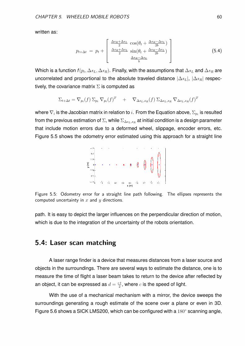
CHAPTER 5. WHEELED MOBILE ROBOTS 60
written as:
pt+∆t = pt +
∆sR+∆sL
2cos(θt + ∆sR−∆sL
2b)
∆sR+∆sL
2sin(θt + ∆sR−∆sL
2b)
∆sR−∆sL
b
(5.4)
Which is a function f (pt,∆sL,∆sR). Finally, with the assumptions that ∆sL and ∆sR are
uncorrelated and proportional to the absolute traveled distance |∆sL|, |∆sR| respec-
tively, the covariance matrix Σ is computed as
Σt+∆t = ∇pt(f) Σpt ∇pt(f)T + ∇∆sL,sR(f) Σ∆sL,sR
∇∆sL,sR(f)T
where∇i is the Jacobian matrix in relation to i. From the Equation above, Σpt is resulted
from the previous estimation of Σ, while Σ∆sL,sRat initial condition is a design parameter
that include motion errors due to a deformed wheel, slippage, encoder errors, etc.
Figure 5.5 shows the odometry error estimated using this approach for a straight line
Figure 5.5: Odometry error for a straight line path following. The ellipses represents thecomputed uncertainty in x and y directions.
path. It is easy to depict the larger influences on the perpendicular direction of motion,
which is due to the integration of the uncertainty of the robots orientation.
5.4: Laser scan matching
A laser range finder is a device that measures distances from a laser source and
objects in the surroundings. There are several ways to estimate the distance, one is to
measure the time of flight a laser beam takes to return to the device after reflected by
an object, it can be expressed as d = c t2
, where c is the speed of light.
With the use of a mechanical mechanism with a mirror, the device sweeps the
surroundings generating a rough estimate of the scene over a plane or even in 3D.
Figure 5.6 shows a SICK LMS200, which can be configured with a 180◦ scanning angle,

CHAPTER 5. WHEELED MOBILE ROBOTS 61
Figure 5.6: Laser range finder from SICK.
resolution of 0.5◦ and 10m range, the device takes 4 scans in 1 second. A result of such
scan is shown in Figure 5.7 where 361 points are taken in one scan.
Figure 5.7: 2D laser scan over 180◦. The (0, 0) position coincides to the laser source.
Scan matching consists of estimating the roto-translation relation between two
different scans. Consider, for example, Figure 5.8 where two scans were taken from
a laser range finder mounted in a mobile robot that was rotated clockwise from time
t0 to tk. The scan matching algorithm finds the transform between the scans and
consequently an estimate of how the robot has moved.
There are many algorithms available to perform scan matching. They might differ
considerably from the scope of localization (global or local). Global localization takes
no prior information of the robot position while for local localization some knowledge of
previous estimates are available (from odometry for example).
Scan matching algorithms also differ by the kind of information they look into
the scans in order to find the transform, some algorithms might only compare points in
the scans while others might look at scene features (searching for lines for example),
which in turn requires some assumptions on the environment. In the following Sections

CHAPTER 5. WHEELED MOBILE ROBOTS 62
Figure 5.8: 2D laser scans over 180◦ with a rotation clockwise rotation between them.
we present two approaches for scan matching.
5.4.1: Iterative Closest Point - ICP
As the name points out, this is an iterative method which compares the scans
in a point to point manner. It is one of the most common approaches for local scan
matching and has a wide number of variants. It was first proposed in [40]. Given a
reference, a current scan and an initial estimate of the transform relating them, ICP
consists of the following tasks:
• Transform the new scan using the current estimate of the transformation.
• Selection of some set of points in one or both scans.
Since the robot is moving, some points in the new scan might not even be
seen in the reference scan, choosing which point should be used is therefore
very important.
• Matching the selected points between the scans.
In this task the points selected in one of the scans are corresponded to points
in the other scan.
• Rejecting some of the pairs that might deviate too much.
The matching is not perfect and some pairs should be discarded.
• Updating the transform given the matched points.
The algorithm iterates until it converges to a match exceeding some criteria. There are
several variants of the algorithm, differing in how it solves the above tasks see [39, 41]

CHAPTER 5. WHEELED MOBILE ROBOTS 63
for example. The ICP tries to find the transform, T , that minimizes the total squared
error between the scans.
Tmin = arg minT
1
N
N∑
i=1
‖Tri − s− i‖ (5.5)
where ri and si are points in a reference and a current scan.
Rather than presenting a full proof of the solution of the above equation, we shall
present a simple implementation of the algorithm, based in [40].
Given two scans (R, S) and an initial roto-translation transform T0 between them,
the algorithm iterates in a loop as shown in Algorithm (1) until some criteria is reached.
To simplify some of the calculations one can use an homogeneous transform, including
both rotation and translation in a joint transform as below:
T =
[Rot Trans
0 1
]=
cos(θ) sin(θ) tx
− sin(θ) cos(θ) ty
0 0 1
Algorithm 1 (T ) = match(R, S, T0). Main scan matching loop.
Require: T0 6= 0T = T0
while ∆T > criteria do(S∗) = T × S {apply current transform.}(assoc) = getAssociatons(R, S∗) {get p2p associations between scans.}(R′, S ′) = rejectOutliers(R, S∗, assoc)(∆T ) = getTransform(R′, S ′) {get matching transform.}(T ) = ∆T × T {update transform estimate.}
end whilereturn T
The getAssociatons function simply relates a point in the R scan with the clos-
est point in the S scan, assuring that only one point is associated to another.
Due to changes in the scene between the scans, it could happen that a point in S
is not present in R, the use of such points should be avoided in the matching process.
The function rejectOutliers performs the task of excluding such points. There are
several ways to reject outliers, here we use a very simple approach, taking away points
that are below the median value of the distances of all associations.
Finally, the function getTransform takes the scans and current associations and
return the transform between them.
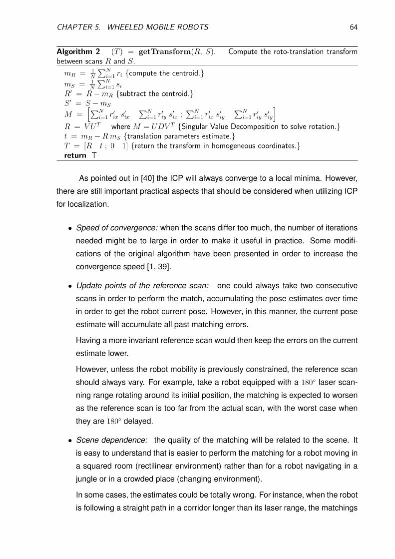
CHAPTER 5. WHEELED MOBILE ROBOTS 64
Algorithm 2 (T ) = getTransform(R, S). Compute the roto-translation transformbetween scans R and S.
mR = 1N
∑Ni=1 ri {compute the centroid.}
mS = 1N
∑Ni=1 si
R′ = R−mR {subtract the centroid.}S ′ = S −mS
M =[∑N
i=1 r′ix s
′ix
∑Ni=1 r
′iy s′ix ;
∑Ni=1 r
′ix s
′iy
∑Ni=1 r
′iy s′iy
]
R = V UT where M = UDV T {Singular Value Decomposition to solve rotation.}t = mR −RmS {translation parameters estimate.}T = [R t ; 0 1] {return the transform in homogeneous coordinates.}return T
As pointed out in [40] the ICP will always converge to a local minima. However,
there are still important practical aspects that should be considered when utilizing ICP
for localization.
• Speed of convergence: when the scans differ too much, the number of iterations
needed might be to large in order to make it useful in practice. Some modifi-
cations of the original algorithm have been presented in order to increase the
convergence speed [1, 39].
• Update points of the reference scan: one could always take two consecutive
scans in order to perform the match, accumulating the pose estimates over time
in order to get the robot current pose. However, in this manner, the current pose
estimate will accumulate all past matching errors.
Having a more invariant reference scan would then keep the errors on the current
estimate lower.
However, unless the robot mobility is previously constrained, the reference scan
should always vary. For example, take a robot equipped with a 180◦ laser scan-
ning range rotating around its initial position, the matching is expected to worsen
as the reference scan is too far from the actual scan, with the worst case when
they are 180◦ delayed.
• Scene dependence: the quality of the matching will be related to the scene. It
is easy to understand that is easier to perform the matching for a robot moving in
a squared room (rectilinear environment) rather than for a robot navigating in a
jungle or in a crowded place (changing environment).
In some cases, the estimates could be totally wrong. For instance, when the robot
is following a straight path in a corridor longer than its laser range, the matchings
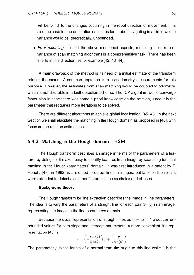
CHAPTER 5. WHEELED MOBILE ROBOTS 65
will be ’blind’ to the changes occurring in the robot direction of movement. It is
also the case for the orientation estimates for a robot navigating in a circle whose
variance would be, theoretically, unbounded.
• Error modeling: for all the above mentioned aspects, modeling the error co-
variance of scan matching algorithms is a comprehensive task. There has been
efforts in this direction, se for example [42, 43, 44].
A main drawback of the method is its need of a initial estimate of the transform
relating the scans. A common approach is to use odometry measurements for this
purpose. However, the estimates from scan matching would be coupled to odometry,
which is not desirable in a fault detection scheme. The ICP algorithm would converge
faster also in case there was some a priori knowledge on the rotation, since it is the
parameter that recquires more iterations to be solved.
There are different algorithms to achieve global localization, [45, 46], in the next
Section we shall elucidate the matching in the Hough domain as proposed in [46], with
focus on the rotation estimations.
5.4.2: Matching in the Hough domain - HSM
The Hough transform describes an image in terms of the parameters of a fea-
ture, by doing so, it makes easy to identify features in an image by searching for local
maxima in the Hough (parameters) domain. It was first introduced in a patent by P.
Hough, [47], in 1962 as a method to detect lines in images, but later on the results
were extended to detect also other features, such as circles and ellipses.
Background theory
The Hough transform for line extraction describes the image in line parameters.
The idea is to vary the parameters of a straight line for each pair (x, y) in an image,
representing the image in the line parameters domain.
Because the usual representation of straight lines as y = ax + b produces un-
bounded values for both slope and intercept parameters, a more convenient line rep-
resentation [48] is
y =
(−cos(θ)
sin(θ)
)x+
(ρ
sin(θ)
)
The parameter ρ is the length of a normal from the origin to this line while θ is the

CHAPTER 5. WHEELED MOBILE ROBOTS 66
orientation of ρ in respect to the abscissas, see Figure 5.9. Finally, the representation
Figure 5.9: (ρ, θ) line parametrization.
can be rewritten as:
ρ = x cos(θ) + y sin(θ) (5.6)
The result of a Hough transform for a selected set of points in a scan can be
seen in Figure 5.10.
(a) Orginal scan (b) After HT
Figure 5.10: Hough transform representation.
If we restrict the θ domain to [0, π), than ρ is unique for a line. Some other
interesting properties of the transform [48]:
• A point in the (x, y) domain corresponds to a sinusoid in the (ρ, θ) domain.
• A point in the (ρ, θ) domain corresponds to a line in the (x, y) domain.
• Collinear points in the (x, y) corresponds to intercepting curves in the (ρ, θ) do-
main.
• Points on the same curve in the (ρ, θ) domain corresponds to lines through the
same point in the (x, y) domain.
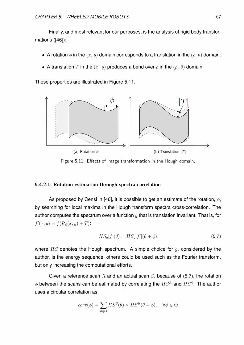
CHAPTER 5. WHEELED MOBILE ROBOTS 67
Finally, and most relevant for our purposes, is the analysis of rigid body transfor-
mations ([46]):
• A rotation φ in the (x, y) domain corresponds to a translation in the (ρ, θ) domain.
• A translation T in the (x, y) produces a bend over ρ in the (ρ, θ) domain.
These properties are illustrated in Figure 5.11.
(a) Rotation φ (b) Translation |T |
Figure 5.11: Effects of image transformation in the Hough domain.
5.4.2.1: Rotation estimation through spectra correlation
As proposed by Censi in [46], it is possible to get an estimate of the rotation, φ,
by searching for local maxima in the Hough transform spectra cross-correlation. The
author computes the spectrum over a function g that is translation invariant. That is, for
f ′(x, y) = f(Rφ(x, y) + T ):
HSg[f ](θ) = HSg[f′](θ + φ) (5.7)
where HS denotes the Hough spectrum. A simple choice for g, considered by the
author, is the energy sequence, others could be used such as the Fourier transform,
but only increasing the computational efforts.
Given a reference scan R and an actual scan S, because of (5.7), the rotation
φ between the scans can be estimated by correlating the HSR and HSS. The author
uses a circular correlation as:
corr(φ) =∑
θ∈Θ
HSS(θ)×HSR(θ − φ), ∀φ ∈ Θ

CHAPTER 5. WHEELED MOBILE ROBOTS 68
Figure 5.12 shows an example of the computed spectrum and its cross-correlation for
two scans.
(a) Original scans (b) Spectrum and cross-correlation (sinusoid likecurve in the background)
Figure 5.12: φ estimation by spectra correlation.
The number of hypotheses generated using this method can be chosen arbitrar-
ily, allowing global localization. The different hypotheses are relevant for example in a
SLAM (simultaneous localization and mapping) context. Here, however, we are only
interested in the pose tracking which is related to the previous estimations, this infor-
mation can be used to restrict the search domain for φ, reducing the computational
efforts.
With the φ hypotheses, it is possible to estimate the translation in several man-
ners, for example using ICP. In [46] the author proposes its estimate in the Hough
domain.
It is important to note that, even though the estimates are taken in the Hough
domain, no assumptions on the scene geometry are needed, but the estimations are
improved for rectilinear environments.
5.4.2.2: Complexity
As shown in [46] the complexity for finding the rotation estimation is
O(Rσφ + φmaxσ
2φ
)
where R are the number of points in the scan, σφ is the required angular discretization
(resolution of the solution) and φmax is a bound for the search of φ. That is, linear in the

CHAPTER 5. WHEELED MOBILE ROBOTS 69
number of data points and quadratic on the resolution.
5.5: Concluding remarks
In this Chapter we have presented some relevant aspects of wheeled mobile
robots, including some approaches to modeling and, most relevant to this work, the
characteristics of two common pose providers. We summarize the relevant results:
In Section 5.1:
• The kinematics model for pose update as in Equation 5.1.
This model, regardless its simplicity, can be used for sensor fusion, for exam-
ple in an Extended Kalman filter.
• The model relating wheel speeds to direction speeds for a differential drive robot.
This model is what is commonly used in pose estimation for odometry and an
analysis of the assumptions in which the model is valid is important to understand
what kind of model disturbances can affect odometry.
In Section 5.3 we explored odometry with a more comprehensive analysis in-
cluding:
• Presentation of its principle of operation.
Giving the reader a general understanding of the instrumentation used in
odometry.
• Discussion on the main error sources.
Very important to help the understanding of the estimates and behavior under
different conditions.
• Discussion on error covariance matrix estimation.
The unbounded error behavior related to the integrative method used in odom-
etry was presented with a simple error modeling. Noticeable is the fact that it in-
creases with the navigation time, with more impact in the direction perpendicular
to the movement.
Finally, Section 5.4 explored the use of laser range finder sensors dealing with
the localization problem, some remarks:

CHAPTER 5. WHEELED MOBILE ROBOTS 70
• Presentation of its principle of operation.
• Description of the Iterative Closes Point (ICP) scan matching algorithm.
This is one of the most common approaches to scan matching and a version
of the algorithm was presented. It has also been pointed out its current main
challenges and a discussion on error modeling.
A remarkable characteristic is its need for an initial transform to perform the
matching with a reasonable convergence speed.
• Method for global estimate of the rotation transform between scans.
We presented a method to estimate scan rotations using the Hough transform
that has a bounded computational complexity. For this purpose we presented the
basics of the Hough transform and its application to scan matching.
The estimate of the rotation with such method can be used, for example, as a
initial guess for an ICP algorithm.
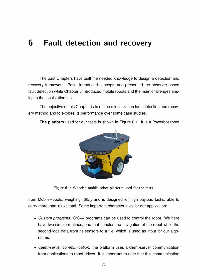
6 Fault detection and recovery
The past Chapters have built the needed knowledge to design a detection and
recovery framework. Part I introduced concepts and presented the observer-based
fault detection while Chapter 5 introduced mobile robots and the main challenges aris-
ing in the localization task.
The objective of this Chapter is to define a localization fault detection and recov-
ery method and to explore its performance over some case studies.
The platform used for our tests is shown in Figure 6.1. It is a Powerbot robot
Figure 6.1: Wheeled mobile robot platform used for the tests.
from MobileRobots, weighing 120kg and is designed for high payload tasks, able to
carry more than 100kg total. Some important characteristics for our application:
• Custom programs: C/C++ programs can be used to control the robot. We here
have two simple routines, one that handles the navigation of the robot while the
second logs data from its sensors to a file, which is used as input for our algo-
rithms.
• Client-server communication: the platform uses a client-server communication
from applications to robot drives. It is important to note that this communication
71

CHAPTER 6. FAULT DETECTION AND RECOVERY 72
is not deterministic and jitters/delays might occur and therefore the sampling rate
will not be constant.
• Differential drive: the robot’s mobility is achieved through two wheels driven by
DC motors and two extra rear caster wheels for balance in an almost holonomic
robot.
The robot uses 25cm diameter inflatable tires. This type of tires requires more
careful when using odometry, since the basic assumptions of constant wheels
radii and one contact point between wheel and floor are weakened. It is then
expected an increase of odometry errors caused by model uncertainties.
The robot is equipped with odometry and a SICK laser range finder which are used to
provide two redundant localization outputs.
Our objective is to detect and attenuate faults causing a bias in the odometry
pose estimation. Two different faults are prioritized:
• Hard faults, caused by external disturbances such as the robot being pushed, that
affects considerably the robot pose, but are not visible in the odometry estimates.
• Slippage faults, that affects the robot positioning but slower and with smaller am-
plitudes. It can be caused for example by a robot navigating in a dusty terrain or
grasping over a wall.
To be able to detect and attenuate these faults, the following Sections present both a
change detection framework and a recovery method that include the detection infor-
mation to attenuate the faults.
6.1: Change detection
Recapitulating from Chapter 2, a change detection takes a set of measured data
from a system, subject to noise/disturbances as well as faults and filters it attempting
to detect a change introduced by a fault. It is subdivided in different tasks:
Figure 6.2: Change detection scheme.

CHAPTER 6. FAULT DETECTION AND RECOVERY 73
• Residual generator: a filter that given a set of measured data provides a residual
ε(k), a quantity that should be sensible to faults but not noise/disturbances.
• Distance measure: is a metric of the changes occurring in the residual, outputs
s(k).
• Stopping rule: a decision making filter that generates alarms in case its input has
exceeded a certain criteria.
We elucidate each of those subtasks in our framework.
6.1.1: Residual generation
This is probably the most important task in a fault detection scheme and is usu-
ally the one that require more design efforts. As shown in Chapter 2, there are different
manners to define a residual generator, our focus here is observer-based residual gen-
eration. We suppose two localization methods (pose providers) are available, odometry
and laser scan matching.
Odometry, podo, is very commonly used as a pose provider. As explained in
the previous Chapter, its pose estimation error grows with the traveled distance in a
non-linear manner. It is successfully used however, if it is possible to reset the errors,
keeping it bounded under a certain region of operation or for short range tasks.
Scan matching, psm, is achieved from a laser range finder installed in the robot.
The algorithm used mixes the rotation estimation in the Hough domain and Iterative
Closest Point, as explained in the previous Chapter.
Since the robot heading φ estimate is the hardest, it is first estimated in the
Hough domain by looking for local maxima in the spectra correlation. This provides
a set of hypotheses for φ which are selected by checking the one that provides the
smallest ∆T in the ICP algorithm (output of function getTransform), check Algorithm
(1). The main advantage of this approach is that we always find a reasonable estimate
of φ, the accuracy of the estimate is related to the resolution of the transform.
Finally, the translation displacements (∆x ∆y) are estimated with the ICP di-
rectly, since we have a good initial guess of φ, we use a 0.5◦ resolution Hough trans-
form, the estimates converge in a couple of iterations of the ICP.

CHAPTER 6. FAULT DETECTION AND RECOVERY 74
Figure 6.3 shows the pose estimations for both scan matching and odometry.
Notice the larger variance from the laser estimates and the difference in the x esti-
mation caused by odometry model errors, easily seem in this example due to a badly
calibrated tire. With the pose providers described, we can introduce the different resid-
Figure 6.3: Output from odometry and laser scan matching.
uals that we will use for comparison reasons here.
6.1.1.1: ε0 - difference between poses
The first one is the usual residual taken as the direct difference between the
redundant sensors. In our case it is defined as
ε0(k) = podo(k)− psm(k)
6.1.1.2: ε - observer with unknown sensor structure
The second residual is based on the tracker filter presented in Section 4.2.3.
In this case, we neglect the sensor dynamics and directly apply an observer/Kalman
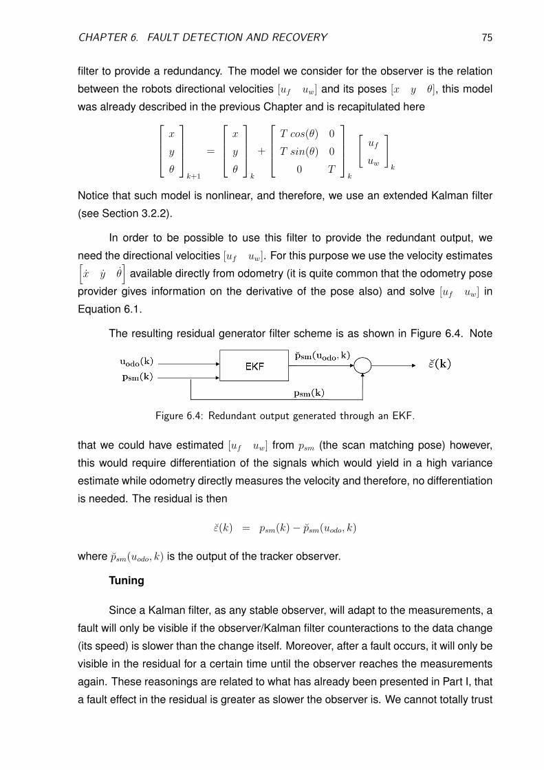
CHAPTER 6. FAULT DETECTION AND RECOVERY 75
filter to provide a redundancy. The model we consider for the observer is the relation
between the robots directional velocities [uf uw] and its poses [x y θ], this model
was already described in the previous Chapter and is recapitulated here
x
y
θ
k+1
=
x
y
θ
k
+
T cos(θ) 0
T sin(θ) 0
0 T
k
[uf
uw
]
k
Notice that such model is nonlinear, and therefore, we use an extended Kalman filter
(see Section 3.2.2).
In order to be possible to use this filter to provide the redundant output, we
need the directional velocities [uf uw]. For this purpose we use the velocity estimates[x y θ
]available directly from odometry (it is quite common that the odometry pose
provider gives information on the derivative of the pose also) and solve [uf uw] in
Equation 6.1.
The resulting residual generator filter scheme is as shown in Figure 6.4. Note
Figure 6.4: Redundant output generated through an EKF.
that we could have estimated [uf uw] from psm (the scan matching pose) however,
this would require differentiation of the signals which would yield in a high variance
estimate while odometry directly measures the velocity and therefore, no differentiation
is needed. The residual is then
ε(k) = psm(k)− psm(uodo, k)
where psm(uodo, k) is the output of the tracker observer.
Tuning
Since a Kalman filter, as any stable observer, will adapt to the measurements, a
fault will only be visible if the observer/Kalman filter counteractions to the data change
(its speed) is slower than the change itself. Moreover, after a fault occurs, it will only be
visible in the residual for a certain time until the observer reaches the measurements
again. These reasonings are related to what has already been presented in Part I, that
a fault effect in the residual is greater as slower the observer is. We cannot totally trust

CHAPTER 6. FAULT DETECTION AND RECOVERY 76
the model (simulator case) though, since then the residual would also be consider-
ably vulnerable to noise/disturbances. The observer tuning is then a tradeoff between
noise/disturbance attenuation and sensitivity to faults.
To tune the EKF we need the measurement and process noise covariance ma-
trices. As depicted in the previous Chapter the advantage of scan matching is that its
errors can be kept bounded within a region. Using fault free data, we could depict our
scan matching variance as
R =
[0.032 0.052
(0.5 ∗ π
180
)2]
that is, a 3cm standard deviation for the x estimates, 5cm for y and 0.5◦ in θ. The
higher variance for y is due to the fact that estimates in the perpendicular direction of
movement are more difficult.
The estimate of the process noise covariance matrix might be difficult, it is re-
lated, amongst other factors, to the robot structure, travel speed, etc. However, since
we would like our filter not to be so fast (giving more relevance to the model estimates
rather than the measurements), we simply consider the process noise as a tenth of our
measurement noise
Q =
[0.0032 0.0052
(0.05 ∗ π
180
)2]
With Q and R set this way, the filter is set and we can use the residual ε(k) to perform
the detection.
6.1.1.3: ε - augmented observer
As discussed in Chapter 4 Section 4.2, another possible approach to achieve
fault detection with integrated/encapsulated sensors is to suppose sensors are inte-
grated with an observer/kalman filter and build a model augmenting the internal sensor
states x =[xT xT
]T with the augmented system matrices
A =
[A 0
LC (A− LC)
]Bu =
[Bu
Bu
]C =
[0 C
]
and use for example an extended Kalman filter with such augmented model to provide
the redundancy. The final structure, shown in Figure 6.5, is similar to the tracker pre-
sented earlier with the difference that we use the augmented states model in the filter.

CHAPTER 6. FAULT DETECTION AND RECOVERY 77
Figure 6.5: Redundant output generated through an augmented observer.
The residual is then
ε(k) = psm(k)− psm(uodo, k)
where psm(uodo, k) is the output of the augmented states observer.
Tunning
The EKF tuning in this case is a bit more comprehensive since the covariance
matrice Q is now doubled in size and we also need to consider the internal sensor
structure, which with our approximation that sensors are integrated with observers, is
actually the sensor gain L.
Here, we are simply going to choose an L that yields an stable observer, that is
λ(A−LC) < 1, ∀ λ
and that has faster dynamics then the system
λ(A−LC) < λA, ∀ λ
notice that since our model is nonlinear, L needs to be solved at each time step with
the linearized model of the system. Since a slower sensor and consequently smaller L
would yield a residual more sensible to a fault we choose an L that makes the observer
speed to be 10% faster than the system
λ(A−LC) = 0.9× λA, ∀ λ
It is expected that the internal sensor states have a greater variance than the
systems’, the matrix Q is so that the sensor states are 2 times larger standard deviation
than the ones available as output
Q =
[0.0032 0.0052
(0.05 ∗ π
180
)2
0.00152 0.00252
(0.025 ∗ π
180
)2]
Since, as previously, we use measurements from the scan matching, R is con-

CHAPTER 6. FAULT DETECTION AND RECOVERY 78
sidered the same as in the tracker case
R =
[0.032 0.052
(0.5 ∗ π
180
)2]
and the filter is now defined and its output can be used to produce the residual ε(k)
6.1.2: Distance measure
Several distance measures can be used (see Section 2.3). Here we are inter-
ested to changes in the mean and therefore, the direct residual is a good choice, that
is
s(k) = ε(k)
since we assumed constant covariances matrices to tune the observers, noise/disturbances
might influence too much on the residual, leading to false alarms. To improve the ro-
bustness of our framework we use a moving average filter, defined below.
s(k) = (1− γ) s(k − 1) + γ ε(k) (6.1)
For γ > 0.5, the result of the average gives more relevance for the last samples (the
present estimations are more important). For γ < 0.5, the result of the average gives
more relevance for the past samples (the past estimations are more important). For
γ = 0.5, the moving average becomes the general mean. Of course we are more
interested in the present measures so we take γ = 0.8.
6.1.3: Stopping rule
There are also several stopping rules available, a classical approach is to ap-
ply a test in the distance measure using a threshold as an estimate of the stan-
dard deviation at each time, such that |s(k)| < 3σ(k), this is also known as the 3σ
test. For more robustness, the variance using the non faulty data can be included as
|s(k)| < 3√σ(k)2 + σo(k)2 where the subscript σo denotes the fault free value.
However, for signals with too high variance or for incipient faults, this approach
can generate too many false and/or missed alarms. The CUSUM, defined below, is a
test used to improve the robustness of the stopping rule.
The CUSUM test statistic, [17], is formulated by the following algorithm: The test

CHAPTER 6. FAULT DETECTION AND RECOVERY 79
Algorithm 3 CUSUM test
g(k) = g(k + 1) + s(k)− vg(k) = 0, and k = k if g(k) < 0g(k) = 0, and ka = k and alarm if g(k) > thold > 0
statistics g(k) sums up its input s(k), with the idea to generate an alarm when the sum
exceeds a threshold. The drift variable v is set to compensate for the variation of the
parameter caused by noise and errors in the estimation, while the threshold choice
is related to the trade off between false alarms and detection time. As presented in
[17], the CUSUM can also be used to estimate the time a fault occurred as the last k
before an alarm. Note that the test as defined in Algorithm (3) is a one-sided test, if the
residual can be negative (as in our case), another CUSUM must be run in parallel.
It is usual to set v as a standard deviation of s(k) in a fault free case, this is the
approach also used here. The threshold is then defined as thold = 3v.
Our change detection scheme is now set, recapitulating Figure 6.2 in the intro-
duction of this Chapter, we have our detection translated as presented in Figure 6.6.
Figure 6.6: Change detection scheme used.
6.1.4: Case studies
In this Section the change detection framework is evaluated within some case
studies. The cases are generated with real data. The same detection algorithm is used
for all cases, with the parameters and structures as described earlier.
6.1.4.1: Case 1: Normal case
Objective
Check the behavior of the detection method in the case where there is no fault in
the system, but with a badly calibrated odometry, showing how it behaves under model
disturbances.

CHAPTER 6. FAULT DETECTION AND RECOVERY 80
Experiment
The robot is moved in the room following a sinusoid trajectory, stops and return.
The experiments were realized with the robot’s tires calibrated with a lower pressure
than the nominal. In this case, the positions calculated for odometry bias considerably
from the robots real position causing a deviation between the poses.
Figure 6.7 shows the results of the residuals for the case. From Figure 6.7, it
Figure 6.7: Residuals when there is no fault present in the robot. Notice the increase on theresidual ε0 caused by the bias in odometry.
is easy to realize that the residual ε0(k) is very sensible to noise/disturbances, espe-
cially in the x direction which would be expected to be most affected by this kind of
disturbance.
The other two residuals though, could handle the disturbances much better. It
can be seem that ε(k) has a slightly smaller variance than ε(k). Figure 6.8 shows the
detection result from the CUSUM test for the three different residuals. Notice that while
ε(k) and ε(k) remain close to zero, ε0(k) generates some false alarms.
Conclusions
The example showed us that ε0(k) is too sensible to undesired disturbances. As

CHAPTER 6. FAULT DETECTION AND RECOVERY 81
Figure 6.8: Detection result, g(k) and thresholds, for all three residuals when there is no fault(two sided CUSUM test). Notice the alarms, marked as circles, generated for ε0.
the other two residuals, ε(k) and ε(k), behave similarly, with a slight improve for ε(k).
6.1.4.2: Case 2: Hard fault
Objective
Check the behavior of the detection method in case of a large fault, caused by
an external force, such as someone pushing the robot.
Experiment
The robot moves with the same trajectory as in the first case, when no fault was
present, and it is pushed away, forcing a rotation and translation of the robot.
Figure 6.9 shows the residuals for ε(k) and ε(k), ε0(k) was omitted because, as
it was shown in the previous example, it generates too many false alarms, so we will
focus on the other two. Figure 6.10 shows the detection result, when both residuals
are able to detect the faults correctly.
6.1.4.3: Case 3: Slippage fault
Objective
Check the behavior of the detection method when a slippage fault occurs, a
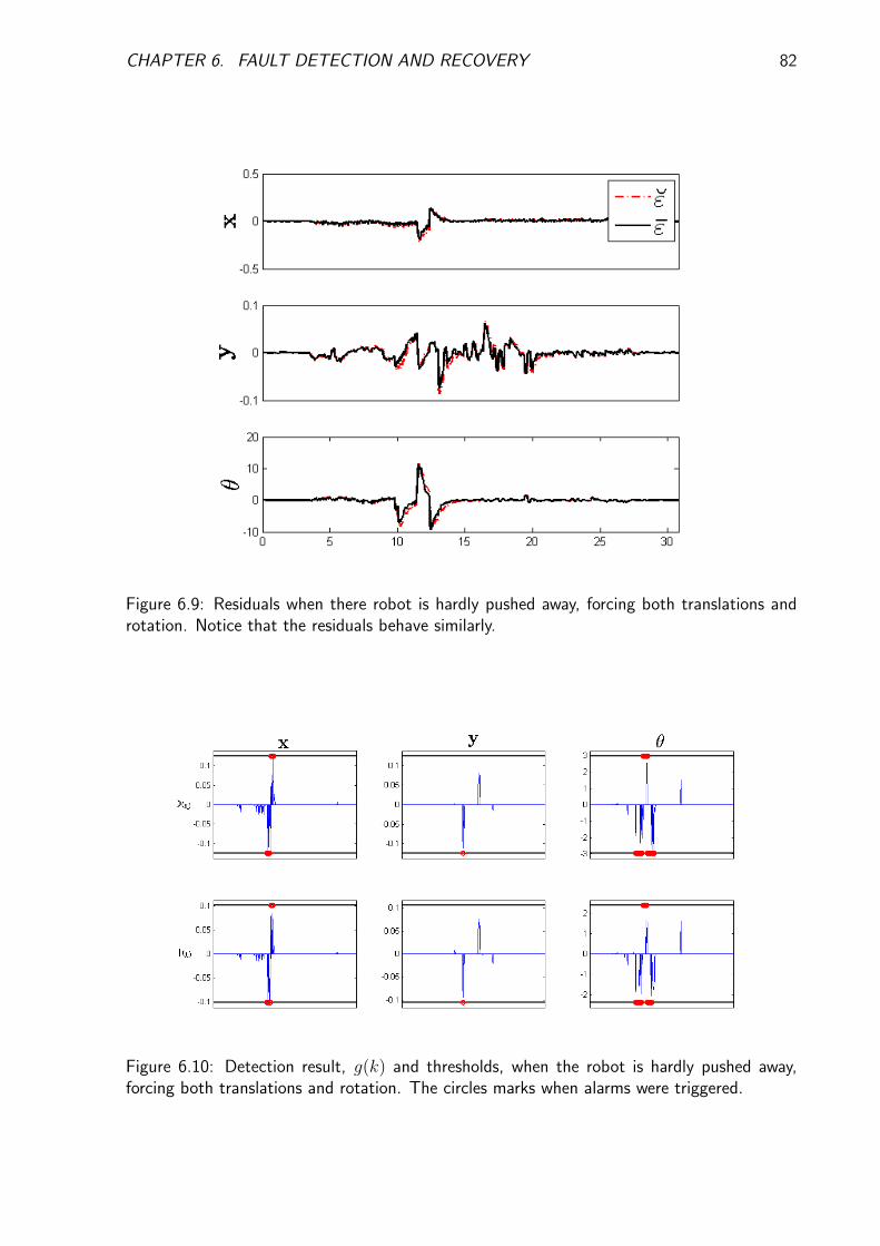
CHAPTER 6. FAULT DETECTION AND RECOVERY 82
Figure 6.9: Residuals when there robot is hardly pushed away, forcing both translations androtation. Notice that the residuals behave similarly.
Figure 6.10: Detection result, g(k) and thresholds, when the robot is hardly pushed away,forcing both translations and rotation. The circles marks when alarms were triggered.

CHAPTER 6. FAULT DETECTION AND RECOVERY 83
smaller and slower position bias than in the previous case, caused for example when
a robot is grasping an object or a wheel slippage. Experiment
The robot is held when it is moving forward, so that a fault appears in x, while
the robot is held its heading is also slightly changed, approximately, 2◦. This case is
similar to a wheel slippage, when the robot wheels rotates but no or less displacement
occurs.
Figures 6.11 and 6.12 presents the results for the residuals and detection.
Figure 6.11: Residuals when the robot is held when moving forward, simulating a wheelslippage.
6.1.4.4: Conclusions
As seem from the results, both residuals were able to detect the faults, even the
small change that occurred in the robot headings θ. It is also interesting to notice that
though y varied around ±3cm, these changes were not detected, which is due to the
fact that its normal variance as seen in Figure 6.7 are already inside this region.
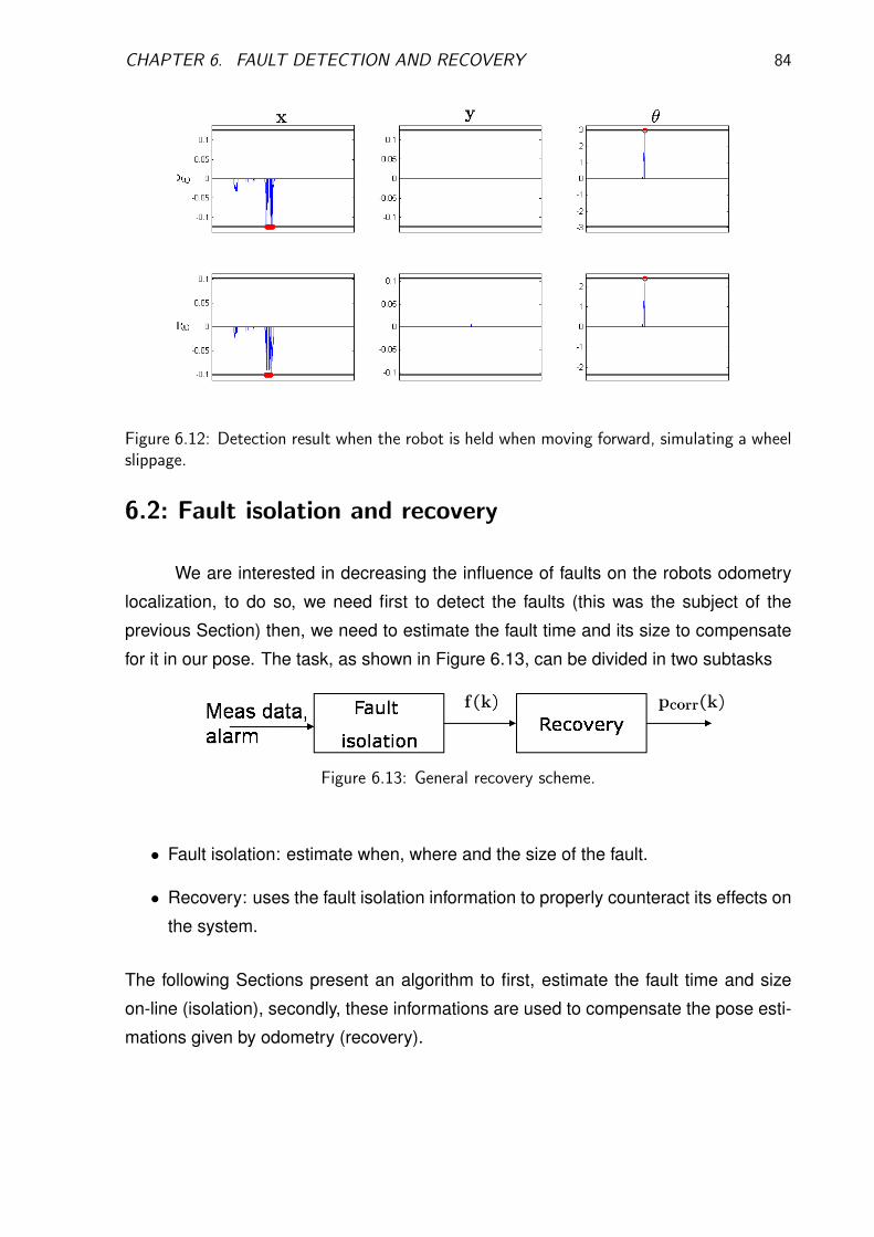
CHAPTER 6. FAULT DETECTION AND RECOVERY 84
Figure 6.12: Detection result when the robot is held when moving forward, simulating a wheelslippage.
6.2: Fault isolation and recovery
We are interested in decreasing the influence of faults on the robots odometry
localization, to do so, we need first to detect the faults (this was the subject of the
previous Section) then, we need to estimate the fault time and its size to compensate
for it in our pose. The task, as shown in Figure 6.13, can be divided in two subtasks
Figure 6.13: General recovery scheme.
• Fault isolation: estimate when, where and the size of the fault.
• Recovery: uses the fault isolation information to properly counteract its effects on
the system.
The following Sections present an algorithm to first, estimate the fault time and size
on-line (isolation), secondly, these informations are used to compensate the pose esti-
mations given by odometry (recovery).

CHAPTER 6. FAULT DETECTION AND RECOVERY 85
6.2.1: Fault isolation
As pointed earlier, we are interested in detecting and handle faults that affect our
localization system. From our change detection framework as described earlier, it is
easy to depict which direction is under the effect of a fault providing us the information
of where a fault occurred is then, easy.
A useful method to indicate the kind of a fault that occurred is the use of hy-
pothesis test and decision structure as described by Nyberg in [20]. In this approach,
several test quantities Ti (any quantity sensible to a fault) are estimated and compared
in a hypothesis test to determine which kind of fault occurred.
A hypothesis test can be defined as the decision between the two states possible
for a fault (present or not). The hypothesis test here can be seem as a matrix where
the rows represent the hypotheses and the columns the test quantities, the elements
of such matrix are the result of the test quantity for each hypothesis (each monitored
behavioral mode of the system), a 0 value means that the test quantity does not relate
to the hypothesis and an X that it can relate. The illustration presents an example where
T0 T1 T2
F1 X 0 XF2 X X 0NF 0 0 0
T0 can affect F1 and F2 and T1 can affect F2. NF stands for the non-fault hypothesis,
where none of the test quantities affect it.
In our case such Table will look like
εx εy εθ
Fx X 0 XFy 0 X XFθ 0 0 XNF 0 0 0
Table 6.1: Hypothesis test for localization faults.
where εi is the residual in the direction i and Fi is the fault in the direction i.
Notice that a fault affecting the robot headings θ can affect as well both translational
hypothesis Fx,y.
To estimate the time and size of the fault is a bit more comprehensive. We can
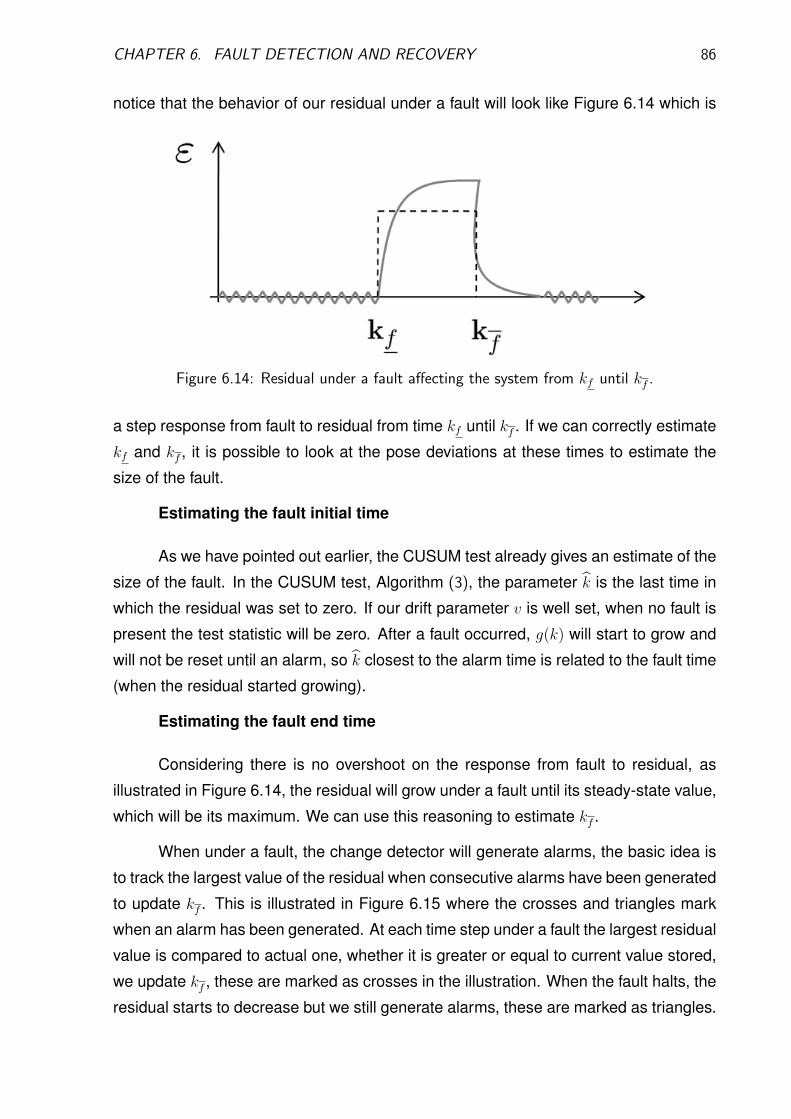
CHAPTER 6. FAULT DETECTION AND RECOVERY 86
notice that the behavior of our residual under a fault will look like Figure 6.14 which is
Figure 6.14: Residual under a fault affecting the system from kf until kf .
a step response from fault to residual from time kf until kf . If we can correctly estimate
kf and kf , it is possible to look at the pose deviations at these times to estimate the
size of the fault.
Estimating the fault initial time
As we have pointed out earlier, the CUSUM test already gives an estimate of the
size of the fault. In the CUSUM test, Algorithm (3), the parameter k is the last time in
which the residual was set to zero. If our drift parameter v is well set, when no fault is
present the test statistic will be zero. After a fault occurred, g(k) will start to grow and
will not be reset until an alarm, so k closest to the alarm time is related to the fault time
(when the residual started growing).
Estimating the fault end time
Considering there is no overshoot on the response from fault to residual, as
illustrated in Figure 6.14, the residual will grow under a fault until its steady-state value,
which will be its maximum. We can use this reasoning to estimate kf .
When under a fault, the change detector will generate alarms, the basic idea is
to track the largest value of the residual when consecutive alarms have been generated
to update kf . This is illustrated in Figure 6.15 where the crosses and triangles mark
when an alarm has been generated. At each time step under a fault the largest residual
value is compared to actual one, whether it is greater or equal to current value stored,
we update kf , these are marked as crosses in the illustration. When the fault halts, the
residual starts to decrease but we still generate alarms, these are marked as triangles.

CHAPTER 6. FAULT DETECTION AND RECOVERY 87
Figure 6.15: Residual under a fault affecting the system from kf until kf . The crossesdepict alarms with and increasing-equal residual while triangles depict alarms with a decreasingresidual.
Notice that we cannot predict when the fault will end (the actual kf ), we suppose
that, when an alarm occurred, kf is directly related to the current largest residual, at
instant k.
Estimating the fault size
Finally, we can use the information of when a fault started and when it ended
to estimate the size of the fault. Only the pose estimated from scan matching will be
sensible to the faults since the odometry estimates are based on the integration of the
wheels speeds translated to linear displacements.
We compute the size of the fault by checking the deviations of the pose in each
direction that generated an alarm from the current estimates of kf till kf . For example,
Figure 6.16 presents the x estimations of a robot pose when it is moving forward with
constant speed, in a certain moment, the robot is held, introducing a localization fault.
Every time an alarm marked as a cross (whose residual is greater than the one when
a previous alarm occurred) is generated, we look at the displacement that occurred in
the time interval from kf to ka and estimate the size of the fault, which is taken as the
difference between the scan matching pose at the time kf and ka.
Algorithm 4 presents the method for x, it should be repeated for the three param-
eters [x y θ], also notice that the CUSUM test is a one directional test, and therefore,
it should also be repeated for the other direction with CUSUM(−ε).

CHAPTER 6. FAULT DETECTION AND RECOVERY 88
Figure 6.16: Fault size estimation illustration for x. The robot starts moving forward with aconstant speed when it is held, introducing a localization fault. The fault size is estimated ateach time step according to the estimated kf and kf
Algorithm 4 Estimate fault size.Let x be the monitored parameter,
ka = −1 {alarm time initialization.}kε = −1 {time when largest residual occurred initialization.}while k do
(k, alarm) = CUSUM(εx|1:k)if alarm thenkε = max
k(‖εx(k)‖ , ‖εx(kε)× [kε > 0]‖) {get time when largest residual occurred.}
if kε == k then
kf = max(k, ka
){update fault initial time.}
ka = k {update alarm time.}∆x = x(ka)− x(kf ) {estimate fault size.}
end ifend if
end while

CHAPTER 6. FAULT DETECTION AND RECOVERY 89
6.2.2: Recovery
At last, given our detection and isolation framework, we can use the fault size
and time of occurrence to define a recovery method. The objective is to use the fault
estimate to update the odometry pose, the basic idea used here is to update the pose
using an Extended Kalman Filter. Figure 6.17 illustrates the filter inputs and outputs.
Figure 6.17: Fault recovery scheme.
Every time a fault is detected, we included its effect, ∆p(k), in the odometry pose
to update the filter output, since the measurement variances from odometry and scan
matching are different, we change also the measurement covariance matrix to consider
its different values for odometry and scan matching.
Algorithm 5 Fault recovery.
Let alarm|k be a boolean diagonal matrix with its diagonal elements relating to afault occurrence at each state at time k. And Q the process noise covariance ma-trix.
p(0) = podo(0) {set filter initial condition.}while k dop∗(k) = podo(k) + alarm|k ×∆p(k) {actual measurement with fault correction.}R = Rodo + alarm|k ×Rsm {measurement noise covariance matrix with correction.}p(k) = EKF (u(k), p(k − 1), p∗(k), Q, R)
end while
6.2.3: Case studies
Finally, with our recovery method defined, we can show some results achieved
with the recovery. We take the same cases as in Section 6.1.4 so that we can follow
with the conclusions already depicted about the detection for those cases. For sim-
plicity reasons, we will only show the result of the recovery for the residual ε(k), which
uses the augmented states observer.

CHAPTER 6. FAULT DETECTION AND RECOVERY 90
Case 1 - Normal case
There is not much to discuss when no alarm is generated since the filter will
simply track the odometry measurements so we follow and discuss the next cases.
Case 2: Hard faults
As seen in Figure 6.18, the corrected odometry pose p(k) could compensate
Figure 6.18: Residuals when there robot is hardly pushed away, forcing both translations androtation. Notice that the residuals behave similarly.
quite well the faults helping to decrease its effects on the pose. The improvements are
easily relevant to the robot headings estimate and consequently y, since rotation faults
affects it more significantly.
Case 3: Slippage faults
Our last example, shown in Figure 6.19, depicts that, again, the recovery was
successful. Even the small 2◦ fault in the robot headings was detected and handled,
improving the whole localization performance
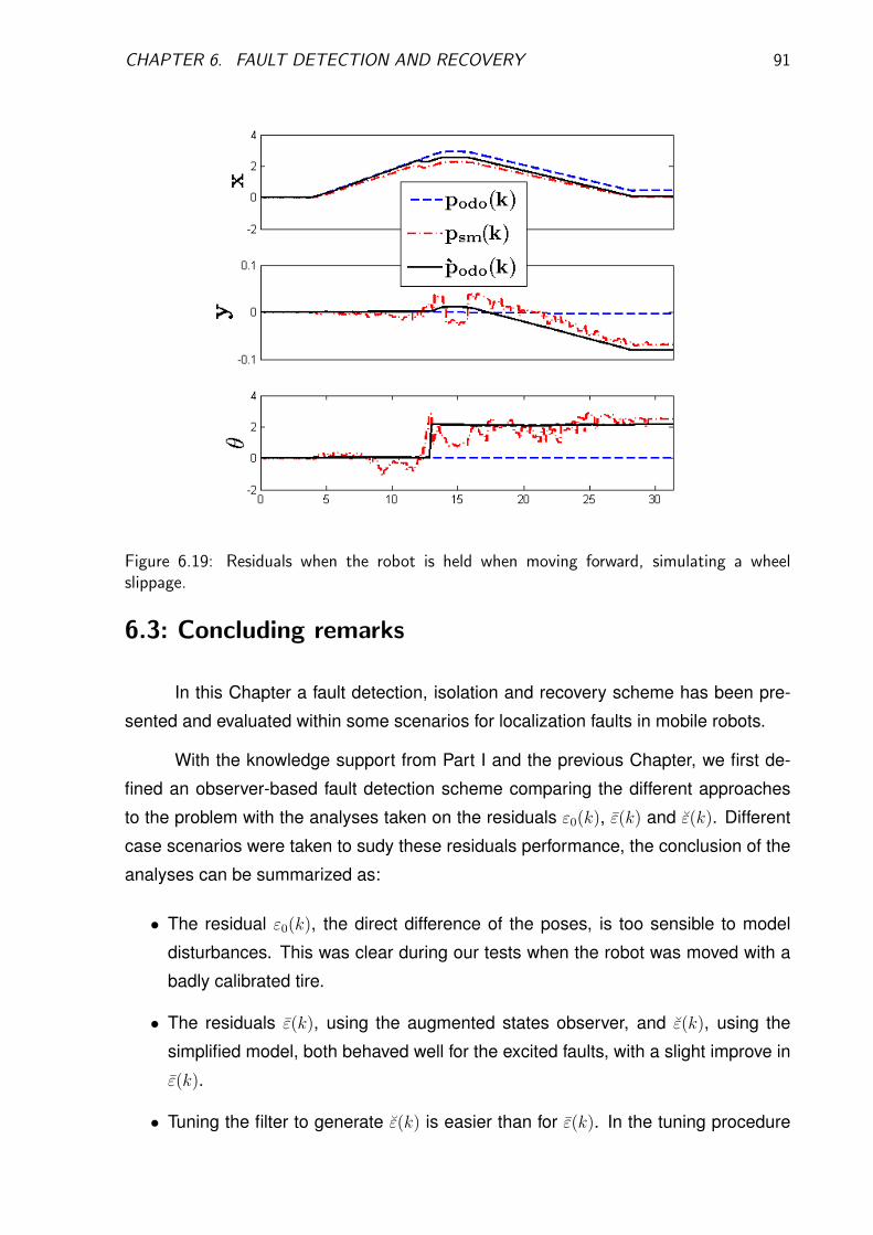
CHAPTER 6. FAULT DETECTION AND RECOVERY 91
Figure 6.19: Residuals when the robot is held when moving forward, simulating a wheelslippage.
6.3: Concluding remarks
In this Chapter a fault detection, isolation and recovery scheme has been pre-
sented and evaluated within some scenarios for localization faults in mobile robots.
With the knowledge support from Part I and the previous Chapter, we first de-
fined an observer-based fault detection scheme comparing the different approaches
to the problem with the analyses taken on the residuals ε0(k), ε(k) and ε(k). Different
case scenarios were taken to sudy these residuals performance, the conclusion of the
analyses can be summarized as:
• The residual ε0(k), the direct difference of the poses, is too sensible to model
disturbances. This was clear during our tests when the robot was moved with a
badly calibrated tire.
• The residuals ε(k), using the augmented states observer, and ε(k), using the
simplified model, both behaved well for the excited faults, with a slight improve in
ε(k).
• Tuning the filter to generate ε(k) is easier than for ε(k). In the tuning procedure

CHAPTER 6. FAULT DETECTION AND RECOVERY 92
we considered constants Q and R, process and measurement variances, this is
of course a simplification and it is expected that using more refined models for
these covariances would improve the residual performances even more.
With the definition of a fault detector, we have then presented a fault isolation and
recovery method. The detection, isolation and recovery method has been evaluated
within some case scenarios to comprove its efficacy in compensating localization faults
in the odometric pose.

7 Conclusions
This Chapter summarizes the thesis report and leave comments on future work.
7.1: Summary
The first part of this work dealt mostly with providing theoritical background/results
in fault detection, with focus to observer-integrated sensors fault detection, analyzing
several structures for observers data only fault detection.
Chapter 2 and 3 discussed standard approaches for fault detection and some
background in state observers/estimators; Chapter 4 presented ideas and addressed
some basic questions for the problem, including a discussion over fault observabil-
ity, knowledge on observer structure and residual performance measures through the
analysis of the fault sensitivity functions.
Part II, illustrated the problem through a practical example, localization fault de-
tection in mobile robots. Chapter 5 presented briefly the mobile robots field with special
attention to modeling and understanding two common localization methods in mobile
robots, odometry and laser scan matching. Chapter 6 finally accomplishes the main
objective of this works defining a localization fault detection method through integrated
sensors. It presented a framework that copes with the tasks of fault detection, isola-
tion and recovery. Such framework is relevant to the community since the localization
task is crucial for many mobile robots application, and detecting faults affecting it can
decrease its influence.
7.2: Future work
There are yet some open problems such as methods to support the choice of
the observer gains, analysis under model uncertainties, etc. We detail some of the
93

CHAPTER 7. CONCLUSIONS 94
remaining challenges:
• Analysis on the internal sensor gain knowledge L: it would be interesting to an-
alyze how uncertainties in the sensor structure, through L, affects the residual
performance in terms of detection.
• Methods to support the choice of the observer gains (tuning): the detection
method presented in Chapter 4 and 6 requires tuning which is not yet fully under-
stood and/or there is no direct method to support it that does not require some
hard constraints.
• More precise performance evaluation methods of the residuals: though we have
given some indications in Chapter 4 of which residual would perform better through
the analysis of the fault sensitivity functions they are not closed forms and more
study in this area is welcome.
• Use more refined sensor models: the covariances matrices Q and R used in the
extended Kalman filter as presented in Chapter 6 are considered constant. The
results are supposed to improve if we would consider a more complete sensor
model, using, for example a model for the error covariance in odometry and scan
matching.
• Extensive evaluation of the method: it would be interesting to check the perfor-
mance of the method presented in Chapter 6 in many cases as possible, specially
in field applications, to testify its validity as a suitable tool for system monitoring.

Bibliography
[1] P. SUNDVALL: Mobile Robot Fault Detection using Multiple Localization Modules.,
Kungliga Tekniska hogskolan, TRITA-EE 2006:044, (2007).
[2] F. GUSTAFSSON: Statistical signal processing approaches to fault detection., An-
nual Reviews in Control, 31:41–54, (2007).
[3] S. GILLIJNS AND B. DE MOOR.: Unbiased minimum-variance input and state es-
timation for linear discrete-time systems., Automatica, 43:111–116, (2007).
[4] R. ISERMANN: Supervision,fault-detection and fault-diagnosis methods - An Intro-
duction, Control Engineering Practice, 55, (1997), 639-652.
[5] R. ISERMANN: Fault-Diagnosis Systems - An Introduction from Fault Detection to
Fault Tolerance. Springer-Verlag, London, UK, 1st Edition, (2006)
[6] R. ISERMANN AND P. BALLE : Trends in the application of model-based fault de-
tection and diagnosis of technical processes, Control Engineering Practice, 55,
(1997).
[7] R. ISERMANN AND B. FREYERMUTH: Process fault diagnosis based on process
model knowledge - Part I: Principles for fault diagnosis with parameter estimation,
ASME J. of Dynamic Systems, Measurement, and Control, 113, (1991a), 620-
626.
[8] R. ISERMANN AND B. FREYERMUTH: Process fault diagnosis based on process
model knowledge - Part II: Case study, Experiments, ASME J. of Dynamic Sys-
tems, Measurement, and Control, 113, (1991a), 620-626.
[9] R. ISERMANN: Process Fault Detection Based on Modeling and Estimation
Methods-A Survey, Automatica, 204, (1984), 387-404.
[10] R. ISERMANN: Estimation of physical parameters for dynamic processes with ap-
plication to an insdustrial robot, Int J. Control, 55, (1992), 1287-1298.
95

Bibliography 96
[11] R. ISERMANN: Fault Diagnosis of machines via parameter estimation and knowl-
edge processing - Tutorial paper, Automatica, 294, (1993), 815-835.
[12] P. B. HVASS AND D. TESAR: Condition Based Maintenance for intelligent elec-
tromechanical actuators, Robotics Research Group of the University of Austin at
Texas, (2004).
[13] F. CACCAVALE: Experiments of Oberver-based Fault Detection for an Industrial
Robot, Proceedings of the 1998 IEEE International Conference on Control Appli-
cations, (1998), 480-4 vol.1.
[14] F. CACCAVALE AND ID. WALKER: Oberver-based Fault Detection for Robot Ma-
nipulators, Proceedings. 1997 IEEE International Conference on Robotics and
Automation, (1997), 2881-7 vol.4.
[15] H. SCHNEIDER AND P. M. FRANK: Oberver-based supervision and fault detection
in robots using nonlinear and fuzzy logic residual evaluation, IEEE Transactions
on Control Systems Technology, 43, (1996), 274-82.
[16] M. SAIF: Robust discrete time observer with application to fault diagnosis, IEEE
Proceedings Control Theory and Applications, 1453, (1998), 353-7.
[17] F. GUSTAFSSON: Adaptative filtering and change detection, John Wiley & Sons
Ltd., (2000).
[18] M. OSTRING: Identification, Diagnosis, and Control of a Flexible Robot Arm, Li-
centiate thesis, Linkopings universitet, Linkoping, Sweden. Linkoping Studies in
Science and Technology, (2002). Thesis No. 948.
[19] L. LJUNG AND T. SODERSTROM: Theory and practice of recursive identification,
The MIT Press, (1983).
[20] M. NYBERG: Model Based Fault Diagnosis: Methods, Theory, and Automo-
tive Engine Applications, PhD thesis, Linkopings universitet, Linkoping, Sweden.
Linkoping Studies in Science and Technology, (1999). Dissertation No. 591.
[21] P. C. YOUNG: Parameter estimation for continuous-time models - a survey, Auto-
matica, 1723, (1981).
[22] V. F. FILARETOV, M. K. VUKOBRATOVIC AND A. N. ZHIRABOK: Parity relation ap-
proach to fault diagnosis in manipulation robots, Mechatronics, 132, (2003), 141-
52.

Bibliography 97
[23] Q. WANG, Q. BI AND B. ZOU: Parameter identification of continuous-time me-
chanical systems without sensing accelerations, Computers in Industry, 82,
(1996), 207-217.
[24] E. WERNHOLT: On Multivariable and Nonlinear Identification of Industrial Robots,
Licentiate thesis, Linkopings universitet, Linkoping, Sweden. Linkoping Studies in
Science and Technology, (2004), Thesis No. 1131.
[25] L.-W. TSAI: Robot Analysis - The Mechanics of Serial and Parallel Manipulators,
John Wiley & Sons Ltd., (1999).
[26] L. LJUNG: System identification - theory for the user. Prentice Hall, Upper Saddle
River, New Jersey, USA, 2nd Edition, (1999)
[27] L.H CHIANG, E.L. RUSSELL AND R.D. BRAATZ: Fault detection and diagnosis in
industrial systems. Springer-Verlag, London, UK, 2nd Edition, (2001)
[28] A. C. BITTENCOURT: Friction change detection in industrial robots., Master Thesis
Report XR-EE-RT 026/2007, Department of Automatic Control, The Royal Insti-
tute of Technology, (2007).
[29] R. E. KALMAN: A new approach to linear filtering and prediction problems, Journal
of Basic Engineering 82 (1): 35–45, (1960)
[30] J. GERTLER: Fault detection and diagnosis in engineering systems, CRC Press,
(1998)
[31] R. ISERMANN: Model-based fault-detection and diagnosis - status and applica-
tions, Annual Reviews in Control, Volume 29, Issue 1, Pages 71-85, (2005).
[32] M. LUO, D. WANG, M. PHAM, C.B. LOW, J.B. ZHANG, D.H. ZHANG AND Y.Z.
ZHAO: Model-based fault diagnosis/prognosis for wheeled mobile robots: A re-
view, Industrial Electronics Society, IECON 2005, 31st Annual Conference of
IEEE, (2005).
[33] R. SIEGWART AND I. R. NOURBAKHSH: Introduction to autonomous mobile robots,
The MIT Press, (2004).
[34] H. B. PACEJKA : Tire and vehicle dynamics, Elsevier Science & Technology Books,
2nd Edition, (2006).

Bibliography 98
[35] J. DIXON AND O. HENLICH: Mobile robotics navigation,
http://www.doc.ic.ac.uk/~nd/surprise_97/journal/vol4/jmd/.
[36] G. ANTONELLI, S. CHIAVERINI AND G. FUSCO: A Calibration Method for Odome-
try of Mobile Robots Based on the Least-Squares Technique: Theory and Experi-
mental Validation, IEEE Transactions on Robotics, 21(5), 994–1004, (2005).
[37] A. MARTINELLI: The odometry error of a mobile robot with a synchronous
drivesystem, IEEE Transactions on Robotics, 18(3), 399–405, (2002).
[38] L. KLEEMAN: Odometry error covariance estimation for two wheel robot vehicles,
Monash University, Department of Electrical and Computer Systems Engineering,
Technical Report MECSE-95-1, (1995).
[39] S. RUSINKIEWICZ AND M. LEVOY: Efficient variants of the ICP algorithm, Proceed-
ings of the third international conference on 3-D digital imaging and modeling,
(2001).
[40] P. BESL AND N. MCKAY: A method for Registration of 3-D shapes, PIEEE Transac-
tions on Pattern Analysis and Machine Intelligence (PAMI), 14(2):239-256, (1992).
[41] E. LUNDSTROM: An analysis of scan matching methods, Master Thesis Report,
The Royal Institute of Technology, to appear.
[42] F. LU: Shape registration using optimization for mobile robot navigation, PhD The-
sis, University of Toronto, (1995).
[43] O. BENGTSSON AND A.-J. BAERVELDT: Localization in changing environments -
estimation of a covariance matrix for the IDC algorithm, Proceedings of the 2001
International Conference on Intelligent Robots and Systems, (2001).
[44] O. BENGTSSON AND A.-J. BAERVELDT: Robot localization based on scan-
matching – estimating the covariance matrix for the IDC algorithm, Robotics and
Autonomous Systems 44(1):29-40, (2003).
[45] K. KONOLIGE AND K. CHOU: Markov localization using correlation, Proceedings of
the Sixteenth International Joint Conference on Artificial Intelligence 1154–1159,
(1999).
[46] A. CENSI, L. IOCCHI, G. GRISETTI: Scan matching in the Hough do-
main, Proceedings of the IEEE International Conference on Robotics and
Automation,2739–2744, (2005).

Bibliography 99
[47] P.V.C. HOUGH: Method and means for recognizing complex patterns, U.S. Patent
3069654, (1962).
[48] R.O. DUDA AND P.E. HART: Use of the Hough transform to detect lines and curves
in pictures, Communs Ass. comput. Mach. 15, pp. 11-15., (1975).
[49] T. KAILATH: Linear systems, Prentice-Hall Prentice-Hall Information and System
Science Series, (1980).
[50] J. MESEGUER, V. PUIG, T. ESCOBET AND R. SARRATE: Observer gain effect in
linear interval observer-based fault detection, 46th IEEE Conference on Decision
and Control, 995–1002, (2007)
[51] J. CHEN AND R.J. PATTON: Robust Model-Based Fault Diagnosis for Dynamic
Systems, Kluwer Academic Publishers, (1999).
[52] D. TORQUVIST.: Statistical Fault Detection with Applications to IMU Disturbances.,
Linkoping Studies in Science and Technology, Thesis No. 1258, (2006).
[53] R. A. HORN AND C: R. JOHNSON: Matrix Analysis. Cambridge University Press,
(1985)
[54] G. F. FRANKLIN, J. D. POWELL AND A. EMAMI-NAEINI: Feedback Control of Dy-
namic Systems, Prentice Hall, Fifth edition.
[55] T. A. CHMIELEWSKI JR AND P. R. KALATA: On the Identification of Stochastic
Biases in Linear Time Invariant Systems, In Proceedings of the American Control
Conference, pages 4067-4071, Seatle, Washington, (1995).
[56] N. LIU: Optimal robust fault detection, PhD thesis,Louisiana State University,
(2008).
[57] M. ZHONG, S. X. DING, B. TANG, P. ZHANG AND T. JEINSCH: A LMI application
to robust fault detection filter design for discrete-time systems with model uncer-
tainty, Proceedings of the 40th Conference on Desision and Control, 3613-3618,
Orlando, USA, December (2001)
[58] H. B. WANG, L. LAM, S. X. DING AND M. Y. ZHONG: Iterative linear matrix in-
equality algorithms for fault detection with unknown inputs, Journal of Systems
and Control Engineering, Vol. 219, No. 2, 161-172, (2005)

Bibliography 100
[59] F. TAO AND Q. ZHAO: Fault detection observer design with unknown inputs,
Proceeding of the 2005 IEEE Conference on Control Applications, 1275-1280,
Toronto, Canada, August (2005).
[60] S. SKOGESTAD AND I. POSTLETHWAITE: Multivariable feedback control - analysis
and design, John Wiley & Sons, (1996).

ANNEX A -- Paper I
101

Observers Data Only Fault Detection ?
B. Wahlberg ∗ A. C. Bittencourt ∗∗
∗Automatic Control, KTH, SE 100 44 Stockholm, [email protected]
∗∗Automatic Control, KTH, SE 100 44 Stockholm, [email protected]
Abstract: Most fault detection algorithms are based on residuals, i.e. the difference betweena measured signal and the corresponding model based prediction. However, in many moreadvanced sensors the raw measurements are internally processed before refined informationis provided to the user. The contribution of this paper is to study the problem of fault detectionwhen only the state estimate from an observer/Kalman filter is available and not the directmeasured quantities. The idea is to look at an extended state space model where the true statesand the observer states are combined. This extended model is then used to generate residualsviewing the observer outputs as measurements. Results for fault observability of such extendedmodels are given. The approach is rather straightforward in case the internal structure of theobserver is exactly known. For the Kalman filter this corresponds to knowing the observer gain.If this is not the case certain model approximations can be done to generate a simplified modelto be used for standard fault detection. The corresponding methods are evaluated on a DCmotor example. The next step is a real data robotics demonstrator.
1. INTRODUCTION
Sensors and observers/estimators are often closely inte-grated in intelligent sensor systems. This is common indistributed sensor processing applications. It may be verydifficult or even impossible to access the raw sensor datasince the sensor and state estimator/observer often areintegrated and encapsulated. An important applicationof sensor based systems is model based fault detection,where the sensor information is used to detect abnormalbehavior. The typical approach is to study the size ofcertain residuals, that should be small in case of no fault,and large in case of faults. Most of these methods rely onthe direct sensor measurements. The problem when onlystate estimates are available is less studied. In Sundvall[2006a] and Sundvall [2006b] the problem of fault detectionfor such a system in mobile robotics is discussed frommainly an experimental point of view. The objective ofthis paper is to investigate the theoretical foundation ofobserver data only fault detection, where it is not possibleto directly access the raw measured data.
Study the system state space description
x(t+ 1) = Ax(t) +Buu(t) +Bvv(t) +Bff(t).
Here x(t) denotes the state vector, u(t) is a known inputsignal, v(t) is process disturbances and f(t) is the unknownfault input. It is common to assume that f(t) is eitherzero (no fault) or proportional to the the i:th unit vectorf(t) = fiei in case of fault number i. Hence Bf is a matrixthat determines how different faults affect the state. Thiscovers, for example, faults in actuators.
? This work was partially supported by the Swedish ResearchCouncil and the Linnaeus Center ACCESS at KTH.
The behavior of the system can be observed from differentsensors j. To simplify the analysis we assume that sensorsare integrated with standard observers/Kalman filters.
yj(t) =Cjx(t) + ej(t)
xj(t+ 1) =Axj(t) +Buu(t) +Kj (yj(t)− Cj xj(t))
The input to observer j is the measured output signal yj(t)and the input u(t). The term ej(t) represents measurementnoise. The output from the observer is xj(t), i.e., anestimate of the state. If for example the Kalman filter isused this could come with a corresponding error covariancematrix
Cov(xj(t)− x(t)) = Pj
Problem: We will study the problem when it is only pos-sible to obtain xj(t), and not the raw data yj(t). Thisseems to be a severe restriction, but from a practical pointof view the measurement process could be integrated inthe sensor system. One common example is standard GPS,where the measurement is based on satellite tracking andtriangularization based techniques. In many applicationsthe state estimate is obtained by more sophisticated meth-ods then a simple linear observer. We will however usethis structure for analysis and design purposes, so that theproblem can be approached through well studied/standardFDI techniques.
Sofar we have not taken the fault contribution f(t) intoaccount. One possibility is to also estimate f(t) by forexample extending the state vector to x(t) = [x(t) f(t)]Tand apply the Kalman filter or another observer methodto estimate the extended state vector x(t). Recently, therehas been quite a lot of progress in the area of inputestimation using Kalman filtering, see Gillijns et al. [2007].

2. RESIDUAL BASED FAULT DETECTION
There are in principle two paradigms for residual basedfault detection. We will start with the standard problemformulation, with a direct measurable output.
x(t+ 1) =Ax(t) +Buu(t) +Bvv(t) +Bff(t)
y(t) =Cx(t) + e(t) +Dff(t) (1)Here we also have the possibility to model and detectsensor faults via Df . The dimension of x(t) is nx and thedimension of y(t) is ny.
The so-called parity space approach, recently reviewed inGustafsson [2007], is based on a sliding window formula-tion of the state space equationsY (t) = Ox(t−L+ 1) +HuU(t) +HvV (t) +HfF (t) +E(t)
where Y (t) =[yT (t− L+ 1) . . . yT (t)
]T and similar forthe other signal vectors. The matrices are given by
O =
CCA
...CAL−1
, Hf =
Df 0 . . . 0CBf Df . . . 0
.... . .
...CAL−2Bf . . . CBf Df
and Hv and Hu are constructed in the same way as Hf ,i.e. from the corresponding impulse response coefficients.The residual is then defined by
R(t) = WT (Y (t)−HuU(t))where W is an L×nr projection matrix such that WTO =0. The dimension nr = Lny − nx, where ny is thedimension of the output vector y(t) and nx is the statedimension. This still leaves freedom in the choice of W ,which can be used to obtain more structured residuals. InGustafsson [2007] gives detailed insights of the design andanalysis of parity space based methods in case of stochasticdisturbances and noise.
An alternative approach is to use an observer or a Kalmanfilter to estimate x(t) and then study the size of theresiduals
R(t) = (Y (t)−Ox(t− L+ 1)−HuU(t))The choice L = 1 just gives the standard innovationprocess r(t) = y(t) − Cx(t) used in the observer and inthe Kalman filter to update the state estimate.
It is most important that the effects of the faults arevisible in the residual vector. A fault is detectable ifthe transfer function from fault to residual is non-zero,this condition holds even for faults that disappear in theresidual after some transient and a stronger condition isthat this transfer function is non-zero also in steady-state.Another way to check if certain faults are detectable isto calculate if the extended state space model x(t) =[x(t) f(t)]T is observable in classical state space sense.It is also closely related to input estimation, for whichconditions are given in Gillijns et al. [2007].
It is also desirable different faults to be distinguishablebetween each other through the residual. A classical ap-proach is to define structured residual sets that are sen-sitive to one fault and whilst remaining unsensitive toothers. An alternative is to design a directional residual
vector; with each fault corresponding to a direction, iso-lation is achieved by deciding which direction the gener-ated residual is closest to. The diagnosticability matrix aspresented in Gustafsson [2007], is an off-line method toevaluate the isolation in a directional residual set, givingthe probabilities of generating alarms for fault i given faultj occurred and also in case there is no fault.
3. RESIDUAL BASED FAULT DETECTION USINGOBSERVER DATA ONLY
Residual based techniques are all based on comparinga predicted output yj(t), based on a model, with theobserved output yj(t) from a sensor. In case of a systematicdifference we will alarm. If only the observer states xj(t)are available the first two ideas for fault detection ideaswould be:
• Try to reconstruct yj(t) using a model of the observer,e.g.Kjyj(t) = xj(t+ 1)− (A−KjCj)xj(t)−Buu(t)
Here we need a very accurate model and the internalstructure of the observer, e.g. the gain Kj , otherwisethe estimations will be easily biased. In many prac-tical cases this would be difficult. Notice also that ifKj is not full rank, it allows for multiple solutions.
• Assume that there are at least two observers provid-ing x1(t) and x2(t). Define the residual vector
ε(t) = x1(t)− x2(t)which should be sensible to fault that affects thetwo observers in different ways, e.g. sensor faults.This approach does not, however, make direct use ofthe model of the system and requires at least oneredundant sensor.
We will start by analyzing the case with only one observer.
Idea: View x(t) as the output from the extended system
x(t+ 1) =Ax(t) +Buu(t) +Bff(t)
x(t+ 1) =Ax(t) +Buu(t)
+K (Cx(t) +Dff(t)− Cx(t))
y(t) =C∗x(t) (2)where C∗ depicts which estimates are available. By usingthe extended state x(t) = [xT (t) xT (t)]T and the corre-sponding state space matrices we can interpret this a stan-dard fault detection problem, which could be approachedby a parity space method or a Kalman filter based method.The problem when we have m different observers canbe approached by augmenting the state space with allobserver states xj(t), j = 1, . . .m.
There are some basic questions that need to be addressed
• Are the faults detectable using this model?• What to do if the observer gain K is unknown?• How to compare/validate the performance of different
methods?
3.1 Fault Observability
As described in Kalata et al. [1995], stochastic biasesin linear time invariant systems can be identified by

augmenting the system state with a bias and implementa Kalman filter. The author utilizes this technique toidentify biases in noisy measurements. In Chapter 3 inTornqvist [2006] these results are extended to check theobservability of additive faults with the constrain thatf(t + 1) = f(t). An important characteristic explored byboth authors is the observability issue.
Considering a system as in Equation (2), where only esti-mated states x(t) are available but not x(t), we can aug-ment the faults in the states as x(t) = [x(t) x(t) f(t)]and analyze the observability with the pair
C = [ 0 C∗ 0 ] , A =
[A 0 BfKC (A−KC) KDf
0 0 I
](3)
Observability conditions: With a similar approach asin Tornqvist [2006] Appendix A shows that if the originalsystem is observable (pair (A,C) observable) and if
• All state estimates are directly available at the output(i.e. C∗ = I).• K is full column rank, such that
Kz = 0 ⇒ z = 0
then the extended system will be observable under thesame conditions for sensor and process faults as when theactual output y(t) is available. In other words, we will havethe same information as when y(t) is directly accessible.The conditions can be summarized as:
• For measurement faults only, if the system has nointegrator dynamics (modes with eigenvalue equals to1), the faults will be observable as long as Df is fullrank. If there is an integrator, then the faults are notobservable if Df is full rank and the states throughwhich the fault propagates should be orthogonal tothe measured integrating part of the system.• For process faults only, the faults should be orthog-
onal to the contribution of the non-measured part ofthe system.
3.2 Unknown Observer Structure
If the observer structure is not given, for example if K isunknown, we cannot directly use the extended state spacemodel for fault detection. To overcome this problem, let usmake two approximations. The first one is to approximate
K (Cxf (t) +Dff(t)) ≈ Ff f(t)Here
xf (t+ 1) = Axf (t) +Bff(t) (4)
and xf (t) is the fault contribution in x(t). Since f(t) iszero or a constant vector it is most important that thisapproximation holds stationary i.e. after transients.
The second approximation isK (y(t)− Cx(t)) ≈ v(t)
where v(t) is a white noise process with a certain covari-ance matrix. This makes sense from a Kalman filter pointof view where the innovations can be viewed as processnoise, v(t) = Kε(t) where ε(t) = y(t) − Cx(t) is a whiteinnovation process.
This leads to the simplified model
x(t+ 1) =Ax(t) +Buu(t) + Ff f(t) + v(t)
y(t) = x(t) + e(t) (5)With such structure, actuator and sensor faults are mixedand the fault isolation step could be more difficult in thissetting.
The artificial measurement noise e(t) can be used tocope with unmodeled characteristics of the system. Forexample, for sensors over a network or with a weak real-time performance, one can use e(t) to include jitter,missed samples, delays, etc. or to cope with sensor/systemunknown dynamics.
After defining e(t), it can be used to tune a Kalman filterobserver for the system as in Equation (5) and a standardparity space method or Kalman filter based method canbe used to design a fault detection algorithm. It is easyto extend this approach to several observers by combiningthe observer states as
x1(t+ 1)x2(t+ 1)
...xj(t+ 1)
= A
x1(t)x2(t)
...xj(t)
+ Buu(t) + Ff f(t) + v(t)
where A, Ff and Bu are diagonal matrices relatingobservers and fault states and actuator dynamics, andu(t),f(t) and v(t) are the extended control, fault and noiseinputs.
3.3 Performance evaluation methods
We are interested in analyzing the quality of the residu-als generated by the different methods rather than for afull detection scheme. Different factors influence a resid-ual success in terms of detection, including noise/modeldisturbances decoupling and sensitivity to faults. Thesequalities are often in contradiction and can be seem asan optimization problem. Some recent results for optimalresidual generation can be found in Liu [2008], where theauthor shows closed-form solutions for some sets of theproblem, the solutions however, require that the faultsare directly visible at the output (full column rank Df ),which will never be the case for sensors integrated withobserver/Kalman filters since the faults travel through theobserver dynamics before they appear in the output.
For the analysis of our proposed methods, we will usea definition of a good residual as one that resembles towhite gaussian noise with no peaks or abrupt changes in afault-free case (possibly decreasing the false-alarm rates)and that bias under a fault as great as possible (possiblyincreasing the detection rate). We depict two empiricalquantities to relate these qualities.
The kurtosis statistic is a measure of the peakedness ofa signal, we can use it to analyze the resemblance of theresiduals over a fault-free scenario (NF ) to a gaussiandistribution. It is defined as
κ =E[ε(t)|NF − µε(t)|NF
]4
σ4ε(t)|NF
− 3
where µε(t)|NFand σε(t)|NF
are the mean and standarddeviation of the residual under no-fault while E[z] is

the expected value of z. For a gaussian residual the testapproximates to zero, and it is usually used to detectabrupt variations over a gaussian signal. In Hadjileontiadiset al. [2005], for instance, it is used for crack detectionover a beam with vibration analysis. Basically, a κ closeto 0 will relate to a white gaussian distribution whilehigher κ means more of the variance is due to big sporadicdeviations or biases.
The fault-to-noise ratio as defined in Gustafsson [2001] isa measure of a fault sensitivity relative to noise and isdefined as a ratio between the expected value of a faultinfluence in the system output and the noise variance, itis, in fact, a similar concept as the signal-to-noise-ratio(SNR) but applied to a fault. For a known FNR, we candefine the measure
δ =∣∣∣∣[ε(t)|F ]/σε(t)|F
FNR
∣∣∣∣where E[ε(t)|F ] and σε(t)|F are the expected value andstandard deviation of the residual under a fault hypothesis(F ). In this manner, δ will vary from 0 to 1 (best possibleresidual, which will have the same quality as the directfault influence to the output, only possible if we use a per-fect simulator of the system to generate the redundancy).
4. ILLUSTRATIVE EXAMPLE
In order to explore the different configurations presented,we consider a simple linear DC motor, as shown in Figure1. Non-linearities such as flexibilities and friction aresimplified. The applied voltage in the motor terminals isthe controlled input to the system Vapp while angular speedis taken as output. The states are current and angular
Fig. 1. DC motor model.
speed x(t) = [i(t) ω(t)]T and the governing matrices
A =
−RL−kbL
kmJ
−kfJ
, B =
[1L
0]T
C = [ 0 1 ] , D = [ 0 ]
(6)
where km, kb and kf are armature, emf and frictionconstants. Process noise with variance Q, is considered toaffect the system as random oscillations in the current i(t).While measurement noise with variance R, appears in theangular speed measurements. So that Bw = [ 1 0 ]T andDv = [1].
Integrated sensor model. We are interested in study-ing the residuals when only the state estimate from anobserver/Kalman filter is available and not the directmeasured quantity. For this purpose we use a sensor model
integrated with an observer as in Equation (2). TakingC∗ = C and the observer gain K as the stationary Kalmanfilter gain for the given process and noise covariances, Qand R. During our example, this model should be referredto whenever we use the notation y(t).
Faults. Two step faults with FNR = 10 (that produces a10 times greater amplitude in the sensor output y(t) thanthe present noise) are considered: process faults, fp(t),appearing as a step torque opposing to the system; sensorfaults, fs(t), an offset measurement deviation. So that
Bf =[
0 − 1J
]Tand Df = [1].
In the following Sections we discuss the performance ofdifferent methods to generate the residual considering theoutput of such integrated sensors.
4.1 Augmented system observer
When K is known, a possible approach to generate aresidual is to augment system and sensor states x(t) =[x(t) x(t)] and use the augmented model
A =[A 0KC (A−KC)
], Bu =
[BuBu
], C =
[0C
]T
to design an observer/Kalman filter. With the redundantoutput y(t) from this model we can set a residual as ε(t) =y(t) − y(t) to detect faults. Considering our DC motorexample, when we configure our observer as a Kalmanfilter with gain L, we have for process and sensor faultsa response as shown in Figure 2 from which is easy to
Fig. 2. Residual y(t) for process and sensor fault (solid line)together with direct fault contribution to the sensoroutput yf (t).
depict that the residual performance is good. In fact, forprocess faults we had (δ, κ) = (0.88, ≈ 0) and sensorfaults (0.85, ≈ 0).
Is is important to analyze how robust this method is tomodel errors introduced through errors in the sensor gainK. We analyze the sensitivity of the residual to K byvarying it with a scaling factor as K × α while L remainsconstant. The pair (δ, κ) is computed for α varying within[10−1, 105]. The result is a pair (δ, κ) = (0.85, 0.30) inthe worst case showing the robustness of the approach inthis example.

4.2 Simplified system observer
As discussed in Section 3.2, we can simplify the sensordynamics yielding a model as in Equation (5), with faultsand internal observer dynamics appearing in the termsFf f(t) and v(t). With this simplification, we can designan observer to generate a redundancy y(t) and a residualε(t) = y(t)− y(t) sensible to faults.
In our example, we set the observer gain equal to the sensorgain, L = K. In this setting, the observer has similardynamics to the sensor, in fact, if we could use the directmeasured output y(t) as input to our observer, sensor andobserver would be equivalent. For a process fault, we have(δ, κ) = (0.87, ≈ 0) and sensor fault (0.84, ≈ 0) which isa slightly worsened result when compared to the results inthe earlier Section, with the augmented system observer.
To analyze the robustness on the gain selection, L, weagain, vary it with a scaling factor as L = K ×α and plotthe pair (δ, κ). The result, shown in Figure 3, indicates
Fig. 3. δ and κ versus scaling factor α for process andsensor faults. The circle depicts the case when L = K.
that the residual is worsened with the overestimation of K.This result is to be expected since, the larger the gain, themore relevance is given to the measurements and therefore,the residual will be less sensitive to faults (δ decrease).As well, it also increases the observer speed, with theobserver trying to reach the signal faster and consequentlyincreasing transient errors (κ increase).
4.3 Multiple sensors
A common approach to fault detection is to take a residualas the direct difference between two redundant sensorsε(t) = yi(t) − yj(t). We study this case for our examplecomparing its performance with model-based generatedresiduals.
So far, our sensor estimates the states through angularspeed measurements, yω(t). To provide a redundancy, wedepict a sensor that estimates the states through positionmeasurements θ(t), yθ(t). Notice that the subscript inyθ(t) and yω(t) denotes directly what is the measuredquantity. For such redundant sensor, we have the states[i(t) ω(t) θ(t)] and model,
A =
−RL−kbL
0kmJ
−kfJ
00 1 0
, B =
1L00
, C =
[ 001
]T(7)
we suppose this sensor is also integrated with a Kalmanfilter and outputs an estimate of ω(t). The sensor noisevariance is set to produce the same error order in theoutput as for the first sensor so that both have similarqualities. We would like to compare the classical approach,ε0(t) = yω(t) − yθ(t), with model based generated resid-uals. We consider one augmented states observer for eachavailable sensor, yω(t) and yθ(t) with the residuals as
εω(t) = yω(t)− yω(t)
εθ(t) = yθ(t)− yθ(t)εω, θ(t) = yω(t)− yθ(t) (8)
Because the sensors are different, the same fault maycause different influences in the output for each sensor, butsince we are interested in showing the relative performancebetween model-based generated residuals and ε0(t), wecompute a relative measure as
∆ =∣∣∣∣E[εi(t)|F ]/σεi(t)|FE[ε0(t)|F ]/σε0(t)|F
∣∣∣∣where εi(t) is one of the residuals from Equation 8. ∆ >1 will depict a residual with a larger fault sensitivitythan the one generated by ε0(t). Table 1 shows ∆ forprocess and sensor faults. The results show that taking
Residual ∆ for process fault ∆ for sensor yω(t) fault
εω(t) 0.1498 1.6059εθ(t) 1.3890 ≈ 0.00
εω, θ(t) 3.0104 0.02
Table 1. ∆ for different faults. In all casesκ ≈ 0.
the residual as the direct difference between sensors, ε0(t),may not provide the best residual. It is expected thiswould be even more significant in case the noise variancesdiffered considerably for each sensor, since the observersalso attenuate noise.
4.4 Example summary
Different aspects have been analyzed trough our illustra-tive examples, some important remarks:
• Though this was not fully explored in the example,different tuning configurations have been used andit was noticed that the use of an augmented statesobserver is likely to improve the fault sensitivity whencompared to the observer using a simplified sensormodel as presented in Section 4.2.
• The analysis on the observer gain choice in Section4.2 indicates that the fault sensitivity is improved assmaller we choose the gain. Such result is motivatedby the fact that lower gains will thrust more on themodel and therefore, the resulting residual will bemore sensitive to unmodeled influences, such as faults.Nevertheless, the choice of the gain should actually beseem as a compromise between model uncertaintiesand the fault sensitivity.
• Finally, the example with multiple sensors depictedthat using a model-based residual can improve thefault sensitivity.
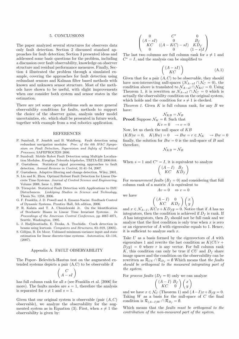
5. CONCLUSIONS
The paper analyzed several structures for observers dataonly fault detection. Section 2 discussed standard ap-proaches for fault detection; Section 3 presented ideas andaddressed some basic questions for the problem, includinga discussion over fault observability, knowledge on observerstructure and residual performance measures. Finally, Sec-tion 4 illustrated the problem through a simulated ex-ample, covering the approaches for fault detection usingredundant sensors and Kalman filter based methods withknown and unknown sensor structure. Most of the meth-ods have shown to be useful, with slight improvementswhen one consider both system and sensor states in theestimation.
There are yet some open problems such as more generalobservability conditions for faults, methods to supportthe choice of the observer gains, analysis under modeluncertainties, etc. which shall be presented in future work,together with example from a real robotics application.
REFERENCES
P. Sundvall, P. Jensfelt and B. Wahlberg. Fault detection usingredundant navigation modules. Proc. of the 6th IFAC Sympo-sium on Fault Detection, Supervision and Safety of TechnicalProcesses, SAFEPROCESS 2006.
P. Sundvall. Mobile Robot Fault Detection using Multiple Localiza-tion Modules. Kungliga Tekniska hogskolan, TRITA-EE 2006:044.
F. Gustafsson. Statistical signal processing approaches to faultdetection. Annual Reviews in Control, 31:41–54, 2007.
F. Gustafsson. Adaptive filtering and change detection. Wiley, 2001.N. Liu and K. Zhou. Optimal Robust Fault Detection for Linear Dis-
crete Time Systems. Journal of Control Science and Engineering,Volume 2008, Issue 1, 2008.
D. Tornqvist. Statistical Fault Detection with Applications to IMUDisturbances. Linkoping Studies in Science and Technology,Thesis No. 1258, 2006.
G. F. Franklin, J. D. Powell and A. Emami-Naeini. Feedback Controlof Dynamic Systems. Prentice Hall, 5th edition, 2006.
P. R. Kalata and T. A. Chmielewski Jr. On the Identificationof Stochastic Biases in Linear Time Invariant Systems. InProceedings of the American Control Conference, pp 4067-4071,Seattle, Washington, 1995.
L. J. Hadjileontiadis, E. Douka, A. Trochidis. Crack detection inbeams using kurtosis. Computers and Structures, 83:-919, (2005).
S. Gillijns, B. De Moor. Unbiased minimum-variance input and stateestimation for linear discrete-time systems. Automatica, 43:-116,(2007).
Appendix A. FAULT OBSERVABILITY
The Popov- Belevitch-Hautus test on the augmented ex-tended systems depicts a pair (A,C) to be observable if(
CA− sI
)
has full column rank for all s (see Franklin et al. [2006] formore). The faults modes are s = 1, therefore the analysisis separated for s 6= 1 and s = 1.
Given that our original system is observable (pair (A,C)observable), we analyze the observability for the aug-mented system as in Equation (3). First, when s 6= 1 theobservability is given by:
0 C∗ 0(A− sI) 0 BfKC ((A−KC)− sI) KDf
0 0 (1− s)I
The last two columns are full column rank for s 6= 1 andC∗ = I, and the analysis can be simplified to
((A− sI)KC
)(A.1)
Given that for a pair (A,C) to be observable, they shouldhave non-intersecting null-spaces (NA−sI ∩ NC = 0), thecondition above is translated to NA−sI ∩NKC = 0. UsingTheorem 1, it is rewritten as NA−sI ∩ NC = 0 which isactually the observability condition on the original system,which holds and the condition for s 6= 1 is checked.Theorem 1. Given K is full column rank, for any B wehave:
NKB = NBProof: Suppose NK = ∅. Such that
Kv = 0 → v = 0Now, let us check the null space of KB(KB)w = 0, K(Bw) = 0 → Bw = r ∈ NK → Bw = 0finally, the solution for Bw = 0 is the null-space of B andtherefore,
NKB = NB
When s = 1 and C∗ = I, it is equivalent to analyze((A− I) BfKC KDf
)
For measurement faults (Bf = 0) and considering that fullcolumn rank of a matrix A is equivalent to
Av = 0 ⇔ v = 0we have (
(A− I) 0KC KDf
)(xy
)
and x ∈ NA−I , KCx+KDfy = 0. Notice that if A has nointegrators, then the condition is achieved if Df is rank. IfA has integrators, then Df should not be full rank and weanalyze that the first condition is only true when x is zeroor an eigenvector of A with eigenvalue equals to 1. Hence,it is sufficient to analyze such x.
Take U as a basis formed by the eigenvectors of A witheigenvalues 1 and rewrite the last condition as K(CUr +Dfy) = 0 where r is any vector. For full column rankK, this condition can only be true if CU and Df shareimage spaces and the condition on the observability can berewritten as RCU ∩RDf
= ∅ Which means that the faultsshould be orthogonal to the measured integrating part ofthe system.
For process faults (Df = 0) only we can analyze((A− I) BfKC 0
)(xy
)
and we have x ∈ NC (Theorem 1) and (A−I)x+Bfy = 0.Taking W as a basis for the null-space of C the finalcondition is R(A−I)W ∩RBf
= ∅.Which means that the faults must be orthogonal to thecontribution of the non-measured part of the system.