Fatigue of Stabilized SS and 316 NG Alloy in PWR Environment

Downl

Proceedings of PVP 2006-ICPVT11 2006 ASME Pressure Vessel and Piping Division Conference

July 23-27, 2006, Vancouver, BC, Canada

PVP2006-ICPVT11-93833

FATIGUE OF STABILIZED SS AND 316 NG ALLOY IN PWR ENVIRONMENT

Jussi P. Solin VTT Technical Research Centre of Finland

Kemistintie 3, Espoo FI-02044 VTT, Finland

[email protected]

Proceedings of PVP2006-ICPVT-11 2006 ASME Pressure Vessels and Piping Division Conference

July 23-27, 2006, Vancoucer, BC, Canada

PVP2006-ICPVT-11-93833

ABSTRACT Strain controlled constant and variable amplitude fatigue

tests for 316 NG and Titanium stabilized stainless steels in low oxygen PWR waters were performed. The stabilized steel has been plant aged for 100 000 hours.

Constant amplitude test results at 0,01 Hz sinusoidal straining comply with predicted lives according to the Fen approach for both materials. Spectrum straining both in air and in environment caused predicted life reduction factors (about 3) for the stabilized steel, but for the 316 NG steel spectrum straining in environment resulted to a larger reduction in life.

NOMENCLATURE εa ; εa,i strain amplitude [at a level (i) in spectrum] ε' strain rate (for sinusoidal ramps ε' = 2⋅∆ε / f ) εa,eq equivalent (constant) strain amplitude f frequency Fen = Fen, nom reduction of life due to environment F(spectrum) reduction of life due to spectrum straining Di ; ni damage and cycles at a level (i) in spectrum Neq equivalent number of cycles (with εa,eq) Nf,25 fatigue life (cycles) at 25% peak load drop Nf(RT,air) fatigue life in room temperature air Nf,(T,environment) fatigue life in environment and temperature DO Dissolved oxygen content in water T ; RT Temperature, room temperature T* ; O* ; ε'* transformed T, DO and ε'

INTRODUCTION Fatigue design curves given in the ASME Code Section III

are based on strain controlled low cycle fatigue tests in room temperature. Protection against environmental effects was left as a responsibility of the designer.

oaded From: https://proceedings.asmedigitalcollection.asme.org on 06/29/2019 Terms of U

Later on, extensive studies were launched in USA and in Japan to quantify environmental effects on fatigue life. The research in Argonne National Laboratory resulted to statistical models for estimating the fatigue lives in air and LWR environments (1). An alternative approach for presenting the environmental effects in terms of an environmental fatigue correction factor Fen was proposed by Higuchi and Iida (2). Mehta used the ANL statistical models for calculating Fen in an approach known as the EPRI/GE methodology (3,4). To account for the latest data Chopra and Higuchi have occa-sionally updated the expressions to calculate Fen (5-7).

Rather general consensus exists on the models and main parameters applicable to present laboratory data on small specimens. But significance of the laboratory data to component behavior in real plants is still an issue for debate.

Codes and guidelines Environmental effects have been discussed in terms of

proposed fatigue curve revisions to account for the newest experimental data, but common agreement for such revisions is lacking. Meanwhile, environmental effects and Fen models have already been adopted for in license renewals in USA and for plant life management in Japan. The Japanese utilities were notified in 2000 to adopt MITI guidelines for evaluating fatigue initiation life reduction in LWR environments and a revised approach was published in 2002 as TENPES Guidelines (8,9).

The EPRI/GE methodology has been applied for license renewals in USA and it has been reviewed by the Pressure Vessel Research Council (PVRC/CLEE (4). In 2004 this methodology was introduced in the ASME Code as follows: “proposed in the form of a nonmandatory Appendix … and may possibly be considered for Code implementation” (10).

Status in Finland Since 2002 consideration of fatigue damage rate in high

temperature water environment has been mandatory for new

1 Copyright © 2006 by ASME

se: http://www.asme.org/about-asme/terms-of-use

designs in Finland (11). Steps have been taken in aim to adopt related measures also in plant life management of the running plants. Two BWR and two VVER plants are currently running in Finland, and one PWR is under design and construction.

To be able to measure specific environmental effects, novel experimental capabilities have been developed by VTT. A modest testing activity is running as part of a national research program. This paper reports the progress in the VTT experiments. As results for alloy 316 NG have been presented earlier (12), this paper concentrates mainly on new results for plant aged Titanium stabilized stainless steel. However, alloy 316 NG data is partially repeated for comparison.

EXPERIMENTAL Fatigue testing equipment

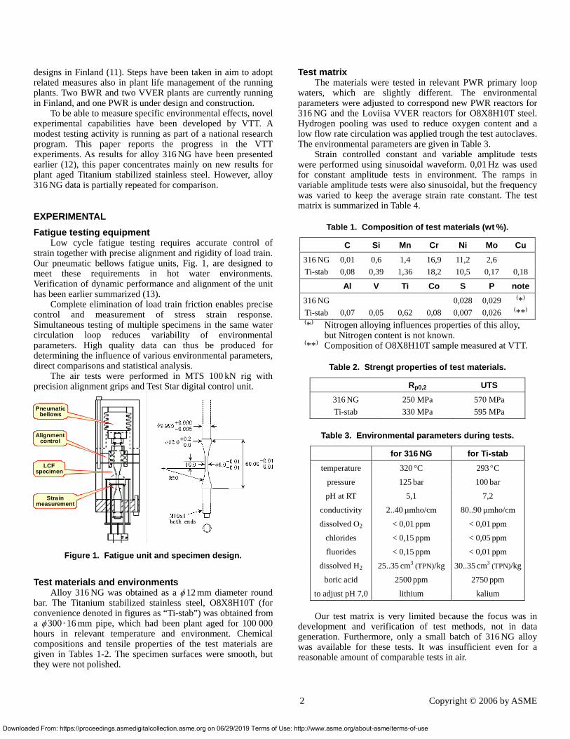
Low cycle fatigue testing requires accurate control of strain together with precise alignment and rigidity of load train. Our pneumatic bellows fatigue units, Fig. 1, are designed to meet these requirements in hot water environments. Verification of dynamic performance and alignment of the unit has been earlier summarized (13).

Complete elimination of load train friction enables precise control and measurement of stress strain response. Simultaneous testing of multiple specimens in the same water circulation loop reduces variability of environmental parameters. High quality data can thus be produced for determining the influence of various environmental parameters, direct comparisons and statistical analysis.

The air tests were performed in MTS 100 kN rig with precision alignment grips and Test Star digital control unit.

Pneumaticbellows

Strainmeasurement

Alignmentcontrol

LCFspecimen

Pneumaticbellows

Strainmeasurement

Alignmentcontrol

LCFspecimen

Pneumaticbellows

Strainmeasurement

Alignmentcontrol

LCFspecimen

Figure 1. Fatigue unit and specimen design.

Test materials and environments Alloy 316 NG was obtained as a φ 12 mm diameter round

bar. The Titanium stabilized stainless steel, O8X8H10T (for convenience denoted in figures as “Ti-stab”) was obtained from a φ 300 x 16 mm pipe, which had been plant aged for 100 000 hours in relevant temperature and environment. Chemical compositions and tensile properties of the test materials are given in Tables 1-2. The specimen surfaces were smooth, but they were not polished.

Downloaded From: https://proceedings.asmedigitalcollection.asme.org on 06/29/2019 Terms of Us

Test matrix The materials were tested in relevant PWR primary loop

waters, which are slightly different. The environmental parameters were adjusted to correspond new PWR reactors for 316 NG and the Loviisa VVER reactors for O8X8H10T steel. Hydrogen pooling was used to reduce oxygen content and a low flow rate circulation was applied trough the test autoclaves. The environmental parameters are given in Table 3.

Strain controlled constant and variable amplitude tests were performed using sinusoidal waveform. 0,01 Hz was used for constant amplitude tests in environment. The ramps in variable amplitude tests were also sinusoidal, but the frequency was varied to keep the average strain rate constant. The test matrix is summarized in Table 4.

Table 1. Composition of test materials (wt %).

C Si Mn Cr Ni Mo Cu 316 NG 0,01 0,6 1,4 16,9 11,2 2,6 Ti-stab 0,08 0,39 1,36 18,2 10,5 0,17 0,18

Al V Ti Co S P note 316 NG 0,028 0,029 (*) Ti-stab 0,07 0,05 0,62 0,08 0,007 0,026 (**) (*) Nitrogen alloying influences properties of this alloy,

but Nitrogen content is not known. (**) Composition of O8X8H10T sample measured at VTT.

Table 2. Strengt properties of test materials.

Rp0,2 UTS 316 NG 250 MPa 570 MPa Ti-stab 330 MPa 595 MPa

Table 3. Environmental parameters during tests.

for 316 NG for Ti-stab temperature 320 °C 293 °C

pressure 125 bar 100 bar

pH at RT 5,1 7,2

conductivity 2..40 µmho/cm 80..90 µmho/cm

dissolved O2 < 0,01 ppm < 0,01 ppm

chlorides < 0,15 ppm < 0,05 ppm

fluorides < 0,15 ppm < 0,01 ppm

dissolved H2 25..35 cm3 (TPN)/kg 30..35 cm3 (TPN)/kg

boric acid 2500 ppm 2750 ppm

to adjust pH 7,0 lithium kalium Our test matrix is very limited because the focus was in

development and verification of test methods, not in data generation. Furthermore, only a small batch of 316 NG alloy was available for these tests. It was insufficient even for a reasonable amount of comparable tests in air.


e: http://www.asme.org/about-asme/terms-of-use

Down

Table 4. Summary of performed fatigue tests.

Freq. strain rate εa material & environment Hz % / sec %

316 NG air 25°C 0,5 0,62 .. 1,02 0,31 .. 0,51 air 25°C spectrum 0,80 0,20…0,80

PWR 320°C 0,01 0,013 .. 0,02 0,315 .. 0,508 PWR 320°C spectrum 0,039 / 0,065 0,11 .. 0,78

Ti-stab air 25°C 0,5 .. 1,0 0,92 .. 1,0 0,23 .. 0,50 air 25°C spectrum 1,0 0,072 .. 0,80

VVER 293°C 0,01 0,011 .. 0,02 0,283 .. 0,50 VVER 293°C spectrum 0,024 / 0,03 / 0,06 0,075 .. 0,77

Two specimen results are omitted. One notably shorter life

was obtained for 316 NG at εa = 0,3 % in environment, but the specimen was suspected to have been bent before testing. One Ti-stabilized specimen failed underneath the extensometer knife edge and the result is omitted.

ANALYSIS The effects of environment and variable amplitudes will be

discussed in this paper. The related analyzing methods are defined in the following.

Calculation of Fen for environmental effects The ASME best estimate curve, also known as the “Langer

curve” is used as a reference for Fen predictions. The nominal Fen is the reduction in life:

Fen = Fen, nom = Nf(RT,air) / Nf,(T,environment) (1)

Fen is unity for the air tests, and increases according to the environmental effect. The equations for calculating the nominal Fen for wrought stainless steels are taken from reference (5):

Fen = Fen, nom = exp (0.935 - T*O*ε'*) (2)

The transformed strain rate ε'* for stainless steels is: ε'* = 0 (ε' > 0.4 %/sec) ε'* = ln(ε'/0.4) (0.0004 ≤ ε' ≤ 0.4 %/sec) ε'* = ln(0.0004/0.4) (ε' < 0.0004 %/sec)

The transformed temperatures T* for stainless steels are: T* = 0.0 (T < 200°C) T* = 1.0 (T ≥ 200°C)

The transformed dissolved oxygen, O* is: O* = 0.260 (DO < 0.05 ppm) O* = 0.172 (DO ≥ 0.05 ppm)

Spectrum straining Different conventions have been used to report variable

amplitude fatigue results. Most of them are limited to certain damage equations (14,15).

loaded From: https://proceedings.asmedigitalcollection.asme.org on 06/29/2019 Terms of Use

The “spectrum straining” method (16) originally developed for determining Coffin-Manson-Basquin equation parameters is in its generalized form applicable even with the ASME curve. The spectrum straining data is transformed to equivalent constant amplitude strain life data as follows:

εa,eq = Σ { ni ⋅ Di ⋅ (εa,i)}

Σ { ni ⋅ Di }εa,eq =

Σ { ni ⋅ Di ⋅ (εa,i)}

Σ { ni ⋅ Di }

Σ { ni ⋅ Di ⋅ (εa,i)}

Σ { ni ⋅ Di } ’

Σ ni ⋅Neq = { }( )DiD i,(εa,eq )

Σ ni ⋅Neq = { }( )DiD i,(εa,eq )

DiD i,(εa,eq )D i,(εa,eq ) (3)

where Di is an arbitrary damage function:

Di = = f ( εa )1Nf

Di = = f ( εa )1Nf

1Nf (4)

The result is an equivalent strain amplitude at the mean damage level representative for the spectrum and the number of equivalent cycles providing identical damage sum (usage factor) for the equivalent straining and the original spectrum. The results are thus directly comparable to constant amplitude results and can be plotted in common graphs.

To be precise, equivalent straining was calculated separately for each test, because a nonlinear damage function, ASME III design curve was used.

RESULTS Fig. 2 shows an example of stress response during a

constant amplitude test. Three alternative failure criteria based on the peak tensile stresses are shown. A simplified definition of fatigue life (Nf,25) as the number of cycles to 25 % drop of peak stress from its absolute maximum was adopted to avoid practical problems with variable cyclic softening and hardening behavior of stainless steels.

316 NG in 320 oC PWR ea = 0,508%

170

1400

1490

0

50

100

150

200

250

300

350

0 200 400 600 800 1000 1200 1400 1600

amplitudepeak stress5% peak drop25% peak drop50% peak dropNf (x%)

Cycles

Stre

ss

MPa

end of test criteria

240

260

280

300

320

0 50 100 150

Reported lifeNf,25

σmean < 0

316 NG in 320 oC PWR ea = 0,508%

170

1400

1490

0

50

100

150

200

250

300

350

0 200 400 600 800 1000 1200 1400 1600

amplitudepeak stress5% peak drop25% peak drop50% peak dropNf (x%)

Cycles

Stre

ss

MPa



240

260

280

300

320

0 50 100 150240

260

280

300

320

0 50 100 150

Reported lifeNf,25

σmean < 0σmean < 0

Figure 2. Stress response and failure criterion.

Fatigue lives The obtained fatigue lives are summarized in Table 5 and

Fig. 3. Reduction of life due to environment is obvious. It is also worth of noting that all points approaching the design curve represent spectrum straining in environment. See the discussion chapter for better description of the different data sets in Fig. 3.


: http://www.asme.org/about-asme/terms-of-use

D

Table 5. Summary of fatigue test results with comparison to ASME best estimate curve and predicted environmental effects.

Freq. ε´ εa εa,eq Nf,25 Neq Fen ( measured and predicted ) material & environm. Hz % / s % % (Ntot) measured ref. (5) ref. (6) ref. (7) ref. (8)

316 NG * * # x x x x

air 25°C 0,5 1,02 0,51 0,51 6 120 6 120 1,4 1,00 air 25°C 0,5 0,62 0,31 0,31 47 000 47 000 1,0 1,00

air 100°C 0,1 0,17 0,42 0,42 15 600 15 600 1,0 1,00 air 25°C spectrum 0,80 0,20…0,80 0,535 9 650 3 260 2,3 1,00

PWR 320°C 0,01 0,02 0,508 0,508 1 400 1 400 6,3 5,53 6,31 7,05 7,13PWR 320°C 0,01 0,016 0,40 0,400 2 650 2 650 7,1 5,88 6,73 7,49 7,56PWR 320°C 0,01 0,013 0,315 0,315 6 660 6 660 6,6 6,26 7,18 7,95 8,02PWR 320°C 0,01 0,013 0,315 0,315 7 800 7 800 5,6 6,26 7,18 7,95 8,02PWR 320°C spectrum 0,065 0,19...0,78 0,529 1 250 384 20,3 4,09 5,27 5,36PWR 320°C spectrum 0,039 0,11...0,48 0,359 4 600 883 30,6 4,67 5,99 6,08

Ti Stab air 25°C 0,5 1,00 0,50 0,50 4 590 4 590 2,0 1,00 air 25°C 0,7 0,98 0,35 0,35 26 700 26 700 1,1 1,00 air 25°C 1 0,92 0,23 0,23 362 900 362 900 0,59 1,00 air 25°C spectrum 1,00 0,20 .. 0,80 0,536 6 900 2 282 3,3 1,00 air 25°C spectrum 1,00 0,12 .. 0,50 0,359 21 900 4 367 5,3 1,00 air 25°C spectrum 1,00 0,12 .. 0,50 0,372 36 350 7 250 3,2 1,00 air 25°C spectrum 1,00 0,072 .. 0,30 0,238 450 000 84 437 2,2 1,00

VVER 293°C 0,01 0,020 0,50 0,500 1 734 1 734 5,3 5,55 5,56 6,00 6,64VVER 293°C 0,01 0,011 0,283 0,283 12 256 12 256 5,8 6,44 6,34 6,84 7,53VVER 293°C spectrum 0,060 0,18 .. 0,77 0,523 2 150 641 12,5 4,18 4,68 5,22VVER 293°C spectrum 0,030 0,09 .. 0,39 0,302 14 400 2 492 21,0 5,00 5,47 6,07VVER 293°C spectrum 0,024 0,08 .. 0,31 0,247 95 500 17 847 8,4 5,29 5,76 6,38

* Equivalent loading for spectrum straining according to Eqs. 3-4 # Measured Fen = N (Langer curve) / Nf,25 x Predicted Fen according to references 5-8

o

316NG air CA Ti-stab air CA316NG air spec Ti-stab air spec316NG water CA Ti-stab water CA316NG water spec Ti-stab water specBest estimate (SS) ASME Design (SS)

102 103 104 105 1060,1

0,6

0,2

0,3

0,4

0,5

0,70,80,91,0

Cycles, Nf,25

a, %

ε

316NG air CA Ti-stab air CA316NG air spec Ti-stab air spec316NG water CA Ti-stab water CA316NG water spec Ti-stab water specBest estimate (SS) ASME Design (SS)

102 103 104 105 106102 103 104 105 1060,1

0,6

0,2

0,3

0,4

0,5

0,70,80,91,0

0,1

0,6

0,2

0,3

0,4

0,5

0,70,80,91,0

Cycles, Nf,25

a, %

ε a, %

ε

Figure 3. Summary of measured fatigue lives.

Stress strain responses As the strain amplitude is fixed, stress amplitude and mean

stress depend on the material response. The stress strain

wnloaded From: https://proceedings.asmedigitalcollection.asme.org on 06/29/2019 Terms of Use:

responses during constant amplitude tests were studied through hysteresis loops (Figs. 4-5) and hardening softening curves (Figs. 6-7). The hysteresis loops at different amplitudes in initial and peak hardened conditions are matching very well. Minor changes appear later along with softening and secondary hardening, Fig. 4. The difference between loops in RT air and 293°C water are mainly due to temperature dependence of strength, Fig. 5.

Cyclic stress responses of both materials start with short initial hardening phases. With the tested amplitudes the stabilized steel reaches peak hardening condition within 20 to 100 cycles. More cycles are spent at low amplitudes and in environment, Fig. 6. Alloy 316 NG reaches this peak even sooner, especially at smaller amplitudes, Fig. 7. Hardening is followed by gradual softening, which is the main phase in logarithmic cycle scale, but not in linear scale. Behavior of the studied alloys deviate at the end of softening. The stabilized steel experiences a notable secondary hardening phase in RT air, but not in 293°C water, Fig. 6. But for 316 NG secondary hardening seems to be more pronounced in 320°C water at low strain amplitudes, Fig. 7.


http://www.asme.org/about-asme/terms-of-use

-400

-300

-200

-100

0

100

200

300

400

-0,5 -0,4 -0,3 -0,2 -0,1 0,0 0,1 0,2 0,3 0,4 0,5

Peak hardSoftened2nd hardCrack

Ti-stab in air

Displayed cycles:0,50% 0,35% 0,23%

20 20 301 500 5 000 20 k4 000 23 k 340 k4 585 26 k 360 k

MPa

%-400

-300

-200

-100

0

100

200

300

400

-0,5 -0,4 -0,3 -0,2 -0,1 0,0 0,1 0,2 0,3 0,4 0,5

Peak hardSoftened2nd hardCrack

Ti-stab in air

Displayed cycles:0,50% 0,35% 0,23%

20 20 301 500 5 000 20 k4 000 23 k 340 k4 585 26 k 360 k

MPa

% Figure 4. CA hysteresis loops for stabilized steel in air.

-400

-300

-200

-100

0

100

200

300

400

-0,5 -0,4 -0,3 -0,2 -0,1 0,0 0,1 0,2 0,3 0,4 0,5

Peak hardSoftenedFinal phaseCrack

Ti-stab 0,50%

Displayed cycles:RT air 293°C W

20 271 500 8654 000 1 2004 585 1 700

MPa

%

RT air

VVER

-400

-300

-200

-100

0

100

200

300

400

-0,5 -0,4 -0,3 -0,2 -0,1 0,0 0,1 0,2 0,3 0,4 0,5


Ti-stab 0,50%


20 271 500 8654 000 1 2004 585 1 700

MPa

%-400

-300

-200

-100

0

100

200

300

400

-0,5 -0,4 -0,3 -0,2 -0,1 0,0 0,1 0,2 0,3 0,4 0,5


Ti-stab 0,50%


20 271 500 8654 000 1 2004 585 1 700

MPa

%

RT air

VVER

Figure 5. CA hysteresis loops in air and environment.

250

275

300

325

350

375

400

Ti-stab airTi-stab water

1 1000 104 105 10610 100 Cycles

MPa

Sa 0,35%

0,283%

0, 5%

0,23%

0,5%Cyclic hardening softeningConstant amplitude

250

275

300

325

350

375

400

Ti-stab airTi-stab water

1 1000 104 105 10610 1001 1000 104 105 10610 100 Cycles

MPa

Sa 0,35%0,35%

0,283%0,283%

0, 5%0, 5%

0,23%0,23%

0,5%0,5%Cyclic hardening softeningConstant amplitude

Figure 6. Cyclic hardening and softening for Ti-stab.

Downloaded From: https://proceedings.asmedigitalcollection.asme.org on 06/29/2019 Terms of Us

250

275

300

325

350

375

400

316NG air316NG water

1 1000 104 105 10610 100 Cycles

MPa

Sa 0,51%

0,31%

Cyclic hardening softeningConstant amplitude

0,315%

0,508%

0,315%

250

275

300

325

350

375

400

316NG air316NG water

1 1000 104 105 10610 1001 1000 104 105 10610 100 Cycles

MPa

Sa 0,51%0,51%

0,31%0,31%

Cyclic hardening softeningConstant amplitude

0,315%0,315%

0,508%0,508%

0,315%0,315%

Figure 7. Cyclic hardening and softening for 316 NG.

Spectrum straining The amplitude sequence was a narrow band randomized

block of 50 strain cycles. It is repeated until the failure criterion of 25 % load drop is reached.

The spectrum straining results need to be analyzed in an appropriate manner. Calculation of equivalent fatigue lives (Eqs. 3-4) was described above. Also stress responses can be compared to constant amplitude data.

The applied strain spectrum is shown in Figs. 8-9. The ramp sequence in Fig. 8 shows a perfectly symmetric narrow band spectrum. Each cycle has a zero mean strain.

Fig. 9 gives a complete, but a bit complicated description of stress strain responses during a test. It is composed of 150 graphs on measured data. The lowest part shows the strain amplitudes during 300 repetitions of the block, but sorted in a way that first come all first cycles of the blocks, then the second ones, etc. Vertical lines showing the amplitude sequence results. The upper part gives the corresponding stress amplitudes. Hardening and softening sequences for each 50 cycles could be seen with higher magnification. Already this overview shows, how consistent the behavior is and how non-linearity reduces the bandwidth of the spectrum in stress domain. The development of mean stresses is shown in the middle. In contrast to constant amplitude, positive mean stresses develop for each cycle, in particular for the small cycles immediately after large ones. However, mean stresses are still relatively low in all cases. The final drop of mean stress is related to crack growth.

Hysteresis loops for the largest and their neighboring cycles in spectrum straining are given in Fig. 10. We may note that the smallest cycles in a test scaled to 0,3 % are approaching linear behavior (εa

= 0,072 %). Hardening softening curves for the largest cycles in block

in the same tests are shown in Fig. 11. Comparison to Fig. 6 reveals quite similar trend, except that secondary hardening is absent or less prominent in the spectrum test scaled to 0,8 %.



Dow

-100

-80

-60

-40

-20

0

20

40

60

80

100

0 10 20 30 40 50Cycles

Nor

mal

ised

am

plitu

de (%

)

Figure 8. Schematic of the repeated strain sequence.

Ti-stab 0,4% spectrum in water

-150

-100

-50

0

50

100

150

200

250

300

350

0,50%

0,25%

a εSmean

SaTi-stab 0,4% spectrum in water

-150

-100

-50

0

50

100

150

200

250

300

350

0,50%

0,25%

a εa εSmean

Sa

Figure 9. Stress strain response in a spectrum test.

Hardening softening curves similar to Fig. 11 can be plotted for all cycles in the sequence. In these tests, the general trends were consistent. This is not surprising, because we assume that the largest cycles in the block decide the equilibrium deformation mechanisms and dislocation structures, which do not change on a cycle by cycle basis. However, in the same context it is interesting to note that the peak hardened state was reached earlier for the smaller cycles, where stress amplitude was already decreasing while hardening still continued at the largest strains. Fig. 12 shows the softening curves for the 7 largest cycles in the block for the stabilized steel in hot water environment.

Cyclic stress strain curves The above shown stress strain data can also be presented

as cyclic stress strain curves (CSSC), which give the stress amplitudes as function of strain amplitude.

Figs. 13-14 show CSSC’s determined by spectrum straining for both alloys and both environments. Constant amplitude results and spectrum responses of stabilized steel at peak hardening phase are shown for comparison.

nloaded From: https://proceedings.asmedigitalcollection.asme.org on 06/29/2019 Terms of U

-450

-300

-150

0

150

300

450

-0,8 -0,6 -0,4 -0,2 0,0 0,2 0,4 0,6 0,8

N: 118..120

N: 120..124

MPa

%

εa < 0,8%

Ti-stab in airspectrum

Largest cycles, peak hardened118 < Ntot < 124

-450

-300

-150

0

150

300

450

-0,8 -0,6 -0,4 -0,2 0,0 0,2 0,4 0,6 0,8

N: 118..120

N: 120..124

MPa

%

εa < 0,8%



-400

-300

-200

-100

0

100

200

300

400

-0,3 -0,2 -0,1 0,0 0,1 0,2 0,3

N: 618..620

N: 620..624

MPa

%


εa < 0,3%


-400

-300

-200

-100

0

100

200

300

400

-0,3 -0,2 -0,1 0,0 0,1 0,2 0,3

N: 618..620

N: 620..624

MPa

%


εa < 0,3%


Figure 10. Hysteresis loops in spectrum straining.

320

340

360

380

400

420

10 100 1000 10000 100000 1000000

0,8% (20) 0,3% (20)

MPaεa = 0,8 ; 0,3%

N tot

Ti-stab spectrum in air

Largest cycles

320

340

360

380

400

420

10 100 1000 10000 100000 1000000

0,8% (20) 0,3% (20)

MPaεa = 0,8 ; 0,3%

N tot

Ti-stab spectrum in air

Largest cycles

Figure 11. Hardening and softening in spectrum straining.



D

220

260

300

340

10 100 1000 10000 100000

0,77% ; 0,31%(20)0,69% ; 0,28%(30)0,58% ; 0,23%(19,40)0,46% ; 0,18%(8,23,45)

εa < 0,8% ; 0,3%

Ti-stab spectrum293°C water

MPa

N tot

220

260

300

340

10 100 1000 10000 100000

0,77% ; 0,31%(20)0,69% ; 0,28%(30)0,58% ; 0,23%(19,40)0,46% ; 0,18%(8,23,45)

εa < 0,8% ; 0,3%


220

260

300

340

10 100 1000 10000 100000

0,77% ; 0,31%(20)0,69% ; 0,28%(30)0,58% ; 0,23%(19,40)0,46% ; 0,18%(8,23,45)

εa < 0,8% ; 0,3%


MPa

N tot

250

275

300

325

10 100 1000 10000 100000

0,39% (20) 0,35% ( 30)

0,29% (19,40) 0,23% (8,23,45)

εa < 0,4%

Ti-stab spectrum293°C waterMPa

N tot

250

275

300

325

10 100 1000 10000 100000

0,39% (20) 0,35% ( 30)

0,29% (19,40) 0,23% (8,23,45)

εa < 0,4%


250

275

300

325

10 100 1000 10000 100000

0,39% (20) 0,35% ( 30)

0,29% (19,40) 0,23% (8,23,45)

εa < 0,4%

Ti-stab spectrum293°C waterMPa

N tot Figure 12. Spectrum stress responses in environment.

0

50

100

150

200

250

300

350

400

0,0 0,1 0,2 0,3 0,4 0,5 0,6 0,7 0,8

Air peak hard Air half life VVER peak hard VVER half life CA variation range Air CA half life VVER CA half life

MPa

%

CSSC by spectrumTi-stab

Variation in life:1. Hardening2. Softening3. Hardening *4. Cracking* not in VVER

0

50

100

150

200

250

300

350

400

0,0 0,1 0,2 0,3 0,4 0,5 0,6 0,7 0,8


MPa

%0

50

100

150

200

250

300

350

400

0,0 0,1 0,2 0,3 0,4 0,5 0,6 0,7 0,8


MPa

%

CSSC by spectrumTi-stab

Variation in life:1. Hardening2. Softening3. Hardening *4. Cracking* not in VVER

Figure 13. Cyclic stress strain curves for stabilized steel.

ownloaded From: https://proceedings.asmedigitalcollection.asme.org on 06/29/2019 Terms o

0

50

100

150

200

250

300

350

400

0,0 0,1 0,2 0,3 0,4 0,5 0,6 0,7 0,8

Air half life PWR half life CA variation range Air CA half life PWR CA half life

MPa

%

CSSC by spectrum316 NG

Variation in life:1. Hardening2. Softening3. Hardening *4. Cracking* at low εa

0

50

100

150

200

250

300

350

400

0,0 0,1 0,2 0,3 0,4 0,5 0,6 0,7 0,8

Air half life PWR half life CA variation range Air CA half life PWR CA half life

MPa

%

CSSC by spectrum316 NG

Variation in life:1. Hardening2. Softening3. Hardening *4. Cracking* at low εa

Figure 14. Cyclic stress strain curves for alloy 316 NG.

DISCUSSION Reference ε - N curve in air

The constant amplitude fatigue lives shown in Fig. 3 are generally according to expectations. The air data lies close to the best estimate Langer curve. If anything, we could say that they follow the Langer curve better than the more recent models based on new experimental data.

A large amount of air data for austenitic stainless steels had been compiled by Jaske and O'Donnell (17). Their curve lies well below the Langer curve in high cycle regime. The same trend is evident in the Japanese and Argonne databases for stainless steels (18,19). However, our current data for the stabilized steel has lower slope and seems to extend above the Langer curve in high cycle region. It can be explained by a hardening effect of Titanium carbides and - in general terms - with the basic correlation between material strength and ε - N curve slope. This leads the author to the following thinking:

In recent decades, mitigation of susceptibility to stress corrosion cracking has been a major challenge for material scientists in the nuclear industry. Sensitization has been preven-ted mainly by reducing carbon content of the steels. As a side effect, high cycle fatigue strength of the nuclear grade stainless steels may have decreased. If this is true, it might explain part of the differences between recent experimental data and the Langer curve. On the other hand, it would provide supporting arguments for extending the use of stabilized stainless steels in components, where high cycle fatigue is a concern.

Anyway, in this paper the (ASME best estimate) Langer curve is consistently used as a reference for Fen predictions. When assessing the detailed environmental effects, a material specific reference curve would naturally be preferred, but we do not have sufficient data for that purpose. Furthermore, a direct comparison to the ASME design curve is possible when the Langer curve is used as a reference - just as it would be used in design assessments as well.


f Use: http://www.asme.org/about-asme/terms-of-use

1 Note that this speculative equation is not confirmed.

Dow

Environmental effects Reductions in life due to environmental effects can be

predicted according to Eq. 2. This equation was selected as a baseline for simplicity. It gives identical Fen for both test environments. All Fen models give quite similar predictions, but an interesting detail is that the more recent models (6-9) make a difference between the two test temperatures.

The experimentally obtained fatigue lives are compared to the predictions in Table 5 and in the Figs. 15-17. Fig. 15 shows predictions for the constant amplitude data. The predictions are near perfect, the old ANL model (5) hitting the average and the Higuchi model (7) being about 10 % conservative for both variants. In comparison to the MITI guidelines (8), the newest model (7) gives almost identical predictions for 316 NG, but about 10 % less conservative for the stabilized steel in 293°C. Note that environmental effects may be larger for triangular ramps than for sinusoidal loading which was used here.

The strain rates were a little higher in spectrum staining tests, which leads to lower Fen values. The values in Table 5 are based on the measured data for each test. A common approximate line is given in Fig. 16. These predictions are clearly non-conservative. An obvious reason is that also spectrum staining accelerates fatigue damage rates.

316NG air CATi-stab air CA316NG water CATi-stab water CAFen CAFen Higuchi 293CFen Higuchi 320CBest estimate (SS)ASME Design (SS)

102 103 104 105 106Cycles, Nf,25

0,6

0,2

0,3

0,4

0,5

a, %

ε

316NG air CATi-stab air CA316NG water CATi-stab water CAFen CAFen Higuchi 293CFen Higuchi 320CBest estimate (SS)ASME Design (SS)

102 103 104 105 106Cycles, Nf,25

0,6

0,2

0,3

0,4

0,5

a, %

ε

102 103 104 105 106Cycles, Nf,25102 103 104 105 106102 103 104 105 106Cycles, Nf,25

0,6

0,2

0,3

0,4

0,5

a, %

ε

0,6

0,2

0,3

0,4

0,5

0,6

0,2

0,3

0,4

0,5

a, %

ε a, %

ε

Figure 15. Constant amplitude data with Fen predictions.

316NG air specTi-stab air spec316NG water specTi-stab water specFen spectr.Fspectrum = 3Best estimate (SS)ASME Design (SS)

102 103 104 105 106Cycles, Nf,25

0,6

0,2

0,3

0,4

0,5

a, %

ε

316NG air specTi-stab air spec316NG water specTi-stab water specFen spectr.Fspectrum = 3Best estimate (SS)ASME Design (SS)

102 103 104 105 106Cycles, Nf,25

0,6

0,2

0,3

0,4

0,5

a, %

ε


0,6

0,2

0,3

0,4

0,5

a, %

ε

0,6

0,2

0,3

0,4

0,5

0,6

0,2

0,3

0,4

0,5

a, %

ε a, %

ε

Figure 16. Spectrum straining data with predictions.

nloaded From: https://proceedings.asmedigitalcollection.asme.org on 06/29/2019 Terms of Use

Spectrum effects According to automotive and offshore industry experience,

damage at failure in variable amplitude tests is normally between 0,3 and 1,6 depending on the spectrum type. An average value of 0,5 was found in a large European program for offshore steel structures (20).

According to the author’s own experience, life reductions between 2 and 3 could be expected for these tests in air. The dotted lines in Fig. 16 represent lives for one third of constant amplitude, i.e., a constant spectrum effect F(spectrum) = 3 for tests both in air and in environment. The air tests for both materials seem to follow this arbitrary assumption fairly well. For the stabilized steel the assumption works well also in environment indicating that the environmental and spectrum effects could be calculated separately and combined. For this particular case seems to hold:

F(en+spectrum) = Fen ⋅ F(spectrum) for O8X8H10T. (5)

But for alloy 316 NG, spectrum straining in environment indicated an even larger acceleration in fatigue rate. If this trend could be confirmed, unexpected reductions in life would result:

F(en+spectrum) > Fen ⋅ F(spectrum) for 316 NG. 1 (6)

The strain spectrum used in these tests is not intended to represent any sequences of transients in real plants, but it may be considered as a generic case. As long as we have a certain random amplitude variation around a fixed mean, remixing of the cycles would not much change the result. For practical relevance it would be of utmost interest to conduct a few tests simulating more or less realistic strain sequences.

General remarks on ε - N data Fig. 17 provides a summary of the ε - N data together with

the predictions according to the PVRC methodology. In addition, a tentative air curve has been outlined for the stabilized steel (dotted line).

316NG air CATi-stab air CA316NG air specTi-stab air spec316NG water CATi-stab water CA316NG water specTi-stab water specFen CAFen spectr.Best estimate (SS)ASME Design (SS)

102 103 104 105 106Cycles, Nf,25

0,6

0,2

0,3

0,4

0,5

a, %

ε

316NG air CATi-stab air CA316NG air specTi-stab air spec316NG water CATi-stab water CA316NG water specTi-stab water specFen CAFen spectr.Best estimate (SS)ASME Design (SS)

102 103 104 105 106Cycles, Nf,25

0,6

0,2

0,3

0,4

0,5

a, %

ε


0,6

0,2

0,3

0,4

0,5

a, %

ε

0,6

0,2

0,3

0,4

0,5

0,6

0,2

0,3

0,4

0,5

a, %

ε a, %

ε

Figure 17. Summary of fatigue lives and predictions.



The herein reported results give strong support to the idea that environmental effects to fatigue of stainless steels in low oxygen PWR coolant waters can be quantified through Fen approaches. Our results of 0,01 Hz sinusoidal straining in 320°C and 293°C for 316 NG and Titanium stabilized stainless steel comply with predicted lives according to the Fen approaches developed in US and Japan.

However, our results for these two different stainless steels indicated that spectrum straining reduces endurance also in hot water environment. So, until more data is available, one should assume Eq. 5 as a first guess, which may even turn out be non-conservative for some alloys, e.g., 316 NG.

Differences found in fatigue properties of the tested materials may be explained by different metallurgical properties of the alloys. However, the Titanium stabilized steel had been plant aged for 100 000 hours in a relevant environment. Unfortunately, fatigue properties of the steel in its original condition and loads imposed during operation are unknown. But we may fairly state that fatigue performance of the Titanium stabilized steel was well comparable to a virgin alloy 316 NG still after long term plant ageing.

Dynamic strain ageing Fig. 12 reveals an interesting detail related to mechanisms

of cyclic deformation. The spectrum straining tests in environ-ment were interrupted a few times for short periods. The pauses can be seen as peaks in stress responses. A hold of a few hours at zero load is able to create a long lasting effect. See the kink at 2000 cycles in the εa

≤ 0,4 % test. This phenomenon may be linked to a sort of dynamic strain ageing or relaxation of the back stresses. It may have some relevance from mechanisms point of view, but also for transferring the results to reality.

We can assume that in real plant, the material always has time for such baking between the transients, as opposed to short duration laboratory tests. Together with other similar con-cerns this difference gives motivation for critical experiments with more realistic strain histories. Well planned critical tests could eventually help in transferring laboratory data to plant conditions, or at lest, in explaining the differences observed.

Secondary hardening Complex stress strain response of the studied materials

deserves attention. Both alloys experienced initial hardening, followed by softening and again hardening. The latter hardening phase is denoted as “secondary hardening”.

Stabilized steel. The stabilized steel showed secondary hardening in RT air, but not in 293°C environment, Fig. 6. In RT air at 0,23 % constant strain amplitude the stress amplitude was first increased by 10 %, then decreased just below the ini-tial value, and finally, the secondary hardening phase continued until the peak hardened condition was reached again. Secon-dary hardening occupied 94,5 % of the fatigue life and could eventually have still continued, if cracking didn’t stop the test.

The stability of austenite phase is not perfect in room temperature. The secondary hardening in room temperature could be explained by formation of strain induced martensite. Furthermore, it was not observed in higher temperature, where stability of austenite is increased. The results are in line with studies on Titanium stabilized steel by Kalkhof et al. (21).

Downloaded From: https://proceedings.asmedigitalcollection.asme.org on 06/29/2019 Terms of U

316 NG and 304L. Alloy 316 NG behaved differently. Softening was more pronounced in room temperature air. At 0,31 % constant strain amplitude the softening phase occupied 43 % of the fatigue life and reduced the stress amplitude by 18 % before stabilizing for rest of the life. But with a similar strain amplitude (0,315 %), secondary hardening was observed in 320°C environment, Fig. 7. Secondary hardening occupied about 70 % of the fatigue life and could eventually have continued, if cracking didn’t stop the test after only a 3 % increase of stress amplitude.

In this steel the austenite phase should be rather stabile and the secondary hardening - in elevated temperature only - cannot be explained by strain induced martensite.

Solomon et al. tested type 304L stainless steel in PWR environments (22). They found remarkable secondary hardening at low strain amplitudes in 300°C (less in 150°C), which could lead to practically total vanishing of inelastic strain and to a run-out at 107 cycles.

Corduroy. Another possible mechanism for secondary hardening without strain induced martensite has been introduced by Gerland et al. (23). They reported a gradual change to more planar slip and volume growth of a specific “corduroy” microstructure for 316 L type steel at 300°C and 400°C in vacuum. The corduroy structure is a highly ordered dislocation and defect structure composed of alignments of very small defects, dislocation loops, debris and cavities. Dynamic strain ageing, nitrogen and low plastic strain were identified as possible factors promoting planar slip and formation of corduroy structure (23).

Assessment of 316 NG behavior. Our results for alloy 316 NG are well in line with the observations by Solomon and Gerland (22,23). The reported stress responses of 316 NG and 304L in our and Solomon’s tests could both be explained by formation of the corduroy structure. It should be noted that our 316 NG had about 50 % higher initial strength and it experienced much less initial cyclic hardening than the 304L studied by Solomon et al. This, together with the difference in strain amplitudes can explain, why secondary hardening was more moderate in our tests for 316 NG. It may still be pronounced at lower amplitudes.

In the other spectrum straining test for 316 NG in 320°C water more than 90 % of the strain amplitudes were below 0,3 %. As constant amplitudes, these cycles would most probably lead to secondary hardening, but no indication of that was observed in the spectrum test. Fig. 11 clearly demonstrates that secondary hardening can occur also in spectrum straining. Possible reasons are that either the specimen simply failed before entering to the secondary hardening phase or the few larger cycles had dominance on deformation mechanisms and prevented formation of corduroy structure.

Relevance to practice. Practical relevance of constant amplitude data including prominent secondary hardening should be carefully considered. If the mechanism behind this secondary hardening is based on corduroy structure, it is possible that such microstructure - and eventually resulting endurance limit - never appear in service where variable amplitude strains occur. In such cases small strains may be more damaging than expected.



Dow

Cyclic stress strain curves There are different methods to determine cyclic stress

strain curves (CSSC). It is a tradition to define CSSC according to half-life response of the material either in constant amplitude or ramp loading. This is not directly applicable for austenitic stainless steels. To illustrate this problem, ranges of stress amplitude variation at constant amplitudes are shown in Figs. 13 and 14. But spectrum straining has been found applicable to determine a CSSC even for an austenitic stainless steel, which doesn’t stabilize in cyclic deformation (24).

It can be shown that most steels follow a Hollomon type strain hardening model well, as long as the deformation mechanism and (dislocation) microstructure remains constant. In spectrum straining cyclic hardening or softening is seen as gradual changes of the determined CSSC. In other words, this method may result to CSSC’s as function of the usage factor.

However, one should keep in mind that the largest amplitudes usually determine the microstructure and the resulting CSSC. Comparison of the CSSC’s in Figs. 13 and 14 reveals that this occurred at least in the hot water environments. Therefore, realistic amplitude scales should be applied to provide a CSSC relevant to practice.

CONCLUSIONS VTT has developed pneumatic bellows fatigue units for

performing qualified strain controlled low cycle fatigue test in simulated reactor coolant environments. They can be applied for quantification of environmental effects to fatigue lives and cyclic deformation.

Strain controlled constant and variable amplitude fatigue tests for 316 NG and plant aged Titanium stabilized stainless steels in low oxygen PWR waters led to following conclusions:

• Results of 0,01 Hz sinusoidal straining in 320°C and 293°C for 316 NG and Titanium stabilised stainless steel comply with predicted lives according to the Fen approaches developed in US and Japan.

• The results for two different alloys confirm that spectrum straining reduces endurance also in environment.

• Spectrum straining both in RT air and in hot water environment caused predictable life reduction (factor of about 3) for the stabilized steel.

• Spectrum straining in hot water environment resulted to an even larger reduction in life for the alloy 316 NG. Thus, the ASME III design curve was conservative for constant amplitude, but not for spectrum straining of 316 NG stainless steel in 320°C PWR environment.

• Secondary hardening was observed for both alloys. However, different mechanisms are suspected to be responsible of the hardening phenomena in these alloys.

The number of tests was small, but the studied materials showed consistently different behavior both in stress strain response and in fatigue endurance. Critical tests to challenge and broaden these tentative observations are recommended.

nloaded From: https://proceedings.asmedigitalcollection.asme.org on 06/29/2019 Terms of Us

ACKNOWLEDGMENTS The work reported is part of the Finnish national research

programme on Safety of nuclear power plants in 2003-2006. This activity is carried out by VTT and it is funded by TVO, Fortum, VTT and the Nordic nuclear safety programme NKS. Also The Finnish Radiation and Nuclear Safety Authority, STUK, participates in steering of the programme.

Dr. Pekka Moilanen has developed the bellows loading technology and Prof. Gary Marquis was responsible of the fatigue unit original design. Ms. Päivi Karjalainen-Roikonen, Mr. Esko Arilahti and many others contributed in the experimental work. All contributions and funding are gratefully acknowledged.

REFERENCES 1. Majumdar, S., Chopra, O.K., Shack, W.J., 1993. Interim

fatigue design curves for carbon, low-alloy, and austenitic stainless steels in LWR environments, NUREG/CR-5999 (ANL-93/3) for U.S. Nuclear Regulatory Commission, Washington DC, 48 p.

2. Higuchi, M., Iida, K., 1991. Fatigue strength correction factors for carbon and low-alloy steels in Oxygen-containing high-temperature water, Nucl. Eng. Des. 129, pp. 293-306.

3. Mehta, H., Gosselin, S.R., 1996. An environmental factor approach to account for reactor water effects in light water reactor pressure vessel and piping fatigue evaluations. Fatigue and Fracture - 1996-Vol. 1, PVP-vol 323, ASME, 1996, pp. 171-185.

4. Mehta, H., 1999. Update on the EPRI/GE environmental fatigue evaluation methodology and its applications. Probabilistic and Environmental Aspects of Fracture and Fatigue - 1999, PVP-Vol 386, ASME, 1999, pp. 183-193.

5. Chopra, O.K., 1999. Effects of LWR coolant environments on fatigue design curves of austenitic stainless steels, NUREG/CR–5704, ANL–98/31 for U.S. Nuclear Regulatory Commission, Washington DC, 42 p.

6. Chopra, O.K., Shack, W. J., 2002. Review of the margins for ASME Code fatigue design curve - effects of surface roughness and material variability. NUREG/CR-6815 (ANL-02/39) for U.S. Nuclear Regulatory Commission, Washington DC, 48 p.

7. Higuchi, M., 2004. Japanese program overview. 3rd International Conf. on Fatigue of Reactor Components, 3-6. 10. 2004, Seville, Spain, EPRI/OECD, 15 p.

8. Iida, K., Bannai, T., Higuchi, M., Tsutsumi, K., Sakaguchi, K., 2001. Comparison of Japanese MITI Guideline and other methods for evaluation of environmental fatigue life reduction. Pressure Vessel and Piping Codes and Standards, PVP Vol. 419, ASME, 2001, pp. 73 - 82.



Do

9. Nishimura, M., Nakamura, T., Asada, Y., 2002. TENPES Guidelines for environmental fatigue evaluation in LWR nuclear power plant in Japan. 2nd Int. Conference on Fatigue of Reactor Components 29-31 July, 2002, Snowbird, Utah. 11 p.

10. ASME, 2004. Corrosion fatigue and crack growth. ASME Code, issue 2004 Section III, Division 1, Appendices, article W-2700, pp. 416-418.

11. STUK, 2002. YVL-guide 3.5, Ensuring the strength of nuclear power plant pressure devices, issue 5.4.2002. (in Finnish, but translations exist)

12. Solin, J., Karjalainen-Roikonen, P., Arilahti, E., Moilanen, P., 2004. Low cycle fatigue behaviour of 316 NG alloy in PWR environment. 3rd Int. Conf. on Fatigue of Reactor Components, 3-6. 10. 2004, Seville, EPRI/OECD, 19 p.

13. Solin, J., Karjalainen-Roikonen, P., Moilanen, P., Marquis, G., 2002. Fatigue testing in reactor environments for quantitative plant life management. 2nd Int. Conf. on Fatigue of Reactor Components, 29-31 July, 2002, Snowbird, Utah, EPRI, 16 p.

14. Solin, J., 1990. Methods for comparing fatigue lives for spectrum loading. Int. J. Fatigue 12 No 1 (1990) pp. 35-42.

15. Solin, J., 1990. Analysis of spectrum fatigue tests in sea water. The 9th Int. Conference on Offshore Mechanics and Arctic Engineering, 1990, Vol. 2, pp. 197-203.

16. Solin, J.P., 1986. A Spectrum straining method for low-cycle fatigue resistance determination (C 245/86). Fatigue of Engineering Materials and Structures, IMechE, 1986, vol 1, pp. 273 - 280.

17. Jaske, C.E., O’Donnell, W.J., 1977. Fatigue Design Criteria for Pressure Vessel Alloys, Trans. ASME J. Pressure Vessel Technol. 99, pp. 584-592.

wnloaded From: https://proceedings.asmedigitalcollection.asme.org on 06/29/2019 Terms of Use

18. Tsutsumi, K., Kanasaki, H., Umakoshi, T., Nakamura, T., Urata, S., Mizuta, H., Nomoto, S., 2000. Fatigue life reduction in PWR water environment for stainless steels. Int. Conf. on Fatigue of Reactor Components, 31.7.-2.8. 2000, Napa, California, EPRI, 12 p.

19. Chopra, O.K., 2002. Mechanism and estimation of fatigue crack initiation in austenitic stainless steels in LWR environments. NUREG/CR-6787 (ANL-01/25) for U.S. Nuclear Regulatory Commission, Washington DC, 63 p.

20. Schütz, W., 1981. Procedures for the prediction of fatigue of tubular joints. ECSC Conference on Steel in Marine Structures, Paris 1981.

21. Kalkhof, D., Grosse, M., Niffenegger, M., Stegemann, D., Weber, W., 2000. Microstructural investigations and monitoring of degradation of LCF damage in austenitic steel X6CrNiTi 18-10. Int. Conf. on Fatigue of Reactor Components, 31.7-2.8. 2000, Napa, California, EPRI, 12 p.

22. Solomon, H., DeLair, R.E., Vallee, A.J., Amzallag, C., 2004. 3rd Int. Conf. on Fatigue of Reactor Components, 3-6. 10. 2004, Seville, EPRI/OECD, 22 p.

23. Gerland, M., Alain, R., Ait Saadi, B., Mendez, J., 1997. Low cycle fatigue behaviour in vacuum of 316 L-type austenitic stainless steel between 20 and 600°C - Part II: dislocation structure evolution and correlation with cyclic behaviour. Materials Science and Engineering A229 (1997), pp. 68-86.

24. Solin, J., 1989. Cyclic stress strain behavior of an austenitic stainless steel Polarit 778 under variable amplitude loading. VTT Research reports 647, VTT, Technical Research Centre of Finland, Espoo 1989, 42 p.



Fatigue of Stabilized SS and 316 NG Alloy in PWR Environment

Documents

Transcript of Fatigue of Stabilized SS and 316 NG Alloy in PWR Environment