FAST PROJECT FINANCE MODELLING

FASTPROJECT FINANCE MODELLING

2 3

FASTPROJECT FINANCE MODELLING

T201/ FAST PROJECT FINANCE MODELLING

4

COURSEOVERVIEW5. TECHNICAL NOTES

4. MODELLING NOTES

3. COURSE NOTES

T201/FAST PROJECT FINANCEMODELLING/

2. CASE SETTING

1. COURSE OVERVIEW

6 7

Session 1Ratios & debt sculpting

Session 2DSRA

Session 3Equity Analysis & Shareholder loan

Session 4Bid Game

Session 1Introduction and welcomeFinancial statements / payment cascade ‘roadmap’

Session 2Construction financing

Session 3Term financing

Session 4Introduction to ratios

COURSEAGENDA

1.2

DAY 1

DAY 2

COURSEOBJECTIVES

1.1This course will teach you:• how to build a financial model, using the FAST modelling standard, to evaluate equity returns and secure non- recourse debt (or ‘project’ finance).

• how to apply general business and non-recourse finance theory to forecast cash flows associated with ‘green-field’ projects and special-purpose project companies.

At the conclusion of the course:You will have constructed a fully-functional financial model covering the period from the beginning of construction through to the end of the project’s operating period.

.


8

POST COURSESUPPORT

1.3Online supportAll F1F9 Academy Alumni have ongoing access to our on-line support resources after the course. You will be able to go back and revisit some of the course content in our online learning centre at courses.f1f9academy.com

We also look forward to continuing to answer your ques-tions in our support forums at support.f1f9academy.com

If you have difficulty accessing either of those areas please email [email protected]

FeedbackWe are always looking to improve our courses and we will ask you to complete a feedback form. During the course you will be asked to visit http://info.f1f9.com/t201-feedback and complete the online feedback form. The password to access the evaluation form is alteslf2f4

We take your feedback very seriously. Please be as honest and constructive as you can be in suggesting ways in which we could improve this course, and the service we have given you.

CASESETTING

2

10 11

OVERVIEW2.1You have recently completed a financial model reflecting basic cash flows and financial statements for the potential purchase of an operational widget plant (see the T101 “FAST Modelling Skills” case setting). Having confirmed its enthusiasm for entering the widget industry, the Board has requested that you analyze the economics of building a new widget plant (a so-called ‘greenfield project.’)

The basic assumptions for revenues, operating costs, tax, and accounting are generally consistent with your earlier analysis. This includes the basic terms of widget pricing and operating costs, taking into account additional escalation before the greenfield project is operational, including 2x installments of $500,000 for capital expenditure in the first year of operations.

However, the revised model will need to reflect the plant’s construction, specifically the costs of building a new plant and the funding thereof (further details below). The Board expects to fund the majority of the investment with loans from commercial banks, which will be secured only by a newly incorporated entity or Special Purpose Vehicle (“SPV”), with the remaining amounts being funded via equity investment.

To properly assess this investment on behalf of the banks, semi-annual timing resolution during operations is adequate. This is consistent with the expected repayments of loan interest and principal twice yearly, which will in turn drive the timing of potential dividend payments to the shareholders.

Timing of the project is still somewhat uncertain, but the general expectation is that the new widget plant will be on stream well ahead of the closure of the old plant. Construction is scheduled to commence, at which point construction loans will need to be agreed (so-called ‘financial closing’), on 31 Aug 2012.

The widget plant will take 13 months to build and is expected to operate for 30 years (and this as well should be ‘useful life’ over which fixed assets should be depreciated for accounting purposes).

CONSTRUCTIONCOSTS

2.2

The SPV has agreed a lump-sum, turnkey engineering, procurement, and construction (“EPC”) contract for $210.0 million (i.e. inclusive of escalation), which will be payable on the following milestone schedule:

• 20% of contract amount payable up-front (i.e. at financial closing)

• 5% at the end of each month of construction; and

• 15% as a further ‘retention payment’ due on the last day of construction (i.e. the final payment will amount to 20% of the contract value)

In addition to the primary construction costs, the SPV has budget for the following non-financing costs:

Development costs

$6.0 million Payable to development company at closing

Owners mobilisation costs

$2.0 million* Payable in the last month of construction.

Owners G&A costs

$2.75 million* Payable in equal installments on the last day of each month of construction.

* Escalating in line with RPI based on earlier operating cost reference date.

12 13

In addition to the explicit budget, it is presumed that further costs equal to 10% of total ‘base’ capital costs (i.e. including construction contract) will be incurred. Though this may be an assumption we need to re-evaluate, this green-field project is presumed to begin operations with no working capital balances (i.e. there are no pre-completion operations giving rise to initial cash, receivables, or payables balances, so each of these balances is zero at the end of construction).

Your colleague has already modelled the terms of this construction budget in a new worksheet labelled “ConCost” (for construction-period costs), which reflects all costs not otherwise associated with construction-period financing. In addition, she has installed a second worksheet, “ConT&E” (for ‘timing and escalation’), which contains relevant timing flags and escalation factors applicable only to the monthly construction period.

2.2 CONSTRUCTION FUNDING

2.3

Borrowings Borrowings are made at closing and the end of each month to fund up to 80% of Qualifying Cash Requirements (“QCRs”) incurred in that month. QCRs include all budgeted capital costs, including agreed contingency for cost over-runs, and construction-period financing costs, including amounts required to pre-fund reserve account(s). Hence QCRs are equivalent to all uses of funds currently being modelled.

Commitment Borrowing not to exceed $190.0 million.

Upfront fee 2.00% of commitment payable at financial close

Interest base rate 1-month LIBOR. 360-day year basis. (For current modelling, your economics advisor suggest 6.50% p.a. is a reasonable assumption for the duration of the projected construction period.)

Interest margin 1.75% over base rate

Commitment fees 50 bps on undrawn commitment, payable monthly

Agent bank fees $800,000 in total, payable over period of construction in equal end-of-month installments (excluding the financial close date). Amount should be escalated in line with RPI ‘cost’ escalation factor.

Conversion date Linked to the end of construction

Repayment (a.k.a. ‘take-out)

Loan to be converted to term loan (or otherwise repaid in full) on Conversion Date

The SPV has agreed the general terms of a construction-period loan from a commercial bank, the term sheet for which is as follows:

The shareholders will invest (directly) the remaining funding requirement monthly ‘pro rata’ with the loan draws.

2.3.1 TERM SHEET

14 15

At the completion of construction the construction loan will be ‘converted’ to a term loan (with the same bank group) under the following terms:

TERMFINANCING

2.4

Amount Equal to amount ultimately drawn under construction facility.

Funding date Conversion Date under the construction loan

Repayment term

15 years from initial funding, payable semi-annually beginning 6 months from the funding date.

Amortization profile

[TBD. Various approaches under discussion. Provisional fixed repayment schedule, consistent with agreed repayment term, will be provided by bank shortly. However, expectation is the bank will allow an ‘optimized’ profile to ‘levelize’ the cover ratios, and this should be calculated by the model.]

Interest base rate Semi-annual coupon (i.e. annual coupon divided by two) referenced from current yield on 10-year Treasury.

Risk margin 150 bps over base rate throughout repayment term

Once you have modelled the relevant cash flows, you are advised to review the primary ratio of ‘cash flow available for debt service’ (“CFADS”) to debt service, i.e. principal plus interest, in each semi-annual period.

The banks have asked for a combination of period-by-period cash flow ratios (e.g. average and minimum debt service cover ratios) and a loan life cover ratio calculated on the conversion date (i.e. Initial LLCR).

Prior to calculating the LLCR, you note the commercial bank has recently sent a fax with a more competitive quote on their proposed interest rate margin, which varies from period to period, generally reducing over time.

The preliminary analysis of the financed expansion passed the necessary hurdles with the Board. As a result, the Board has requested a more detailed review of the commercial bank proposal, including amendments recently received.

The commercial bank has advised that a Debt Service Reserve Account (“DSRA”) will be required during the repayment term to support debt service payments as/if cash is otherwise unavailable. Subject to adequate cash being available following payment of (senior) debt service, monies will be deposited to the DSRA to achieve a required balance equal to the next 6 months of projected senior debt service. If on any given repayment date, the current DSRA balance proves greater than required, monies can be ‘released’ and can be made available for purposes lower in the cash payments ‘cascade.’

In addition, you are requested to build model logic such that monies will be withdrawn from the DSRA as/if cash is otherwise inadequate for paying senior debt service due (e.g. in a downside sensitivity test). Finally, an initial deposit of $9.5 million will be deposited to the DSRA, funded on the Conversion Date as another construction-period Qualifying Cash Requirement.

RATIOANALYSIS

DEBT SERVICERESERVE FUND

2.4

2.5

16 17

The model will be used to support a widget price bid to secure a new contract.

The board are waiting to sign off the final bid and are waiting for you to advise them of the optimum widget price bid that achieves level 1.4 rolling LLCR per the term sheet and a 15% annualized shareholder IRR.

Having calculated the necessary cash flows and assessed the ‘financeability’ of the proposed funding structure via generally used banking ratios, you need to spend some time on the investment appraisal. You remind yourself of the present value analysis you conducted for the earlier proposed widget plant purchase.

For this ‘greenfield’ project, the added feature to the PV calculation relates to assessing the ‘cost’ of the equity investment, subtracting the two figures leading to a ‘net present value’ or NPV. Set up a provisional NPV calculation at 10.25% p.a. discount rate, valuing the project back to 30 Jun 2012, two months before scheduled financial close.

In addition, you now have an opportunity to assess the internal rate of return (IRR) of these ‘net cash flows’ (i.e. cash flows paid to shareholders less equity investment). You realize this latter assessment in particular is somewhat complicated by the monthly construction-period resolution (of the investment) versus the semi-annual timing of the cash flows received.

OPTIMISATION

EQUITY RETURNANALYSIS

BID GAMEINSTRUCTIONS TO BIDDERS

2.6 2.8

2.7

1.Following the consultation on National Widget Use, run by the Department for Widgets and Strange Useless Objects, we would like to invite bidders to submit revised bids in order to understand if increasing the output from 500,000 to 530,000 widgets per annum will provide better Value for Money.

2. All bids must be prepared using Bidders previously approved models (“Base case”). (T201 BID BEG 01a.xls)

3. Bidders are required to submit 2 bids:

BID A (OPTIONAL): Based on your existing Base Case model updated for any new improved financing offers you may have received. If you have not received improved terms you do not have to submit BID A. Please indicate on your submission sheet.

BID B (MANDATORY): Based on either Bid A or your original Base case model, providing a production facility that will produce 530,000 widgets per annum, rather than 500,000.

4. All bids must be submitted using the Tender Document provided.

5. No late bids will be considered

6. Evaluation criteria will be as follows: Price: 100%

18 19

OTHER INFORMATION YOU WILL REQUIRE• Following submission of your base bid you have received an additional financing offer with a more competitive construction margin. All the terms are per the base case model with the following exceptions:• Construction Margin: 1.50%• Commitment fee: 0.40%• Upfront fee: 2.5%• You have received two quotations for 530,000 widget facilities

• Both banks who have offered financing are prepared to maintain their terms with the new EPC contractor, and extend the committed amount to a maximum of £250m• All funders require Min DSCR, Avg DSCR and Min LLCR of 1.400• Required blended equity IRR is 15%

Offer 1 Offer 2

EPC contract £250m £265m

Operating mobilisation £2m £3m

Output 530,000 widgets 530,000 widgets

Annual opex £10.5m £9.5m

ALL BIDS MUST BE SUBMITTED USING THIS APPROVED TENDER DOCUMENT

2.8 2.9 BID GAME TENDER DOCUMENT

Team name

Team members

Bid A—Price(If not submitting optional bid A leave blank)

Bid A—Gearing(If not submitting optional bid A leave blank)

Bid B—Price

Bid B—Gearing

Bid B —Which offer is your bid based on?


20

COURSE NOTES

3

22 23

THE FASTSTANDARD

CONFIGURINGYOURENVIRONMENT

3.1 3.2

FAST is an open source financial modelling standard that is owned and maintained by the FAST Standards Organisation Limited, a non profit company based in the UK. Responsibility for maintaining the standard rests with the Moderation Board which is made up of industry specialists from companies such as Deloitte, Grant Thornton, Mazars, F1F9, Financial Mechanics and Rebel Group.

Users of the FAST Modelling Standard believe financial models must be as simple as possible, but no simpler. Any model that is unnecessarily complicated is not good. Without simplicity supported by rigorous structure a financial model will be poorly suited to its sole purpose –supporting informed business decisions.

The Standard advocates a philosophy of good financial model design rules founded on the acronym FAST: flexible, appropriate, structured, and transparent. It advocates transparent model structure and clear, crisp modelling style.

The Standard has been developed from the experience of industry practitioners who have learned simple techniques to replace overly-clever ‘good ideas’ that proved bad in practice over time. It documents a skilled craft that is functional within the realities of the business environment. As a minimum objective, models must be free of fundamental omissions and logical errors, and this outcome must be achieved under short lead times. However, a good model must achieve more than this minimum standard. It must be easily used and reviewed by others and readily adaptable as circumstances change.

www.FASTStandard.org

EXCEL: EDIT DIRECTLY IN CELLIt is preferable to edit formulae in the formula bar rather than within each cell.

Excel 2003: Tools ► Options ► Edit ► Un-tick ‘Edit directly in cell’

Excel 2007/2010: Office Button ► Excel Options ► Advanced ► Un-tick

‘Allow editing directly in cells’

EXCEL: MOVE SELECTION AFTER ENTERThe default setting is fine for data entry, however modelers should review formulae they have written and will often copy it across a time series.

Excel 2003: Tools ► Options ► Edit ► Un-tick ‘Move selection after Enter’

Excel 2007/2010: Office Button ► Excel Options ► Advanced ► Un-tick ‘After pressing Enter, move selection’

3.2.1

3.2.2

24 25

EXCEL: MACRO SECURITYIt is important to be ‘informed’ when opening a workbook containing macros. However, as many models make appropriate use of macros it is unhelpful to block macro use completely. Therefore ‘medium’ macro security is the recommended setting.

Excel 2003: Tools ► Macro ► Security ► Select ‘Medium’

In Excel 2007, the equivalent to the Excel 2003 ‘Medium’ setting is selected by default, but many Macro options and tools are also ‘hidden’ by default which may hinder productivity; enabling the ‘Developer tab’ un-hides these options.

Excel 2007/2110: Office Button ► Excel Options ► Popular ► Tick ‘Show the Developer tab in the Ribbon’

EXCEL: ANALYSIS TOOLPAKA number of important functions are ‘non-standard’ in Excel 2003 and only work if the ‘Analysis ToolPak’ add-in is installed, Excel 2007 has the ToolPak integrated into the default function library so the following does not apply to Excel 2007.

It is always possible to tell if you are constructing a formula containing an ATP function as no ‘in-line function help’ is provided by Excel 2003 as the formula is typed. Where a user attempts to open a model containing ATP functions, but does not have the ATP add-in selected, ATP functions will return #NAME instead of a the desired value. ATP functions, unlike standard functions, do not automatically translate when opened in another language version of Excel and require manual ‘search and replace’ translation.

Excel 2003: Tools ► Add-Ins ► Tick ‘Analysis ToolPak’

Note: This may require original MS Office installation disc.

EXCEL: MENU / RIBBON CONFIGURATIONThe default setting in Excel 2003 is to show a short menu, and expand the menu after a short pause. This is not appropriate for the needs of financial modelers.

Excel 2003: Tools ► Customize ► Options ► Tick ‘Always show full menus’

By contrast, Excel 2007 clutters the user interface with the Office Ribbon, which consumes valuable screen ‘real estate’. It is preferable to hide the ribbon from view and have it ‘pop’ back when menu keystrokes are used.

Excel 2007/2010: Ctrl + F1

EXCEL: CALCULATION MODEGenerally ‘Manual calculation model’ is preferred to automatic. This is to allow modelers to maintain control over when a model calculates – generally wishing to be ‘looking at something of interest’ (i.e. an output) to see the impact of the recalculation.

Excel 2003: Tools ► Options ► Calculation ► Select ‘Manual’

Excel 2007/2010: Office Button ► Excel Options ► Formulas ► Select ‘Manual’

Note: Though the setting affects the entire environment, and not a setting specific to individual workbooks, the setting is stored in each individual workbook you save. The setting Excel then chooses for its initial position during any instance of an Excel environment is the setting defined in the first workbook loaded by that instance.

3.2.3 3.2.5

3.2.4 3.2.6

26 27

SOURCES ANDUSES OF FUNDS

3.3WINDOWS EXPLORER: FILE EXTENSIONSThis issue is particularly important with the advent of Excel 2007, which supports four different types of Excel document, all with remarkably similar file icon. It is important for a modeler to know exactly what type of file they are contending with.

Windows XP: Tools ► Folder Options ► View ► Untick ‘Hide extensions for known file types’

WINDOWS EXPLORER: DETAILS VIEWThe default Windows Explorer “icons view” offers little specific file information. “Details view” provides information on file size, type and crucially, it displays the “Date Modified” date and time information.

Windows XP: View ► Details

3.2.7

3.2.8Ending Balance

Debt Draws

Beginning Balance

Up-front Fees

Agent Bank Fees

DSRA Deposits

Interest (IDC)

Commitment Fees

Capital Costs

Finance Costs

Uses of Funds

Equity Investment

Sources of Funds

Corkscrew

Uses of Funds

Sources of Funds

2

3

4

1 6

5

28 29

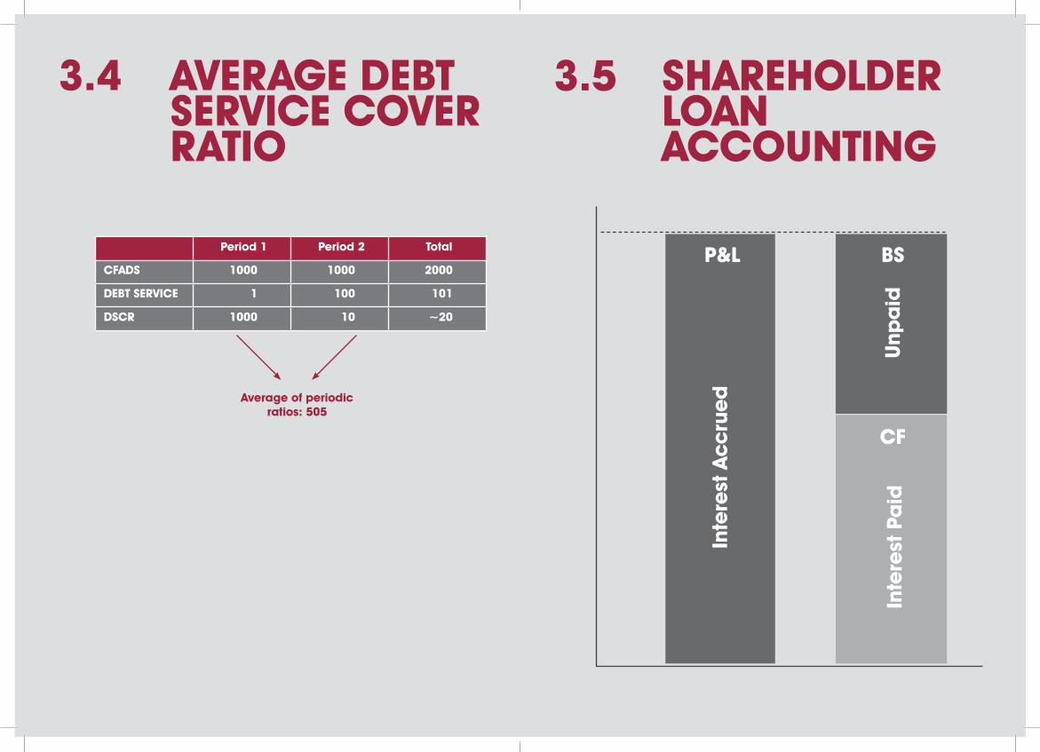
AVERAGE DEBTSERVICE COVERRATIO

3.4 SHAREHOLDERLOANACCOUNTING

3.5

Period 1 Period 2 Total

CFADS 1000 1000 2000

DEBT SERVICE 1 100 101

DSCR 1000 10 ~20

Average of periodic ratios: 505

P&L

Inte

rest

Ac

cru

ed

Inte

rest

Pa

idU

npa

id

BS

CF

30 31

DEBT SERVICECOVER RATIO

3.6 LLCR AS ‘TIMEVALUE’ DSCR

3.7

CFADS SUM(CFADS)* PV(CFADS)*

Cash Flow Available for Debt Service Average DSCR

Where PV(Debt Service) = Debt Balance

Hence LLCR=PV(CFADS) / Debt Balance

* Over debt term

Interest andPrincipal payments

Debt Service SUM(Debt Service) PV(Debt Service)

Measures flows, NOT balances.

SUM

LLCR

PV

32 33

NOTES: NOTES:

WWW.F1F9ACADEMY.COMWWW.F1F9ACADEMY.COM

34 35

NOTES: NOTES:


36 37

NOTES: NOTES:


38 39

NOTES: NOTES:



40

MODELLING NOTES

4NOTES:

WWW.F1F9ACADEMY.COM

42 43

Paste Quick Link & Row Anchor Alt , E , S , L ,

F2 , F4 , Enter

Copy Across Ctrl + C ,

Ctrl + Shift + Enter ,

Home , Shift + F9

Delete Sheet (Cannot Undo, make Alt, E, L

sure you are looking at a chart)

COMMON SEQUENCES

Beginning of row Home

Beginning of worksheet Ctrl + Home

Edge of data region Ctrl + <Arrow>

Last used cell in worksheet Ctrl + End

Vertically in worksheet PgUp / PgDn

Horizontally in worksheet Alt + PgUp / PgDn

Between worksheets Ctrl + PgUp / PgDn

Between workbooks / windows Ctrl + Tab

Between applications Alt + Tab

Jump to source of link Ctrl + [

Return from last jump F5 , Enter

Find / Replace Ctrl + F / Ctrl + H

Toggle help window Ctrl + F1

Close window / workbook Ctrl + W

Close application Alt + F4

NAVIGATIONQuick chart F11

Trace arrows Alt , T , U ...

Precedents T

Dependants D

Remove arrows A

Select row differences Select range -> Ctrl + \

Select column differences Select range -> Ctrl +

Shift + \

Display formulas in worksheet Ctrl + ¬

Paste name List F3, Alt + L

AUDITING & REVIEW

Copy & Paste (clears clipboard) Ctrl + C, Enter

Cut & Paste (clears clipboard) Ctrl + X, Enter

Paste special Alt , E , S ...

Formats T

Formulas F

Values V

All except borders X

Link L

Undo Ctrl + Z

Repeat Ctrl + Y or F4

Outline border on selection Ctrl + Shift + 7

Remove the borders Ctrl + Shift + -

EDITING: GENERAL

EXCEL 2003SHORTCUTS

4.1

44 45

Toggle edit and point mode F2

Toggle anchoring F4

Format cells dialog Ctrl + 1

Edit cell comment Shift + F2

SUM adjoining range Alt + =

EDITING: IN CELL

Select row Shift + SPACE

Select column Ctrl + SPACE

Insert new row Alt , I , R

Insert new column Alt , I , C

Insert copied selection Alt , I , E

Delete selection (row / column) Ctrl + -

EDITING: ROWS & COLUMNS

Worksheet Shift + F9

Workbook Ctrl + Alt + F9

Cell F2 , Enter

Individual formula element F2 , select element , F9

CALCULATIONS

4.1 EXCEL 2010SHORTCUTS

4.2

Beginning of row Home

Beginning of worksheet Ctrl + Home

Edge of data region Ctrl + <Arrow>

Last used cell in worksheet Ctrl + End

Vertically in worksheet PgUp / PgDn

Horizontally in worksheet Alt + PgUp / PgDn

Between worksheets Ctrl + PgUp / PgDn

Between workbooks / windows Ctrl + Tab

Between applications Alt + Tab

Jump to source of link Ctrl + [

Return from last jump F5 , Enter

Find / Replace Ctrl + F / Ctrl + H

Toggle ribbon visibility Ctrl + F1

Close window / workbook Ctrl + W

Close application Alt + F4

NAVIGATION

Paste Quick Link & Row Anchor Alt , H , V , N ,

F2 , F4 , Enter

Copy Across Ctrl + C ,

Ctrl + Shift + Enter ,

Home , Shift + F9

Delete Sheet (Cannot Undo, make Alt, E, L

sure you are looking at a chart)

COMMON SEQUENCES

46 47

Quick chart F11

Trace arrows Alt , M ...

Precedents P

Dependants D

Remove arrows A, A

Select row differences Select range -> Ctrl + \

Select column differences Select range -> Ctrl +

Shift + \

Display formulas in worksheet Ctrl + ¬

Paste name List F3, Alt + L

AUDITING & REVIEW4.2 Toggle edit and point mode F2

Toggle anchoring F4

Format cells dialog Ctrl + 1

Edit cell comment Shift + F2

SUM adjoining range Alt + =

EDITING: IN CELL

Select row Shift + SPACE

Select column Ctrl + SPACE

Insert new row Alt , H , I , R

Insert new column Alt , H , I , C

Insert copied selection Alt , H , I , E

Delete selection (row / column) Ctrl + -

EDITING: ROWS & COLUMNS

Worksheet Shift + F9

Workbook Ctrl + Alt + F9

Cell F2 , Enter

Individual formula element F2 , select element , F9

CALCULATIONS

Copy & Paste (clears clipboard) Ctrl + C, Enter

Cut & Paste (clears clipboard) Ctrl + X, Enter

Paste special Alt , H , V ...

Formats S , T

Formulas F

Values V

All except borders B

Link N

Undo Ctrl + Z

Repeat Ctrl + Y or F4

Outline border on selection Ctrl + Shift + 7

Remove the borders Ctrl + Shift + -

EDITING: GENERAL

48 49

EXCEL FORMATMACROS

4.3

Action Keyboard Shortcut Mnemonic Example

Normal Style Ctrl + Shift + , 000 separator (Comma) 10Factor Style Ctrl + Shift + . Decimal point key 10.0000

Increase 0s * Ctrl + . > for increase 10.0Decrease 0s * Ctrl + , < for decrease 10.00

Percent Style Ctrl + Shift + P P for Percent 10.00%

Toggle Date Style Ctrl + Shift + / / often used in dates 10 Jan 10

Update Format Styles Ctrl + Shift + L L used in styLes

NUMBER FORMATS

Action Keyboard Shortcut Mnemonic Example

Black Ctrl + Shift + B B for Black 10

Blue Ctrl + Shift + M M for iMport 10

Red Ctrl + Shift + X X for eXport 10

Border Ctrl + Shift + D D for unDerline 10

Square Brackets Ctrl + Shift + T T for Temporary [example]

COLOURS, BORDERS & TEXT

50 51

4.3Action Keyboard Shortcut Mnemonic Example

No shade Ctrl + Shift + C C for Clear 10

Red Ctrl + Shift + S S for Stop 10

Yellow Ctrl + Shift + Y Y for Yellow 10

Green Ctrl + Shift + G G for Green 10

Light Yellow Ctrl + Shift + I I for Inputs 10

Light Gray Ctrl + Shift + O O for cOunterflOws 10

Lime Ctrl + Shift + R R for Review 10

SHADING

Action Keyboard Shortcut Mnemonic

Jump to Precedent Ctrl + Shift + J J for Jump

Return from Jump Ctrl + Shift + K Next to J

NAVIGATION

NormalNumber: #,##0_);(#,##0);”- “;” “@Alignment: General, Top Aligned

CommaNumber: #,##0_);(#,##0);”- “;” “@Alignment: General, Top Aligned

FactorNumber: #,##0.0000_);(#,##0.0000);”- “;” “@Alignment: General, Top Aligned

STYLESPercentNumber: 0.00%_);-0.00%_);”- “;” “@Alignment: General, Top Aligned

Date ShortNumber: dd mmm yy_);;”- “;” “@Alignment: General, Top Aligned

Date LongNumber: dd mmm yyyy_);;”- “;” “@Alignment: General, Top Aligned

Note: Under “Style includes” untick all but “Number” and “Alignment” box when defining styles (to avoid changing anything but number and alignment format when applying styles.)

52 53

1. These macros have been:a) Designed to reside in a separate file, and not inside a spreadsheet itself (to avoid embedding non-essential macro's within a model)b) Saved in a "hidden" state (so that this file will not be in the way when you work). To unhide simply: Window, Unhide.To use these macros simply have this file open, albeit in a hidden state, when you are working in Excel.To have it open automatically when you start Excel just point your "Tools, Options, General (Tools, Options, Advanced, General for Excel 2007/2010),At start-up open all files" directory to it (making sure there are no unwanted files reside in the same directory).

2. To allow the above Number Formats and related Styles (see below) to work you first need to import the styles into your file.

You do this by:a) Unhiding this format macro file (Window, Unhide).b) From your spreadsheet import the style of this file, simply: Format, Styles, Merge, (Alt + H + J + M for Excel 2007/2010) selecting thename of this file OR simply press the shortcut key Ctrl + Shift + L.

3. Some keys require that a cell already has a valid numeric format. So if you get an error message then simply first ap-ply Comma style, then try again.

4. Finally please note that Excel's inbuilt "undo" memory is cleared each time you trigger a macro (not just these mac-ros, but any macro).

NOTES4.3 STANDARDPROCESSES

4.4

MODEL BUILD PROCESSES

‘COPYING ACROSS’ A FORMULA

1. Create the formula in column J. Then, in column J:

2. Control+C

3. Control+Shift+Right Arrow

4. Enter: to paste down the formula

5. Home

6. Shift+F9

4.4.1

4.4.1 ‘Copying across’ a formula4.4.2 Adding a row total4.4.3 Adding a Quick Chart4.4.4 Deleting a Quick Chart4.4.5 Creating a link4.4.6 Creating a link using ‘Paste Link’4.4.7 Navigating using links (Qwerty keyboards)4.4.8 Navigating using links (Non Qwerty keyboards)4.4.9 Copying and pasting an existing link4.4.10 Creating placeholders4.4.11 Marking an import (blue font)4.4.12 Marking an export (red font)

54 55

ADDING A ROW TOTAL1. Position your cursor in column H of the row of which

you want to show a total

2. Alt+=

3. Tap across and down until the cursor is positioned

in column J of that row

4. Shift+Ctrl+Right Arrow

5. Enter

ADDING A QUICK CHART1. Move the cursor to column J of the line you want

to chart

2. Shift+Control+Right arrow to select the range of

numbers to chart

3. F11. The chart is created in a new worksheet

DELETING A QUICK CHART

1. Control+S

2. In Excel 2007 and later: Alt,H,D,S

3. In Excel 2003: Alt,E,L

4. You will get a warning before you delete.

Make sure you are looking at the chart when

you delete the sheet

5. Enter

CREATING A LINK

1. Start from column E (i.e. place the cursor in

column E).

2. Type “=”into the column E cell

3. Using the Using the arrow keys, go to the row label

(in column E) of the calculation to which you want

to link

4. Tap F4 twice to row anchor the link

5. Copy across

(see ‘Copying across a formula’ p.41)

CREATING A LINK USING ‘PASTE LINK’

1. Start on the item to which you want to link

2. Ctrl+c on the label

3. Ctrl+Page Up/Page down to where you want to

place the link

4. Excel 2003: Alt, E, S, L, F2, F4, Enter

Excel 2007/10: Alt, H, V, N, F2, F4, Enter

NAVIGATING USING LINKS (QWERTY KEYBOARDS)

QWERTY keyboard

• Ctrl+[ takes you to the source of a link

• F5, Enter takes you back

4.4.2 4.4.5

4.4.6

4.4.7

4.4.3

4.4.4

56 57

NAVIGATING USING LINKS (NON QWERTY KEYBOARDS)

• Ctrl+Shift+J takes you to the source of a link

• Ctrl+Shift+K takes you back

COPYING AND PASTING AN EXISTING LINK

1. Shift+Spacebar to select the entire row of the link

you want to copy

2. Ctrl+C

3. move to where you want to put the new instance

of that link

4. Shift+Spacebar to select that row

5. Enter

CREATING PLACEHOLDERS

1. Ctrl+Spacebar to select the row

2. Ctrl+Shift+Y

3. Select the row label

4. Ctrls+Shift+T

5. Shift+F2 to insert a comment

6. Esc, Esc

4.4.8 4.4.11

4.4.124.4.9

4.4.10

MARKING AN IMPORT (BLUE FONT)

1. Ctrl+Spacebar selects the row

2. Ctrl+Shift+M

MARKING AN EXPORT (RED FONT)

1. Ctrl+Spacebar selects the row

2. Ctrl+Shift+X


58

TECHNICAL NOTES

5

60 61

5.1

5.1.1

THE MODELLINGOF INTEREST

INTRODUCTION

APPROXIMATION5.1.2

When a modelling period is longer than the underlying financial transaction period (i.e. the model’s time resolution is cruder than reality), financial calculations may suffer from either, or both of two modelling problems: approximation and/or circularity. By way of example, this discussion will be held purely with reference to interest expense during a debt draw period.

Specifically this note will:

1. Demonstrate that, when a modelling period is longer than the debt draw period, the most commonly used modelling approaches produce only an approximation of interest expense (Section 5.1.2).

2. Explain how modelling circularity arises in the context of forecasting interest expense and why circularity is a problem worth avoiding (Section 5.1.3).

3. Discuss non-circular modelling approximations of the circular ‘Average Balance’ approach (Section 5.1.4).

4. Present a non-circular Average Balance equivalent approach utilising a close-form mathematical solution (Section 5.1.5).

Let us assume we have an annual, calendar year model (i.e. each spreadsheet column represents one calendar year). So, for modelling purposes we are limiting ourselves to working with only one debt draw, one debt balance, one interest rate and one interest expense per year. As far as assigning a specific date against this single calendar year modelling period, we opt for the end of the period (commonly known as the ‘end-of-period’ convention), namely 31 December. Finally, let us assume that in reality the transaction we are modelling has semi-annual debt draws (i.e. twice during any given modelling period).

A representative period, the year 2002, is diagrammed below, with a balance at the end of the previous modelling period (31 Dec 2001) of £10 million, a draw mid-way through 2002 (30 June 2002) of £5.0 million and a further £5.0 million draw at the end of the current modelling period (31 Dec 2002). Assuming an interest rate of 10% p.a. (on a 6 month interest payment period basis, so 5% for each semi-annual period), the accurate forecast of interest expense for 2002 is £1.25 million.

Leaving interest compounding issues aside for simplicity,1 how does this accurate interest expense forecast compare with two of the simplest and most commonly used modelling approaches?

Before answering this question, let us remind ourselves that we only have one draw and one point in time (to measure a balance) available to us per modelling period. In the above annual model example, we therefore only have available a draw amount for the full year 2002, a balance as of 31 Dec 2001 (which on our end-of-period convention, we can refer to as the ‘ending balance of the previous period’) and the balance and draw as of 31 Dec 2002 (which we will refer to as the ‘ending balance of the current period’). The 30 Jun 2002 draw of £5.0 million and balance of £15.0 million do not exist in our modelling example. To add to the confusion, the ending balance of the previous period is (always) equivalent to the ‘beginning balance of the current period’.2

62 63

Annual Model, Semi-Annual Reality

The example outlined in Figure 1 combined with the above nomenclature leads to the somewhat common spreadsheet representation provided in Figure 2 below. Though ‘calculations’ are shown for three periods/columns (E through G), Column F, representing the year ending 31 Dec 2002, is really the only period for which information is available. (Columns E and G, which note ending and beginning balances respectively, are presented solely to demonstrate the equivalency between the beginning balance and the previous period’s ending balance. This relationship explains why this calculation structure is sometimes referred to as a debt balance ‘corkscrew.’)

One somewhat intuitive modelling approach to this problem of ‘missing information’ (i.e. the intermediate balance on 30 Jun 2002) is to assume that the full amount of draws for the relevant period are made at a single point in time sometime during the relevant period. The most obvious and common assumption is that these draws are made mid-period (the so-called ‘Mid-Period Draw’ Approximation). Interest is accrued on the drawn amount for half the period (and of course on the beginning balance for the entire period)

It works out algebraically that this Mid-Period Draw Approximation is functionally equivalent to assuming that equal draws are made continuously throughout the period, such that balance profile follows a straight line (not stepped) between beginning and ending Balance. The effective interest accrued under these circumstances would be calculated on the average of the beginning and ending Balances (and is therefore sometimes referred to as the ‘Average Balance’ approximation).3 Noting that the beginning balance is £10.0 million (31 Dec 2001) and the ending balance is £20.0 million (31 Dec 2002), this approach yields £1.50 million (i.e. £10.0 + £20.0 million divided by 2 at 10%) in interest.

For those situations where the Average Balance approach causes a modelling circularity (the topic of Section 3.0 below), the simplest non-circular alternative to the Average Balance approach is what is known as the ‘Beginning Balance’ approach, namely calculating interest using the ending balance of the previous period. Or put another way, assuming that the entire draw occurs at the end of the period. This approach yields £1.00 million (i.e. £10.0 million at 10%). (A further elaboration on the typical logic diagram for this simplified ‘Beginning Balance’ approach is detailed in Annex A.)

Whereas the calculation using the Beginning Balance approach predictably (in our example) underestimates interest (by £250,000), we somewhat surprisingly see that the Average Balance approach overestimates it by an identical amount (i.e. £250,000). While this symmetry around the correct answer is somewhat coincidental, we nevertheless see that the commonly considered ‘correct’ Average Balance approach is materially inaccurate.

£ millions

31 Dec 2001 30 Jun 2002 31 Dec 2002

£5 million draw

£5 million draw

20

15

5

10

(Fig.2)

(Fig.1)

5.1.2 5.1.2

64 65

In short, in situations where the modelling period is longer than the debt draw period, the most commonly used modelling approaches only provide an approximation of interest expense. (Annex E provides a more detailed analysis of the levels of inaccuracy in the two approaches for various combinations of modelling periods to actual draw periods.)

5.1.3 CIRCULARITYOne common financial forecasting challenge is minimising, and ideally eliminating, modelling circularity, meaning that circularities rarely (if indeed ever) exist in reality. It is only through the exercise of ‘modelling future financial reality’ (a.k.a. financial modelling) that analytical circularity arises.

Modelling circularity is worth avoiding for the following reasons:

1. The circularity ‘prompt’ is one of the few (and arguably most valuable) in-built quality control features available within spreadsheet software. However, once one circularity is accepted (through working in iterative calculation mode), this quality control feature is lost as subsequent unintended circularities will not be reported.

2. While there are ‘manual fixes’ to working with circularity that may retain this ‘prompting’ capability, these techniques involve either i) creating a macro or ii) regularly removing the known circularity (in order to check for new, unintended circularities). As such, these techniques are complex, non-transparent, and/or laborious.

3. Spreadsheets are notoriously bad at finding the origin of a circularity. Therefore unless the circularity is dealt with as soon as it presents itself, the effort involved in finding it later is considerable (see the ‘Flushing out Circularity’ slides as part of the Modelling 101 course). Finding multiple, unintentional circularities is almost impossible (particularly when the modeler has only recently ‘picked up’ the model in question).

This ‘multiple circularity’ risk may also apply to the technique of manual, periodic removal described in the preceding paragraph, since the modeler will be ‘stuck’ if he/she has unintentionally introduced more than one new circularity since the model was last so checked.

4. By working in iterative calculation mode, model calculation time is increased by a factor equal to the number of iterations necessary to reach an equilibrium (usually 5 to 6). In large models, this could mean increasing calculation time from, say, 20 seconds to 2 minutes. This calculation speed problem applies to both the ‘manual fixes’ options described in No. 2 above.

5. In models of the size and complexity used commonly in the finance industry, current versions of Excel are erratic at notifying the user of circularity. For this reason alone, working with circularity should be avoided if at all possible.

6. Finally, modelling circularity is occasionally purely a product of sloppy thinking and can often be eliminated simply through better (not larger, nor more complex) modelling of a particular element.

One common instance of modelling circularity involves trying to model a financing cost that in reality relates to draws within a modelling period (mid-way through the modelling period in our example above), and where the financing costs in turn relate to these intra-period draws.

A typical example is the Average Balance approach to the modelling of interest expense during a debt draw period (as shown in the diagram in Section 2.0 above), provided we add the assumption that (amongst other costs) debt draws are made in order to fund interest expense itself (or a proportion of it). Thus whereas the use of the Average Balance approach is driven by a mismatch between the modelling period and reality, the circularity arises only through a combination of i) adopting the Average Balance approach and ii) the use of debt draws to fund interest expense. (Please refer to Appendix A for the algebraic demonstration of circularity in this instance.)

66 67

While on the above assumption, the Average Balance approach creates a modelling circularity (because the ending balance of the current modelling period includes a draw to fund interest itself), the ‘accuracy’ benefit of this approach is commonly judged to outweigh the cost of living with a circular model. Yet as we saw in the worked example in Section 2.0 above, the circular Average Balance approach can be just as inaccurate as the non-circular Beginning Balance approach. However, since prudent modelling forecasts (i.e. overestimates) are generally preferred (from both a debt and equity perspective), the Average Balance approach normally ‘wins out’.

With the balance applicable to the calculation of commitment fees being a function of the balance used for the calculation of interest (i.e. debt commitment amount minus debt drawn equals the committed, but un-drawn, balance used in calculating commitment fees), the above (and subsequent) arguments apply equally to the calculation of commitment fees. For simplicity, however, commitment fees will be ignored in the remainder of this discussion.

5.1.3 5.1.4 NON-CIRCULARAPPROXIMATIONS OF AVERAGE BALANCEOn the basis that circularity should be avoided if at all possible, let us explore two reasonably intuitive non-circular alternatives to the circular Average Balance approach. These both produce a more prudent (but still inaccurate) forecast compared to the non-circular Beginning Balance approach. Both approaches below are essentially variations on the Average Balance approach, but each relies on creating a ‘synthetic’, non-circular ending balance in replacement of the actual modelling period ending balance (the latter causing the circularity in the Average Balance approach).

1. Capital Cost Only. Make the synthetic ending balance a ‘capital cost only’ balance by calculating draws for the period as i) the capital costs for the period, multiplied by ii) the debt ratio. This excludes from the ending balance all financing costs related to intra-period draws from the current period, the most significant of which being interest expense, and hence the ending balance calculated from these elements will not cause a circularity. This is a reasonably solid approach, but obviously suffers from ignoring all financing costs in the approximation.

2. Non-Circular Uses of Funds.4 The Capital Cost Only approach can be enhanced by incorporating two modifications:

a. adding other (non-circular) financing costs such as up-front fees and agent bank fees to the synthetic ending balance; and

b. adding interest expense based on the Beginning Balance approach (i.e. a non-circular interest expense approximation) to the synthetic ending balance.

68 69

Having made the above modifications, the only difference left (in terms of result) between the Non-Circular Uses of Funds approach above and the circular Average Balance approach is the effect of interest compounding within the modelling period.5 (‘Interest on interest’ is ‘solved’ by working in iterative calculation mode with a circularity.)

5.1.4

5.1.5 NON-CIRCULAR AVERAGEBALANCE MATHSThe Average Balance circularity can be solved algebraically and applied to a financial model with what, in mathematics, is generally referred to as a closed-form solution. Specifically, we can calculate a factor to apply to the non-circular Uses of Funds (UNC), the so-called “p” factor derived in Annex C, as follows:6

p = 2k / (2 – ki)

where:

k = debt factor (percentage of debt to total sources of funds);7 and

i = interest rate

Working from the example from Figure 1, we can see how this factor would be applied in a financial model. The Non-Circular Uses of Funds approach summarised in Section 4 relies on two components: i) interest calculated on the beginning balance (only), or £1.0 million in this example; and a Non-Circular Uses of Funds (i.e. Uses of Funds excluding interest), or UNC.

If we assume that the percentage of uses funded by debt (the leverage, “k”) is equal to 75%, then the total Uses of Funds for the year in question would equal the £10.0 million total draw over the year divided by 75% or £13.33 million. Assume for a minute we did know that the interest we were trying to calculate (albeit incorrectly) was based on

the Average Balance approach, and hence £1.5 million. This would imply that the remaining non-interest elements of the Uses of Funds in this example were £11.83 million (i.e. UNC = £11.83 million).

With a 10% interest rate and 75% leverage (“k”), the “p” factor equals 0.7792. Applying this factor to the sum of the two components (£1.0 million + £11.83 million), neither element including interest on amounts drawn during the period), yields a total draw of £10.0 million. Using this as the ‘non-circular’ draw will yield the Average Balance interest expense approximation of £1.5 million.

Thus if one is willing to adopt the above amount of mathematical sophistication, there is no need to explore circular Average Balance alternatives. Working from the basic framework introduced in Annex A, Annex D overviews the logic sequence needed to adopt this ‘non-circular’ Average Balance approach.

Just remember: the answer is still wrong.

70 71

5.1.6 TAKING THE ‘P’ FACTOR ASTEP FURTHER

The preceding use of the “p” factor to calculate a non-circular method for the Average Balance Approach seems like an awful lot of maths and effort for an answer which, in the end, is often a poor approximation. Can we use the “p” factor approach to yield a better approximation? We noted earlier that the Average Balance was functionally equivalent to assuming that total drawn amount occurs mid-period. However, in the case of annual modelling of a semi-annual debt draws, a far better approximation would be to assume that half the draws accrue interest for half the period, and the other half accrue no interest at all (since they occur at the end of the period). The equivalent to saying that half the draws accrue interest for half the period is to say that the total draws essentially accrue interest for one quarter of the period, or that the total draw occurs three quarters the way through the period. If we could calculate the drawn amount (without a circularity), then use this approach, we might be very close to the semi-annual reality. To see how this might work is best illustrated by developing the example in Figure 1 a bit further. First off, the reality of modelling is that debt draws will most likely be calculated by the financial model, not simply given as they have been in Figure 1. What will typically be given (as inputs or otherwise calculated elsewhere in the model independently ) are those uses of funds not related to interest. For this example, let’s assume these are restricted to “Capital Costs” only.8 Let’s assume for the two six-month periods used in Figure 1 that we have been given Capital Costs of £6.167 million and £5.916 million respectively. Furthermore, let’s assume that debt funds 75% of these costs, as well as 75% of any accrued interest. All other assumptions are as per Figure 1. This example would yield a ‘tabular’ version of this reality consistent with (which as it happens is consistent with the information ‘calculated’ in Figure 1).

6-month Period Ending

30 Jun 2002 31 Dec 2002 Total

(A) Beginning Balance previous (F) 10,000 15,000

(B) Capital Costs Input 6,167 5,916 12,083

(C) Interest (A) * 10% / 2 500 750 1,250

(D) Uses of Funds (B) + (C) 6,667 6,666 13,333

(E) Debt Draws (D) * 75% 5,000 5,000 10,000

(F) Ending Balance (A) + (E) 15,000 20,000

If our model was set-up with semi-annual precision, it would be a simple matter to model the logic outlined in Table 1 directly (and in fact this is often the recommended approach). However in an annual model, we are faced with calculating this total interest (£1.25 million) in one column (not two). Of course there are a number of approaches described above, including the Average Balance (or Mid-Period Draw) Approximation. However, is it possible to calculate a better estimate of this interest than what this would yield (i.e. £1.5 million or 20% higher than the actual amount). Annex F derives an ‘enhanced’ “p” factor (“p(r)”) that relates to the ‘effective’ proportion of the period over which interest on the (total) draws for the period actually accrues (“r”), which is:

p(r) = k / (1 – kir) 9

where “i” is the effective modelling period interest rate and “k” is the proportion of uses funded by debt (commonly referred to as ‘leverage’). Hence for our example, where we assumed r = 0.25, the enhanced “p” factor is 0.764310 Revisiting Table 1, but this time restricting ourselves to our hypothetical annual model yields the approach for calculating interest outlined in Table 2.

Table 1/ Note: All figures in GBP 000s

72 73

Year Ending 31 Dec 2002

(A) Beginning Balance previous (F) 10,000

(B) Capital Costs Input 12,083

(C) Interest (on beginning balance only) 10% * (A) 1,000

(D) Non-Circular Uses of Funds (UNC) (B) + (C) 13,083

(E) Non-Circular Debt Draws p(r) * (D) 10,000

(F) Interest (on intermediate draws)(E) * 10% * 0.25, i.e. effective time over which draws accrue interest

250

(G) Interest (total) (C) + (F) 1,250

(H) Uses of Funds (B) + (G) 13,333

(I) Debt Draws (E), or alternately k * (H) 10,000

(J) Ending Balance (A) + (I) 20,000

In this particular case, the reader will note the ‘approximation’ is in fact identical to the actual target figure reported in Figure 1 (and as calculated semi-annually in Table 1). Unfortunately, in most cases, this will not be the case, since this equivalency ties to the unusual circumstance that both draws during the period were equal, and hence the estimate of r = 0.25 was precisely correct. Nevertheless, in most cases, application of the enhanced “p” factor will yield an answer closer to reality, particularly where the draws over the period are reasonably even.

5.1.6

Table 2/ Note: All figures in GBP 000s

5.1.7 CONCLUSIONS

The foregoing leads to the following conclusions:

1. When a modelling period is longer than the underlying financial transaction period, commonly used modelling approaches will generally only produce an approximation of the variable being calculated. One such example is interest expense related to debt draws, where the Beginning Balance approach underestimates interest expense and Average Balance approach overestimates interest expense. (Note: the reverse applies to debt repayment periods.)

2. The only way to ensure modelling an accurate amount of interest expense is to make the modelling period equal to (or shorter than) the interest payment period.11 While this modelling approach is of course legitimate, it generally requires i) sophisticated logic to handle worksheets with different time periods (e.g. monthly sheets and semi-annual sheets), and/or ii) a significantly larger model.

3. Circularity should, and can often, be avoided. In the case of the Average Balance approach to interest expense calculation, avoiding circularity entails using the close-form mathematical set out in Section 5.0 above (or it’s enhanced version outlined in Section 6.0). The primary (and serious) drawback of this approach is that the equation looks ‘strange’ and the derivation/explanation is mathematically complex. This will likely lead to a lack of modelling ‘transparency’ that must somehow be addressed (e.g. via some lengthy explanatory comment that should be included in the model concerning the calculation).

4. Choosing which approximation approach to use may depend on the circumstances of actual and modelling draw periods. As detailed in the tables of Annex E, the inaccuracy of the Average Balance approach (a.k.a. Mid-Period Draw Approximation) decreases with relatively more frequent actual draw periods, and it is further somewhat resistant to the chosen modelling period (immune if the draws are equal). With appropriate

74 75

programming logic, the Beginning Balance approach should always be used whenever the modelling period is equal to or shorter than the actual draw period. Otherwise, the magnitude of the error with the Average Balance approach is often smaller.

Given the above, F1F9 Academy recommends either i) building a model with a period equal to or shorter than the required compounding period (and of course using a Beginning Balance approach), or ii) using an Average Balance approach, ideally as enhanced pursuant to the description in Section 6.0. Even with a relatively high resolution quarterly model, calculating interest expense on a Beginning Balance basis (when the underlying debt draw period is monthly) is: i) less accurate than the Average Balance approach and ii) an underestimate of the accurate figure (see Annex E for the specific figures in the example outlined).

5.1.7 ANNEX A5.1.8

One of the more difficult areas of financial modelling involves calculating cash flows during a draw-down period, most often during a construction period for the project/company in question. This complexity arises when financing charges are funded from further draws of debt funding (there being yet no revenues from commercial operations), and this structure leads to a certain ‘circularity’ in the logic.

Whether this conceptual circularity manifests itself into a technical Excel logic circularity depends on whether cash flows in a particular period in turn rely on values that involve amounts calculated in that period (rather than on values from the previous period or independent inputs).

‘BEGINNING BALANCE’ INTEREST CALCULATION

76 77

The preceding schematic helps to demonstrate the logic flow for a typical, non-circular funding structure in which debt and equity are funded as a constant, pro rata percentage of Uses of Funds.

At first glance the logic may appear ‘circular’ because the logic arrows form a closed-circuit. However, the following walk-through demonstrates why this logic will not cause an actual circularity (a.k.a. CIRC) in the spreadsheet logic. (The numbered balloons conform to the following logic steps.)

1. Upfront Fees, Agent Bank Fees, and Debt Service Reserve Fund Deposits are calculated (each of which in this set-up depends on independent inputs). For the time being, Interest during Construction (IDC) and Commitment Fees are ignored.

2. The preceding ‘non-balance related’ financing costs are combined with Capital Costs to derive a provisional Uses of Funds.

3. By definition, Uses of Funds equal Sources of Funds.

4. A percentage (based on a Leverage Percentage Input) of this preceding provisional Sources of Funds is funded from Debt Draws, with the remainder coming from Equity Investment.

5. These (still provisional) Debt Draws allow an initial debt balance ‘corkscrew’ to be set up, in which the Beginning Debt Balance relates only to the Ending Debt Balance of the previous period.

6. This Beginning Balance in turn can be used to calculate beginning-balance related IDC and Commitment Fees, which in turn are “hooked into” the Financing Costs sub-total and the logic is complete.

The arrow from No. 5 to No. 6 seems to (and does in a way) ‘complete a circle’. However, the Beginning Balance

relates only to the previous period amounts, and therefore no circularity is created. The logic diagrammed is more of a spiral than a circle (in effect a large ‘corkscrew’).

Also from the preceding analysis it can be seen that if the ‘Average Balance’ (i.e. average of Beginning and Ending Balances) was used as the basis of the IDC and Commitment Fee calculations, that the logic so constructed would generate a circularity. This is because the Ending Balance relates to debt draws of the current period, which in turn are a percentage of Sources (and Uses of Funds). Uses of Funds in turn relate to Financing Costs, which include IDC and Commitment Fees, which relate to the Ending Balance (by way of the Average Balance calculation). Therefore, the Average Balance approach simply applied via this method completes a circular loop within the current period (i.e. a loop within the same Excel column).

5.1.8 5.1.8

78 79

ANNEX B ANNEX C5.1.9 5.1.10THE ALGEBRA OF CIRCULARITY

THE ALGEBRA OF NON-CIRCULAR AVERAGE BALANCE

5.1.10.1

The circularity of using the “average balance” to calculate interest can be shown algebraically in the following equations, where:12

B = Beginning debt balance E = Ending debt balance I = Interest expense i = interest rate U = Uses of funds

UNI = ‘No-interest’ uses of funds * *Capital costs and non-interest expense financing costs (i.e. Uses of Funds excluding interest and commitment fees, the latter being ignored in this derivation).

k = debt factor (percentage of debt to total sources of funds)

D = Draws for the period

In this case: I = i * average balance

= i(B + E) / 2

where: E = B + D = B + kU

= B + k(UNI + I)

Therefore, unless some further work is done, this creates a circularity, as

I = f(E) and

E = f(I) so

I = f(I)

where f() simply represents“function of” the relevant variable (among others).

To get behind the algebra in Section 5.0 requires working through some off-line algebra. Picking up with the designations and relationships identified in Annex B yields:

E = B + k(UNI + I)

= B + k * {UNI + i(B + E) / 2}

= B + kUNI + kiB / 2 + kiE / 2

or, grouping the “E” terms to the left side:

E - kiE / 2 = B + kUNI + kiB / 2

E(1 - ki/2) = B(1 + ki / 2) + kUNI

multiplying both sides through by 2:

E(2 - ki) = B(2 + ki) + 2kUNI

or

(A)E = (2 + ki)B + 2kUNI

(2 - ki)

Therefore, rewriting the traditional (and direct) formula for ending balance equalling beginning balance plus draws to this equations removes the circularity. Ending balance (“E”) need not be a function of interest, and once calculated, interest (and other terms) can be calculated without producing a circularity.

80 81

DERIVATION OF THE ‘P’ FACTOR5.1.10.2 5.1.10.2

The preceding approach has a fundamental weakness, which is the formula for the ending debt balance during the construction phase certainly does not leap out as being obvious, and hence a financial model adopting this approach will lack transparency. In short, anyone reviewing this logic will wonder what is going on and/or have to walk through some considerable comments and explanations. What if the Non-Circular Uses of Funds approach in Section 4.0 above could be combined with the solution above?

The Non-Circular Uses of Funds approach relies on calculating an estimate of Uses of Funds, excluding those terms that would create a circular reference, and calculating interest on the beginning balance only. We will call this the ‘No-Circ’ Uses of Funds or UNC.

13

UNC = UNI + iB

where, as noted in Annex B, UNI are those uses of funds not relying on debt balances (e.g. capital costs, agent bank fees, up-front fees, etc.) and excluding interest.

A proportion of UNC is then taken as the estimated debt draws. This proportion (“p”) is clearly approximated by the percentage of debt, but because of intra-period compounding, this is not exactly right. So what is the “right” factor?

Taking the solution for ending balance (“E”) in the preceding section (Equation “A”) as a starting point:

E = (2 + ki)B + 2kUNI

(2 - ki)

actual draws (“D”) can be calculated as

D = E - B

= (2 + ki)B + 2kUNI

(2 - ki)

which can be simplified to:

D = 2B + kiB + 2kUNI - (2 - ki)B

(2 - ki)

= 2B - 2B + kiB + kiB + 2kUNI

(2 - ki)

= 2kiB + 2kUNI

(2 - ki)

= 2k(UNI + iB)

(2 - ki)

and therefore from inspection, the proportion of UNC (i.e. UNI + iB) to take as the debt draws is the “p” factor:

p = 2k / (2 – ki)

- B

82 83

ANNEX D5.1.11NON-CIRCULAR AVERAGE BALANCE LOGICAnnex A demonstrated that directly calculating an Average Balance and applying this to IDC and Commitment Fees leads to a logic circularity (which should be avoided at all costs). However, being more careful with the logic construction and applying the p-factor derived in Annex C can lead to a ‘non-circular’ Average Balance alternative.

The logic diagram (next page) shows how this can be accomplished in the following (labelled) steps:

1. As with Annex A, begin with those financing costs that rely only on independent inputs (i.e. do not relate to calculated balances). In the Modelling 101 Training Model upon which this logic is based, these ‘non-balance’ costs include Upfront Fees, Agent Bank Fees, and (Initial) Debt Service Reserve Fund Deposits.

2. Calculate the ‘No-Circ’ Uses of Funds line item (UNC referenced in Annexes B and C) from the preceding ‘non-interest’ financing costs, Capital Costs, and a ‘No-Circ’ IDC (i.e. interest calculated based on the beginning balance only). (Note, as is the case throughout this note, Commitment Fees are not included in the algebra or this flow diagram in this sense.)

3. Apply the p-factor to these ‘No-Circ’ Uses of Funds to derive a so-called ‘no-circ’ Debt Draws from which one can calculate a non-circular based debt balance corkscrew.

4. Then calculate the No-Circ Average Balance from the preceding corkscrew, and use it as the basis for IDC and Commitment Fees.

84 85

5. From here, calculate the Financing Cost sub-total from its (five) constituent parts.

6. Calculate Uses of Funds as the sum of Capital Costs and Financing Costs

7. Sources of Funds equals Uses of Funds

8. Calculate Debt Draws as the leverage percentage (an input) of Sources of Funds and construct the debt balance corkscrew. Note that it is the Beginning Balance from this corkscrew that forms the basis for the ‘No-Circ’ IDC used in the No-Circ Uses of Funds referenced in Step No. 2.

5.1.11 ANNEX E5.1.12BEGINNING AND AVERAGE BALANCE APPROXIMATIONS

Tables E-1 and E-2 below present the amount of error introduced in the Beginning and Average Balance Approximations (respectively) for combinations of modelling period resolution to actual draw periods. The figures are calculated as the difference in interest between the actual amount and each of these approximations using the parameters of the example of Figure 1.14 In looking at a simple 12-month span of time (as was done in the example in the main text), periods of 1, 2, 3, 4, 6, and 12 months are ‘valid’, meaning they divide evenly into the 12-month period over which interest is calculation. In each case, the combination of a 6-month Actual period with a 12-month Modelling period outlined in the main text is highlighted.

Beginning Balance less Actual Interest Differences (GBP 000s)*

Modelling Period

Actual Period 1 month 2 months 3 months 4 months 6 months 12 months

1 month - (42) (83) (125) (208) (458)

2 months - - (42) (83) (167) (417)

3 months - - - (42) (125) (375)

4 months - - - - (83) (333)

6 months - - - - - (250)

12 months - - - - - -

Table E-1 /

*Negative figures (in parentheses) mean that approximation under-estimates correct answer

86 87

Average Balance less Actual Interest Differences (GBP 000s)

Modelling Period

Actual Period 1 month 2 months 3 months 4 months 6 months 12 months

1 month 42 42 42 42 42 42

2 months 83 83 83 83 83 83

3 months 125 125 125 125 125 125

4 months 167 167 167 167 167 167

6 months 250 250 250 250 250 250

12 months 500 500 500 500 500 500

5.12 5.12

Table E-2 /

From Tables E-1 & E-2, the following conclusions can be drawn:

1. For a given actual period being modelled, the degree of inaccuracy in the Average Balance approximation is immune to the modelling period. This may be somewhat intuitive, as in effect the average balance takes a ‘straight line’ approximation in estimating the appropriate balance for applying interest.15

2. The straight-line, or continuous draw, approximation underlying the Average Balance approximation suggests that the error should approach zero as the actual draw period becomes shorter and shorter. This is supported by the figures in Table E-2.

3. In all cases where the modelling period is at an equal or higher resolution than the actual draw frequency, the Beginning Balance can be modelled accurately. (In those cases where the modelling frequency is higher, certain columns will need to be ‘skipped’, best done by multiplying by a ‘draw flag’ of some sort.)

4. The cases in which the Beginning Balance approach under-estimates the actual amount by the same magnitude as the Average Balance over-estimates (which includes the example combination) are those cases in which the modell:actual periods are in a ratio of 2:1 (e.g. a 6-month modelling period estimating a 3-month actual draw period).

5, As the ‘reality’ to ‘modelling’ period ratio increases (i.e. the simpler/cruder the model gets) the relatively less inaccurate the Average Balance approach becomes (perhaps the case with the Modelling 101 Training Model). For instance in the example used, an annual (12-monthly) model approximating a monthly (equal) draw frequency, the Average Balance over-estimates the ‘true’ answer by £42,000, whereas the Beginning Balance approach under-estimates by £458,000.

While there are few absolute conclusions from the preceding analysis, it provides some picture of the behaviour of the two approximations and may provide some guidance as to which is least worst under various circumstances.

88 89

1 When working from a semi-annual interest input in an annual model (which is typically reported on a simple per annum, not compounded, basis), one should typically annualise the interest rate (e.g. 5% paid semi- annually is equivalent to 10.25% paid annually).

2 Put another way, the balance on the last second of 31 December 2001 (ending balance of previous period) is identical to the opening/beginning balance as at the first second of 1 January 2002 (beginning balance of the current period).

3 The term ‘Average Balance’ is arguably a misnomer, since it suggests an amount which is representative of the amount outstanding over a period (and therefore the correct ‘volume’ on which to apply the rate of interest). This is only true in the fictional assumption of infinitesimally small draws made on an infinitely frequent basis. In our actual example, £10.0 million is outstanding for the first half of the year and £15.0 million for the second (only increasing to £20.0 million in the ‘last second’), and hence the actual (time-weighted) average balance is more properly £12.5 million. The ‘Average Balance’ as we use it in this note ought to be known as the ‘the average of the ending balance and the beginning balance of the period’, but we have mercifully shortened this.

In fact applying the interest rate to this proper time-weighted average balance would in fact yield an accurate interest calculation. The reader may query whether this average can/could in fact be calculated. In this simple example of two equal £5.0 million draws (and with no interest compounding issues), perhaps (as we shall see in Section 6.0), but in more typical ‘real life’ examples this becomes impractical without increasing the resolution of the modelling period.

4 Uses of Funds is defined as Capital Cost plus Financing Costs.

5 This statement is true only if it is assumed that interest expense is the only “draw-related” financing cost (i.e. other such charges, such as commitment fees, are ignored for purposes of this discussion).

6 Annex C picks up on the designations and relationships identified in Annex B. Therefore it is advisable to look at Annex B before reviewing Annex C.

7 Note for this particular construction to be valid, the algebra relies on the assumption that debt is drawn as a constant (i.e. pro rata) percentage of Uses of Funds (i.e. leverage percentage “k”). Other financial structures are likely (at best) to require substantially less ‘clean looking’ solutions.

8 For purposes of this example, this is a simplified label. This amount could also contain other, often financing, costs unrelated to interest (say bank up-front fees). Hence the Annexes typically use the Capital Costs together with these other costs in calculating so-called non-circular uses of funds (“UNC”). The modelling approach to include simply requires these additional uses of funds be added to Capital Costs.

9 One may note that the ‘r’ factor for the assumption that all draws occur at the end of a period (hence a beginning balance approximation being ‘correct’), is r = 0, and hence the ‘p factor’ is simply equal to the leverage ‘k’. As one would hope/expect, this will in fact yield Non-Circular Debt Draws equal to actual draws (as/if actual draws include only interest based on the beginning balance).

10 The ‘r factor’ is easier to describe by way of example (as we have done in the text), than with a label, at least a short one. The best ‘sense’ for the ‘r’ factor’s definition is, “The best estimate of the time-weighted ‘presence’ of total draws during period, as this relates to the impact on interest accrued on these draws during the period (i.e. excluding interest accrued on the beginning balance for the period).”

11 Saying that anything in a model is “accurate” is always dangerous. In part this due to the reality of forecasting error, but also relates to issues of modelling expediency/precision. For instance, it is rarely justified to include rounding logic to reflect loan agreement stipulations that draws must be made to the nearest £1 million.

12 For simplicity, commitment fees, which also relate to debt balances during the period, are ignored. However, the principles discussed herein can be expanded to include these charges in the approach.

13 Note again that commitment fees are ignored from this calculation.

14 The particular assumptions are a £10.0 million opening balance, £10.0 million in additional debt draws over the 12-month period, divided equally into howsoever many periods, and a 10.0% p.a. interest rate, as with the example in the text, divided simply.

15 Rather than the true time-weighted average balance described in the footnotes of the main text, the Average Balance assumes a continuously smooth, not ‘stepped’ draw profile, such that the average balance is equal to average of the two sides (similar to calculating the area of a trapezoid).

ANNEX F END NOTES5.1.13 5.1.14DERIVATION OF THE ENHANCED ‘P’ FACTOR

As has been reviewed elsewhere in this note, total draws can be rather simply thought of as the debt proportion (“k”) of total uses of funds, where in turn uses of funds can be split between i) those uses of funds not related to interest (“UNC”) plus ii) total interest (“I”).

What if we re-visit Annex C, but this time assume that interest (“I”) can be better approximated by the expression:

I = i(B + rD)

where r is the ‘effective’ fraction of the period for which the modeler believes interest accrues on the total drawn amount (“D”). As noted in the text, for annual modelling of a semi-annual debt structure, r would be one quarter or 0.25.

Putting these thoughts together yields the expression:

D = k(UNC + I)

= kUNC + ki(B + rD)

= kUNC + kiB + kirD

Bringing the last “D” term over to the right side of the equation yields:

D - kirD = kUNC + kiB

D(1 - kir) = k(iB + UNC)

or

D = k(iB + UNC) / (1 - kir)

Hence, by inspection, the ‘enhanced’ p-factor (i.e the coefficient of iB + UNC), which vary depending on the modeler’s judgement of “r” is is equal to:

p(r) = k / (1 - kir)

Since the values of k, i, B, UNC and r are all known at the start of the current modelling period, calculating draws on this basis will not create an Excel circularity.Note: replacing r with ½ (which is the assumption in the Mid-Period, or alternately the Average Balance Approximation) and multiplying the top and bottom of the expression through by 2 yields the expression for the “p” factor provided in Annex C.

FAST PROJECT FINANCE MODELLING

Documents

Transcript of FAST PROJECT FINANCE MODELLING