Introduction to Fast Fourier Transform inFinance

Ale� µCerný

Tanaka Business School, Imperial College London, South Kensington Campus,SW7 2AZ, London, UK. Phone ++44 20 7594 9185. Fax ++44 20 7823 7685.

a.cerny@imperial.ac.uk

First draft: July 2003Revised: 18th June 2004

Typos in eqs. (38-40) corrected 20th February 2006

Abstract

The Fourier transform is an important tool in Financial Economics. It delivers realtime pricing while allowing for a realistic structure of asset returns, taking intoaccount excess kurtosis and stochastic volatility. Fourier transform is also ratherabstract and therefore o¤-putting to many practitioners. The purpose of this paperis to explain the working of the fast Fourier transform in the familiar binomial optionpricing model. We argue that a good understanding of FFT requires no more thansome high school mathematics and familiarity with roulette, bicycle wheel, or asimilar circular object divided into equally sized segments. The returns to such asmall intellectual investment are overwhelming.

Key words: fast Fourier transform, option pricing, binomial lattice, chirp-ztransform, GAUSS, MATLAB

JEL classi�cation code: C63, G12

Mathematics subject classi�cation: 65T50, 91B70, 91B24

The Fourier transform is becoming an increasingly popular and important toolin Financial Economics because it delivers real time pricing while allowingfor important properties of asset returns, such as excess kurtosis, stochasticvolatility and leverage e¤ects, discussed in Heston [1993], Carr and Madan[1999], Carr and Wu [2004]. These impressive results come at a price in theform of a considerable abstraction which can be quite o¤-putting to practi-tioners. The aim of this paper is to explain the working of the discrete Fouriertransform (DFT) and its fast implementation (FFT) in the familiar binomialoption pricing model. The binomial model serves two purposes. It highlights,in an accessible way, the usefulness of FFT, which is an important computa-tional tool in its own right, and has many other applications in Finance. It alsomotivates the passage to continuous time thereby providing intuition behindfast pricing formulae in a very rich class of models used in the industry.

The paper is divided into three parts: I � Discrete Fourier transform andbinomial option pricing; II �E¢ cient implementation of DFT by means offast Fourier transform, with examples in GAUSS and MATLAB; III �Fouriertransform and continuous-time option pricing.

1 Discrete Fourier transform and binomial option pricing

This section explains how and why option prices in the binomial model canbe computed via discrete Fourier transform. We assume that the reader isfamiliar with the concept of risk-neutral pricing. To begin with, we introducecomplex numbers and discuss their geometric properties, especially as theyregard the unit circle; then we de�ne the Discrete Fourier Transform (DFT)and highlight some of its properties. The following section introduces a simplebinomial option pricing example and shows how the pricing procedure can beperformed on a circle. To conclude, we demonstrate how to transform circularconvolutions using DFT and obtain the Fourier transform pricing formula. Theresulting formula is put to practice in part II, which shows how to accelerateDFT by means of FFT algorithm and provides simple GAUSS and MATLABcodes for illustration. Real-world applications of the Fourier transform pricingformula are discussed in part III.

1.1 Introduction to complex numbers

The discrete Fourier transform is about evenly spaced points on a circle. Fromthe mathematical point of view, evenly distributed points on a circle are mosteasily described by complex numbers. This section reviews the geometry ofthose numbers, which in turn determine the properties of Fourier transform.

Complex numbers are a convenient way of capturing vectors in a two-dimensional

2

2 i

2 + i

2

1 i

10

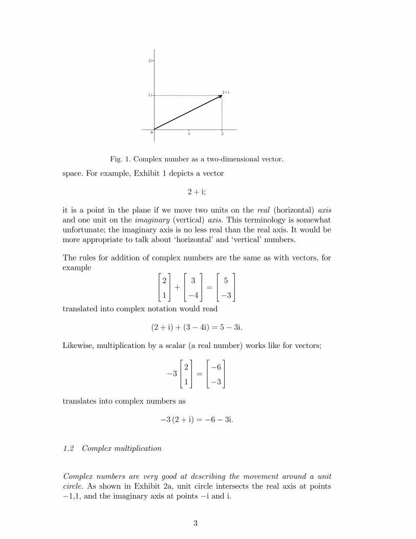
Fig. 1. Complex number as a two-dimensional vector.

space. For example, Exhibit 1 depicts a vector

2 + i;

it is a point in the plane if we move two units on the real (horizontal) axisand one unit on the imaginary (vertical) axis. This terminology is somewhatunfortunate; the imaginary axis is no less real than the real axis. It would bemore appropriate to talk about �horizontal�and �vertical�numbers.

The rules for addition of complex numbers are the same as with vectors, forexample 264 2

1

375+264 3

�4

375 =264 5

�3

375translated into complex notation would read

(2 + i) + (3� 4i) = 5� 3i:

Likewise, multiplication by a scalar (a real number) works like for vectors;

�3

264 21

375 =264�6�3

375translates into complex numbers as

�3 (2 + i) = �6� 3i:

1.2 Complex multiplication

Complex numbers are very good at describing the movement around a unitcircle. As shown in Exhibit 2a, unit circle intersects the real axis at points�1,1; and the imaginary axis at points �i and i.

3

10

ϕ

­i

­1

A

ia)

cos ϕ + i sin ϕ

i

10

ϕ

cos ϕ

i sin ϕ

b)

Fig. 2. Point on the unit circle expressed as a complex number.

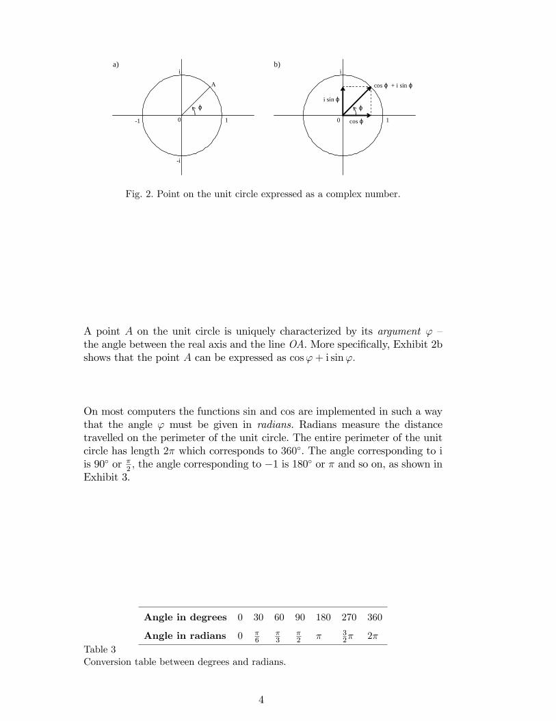
A point A on the unit circle is uniquely characterized by its argument ' �the angle between the real axis and the line OA. More speci�cally, Exhibit 2bshows that the point A can be expressed as cos'+ i sin':

On most computers the functions sin and cos are implemented in such a waythat the angle ' must be given in radians. Radians measure the distancetravelled on the perimeter of the unit circle. The entire perimeter of the unitcircle has length 2� which corresponds to 360�. The angle corresponding to iis 90� or �

2; the angle corresponding to �1 is 180� or � and so on, as shown in

Exhibit 3.

Angle in degrees 0 30 60 90 180 270 360

Angle in radians 0 �6

�3

�2 � 3

2� 2�

Table 3Conversion table between degrees and radians.

4

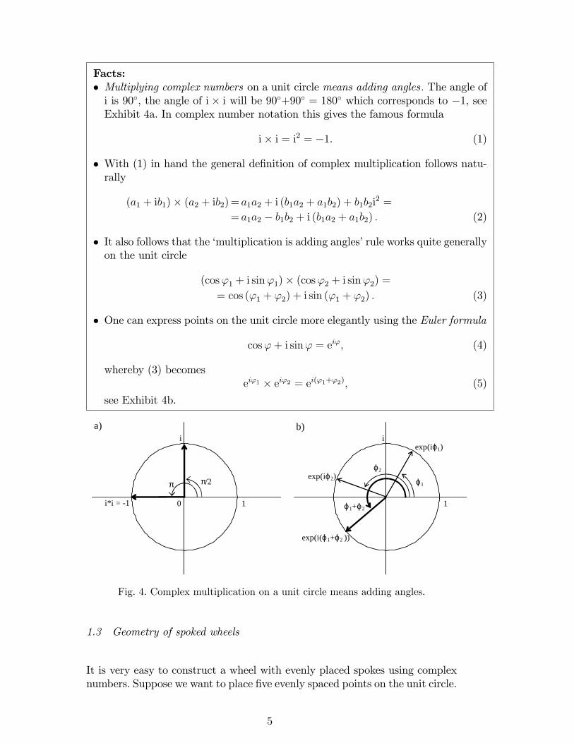
Facts:� Multiplying complex numbers on a unit circle means adding angles: The angle ofi is 90�; the angle of i � i will be 90�+90� = 180� which corresponds to �1; seeExhibit 4a. In complex number notation this gives the famous formula

i� i = i2 = �1: (1)

� With (1) in hand the general de�nition of complex multiplication follows natu-rally

(a1 + ib1)� (a2 + ib2)= a1a2 + i (b1a2 + a1b2) + b1b2i2 =

= a1a2 � b1b2 + i (b1a2 + a1b2) : (2)

� It also follows that the �multiplication is adding angles�rule works quite generallyon the unit circle

(cos'1 + i sin'1)� (cos'2 + i sin'2) == cos ('1 + '2) + i sin ('1 + '2) : (3)

� One can express points on the unit circle more elegantly using the Euler formula

cos'+ i sin' = ei'; (4)

whereby (3) becomesei'1 � ei'2 = ei('1+'2); (5)

see Exhibit 4b.

1

i

i*i = ­1

π

0

π/2

exp(i(ϕ1+ϕ2 ))

exp(iϕ2)

exp(iϕ1)

1

i

ϕ2

ϕ1

ϕ1+ϕ2

a) b)

Fig. 4. Complex multiplication on a unit circle means adding angles.

1.3 Geometry of spoked wheels

It is very easy to construct a wheel with evenly placed spokes using complexnumbers. Suppose we want to place �ve evenly spaced points on the unit circle.

5

One �fth of the full circle is characterized by the angle 2�5; hence the �rst spoke

will be placed at ei2�5 . Let us denote this number by z5 (�fth root of unity)

z5 � ei2�5 :

Since the multiplication by z5 causes anticlockwise rotation by one �fth of fullcircle the second spoke will be (z5)

2 the third spoke at (z5)3 and so on, see

Exhibit 5a.

4(z5)4

(z5)3

(z5)2

z5i

1 = (z5)0 = (z5)5

2π/5

­1

­41

2­3

­5 0 5

­23

a) b)

Fig. 5. a) Evenly distributed points on a circle. b) Number of elementary rotationsrequired to reach a particular spoke (+ anticlockwise, � clockwise).

This provides a natural numbering of the spokes, according to how manyelementary rotations are needed to reach the particular spoke. Note that sincewe are moving in a circle we will come back to the starting point after �verotations anticlockwise

(z5)0=(z5)

5 = (z5)10 = (z5)

15 = : : :

(z5)1=(z5)

6 = (z5)11 = (z5)

16 = : : : etc.,

and also after �ve rotations clockwise

(z5)0=(z5)

�5 = (z5)�10 = (z5)

�15 = : : :

(z5)1=(z5)

�4 = (z5)�9 = (z5)

�14 = : : : etc.

Thus the numbering of spokes is ambiguous; for example indices 0; 5;�5 referto the same spoke, see Exhibit 5b.

The following box summarizes the most important properties of evenly spacedpoints on the unit circle. These properties are essential for the understandingof the discrete Fourier transform.

6

� Let zn be a rotation by one nth of a full circle

zn � ei2�n :

Then(zn)

0 + (zn)1 + : : :+ (zn)

n�1 = 0 (6)

for any n. This is because the points (zn)0 ; (zn)

1 ; : : : ; (zn)n�1 are evenly distrib-

uted on a unit circle and thus the result of summation must not change if werotate the set of points by one nth of a full circle. The only vector that remainsunchanged after such rotation is zero vector.

� One can generalize this result further. Let k be an integer between 1 and n� 1.Then �

zkn�0+�zkn�1+ : : :+

�zkn�n�1

= 0 (7)

for any n. The reason for this result is again rotational symmetry of

points�zkn�0;�zkn�1; : : : ;

�zkn�n�1

. The di¤erence from (6) is that in the se-

quence (zn)0 ; (zn)

1 ; : : : ; (zn)n�1 each spoke occurs exactly once, whereas in�

zkn�0;�zkn�1; : : : ;

�zkn�n�1

the same spoke can occur several times (try n = 4;

k = 2).� The case with k = 0 requires special attention. Since (z0n)

j= 1 for all j we have�

zkn�0+�zkn�1+ : : :+

�zkn�n�1

= n:

To summarize,

�zkn�0+�zkn�1+ : : :+

�zkn�n�1

=n for k = 0;�n;�2n; : : : (8)�zkn�0+�zkn�1+ : : :+

�zkn�n�1

=0 for k 6= 0;�n;�2n; : : : (9)

1.4 Reverse order on a circle

Given a sequence of n numbers a = [a0; a1; : : : ; an�1] we can say that

rev(a) � [a0; an�1; : : : ; a1]

is a in reverse order. If a is written around a circle in anticlockwise directionthen rev(a) is found by reading from a0 in clockwise direction, see Exhibit 6.Note that rev(a) is not equal to [an�1; : : : ; a1; a0]:

7

an­1

a

rev(a )an­2

a1

a2

a0

Fig. 6. Reverse order on a circle.

For any k the sequence�zkn�0;�zkn�1; : : : ;

�zkn�n�1

is the same as the sequence�z�kn

�0;�z�kn

�1; : : : ;

�z�kn

�n�1taken in the reverse order:

rev��z�kn

�0;�z�kn

�1; : : : ;

�z�kn

�n�1�=�zkn�0;�zkn�1; : : : ;

�zkn�n�1

: (10)

This is because�z�kn

�n�j= z�kn+kjn = zkjn =

�zkn�jfor any j.

1.5 Discrete Fourier Transform (DFT)

As in the previous section take zn � ei2�n (this number is called the nth

root of unity ). Let a0; a1; : : : ; an�1 be a sequence of n (in general complex)numbers. The discrete Fourier transform of a0; a1; : : : ; an�1 is the sequenceb0; b1; : : : ; bn�1 such that

bk=a0�zkn�0+ a1

�zkn�1+ : : :+ an�1

�zkn�n�1

pn

= (11)

=1pn

n�1Xj=0

ajzjkn =

1pn

n�1Xj=0

ajei 2�njk

We writeF (a) = b:

Equation (11) represents the forward transform. The inverse transform is

~al=~b0�z�ln�0+~b1

�z�ln�1+ : : :+~bn�1

�z�ln�n�1

pn

= (12)

=1pn

n�1Xk=0

~bkz�kln =

1pn

n�1Xk=0

~bke�i 2�

nkl;

8

and we write

~a = F�1�~b�:

Facts:� The inverse discrete Fourier transform of sequence ~b0;~b1; : : : ;~bn�1 is the same asthe forward transform of the same sequence in reversed order

F�1�~b�= F

�rev

�~b��; (13)

and vice versaF�1

�rev

�~b��= F

�~b�: (14)

This is a direct consequence of (10).� F�1 is indeed an inverse transformation to F , that is

F�1 (F (a)) = F�F�1 (a)

�= a: (15)

This result relies on (8) and (9); for a proof see Appendix.

1.6 Binomial option pricing

Consider a monthly distribution of FTSE 100 return calibrated to re�ect mar-ket volatility of 4:4% a month and expected rate of return 0.9% a month:

pRu + (1� p)Rd=1:009

pR2u + (1� p)R2d=0:0442 + 1:0092:

Choosing the objective probability to be p = 12we solve for Ru and Rd

Ru=1: 053 with pu =1

2(16)

Rd=0: 965 with pd =1

2. (17)

Assuming that the initial value of FTSE Index is 5100.00 points, the evolutionof the index in the three months ahead is given by the lattice in Exhibit 7.

Suppose we wish to price a call option struck at K = 5355 (5% out of themoney), maturing 3 months from now. The intrinsic value of the option at

9

number of

low returnsS(0) S(1) S(2) S(3)

0 5100.00 5370.30 5654.93 5954.64

1 4921.50 5182.34 5457.00

2 4749.25 5000.96

3 4583.02Table 7Binomial stock price lattice.

maturity is

C(3) =

2666666664

599.64

102.00

0.00

0.00

3777777775: (18)

Asset pricing theory tells us that the no-arbitrage price of the pay-o¤264CuCd

375is given as the risk-neutral expectation of the discounted pay-o¤

no-arbitrage value(C) =quCu + qdCd

Rf; (19)

where the risk-neutral probabilities qu and qd are chosen such that the risk-neutrally expected return of all basis assets is equal to the risk-free return

qu + qd=1

quRu + qdRd=Rf :

The values qu=Rf and qd=Rf are known as state prices:

Assuming a risk-free rate equivalent to 4% per annum the monthly risk-freereturn is

Rf = 1:041=12 = 1:0033:

This gives conditional risk-neutral probabilities of

qu=Rf �RdRu �Rd

=1:0033� 0:9651:053� 0:965 = 0:43523; (20)

qd=Ru �RfRu �Rd

=1:053� 1:00331:053� 0:965 = 0:56477; (21)

10

and the valuation formula:

no-arbitrage value(C) =0:43523Cu + 0:56477Cd

1:0033: (22)

Recursive application of (22) with terminal value (18) leads to option pricesin Exhibit 8.

number of

low returnsC(0) C(1) C(2) C(3)

0 81.36 162.66 317.54 599.64

1 19.19 44.25 102.00

2 0.00 0.00

3 0.00Table 8Option prices in a binomial lattice.

1.7 Option pricing on a circle

For any two n-dimensional vectors a = [a0; a1; : : : ; an�1]; b = [b0; b1; : : : ; bn�1]we de�ne circular (cyclic) convolution of a and b to be a new vector c;

c = a~ b;

such that

cj =n�1Xk=0

aj�kbk: (23)

One will immediately note that the index j�k can be negative. If this occurs,we will simply add n to get the result between 0 and n � 1; this practice isconsistent with the spoke numbering introduced in Section 1.3, and it merelyre�ects movement in a circle.

Graphically one can evaluate the circular convolution as follows:

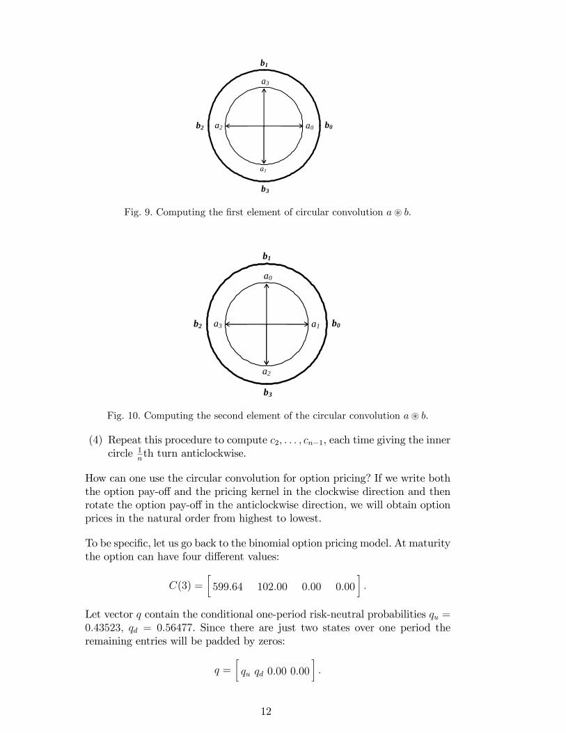
(1) Set up two concentric circles divided into n equal segments. Write aaround the inner circle clockwise and b around the outer circle anticlock-wise. Exhibit 9 shows this for n = 4:

(2) Perform a scalar multiplication between the two circles. In Exhibit 9 thiswould give

a0b0 + a3b1 + a2b2 + a1b3:

The result is c0:(3) Turn the inner circle anticlockwise by 1

nth of a full circle. Repeat the

scalar multiplication between the circles. The result is c1: In Exhibit 10

c1 = a1b0 + a0b1 + a3b2 + a2b3:

11

a0

a1

a2

a3

b3

b2

b1

b0

Fig. 9. Computing the �rst element of circular convolution a~ b:

a1

a2

a3

a0

b3

b2

b1

b0

Fig. 10. Computing the second element of the circular convolution a~ b.

(4) Repeat this procedure to compute c2; : : : ; cn�1, each time giving the innercircle 1

nth turn anticlockwise.

How can one use the circular convolution for option pricing? If we write boththe option pay-o¤ and the pricing kernel in the clockwise direction and thenrotate the option pay-o¤ in the anticlockwise direction, we will obtain optionprices in the natural order from highest to lowest.

To be speci�c, let us go back to the binomial option pricing model. At maturitythe option can have four di¤erent values:

C(3) =�599:64 102:00 0:00 0:00

�:

Let vector q contain the conditional one-period risk-neutral probabilities qu =0:43523; qd = 0:56477. Since there are just two states over one period theremaining entries will be padded by zeros:

q =�qu qd 0:00 0:00

�:

12

a)

599.64

0

102.00

0

0.5629

0000

0

0.4338

c)

0.5629

0000

0

0.4338599.64

102.00

0

0

d)

0.5629

0000

0

0.4338

599.64

102.00

0

0

b)

0.5629

0000

0

0.4338

599.64

102.00

0

0

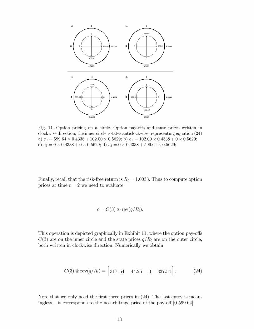
Fig. 11. Option pricing on a circle. Option pay-o¤s and state prices written inclockwise direction, the inner circle rotates anticlockwise, representing equation (24)a) c0 = 599:64� 0:4338 + 102:00� 0:5629; b) c1 = 102:00� 0:4338 + 0� 0:5629;c) c2 = 0� 0:4338 + 0� 0:5629; d) c3 =.0� 0:4338 + 599:64� 0:5629;

Finally, recall that the risk-free return is Rf = 1:0033. Thus to compute optionprices at time t = 2 we need to evaluate

c = C(3)~ rev(q=Rf):

This operation is depicted graphically in Exhibit 11, where the option pay-o¤sC(3) are on the inner circle and the state prices q=Rf are on the outer circle,both written in clockwise direction. Numerically we obtain

C(3)~ rev(q=Rf) =�317: 54 44:25 0 337:54

�: (24)

Note that we only need the �rst three prices in (24). The last entry is mean-ingless �it corresponds to the no-arbitrage price of the pay-o¤ [0 599.64].

13

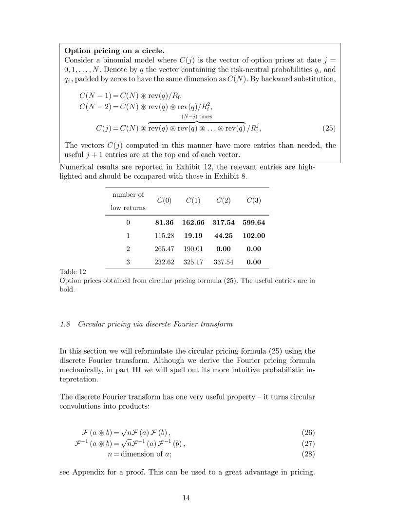
Option pricing on a circle.Consider a binomial model where C(j) is the vector of option prices at date j =0; 1; : : : ; N . Denote by q the vector containing the risk-neutral probabilities qu andqd, padded by zeros to have the same dimension as C(N): By backward substitution,

C(N � 1)=C(N)~ rev(q)=Rf;C(N � 2)=C(N)~ rev(q)~ rev(q)=R2f ;

C(j)=C(N)~(N�j) timesz }| {

rev(q)~ rev(q)~ : : :~ rev(q) =Rjf ; (25)

The vectors C(j) computed in this manner have more entries than needed, theuseful j + 1 entries are at the top end of each vector.

Numerical results are reported in Exhibit 12, the relevant entries are high-lighted and should be compared with those in Exhibit 8.

number of

low returnsC(0) C(1) C(2) C(3)

0 81.36 162.66 317.54 599.64

1 115.28 19.19 44.25 102.00

2 265.47 190.01 0.00 0.00

3 232.62 325.17 337.54 0.00Table 12Option prices obtained from circular pricing formula (25). The useful entries are inbold.

1.8 Circular pricing via discrete Fourier transform

In this section we will reformulate the circular pricing formula (25) using thediscrete Fourier transform. Although we derive the Fourier pricing formulamechanically, in part III we will spell out its more intuitive probabilistic in-tepretation.

The discrete Fourier transform has one very useful property �it turns circularconvolutions into products:

F (a~ b)=pnF (a)F (b) ; (26)

F�1 (a~ b)=pnF�1 (a)F�1 (b) ; (27)

n=dimension of a; (28)

see Appendix for a proof. This can be used to a great advantage in pricing.

14

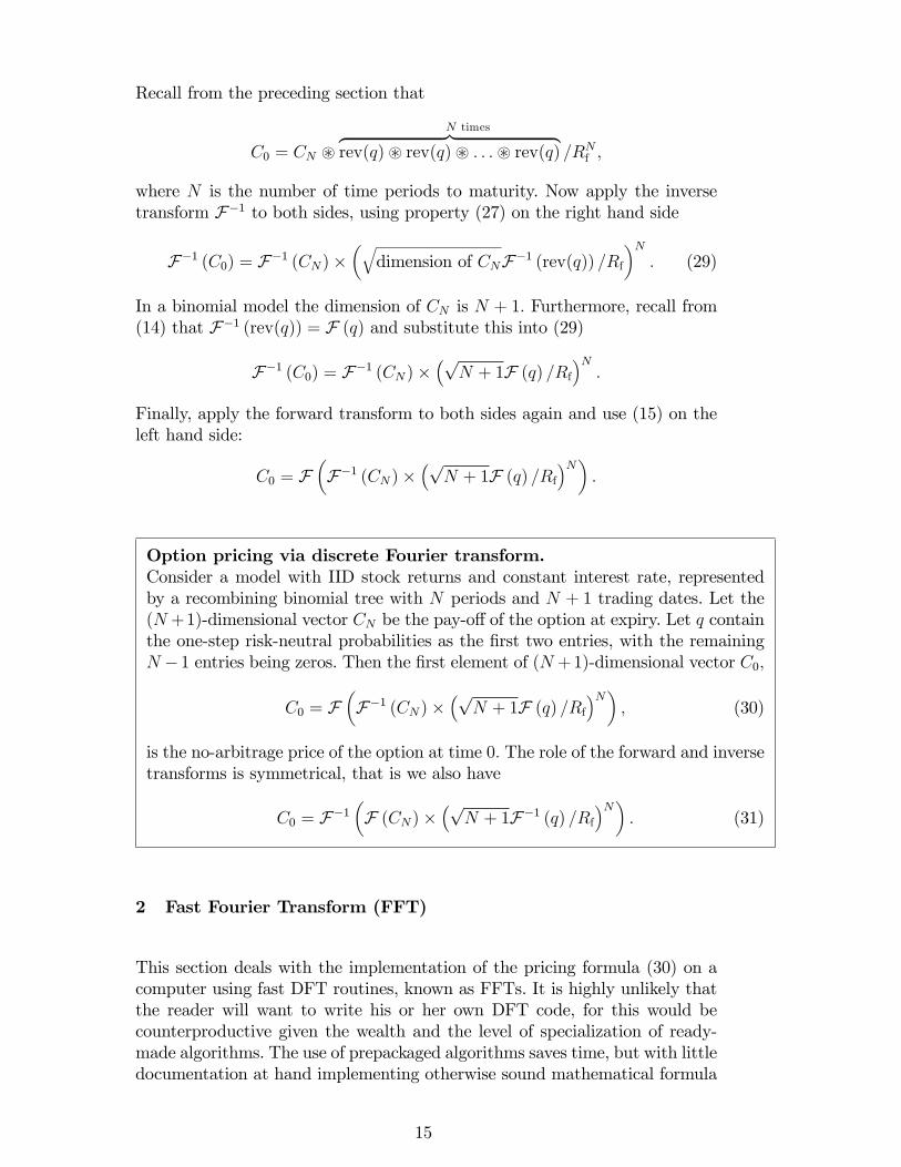
Recall from the preceding section that

C0 = CN ~N timesz }| {

rev(q)~ rev(q)~ : : :~ rev(q) =RNf ;

where N is the number of time periods to maturity. Now apply the inversetransform F�1 to both sides, using property (27) on the right hand side

F�1 (C0) = F�1 (CN)��qdimension of CNF�1 (rev(q)) =Rf

�N: (29)

In a binomial model the dimension of CN is N + 1: Furthermore, recall from(14) that F�1 (rev(q)) = F (q) and substitute this into (29)

F�1 (C0) = F�1 (CN)��p

N + 1F (q) =Rf�N

:

Finally, apply the forward transform to both sides again and use (15) on theleft hand side:

C0 = F�F�1 (CN)�

�pN + 1F (q) =Rf

�N�:

Option pricing via discrete Fourier transform.Consider a model with IID stock returns and constant interest rate, representedby a recombining binomial tree with N periods and N + 1 trading dates. Let the(N +1)-dimensional vector CN be the pay-o¤ of the option at expiry. Let q containthe one-step risk-neutral probabilities as the �rst two entries, with the remainingN �1 entries being zeros. Then the �rst element of (N +1)-dimensional vector C0;

C0 = F�F�1 (CN)�

�pN + 1F (q) =Rf

�N�; (30)

is the no-arbitrage price of the option at time 0: The role of the forward and inversetransforms is symmetrical, that is we also have

C0 = F�1�F (CN)�

�pN + 1F�1 (q) =Rf

�N�: (31)

2 Fast Fourier Transform (FFT)

This section deals with the implementation of the pricing formula (30) on acomputer using fast DFT routines, known as FFTs. It is highly unlikely thatthe reader will want to write his or her own DFT code, for this would becounterproductive given the wealth and the level of specialization of ready-made algorithms. The use of prepackaged algorithms saves time, but with littledocumentation at hand implementing otherwise sound mathematical formula

15

may not prove straightforward. This section provides guidelines that ensurea trouble-free transition between the theoretical pricing formula (30) and acomputer code using a DFT routine of reader�s choice, with speci�c examplesgiven in GAUSS and MATLAB.

Two main issues arise in the use of (fast) DFT routines: 1) �nding out themathematical de�nition of a speci�c DFT routine, and 2) choosing the rightinput length to make the computation fast. We now address these two issuesin turn.

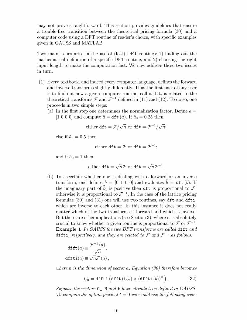
(1) Every textbook, and indeed every computer language, de�nes the forwardand inverse transforms slightly di¤erently. Thus the �rst task of any useris to �nd out how a given computer routine, call it dft, is related to thetheoretical transforms F and F�1 de�ned in (11) and (12). To do so, oneproceeds in two simple steps:(a) In the �rst step one determines the normalization factor. De�ne a =

[1 0 0 0] and compute ~a = dft (a). If ~a0 = 0:25 then

either dft = F=pn or dft = F�1=

pn;

else if ~a0 = 0:5 then

either dft = F or dft = F�1;

and if ~a0 = 1 then

either dft =pnF or dft =

pnF�1:

(b) To ascertain whether one is dealing with a forward or an inversetransform, one de�nes b = [0 1 0 0] and evaluates ~b = dft (b). Ifthe imaginary part of ~b1 is positive then dft is proportional to F ;otherwise it is proportional to F�1. In the case of the lattice pricingformulae (30) and (31) one will use two routines, say dft and dfti,which are inverse to each other. In this instance it does not reallymatter which of the two transforms is forward and which is inverse.But there are other applications (see Section 3), where it is absolutelycrucial to know whether a given routine is proportional to F or F�1.Example 1 In GAUSS the two DFT transforms are called dfft anddffti, respectively, and they are related to F and F�1 as follows:

dfft(a)� F�1 (a)pn

;

dffti(a)�pnF (a) ;

where n is the dimension of vector a. Equation (30) therefore becomes

C0 = dffti�dfft (CN)� (dffti (b))N

�: (32)

Suppose the vectors C_ N and b have already been de�ned in GAUSS.To compute the option price at t = 0 we would use the following code:

16

C_0 = dffti( dfft(C_N).*(dfft(b)^N) ); (33)print ��no-arbitrage price at t=0 is �� C_0[1];

The �:��command stands for element-by-element multiplication.The DFT algorithm is approximately three times faster than the

backward recursion in binomial model; the computational time forboth algorithms grows quadratically with the number of periods 1 ,see Exhibit 13.

trading interval number of execution time in seconds

in minutes periods DFT backward recursion

60 504 0.15 0.4

30 1008 0.6 1.6

15 2016 2.3 6.4

5 6048 20.8 61.6

Pentium III 750MHz, 128Mb RAM, GAUSSTable 13Comparison of pricing speed in a binomial lattice between backward recursion anddiscrete Fourier transform formula (30).

(2) A naive implementation of DFT algorithm with n-dimensional input re-quires n2 complex multiplications (see example above). An e¢ cient im-plementation of DFT, known as the fast Fourier transform (FFT), willonly require Kn lnn operations 2 , but one still has to choose n carefullybecause the constant K can be very large for some choices of n. SomeFFT implementations automatically restrict the transform length to themost suitable values of n (typically n = 2p or n = 2p3q5r); which is thecase in GAUSS. Others, such as MATLAB, will compute FFT of anylength; here it is particularly important for the user to choose n sensibly,otherwise the FFT algorithm may turn out to be very slow indeed.Example 2 The forward and inverse FFT in MATLAB are called fftand ifft, respectively:

fft(a)�pnF�1 (a) (34)

ifft(a)� F (a)pn; (35)

1 GAUSS programes Binomial.gss and DFT.gss available from author�s website.2 The fast Fourier transform does not appear in undergraduate textbooks on nu-merical mathematics and the most useful references on the introductory level areweb based, see http://www.fftw.org/links.html, and in particular the onlinemanual Hey [1999]. An e¢ cient implementation of FFT for all transform lengths issuggested in Frigo and Johnson [1998]; it is used in Matlab. E¢ cient implementationof mixed 2; 3; 5-radix algorithm is due to Temperton [1992]; it is used in GAUSS.Duhamel and Vetterli [1990] is an excellent survey of FFT algorithms.

17

where n is the dimension of vector a. The option pricing equation (30)therefore becomes

C0 = ifft�fft (CN)� ((N + 1)� ifft (b))N

�;

which in terms of MATLAB code reads

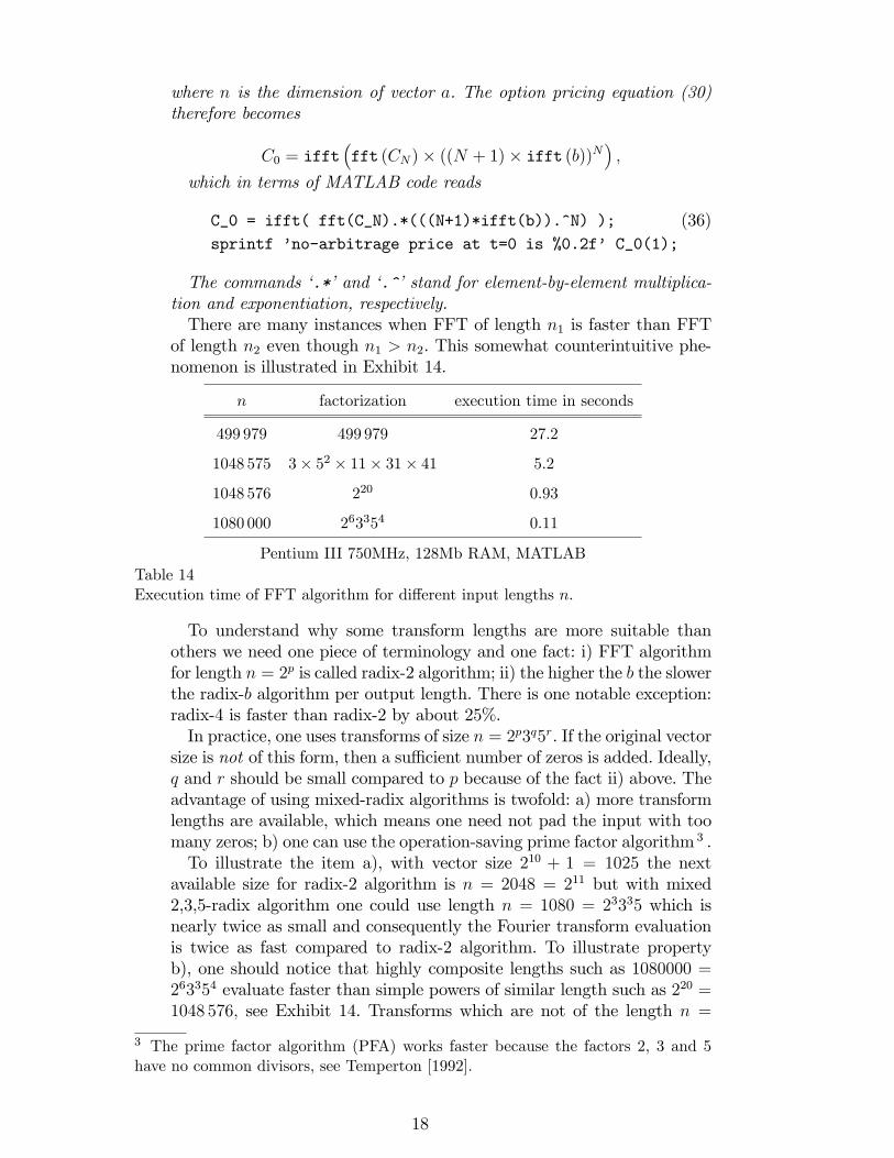
C_0 = ifft( fft(C_N).*(((N+1)*ifft(b)).^N) ); (36)sprintf �no-arbitrage price at t=0 is %0.2f� C_0(1);

The commands �.*�and �.^�stand for element-by-element multiplica-tion and exponentiation, respectively.There are many instances when FFT of length n1 is faster than FFT

of length n2 even though n1 > n2. This somewhat counterintuitive phe-nomenon is illustrated in Exhibit 14.

n factorization execution time in seconds

499 979 499 979 27.2

1048 575 3� 52 � 11� 31� 41 5.2

1048 576 220 0.93

1080 000 263354 0.11

Pentium III 750MHz, 128Mb RAM, MATLABTable 14Execution time of FFT algorithm for di¤erent input lengths n.

To understand why some transform lengths are more suitable thanothers we need one piece of terminology and one fact: i) FFT algorithmfor length n = 2p is called radix-2 algorithm; ii) the higher the b the slowerthe radix-b algorithm per output length. There is one notable exception:radix-4 is faster than radix-2 by about 25%.In practice, one uses transforms of size n = 2p3q5r. If the original vector

size is not of this form, then a su¢ cient number of zeros is added. Ideally,q and r should be small compared to p because of the fact ii) above. Theadvantage of using mixed-radix algorithms is twofold: a) more transformlengths are available, which means one need not pad the input with toomany zeros; b) one can use the operation-saving prime factor algorithm 3 .To illustrate the item a), with vector size 210 + 1 = 1025 the next

available size for radix-2 algorithm is n = 2048 = 211 but with mixed2,3,5-radix algorithm one could use length n = 1080 = 23335 which isnearly twice as small and consequently the Fourier transform evaluationis twice as fast compared to radix-2 algorithm. To illustrate propertyb), one should notice that highly composite lengths such as 1080000 =263354 evaluate faster than simple powers of similar length such as 220 =1048 576; see Exhibit 14. Transforms which are not of the length n =

3 The prime factor algorithm (PFA) works faster because the factors 2, 3 and 5have no common divisors, see Temperton [1992].

18

2p3q5r can take very long to compute, especially if n is a large prime,again see Exhibit 14.Example 3 MATLAB will allow the user to perform FFT of any length;this is done using commands (34) and (35). However, as we have notedabove, it is eminently sensible to restrict transform lengths to n = 2p3q5r

with q and r small relative to p to obtain the best performance. MAT-LAB provides function nextpow2 giving the next bigger power of 2. Inaddition, MATLAB allows the user to specify the transform length by in-cluding it as a second optional argument of fft and ifft. Hence a fastimplementation of (36) in MATLAB would read:

length = 2^nextpow2(N+1);

C_0 = ifft( fft(C_N,length).*((length*ifft(b,length)).^N) );

The padding of the original input C_N by zeros to the dimension lengthis done automatically.To �nd the nearest transform length of the form n = 2p3q5r one can

use the following code:

length = N+1;

while max(factor(length)) > 5;

length = length+1;

end;

Example 4 In GAUSS the fast Fourier forward and inverse transformsare performed by functions fftn and ffti. These functions use Temper-ton�s [1992] mixed 2,3,5-radix algorithm, and the padding of input vectorby zeros to the nearest available length n = 2p3q5r is done automatically.If n is the input dimension the output dimension from fftn and ffti willbe nextn(n). In terms of GAUSS code one writes similarly as in (33):

C_0 = ffti( fftn(C_N).*(ffti(b)^N) );

One can increase the speed further by choosing a composite length n =2p3q5r where q and r are non-zero but small relative to p: The optimallength is given by GAUSS function optn (N + 1) ; and the padding byzeros to this dimension must be performed by the user.

The FFT implementation of binomial pricing algorithm 4 has a blisteringspeed compared to the DFT, see Exhibit 15.

Because it is so fast one can explore higher trading frequencies and see thatthe Black�Scholes formula really does describe the limiting value, see Exhibit16. Note that the Black�Scholes formula itself is still about 10 000 times fasterthan the FFT algorithm.

4 GAUSS code FFT.gss available from author�s website.

19

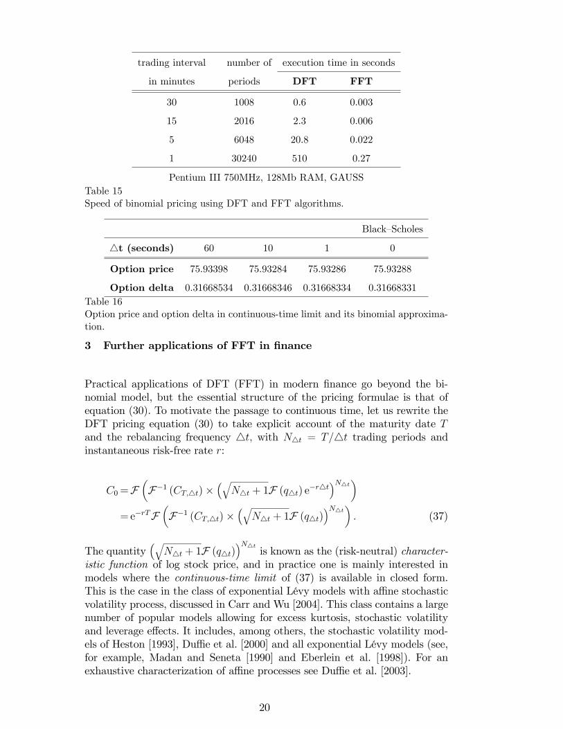
trading interval number of execution time in seconds

in minutes periods DFT FFT

30 1008 0.6 0.003

15 2016 2.3 0.006

5 6048 20.8 0.022

1 30240 510 0.27

Pentium III 750MHz, 128Mb RAM, GAUSSTable 15Speed of binomial pricing using DFT and FFT algorithms.

Black�Scholes

4t (seconds) 60 10 1 0

Option price 75.93398 75.93284 75.93286 75.93288

Option delta 0.31668534 0.31668346 0.31668334 0.31668331Table 16Option price and option delta in continuous-time limit and its binomial approxima-tion.

3 Further applications of FFT in �nance

Practical applications of DFT (FFT) in modern �nance go beyond the bi-nomial model, but the essential structure of the pricing formulae is that ofequation (30). To motivate the passage to continuous time, let us rewrite theDFT pricing equation (30) to take explicit account of the maturity date Tand the rebalancing frequency 4t; with N4t = T=4t trading periods andinstantaneous risk-free rate r:

C0=F�F�1 (CT;4t)�

�qN4t + 1F (q4t) e�r4t

�N4t�=e�rTF

�F�1 (CT;4t)�

�qN4t + 1F (q4t)

�N4t�: (37)

The quantity�q

N4t + 1F (q4t)�N4t

is known as the (risk-neutral) character-istic function of log stock price, and in practice one is mainly interested inmodels where the continuous-time limit of (37) is available in closed form.This is the case in the class of exponential Lévy models with a¢ ne stochasticvolatility process, discussed in Carr and Wu [2004]. This class contains a largenumber of popular models allowing for excess kurtosis, stochastic volatilityand leverage e¤ects. It includes, among others, the stochastic volatility mod-els of Heston [1993], Du¢ e et al. [2000] and all exponential Lévy models (see,for example, Madan and Seneta [1990] and Eberlein et al. [1998]). For anexhaustive characterization of a¢ ne processes see Du¢ e et al. [2003].

20

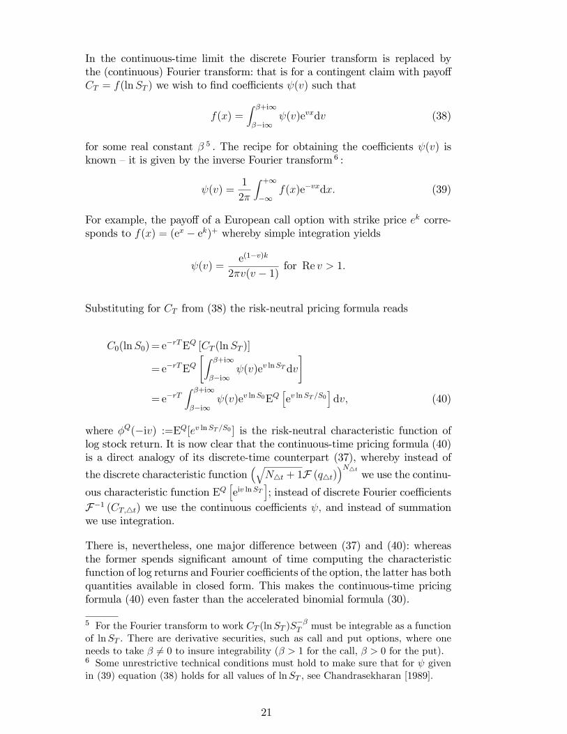
In the continuous-time limit the discrete Fourier transform is replaced bythe (continuous) Fourier transform: that is for a contingent claim with payo¤CT = f(lnST ) we wish to �nd coe¢ cients (v) such that

f(x) =Z �+i1

��i1 (v)evxdv (38)

for some real constant � 5 . The recipe for obtaining the coe¢ cients (v) isknown �it is given by the inverse Fourier transform 6 :

(v) =1

2�

Z +1

�1f(x)e�vxdx: (39)

For example, the payo¤ of a European call option with strike price ek corre-sponds to f(x) = (ex � ek)+ whereby simple integration yields

(v) =e(1�v)k

2�v(v � 1) for Re v > 1:

Substituting for CT from (38) the risk-neutral pricing formula reads

C0(lnS0)= e�rTEQ [CT (lnST )]

= e�rTEQ"Z �+i1

��i1 (v)ev lnST dv

#

=e�rTZ �+i1

��i1 (v)ev lnS0EQ

hev lnST =S0

idv; (40)

where �Q(�iv) :=EQ[ev lnST =S0 ] is the risk-neutral characteristic function oflog stock return. It is now clear that the continuous-time pricing formula (40)is a direct analogy of its discrete-time counterpart (37), whereby instead of

the discrete characteristic function�q

N4t + 1F (q4t)�N4t

we use the continu-

ous characteristic function EQheiv lnST

i; instead of discrete Fourier coe¢ cients

F�1 (CT;4t) we use the continuous coe¢ cients ; and instead of summationwe use integration.

There is, nevertheless, one major di¤erence between (37) and (40): whereasthe former spends signi�cant amount of time computing the characteristicfunction of log returns and Fourier coe¢ cients of the option, the latter has bothquantities available in closed form. This makes the continuous-time pricingformula (40) even faster than the accelerated binomial formula (30).

5 For the Fourier transform to work CT (lnST )S��T must be integrable as a function

of lnST : There are derivative securities, such as call and put options, where oneneeds to take � 6= 0 to insure integrability (� > 1 for the call, � > 0 for the put).6 Some unrestrictive technical conditions must hold to make sure that for givenin (39) equation (38) holds for all values of lnST , see Chandrasekharan [1989].

21

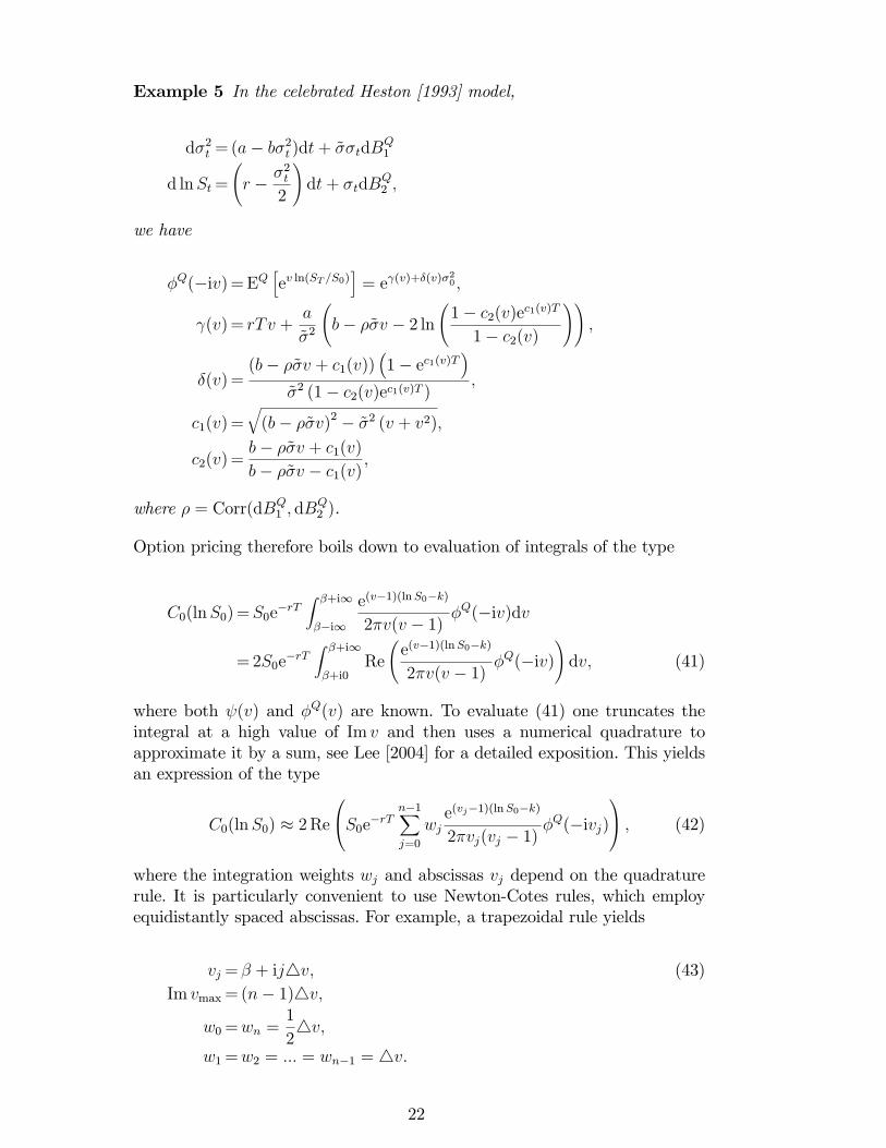
Example 5 In the celebrated Heston [1993] model,

d�2t =(a� b�2t )dt+ ~��tdBQ1

d lnSt=

r � �2t

2

!dt+ �tdB

Q2 ;

we have

�Q(�iv)=EQhev ln(ST =S0)

i= e (v)+�(v)�

20 ;

(v)= rTv +a

~�2

b� �~�v � 2 ln

1� c2(v)e

c1(v)T

1� c2(v)

!!;

�(v)=(b� �~�v + c1(v))

�1� ec1(v)T

�~�2 (1� c2(v)ec1(v)T )

;

c1(v)=q(b� �~�v)2 � ~�2 (v + v2);

c2(v)=b� �~�v + c1(v)

b� �~�v � c1(v);

where � = Corr(dBQ1 ; dB

Q2 ).

Option pricing therefore boils down to evaluation of integrals of the type

C0(lnS0)=S0e�rT

Z �+i1

��i1

e(v�1)(lnS0�k)

2�v(v � 1) �Q(�iv)dv

=2S0e�rT

Z �+i1

�+i0Re

e(v�1)(lnS0�k)

2�v(v � 1) �Q(�iv)

!dv; (41)

where both (v) and �Q(v) are known. To evaluate (41) one truncates theintegral at a high value of Im v and then uses a numerical quadrature toapproximate it by a sum, see Lee [2004] for a detailed exposition. This yieldsan expression of the type

C0(lnS0) � 2Re0@S0e�rT n�1X

j=0

wje(vj�1)(lnS0�k)

2�vj(vj � 1)�Q(�ivj)

1A ; (42)

where the integration weights wj and abscissas vj depend on the quadraturerule. It is particularly convenient to use Newton-Cotes rules, which employequidistantly spaced abscissas. For example, a trapezoidal rule yields

vj = � + ij4v; (43)Im vmax=(n� 1)4v;

w0=wn =1

24v;

w1=w2 = ::: = wn�1 = 4v:

22

In conclusion, if the characteristic function of log returns is known, one needsto evaluate a single sum (42) to �nd the option price. Consequently, there isno need to use FFT if one wishes to evaluate the option price for one �xedlog strike k.

3.1 FFT option pricing with multiple strikes

The situation is very di¤erent if we want to evaluate the option price (42)for many di¤erent strikes simultaneously. Let us consider m = 121 valuesof moneyness �l = lnS0 � kl ranging from �30% to 30% with increment4� = 0:5%

�l=�max � l4�; (44)�max=0:30; l = 0; : : : ;m� 1: (45)

The idea of using FFT in this context is due to Carr and Madan [1999],and it has recently been improved upon by using so-called z-transform, seeChourdakis [2004]:

De�nition 6 The number

a0z0 + a1z

�1 + : : :+ an�1z�(n�1)

is called the z-transform of sequence a: The discrete Fourier transform ofsequence a is obtained as a special case of z-transform with n speci�c valuesof z:

zl = e�i 2�

nl; l = 0; 1; : : : ; n� 1.

Carr and Madan have noted that with equidistantly spaced abscissas (43) onecan write the option pricing equation (42) for di¤erent strike values (44, 45)as a z-transform with zl = e�i4v4�l:

C0l=2S0e(��1)�l�rT Re

n�1Xk=0

ei4v4�klaj; (46)

aj =wjeij4v�max�Q(�ivj)2�vj(vj � 1)

:

Setting

4v4� = 2�

n(47)

Carr and Madan obtain a discrete Fourier transform in (46). Chourdakis [2004]points out that there is a fast algorithm for the z-transform which works evenwhen 4v4� 6= 2�

nand m 6= n:

23

Chirp-z transformChirp-z transform is an e¢ cient algorithm for evaluating the z-transform for mdi¤erent points z of the form

zk = Awk; k = 0; 1; : : : ;m� 1;

where A and w are arbitrary complex numbers. The chirp-z transform works byrephrasing the original z-transform as a circular convolution and then computingthis convolution by means of three FFTs as shown in Part I, Section �Circularpricing via DFT�. For more details see Bluestein [1968], Rabiner et al. [1969], andBailey and Swartztrauber [1991]. Compared to the standard n-long FFT the chirp-zalgorithm is approximately 6(lnm+ 1)= lnn times slower, for m � n:The MATLAB command for chirp-z transform of n-long input sequence a reads

czt(a;m;w;A).

A GAUSS procedure czt.gss is available from author�s website.

The decision whether to use the simple summation (42) m times, or whetherto apply the chirp-z transform (46) depends on the desired number of strikesm. The speed of the former relative to the latter is roughly m=6=(log2m+ 1)times higher. As a rough guide, for m � 36 the simple summation (42) is asfast as the chirp-z formula (46), for m = 8 it is three times faster, and form = 150 it is three times slower.

One also has to decide whether to force the FFT spacing of strike values (47);this is done by boosting n while keeping4v �xed. Suppose that vmax is chosensu¢ ciently high to achieve desired accuracy for a single strike. As a rule ofthumb, if the initial spacing 2�

Im vmaxis six times coarser that the desired spacing

of log strikes 4� one should use the chirp-z transform, otherwise it will befaster to increase n to satisfy (47) and use the short FFT algorithm describedin Bailey and Schwarztrauber [2004, pp. 392-393].

The value of Im vmax tends to be higher for short maturities, and for para-metric distributions with heavy tails, such as variance gamma or generalizedhyperbolic. In such circumstances FFT formula (46)-(47) is preferable. Non-parametric empirical equity return distributions have characterisitic functionsthat decay faster, leading to lower values of Im vmax, leaving the chirp-z trans-form as the best option.

4 Conclusions

The present paper makes three contributions. It explains the working of thediscrete Fourier transform in a non-technical language in the familiar bino-

24

mial option pricing model. Secondly, it highlights the common perils in thecomputer implementation of fast DFT algorithms. Thirdly, it explains howthe binomial pricing formula relates to more complex continuous-time modelswhich allow for excess kurtosis, stochastic volatility and leverage e¤ects andwhich are used routinely in the �nance industry.

The present paper does not give an exhaustive account of DFT in Finance.One can quite easily extend the Fourier pricing formula from binomial lat-tice of Part I to multinomial lattices, see µCerný [2004, Chapter 12]. Furtherapplications of FFT appear in Albanese et al [2004], Andreas et al. [2002], Ben-hamou [2002], Chiarella and El-Hassan [1997], Dempster and Hong [2002], andRebonato and Cooper [1998]. For the most up-to-date developments in optionpricing using (continuous) Fourier transform see Carr and Wu [2004], and forevalution of hedging errors refer to µCerný [2003] and Hubalek et al [2004].

Notes

I would like to thank David Miles and Jonathan Wainwright for suggesting im-portant clari�cations in an early draft. I am grateful to Peter Carr, Sanjiv Dasand Stephen Figlewski, who provided helpful comments and pointers to references.This is an abridged and adapted version of of µCerný [2004, Chapter 7]. GAUSS isa trademark of Aptech Systems, Inc.; MATLAB is a registered trademark of TheMathWorks, Inc.

5 Appendix

5.1 Inverse Discrete Fourier Transform

To show F�1 (F (a)) = a we need to prove that for b = F (a) de�ned in (11)we have F�1 (b) = a: Denote ~a = F�1 (b) and express ~a from de�nition (12)

~al =1pn

n�1Xk=0

bkz�kln :

Now substitute for bk from (11)

~al =1

n

n�1Xk=0

0@n�1Xj=0

ajzjkn

1A z�kln ;

25

move z�kln inside the inner summation

~al =1

n

n�1Xk=0

0@n�1Xj=0

ajzk(j�l)n

1A ;change the order of summation

~al =1

n

n�1Xj=0

n�1Xk=0

ajzk(j�l)n

!;

and take aj in front of the inner sum (it does not depend on k)

~al =1

n

n�1Xj=0

aj

n�1Xk=0

�zj�ln

�k!:

By virtue of (8)-(9) the inner sumPn�1k=0

�zj�ln

�kequals 0 for j 6= l and for

j = l it equals n. Consequently

~al =1

n

n�1Xj=0

aj

n�1Xk=0

�zj�ln

�k!= al

for all l which proves that F�1 (F (a)) = a:

5.2 Discrete Fourier Transform of Convolutions

We wish to show F(a~b) = pnF(a)F(b): Let us begin by computing c = a~b:From the de�nition (23)

cj =n�1Xk=0

aj�kbk: (48)

By d denote the Fourier transform of c; d = F(a ~ b) and use the de�nition(11) to evaluate dl

dl =1pn

n�1Xj=0

cjzjln :

Now substitute for cj from (48),

dl =1pn

n�1Xj=0

n�1Xk=0

aj�kbk

!zjln ;

move zjl inside the inner bracket, writing it as a product zjl = z(j�k)lzkl;

dl =1pn

n�1Xj=0

n�1Xk=0

aj�kz(j�k)lbkz

kl;

26

change the order of summation,

dl =1pn

n�1Xk=0

n�1Xj=0

aj�kz(j�k)lbkz

kl;

and take bkzkl in front of the inner summation (it does not depend on j),

dl =1pn

n�1Xk=0

bkzkl

0@n�1Xj=0

aj�kz(j�k)l

1A : (49)

It is easy to realize that the inner sum does not depend on k, because it alwaysadds the same n elements; only the order in which these elements are addeddepends on k (we are completing one full turn around the circle, starting atkth spoke). Hence we have:

n�1Xj=0

aj�kz(j�k)l =

n�1Xj=0

ajzjl for all k;

and substituting this into (49) we �nally obtain

dl =pn

1pn

n�1Xk=0

bkzkl

!| {z }

~bl

0@ 1pn

n�1Xj=0

ajzjl

1A| {z }

~al

:

From the de�nition of the forward transform (11) ~a = F(a) and ~b = F(b);which completes the proof.

27

References

Albanese, C., Jackson, K., and Wiberg, P. A new Fourier transform algo-rithm for value at risk. Quantitative Finance 4 (2004), 328�338.

Andreas, A., Engelmann, B., Schwendner, P., and Wystup, U. Fast Fouriermethod for the valuation of options on several correlated currencies. InForeign Exchange Risk, J. Hakala and U. Wystup, Eds. Risk Publications,2002.

Bailey, D. H., and Swartztrauber, P. N. The fractional Fourier transformand applications. SIAM Review 33, 3 (1991), 389�404.

Benhamou, E. Fast Fourier transform for discrete Asian options. Journalof Computational Finance 6, 1 (2002).

Bluestein, L. I. A linear �ltering approach to the computation of the discreteFourier transform. IEEE Northeast Electronics Research and EngineeringMeeting 10 (1968), 218�219.

Carr, P., and Madan, D. B. Option valuation using the fast Fourier trans-form. Journal of Computational Finance 2 (1999), 61�73.

Carr, P., and Wu, L. Time-changed Lévy processes and option pricing.Journal of Financial Economics 71, 1 (2004), 113�141.

µCerný, A. The risk of optimal, continuously rebalanced hedging strategiesand its e¢ cient evaluation via Fourier transform. Tech. rep., The BusinessSchool, Imperial College London, 2003.

µCerný, A. Mathematical Techniques in Finance: Tools for Incomplete Mar-kets. Princeton University Press, 2004.

Chandrasekharan, K. Classical Fourier Transforms. Springer, 1989.

Chiarella, C., and El-Hassan, N. Evaluation of derivative security pricesin the heath-jarrow-morton framework as path integrals using fast Fouriertransform techniques. Journal of Financial Engineering 6, 2 (1997), 121�147.

Chourdakis, K. Option pricing using the fractional FFT. Working paper onwww.theponytail.net, 2004.

Dempster, M. A. H., and Hong, S. S. G. Spread option valuation andthe fast Fourier transform. In Mathematical Finance �Bachelier Congress2000, H. Geman, D. Madan, S. R. Pliska, and T. Vorst, Eds. Springer, 2002,pp. 203�220.

Du¢ e, D., Filipovic, D., and Schachermayer, W. A¢ ne processes and appli-cations in �nance. The Annals of Applied Probability 13, 3 (2003), 984�1053.

Du¢ e, D., Pan, J., and Singleton, K. Transform analysis and asset pricingfor a¢ ne jump di¤usions. Econometrica 68 (2000), 1343�1376.

28

Duhamel, P., and Vetterli, M. Fast Fourier transforms: A tutorial reviewand a state of the art. Signal Processing 19 (1990), 259�299.

Eberlein, E., Keller, U., and Prause, K. New insights into smile, mispricingand value at risk: The hyperbolic model. Journal of Business 71, 3 (1998),371�405.

Frigo, M., and Johnson, S. G. FFTW: An adaptive software architecturefor the FFT. In Proc. IEEE Intl. Conf. On Acoustics, Speech, and SignalProcessing (Seattle, WA, 1998), vol. 3, pp. 1381�1384.

Heston, S. A closed-form solution for options with stochastic volatility withapplications to bond and currency options. Review of Financial Studies 6(1993), 327�344.

Hey, A. FFT Demysti�ed. http://www.eptools.com/tn/T0001/INDEX.HTM,1999.

Hubalek, F., Kallsen, J., and Krawczyk, L. Variance-optimal hedging andMarkowitz-e¢ cient portfolios for processes with stationary independent in-crements. Working paper, 2004.

Lee, R. W. Option pricing by transform methods: Extensions, uni�cationand error control. Journal of Computational Finance 7, 3 (2004).

Madan, D., and Seneta, E. The variance gamma model for stock marketreturns. Journal of Business 63, 4 (1990), 511�524.

Rabiner, L. R., Schafer, R. W., and Rader, C. M. The chirp z-transformalgorithm and its application. Bell Systems Technical Journal 48, 5 (1969),1249�1292.

Rebonato, R., and Cooper, I. Coupling backward induction with montecarlo simulations: A fast Fourier transform (FFT) approach. Applied Math-ematical Finance 5, 2 (1998), 131�141.

Temperton, C. A generalized prime factor FFT algorithm for any n = 2p3q5s.SIAM Journal on Scienti�c and Statistical Computing 13 (1992), 676�686.

29