Fast forecast reconciliation using linear models

Department of Econometrics and Business Statistics

http://monash.edu/business/ebs/research/publications

Fast forecast reconciliation

using linear models

Mahsa Ashouri, Rob J Hyndman, Galit Shmueli

December 2019

Working Paper 29/19

ISSN 1440-771X

Fast forecast reconciliation using

linear models

Mahsa AshouriInstitute of Service Science, National Tsing Hua University, TaiwanEmail: [email protected] author

Rob J HyndmanMonash University, Clayton VIC 3800, AustraliaEmail: [email protected]

Galit ShmueliInstitute of Service Science, National Tsing Hua University, TaiwanEmail: [email protected]

3 December 2019

JEL classification: C10,C14,C22

mailto:[email protected]



Fast forecast reconciliation using

linear models

Abstract

Forecasting hierarchical or grouped time series usually involves two steps: computing base

forecasts and reconciling the forecasts. Base forecasts can be computed by popular time series

forecasting methods such as Exponential Smoothing (ETS) and Autoregressive Integrated

Moving Average (ARIMA) models. The reconciliation step is a linear process that adjusts the

base forecasts to ensure they are coherent. However using ETS or ARIMA for base forecasts

can be computationally challenging when there are a large number of series to forecast, as each

model must be numerically optimized for each series. We propose a linear model that avoids

this computational problem and handles the forecasting and reconciliation in a single step. The

proposed method is very flexible in incorporating external data, handling missing values and

model selection. We illustrate our approach using two datasets: monthly Australian domestic

tourism and daily Wikipedia pageviews. We compare our approach to reconciliation using

ETS and ARIMA, and show that our approach is much faster while providing similar levels of

forecast accuracy.

Keywords: hierarchical forecasting, grouped forecasting, reconciling forecast, linear regression

1 Introduction

Modern data collection tools have dramatically increased the amount of available time series

data. For example, the Internet of Things and point-of-sale scanning produce huge volumes

of time series in a short period of time. Naturally, there is an interest in forecasting these time

series, yet forecasting large collections of time series is computationally challenging.

1.1 Hierarchical and grouped time series

In many cases, these time series can be structured and disaggregated based on hierarchies or

groups such as geographic location, product type, gender, etc. An example of hierarchical time

series is sales in restaurant chains, which can be disaggregated into different stores and then

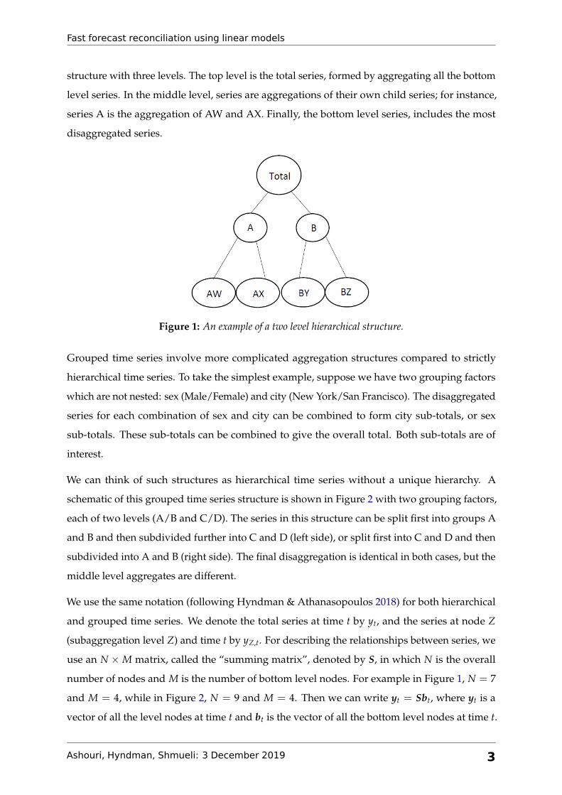
different types of food or drinks. Figure 1 shows a schematic of such a hierarchical time series

2

Fast forecast reconciliation using linear models

structure with three levels. The top level is the total series, formed by aggregating all the bottom

level series. In the middle level, series are aggregations of their own child series; for instance,

series A is the aggregation of AW and AX. Finally, the bottom level series, includes the most

disaggregated series.

Figure 1: An example of a two level hierarchical structure.

Grouped time series involve more complicated aggregation structures compared to strictly

hierarchical time series. To take the simplest example, suppose we have two grouping factors

which are not nested: sex (Male/Female) and city (New York/San Francisco). The disaggregated

series for each combination of sex and city can be combined to form city sub-totals, or sex

sub-totals. These sub-totals can be combined to give the overall total. Both sub-totals are of

interest.

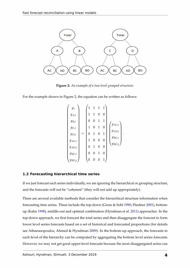
We can think of such structures as hierarchical time series without a unique hierarchy. A

schematic of this grouped time series structure is shown in Figure 2 with two grouping factors,

each of two levels (A/B and C/D). The series in this structure can be split first into groups A

and B and then subdivided further into C and D (left side), or split first into C and D and then

subdivided into A and B (right side). The final disaggregation is identical in both cases, but the

middle level aggregates are different.

We use the same notation (following Hyndman & Athanasopoulos 2018) for both hierarchical

and grouped time series. We denote the total series at time t by yt, and the series at node Z

(subaggregation level Z) and time t by yZ,t. For describing the relationships between series, we

use an N ×M matrix, called the “summing matrix”, denoted by S, in which N is the overall

number of nodes and M is the number of bottom level nodes. For example in Figure 1, N = 7

and M = 4, while in Figure 2, N = 9 and M = 4. Then we can write yt = Sbt, where yt is a

vector of all the level nodes at time t and bt is the vector of all the bottom level nodes at time t.

Ashouri, Hyndman, Shmueli: 3 December 2019 3


Figure 2: An example of a two level grouped structure.

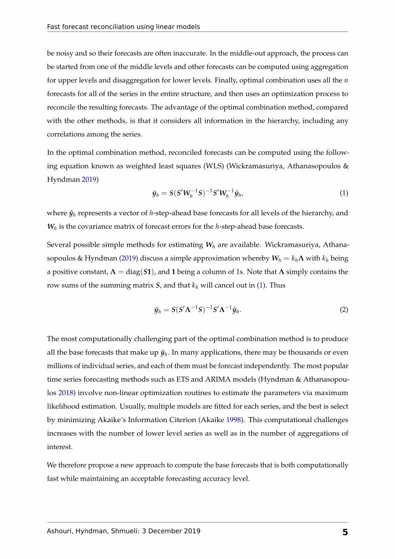
For the example shown in Figure 2, the equation can be written as follows:

yt

yA,t

yB,t

yC,t

yD,t

yAC,t

yAD,t

yBC,t

yBD,t

=

1 1 1 1

1 1 0 0

0 0 1 1

1 0 1 0

0 1 0 1

1 0 0 0

0 1 0 0

0 0 1 0

0 0 0 1

yAC,t

yAD,t

yBC,t

yBD,t

.

1.2 Forecasting hierarchical time series

If we just forecast each series individually, we are ignoring the hierarchical or grouping structure,

and the forecasts will not be “coherent” (they will not add up appropriately).

There are several available methods that consider the hierarchical structure information when

forecasting time series. These include the top-down (Gross & Sohl 1990; Fliedner 2001), bottom-

up (Kahn 1998), middle-out and optimal combination (Hyndman et al. 2011) approaches. In the

top-down approach, we first forecast the total series and then disaggregate the forecast to form

lower level series forecasts based on a set of historical and forecasted proportions (for details

see Athanasopoulos, Ahmed & Hyndman 2009). In the bottom-up approach, the forecasts in

each level of the hierarchy can be computed by aggregating the bottom level series forecasts.

However, we may not get good upper-level forecasts because the most disaggregated series can



be noisy and so their forecasts are often inaccurate. In the middle-out approach, the process can

be started from one of the middle levels and other forecasts can be computed using aggregation

for upper levels and disaggregation for lower levels. Finally, optimal combination uses all the n

forecasts for all of the series in the entire structure, and then uses an optimization process to

reconcile the resulting forecasts. The advantage of the optimal combination method, compared

with the other methods, is that it considers all information in the hierarchy, including any

correlations among the series.

In the optimal combination method, reconciled forecasts can be computed using the follow-

ing equation known as weighted least squares (WLS) (Wickramasuriya, Athanasopoulos &

Hyndman 2019)

yh = S(S′W−1h S)−1S′W−1

h yh, (1)

where yh represents a vector of h-step-ahead base forecasts for all levels of the hierarchy, and

Wh is the covariance matrix of forecast errors for the h-step-ahead base forecasts.

Several possible simple methods for estimating Wh are available. Wickramasuriya, Athana-

sopoulos & Hyndman (2019) discuss a simple approximation whereby Wh = khΛ with kh being

a positive constant, Λ = diag(S1), and 1 being a column of 1s. Note that Λ simply contains the

row sums of the summing matrix S, and that kh will cancel out in (1). Thus

yh = S(S′Λ−1S)−1S′Λ−1yh. (2)

The most computationally challenging part of the optimal combination method is to produce

all the base forecasts that make up yh. In many applications, there may be thousands or even

millions of individual series, and each of them must be forecast independently. The most popular

time series forecasting methods such as ETS and ARIMA models (Hyndman & Athanasopou-

los 2018) involve non-linear optimization routines to estimate the parameters via maximum

likelihood estimation. Usually, multiple models are fitted for each series, and the best is select

by minimizing Akaike’s Information Citerion (Akaike 1998). This computational challenges

increases with the number of lower level series as well as in the number of aggregations of

interest.

We therefore propose a new approach to compute the base forecasts that is both computationally

fast while maintaining an acceptable forecasting accuracy level.



2 Proposed approach: Linear model

Our proposed approach is based on using linear regression models for computing base forecasts.

Suppose we have a linear model that we use for forecasting, and we wish to apply it to N

different series which have some aggregation constraints. We have observations yt,i from times

t = 1, . . . , T and series i = 1, . . . , N. Then

yt,i = β′ixt,i + εt,i

where xt,i = {1, xt,i,1, . . . , xt,i,p} is a (p + 1)-vector of regression variables. This equation for all

the observations in matrix form can be written as follows:

y1

y2

y3...

yN

=

X1 0 0 . . . 0

0 X2 0 . . . 0

0 0 X3. . .

......

.... . . . . . 0

0 0 . . . 0 XN

β1

β2

β3...

βN

+

ε1

ε2

ε3...

εN

, (3)

where yi = {y1,i, y2,i, . . . , yT,i} is a T-vector, βi = {β0,i, β1,i, β2,i, . . . , βp,i} is a (p + 1)-vector,

εi = {ε1,i, ε2,i, . . . , εT,i} is a T-vector and Xi is the T × (p + 1)-matrix

Xi =

1 x1,i,1 x1,i,2 . . . x1,i,p

1 x2,i,1 x2,i,2 . . . x2,i,p...

......

...

1 xT,i,1 xT,i,2 . . . xT,i,p

.

Equation (3) can be written as Y = XB+ E, with parameter estimates given by B = (X ′X)−1X ′Y .

Then the base forecasts are obtained using

yt+h = X∗t+hB, (4)

where yt+h is an N-vector of forecasts, B comprises N stacked (p + 1)-vectors of estimated

coefficients, and X∗t+h is the N × N(p + 1) matrix



X∗t+h =

x′t+h,1 0 0 . . . 0

0 x′t+h,2 0 . . . 0

0 0 x′t+h,3. . .

......

.... . . . . . 0

0 0 . . . 0 x′t+h,N

.

Note that we use X∗t to distinguish this matrix, which combines xt,i across all series for one time

from Xi which combines xt,i across all time for one series.

Finally, we can combine the two linear equations for computing base forecasts and reconciled

forecasts (Equations (2) and (4)) to obtain the reconciled forecasts with a single equation:

yt+h = S(S′ΛS)−1S′Λ(X∗t+hB) = S(S′ΛS)−1S′ΛX∗t+h(X ′X)−1X ′Y . (5)

2.1 Simplified formulation for a fixed set of predictors (X)

If we have the same set of predictor variables, X, for all the series, we can write Equations (3) to

(5) more easily using multivariate regression equations, and we can obtain all the reconciled

forecasts for all the series in one equation. In that case, Equation (3) can be rearranged as follows:

y11 . . . y1N

y21 . . . y2N...

...

yT1 . . . yTN

=

1 X11 . . . X1p

1 X21 . . . X2p...

......

1 XT1 . . . XTp

β01 . . . β0N

β11 . . . β1N...

...

βp1 . . . βpN

+

ε11 . . . ε1N

ε21 . . . ε2N...

...

εT1 . . . εTN

, (6)

where Y , X, B and E are now matrices of size T × N, T × (p + 1), (p + 1) × N and T × N,

respectively. Equations (4) to (5) can be written accordingly using Equation (6) and here X∗t+h,i =

X∗t+h, where X∗t+h is an h× (p + 1) matrix.

2.2 OLS predictors

As an example of the Xt matrix in Equation (3), we can refer to the set of predictors proposed

in Ashouri, Shmueli & Sin (2018) for modeling trend, seasonality and autocorrelation by using

lagged values (yt−1, yt−2, . . . ), trend variables and seasonal dummy variables:

yt = α0 + α1t + β1s1,t + · · ·+ βm−1sm−1,t + γ1yt−1 + · · ·+ γpyt−p + δzt + εt. (7)



Here, sj,t is a dummy variable taking value 1 if time t is in season j (j = 1, 2, . . . , m), yt−k is the

kth lagged value for yt and zt is some external information at time t. The seasonal period m

depends on the problem; for instance, if we have daily data with day-of-week seasonality, then

m = 7.

Because of using lags and external series as predictors in Equation (7), we do not have same set

of predictors for all the series, yt. However, if we just use trend and seasonality dummies as

the predictors, then the simpler equations given in Section 2 can be written using multivariate

regression models.

While OLS is popular in practice for forecasting time series, it is often frowned upon due to

its independence assumption. This can cause issues for parametric inference but is less of a

problem for forecasting. In fact it often performs sufficiently well for forecasting as can be seen

by its popular use in practice. Further, the use of autoregressive terms in the above model

should model most of the autocorrelation in the data.

2.3 Computational considerations

There are two ways for computing the above forecasts. First, we could create the matrices Y , X

and E, and then directly use the above equations (taking advantage of sparse matrix routines)

to obtain the forecasts. Alternatively, we could use separate regression models to compute the

coefficients for each linear model individually. Although the matrix, X ′X, which we need to

invert is sparse and block diagonal, it is still faster to use the second approach involving separate

regression models.

2.4 Prediction intervals

For obtaining prediction intervals, we need to compute the variance of reconciled forecasts as

follows (Wickramasuriya, Athanasopoulos & Hyndman 2019):

Var(yt+h) = SPΣt+hP′S′, (8)

where P = (S′ΛS)−1S′Λ and Σt+h denotes the variance of the base forecasts given by the usual

linear model formula (Hyndman & Athanasopoulos 2018)

Σt+h = σ2[1 + X∗t+h(X ′X)−1(X∗t+h)

′]

.



Assuming normally distributed errors, we can easily obtain any required prediction intervals

corresponding to elements of yt+h using the diagonals of (8).

3 Applications

In this section we illustrate our approach using two examples: forecasting monthly Australian

domestic tourism and forecasting daily Wikipedia pageviews. We compare the forecasting

accuracy of ETS, ARIMA and the proposed linear OLS forecasting model, with and without

the reconciliation step. In these applications, we used the weighted reconciliation approach

from Equation (2). For comparing these methods, we use the average of Root Mean Square

Errors (RMSEs) across all series and also display box plots for forecast errors along with the raw

forecast errors.

The two datasets differ in terms of structure, size and behavior. The tourism data contains 304

series with both hierarchical and grouped structure, while the Wikipedia pageviews dataset

contains 913 series with grouped structure. The tourism dataset has strong seasonality while the

Wikipedia data are noiser.

We apply two methods for generating forecasts, which differ in how they handle unobserved

lagged values as inputs. The first approach is ex post in that it uses actual values, even when

they are future to the forecast origin. These values are known to us because they are in the test

set. We call these rolling origin forecasts. In the second ex ante method, we replace lagged values

of y by their forecasts if they occur at periods after the forecast origin. We call these fixed origin

forecasts.

3.1 Australian domestic tourism

This dataset has 19 years of monthly visitor nights in Australia by Australian tourists, a measure

used as an indicator of tourism activity (Wickramasuriya, Athanasopoulos & Hyndman 2019).

The data were collected by computer-assisted telephone interviews with 120,000 Australians

aged 15 and over (Tourism Research Australia 2005). The dataset includes 304 time series each

of length 228 observations. The hierarchy and grouping structure for this dataset is made using

geographic and purpose of travel information.

Table 1: Australia geographic hierarchical structure.

Series Name Label Series Name Label



Total Region

1 Australia Total 55 Lakes BCA

State 56 Gippsland BCB

2 NSW A 57 Phillip Island BCC

3 VIC B 58 General Murray BDA

4 QLD C 59 Goulburn BDB

5 SA D 60 High Country BDC

6 WA E 61 Melbourne East BDD

7 TAS F 62 Upper Yarra BDE

8 NT G 63 Murray East BDF

Zone 64 Wimmera+Mallee BEA

9 Metro NSW AA 65 Western Grampians BEB

10 Nth Coast NSW AB 66 Bendigo Loddon BEC

11 Sth Coast NSW AC 67 Macedon BED

12 Sth NSW AD 68 Spa Country BEE

13 Nth NSW AE 69 Ballarat BEF

14 ACT AF 70 Central Highlands BEG

15 Metro VIC BA 71 Gold Coast CAA

16 West Coast VIC BB 72 Brisbane CAB

17 East Coast VIC BC 73 Sunshine Coast CAC

18 Nth East VIC BD 74 Central Queensland CBA

19 Nth West VIC BE 75 Bundaberg CBB

20 Metro QLD CA 76 Fraser Coast CBC

21 Central Coast QLD CB 77 Mackay CBD

22 Nth Coast QLD CC 78 Whitsundays CCA

23 Inland QLD CD 79 Northern CCB

24 Metro SA DA 80 Tropical North Queensland CCC

25 Sth Coast SA DB 81 Darling Downs CDA

26 Inland SA DC 82 Outback CDB

27 West Coast SA DD 83 Adelaide DAA

28 West Coast WA EA 84 Barossa DAB

29 Nth WA EB 85 Adelaide Hills DAC

30 Sth WA EC 86 Limestone Coast DBA

31 Sth TAS FA 87 Fleurieu Peninsula DBB

32 Nth East TAS FB 88 Kangaroo Island DBC

33 Nth West TAS FC 89 Murraylands DCA

34 Nth Coast NT GA 90 Riverland DCB

35 Central NT GB 91 Clare Valley DCC

Region 92 Flinders Range and Outback DCD

36 Sydney AAA 93 Eyre Peninsula DDA

37 Central Coast AAB 94 Yorke Peninsula DDB

38 Hunter ABA 95 Australia’s Coral Coast EAA



39 North Coast NSW ABB 96 Experience Perth EAB

40 Northern Rivers Tropical NSW ABC 97 Australia’s SouthWest EAC

41 South Coast ACA 98 Australia’s North West EBA

42 Snowy Mountains ADA 99 Australia’s Golden Outback ECA

43 Capital Country ADB 100 Hobart and the South FAA

44 The Murray ADC 101 East Coast FBA

45 Riverina ADD 102 Launceston, Tamar and the North FBB

46 Central NSW AEA 103 North West FCA

47 New England North West AEB 104 Wilderness West FCB

48 Outback NSW AEC 105 Darwin GAA

49 Blue Mountains AED 106 Kakadu Arnhem GAB

50 Canberra AFA 107 Katherine Daly GAC

51 Melbourne BAA 108 Barkly GBA

52 Peninsula BAB 109 Lasseter GBB

53 Geelong BAC 110 Alice Springs GBC

54 Western BBA 111 MacDonnell GBD

Figure 3: Australian geographic hierarchical structure.

In this dataset we have three levels of geographic divisions in Australia. In the first level,

Australia is divided into seven “States” including New South Wales (NSW), Victoria (VIC),

Queensland (QLD), South Australia (SA), Western Australia (WA), Tasmania (TAS) and Northern

Territory (NT). In the second and third levels, it is divided into 27 “Zones” and 76 “Regions” (for

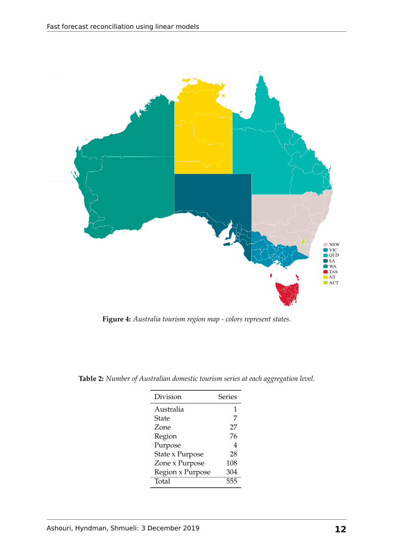
details about Australia geographic divisions see Figure 3 and Table 1 and also Figure 4 which

shows Australia map divided by tourism region and colored by states1).

We have four purposes of travel: Holiday (Hol), Visiting friends and relatives (Vis), Business

(Bus) and Other (Oth). So there are 76× 4 = 304 series at the most disaggregate level. Based on

the geographic hierarchy and purpose grouping, we end up with 8 aggregation levels with 555

series in total as shown in Table 2.1www.tra.gov.au/tra/2016/Tourism_Region_Profiles/Region_profiles/index.html


www.tra.gov.au/tra/2016/Tourism_Region_Profiles/Region_profiles/index.html


NSW

SA

VIC

NT

WA

QLD

TAS

ACT

Figure 4: Australia tourism region map - colors represent states.

Table 2: Number of Australian domestic tourism series at each aggregation level.

Division Series

Australia 1State 7Zone 27Region 76Purpose 4State x Purpose 28Zone x Purpose 108Region x Purpose 304Total 555



We report the forecast results for all these aggregation levels, as well as the average RMSE across

all the levels of the hierarchy. We used different predictors in the OLS predictor matrix for the

rolling and fixed origin approaches. For the rolling origin model, we included a linear trend, 11

dummy variables, and 12 lags. For the fixed origin model, we included a quadratic trend, 11

dummy variables, and lags 1 and 12. This is intended to capture the monthly seasonality. In

addition, before running the model, we partition the data into training and test sets, with the

last 24 months (2 years) as our test set, and the rest as our training set.

Table 3: Mean(RMSE) on 2 year test set for ETS, ARIMA and OLS with and without reconciliation -Rolling origin - Tourism dataset

Unreconciled Reconciled

Level ETS ARIMA OLS ETS ARIMA OLS

Total 1516.4 1445.5 1415.1 1517.2 1517.2 1414.7State 511.4 493.1 510.8 499.9 499.9 491.6Zone 214.8 219.0 224.5 209.6 209.6 213.6Region 122.9 125.1 124.0 119.4 119.4 120.4Purpose 676.0 709.2 694.5 674.2 674.2 681.9State x Purpose 213.1 220.1 216.1 212.7 212.7 213.3Zone x Purpose 97.5 102.4 101.0 96.8 96.8 99.0Region x Purpose 56.2 58.2 58.2 56.2 56.2 57.4

Table 4: Mean(RMSE) on 2 year test set for ETS, ARIMA and OLS with and without reconciliation -Fixed origin - Tourism dataset



Total 2238.6 3554.0 2528.9 2232.8 3460.3 2540.1State 593.6 570.1 596.5 555.7 658.5 579.0Zone 239.5 229.6 243.3 235.3 249.8 235.4Region 132.6 129.4 127.1 127.6 132.4 123.8Purpose 766.8 824.0 875.5 801.7 1019.3 857.2State x Purpose 226.7 241.2 236.7 224.5 245.6 229.1Zone x Purpose 103.0 105.4 104.9 102.4 105.8 102.9Region x Purpose 59.1 58.8 58.6 58.8 59.3 57.9

In Figures 5 and 6 we display the error box plots for both reconciled and unreconciled forecasts

using all three methods, for the rolling origin and fixed origin forecasts. In these figures we see

the error distributions across all the models.

Together with Tables 3 and 4, results show that our proposed OLS forecasting model produces

forecast accuracy similar to ETS and ARIMA, which are computationally heavy for many time

series. We also see the usefulness of the reconciliation in decreasing the average RMSE in all three

methods. Except for the total series, reconciliation improves forecasts in all the hierarchy levels.



Purpose State x Purpose Zone x Purpose Region x Purpose

Total State Zone Region

ETS.rec

ETS.unr

ec

ARIMA.re

c

ARIMA.u

nrec

OLS.re

c

OLS.u

nrec

ETS.rec

ETS.unr

ec

ARIMA.re

c

ARIMA.u

nrec

OLS.re

c

OLS.u

nrec

ETS.rec

ETS.unr

ec

ARIMA.re

c

ARIMA.u

nrec

OLS.re

c

OLS.u

nrec

ETS.rec

ETS.unr

ec

ARIMA.re

c

ARIMA.u

nrec

OLS.re

c

OLS.u

nrec

−500

0

500

1000

−400

0

400

800

−1000

−500

0

500

1000

1500

−500

0

500

−1000

0

1000

2000

−1000

−500

0

500

1000

−2000

−1000

0

1000

2000

3000

−1000

0

1000

2000

Method

Err

or

Figure 5: Box plots of rolling origin forecast errors from reconciled and unreconciled ETS, ARIMA andOLS methods at each hierarchical level for tourism demand.



ETS.rec

ETS.unr

ec

ARIMA.re

c

ARIMA.u

nrec

OLS.re

c

OLS.u

nrec

ETS.rec

ETS.unr

ec

ARIMA.re

c

ARIMA.u

nrec

OLS.re

c

OLS.u

nrec

ETS.rec

ETS.unr

ec

ARIMA.re

c

ARIMA.u

nrec

OLS.re

c

OLS.u

nrec

ETS.rec

ETS.unr

ec

ARIMA.re

c

ARIMA.u

nrec

OLS.re

c

OLS.u

nrec

−1000

−500

0

500

1000

−400

0

400

800

−1000

0

1000

−500

0

500

−1000

0

1000

2000

−1000

−500

0

500

1000

0

2000

4000

6000

−1000

0

1000

2000

3000

Method

Err

or

Figure 6: Box plots of fixed origin forecast errors for reconciled and unreconciled ETS, ARIMA and OLSmethods at each hierarchical level for tourism demand.



Also, because the higher level series have higher counts, the errors are larger in magnitude

(Appendix A shows the box plots with scaled errors, to better compare errors across all the

hierarchy levels). In addition, we see that (as expected) by applying rolling origin 1-step-ahead

forecasts, the error densities are closer and more tightly distributed around zero than the fixed

origin multi-step-ahead forecasts.

Figures 7 and 8 show the rolling and fixed origin forecast results for the total series and one of

the bottom level series, BACBus (Geelong - Business). In these plots we have both reconciled

(solid lines) and unreconciled (dashed lines) forecasts and we see that the reconciliation step

improves the forecasts in this series. We also see that the OLS model forecast accuracy is similar

to the other two methods.

20000

30000

40000

0 5 10 15 20 25Horizon

Cou

nt

Series

Actual

ARIMA

ETS

OLS

Rolling origin 1−step forecasts

20000

30000

40000

0 5 10 15 20 25Horizon

Cou

nt

Reconciled

Actual

rec

unrec

Fixed origin multi−step forecasts

Figure 7: The actual test set for the ’Total series’ compared to the forecasts from reconciled and unrecon-ciled ETS, ARIMA and OLS methods for rolling and fixed origin tourism demand.

Table 5 compares the computation time of the three methods for rolling and fixed origin fore-

casting. We see that the OLS forecasting model is much faster compared to the other methods.

Also, since reconciliation is a linear process, in all methods it is very fast and does not affect

computation time significantly.

Since we are using a linear model, we can easily include exogenous variables which can often

be helpful in improving forecast accuracy. In this application, we tried including an “Easter”



0

20

40

60

0 5 10 15 20 25Horizon

Cou

nt

Series

Actual

ARIMA

ETS

OLS


0

20

40

60

0 5 10 15 20 25Horizon

Cou

nt

Reconciled

Actual

rec

unrec


Figure 8: The actual test set for the ’BACBus’ bottom level series compared to the forecasts from reconciledand unreconciled ETS, ARIMA and OLS methods for rolling and fixed origin tourism demand.

Table 5: Computation time (seconds) for ETS, ARIMA and OLS with and without reconciliation -Rolling and fixed origin forecasts on a 24 month test set - Tourism dataset

Rolling origin Fixed origin

Unreconciled Reconciled Unreconciled Reconciled

ETS 10924.57 10924.60 407.10 407.15ARIMA 31146.38 31146.52 1116.15 1116.19OLS 48.40 48.31 17.42 17.80

dummy variable indicating the timing of Easter, but its affect on forecast accuracy was minimal,

so it was omitted in the model reported here.

Finally, Table 6 shows that, as mentioned in Section 2.3, computation is faster using separate

regression models compared to the matrix approach (even using sparse matrix algebra).

Table 6: Computation time (seconds) for OLS using the matrix approach and separate regression models,with and without reconciliation, on a rolling and fixed origin for 24 steps ahead.



Matrix approach 202.06 209.84 87.73 105.69Separate models 48.40 48.31 16.66 16.85



3.2 Wikipedia pageviews: Grouped structure

The second dataset comprises one year of daily data (2016-06-01 to 2017-06-29) on Wikipedia

pageviews for the most popular social networks articles (Ashouri, Shmueli & Sin 2018). This

dataset is noisier than the Australian monthly tourism data, making forecasting more chal-

lenging. The data has a grouped structure with the following attributes: “Agent”: Spider,

User, “Access”: Desktop, Mobile app, Mobile web, “Language”: en (English), de (German), es

(Spanish), zh (Chinese) and “Purpose”: Blogging related, Business, Gaming, General purpose,

Life style, Photo sharing, Reunion, Travel, Video (see Table 7).

Table 7: Social networking Wikipedia article grouping structure

Grouping Series Grouping Series

Total Language1. Social Network 10. zh (Chinese)

Access Purpose2. Desktop 11. Blogging related3. Mobile app 12. Business

Agent 13. Gaming4. Mobile web 14. General purpose5. Spider 15. Life style6. User 16. Photo sharing

Language 17. Reunion7. en (English) 18. Travel8. de (German) 19. Video9. es (Spanish)

We consider the main aggregation factors and two-way combinations of them. The final dataset

includes 913 time series, each with length 394. The applied group structure and different levels

include the following aggregations:2

• Total

• Access

• Agent

• Language

• Purpose

• Access × Agent

• Access × Language

• Access × Purpose

2There are four more 3-way aggregation combinations that we do not include: Agent × Access × Language,Agent × Access × Purpose, Agent × Language × Purpose, and Access × Language × Purpose. Including these fouradditional aggregations might slightly improve the results but for simplicity, we excluded them.



• Agent × Language

• Agent × Purpose

• Language × Purpose

• Bottom level: Access × Agent × Language × Purpose

For this daily dataset, in the OLS forecasting model we include in the predictor matrix a

quadratic trend, 6 seasonal dummies and all 7 lags for rolling, and for fixed origin model we use

a quadratic trend, 6 seasonal dummies and lags 1 and 7. We partitioned the data into two parts

training and test sets. We used the last 28 days for our test set and the rest for the training set. In

this example, the results in tables and figures are represented for single groups although we

applied all the above levels in the group structure for reconciliation.

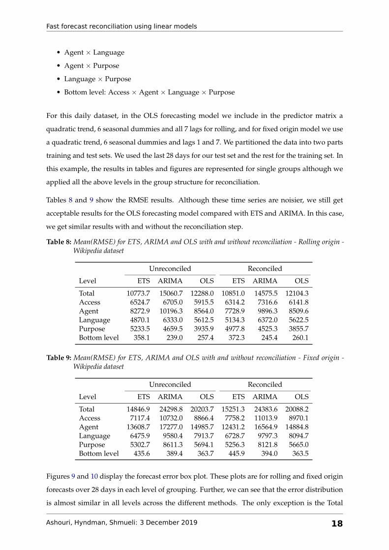
Tables 8 and 9 show the RMSE results. Although these time series are noisier, we still get

acceptable results for the OLS forecasting model compared with ETS and ARIMA. In this case,

we get similar results with and without the reconciliation step.

Table 8: Mean(RMSE) for ETS, ARIMA and OLS with and without reconciliation - Rolling origin -Wikipedia dataset



Total 10773.7 15060.7 12288.0 10851.0 14575.5 12104.3Access 6524.7 6705.0 5915.5 6314.2 7316.6 6141.8Agent 8272.9 10196.3 8564.0 7728.9 9896.3 8509.6Language 4870.1 6333.0 5612.5 5134.3 6372.0 5622.5Purpose 5233.5 4659.5 3935.9 4977.8 4525.3 3855.7Bottom level 358.1 239.0 257.4 372.3 245.4 260.1

Table 9: Mean(RMSE) for ETS, ARIMA and OLS with and without reconciliation - Fixed origin -Wikipedia dataset



Total 14846.9 24298.8 20203.7 15251.3 24383.6 20088.2Access 7117.4 10732.0 8866.4 7758.2 11013.9 8970.1Agent 13608.7 17277.0 14985.7 12431.2 16564.9 14884.8Language 6475.9 9580.4 7913.7 6728.7 9797.3 8094.7Purpose 5302.7 8611.3 5694.1 5256.3 8121.8 5665.0Bottom level 435.6 389.4 363.7 445.9 394.0 363.5

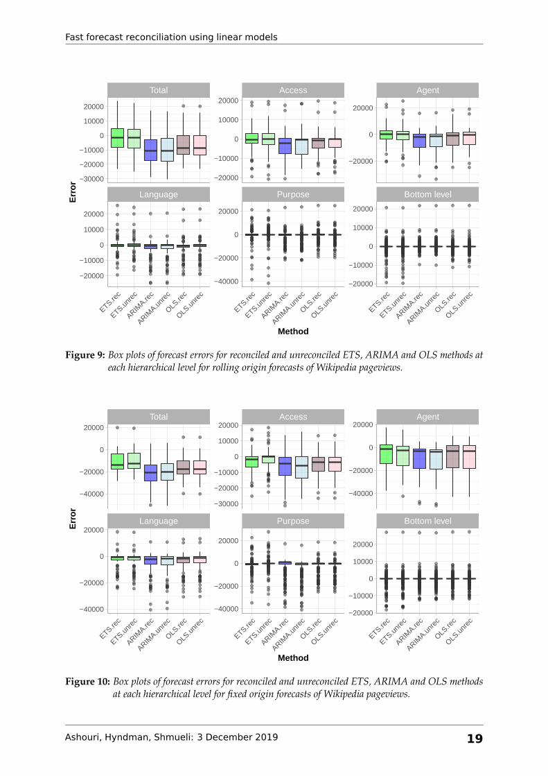
Figures 9 and 10 display the forecast error box plot. These plots are for rolling and fixed origin

forecasts over 28 days in each level of grouping. Further, we can see that the error distribution

is almost similar in all levels across the different methods. The only exception is the Total



Language Purpose Bottom level

Total Access Agent

ETS.rec

ETS.unr

ec

ARIMA.re

c

ARIMA.u

nrec

OLS.re

c

OLS.u

nrec

ETS.rec

ETS.unr

ec

ARIMA.re

c

ARIMA.u

nrec

OLS.re

c

OLS.u

nrec

ETS.rec

ETS.unr

ec

ARIMA.re

c

ARIMA.u

nrec

OLS.re

c

OLS.u

nrec

−20000

0

20000

−20000

−10000

0

10000

20000

−20000

−10000

0

10000

20000

−40000

−20000

0

20000

−30000

−20000

−10000

0

10000

20000

−20000

−10000

0

10000

20000

Method

Err

or

Figure 9: Box plots of forecast errors for reconciled and unreconciled ETS, ARIMA and OLS methods ateach hierarchical level for rolling origin forecasts of Wikipedia pageviews.

Language Purpose Bottom level

Total Access Agent

ETS.rec

ETS.unr

ec

ARIMA.re

c

ARIMA.u

nrec

OLS.re

c

OLS.u

nrec

ETS.rec

ETS.unr

ec

ARIMA.re

c

ARIMA.u

nrec

OLS.re

c

OLS.u

nrec

ETS.rec

ETS.unr

ec

ARIMA.re

c

ARIMA.u

nrec

OLS.re

c

OLS.u

nrec

−40000

−20000

0

20000

−20000

−10000

0

10000

20000

−30000

−20000

−10000

0

10000

20000

−40000

−20000

0

20000

−40000

−20000

0

20000

−40000

−20000

0

20000

Method

Err

or

Figure 10: Box plots of forecast errors for reconciled and unreconciled ETS, ARIMA and OLS methodsat each hierarchical level for fixed origin forecasts of Wikipedia pageviews.



190000

210000

230000

0 10 20Horizon

Cou

nt

Series

Actual

ARIMA

ETS

OLS


190000

210000

230000

0 10 20Horizon

Cou

nt

Reconciled

Actual

rec

unrec


Figure 11: The actual test set for the ’Total’ series compared to the forecasts from reconciled and unrec-onciled ETS, ARIMA and OLS methods for rolling and fixed origin forecasts of Wikipediapageviews.

400

600

800

1000

1200

0 10 20Horizon

Cou

nt

Series

Actual

ARIMA

ETS

OLS


400

600

800

1000

1200

0 10 20Horizon

Cou

nt

Reconciled

Actual

rec

unrec


Figure 12: The actual test set for the ’desktopusenPho04’ bottom level series compared to the forecastsfrom reconciled and unreconciled ETS, ARIMA and OLS methods for rolling and fixed originforecasts of Wikipedia pageviews.



series, where ETS performs significantly better than ARIMA and OLS. We also note that the

reconciliation is less effective. As in the tourism example, in higher levels, series have higher

counts and therefore their error magnitudes are larger.

In Figures 11 and 12, we display results for the total and one of the bottom level series, “desk-

topusenPho04” (desktop-user-english-photo sharing). The plot shows rolling and fixed origin

forecast results over the 28 day test set for ETS, ARIMA and OLS, with (solid lines) and without

(dashed lines) applying reconciliation. We see that the OLS forecasting model performs close to

the other two methods, and reconciliation improves the forecasts.

Table 10 presents the computation times for all three methods. ETS and ARIMA are clearly

much more computationally heavy compared with OLS. As in the Australian tourism dataset,

running reconciliation does not have much effect on computation time.

Table 10: Computation time (seconds) for ETS, ARIMA and OLS with and without reconciliation -Rolling and fixed origin forecasts - Wikipedia dataset

Computation time (secs)



ETS 27613.08 27613.14 971.55 971.58ARIMA 49419.36 49419.39 1769.52 1769.56

OLS 116.27 116.31 61.33 61.38

4 Conclusion

We have proposed a linear model approach to fast forecasting of hierarchical or grouped time

series, with accuracy that nearly matches that of forecast methods such as ETS and ARIMA. This

is especially useful in large collections of time series, as is typical in hierarchical and grouped

structures. Although ETS and ARIMA are advantageous in terms of forecasting power and

accuracy, they can be computationally heavy when facing large collections of time series in the

hierarchy. An important feature of our model is its ability to easily include external information

such as holiday dummies or other external series. We also note that OLS has the additional

practical advantage of handling missing data while ETS requires imputation.

Another advantage of our approach is that it can be computed in a single matrix equation (5).

This makes it extremely fast and easy to implement, and enables standard results to be derived

with minimal effort (e.g., prediction intervals).



Pennings & Dalen (2017) proposed another approach for forecasting hierarchical time series

using state space models. Although their approach is flexible in handling outliers, missing data

and external features, it is less flexible to different kinds of datasets and it is computationally

much more complex.

Acknowledgements

The first and third authors of this research were partially funded by Ministry of Science and

Technology (MOST), Taiwan [Grant 106-2420-H-007-019].



Appendix A

We provide boxplots of the scaled forecasted errors for the tourism example. These plots are

displayed for both rolling forward and multiple-step-ahead forecasts.



ETS.rec

ETS.unr

ec

ARIMA.re

c

ARIMA.u

nrec

OLS.re

c

OLS.u

nrec

ETS.rec

ETS.unr

ec

ARIMA.re

c

ARIMA.u

nrec

OLS.re

c

OLS.u

nrec

ETS.rec

ETS.unr

ec

ARIMA.re

c

ARIMA.u

nrec

OLS.re

c

OLS.u

nrec

ETS.rec

ETS.unr

ec

ARIMA.re

c

ARIMA.u

nrec

OLS.re

c

OLS.u

nrec

−2.5

0.0

2.5

5.0

−2.5

0.0

2.5

5.0

Method

Err

or

Figure 13: Box plots of scaled forecast errors from reconciled and unreconciled ETS, ARIMA and OLSmethods at each hierarchical level for rolling origin 1-step-ahead tourism demand.



ETS.rec

ETS.unr

ec

ARIMA.re

c

ARIMA.u

nrec

OLS.re

c

OLS.u

nrec

ETS.rec

ETS.unr

ec

ARIMA.re

c

ARIMA.u

nrec

OLS.re

c

OLS.u

nrec

ETS.rec

ETS.unr

ec

ARIMA.re

c

ARIMA.u

nrec

OLS.re

c

OLS.u

nrec

ETS.rec

ETS.unr

ec

ARIMA.re

c

ARIMA.u

nrec

OLS.re

c

OLS.u

nrec

−2.5

0.0

2.5

5.0

−2.5

0.0

2.5

5.0

Method

Err

or

Figure 14: Box plots of scaled forecast errors from reconciled and unreconciled ETS, ARIMA and OLSmethods at each hierarchical level for fixed origin multi-step-ahead tourism demand.



References

Akaike, H (1998). “Information theory and an extension of the maximum likelihood principle”.

In: Selected Papers of Hirotugu Akaike. Springer Series in Statistics (Perspectives in Statistics).

Springer, pp.199–213.

Ashouri, M, G Shmueli & CY Sin (2018). Clustering time series by domain-relevant features

using model-based trees. Proceedings of the 2018 Data Science, Statistics & Visualization (DSSV).

Athanasopoulos, G, RA Ahmed & RJ Hyndman (2009). Hierarchical forecasts for Australian

domestic tourism. International Journal of Forecasting 25(1), 146–166.

Fliedner, G (2001). Hierarchical forecasting: issues and use guidelines. Industrial Management &

Data Systems 101(1), 5–12.

Gross, CW & JE Sohl (1990). Disaggregation methods to expedite product line forecasting. Journal

of Forecasting 9(3), 233–254.

Hyndman, RJ, RA Ahmed, G Athanasopoulos & HL Shang (2011). Optimal combination forecasts

for hierarchical time series. Computational Statistics & Data Analysis 55(9), 2579–2589.

Hyndman, RJ & G Athanasopoulos (2018). Forecasting: principles and practice. Melbourne, Aus-

tralia: OTexts. https://OTexts.org/fpp2.

Kahn, KB (1998). Revisiting top-down versus bottom-up forecasting. The Journal of Business

Forecasting 17(2), 14.

Pennings, CL & J van Dalen (2017). Integrated hierarchical forecasting. European Journal of

Operational Research 263(2), 412–418.

Tourism Research Australia (2005). Travel by Australians, September Quarter 2005. Tourism

Australia.

Wickramasuriya, SL, G Athanasopoulos & RJ Hyndman (2019). Optimal forecast reconciliation

for hierarchical and grouped time series through trace minimization. Journal of the American

Statistical Association 14(526), 804–819.


https://OTexts.org/fpp2

Fast forecast reconciliation using linear models

Documents

Transcript of Fast forecast reconciliation using linear models