© 2019 Institute of Physics and Engineering in Medicine

1. Introduction

Brain imaging using high resolution magnetic resonance imaging (MRI) has expanded the role of neuroimaging in clinical and research setting, particularly when used in junction with advanced data extraction and visualization tools. The accurate interpretation of information pertaining to investigate the aging brain or disease induced brain alterations, as well as functional studies of brain tissues relies on accurate and reproducible brain tissue classification, which is the preliminary step prior to segmentation (Pham et al 2000, Sonka and Fitzpatrick 2000). Manual tissues classification may be reliable, but is difficult to perform in clinical routine and is time consuming (Hatt et al 2017). Furthermore, it suffers from large intra- and inter-observer variability that decreases the credibility of segmentation-based image analysis (Kasiri et al 2010). As such, there is a large demand to develop alternative methods for robust and accurate automated classification of brain MR images as a prerequisite for

C Fatnassi and H Zaidi

Printed in the UK

145005

PHMBA7

© 2019 Institute of Physics and Engineering in Medicine

64

Phys. Med. Biol.

PMB

1361-6560

10.1088/1361-6560/ab239e

14

1

16

Physics in Medicine & Biology

IOP

11

July

2019

Fast and accurate pseudo multispectral technique for whole-brain MRI tissue classification

Chemseddine Fatnassi1 and Habib Zaidi1,2,3,4,5

1 Division of Nuclear Medicine and Molecular Imaging, Geneva University Hospital, CH-1211 Geneva, Switzerland2 Geneva University Neurocenter, Geneva University, CH-1205 Geneva, Switzerland3 Department of Nuclear Medicine and Molecular Imaging, University of Groningen, University Medical Center Groningen, 9700RB

Groningen, The Netherlands4 Department of Nuclear Medicine, University of Southern Denmark, DK-500, Odense, Denmark5 Author to whom any correspondence should be addressed.

E-mail: habib.zaidi@hcuge.ch

Keywords: MRI, segmentation, brain tissue classification, color spaces, contrast enhancement

AbstractNumerous strategies have been proposed to classify brain tissues into gray matter (GM), white matter (WM) and cerebrospinal fluid (CSF). However, many of them fail when classifying specific regions with low contrast between tissues. In this work, we propose an alternative pseudo multispectral classification (PMC) technique using CIE LAB spaces instead of gray scale T1-weighted MPRAGE images, combined with a new preprocessing technique for contrast enhancement and an optimized iterative K-means clustering. To improve the accuracy of the classification process, gray scale images were converted to multispectral CIE LAB data by applying several transformation matrices. Thus, the amount of information associated with each image voxel was increased. The image contrast was then enhanced by applying a real time function that separates brain tissue distributions and improve image contrast in certain brain regions. The data were then classified using an optimized iterative and convergent K-means classifier. The performance of the proposed approach was assessed using simulation and in vivo human studies through comparison with three common software packages used for brain MR image segmentation, namely FSL, SPM8 and K-means clustering. In the presence of high SNR, the results showed that the four algorithms achieve a good classification. Conversely, in the presence of low SNR, PMC was shown to outperform the other methods by accurately recovering all tissue volumes. The quantitative assessment of brain tissue classification for simulated studies showed that the PMC algorithm resulted in a mean Jaccard index (JI) of 0.74 compared to 0.75 for FSL, 0.7 for SPM and 0.8 for K-means. The in vivo human studies showed that the PMC algorithm resulted in a mean JI of 0.92, which reflects a good spatial overlap between segmented and actual volumes, compared to 0.84 for FSL, 0.78 for SPM and 0.66 for K-means. The proposed algorithm presents a high potential for improving the accuracy of automatic brain tissues classification and was found to be accurate even in the presence of high noise level.

PAPER2019

RECEIVED 20 January 2019

REVISED

19 May 2019

ACCEPTED FOR PUBLICATION

22 May 2019

PUBLISHED 11 July 2019

https://doi.org/10.1088/1361-6560/ab239ePhys. Med. Biol. 64 (2019) 145005 (16pp)

2

C Fatnassi and H Zaidi

brain function analysis. Image segmentation involves partitioning an image into non-overlapped regions, which are homogeneous in regard to specific criterions, such as tissue texture or intensity level. If the image is indicated as ‘I’, the segmentation problem consists in estimating a set 𝑆𝑘 ∈ 𝐼 that can be used to build an image ‘I’ satisfying the condition:

I =N⋃

k=1

Sk.

Classification is a particular case of segmentation where the restriction for spatial connectivity for all points belonging to a given n 𝑆𝑘 is removed. The resulting sets in this case are called classes. The classification accuracy is highly influenced by the class number estimation, which may be very complicated. A reproducible classes labe-ling may also be a hard task without previous knowledge about the images.

Numerous algorithms with different degrees of success have been proposed to classify brain tissues into gray matter (GM), white matter (WM) and cerebrospinal fluid (CSF). This includes atlas-free techniques or methods relying on the use of an atlas. A couple of existing principal approaches are based on histogram threshold deter-mination (Suzuki and Toriwaki 1991), cluster analysis (Simmons et al 1994), a prior information about anatomy (Joliot and Mazoyer 1993), Bayesian classification (e.g. Markov Random field model) (Chang et al 1996) and deep learning-based approaches (Moeskops et al 2016, Dolz et al 2017, Chen et al 2018, Wachinger et al 2018). An overview of brain MRI classification algorithms can be found in recent reviews on the topic (Clarke et al 1995, Cabezas et al 2011, Selvaraj and Dhanasekaran 2013, Gonzalez-Villa et al 2016, Helms 2016). Some of these techniques produce good results but fail in some regions where the contrast is low, such as medial temporal lobe region and cerebellum where the arbor vitae (WM) and GM interfaces are difficult to classify.

Currently, different software packages are available to the neuroimaging community. These tools commonly contain a set of preprocessing steps, such as skull stripping, data denoising and bias field correction, in addition to performing automated brain tissues classification. Among them, the statistical parametric mapping (SPM) toolbox (Ashburner et al 1995) developed by the Wellcome Trust Centre for Neuroimaging, University College London (UK), FMRIB’s Software Library (FSL) software package (Smith et al 2004, Woolrich et al 2009, Jenkin-son et al 2012) developed by the Analysis Group at Oxford Centre for functional MRI of the brain (FMRIB) and the K-means clustering algorithm (Spath 1985, David and Vassilvitskii 2007, Seber 2008) are the most widely used. Most of the proposed methods usually take as input one channel gray scale data, which may limit features that we can use to classify image pixels and may be inadequate to maintain fine description compared to other color spaces.

In this work, we introduce a novel method combining pseudo-multispectral color transformation, a set of preprocessing techniques for contrast enhancement and an iterative and optimized K-means clustering to improve brain tissue classification even in the presence of low signal to noise ratio (SNR) and high partial vol-ume effect. The performance of the proposed algorithm using both simulated and in vivo human studies with frequently used evaluation metrics was assessed. A detailed comparison with SPM, FSL and K-means algorithms was also performed.

2. Theory

2.1. Multispectral color transformationColor models or color spaces indicate the colors in a benchmark way by using a coordinate system and a subspace in which each color is represented by a single voxel of the coordinate system. Gray and binary color spaces are commonly used by image processing methods (Gonzalez et al 2004, Cui et al 2005). The contrast between brain tissues in some regions is, however, very low, e.g. cerebellum (WM and GM interfaces). Consequently, well-known techniques almost fail and wrong classifications might occur. Furthermore, additional filtering may smooth the data and lead to spatial resolution loss. To address this issue, we considered appropriately enhancing the amount of information passed to the classifier. To this end, the first step consists in transforming the T1-weighted MPRAGE images to multispectral data containing three different images (channels), rather than classifying using single image information (e.g. gray scale image). In other words, each voxel in the initial image was represented in three different coordinate spaces. Firstly, the gray scale image was converted to an RGB color image, which employed the RGB color space consisting of three bands: red, green and blue. Consequently, each pixel will be represented by an n-valued vector instead of one, where n is the number of bands, for instance, a three-value vector [r,g,b] in case of color images. Secondly, the RGB images are converted to CIE XYZ space and then to CIE LAB space by applying a number of mathematical operations described in Rhyne (2016). These routines convert images back and forth from RGB to CIE LAB color spaces by rescaling the image color spaces. These numerical functions implemented in C (Insight Segmentation and Registration Toolkit ITK) or in Matlab code (MathWorks Inc., Natick, MA) are available as open source software. We should keep in mind that the transformation between the two spaces is not unique. The resulting CIE LAB may be scaled differently if a slightly different coefficients

Phys. Med. Biol. 64 (2019) 145005 (16pp)

3

C Fatnassi and H Zaidi

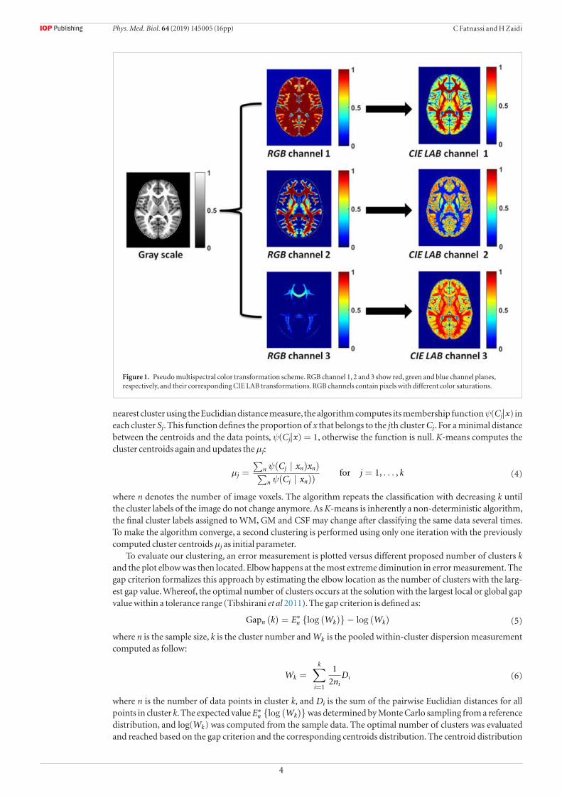
or transformation parameters are used during processing. Therefore, we strongly recommend the use of the implemented default conversion parameters. The International Commission on Illumination (CIE) color spaces were the first well defined mathematical quantitative connections between wavelength distributions in the electromagnetic visible spectrum, and physiologically perceived colors in the human color vision (Sève 1996). The CIE LAB color space (also known as CIE L * a * b* or sometimes abbreviated simply as ‘Lab’ color space) is a color-space introduced in 1976 by the CIE, considered as an enhanced version of CIE XYZ tristimuls color space. For more detailed description, we refer interested readers to (Lindsey and Wee 2007). It describes color in three numerical values, ‘L’ for brightness and ‘a*b*’ for green-red and blue-color components. The L*a*b term may also express the difference in color compared to that of a gray surface of the same clarity. Figure 1 illustrates the pseudo-multispectral color transformation scheme. In RGB images, each separated color plane contains some saturated pixels that represent the highest concentration of pure red, green or blue values. As the color becomes mixed with other colors, low intensity pixels appear. We should keep in mind that color space transformation only transforms image color spaces and no tissue classifications is yet performed.

2.2. Root and square function (RSF) approachPoor image quality may challenge the classification process. Therefore, image enhancement remains a necessary step prior to data classification and segmentation. These improvements include correcting the data for unwanted noise, skull stripping and contrast enhancement. This can be achieved using a number of denoising approaches, such as the use of conventional to more advanced filters, nonlinear filtering approaches (Cui et al 2005), anisotropic nonlinear diffusion filtering (Weickert et al 1998), wavelet denoising and Markov random field modeling (Xie et al 2002) and more recently hybrid spatial-frequency domain filtering (Arabi and Zaidi 2018). Denoising the images without a priori knowledge of the noise distribution may, however, compromise image quality by smoothing the edge interface between gray and WM regions, thereby leading to contrast losses between fine structures, which, in turn, can present major challenges for accurate classification and segmentation of these regions (Mohan et al 2014).

Contrast enhancement methods are divided into two main approaches: direct and indirect (Gonzalez and Woods 2002, Russ 2011). In direct approaches, the image contrast is displayed then enhanced by means of some transformation functions, such as the dynamic range of the display device (Gonzalez and Woods 2002). Con-versely, indirect methods involve performing contrast stretching using linear and nonlinear functions (Xu et al 2010, Jafar and Darabkh 2011), histogram equalization and specification (Iqbal et al 2007) and gray level group-ing (Chen et al 2006). Overall, contrast enhancement has advantages and drawbacks. It may improve global image quality, however, it usually fails to enhance local details or can lead to noise amplification (Mohan et al 2014).

To overcome these problems, we propose a new real time approach to enhance the image contrast especially in WM, GM and CSF interfaces entitled RSF. The RSF is based on the following principle:

‖xn − xn+1‖ <∥∥xαn − xαn+1

∥∥ (1)

where xn is the intensity of the nth voxel and α is a real positive number (α > 1). The principle tells us that the distance between two neighboring intensities is smaller than the distance between their intensities to the α power. Thus, the image contrast enhancement may be performed by applying RSF on the MR image as described below:

IMRSF =

® √xn, xn < 0.5

xβ+1/2n , xn � 0.5

(2)

where IMRSF is the enhanced image, xn is the intensity of the nth MR image voxel, β is a positive integer number. In this study, β is iteratively computed to achieve the best WM, GM and CSF distribution separation. The RSF was applied on CIE LAB channels, which enhances the interfaces sharpness between the three brain tissues, especially in regions with low SNR without noise amplification.

2.3. Data clusteringBefore clustering, the brain tissue was extracted out of the structural image using the brain extraction tool (BET) (Smith 2002). As first clustering, an iterative and non-deterministic K-means clustering was applied for image classification. Initially, the number of brain tissue classes was randomly chosen and set to be maximal (>5 classes). The K-means clustering algorithm clusters the enhanced three channel CIE LAB data around centroids computed as the mean value of clustered points so as to minimize the within-cluster sum of squares as follows:

arg min∑

N

k∑i=1

∑x∈Sj

∥∥xN,i,Sj − µi

∥∥2 (3)

where µi is the mean of data points x within Sj partitions, k is the number of clusters and N is the enhanced 3D channel images (N is one of the three channels in CIE LAB color space). After assigning each data point x to the

Phys. Med. Biol. 64 (2019) 145005 (16pp)

4

C Fatnassi and H Zaidi

nearest cluster using the Euclidian distance measure, the algorithm computes its membership function ψ(Cj |x) in each cluster Sj. This function defines the proportion of x that belongs to the j th cluster Cj . For a minimal distance between the centroids and the data points, ψ(Cj |x) = 1, otherwise the function is null. K-means computes the cluster centroids again and updates the µj:

µj =

∑n ψ(Cj | xn)xn)∑

n ψ(Cj | xn))for j = 1, . . . , k (4)

where n denotes the number of image voxels. The algorithm repeats the classification with decreasing k until the cluster labels of the image do not change anymore. As K-means is inherently a non-deterministic algorithm, the final cluster labels assigned to WM, GM and CSF may change after classifying the same data several times. To make the algorithm converge, a second clustering is performed using only one iteration with the previously computed cluster centroids µj as initial parameter.

To evaluate our clustering, an error measurement is plotted versus different proposed number of clusters k and the plot elbow was then located. Elbow happens at the most extreme diminution in error measurement. The gap criterion formalizes this approach by estimating the elbow location as the number of clusters with the larg-est gap value. Whereof, the optimal number of clusters occurs at the solution with the largest local or global gap value within a tolerance range (Tibshirani et al 2011). The gap criterion is defined as:

Gapn (k) = E∗n {log (Wk)} − log (Wk) (5)

where n is the sample size, k is the cluster number and Wk is the pooled within-cluster dispersion measurement computed as follow:

Wk =k∑

i=1

1

2niDi (6)

where n is the number of data points in cluster k, and Di is the sum of the pairwise Euclidian distances for all points in cluster k. The expected value E∗

n {log (Wk)} was determined by Monte Carlo sampling from a reference distribution, and log(Wk) was computed from the sample data. The optimal number of clusters was evaluated and reached based on the gap criterion and the corresponding centroids distribution. The centroid distribution

Figure 1. Pseudo multispectral color transformation scheme. RGB channel 1, 2 and 3 show red, green and blue channel planes, respectively, and their corresponding CIE LAB transformations. RGB channels contain pixels with different color saturations.

Phys. Med. Biol. 64 (2019) 145005 (16pp)

5

C Fatnassi and H Zaidi

was modeled beforehand using a set of 20 human brain data. Each brain tissue class (GM, WM and CSF) belongs to a specific distribution template. Once the optimal k was defined, the previously estimated brain tissue classes that were set randomly earlier are reassigned, and adjusted to the new optimal classes. As input, the algorithm takes a T1-weighted MPRAGE image and provides as output a label map of GM, WM and CSF.

3. Materials and methods

3.1. Simulated and in vivo human MRI studiesThe algorithms described in this work are evaluated using both simulated and real MR images.

3.1.1. Simulated brain MR imagesWe used numerical 3D-T1 MR images (197 × 233 × 189 voxels of 1 mm3 isotropic resolution) with their corresponding numerical brain atlas templates, where the volumes of the GM, WM and CSF are known beforehand (ground truth). The numerical atlas templates were obtained from the Pediatric MRI Data Repository created by the NIH MRI Study of Normal Brain Development. The data are corrupted with Gaussian noise, resulting in Rician-distributed image data, to allow the evaluation of classification algorithms under circumstances of different SNRs. The introduced noise increases the shape complexity, especially near the WM, GM and CSF interfaces, which degrades the contrast between the different brain tissues.

3.1.2. In vivo human brain MR imagesThe second dataset used in this work consists of 3D in vivo human MR brain data from 20 normal subjects provided by the open access series of imaging studies (OASIS) project. This is an initiative aiming at making brain MRI data sets freely available to the neuroimaging community (Marcus et al 2007). T1-weighted MPRAGE data with the following parameters: flip/TE/TR/TI = 10/4/9.7/20ms and in plane resolution of 1mm2, with slice thickness of 1.25 mm and image size of 256 × 256 × 128 were used to assess the accuracy of the proposed algorithm as compared to other classification approaches.

3.2. Comparison with other classification methodsThe proposed approach was compared to three other algorithms belonging to different categories of brain MRI classification techniques, namely FSL (FMRIB, Oxford, UK), SPM8 and K-means clustering, all implemented in Matlab (MathWorks Inc., Natick, MA).

3.2.1. SPM8SPM is an academic software toolkit designed for the analysis of brain imaging data sequences, implemented in MatLab. Brain tissues classification from MRI is performed from the intensity distribution of the image and prior information for the respective tissue classes (Ashburner and Friston 2000). Bayesian rules are used to assign the probability to each voxel belonging to each tissue class based on the combination of the likelihood of belonging to that class and prior probability maps. Creation of tissue probability maps is performed in the International Consortium for Brain Mapping/Montreal Neurological Institute (ICBM/MNI) space (Mazziotta et al 1995), the maps are derived from a large number of subjects. The registration of MR images to be classified with tissue probability maps is also performed to create probability distribution of each tissue class. Thus, SPM classification is probabilistic in the way a probability of belonging to each tissue type is assigned to each voxel. All classifications are performed using SPM version 8. The tool provides as output a WM, GM and CSF probability maps with voxel values between 0 and 1. Each voxel is counted as member of the particular tissue type for which it exhibits the highest probability.

An update of SPM8 (SPM12) is available since few years bringing a number of improvements to the soft-ware package. Both implementations are based on the same algorithm (Ashburner and Friston 2005), though the newer version makes use of additional tissue classes enabling multi-channel segmentation. Additional MRI scans originating from the OASIS project (Marcus et al 2007) are added to the maximum probability tissue labels library that SPM relies upon for performing the segmentation task. Since OASIS data were also used in our study for the comparative evaluation of the different classification methods, the use of SPM8 was not considered in our comparison assessment.

3.2.2. FSL 5.0FSL was developed by the Oxford Centre for functional MRI of the brain at Oxford University (FMRIB) and is composed of a series of independent tools that can be used separately or together. FSL is one of the most extensively used libraries in neuroimaging data analysis (Smith et al 2004). FSL includes a tool called FAST (FMRIB’s Automated Segmentation Tool) that performs brain tissue classification. Skull stripped images using BET are provided as input data. FAST segmentation is based on a hidden Markov random field model and an

Phys. Med. Biol. 64 (2019) 145005 (16pp)

6

C Fatnassi and H Zaidi

expectation-maximization algorithm (Zhang et al 2001). In this work, the default settings for FAST classification were adopted to derive three tissue probability maps for WM, GM and CSF.

3.2.3. K-means algorithmK-means clustering is a popular method used to divide n data points into k clusters. The result is a set of k centers located at the centroid of the partitioned data points. In this work, we used the K-means algorithm described in (Spath 1985, Seber 2008). A skull stripped T1-weighted MPAREG image using BET is provided as input data. Initial K classes set to be equal to 3 and 20 iterations are performed to reach algorithm convergence. The classification with K-means results in three binary images corresponding to WM, GM and CSF distributions. Figure 2 illustrates the PMC algorithm pipeline.

3.3. Evaluation metricsEvaluation of the proposed classification method was performed using a couple of evaluation metrics and methods, also used to compare the technique to prior methods. To assess the qualitative and quantitative performance of all mentioned algorithms, we performed an objective, empirical and supervised classification comparison (Zhang et al 2008). Thereby, we selected some of the widely used metrics by the MRI community involving comparison to ground truth reference images. For simulation studies, the ground truth images are numerical brain atlas templates, where the volumes of WM, GM and CSF are known beforehand. The ground truth of in vivo human MR images was obtained using the simultaneous truth and performance level estimation (STAPLE) algorithm (Warfield et al 2004). The latter considers a collection of classifications and performs a probabilistic estimate of the hidden true classification (ground truth) and a measure of the performance level achieved by each algorithm. All classifiers’ results are given to STAPLE as input for the ground truth estimation. In the following derivation, the classification result was indicated as R and ground truth as G.

3.3.1. Spatial overlapThe Jaccard index (JI), also known as the Jaccard similarity coefficient is a metric used for comparing the similarity and diversity of sample sets (Tan et al 2006). Measuring the Jaccard similarity coefficient between two data sets was calculated by dividing the number of features that are common to all by the total number of features across the two datasets (Halkidi et al 2001, Niwattanakul et al 2013):

JI (G, R) =

∣∣∣∣G ∩ R

G ∪ R

∣∣∣∣ =|TP|

|TP|+ |FP|+ |FN| (7)

where TP is true positive, FP is false positive and FN is false negative proportion. The JI ranges between 0 indicating no spatial agreement and 1 for a perfect spatial overlap.

3.3.2. Normalized volume comparisonVolumetric measures of cerebral region volumes are more and more used for diagnostic purposes and classification method comparisons. Variations in individual head dimension may be corrected by normalization with utilization of total intracranial volume (TIV) measurement. The TIV was used to correct for voxel size fluctuations for cross-sectional or longitudinal studies. It has been shown that normalization of structure volumes with TIV reduces inter-individual variation (Whitwell et al 2001). Thus, regional brain WM, GM and CSF volumes are more comparable when normalized for TIV.

3.3.3. AccuracyThe accuracy is a different representation of the relative difference brought to 100%. The percentage accuracy was calculated as the mean over all image voxels using the normalized volumes as follows:

Accuracy% = 100 − 100 · Vol_R − Vol_G

Vol_G. (8)

The best performance is achieved at 100%. Alternatively, the computed volume is either overestimated or underestimated.

4. Results and discussion

PMC takes as input a T1-weighted MPRAGE images and provide as output three binary images corresponding to brain WM, GM and CSF spatial distributions. As shown in figure 1, the T1-weighted MPRAGE image was converted into three bands RGB images and then into CIE LAB space. The classification procedure is highly influenced by the choice of MR image color space. In general, RGB color space gives a high degree of detail, but it is not consistent with normal human perception. Therefore, the RGB space was converted to CIE XYZ and

Phys. Med. Biol. 64 (2019) 145005 (16pp)

7

C Fatnassi and H Zaidi

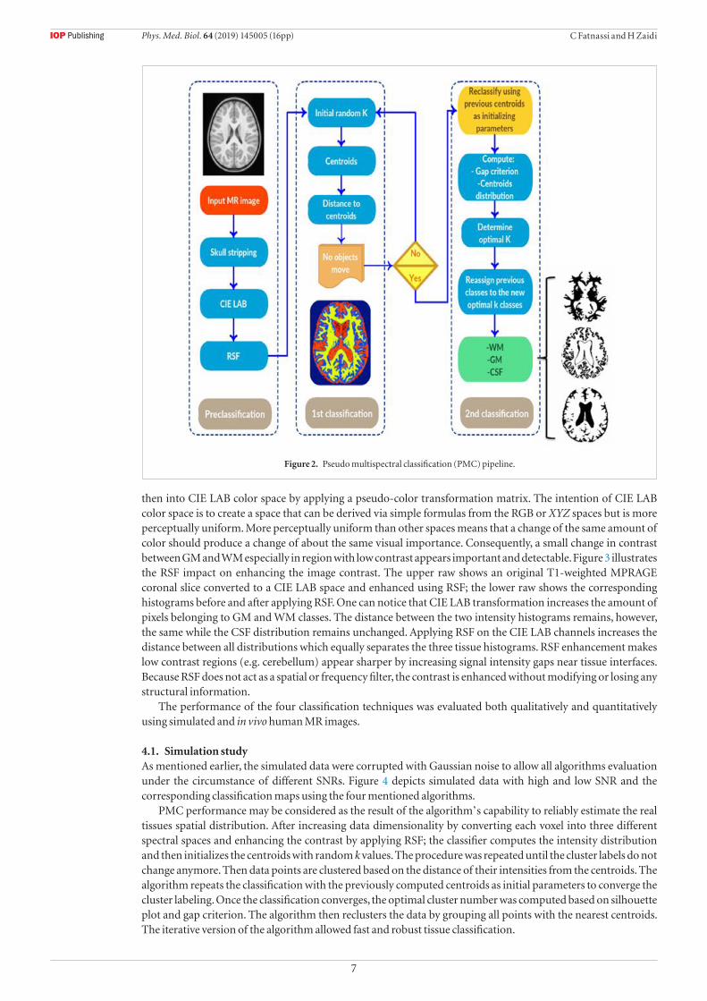
then into CIE LAB color space by applying a pseudo-color transformation matrix. The intention of CIE LAB color space is to create a space that can be derived via simple formulas from the RGB or XYZ spaces but is more perceptually uniform. More perceptually uniform than other spaces means that a change of the same amount of color should produce a change of about the same visual importance. Consequently, a small change in contrast between GM and WM especially in region with low contrast appears important and detectable. Figure 3 illustrates the RSF impact on enhancing the image contrast. The upper raw shows an original T1-weighted MPRAGE coronal slice converted to a CIE LAB space and enhanced using RSF; the lower raw shows the corresponding histograms before and after applying RSF. One can notice that CIE LAB transformation increases the amount of pixels belonging to GM and WM classes. The distance between the two intensity histograms remains, however, the same while the CSF distribution remains unchanged. Applying RSF on the CIE LAB channels increases the distance between all distributions which equally separates the three tissue histograms. RSF enhancement makes low contrast regions (e.g. cerebellum) appear sharper by increasing signal intensity gaps near tissue interfaces. Because RSF does not act as a spatial or frequency filter, the contrast is enhanced without modifying or losing any structural information.

The performance of the four classification techniques was evaluated both qualitatively and quantitatively using simulated and in vivo human MR images.

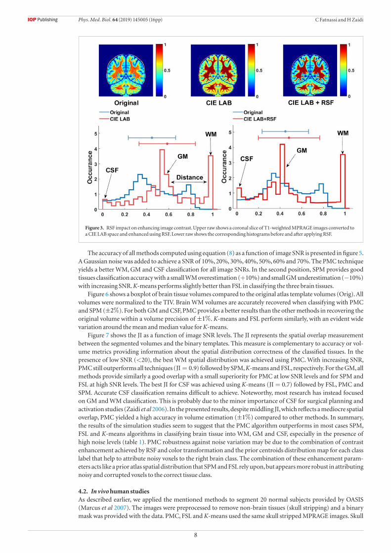
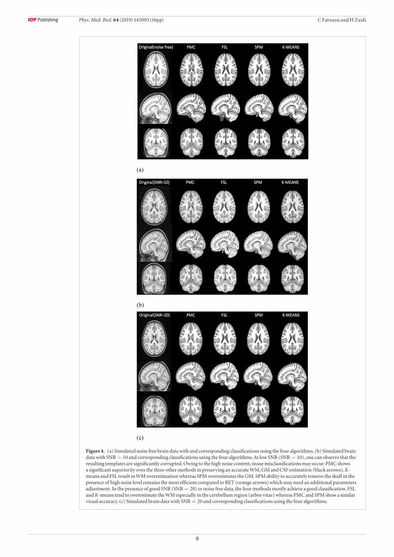
4.1. Simulation studyAs mentioned earlier, the simulated data were corrupted with Gaussian noise to allow all algorithms evaluation under the circumstance of different SNRs. Figure 4 depicts simulated data with high and low SNR and the corresponding classification maps using the four mentioned algorithms.

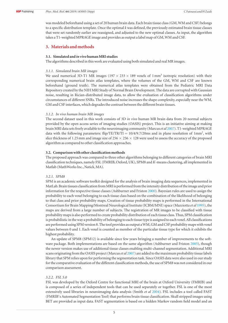
PMC performance may be considered as the result of the algorithm’s capability to reliably estimate the real tissues spatial distribution. After increasing data dimensionality by converting each voxel into three different spectral spaces and enhancing the contrast by applying RSF; the classifier computes the intensity distribution and then initializes the centroids with random k values. The procedure was repeated until the cluster labels do not change anymore. Then data points are clustered based on the distance of their intensities from the centroids. The algorithm repeats the classification with the previously computed centroids as initial parameters to converge the cluster labeling. Once the classification converges, the optimal cluster number was computed based on silhouette plot and gap criterion. The algorithm then reclusters the data by grouping all points with the nearest centroids. The iterative version of the algorithm allowed fast and robust tissue classification.

Figure 2. Pseudo multispectral classification (PMC) pipeline.

Phys. Med. Biol. 64 (2019) 145005 (16pp)

8

C Fatnassi and H Zaidi

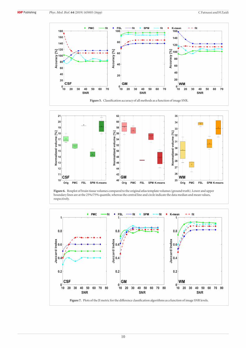
The accuracy of all methods computed using equation (8) as a function of image SNR is presented in figure 5. A Gaussian noise was added to achieve a SNR of 10%, 20%, 30%, 40%, 50%, 60% and 70%. The PMC technique yields a better WM, GM and CSF classification for all image SNRs. In the second position, SPM provides good tissues classification accuracy with a small WM overestimation (+10%) and small GM underestimation (−10%) with increasing SNR. K-means performs slightly better than FSL in classifying the three brain tissues.

Figure 6 shows a boxplot of brain tissue volumes compared to the original atlas template volumes (Orig). All volumes were normalized to the TIV. Brain WM volumes are accurately recovered when classifying with PMC and SPM (±2%). For both GM and CSF, PMC provides a better results than the other methods in recovering the original volume within a volume precision of ±1%. K-means and FSL perform similarly, with an evident wide variation around the mean and median value for K-means.

Figure 7 shows the JI as a function of image SNR levels. The JI represents the spatial overlap measurement between the segmented volumes and the binary templates. This measure is complementary to accuracy or vol-ume metrics providing information about the spatial distribution correctness of the classified tissues. In the presence of low SNR (<20), the best WM spatial distribution was achieved using PMC. With increasing SNR, PMC still outperforms all techniques (JI = 0.9) followed by SPM, K-means and FSL, respectively. For the GM, all methods provide similarly a good overlap with a small superiority for PMC at low SNR levels and for SPM and FSL at high SNR levels. The best JI for CSF was achieved using K-means (JI = 0.7) followed by FSL, PMC and SPM. Accurate CSF classification remains difficult to achieve. Noteworthy, most research has instead focused on GM and WM classification. This is probably due to the minor importance of CSF for surgical planning and activation studies (Zaidi et al 2006). In the presented results, despite middling JI, which reflects a mediocre spatial overlap, PMC yielded a high accuracy in volume estimation (±1%) compared to other methods. In summary, the results of the simulation studies seem to suggest that the PMC algorithm outperforms in most cases SPM, FSL and K-means algorithms in classifying brain tissue into WM, GM and CSF, especially in the presence of high noise levels (table 1). PMC robustness against noise variation may be due to the combination of contrast enhancement achieved by RSF and color transformation and the prior centroids distribution map for each class label that help to attribute noisy voxels to the right brain class. The combination of these enhancement param-eters acts like a prior atlas spatial distribution that SPM and FSL rely upon, but appears more robust in attributing noisy and corrupted voxels to the correct tissue class.

4.2. In vivo human studiesAs described earlier, we applied the mentioned methods to segment 20 normal subjects provided by OASIS (Marcus et al 2007). The images were preprocessed to remove non-brain tissues (skull stripping) and a binary mask was provided with the data. PMC, FSL and K-means used the same skull stripped MPRAGE images. Skull

Figure 3. RSF impact on enhancing image contrast. Upper raw shows a coronal slice of T1-weighted MPRAGE images converted to a CIE LAB space and enhanced using RSF. Lower raw shows the corresponding histograms before and after applying RSF.

Phys. Med. Biol. 64 (2019) 145005 (16pp)

9

C Fatnassi and H Zaidi

Figure 4. (a) Simulated noise free brain data with and corresponding classifications using the four algorithms. (b) Simulated brain data with SNR = 10 and corresponding classifications using the four algorithms. At low SNR (SNR = 10), one can observe that the resulting templates are significantly corrupted. Owing to the high noise content, tissue misclassifications may occur. PMC shows a significant superiority over the three other methods in preserving an accurate WM, GM and CSF estimation (black arrows). K-means and FSL result in WM overestimation whereas SPM overestimates the GM. SPM ability to accurately remove the skull in the presence of high noise level remains the most efficient compared to BET (orange arrows) which may need an additional parameters adjustment. In the presence of good SNR (SNR = 20) or noise free data, the four methods mostly achieve a good classification. FSL and K-means tend to overestimate the WM especially in the cerebellum region (arbor vitae) whereas PMC and SPM show a similar visual accuracy. (c) Simulated brain data with SNR = 20 and corresponding classifications using the four algorithms.

Phys. Med. Biol. 64 (2019) 145005 (16pp)

10

C Fatnassi and H Zaidi

Figure 5. Classification accuracy of all methods as a function of image SNR.

Figure 6. Boxplot of brain tissue volumes compared to the original atlas template volumes (ground truth). Lower and upper boundary lines are at the 25%/75% quantile, whereas the central line and circle indicate the data median and mean values, respectively.

Figure 7. Plots of the JI metric for the difference classification algorithms as a function of image SNR levels.

Phys. Med. Biol. 64 (2019) 145005 (16pp)

11

C Fatnassi and H Zaidi

stripping in SPM can be performed by segmenting the anatomical image, and using a thresholded version of the sum of grey and WM probability maps to mask out the non-intracranial tissue (Boesen et al 2004).

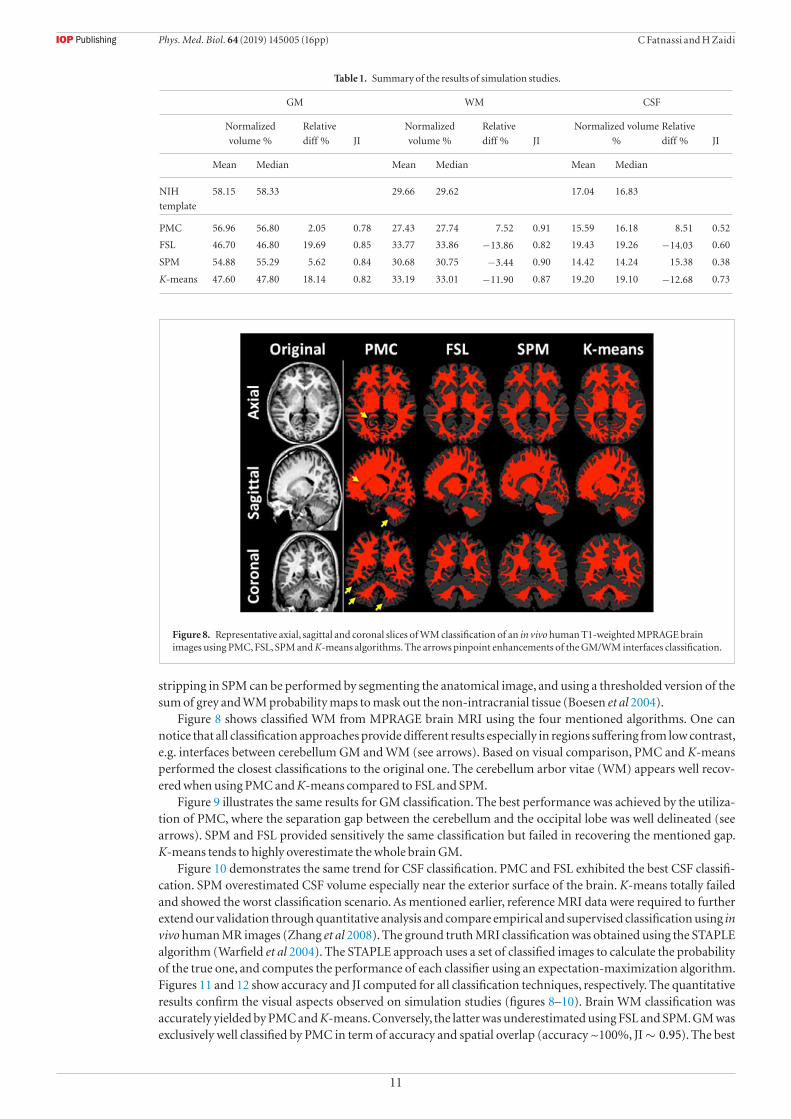
Figure 8 shows classified WM from MPRAGE brain MRI using the four mentioned algorithms. One can notice that all classification approaches provide different results especially in regions suffering from low contrast, e.g. interfaces between cerebellum GM and WM (see arrows). Based on visual comparison, PMC and K-means performed the closest classifications to the original one. The cerebellum arbor vitae (WM) appears well recov-ered when using PMC and K-means compared to FSL and SPM.

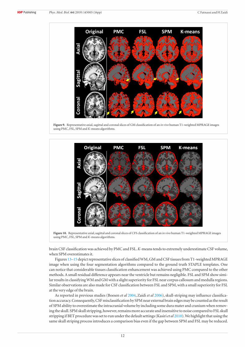
Figure 9 illustrates the same results for GM classification. The best performance was achieved by the utiliza-tion of PMC, where the separation gap between the cerebellum and the occipital lobe was well delineated (see arrows). SPM and FSL provided sensitively the same classification but failed in recovering the mentioned gap. K-means tends to highly overestimate the whole brain GM.

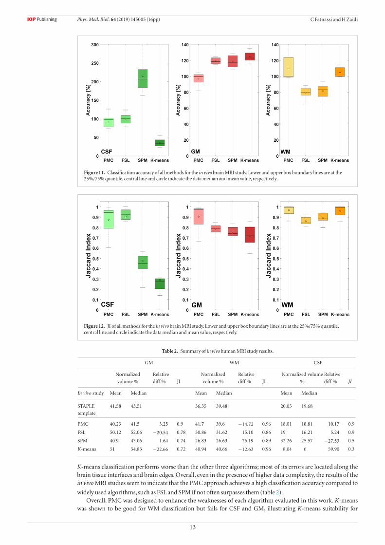
Figure 10 demonstrates the same trend for CSF classification. PMC and FSL exhibited the best CSF classifi-cation. SPM overestimated CSF volume especially near the exterior surface of the brain. K-means totally failed and showed the worst classification scenario. As mentioned earlier, reference MRI data were required to further extend our validation through quantitative analysis and compare empirical and supervised classification using in vivo human MR images (Zhang et al 2008). The ground truth MRI classification was obtained using the STAPLE algorithm (Warfield et al 2004). The STAPLE approach uses a set of classified images to calculate the probability of the true one, and computes the performance of each classifier using an expectation-maximization algorithm. Figures 11 and 12 show accuracy and JI computed for all classification techniques, respectively. The quantitative results confirm the visual aspects observed on simulation studies (figures 8–10). Brain WM classification was accurately yielded by PMC and K-means. Conversely, the latter was underestimated using FSL and SPM. GM was exclusively well classified by PMC in term of accuracy and spatial overlap (accuracy ~100%, JI ∼ 0.95). The best

Table 1. Summary of the results of simulation studies.

GM WM CSF

Normalized

volume %

Relative

diff % JI

Normalized

volume %

Relative

diff % JI

Normalized volume

%

Relative

diff % JI

Mean Median Mean Median Mean Median

NIH

template

58.15 58.33 29.66 29.62 17.04 16.83

PMC 56.96 56.80 2.05 0.78 27.43 27.74 7.52 0.91 15.59 16.18 8.51 0.52

FSL 46.70 46.80 19.69 0.85 33.77 33.86 −13.86 0.82 19.43 19.26 −14.03 0.60

SPM 54.88 55.29 5.62 0.84 30.68 30.75 −3.44 0.90 14.42 14.24 15.38 0.38

K-means 47.60 47.80 18.14 0.82 33.19 33.01 −11.90 0.87 19.20 19.10 −12.68 0.73

Figure 8. Representative axial, sagittal and coronal slices of WM classification of an in vivo human T1-weighted MPRAGE brain images using PMC, FSL, SPM and K-means algorithms. The arrows pinpoint enhancements of the GM/WM interfaces classification.

Phys. Med. Biol. 64 (2019) 145005 (16pp)

12

C Fatnassi and H Zaidi

brain CSF classification was achieved by PMC and FSL. K-means tends to extremely underestimate CSF volume, when SPM overestimates it.

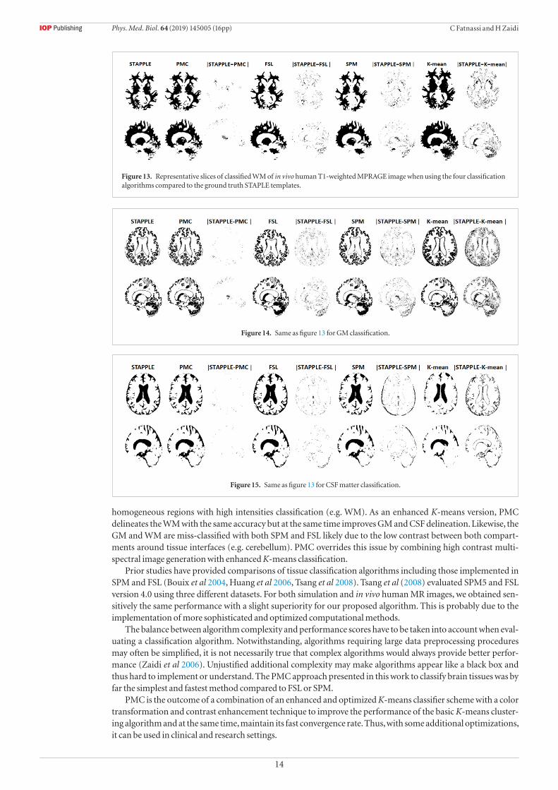
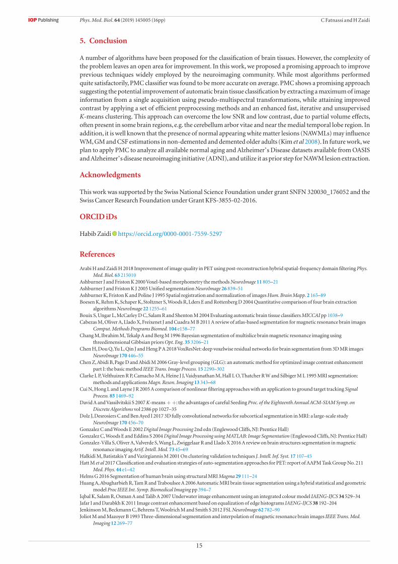
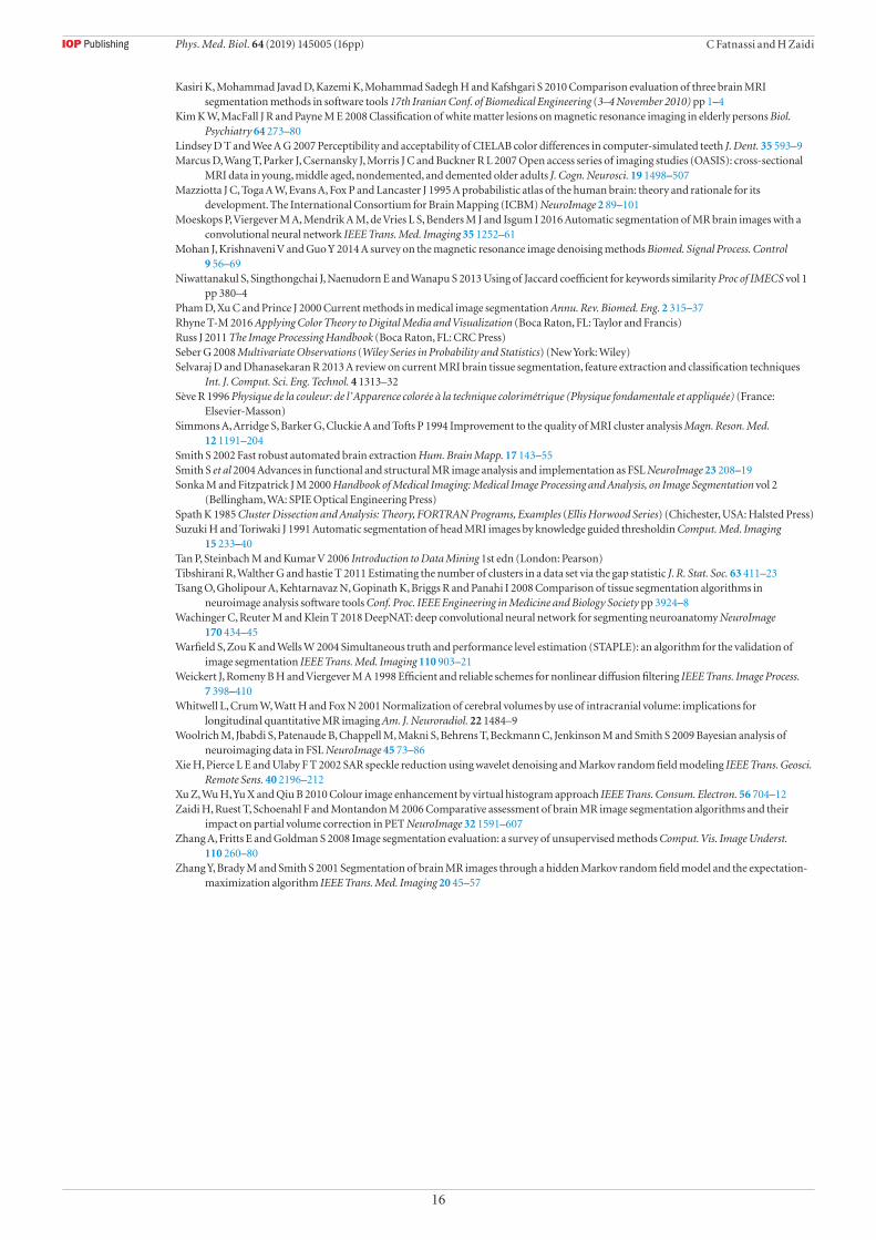
Figures 13–15 depict representative slices of classified WM, GM and CSF tissues from T1-weighted MPRAGE image when using the four segmentation algorithms compared to the ground truth STAPLE templates. One can notice that considerable tissues classification enhancement was achieved using PMC compared to the other methods. A small residual difference appears near the ventricle but remains negligible. FSL and SPM show simi-lar results in classifying WM and GM with a slight superiority for FSL near corpus callosum and medulla regions. Similar observations are also made for CSF classification between FSL and SPM, with a small superiority for FSL at the very edge of the brain.

As reported in previous studies (Boesen et al 2004, Zaidi et al 2006), skull-striping may influence classifica-tion accuracy. Consequently, CSF misclassification by SPM near external brain edges may be counted as the result of SPM ability to overestimate the intracranial volume by including some dura mater and cranium when remov-ing the skull. SPM skull stripping, however, remains more accurate and insensitive to noise compared to FSL skull stripping if BET procedure was set to run under the default settings (Kasiri et al 2010). We highlight that using the same skull striping process introduces a comparison bias even if the gap between SPM and FSL may be reduced.

Figure 9. Representative axial, sagittal and coronal slices of GM classification of an in vivo human T1-weighted MPRAGE images using PMC, FSL, SPM and K-means algorithms.

Figure 10. Representative axial, sagittal and coronal slices of CFS classification of an in vivo human T1-weighted MPRAGE images using PMC, FSL, SPM and K-means algorithms.

Phys. Med. Biol. 64 (2019) 145005 (16pp)

13

C Fatnassi and H Zaidi

K-means classification performs worse than the other three algorithms; most of its errors are located along the brain tissue interfaces and brain edges. Overall, even in the presence of higher data complexity, the results of the in vivo MRI studies seem to indicate that the PMC approach achieves a high classification accuracy compared to

widely used algorithms, such as FSL and SPM if not often surpasses them (table 2).Overall, PMC was designed to enhance the weaknesses of each algorithm evaluated in this work. K-means

was shown to be good for WM classification but fails for CSF and GM, illustrating K-means suitability for

Figure 11. Classification accuracy of all methods for the in vivo brain MRI study. Lower and upper box boundary lines are at the 25%/75% quantile, central line and circle indicate the data median and mean value, respectively.

Figure 12. JI of all methods for the in vivo brain MRI study. Lower and upper box boundary lines are at the 25%/75% quantile, central line and circle indicate the data median and mean value, respectively.

Table 2. Summary of in vivo human MRI study results.

GM WM CSF

Normalized

volume %

Relative

diff % JI

Normalized

volume %

Relative

diff % JI

Normalized volume

%

Relative

diff % JI

In vivo study Mean Median Mean Median Mean Median

STAPLE

template

41.58 43.51 36.35 39.48 20.05 19.68

PMC 40.23 41.5 3.25 0.9 41.7 39.6 −14.72 0.96 18.01 18.81 10.17 0.9

FSL 50.12 52.06 −20.54 0.78 30.86 31.62 15.10 0.86 19 16.21 5.24 0.9

SPM 40.9 43.06 1.64 0.74 26.83 26.63 26.19 0.89 32.26 25.57 −27.53 0.5

K-means 51 54.83 −22.66 0.72 40.94 40.66 −12.63 0.96 8.04 6 59.90 0.3

Phys. Med. Biol. 64 (2019) 145005 (16pp)

14

C Fatnassi and H Zaidi

homogeneous regions with high intensities classification (e.g. WM). As an enhanced K-means version, PMC delineates the WM with the same accuracy but at the same time improves GM and CSF delineation. Likewise, the GM and WM are miss-classified with both SPM and FSL likely due to the low contrast between both compart-ments around tissue interfaces (e.g. cerebellum). PMC overrides this issue by combining high contrast multi-spectral image generation with enhanced K-means classification.

Prior studies have provided comparisons of tissue classification algorithms including those implemented in SPM and FSL (Bouix et al 2004, Huang et al 2006, Tsang et al 2008). Tsang et al (2008) evaluated SPM5 and FSL version 4.0 using three different datasets. For both simulation and in vivo human MR images, we obtained sen-sitively the same performance with a slight superiority for our proposed algorithm. This is probably due to the implementation of more sophisticated and optimized computational methods.

The balance between algorithm complexity and performance scores have to be taken into account when eval-uating a classification algorithm. Notwithstanding, algorithms requiring large data preprocessing procedures may often be simplified, it is not necessarily true that complex algorithms would always provide better perfor-mance (Zaidi et al 2006). Unjustified additional complexity may make algorithms appear like a black box and thus hard to implement or understand. The PMC approach presented in this work to classify brain tissues was by far the simplest and fastest method compared to FSL or SPM.

PMC is the outcome of a combination of an enhanced and optimized K-means classifier scheme with a color transformation and contrast enhancement technique to improve the performance of the basic K-means cluster-ing algorithm and at the same time, maintain its fast convergence rate. Thus, with some additional optimizations, it can be used in clinical and research settings.

Figure 13. Representative slices of classified WM of in vivo human T1-weighted MPRAGE image when using the four classification algorithms compared to the ground truth STAPLE templates.

Figure 14. Same as figure 13 for GM classification.

Figure 15. Same as figure 13 for CSF matter classification.

Phys. Med. Biol. 64 (2019) 145005 (16pp)

15

C Fatnassi and H Zaidi

5. Conclusion

A number of algorithms have been proposed for the classification of brain tissues. However, the complexity of the problem leaves an open area for improvement. In this work, we proposed a promising approach to improve previous techniques widely employed by the neuroimaging community. While most algorithms performed quite satisfactorily, PMC classifier was found to be more accurate on average. PMC shows a promising approach suggesting the potential improvement of automatic brain tissue classification by extracting a maximum of image information from a single acquisition using pseudo-multispectral transformations, while attaining improved contrast by applying a set of efficient preprocessing methods and an enhanced fast, iterative and unsupervised K-means clustering. This approach can overcome the low SNR and low contrast, due to partial volume effects, often present in some brain regions, e.g. the cerebellum arbor vitae and near the medial temporal lobe region. In addition, it is well known that the presence of normal appearing white matter lesions (NAWMLs) may influence WM, GM and CSF estimations in non-demented and demented older adults (Kim et al 2008). In future work, we plan to apply PMC to analyze all available normal aging and Alzheimer’s Disease datasets available from OASIS and Alzheimer’s disease neuroimaging initiative (ADNI), and utilize it as prior step for NAWM lesion extraction.

Acknowledgments

This work was supported by the Swiss National Science Foundation under grant SNFN 320030_176052 and the Swiss Cancer Research Foundation under Grant KFS-3855-02-2016.

ORCID iDs

Habib Zaidi https://orcid.org/0000-0001-7559-5297

References

Arabi H and Zaidi H 2018 Improvement of image quality in PET using post-reconstruction hybrid spatial-frequency domain filtering Phys. Med. Biol. 63 215010

Ashburner J and Friston K 2000 Voxel-based morphometry the methods NeuroImage 11 805–21Ashburner J and Friston K J 2005 Unified segmentation NeuroImage 26 839–51Ashburner K, Friston K and Poline J 1995 Spatial registration and normalization of images Hum. Brain Mapp. 2 165–89Boesen K, Rehm K, Schaper K, Stoltzner S, Woods R, Lders E and Rottenberg D 2004 Quantitative comparison of four brain extraction

algorithms NeuroImage 22 1255–61Bouix S, Ungar L, McCarley D C, Salam R and Shenton M 2004 Evaluating automatic brain tissue classifiers MICCAI pp 1038–9Cabezas M, Oliver A, Llado X, Freixenet J and Cuadra M B 2011 A review of atlas-based segmentation for magnetic resonance brain images

Comput. Methods Programs Biomed. 104 e158–77Chang M, Ibrahim M, Tekalp A and Berg M 1996 Bayesian segmentation of multislice brain magnetic resonance imaging using

threedimensional Gibbsian priors Opt. Eng. 35 3206–21Chen H, Dou Q, Yu L, Qin J and Heng P A 2018 VoxResNet: deep voxelwise residual networks for brain segmentation from 3D MR images

NeuroImage 170 446–55Chen Z, Abidi B, Page D and Abidi M 2006 Gray-level grouping (GLG): an automatic method for optimized image contrast enhancement

part I: the basic method IEEE Trans. Image Process. 15 2290–302Clarke L P, Velthuizen R P, Camacho M A, Heine J J, Vaidyanathan M, Hall L O, Thatcher R W and Silbiger M L 1995 MRI segmentation:

methods and applications Magn. Reson. Imaging 13 343–68Cui N, Hong L and Layne J R 2005 A comparison of nonlinear filtering approaches with an application to ground target tracking Signal

Process. 85 1469–92David A and Vassilvitskii S 2007 K-means + +: the advantages of careful Seeding Proc. of the Eighteenth Annual ACM-SIAM Symp. on

Discrete Algorithms vol 2386 pp 1027–35Dolz J, Desrosiers C and Ben Ayed I 2017 3D fully convolutional networks for subcortical segmentation in MRI: a large-scale study

NeuroImage 170 456–70Gonzalez C and Woods E 2002 Digital Image Processing 2nd edn (Englewood Cliffs, NJ: Prentice Hall)Gonzalez C, Woods E and Eddins S 2004 Digital Image Processing using MATLAB: Image Segmentation (Englewood Cliffs, NJ: Prentice Hall)Gonzalez-Villa S, Oliver A, Valverde S, Wang L, Zwiggelaar R and Llado X 2016 A review on brain structures segmentation in magnetic

resonance imaging Artif. Intell. Med. 73 45–69Halkidi M, Batistakis Y and Vazirgiannis M 2001 On clustering validation techniques J. Intell. Inf. Syst. 17 107–45Hatt M et al 2017 Classification and evaluation strategies of auto-segmentation approaches for PET: report of AAPM Task Group No. 211

Med. Phys. 44 e1–42Helms G 2016 Segmentation of human brain using structural MRI Magma 29 111–24Huang A, Abugharbieh R, Tam R and Traboulsee A 2006 Automatic MRI brain tissue segmentation using a hybrid statistical and geometric

model Proc IEEE Int. Symp. Biomedical Imaging pp 394–7Iqbal K, Salam R, Osman A and Talib A 2007 Underwater image enhancement using an integrated colour model IAENG-IJCS 34 529–34Jafar I and Darabkh K 2011 Image contrast enhancement based on equalization of edge histograms IAENG-IJCS 38 192–204Jenkinson M, Beckmann C, Behrens T, Woolrich M and Smith S 2012 FSL NeuroImage 62 782–90Joliot M and Mazoyer B 1993 Three-dimensional segmentation and interpolation of magnetic resonance brain images IEEE Trans. Med.

Imaging 12 269–77

Phys. Med. Biol. 64 (2019) 145005 (16pp)

16

C Fatnassi and H Zaidi

Kasiri K, Mohammad Javad D, Kazemi K, Mohammad Sadegh H and Kafshgari S 2010 Comparison evaluation of three brain MRI segmentation methods in software tools 17th Iranian Conf. of Biomedical Engineering (3–4 November 2010) pp 1–4

Kim K W, MacFall J R and Payne M E 2008 Classification of white matter lesions on magnetic resonance imaging in elderly persons Biol. Psychiatry 64 273–80

Lindsey D T and Wee A G 2007 Perceptibility and acceptability of CIELAB color differences in computer-simulated teeth J. Dent. 35 593–9Marcus D, Wang T, Parker J, Csernansky J, Morris J C and Buckner R L 2007 Open access series of imaging studies (OASIS): cross-sectional

MRI data in young, middle aged, nondemented, and demented older adults J. Cogn. Neurosci. 19 1498–507Mazziotta J C, Toga A W, Evans A, Fox P and Lancaster J 1995 A probabilistic atlas of the human brain: theory and rationale for its

development. The International Consortium for Brain Mapping (ICBM) NeuroImage 2 89–101Moeskops P, Viergever M A, Mendrik A M, de Vries L S, Benders M J and Isgum I 2016 Automatic segmentation of MR brain images with a

convolutional neural network IEEE Trans. Med. Imaging 35 1252–61Mohan J, Krishnaveni V and Guo Y 2014 A survey on the magnetic resonance image denoising methods Biomed. Signal Process. Control

9 56–69Niwattanakul S, Singthongchai J, Naenudorn E and Wanapu S 2013 Using of Jaccard coefficient for keywords similarity Proc of IMECS vol 1

pp 380–4Pham D, Xu C and Prince J 2000 Current methods in medical image segmentation Annu. Rev. Biomed. Eng. 2 315–37Rhyne T-M 2016 Applying Color Theory to Digital Media and Visualization (Boca Raton, FL: Taylor and Francis)Russ J 2011 The Image Processing Handbook (Boca Raton, FL: CRC Press)Seber G 2008 Multivariate Observations (Wiley Series in Probability and Statistics) (New York: Wiley) Selvaraj D and Dhanasekaran R 2013 A review on current MRI brain tissue segmentation, feature extraction and classification techniques

Int. J. Comput. Sci. Eng. Technol. 4 1313–32Sève R 1996 Physique de la couleur: de l’Apparence colorée à la technique colorimétrique (Physique fondamentale et appliquée) (France:

Elsevier-Masson) Simmons A, Arridge S, Barker G, Cluckie A and Tofts P 1994 Improvement to the quality of MRI cluster analysis Magn. Reson. Med.

12 1191–204Smith S 2002 Fast robust automated brain extraction Hum. Brain Mapp. 17 143–55Smith S et al 2004 Advances in functional and structural MR image analysis and implementation as FSL NeuroImage 23 208–19Sonka M and Fitzpatrick J M 2000 Handbook of Medical Imaging: Medical Image Processing and Analysis, on Image Segmentation vol 2

(Bellingham, WA: SPIE Optical Engineering Press)Spath K 1985 Cluster Dissection and Analysis: Theory, FORTRAN Programs, Examples (Ellis Horwood Series) (Chichester, USA: Halsted Press)Suzuki H and Toriwaki J 1991 Automatic segmentation of head MRI images by knowledge guided thresholdin Comput. Med. Imaging

15 233–40Tan P, Steinbach M and Kumar V 2006 Introduction to Data Mining 1st edn (London: Pearson)Tibshirani R, Walther G and hastie T 2011 Estimating the number of clusters in a data set via the gap statistic J. R. Stat. Soc. 63 411–23Tsang O, Gholipour A, Kehtarnavaz N, Gopinath K, Briggs R and Panahi I 2008 Comparison of tissue segmentation algorithms in

neuroimage analysis software tools Conf. Proc. IEEE Engineering in Medicine and Biology Society pp 3924–8Wachinger C, Reuter M and Klein T 2018 DeepNAT: deep convolutional neural network for segmenting neuroanatomy NeuroImage

170 434–45Warfield S, Zou K and Wells W 2004 Simultaneous truth and performance level estimation (STAPLE): an algorithm for the validation of

image segmentation IEEE Trans. Med. Imaging 110 903–21Weickert J, Romeny B H and Viergever M A 1998 Efficient and reliable schemes for nonlinear diffusion filtering IEEE Trans. Image Process.

7 398–410Whitwell L, Crum W, Watt H and Fox N 2001 Normalization of cerebral volumes by use of intracranial volume: implications for

longitudinal quantitative MR imaging Am. J. Neuroradiol. 22 1484–9Woolrich M, Jbabdi S, Patenaude B, Chappell M, Makni S, Behrens T, Beckmann C, Jenkinson M and Smith S 2009 Bayesian analysis of

neuroimaging data in FSL NeuroImage 45 73–86Xie H, Pierce L E and Ulaby F T 2002 SAR speckle reduction using wavelet denoising and Markov random field modeling IEEE Trans. Geosci.

Remote Sens. 40 2196–212Xu Z, Wu H, Yu X and Qiu B 2010 Colour image enhancement by virtual histogram approach IEEE Trans. Consum. Electron. 56 704–12Zaidi H, Ruest T, Schoenahl F and Montandon M 2006 Comparative assessment of brain MR image segmentation algorithms and their

impact on partial volume correction in PET NeuroImage 32 1591–607Zhang A, Fritts E and Goldman S 2008 Image segmentation evaluation: a survey of unsupervised methods Comput. Vis. Image Underst.

110 260–80Zhang Y, Brady M and Smith S 2001 Segmentation of brain MR images through a hidden Markov random field model and the expectation-

maximization algorithm IEEE Trans. Med. Imaging 20 45–57

Phys. Med. Biol. 64 (2019) 145005 (16pp)