Fast and accurate position control of shape memory alloy...

Département EEA, M1 P-IST Robotic systems lab

2008

Fast and accurate position

control of shape memory

alloy actuators

Internship report, first year of master degree

Sylvain Toru

I. Introduction

Research internship report 2008 | Sylvain Toru

TABLE OF C ONTEN TS

Introduction..................................................................................................................................... 4

1. Context of the internship ...................................................................................................... 4

2. Why shape memory alloy actuators? ..................................................................................... 4

3. Internship objectives............................................................................................................. 5

4. Report outline ...................................................................................................................... 6

Abstract in French / Résumé long en Français ................................................................................... 7

Shape memory alloys ....................................................................................................................... 8

1. What is a shape memory alloy............................................................................................... 8

2. The shape memory effect ..................................................................................................... 8

3. SMA actuators .................................................................................................................... 10

The test bed................................................................................................................................... 12

1. The power amplifier............................................................................................................ 13

2. The load cells ...................................................................................................................... 19

3. The linear slide ................................................................................................................... 20

4. Safety features ................................................................................................................... 23

Differential force control of antagonistic SMA actuators ................................................................. 24

1. Control architecture............................................................................................................ 24

2. The controller ..................................................................................................................... 24

3. The anti-slack mechanism ................................................................................................... 26

4. The rapid-heating mechanism ............................................................................................. 27

5. The anti-overload mechanism ............................................................................................. 31

6. Results with disturbances.................................................................................................... 32

Stiffness Control of antagonistic SMA actuators .............................................................................. 34

1. Objectives .......................................................................................................................... 34

I. Introduction


2. The design .......................................................................................................................... 34

3. Results ............................................................................................................................... 34

Position control of antagonistic SMA actuators ............................................................................... 39

1. Objectives .......................................................................................................................... 39

2. The design .......................................................................................................................... 39

3. Results ............................................................................................................................... 39

Conclusions.................................................................................................................................... 42

Appendix: Simulink models............................................................................................................. 43

Cited works.................................................................................................................................... 53

I. Introduction


I. INTRO DUCTION

1. CONTEXT OF THE INTERNSHIP

Figure 1 - RSISE building

To conclude the first year of my master degree in electrical engineering and applied

physics, I had the luck to do my internship in the Robotic systems Lab, in the Research School

of Information Science and Engineering (RSISE) of the Australian National University (ANU) in

Canberra, Australia. This lab is part of the Information Engineering Department, headed by

Prof. Rod Kennedy. In this department, over 100 active researchers work on four main

research groups: applied signal processing, computer vision, systems and control and

robotics.

I worked two months in this last group, supervised by Dr. Roy Featherstone who I truly

want to thank for having invited me in his lab! This project is the result of the work of Yee

Harn Teh, who studied SMA during his Honours degree (1) and his PhD (2). He managed to

build a model of the SMA actuator and achieved a fast and accurate differential force

controller. He also worked on a position controller.

2. WHY S HAPE MEMORY ALLOY ACTUATORS?

Many systems depend on actuators which are their driving systems. Usually, those

actuators use electric, hydraulic or pneumatic technologies. Since we need systems more

and more compact, we also need to consider new actuators, such as piezoelectrics or shape

memory alloy actuators.

Shape memory alloy wires can be easily stretched when they are cold but they return

forcefully to their initial length when heated (by Joule effect for example). Although they are

very difficult to control and they have a slow response speed, they have a great potential in

niche applications where space, weight, cost and noise are crucial factors. Indeed, a pair of

antagonistic SMA wire can lift a weight of 1000 times its proper weight when heated.

I. Introduction


Moreover, an actuator of this kind can be very compact since it is composed of only two thin

wires, and no reduction gear system is needed, like for an electric motor. Last, those

actuators are clean (no oil needed to maintain it, no dust is produced), silent, and spark free.

That makes them very suitable for microelectronics or medical applications.

Of course, they are not free from dra wbacks. Indeed, they have very low energy

efficiency. According to J.Van Humbeeck(3), the maximum theoretical efficiency is of the

order of 10% but in reality, it is hardly 1%. That means most of the heating energy is lost to

the air. This makes those kinds of actuators really interesting where energy efficiency is less

important than properties like weight, size, and so on. The SMA actuators can suffer from

fatigue if they are frequently overstressed or overstrained. Thus a special care should be

taken to prevent this from happening. However, commercially available SMA wires, such as

Flexinol, are trained to achieve several millions of cycles without losing the shape memory

effect. Finally, SMA actuators are very slow and inaccurate and the large hysteresis

transformation loop makes them difficult to control. Most of the control research aims to

solve this problem.

As a result, if well controlled, actuators made with those thin wires of SMA could replace

some bigger ones for example in surgery when miniature devices are required: little video

cameras for endoscopy, precisions tools, and so on. For now, SMA actuators remain mostly

as experimental actuators because of the difficulty of controlling them.

3. INTERNSHIP OBJECTIVES

As said previously, the SMA actuators are very difficult to control. This kind of material is

highly non linear and attempts to control them in the presence of an external load usually

result in limit cycles. This problem has been pursued by various researchers but never fully

solved. However, Yee Harn Teh managed to control an actuator made of a pair of

antagonistic SMA wires without limit cycles happening. He aims to control the differential

force between the two SMA wires. The main control system of the differential force

controller is a high bandwidth PID controller. Other components are the anti-slack

mechanism, the rapid heating mechanism and the anti-overload mechanism. The result is a

closed loop fast and accurate, even in the presence of external motion disturbances.

Moreover, there is an outer loop to achieve position control with another PID controller.

For all the experiments on the test bed, a PC running Matlab/Simulink is used to program

and implement control systems on a dSPACE real-time control board. During my internship, I

first had to repeat Yee Harn’s experiments with new simulink models and to build a SMA

library with the main control systems. I also had to document them in order for the future

students who will be working on the test bed to handle it very quickly. Then, I had to

I. Introduction


program and test new control systems, first to build a stiffness controller and then to

improve the results in the field of the motion control.

4. REPORT O UTLINE

This report is organized in the following manner.

The following chapter is a long abstract of this report in French .

In Chapter III, some general pieces of information are given on those alloys. Then, the

shape memory effect is quickly described and we see why they are interesting for building

actuators, and how to build those actuators.

Chapter IV describes all the components of the experiment. That was the first part of my

work: make the plant work again. In order to do this, I had to use another power amplifier

than the original one, to calibrate the load cells and tune the controller of the linear slide on

which the SMA wires are attached. Then several safety features for the plant are described.

They are mainly implemented not to damage the SMA wires.

Chapter V is mainly about Yee Harn’s thesis. It describes all the mechanisms he invented

to improve the velocity and the accuracy in force control. The one and only difference is in

the anti-overload mechanism, which I implemented differently. The results he got with its

controller are also depicted in this chapter.

In Chapter VI, is described how I implemented the stiffness controller and what results I

got.

Finally, I explain in Chapter VII the modifications I made in the differential force

controller to make it a position controller. The results I got are also depicted in this chapter.

Please note that Figures 2, 5, 4, 18, 19, 20, 21, 22, 23, and 24 are drawn from Yee Harn’s

Honours (1) and phD (2) theses. Figures 3 and 16 are drawn from Dr Roy Featherstone slides

for a talk on SMA.

II. Abstract in French / Résumé long en Français


II. ABSTRACT IN FRENCH / RESUME LONG EN FRANÇAIS

III. Shape memory alloys


III. SHAPE MEM ORY A LLOYS

In this section, shape memory alloys and their different phases are explained as well as the

way of building a shape memory alloy actuator.

1. WHAT IS A S HAPE MEMORY ALLOY

Shape memory alloys are a group of metallic materials that are distinguished by their

ability to remember their shape. After a deformation and upon specific temperature and/or

stress conditions, they can recover their initial shape. Currently, those alloys are based on

NiTi (NiTi, NiTiCu, NiTiPd...), Cu (CuZn, CuZnAl, CuAlNiMn...) and Fe (FePt, FeMnSi, FeNiC...)

and the one used for our experiments is the NiTi. It has been called Flexinol by Dynalloy Inc.

which manufactures and markets it.

There are two main phases for those alloys: the martensite and the austenite phases.

When a SMA is in its martensite phase, it can easily be deformed to a new shape (obviously,

there are limits in the strain you impose to the material). Then, when the SMA is heated, it

can go to its austenite phase and recover its original shape. This transformation process is

called the shape memory effect and is the basis of this work on SMA actuators.

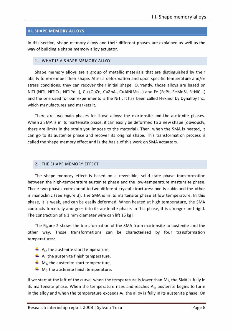
2. THE S HAPE MEMORY EFFECT

The shape memory effect is based on a reversible, solid-state phase transformation

between the high-temperature austenite phase and the low-temperature martensite phase.

Those two phases correspond to two different crystal structures: one is cubic and the other

is monoclinic (see Figure 3). The SMA is in its martensite phase at low temperature. In this

phase, it is weak, and can be easily deformed. When heated at high temperature, the SMA

contracts forcefully and goes into its austenite phase. In this phase, it is stronger and rigid.

The contraction of a 1 mm diameter wire can lift 15 kg!

The Figure 2 shows the transformation of the SMA from martensite to austenite and the

other way. Those transformations can be characterised by four transformation

temperatures:

As, the austenite start temperature,

Af, the austenite finish temperature,

Ms, the austenite start temperature,

Mf, the austenite finish temperature.

If we start at the left of the curve, when the temperature is lower than Mf, the SMA is fully in

its martensite phase. When the temperature rises and reaches As, austenite begins to form

in the alloy and when the temperature exceeds Af, the alloy is fully in its austenite phase. On



the way back, martensite begin to form when the temperature drops below Ms and the SMA

is again fully martensitic below Mf. This curve presents a wide hysteresis loop. Its width

varies with the alloy system. For NiTi alloys, the temperature hysteresis is usually between

30 and 50°C.Besides the common shape change effects such as elastic or thermal

deformations, SMAs present three shape memory characteristics:

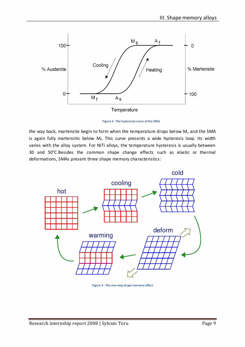
Figure 3 - The one-way shape memory effect

Figure 2 - The hysteresis curve of the SMA



The one-way shape memory effect: after the removal of an external force, the alloy

keeps its form due to the deformation. It can recover its initial shape upon heating,

and cooling does not affect its shape.

The two-ways memory effect: the shape change can also happen upon cooling,

without external stress.

Pseudo elasticity: at temperature beyond Af, stressing the SMA can drive it in a third

phase called stress-induced martensite. When the stress is removed, the alloy reverts

to its initial shape. During those transformations, no thermal process is involved.

This is the one-way shape memory effect that is the basis of SMA actuators. It is depicted in

the Figure 3. The red squares denote austenite crystals and blue parallelograms denote

martensite crystals.

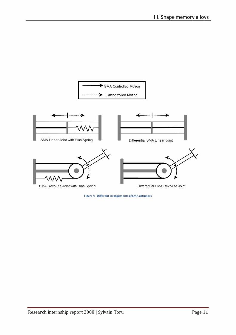
3. SMA ACTUATO RS

The shape memory alloys can contract to return to their initial shape. More, they

contract with a large strength. A SMA wire with a diameter of 1mm can lift a weight of 15kg.

Therefore, it has a very high force-to-weight ratio. Actually, SMAs show a work density of 107

Jm-3, which is 25 times greater than the work density of electrical motors (4).

As a result, SMA can be used to generate force and motion, used as actuators in various

configurations. One of them is SMA wires: heating them can easily be achieved by driving a

current through them. The Joule effect will do the rest. Obviously, the difficulty is to control

this temperature. Another problem is that because SMA wires use the one-way shape

memory effect, they can only contract in one direction, so it is necessary to provide a biasing

force to return to the neutral position. It can be provided by a spring or other SMA wires in

different arrangements, as shown in the Figure 4.

For our experiment, we use a rotating actuator, made of a pulley on which 2 wires are

connected, one on each side of the pulley. As a result, when one is being heated, the other is

being stretched. This solution is better than using a spring because you can control actively

the rotation of the pulley in both ways. More details on the test bed are given in the

following chapter.



Figure 4 - Different arrangements of SMA actuators

IV. The test bed


IV. THE TEST BED

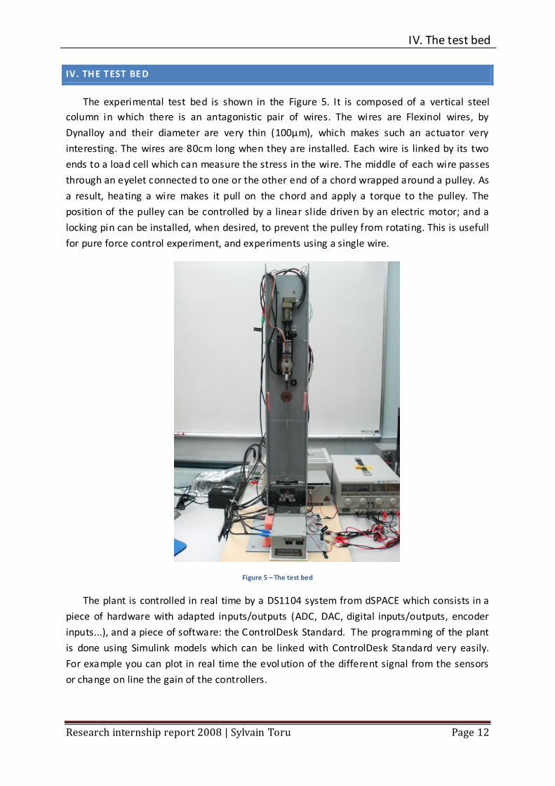
The experimental test bed is shown in the Figure 5. It is composed of a vertical steel

column in which there is an antagonistic pair of wires. The wires are Flexinol wires, by

Dynalloy and their diameter are very thin (100µm), which makes such an actuator very

interesting. The wires are 80cm long when they are installed. Each wire is linked by its two

ends to a load cell which can measure the stress in the wire. The middle of each wire passes

through an eyelet connected to one or the other end of a chord wrapped around a pulley. As

a result, heating a wire makes it pull on the chord and apply a torque to the pulley. The

position of the pulley can be controlled by a linear slide driven by an electric motor; and a

locking pin can be installed, when desired, to prevent the pulley from rotating. This is usefull

for pure force control experiment, and experiments using a single wire.

Figure 5 – The test bed

The plant is controlled in real time by a DS1104 system from dSPACE which consists in a

piece of hardware with adapted inputs/outputs (ADC, DAC, digital inputs/outputs, encoder

inputs...), and a piece of software: the ControlDesk Standard. The programming of the plant

is done using Simulink models which can be linked with ControlDesk Standard very easily.

For example you can plot in real time the evol ution of the different signal from the sensors

or change on line the gain of the controllers.

IV. The test bed


Before I arrived in the lab, the system was broken by the previous student who worked

on it. The power amplifier was broken and the load cells as well. New load cells were

ordered and I was given an older power amplifier. My first task was to fix the test bed, so it

could work again.

1. THE POWER A MPLIFIER

To control accurately current in the wires, a precision power amplifier is needed. Since

the one built by Yee Harn during his thesis was broken, I was given an older amplifier, the

one he used for his Honours degree. Here is the amplifier circuit:

Figure 6 - Amplifier circuit

This amplifier is commanded by the voltage coming from the DAC and is supposed to

drive a constant current into the SMA wire. Two output voltages are available: the voltage

across R5 which is proportional to the current in the SMA wire and the one across R7 which

is a tenth of the voltage across the SMA wire and R5. This amplifier was designed for another

experiment so there are four amplifier of this type available. Since we have only two SMA

wires to control, two channels are unused.

To use properly this amplifier, I firstly characterised it with a 47Ω power resistor whose

resistance was precisely known. I then used a ramp as the input and looked at the voltage

across R7. Without forgetting the voltage divider of the output and R5 which must be added

to 47Ω to calculate the output current, I was able to plot the voltage-input/current-output

IV. The test bed


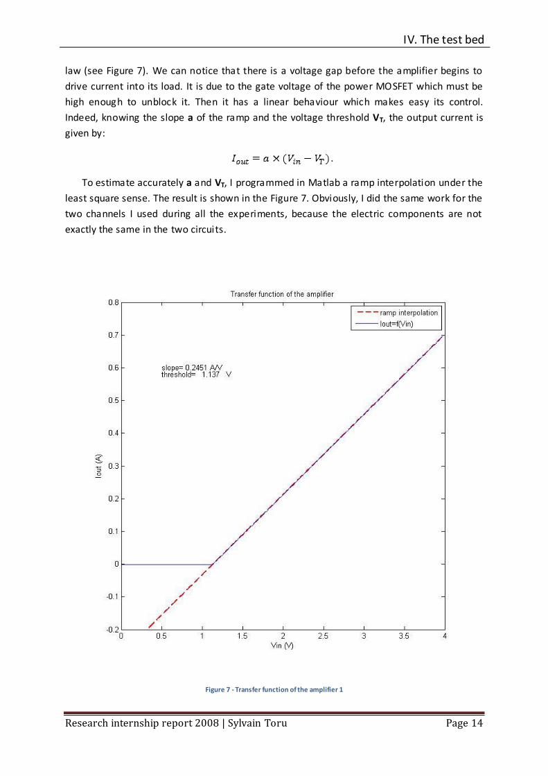
law (see Figure 7). We can notice that there is a voltage gap before the amplifier begins to

drive current into its load. It is due to the gate voltage of the power MOSFET which must be

high enough to unblock it. Then it has a linear behaviour which makes easy its control.

Indeed, knowing the slope a of the ramp and the voltage threshold VT, the output current is

given by:

.

To estimate accurately a and VT, I programmed in Matlab a ramp interpolation under the

least square sense. The result is shown in the Figure 7. Obviously, I did the same work for the

two channels I used during all the experiments, because the electric components are not

exactly the same in the two circuits.

Figure 7 - Transfer function of the amplifier 1

IV. The test bed


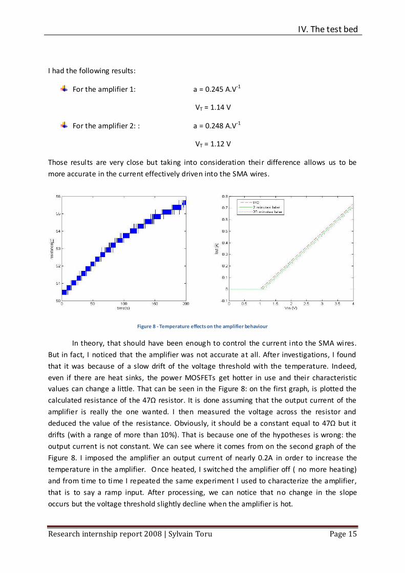
I had the following results:

For the amplifier 1: a = 0.245 A.V-1

VT = 1.14 V

For the amplifier 2: : a = 0.248 A.V-1

VT = 1.12 V

Those results are very close but taking into consideration their difference allows us to be

more accurate in the current effectively driven into the SMA wires.

Figure 8 - Temperature effects on the amplifier behaviour

In theory, that should have been enough to control the current into the SMA wires.

But in fact, I noticed that the amplifier was not accurate at all. After investigations, I found

that it was because of a slow drift of the voltage threshold with the temperature. Indeed,

even if there are heat sinks, the power MOSFETs get hotter in use and their characteristic

values can change a little. That can be seen in the Figure 8: on the first graph, is plotted the

calculated resistance of the 47Ω resistor. It is done assuming that the output current of the

amplifier is really the one wanted. I then measured the voltage across the resistor and

deduced the value of the resistance. Obviously, it should be a constant equal to 47Ω but it

drifts (with a range of more than 10%). That is because one of the hypotheses is wrong: the

output current is not constant. We can see where it comes from on the second graph of the

Figure 8. I imposed the amplifier an output current of nearly 0.2A in order to increase the

temperature in the amplifier. Once heated, I switched the amplifier off ( no more heating)

and from time to time I repeated the same experiment I used to characterize the amplifier,

that is to say a ramp input. After processing, we can notice that no change in the slope

occurs but the voltage threshold slightly decline when the amplifier is hot.

IV. The test bed


Because this phenomenon is very slow, I imagined a control system of the voltage

threshold which would not disturb the rest of the system. Since the emitter current of the

bipolar transistor is very low (for the power MOSFET, VGSmax=-20V, that leads to a maximum

emitter current of nearly and in normal condition VGS is about -2V, which

implies that the emitter current is about 0.2mA), the current across R5 is almost the same as

the one into the SMA wire. Thus, we can use this output as a feedback for our controller. We

are then dealing with very low voltages since R5 is only a 2Ω resistor and as a result, and the

noise is not negligible. To get rid of it, before being processed, the signals are filtered with a

very low-pass filter. I chose a second order filter with a cut-off frequency of 0.25Hz and a

damping ratio of almost 10. Consequently, even if there are sharp changes for the

commanded current, they will not be taken into consideration by the controller. The

controller itself is a simple PI controller with a proportional gain of 500 and an integral gain

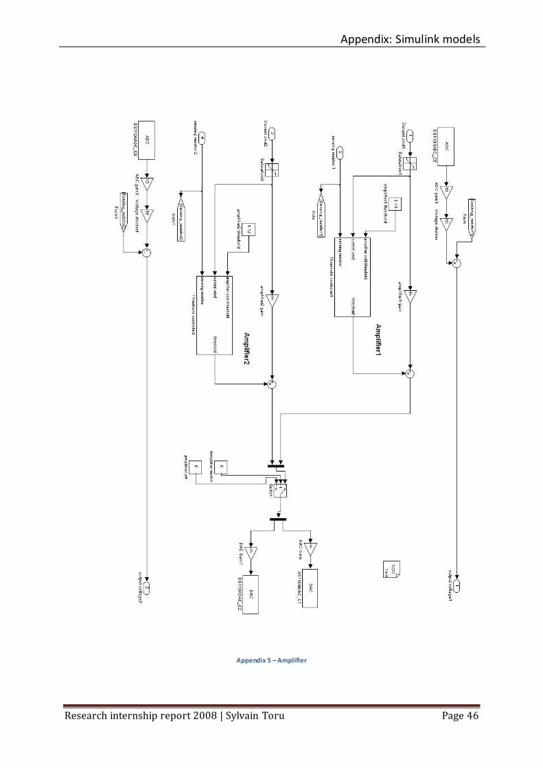
of 10. You can see the block diagrams associated with the power amplifier in the Appendix 5

and Appendix 6.

With this control system, we have now an accurate current source for the SMA wires.

In the Figure 9, we can see this trend of the output to drift with the time (the amplifier is

heating). With different kinds of inputs, the problem remains still the same: although the

output follows the input, it is always with an offset that vary with time. This problem is

solved with the threshold controller, as shown in Figure 10. Indeed, there is no more drift of

the output with the time because it is balanced by the rectification of the voltage threshold.

Now, the average error is zero and the control system has almost not change the behaviour

of the amplifier for every kind of input. The spikes in the graphs are only due to the abrupt

changes in the slope of the input and were already there without any control system.

IV. The test bed


Figure 9 - Response of the amplifier without threshold control

IV. The test bed


Figure 10 - Response of the amplifier with threshold control

IV. The test bed


2. THE LOAD CELLS

Figure 11 - Load cell1

Load cells are used to measure the stress on the SMA wires. Each SMA wire is linked

to a load cell and when there is a stress on it, the strain gauges on the load cell are slightly

deformed and their resistances vary. With a Wheatstone bridge, we can take advantage of

this variation, and once roughly filtered and amplified, we have got an accuracy of 0.3mN

with a 16-bit ADC.

Those load cells are very accurate, but also very fragile. They are rated to 9N, and the

stress on the wires must not rise above 3N, according to the data sheet. When I arrived,

those load cells were new ones because the old ones had been broken by another student.

To take advantage of the accuracy of those cells, they must be calibrated very carefully and

that was part of my work here.

For all the experiments with the load cells, force signals are filtered with a 4 th order

Butterworth filter with a cut-off frequency of 600rad.s -1, and even with this filtering the

signals are still very noisy. For the calibration of the load cells, since we use simple brass

weights, the mass will not change during the experiment. To be accurate on the average

value of the measured force, I used a very low pass filter with a cut-off frequency of 0.25Hz.

To measure the offset and the gain of the load cells, I did two measurements: one without

weight, and one with a weight of 200g. I could then deduce the features of both the load

cells:

Load cell 1: Offset = 0.274 N

Gain = 1.66 V.N-1

Load cell 2: : Offset = 0.203 N

Gain = 1.69 V.N-1

1 Picture from http://www.smdsensors.com/detail_pgs/s215.htm

http://www.smdsensors.com/detail_pgs/s215.htm

IV. The test bed


3. THE LINEAR SLIDE

To move the pulley upward or downward in order to get different stresses on the SMA

wires or to add some motion disturbance to the system, there is a linear slide on which the

pulley is mounted. It is control by a Pittman brushless DC servo motor. The linear slide can

move between two optical switches 20mm far between. There also are two rubber end-

stops in case the motor is not switched off electrically if the slide reaches a switch.

The pulley itself can either be free to rotate or locked, depending on the experiments:

some are done with a pendulum attached to the pulley (position control...) and others need

the pulley to be locked (force control mainly). An optical shaft encoder is linked to the pulley

to measure its angular position. This encoder has a resolution of 8192 bits per revolution,

and the diameter of the pulley is 1.6cm. That leads to an angular resolution of 0.04°.

To control the linear slide, we reset the motor encoder when the bottom of the slide

reaches the lower switch and then we use a PID controller with anti-windup. There is also a

dead zone before the error is being processed because this error is digital since it comes

from an encoder. This prevents the linear slide from oscillating from one encoder count to

another once settled (if the error is not exactly 0 but if it is less than one encoder count, it is

rounded to 0, so this tiny error will not be integrated by the controller). To tune this PID

controller, I chose the Ziegler-Nichols method. Once the encoder reset, the hand is given to

the PID controller. With the derivative and integral gains set to 0, I increased the

proportional gain until the slide became unstable. With this limit proportional gain Kplim and

the period of the oscillations Tu, the Ziegler-Nichols method gives us good parameters for

the PID controller:

Kp = 0.6xKplim

=

Td =

I had the following signal wave with a limit gain of 102.25:

IV. The test bed


Figure 12 - Motor tuning

I could deduce Tu = 19.3ms and Kp = 102, = 104 and Td = 2.4ms. Of course I had to adjust

those gains manually with different kinds of inputs: square waves, sine waves and ramps.

The presence of a saturation bloc k has made the tuning more difficult because the behaviour

of the system becomes non-linear when the saturation block kicks in. The presence of the

anti-windup gain helps but the goal still remains not to get into saturation. Finally, the

different gains I used for this controller are Kp = 102, = 100 and Td = 7ms.

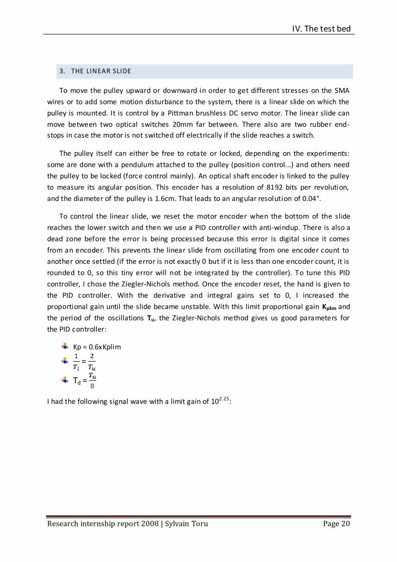
As shown in the Figure 13, the accuracy is pretty good, since the distances are

measured in mm. With a ramp command, except the spikes due to the abrupt changes in the

slope, the accuracy is better than 10µm. With a 2Hz sine wave, the tracking error is still

good, not overrunning 50µm. The response to the square wave is not very satisfying because

of the too big overshoots but it is acceptable for our experiments. Besides, in order not to

damage the wires, I have added a rate limiter between the position command and the

position controller. Thus, the position commanded is, in the worse case, a ramp.

IV. The test bed


Figure 13 - Linear slide response to different kinds of inputs

IV. The test bed


4. SAFETY FEATURES

The load cells and the SMA wires are very fragile and since the linear slide can be very

powerful or the amplifier can drive high currents, several safety features have been

implemented in order to narrow accidents or human errors. Those safety features are

following:

If accidentally, the linear slide was to go further the two optical switches

(programming error), there are two rubber end-stops to prevent the linear slide

from running-off.

A piece of cardboard is placed between the two SMA wires in order to prevent

short-circuits between them.

The strain gauge amplifier which processes the signal from the load cells has an anti-

overload monitor with two levels. When one of the yellow LEDs flashes, it is because

the corresponding wire is overstressed (the force threshold is 9N), and if one of the

red LEDs flashes, it is because the corresponding load cell is broken.

An anti-overload mechanism has been programmed: when one of the two force

signal exceed a certain threshold (5N for our experiments), the amplifier is

immediately switched off and the linear slide moves downward until it reaches the

lower rubber end-stop to remove any residual force into the wires.

A rate limiter has been set to limit the slope of the position command of the linear

slide. Even if the previous anti-overload mechanism cut the power when there is an

overload, it takes a little time, and even if this time is very tiny, if the linear slide is

still moving fast, the stress in the wires can go high above the force threshold. To

prevent that, the rate limiter prevents the linear slide from going faster than a

certain velocity. It has been set to 140mm.s -1.

V. Differential force control of antagonistic SMA actuators


V. DIFFERENTIAL FORC E CONTROL OF AN TAGONISTIC SM A ACTUA TORS

In this section, is mainly described the work of Yee Harn Teh, who worked on designing a fast

and accurate differential force control for a SMA actuator made of an antagonistic pair of

two SMA wires. Note that Figures (...) are all Yee Harn’s work.

1. CONTROL ARCHITEC TUR E

Figure 14 - Overview of the differential force control architecture

To achieve a fast and accurate differential force control in real time, a simple feedback

scheme has to be implemented. For this to be possible, a high-gain PID has been employed

in the differential force controller. In order to improve the velocity and the accuracy, several

mechanisms have been created. They are the anti-slack mechanism, which prevents the

wires from being slack, the rapid-heating mechanism which allows high currents in the wires

in certain limits, and the anti-overload mechanism which prevents the wires from being

over-stressed. Those mechanisms are described in the following sections.

2. THE CONTROLLER

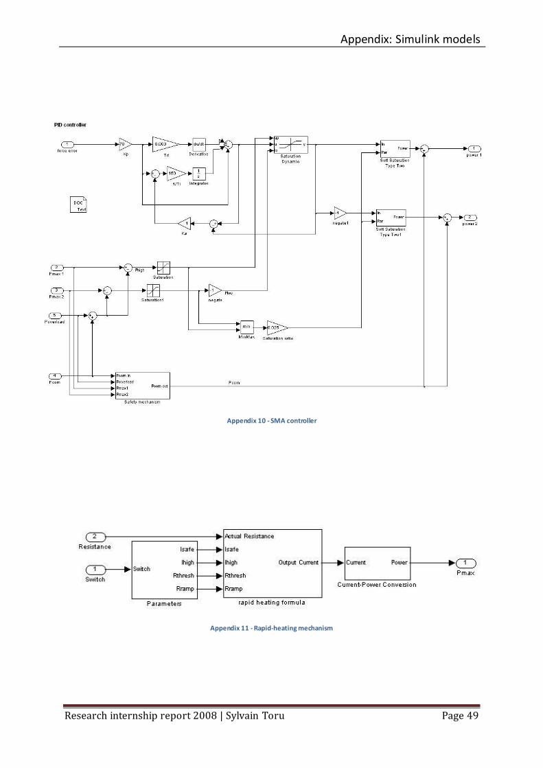
The block diagram of the differential controller is depicted in the Appendix 10. It is a PID

controller with anti-windup. The PID transfer function is given by:



The parameters of the PID controller has been set to Kp = 70, Ti = 6.7ms and Td = 3ms.

They have been chosen with the help of a simulator (a model of the plant has been made by

Yee Harn), and then adjusted on-line. The anti-windup gain is used to reduce the overshoots

due to the saturation block and the integrator: without that, once the output saturated, the

integrator output keep on increasing (or decreasing) and it takes a longer time to leave the

saturation phase.

The saturation block is a dynamic saturation block because the power limits can be

adjusted, mainly by the rapid heating mechanism. To get the best response of both wires,

those limits are calculated separately.

The output of the controller, Pdiff, is a signed power: if it is positive, it is the left wire

which is heated, otherwise, a heating power of –Pdiff is sent to the right wire. Note that

before being sent to the wires, the commanded power goes through a soft saturation block.

Its role is to soften the transition between when the wire is not heated and when it is , by

avoiding discontinuities in slopes. Those blocks have the following equation, based on a

quadratic expression:

where Pout and Pin are the output and input powers of the block and a is an empirical

constant. In the [-4a, 4a] range, this algorithm provide a smooth transition and prevent force

spikes during wire heating activation. The transfer function of the soft-saturation algorithm

is plotted below.

Figure 15 - Soft saturation



3. THE ANTI-SLACK MECHANISM

While cooling, the SMA wires can present the two-ways shape memory effect. That is to

say, the passive SMA can lengthen as it cools, and a few millimetres of slack in the wire can

result. This is a drawback for the control system because before the wire can pull again, it

has to be contracted enough to remove the slack. It implies a loss of time and can also lead

to some mechanical problems such as entanglement or electrical short-circuits.

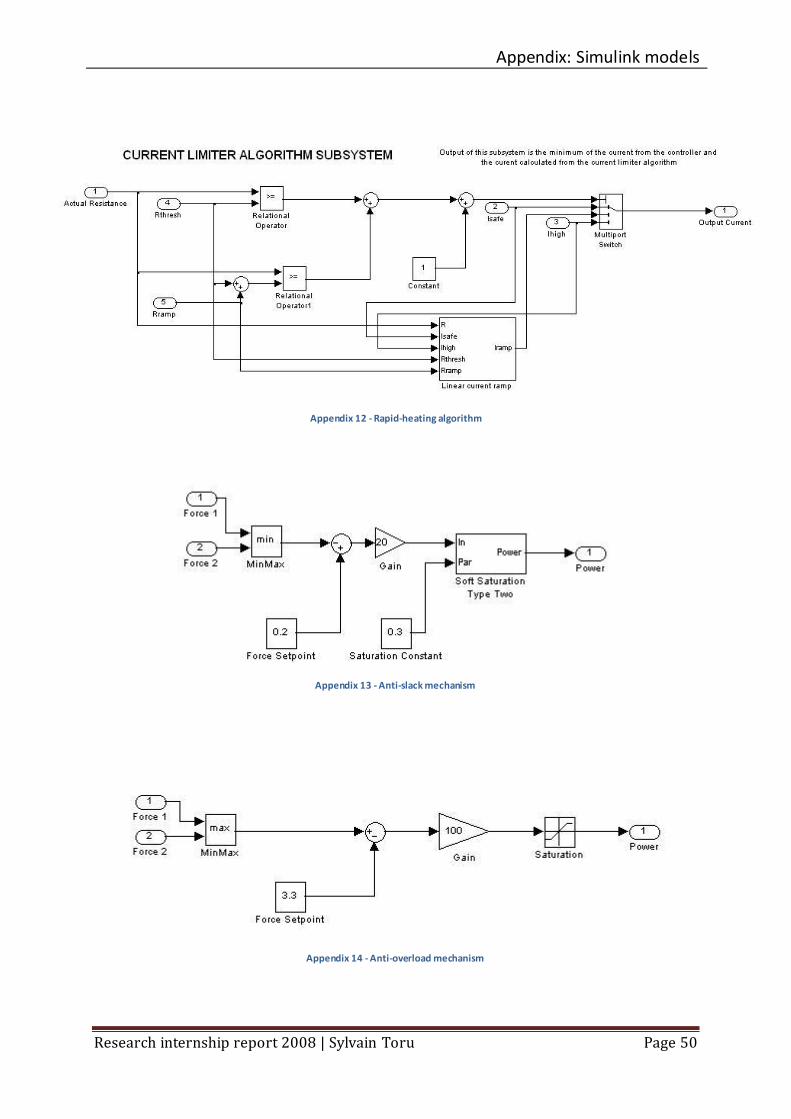
To prevent the wires from becoming slack, we use the anti-slack mechanism, of which

you can see the block diagram in the Appendix 13. It consists in a proportional gain feedback

algorithm that uses the force output. It takes the lower force between the two wires and

compares it to Fmin, the minimum force threshold required in the wires. Then, once

amplified, the signal goes through a soft saturation block of the same kind that the ones

depicted in the previous section, in order to avoid force spikes into the wires when the anti -

slack mechanism kicks in. The resulting power is then added as a common mode to both the

SMA wires in order not to disturb the differential force controller. In the same time, it is

subtracted to the maximum power allowed into the wire not to damage them.

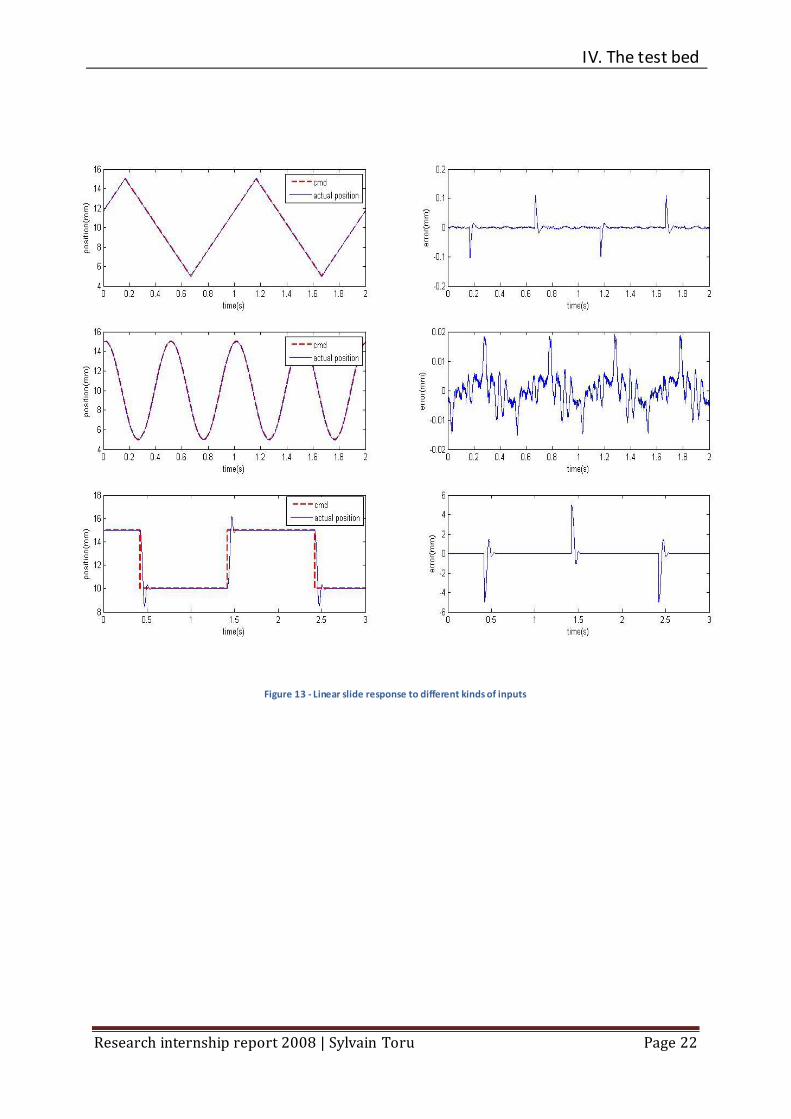
You can see in the following Figure 16 the effectiveness of this mechanism. Without the

anti-slack mechanism, the slack happens around a differential force of 0, when no wire is

pulling on the other. Both wires are cooling and the two-ways shape memory effect can be

observed: the wires lengthened, and there is no longer any control on the differential force,

until the commanded differential force moves away from 0. We can observe errors of more

than 100mN. But with the anti-slack mechanism activated, this problem is fixed since there

still remains a minimum stress in the two wires. The maximum error is then 1mN and it is no

longer due to the slack in the wires but to the abrupt changes in the slope which are quite

well handled by the controller.



Figure 16 - Ramp response without (on the left) and with (on the right) the anti-slack mechanism

4. THE RAPID-HEATING MECHANISM

The speed of an SMA actuator is determined by the rate at which the wire is heated and

by the rate at which they are cooled. According to the wires data sheet, the cooling rate is

lower than the heating one. Using larger currents to heat the wires than the safe current

given in the data sheet make them contract rapidly. However, their use can raise the

temperature into the wires far above the transformation temperature range, and that can

leads to a longer cooling time or worse, to damage the wires.



Figure 17 - Resistance Vs Temperature curve

The rapid-heating mechanism sets upper limits to the maximum power allowed to be

applied in each wire. The idea is to raise those limits in order to improve the actuator

velocity, but only when it is safe to do so. The calculation is done separately for each wire

and is a function of the electrical resistance of each wire. Indeed, the temperature of the

wire and the electrical resistance of the wires are linked. You can see the resistance-versus-

temperature curve in the Figure 17. This curve shows the presence of a hysteresis, which is

due to the hysteresis in the transformations between the austenite and t he martensite

phases. Because of this hysteresis, the temperature in the wire cannot be deduced from the

electrical resistance. However, we can be sure that beyond a certain threshold Rt, the wire is

not overheated. Knowing that, we can increase the maximum power applicable in a wire if

its resistance is above Rt. But when its resistance comes below this threshold, only a safe

power can be applied in the wire. To make the transition between those two ways of setting

the upper limit, the current is ramped between the two limits that is to say that there is a

quadratic transition for the power. The rapid heating formula is implemented as following:

where Isafe = 0.18A is the safe current which cannot damage the wires, according to the data

sheet. Ihigh is the higher current applicable to the wires; R is the actual electrical resistance of

the wire; Rt is the resistance threshold and Rramp is the resistance range on which the ramp

transition is made. For our experiments, we took Ihigh = 0.4A, Rt = 80Ω and Rramp = 4Ω.



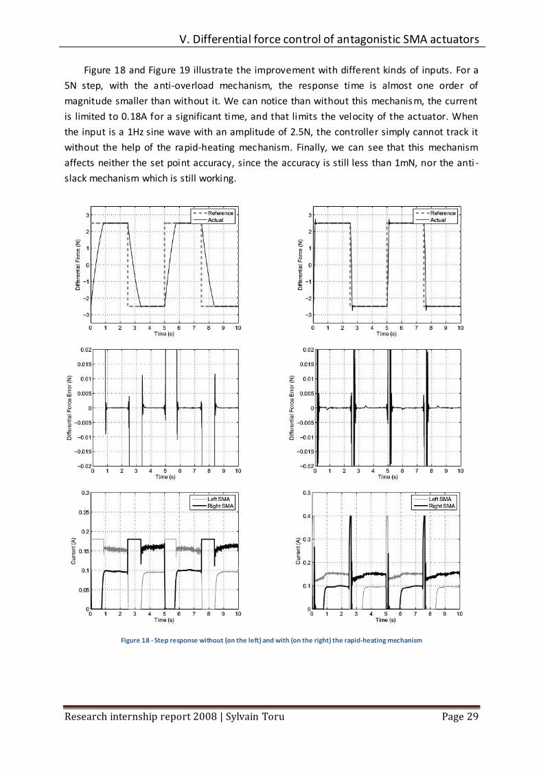
Figure 18 and Figure 19 illustrate the improvement with different kinds of inputs. For a

5N step, with the anti-overload mechanism, the response time is almost one order of

magnitude smaller than without it. We can notice than without this mechanism, the current

is limited to 0.18A for a significant time, and that limits the velocity of the actuator. When

the input is a 1Hz sine wave with an amplitude of 2.5N, the controller simply cannot track it

without the help of the rapid-heating mechanism. Finally, we can see that this mechanism

affects neither the set point accuracy, since the accuracy is still less than 1mN, nor the anti -

slack mechanism which is still working.

Figure 18 - Step response without (on the left) and with (on the right) the rapid-heating mechanism



Figure 19 - Sine response without (on the left) and with (on the right) the rapid-heating mechanism

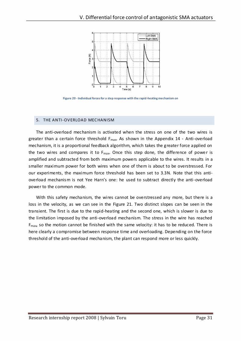
However, we can see in the Figure 20 that there are some big force spikes in the wires.

We wanted the wires to contract in a more rapid way, but that implies that the wires are

pulling strongly and the stress induced can damage them. As a result, we need a mechanism

to prevent the wires from being overstressed.



Figure 20 - Individual forces for a step response with the rapid-heating mechanism on

5. THE ANTI-OVERLOAD MEC HANISM

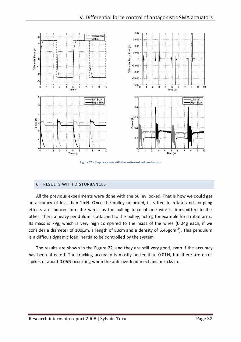
The anti-overload mechanism is activated when the stress on one of the two wires is

greater than a certain force threshold Fmax. As shown in the Appendix 14 - Anti-overload

mechanism, it is a proportional feedback algorithm, which takes the greater force applied on

the two wires and compares it to Fmax. Once this step done, the difference of powe r is

amplified and subtracted from both maximum powers applicable to the wires. It results in a

smaller maximum power for both wires when one of them is about to be overstressed. For

our experiments, the maximum force threshold has been set to 3.3N. Note that this anti-

overload mechanism is not Yee Harn’s one: he used to subtract directly the anti-overload

power to the common mode.

With this safety mechanism, the wires cannot be overstressed any more, but there is a

loss in the velocity, as we can see in the Figure 21. Two distinct slopes can be seen in the

transient. The first is due to the rapid-heating and the second one, which is slower is due to

the limitation imposed by the anti-overload mechanism. The stress in the wire has reached

Fmax, so the motion cannot be finished with the same velocity: it has to be reduced. There is

here clearly a compromise between response time and overloading. Depending on the force

threshold of the anti-overload mechanism, the plant can respond more or less quickly.



Figure 21 - Step response with the anti-overload mechanism

6. RESULTS WITH DISTURBANCES

All the previous experiments were done with the pulley locked. That is how we could get

an accuracy of less than 1mN. Once the pulley unlocked, it is free to rotate and coupling

effects are induced into the wires, as the pulling force of one wire is transmitted to the

other. Then, a heavy pendulum is attached to the pulley, acting for example for a robot arm..

Its mass is 79g, which is very high compa red to the mass of the wires (0.04g each, if we

consider a diameter of 100µm, a length of 80cm and a density of 6.45gcm-3). This pendulum

is a difficult dynamic load inertia to be controlled by the system.

The results are shown in the Figure 22, and they are still very good, even if the accuracy

has been affected. The tracking accuracy is mostly better than 0.01N, but there are error

spikes of about 0.06N occurring when the anti-overload mechanism kicks in.



Figure 22 - Ramp response with the pulley unlocked

VI. Stiffness Control of antagonistic SMA actuators


VI. STIFFNESS C ONTRO L OF ANTAGONISTIC SMA ACTUATO RS

1. OBJECTIVES

The main objective is to make the plant behave like a rotating spring, of which we could

control the stiffness. Controlling the stiffness is very important in robotic applications. If the

stiffness is high, once settled, a robot would not move if you tried to disturb it. However, the

robot would spend a lot of energy trying to keep its position. There is a compromise to make

here and that is why controlling accurately the stiffness is interesting.

2. THE DESIGN

Since we have a fast and accurate differential force controller, we decided to keep it and

add an external position control loop. To implement that loop, we used the optical shaft

encoder present on the pulley. As said previously it has a resolution of 0.04°. Then the

controller is a simple proportional gain, which is in fact the stiffness Kc we want to control.

The input is the position and the output a force, normally very accurately controlled by the

differential force controller. You can see the block diagram of this new system in the

Appendix 1.

3. RESULTS

For all the experiments made with the stiffness controller, the pendulum is attached to

the pulley, which is unlocked.

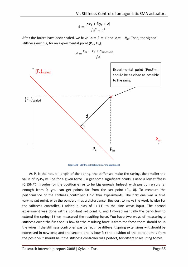
If our plant was a perfect stiffness controller, each point (Pm, Fm), where Pm is the

measured position and Fm the measured resulting differential force, should verify:

where Kc is the commanded stiffness and Pc the commanded position (set point). In a

different way, every point of this kind should be on the ramp drawn in the Figure 23. In this

figure, (Fc)scaled represents the ideal force for a given Pm, divided by Kc to have the same unit

on both axis. Obviously, the experimental points are not exactly on this ramp. To

characterize how far from this ramp they are, that is to say how far from a perfect stiffness

controller the stiffness is, let’s introduce d, the distance from the point to the ramp. d

represents the stiffness error.

We have:

The distance from a point (x1,y1) to a ramp of equation is given by the law:



(Fm)scaled

Pm

d

Pc

Pm

(Fc)scaled Experimental point (Pm,Fm),

should be as close as possible

to the ramp

After the forces have been scaled, we have and . Then, the signed

stiffness error is, for an experimental point (Pm, Fm):

As Pc is the natural length of the spring, the stiffer we make the spring, the smaller the

value of Pc-Pm will be for a given force. To get some significant points, I used a low stiffness

(0.15N/°) in order for the position error to be big enough. Indeed, with position errors far

enough from 0, you can get points far from the set point (Pc, 0). To measure the

performance of the stiffness controller, I did two experiments. The first one was a time

varying set point, with the pendulum as a disturbance. Besides, to make the work harder for

the stiffness controller, I added a bias of +/-11° to the sine wave input. The second

experiment was done with a constant set point Pc and I moved manually the pendulum to

extend the spring. I then measured the resulting force. You have two ways of measuring a

stiffness error: the first one is how far the resulting force is from the force there should be in

the wires if the stiffness controller was perfect, for different spring extensions – it should be

expressed in newtons; and the second one is how far the position of the pendulum is from

the position it should be if the stiffness controller was perfect, for different resulting forces –

Figure 23 - Sttiffness tracking error measurement



it should be expressed in degrees. For both experiments, I measured the stiffness tracking

error in degrees.

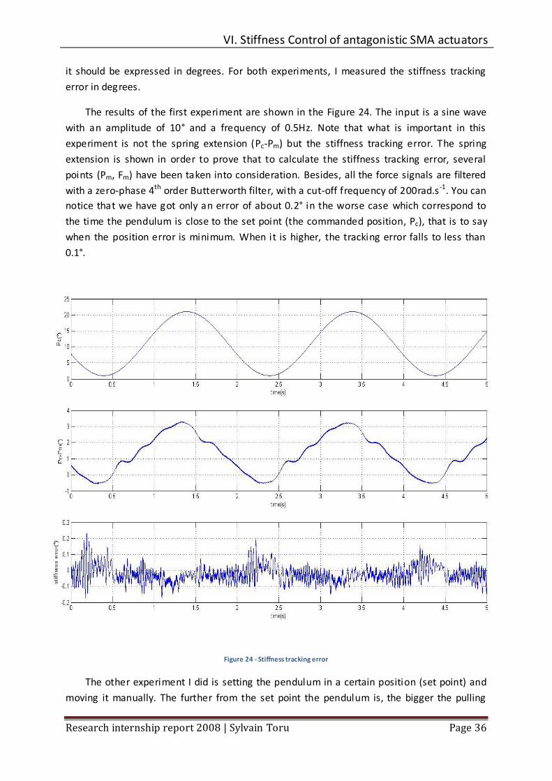
The results of the first experiment are shown in the Figure 24. The input is a sine wave

with an amplitude of 10° and a frequency of 0.5Hz. Note that what is important in this

experiment is not the spring extension (Pc-Pm) but the stiffness tracking error. The spring

extension is shown in order to prove that to calculate the stiffness tracking error, several

points (Pm, Fm) have been taken into consideration. Besides, all the force signals are filtered

with a zero-phase 4th order Butterworth filter, with a cut-off frequency of 200rad.s -1. You can

notice that we have got only an error of about 0.2° in the worse case which correspond to

the time the pendulum is close to the set point (the commanded position, Pc), that is to say

when the position error is minimum. When it is higher, the tracking error falls to less than

0.1°.

Figure 24 - Stiffness tracking error

The other experiment I did is setting the pendulum in a certain position (set point) and

moving it manually. The further from the set point the pendulum is, the bigger the pulling



force developed by the actuator should be. In the following figure (Figure 25), the set point

is 0° and I moved the pendulum from one extreme position to the other (on each side the

steel column block the pendulum at an angle of approximately 24°). In the first graph is

shown the position error ∆P, in degree. The corresponding force should be . The

two last graphs shows how far from this ideal force the measured force is, divided by Kc in

order to make a comparison with the previous stiffness tracking error. Except between 2 and

3s and after 6.5s, the stiffness tracking error is never beyond 0.2°, which reinforce the

previous results.

The two times the measured force do not track the desired force are due to the anti -

overload system. We can see that in the second graph, where clearly either it is the first wire

stress which is saturated to 3.3N or it is the second one. As a result, the current in the wire

cannot be increased because it would lead to a higher stress in the wire and could damage it.

We can also notice that during that saturation, the anti-slack mechanism is no longer doing

its job. If we look at it more carefully, we can see that when the anti-overload kicks in, the

second wire is not slack yet. It becomes slack only when the pendulum pulls higher on the

first wire and to react, the anti-overload mechanism has to subtract more power to both

wires and it has priority on the anti-slack system.

Figure 25 - Stiffness tracking error 2



We have here designed a very accurate stiffness controller. This controller remains

accurate as long as the plant is in its linear domain, that is to say as long as the anti -overload

mechanism does not interfere with it. Depending on the required stiffness Kc, the range in

which we can use the SMA actuator as a spring is limited. For example, with a stiffness of

0.5N/° and a force threshold of 3.3N, the angular range in which the plant behaves like a

spring is +/-6.6°.

VII. Position control of antagonistic SMA actuators


VII. POSITION C ONTRO L OF ANTAGONISTIC SMA ACTUATO RS

1. OBJECTIVES

The goal of that last experiment was to get some good results in position control , with

the pendulum installed, acting for a robot joint for example. Most research investigated in

SMA position control has led to tracking speed of less than 1Hz. Besides, accuracy is never

really good, with error amplitudes greater than 1% of working range.

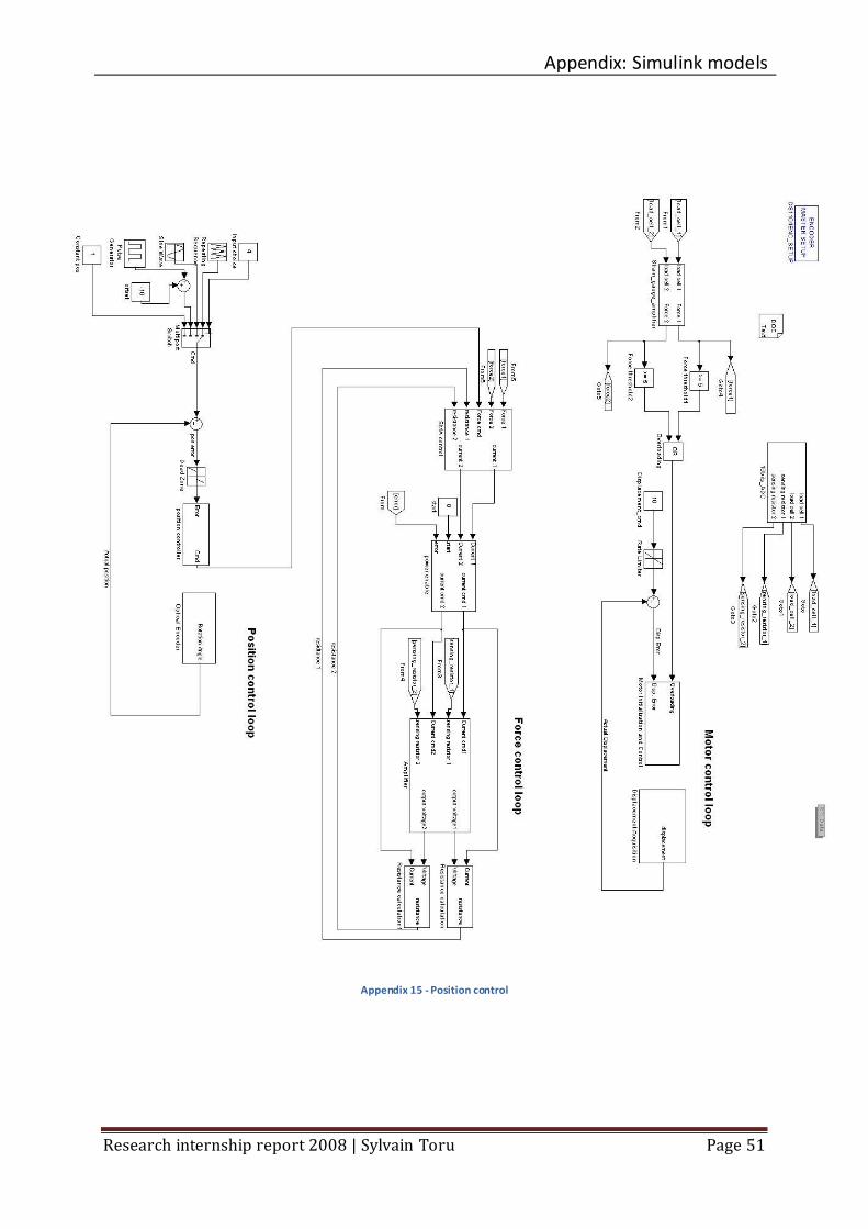
2. THE DESIGN

The rapid-heating, anti-slack and anti-overload mechanisms are kept but the force

controller has change a bit. During his thesis, Yee Harn obtained a model of the plant:

where G(s) is the plant transfer function, and P(s) and F(s) are the Laplace transform of the

heating power and the measured force, respectively. This model is accurate enough at the

high frequency to use it to add a feed-forward term in the controller. With the commanded

force, we can approximately guess what should be the heating power. At the high frequency,

we have:

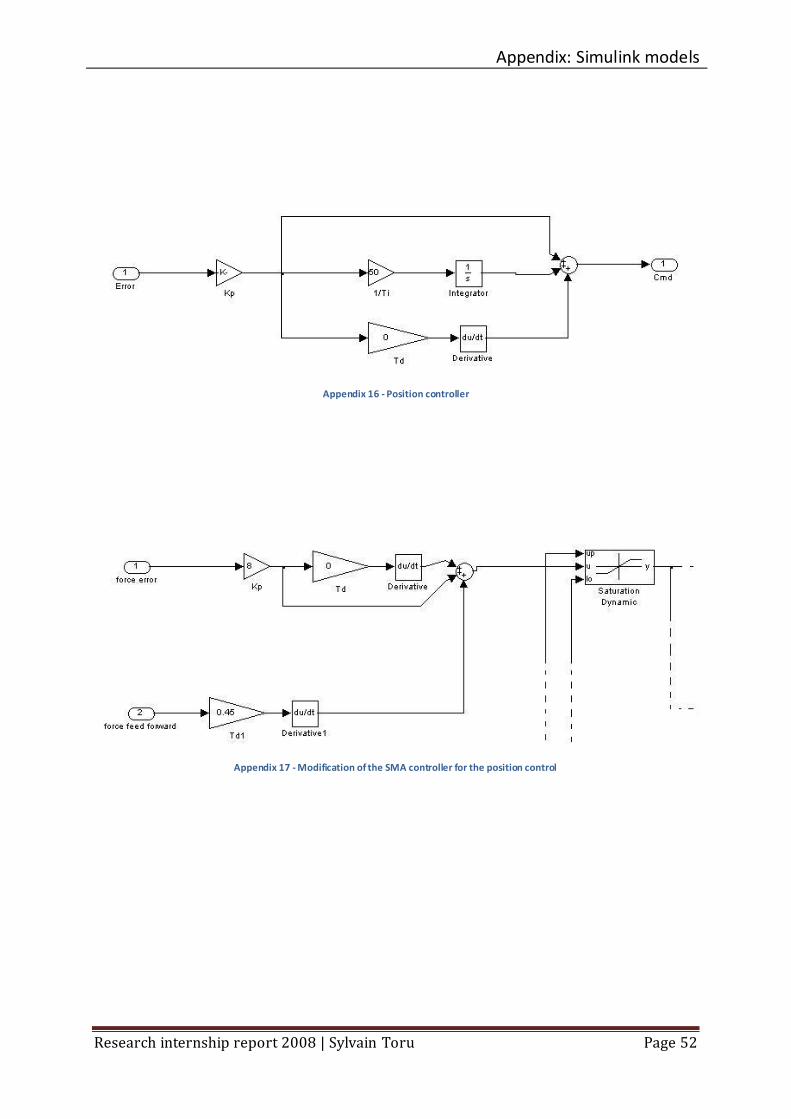
Obviously, we have to be more accurate to control the plant, and we use a PD controller.

That makes the force inner-loop. The position outer-loop is a PID controller. You can see the

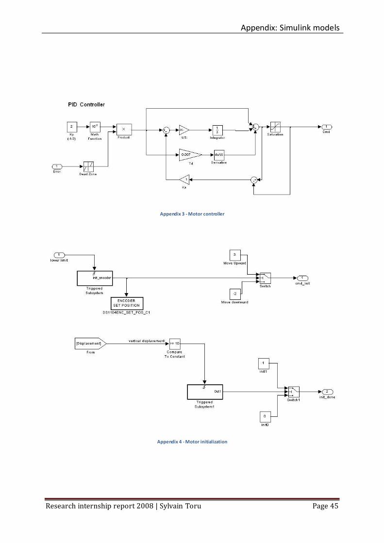
block diagrams in the Appendix 15, Appendix 16, and Appendix 17.

3. RESULTS

With the force and position controller, we have 5 parameters on which we can play to

improve the behaviour of the plant. Manually, it is very difficult to tune those controllers and

I had only little time to get some results. The best ones I got were with the following

settings:

For the position controller: Kp = 0.15

= 50

Td = 0.



Figure 26 - Position ramp response

Figure 27 - 0.5Hz position sine wave response



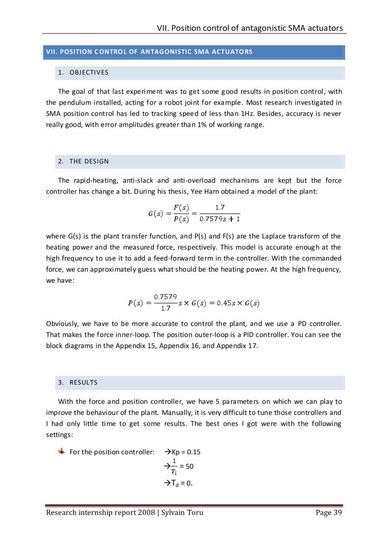
Figure 28 - 1Hz position sine wave response

For the force controller: Kp = 8

Td= 0.

Note that the two differential gains are set to 0. Indeed, they do not improve the

stability of the plant, but it gets it worse. The responses of this position controller are

depicted in the Figure 26, Figure 27, and Figure 28. For the ramp response, we have a n input

with a range of 40° and the error is less than 0.6°. It is a relatively good result but the ramp is

very slow. Indeed, the plant presents limit cycles at not so high frequency. You can clearly

see the difference between the Figure 27 and the Figure 28. The input in both cases is a sine

wave with an amplitude of 20° peak to peak. The only difference remains in the frequency:

the first one is a 0.5Hz sine wave which is slow enough for the actuator to track it, but the

second one is a 1 Hz sine wave, and limits cycles are already present at this frequency.

To conclude this experiment, either some control theory has to be employed to

calculate the best settings for both controllers or a new control system has to be

implemented. Indeed, the limit cycles can be avoided with a best controller because it has

been proven than those kinds of actuators can physically track fastest input.

VIII. Conclusions


VIII. CONCLUSIONS

During this internship, I had the chance to continue a project which is very promising.

Indeed, if well controlled, SMA actuators – which are, remember, only made of two thin

shape memory alloys wires – could have very interesting applications where space is crucial.

Besides, since the test bed was broken when I arrived, I had to fix it and learn about each

part of the experiment so that I understand it in a better way.

The test bed is now operational and the experiments Yee Harn Teh did can be repeated.

Instead of using the precise power amplifier designed for the experiment, we now

use an old one, which is software-controlled and which can be trust to drive the right

current across the SMA wires.

The broken load cells have been replaced by new ones, which have been calibrated.

An experimental protocol has been written to recalibrate them if there is a problem.

The linear slide is controlled by a PID which has been tuned using the Ziegler-Nichols

method, which is documented in the corresponding simulink model and in this

report. It is now fast and accurate.

A new anti-overload mechanism has been implemented.

Once the test bed fixed, I used the differential force controller to transform it in a

stiffness controller. As long as we stay in the linear behaviour of the system, that is to say as

long as the anti-overload mechanism does not kick in, the results are very good. A maximum

error of 0.2° for a random force output has been observed, and this error does not increa se

when the “position error” rises. Of course, the angular range in which the plant behaves like

a spring is not very large because of the maximum stress the SMA can endure. For instance

with a commanded stiffness of 0.5N/° and a force threshold of 3.3N, this range is only +/-

6.6°.

The last try was to build a position controller fast and accurate, with a new control

system, including a force feed-forward term, since a good high-frequency model of the plant

had been made by Yee Harn. The position loop was controlled by a PID. Unfortunately, the

results were not those expected, maybe because of a too short time. The SMA actuators

could only track slow inputs (less than 1Hz) with an accuracy of less than 0.6°. I assume that

with a better tuning of the controllers, the results would have been better. Another thing to

try is to change the whole control mechanism, keeping the rapid-heating, anti-slack and anti-

overload mechanisms which have prove themselves.

To conclude, this 2-month period was very enriching for me, since I did not know

anything about SMAs. I learned many things about them and the world of research, and I

look forward to seeing improvement in their control.

Appendix: Simulink models


APPENDIX: SIMULINK MODELS

Appendix 1 - Stiffness control



Appendix 2 - Motor initialization and control



Appendix 3 - Motor controller

Appendix 4 - Motor initialization



Appendix 5 – Amplifier



Appendix 6 - Threshold controller

Appendix 7 - Power enable

Appendix 8 - Strain gauge amplifier



Appendix 9 - SMA control



Appendix 10 - SMA controller

Appendix 11 - Rapid-heating mechanism



Appendix 12 - Rapid-heating algorithm

Appendix 13 - Anti-slack mechanism

Appendix 14 - Anti-overload mechanism



Appendix 15 - Position control



Appendix 16 - Position controller

Appendix 17 - Modification of the SMA controller for the position control

<Cited works


CITED WORKS

1. Teh, Yee Harn. A control system for achieving rapid controlled motions from shape

memory alloys (SMA) wires. Australian National University. Canberra : s.n., 2003.

2. —. Fast, accurate force and position control od shape memory alloy actuators. Australian

National University. Canberra : -, 2007.

3. Humbeeck, Jan Van. Non-medical applications of shape memory alloys. Materials Science

and Engineering A. 1999, pp. 273-275:134-138.

4. Kohl, M. Shape memory microactuators. s.l. : Springer, 2007.

Fast and accurate position control of shape memory alloy...

Documents

Transcript of Fast and accurate position control of shape memory alloy...