Formulation and Calibration of Fast, AccurateVehicle Motion Models

Neal Seegmiller

Abstract High performance wheeled mobile robots (WMRs) require fast, accuratemotion models for planning and control. This thesis addresses two challenges to pro-ducing these models: the tradeoff between fidelity and speed in model formulation,and the need for laborious calibration procedures. To address the first challenge, Ipropose the formulation of “enhanced” 3D velocity kinematic models that providecomparable accuracy to comprehensive physics-based models, but at a fraction ofthe computational cost. In a modular way for any WMR design, the motion pre-diction problem is formulated as the solution of a differential-algebraic equation(DAE), with wheel velocity constraints derived using a vector algebra-based ap-proach. These models account for articulations on uneven terrain, and are enhancedto account for slip, powertrain dynamics, and extreme conditions such as rollover.To address the second challenge, I propose the convenient self-calibration of thesemodels using an online integrated equation error (IEE) approach. The IEE approachalso enables the characterization of non-systematic error, such that the planner mayreason about the uncertainty of motion predictions. I will prove experimentally thatmodels formulated and calibrated as proposed are both faster and more accuratethan alternatives. This thesis unifies and extends successful prior work by AlonzoKelly, Forrest Rogers-Marcovitz, and myself.

1 Problem Description

Fast, accurate motion models are essential for planning and control on high per-formance wheeled mobile robots (WMRs). Motion models enable the predictionof future state, given an initial state and control inputs as a function of time. ForWMRs, state typically means pose (position and orientation) of the vehicle bodyframe. State may also include joint positions such as steer angles if applicable.

Neal Seegmiller is a Ph.D. candidate at the Robotics Institute, Carnegie Mellon University, e-mail:nseegmiller@cmu.edu

1

2 Neal Seegmiller

WMR planners require predictively accurate motion models to plan feasiblepaths, and controllers require accurate models to execute them. In some situations,approximately following the planned path may be sufficient. Closed-loop controllerscan accomplish this given just an approximate motion model and frequent positionfeedback (e.g. via GPS, INS, visual odometry). Examples include WMR controllersthat do not predict slip, but instead detect and compensate for it [14], or robustly re-cover from it [29]. However, reliance on feedback control has disadvantages. Feed-back control does not prevent error, but only attempts to correct error after it occurs.Most WMRs can’t move laterally so a smooth return to the target path without back-tracking may be impossible if obstructed. Given a poor motion model, the WMRplanner/controller may attempt dangerous maneuvers, such as sharp turns that causerollover.

While not always required, precise trajectory prediction is necessary in chal-lenging situations. Consider a self-driving car maneuvering in highway traffic, ora planetary rover driving on the edge of a cliff or on steep sandy slopes. Considerwhen an obstacle can’t be circumvented but must be traversed, such as large debrisspanning a passageway in a disaster site.

Motion model speed is equally important. In receding horizon model predictiveplanning (MPP), which has been implemented successfully on the high performancerobots Crusher and Boss [16], the model’s computational cost limits both the timehorizon and the number of paths that can be evaluated during replanning. Thesedirectly affect the ability of the planner to find collision-free paths when travelingat high speeds. Other predictive WMR planning schemes are possible (e.g. RRT[28], lattice [37]), but all benefit from an efficient model. While lattice (and other)planners precompute a “control set” of feasible trajectories, variations in terrainshape and terramechanical properties necessitate local changes to the control set[15]. Given a slow model making these changes would be prohibitively slow.

Note that motion models useful for planning/control may also have application toposition estimation, such as dead-reckoning in GPS-denied environments; howeverthe computational speed requirement is relaxed when estimating only the currentlocation.

Sections 1.1 and 1.2 describe two fundamental challenges to producing WMRmotion models.

1.1 Challenge 1: Fidelity vs. Speed Tradeoff

All motion models can be placed on a spectrum of complexity, with high fidelityphysics-based models at one end and simple 2D Dubins car-like models at the other.Unfortunately, higher fidelity typically means slower computation.

Formulation and Calibration of Fast, Accurate Vehicle Motion Models 3

1.1.1 Related Work on WMR Model Formulation

In this document, the descriptor “comprehensive physics-based” is used to refer tomodels that predict the motion of each individual body in the system using a second-order differential equation with force/torque inputs. For a WMR, bodies capable ofrelative motion include the frame, axles, wheels, etc. Each body must have a knownmass and rotational inertia. Motion prediction involves solving for accelerations anddouble integrating to obtain pose.

Examples of physics-based vehicle simulators include the commercial softwarepackages Adams/Car and CarSim. To improve computational efficiency CarSimuses kinematics and compliance (K&C) lookup tables instead of simulating sus-pension bodies but still runs only ten times real-time on a 3 GHz PC [33], not fastenough for model predictive planning.

Another example is Rover Analysis, Modeling, and Simulation (ROAMS) de-veloped by NASA JPL for the Mars Exploration Rovers. ROAMS modeled the fullkinematics and dynamics of the rovers as well as wheel/soil slippage/sinkage inter-action [21]. Simulations ran no faster than real-time, however, and so ROAMS wasprimarily used for Monte Carlo Simulation to evaluate rover designs, not for motionplanning.

A few have attempted motion planning with physics-based models. For example,the planning algorithm proposed by Ishigami et al. performs complete dynamic sim-ulation of each candidate path; but slow simulations make the algorithm unsuitablefor real-time operation. In their own experiment, evaluating just 4 paths (that wouldeach take the robot approximately 3 minutes to execute) took 47 minutes [20]. Moreoften, in research and in practice, model predictive planning is implemented usingsimple 2D Dubins car-like motion models with curvature limits [13] [26].

Limited prior work exists on WMR planning/control with models that compro-mise between fidelity and speed. Iagnemma provided a model-based approach tocomputing costs in an A* planning framework for planetary rovers. Costs are com-puted based on both 3D kinematic analysis and force analysis, which considerslimits on tractive force. Iagnemma’s terramechanics-based model of wheel/terraininteraction contains some approximations to reduce computation. [18]. Yu et al. de-veloped a model of skid-steered vehicles that accounts for motor limits and variableshear stress on the tires, intended for use in sampling-based model predictive con-trol. Howard investigated motion planning on uneven terrain with motion modelsthat include suspension articulations, latencies, limits, etc. [15]. Howard acknowl-edges the tradeoff between fidelity and speed but resolving it was not within thescope of his thesis.

While several have investigated planning with realistic motion models, few havepublished general methods to deriving such models for arbitrary vehicle configu-rations. Muir and Neuman published one of the earliest general approaches to 2Dkinematic modeling of WMRs. They first derive a graph of homogenous transformsrelating wheel and robot positions, then differentiate with respect to time to ob-tain the velocity kinematics [34]. More recently, Tarokh and McDermott provideda similar transform-based approach to deriving full 3D kinematic models [43]. In

4 Neal Seegmiller

addition, they show how predicting motion that satisfies constraints can be treatedas a nonlinear optimization problem. Others have derived and simulated 3D WMRkinematics with specific objectives, such as mechanisms that enable rolling with-out slipping [7][6] or precise localization [27], but provide no general method forderiving WMR models.

1.1.2 What is Desired? WMR Model Formulation

An approach is desired to generate WMR motion models that meet both fidelity andspeed requirements. With respect to fidelity, the models should accurately :

• account for 3D articulation of the chassis/suspension when driving on uneventerrain (in a modular way that accommodates any joint configuration)

• account for wheel slip• account for powertrain dynamics, including limits and latencies• predict the onset of extreme conditions such as rollover and loss of traction

I propose that enhanced velocity kinematic models can meet these requirements.The last three items above are the enhanced capabilities, not typically provided bykinematic models. Of course kinematic models can never predict motion during ex-treme conditions like physics-based models can, but this limitation can be mitigatedby predicting the onset of these conditions so as to prevent them.

With respect to speed the models should:

• be capable of simulation 100 to 1000 times faster than real-time

1.2 Challenge 2: Difficulty of Calibration

Besides computational inefficiency, high fidelity models have another disadvantage:they require the identification of numerous parameters, and realistic model com-plexity does not ensure accuracy unless these parameters are identified properly.

High fidelity terramechanics-based models of wheel/soil interaction require pa-rameters such as soil cohesion, internal friction angle, shear deformation modulus,sinkage ratio, etc. [19]. Accurate force-based powertrain models require parameterssuch as motor saturation and power limits [45], or engine torque/speed character-istics, rotational inertia, etc. (in CarSim). Even simple 2D kinematic models havedimensional parameters such as wheel radii, track width, etc.

1.2.1 Related Work on WMR Model Calibration

There are several approaches to identifying WMR model parameters.One may analyze subsystems in isolation. For example, Ding et al. determined

planetary soil parameters by driving a single wheel in an instrumented testbed [9].

Formulation and Calibration of Fast, Accurate Vehicle Motion Models 5

Commercially available actuator test rigs equipped with force/torque sensors mightbe used to model individual drive motors. However, this is time consuming andthe vehicle-level motion model may not match experimental data even if subsystemmodels do.

Alternatively, parameters may be identified by observing deviations as the ve-hicle executes preprogrammed trajectories. For example, Borenstein and Feng pro-posed an early odometry calibration procedure called the “UMBmark” test, in whichwheelbase and wheel diameter are identified by traversing a square path [4]. Iag-nemma proposed an online terrain parameter calibration procedure which requires avery simple preprogrammed maneuver. While driving on flat terrain and measuringmotor torque and chassis configuration, one wheel is temporarily driven faster thanthe others [18].

Self-calibration of motion models during normal operation is the ideal approach;it is convenient and it makes possible adaptation to changing conditions such asterrain transitions or a flat tire. Toward this end, Kelly [22], Antonelli et al. [2], andMartinelli et al. [31] have proposed methods to calibrate odometry to trajectories ofvaried shape. Importantly, by exploiting equations for the propagation of odometryerror, these methods allow for significant time-separation between observations ofrelative pose.

The best-fit estimates of motion model parameters minimize the error in futurepose predictions; however, some remaining non-systematic error is unavoidable dueto limited model fidelity, limited perception (e.g. of terrain shape), or truly unpre-dictable disturbances (e.g. wind gusts). [22] and [31] not only remove systematicerror by calibrating odometry parameters, but also characterize the remaining non-systematic error.

1.2.2 What is Desired? WMR Model Calibration

The papers on odometry self-calibration cited above only apply to simple 2D veloc-ity kinematic motion models. We desire a calibration process for more sophisticatedmodel formulations that satisfy the fidelity requirements listed in Section 1.1.2. Thedesired calibration process should:

• not require the execution of preprogrammed trajectories, but run online duringnormal operation

• require only intermittent observations of relative vehicle pose• be computationally tractable• learn a model of non-systematic error• adapt quickly to changing terrain and hardware conditions without overfitting

Susceptibility to overfitting depends on both the model formulation (e.g. the param-eterization of wheel slip) and the time-variance of parameter estimates allowed bythe calibration process.

6 Neal Seegmiller

1.3 Hypothesis Statement

I hypothesize that enhanced 3D velocity kinematic motion models can be formulatedfor WMRs that are, compared to comprehensive physics-based models, equivalentlyaccurate (under normal conditions) but computationally cheaper by at least an orderof magnitude. These models will satisfy all itemized requirements in Section 1.1.2,which are not met by any existing model formulation in the literature.

Furthermore, I hypothesize that all necessary parameters of these models canbe conveniently self-calibrated. The calibration process will satisfy all itemized re-quirements in Section 1.2.2, which are not met by any existing process in the litera-ture.

2 Student Progress To Date

I have made progress addressing both the tradeoff between fidelity and speed and thedifficulty of calibration, but until now in unconnected projects. Sections 2.1 and 2.2describe my prior contributions to formulating WMR motion models and vehiclemodel identification respectively. Section 2.3 presents a survey of related work thatmay be leveraged to address limitations of the current formulation.

2.1 Formulation of WMR Motion Models

My advisor, Alonzo Kelly, has for some time been developing a vector algebraformulation of WMR velocity kinematics [24], and a corresponding differential-algebraic equation (DAE) formulation of velocity kinematic motion prediction. Irecently validated this approach in a full 3D test [25]. A brief summary is presentedhere.

2.1.1 Theory

The vector algebra formulation of velocity kinematics is based on a theorem inphysics commonly known as the Coriolis Equation or Transport Theorem; it con-cerns the dependence of measurements on the motion of the observer.

Let the letter f denote a frame of reference associated with a fixed observer andm with a moving observer. Due to their relative angular velocity (⇀ω

fm) the observers

would measure different time derivatives of the same vector ⇀v, related as follows:

d⇀vdt

∣∣∣∣f

=d⇀vdt

∣∣∣∣m

+⇀ω

fm×

⇀v (1)

Formulation and Calibration of Fast, Accurate Vehicle Motion Models 7

⇀v in (1) may represent position or one of its derivatives (linear velocity, acceleration,etc.).

Using the Transport Theorem, we can derive the transformation of linear velocitybetween frames undergoing arbitrary relative motion. The velocity of an object o inframe f is computed from the apparent position and velocity of the object in framem and the relative velocity between frames as follows:

⇀vfo =

⇀vmo +

⇀vfm +

⇀ω

fm×

⇀rmo (2)

Here ⇀r denotes position and ⇀v denotes linear velocity. The notation ⇀ba means the

vector quantity is of frame a with respect to frame b.Using (2) one can derive “wheel equations” that relate velocity at the wheel/terrain

contact points to velocity of the WMR body frame. To demonstrate, consider this2D example of a WMR with four steerable wheels, each offset from its steeringaxis. Figure 1 depicts the (w)orld, (v)ehicle, (s)teering, and (c)ontact frames and therelative position vectors between them. Note that there are four s and c frames, onefor each wheel. The corresponding wheel equation is:

⇀vwc =

⇀vwv +

⇀ω

wv ×

⇀rvs +

⇀ω

wv ×

⇀rsc +

⇀ω

vs ×

⇀rsc (3)

(a) (b)

Fig. 1 A 2D diagram of a wheeled mobile robot with four steerable wheels, each offset from itssteering axis. (a) Depicts steer angles and dimensions. (b) Depicts the four frames referenced inthe wheel equation, as well as relative position vectors between them.

Notice that, for simplicity, we do not include wheel rotation in (3); instead weequivalently consider that a fixed wheel slides with respect to the terrain. In the caseof rolling without slipping, the magnitude of ⇀v

wc is proportional to the product of

wheel radius and angular velocity, and the direction is along the forward axis of thec frame.

8 Neal Seegmiller

Using the wheel equations we may solve for either the forward or inverse velocitykinematics. Let the term inverse kinematics refer to the problem, relevant to control,of computing the wheel velocities from the body velocity. This can be done usingthe wheel equations directly. Let the term forward kinematics refer to the problem,relevant to estimation, of computing the body velocity from wheel velocities. Tocompute body velocity in our example we rearrange (3) as follows:

[I [⇀r

vc]T×

] ⇀vwv

⇀ω

wv

=⇀v

wc −

⇀ω

vs ×

⇀rsc (4)

The notation []× denotes a skew-symmetric matrix (formed from the vector insidethe brackets) used represent a cross product as a matrix multiplication. Specifically,we made the following substitution: ⇀

ω×⇀r = −

⇀r × ⇀ω = −[⇀r ]×

⇀ω = [⇀r ]T

×

⇀ω. We stack

these equations for all wheels into a single matrix equation of the form:I [⇀r

vc1]T×

......

I [⇀rvc4]T×

⇀vw

v⇀ω

wv

=

⇀v

wc1−

⇀ω

vs1×

⇀rs1c1

...⇀v

wc4−

⇀ω

vs4×

⇀rs4c4

(5)

then solve for the vehicle velocity using the pseudoinverse.This vector algebra-based method of propagating velocities through a kinematic

chain is a classical one previously applied to robotic manipulators [30]. For WMRs,one primary advantage of this approach compared to transform-based approaches(i.e. Muir and Neuman [34], Tarokh and McDermott [43]) is that differentiation oftransform chains is not required to compute wheel Jacobians, which can be tediousto do analytically or expensive numerically.

In [25], I validated this approach for the derivation of full 3D WMR velocitykinematics. The 3D motion prediction problem is then best formulated as the solu-tion of a semi-explicit differential-algebraic equation (DAE):

x = f (x,u)

c(x) = 0 (6)D(x)x = 0

Here the state x includes the pose of the body frame and joint positions (angles forrotary joints, lengths for prismatic joints). Inputs u include wheel angular velocitiesand driven articulation rates (which correspond directly to elements of x), or vari-ables from which these may be calculated according to f (x,u). The inputs do notspecify the time-derivative of all state variables; computing a complete solution forx requires constraints.

Constraints of the form D(x)x = 0 are non-holonomic; they include restrictionsthat wheels not slip with respect to the terrain. Each row of the D matrix is a dis-allowed direction in state space. Constraints of the form c(x) = 0 are holonomic;they include restrictions that wheels not penetrate the terrain surface. Holonomic

Formulation and Calibration of Fast, Accurate Vehicle Motion Models 9

constraints can be enforced to first-order by requiring that cx x = 0, where cx is theJacobian of c(x) with respect to x (see Yun and Sarkar [46]). For terrain-followingconstraints, this equates to disallowing velocity at the wheel/terrain contact pointin the direction of the terrain-normal; in practice, this can be done without explicitcomputation of the Jacobian cx.

Note that one 3D wheel equation provides two (non-holonomic) wheel slip con-straints and one (holonomic) terrain-following constraint. Depending on vehicle de-sign, there may be additional constraints between joint positions.

Lagrange multipliers are used to find a solution for x that satisfies all constraints:[I CT

C 0

] [xλ

]=

[f (x,u)

0

](7)

C =

[cx

D(x)

]Baumgarte’s stabilization method may be used to prevent drift in the enforcementof holonomic constraints [46].

This one-step method of solving a DAE to predict motion is more elegant and ac-curate than the alternative proposed by Tarokh and McDermott. For each time step,they first compute the new (x,y) location and heading by unconstrained integration,then perform iterative nonlinear optimization to solve for free state variables (e.g.suspension angles) [43]. Because our DAE approach produces constrained deriva-tives, we can use higher-order integration methods such as Runge-Kutta which areaccurate even for large step sizes.

2.1.2 Experimental Results

I validated this approach to deriving and simulating 3D velocity kinematics on theZoe rover. Zoe has four independently driven wheels on two passively articulatedaxles. The axles are free to rotate about their steering and roll axes; but a mechanismforces symmetry in the front and rear axle roll angles (see Figure 2).

Fig. 2 Zoe’s axles are free to passively rotate about their steering and roll axes, but the roll anglesare constrained to be symmetric.

In a physical experiment, Zoe was commanded to drive straight while its leftwheels traversed a ramp-shaped obstacle. Body orientation, articulation angles, and

10 Neal Seegmiller

wheel velocities were logged as a function of time. The experiment was then recre-ated in both a physics-based simulation (using Open Dynamics Engine) and a 3Dvelocity kinematic simulation (using the approach presented here). As seen in Fig-ure 4, both simulations closely match the experimental results, but the kinematicsimulation is computationally much simpler. For additional details refer to [25].

Fig. 3 Photographs and screenshots of the Zoe rover captured during (from left to right) a physicalexperiment, physics-based simulation, and kinematic simulation.

0 10 20 30 40 50

−8

−6

−4

−2

0

2

4

6

8

time (s)

de

g

Physical Experiment

θ f

θ r

φ f

φ r

yaw

0 10 20 30 40 50

−8

−6

−4

−2

0

2

4

6

8

time (s)

de

g

Dynamics Simulation

θ f

θ r

φ f

φ r

yaw

0 10 20 30 40 50

−8

−6

−4

−2

0

2

4

6

8

time (s)

de

g

Kinematic Simulation

θ f

θ r

φ f

φ r

yaw

Fig. 4 Plots of steering (θ), suspension (φ), and vehicle yaw angles vs. time recorded during (fromleft to right) a physical experiment, physics-based simulation, and kinematic simulation using theproposed vector algebra-based model. Both simulations correctly predict a terminal heading errorof approximately 2.5◦

2.1.3 Limitations

There are important limitations to our current formulation of velocity kinematicmotion models. We have not yet rigorously specified how to formulate the motionprediction problem as a DAE in a modular way, for any WMR joint configuration.Furthermore, we have not specified how to optimize solution of the DAE for effi-ciency, or how to best handle overconstraint.

Formulation and Calibration of Fast, Accurate Vehicle Motion Models 11

Most importantly, to date we have only enforced no-slip constraints at the wheelsbut we wish to enforce realistic, experimentally-calibrated slip models. Further-more, current models do not account for powertrain dynamics, or predict the onsetof extreme conditions such as rollover and loss of traction.

Finally, quantitative comparison of computational speed with alternative mod-els has not been possible yet, because the proposed model has only been imple-mented in MATLAB and is not yet optimized for speed. Furthermore, we have nodirectly analogous physics-based model to compare with. Existing software mightrun slower than ours because of capabilities we do not require; for example, OpenDynamics Engine’s geometry-based collision detection might be more expensivethan our discretized approach.

2.2 Vehicle Model Identification

For over two years I have worked in collaboration with Alonzo Kelly and ForrestRogers-Marcovitz on an integrated equation error (IEE) approach to vehicle modelidentification. I have successfully used this approach to calibrate model parametersrelating to slip [40], as well as odometry and powertrain dynamics [39]. A brief sum-mary is presented here; but for a complete discussion of IEE theory, online/offlineimplementations, and experimental results see [41]

2.2.1 General IEE Theory

System models are commonly expressed in the form of a differential equation:

x = f (x,u, p) (8)

where x is the state vector, u is the input vector, and p is the vector of parameters tobe calibrated. The classical model identification approach is to use the differentialequation directly, which requires observations of x and x. Often x is not measureddirectly, so measurements of x are numerically differentiated with respect to time.For example, in the Springer Handbook of Robotics manipulator inertial parametersare estimated this way, which requires double differentiation of joint angle data [42].

In contrast, using the IEE approach we calibrate the parameters p to the inte-grated dynamics:

x(t) = x(t0) +

∫ t

t0f (x(τ),u(τ), p) dτ (9)

In effect, we integrate the prediction rather than differentiate the measurement,which has several advantages.

First, numerical time-differentiation of measurements can be noisy, and requiresaccurate timestamps and high-frequency sensors. Low-frequency measurements aresufficient for IEE, which reduces the amount of ground truth information needed.

12 Neal Seegmiller

For example, odometry could be calibrated by driving various paths between a fewcarefully surveyed points instead of requiring continuous position feedback.

In addition, integrated predictions may compound the effects of errors causedby poor parameter estimates until they become observable and/or easier to disam-biguate. On WMRs for example, angular velocity error (e.g. caused by a poor trackwidth estimate) has no instantaneous effect on linear velocity, but it produces ob-servable position error after traveling some distance. A gyro can see the effect di-rectly (if available) but even GPS can see it when IEE is used.

Finally, IEE allows us to optimize prediction accuracy for the exact time hori-zon (t− t0) that the planner cares about. In practice, this is especially important inthe calibration of stochastic models. Even if assumptions of the stochastic models(such as white noise) are violated, using IEE these models can still be calibrated toproduce accurate uncertainty estimates.

Calibrating to the system integral (9) also presents challenges. The linearizationprocess must linearize an integral instead of simply the function f (). Uncertainty inthe measurement of initial state x(t0) must be accounted for, as well as correlationbetween the measurements of x(t0) and x(t).

To update parameter estimates using the IEE approach we require a prediction,a measurement, and the Jacobian of the prediction with respect to the parameters.If using an extended Kalman filter (EKF) we also require the measurement uncer-tainty; but for brevity this is not presented here.

Assume measurements of state x are obtained at times t0 and t. Given the initialmeasurement of state x(t0), time-indexed values of the inputs u during the interval(t0,t), and our current estimates of the parameters p, we predict the state at the futuretime t according to (9). We withhold any state measurements obtained during the in-terval. We attribute the difference between this prediction (denoted by h(p)) and themeasurement of x(t) to inaccurate parameter estimates, and update p accordingly.Computing the change in parameter values requires the Jacobian H = ∂h(p)/∂p.

The Jacobian H can always be computed numerically, but in some cases it canbe computed more efficiently by linearizing the system integral. By differentiating(8), we obtain the linearized perturbative dynamics for deterministic (also known assystematic) error:

δx(t) = F(t)δx(t) +G(t)δu(t) (10)

where F and G are Jacobian matrices:

F =∂ f

∂x, G =

∂ f

∂u(11)

The solution to the first-order differential equation (10) is as follows. We will callit the vector convolution integral:

δx(t) =Φ(t, t0)δx(t0) +

∫ t

t0Γ(t, τ)δu(τ)dτ (12)

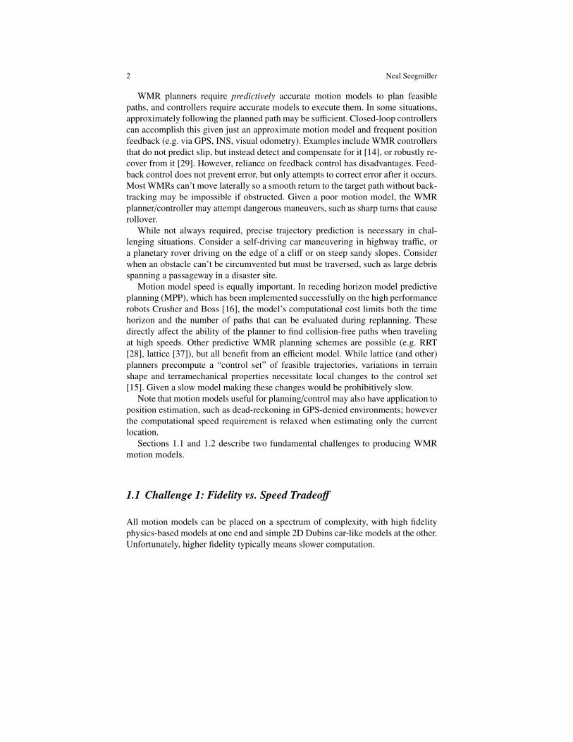
Formulation and Calibration of Fast, Accurate Vehicle Motion Models 13

The key to this solution is derivation of the transition matrixΦ(t, τ), which is omittedhere for brevity. We also define the input transition matrix Γ(t, τ) = Φ(t, τ)G(τ) forconvenience. In short, (12) attributes errors in the prediction of terminal state δx(t)entirely to errors (or perturbations) in the inputs δu, which in turn we attribute toerrors in our parameter estimates.

To do so, we must formulate the system differential equation (8) such that theparameters are confined to modulating the inputs:

x = f (x,u(p)) (13)

Note that this is still the general case. If the system model is of the form x =

f (x,u(p), p), for every parameter pi that is not confined to modulating the inputs,simply create a new input u = pi that depends trivially on the parameter.

Based on (12) and (13) the Jacobian is:

H ≈∫ t

t0Γ(t, τ)

∂u(p, τ)

∂pdτ (14)

Notice that we use the Leibniz rule to move the partial derivative inside the integral.Because (14) is based on linearized error dynamics, it is only a valid approximationof ∂h(p)/∂p for small perturbations of the parameters.

Of course, even after calibrating the parameters p, predictions of x(t) will notbe perfect; some non-systematic error will remain. To characterize this remainingerror, we calibrate a model of uncertainty propagation which proceeds directly fromthe linearized dynamics for systematic error above. By squaring and taking the ex-pectation of (10) we obtain the stochastic error dynamics:

.P(t) = F(t)P(t) + P(t)F(t)T +G(t)Q(t)G(t)T (15)

where:

P(t) = cov(δx(t)

)= E

[δx(t)δx(t)T ]

(16)

Q(t) = cov(δu(t)

)= E

[δu(t)δu(t)T ]

(17)

The solution to the stochastic differential equation (15) is as follows. We will callit the matrix convolution integral:

P(t) =Φ(t, t0)P(t0)Φ(t, t0)T +

∫ t

t0Γ(t, τ)Q(τ)Γ(t, τ)T dτ (18)

Q(τ) is the covariance of random input noise at time τ (assumed to be white giventhat systematic perturbations are removed), and P(t) is the resulting covariance interminal state. In practice we can often choose Q to be constant instead of time-varying. Given a calibrated estimate of Q, we can use (18) to estimate the uncertaintyof our predictions of x(t) for trajectories of any shape.

14 Neal Seegmiller

2.2.2 IEE Applied to WMR Slip Calibration

The IEE approach can be used to calibrate models of vehicle slip as follows. Notethat the kinematic motion model used here is simpler than the full 3D, articulatedmodels proposed in Section 2.1; as these efforts have not yet been combined.

For any vehicle keeping in contact with a terrain surface there are three instanta-neous degrees of freedom (ignoring suspension deflections). Velocities are definedfor each degree of freedom and are expressed in the body frame (Fig. 5). In effect,motion is instantaneously restricted to the tangent plane to the terrain surface at thepresent location.

Fig. 5 Three degrees of freedom remain in the general case after terrain contact is enforced. Ve-locity inputs and disturbances are expressed in the body frame.

Given the vehicle’s linear and angular velocities (in the body frame), we have thefollowing unconstrained kinematic differential equation for the time derivatives ofposition and yaw with respect to a ground-fixed reference frame:

ρ = T (γ,β,θ)[u] (19)

or, in expressed in full: xyθ

=

cθcβ cθsβsγ− sθcγ 0sθcβ sθsβsγ+ cθcγ 0

0 0 cγcβ

VxVyVθ

(20)

c = cos(), s = sin(), γ = roll, β = pitch, θ = yaw

Roll, pitch, and elevation are omitted from the state; they are computed by fittingwheel geometry to the terrain elevation map at the predicted (x,y,θ) coordinates.

We assume the total velocity u is composed of nominal and slip velocities:

u = un + us (21)VxVyVθ

=

Vn,xVn,yVn,θ

+

Vs,xVs,yVs,θ

(22)

Formulation and Calibration of Fast, Accurate Vehicle Motion Models 15

The nominal (or kinematic) vehicle velocity un is predicted from wheel angularvelocities assuming no wheel slip. Refer to the instruction on computing forwardsolutions to 2D velocity kinematics in Section 2.1.1.

We parameterize the systematic component of us over commanded velocities,accelerations, and components of the gravity vector as follows:

us =

Vs,xVs,yVs,θ

= Cα (23)

where α is the vector of parameters to be identified, and the coefficient matrix C is:

C =

cx

cycθ

(24)

cx =[Vn,x |Vn,θ | (Vn,x|Vn,θ |) gx

]cy =

[Vn,x Vn,θ (Vn,xVn,θ) gy

]cθ =

[Vn,x Vn,θ (Vn,xVn,θ) gx gy

]C is a 3×13 matrix in which all off-diagonal blocks are zero. The use of absolute

values in the parameterization of Vs,x makes forward slip an even function of thecommanded angular velocity (which we observed experimentally).

This parameterization works well in practice but also makes intuitive sense.Wheel slip is fundamentally caused by forces acting on the vehicle. The velocityterms Vn,x and Vn,θ are included because contact forces like rolling resistance areproportional to them. Centripetal acceleration (Vn,xVn,θ) and the components of thegravity vector (gx, gy) represent the net applied non-contact forces. The linearizederror dynamics for this model are presented in [39]; they are based on an earlierderivation for 2D odometry in [23].

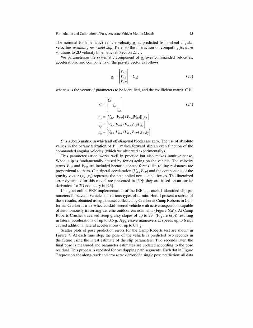
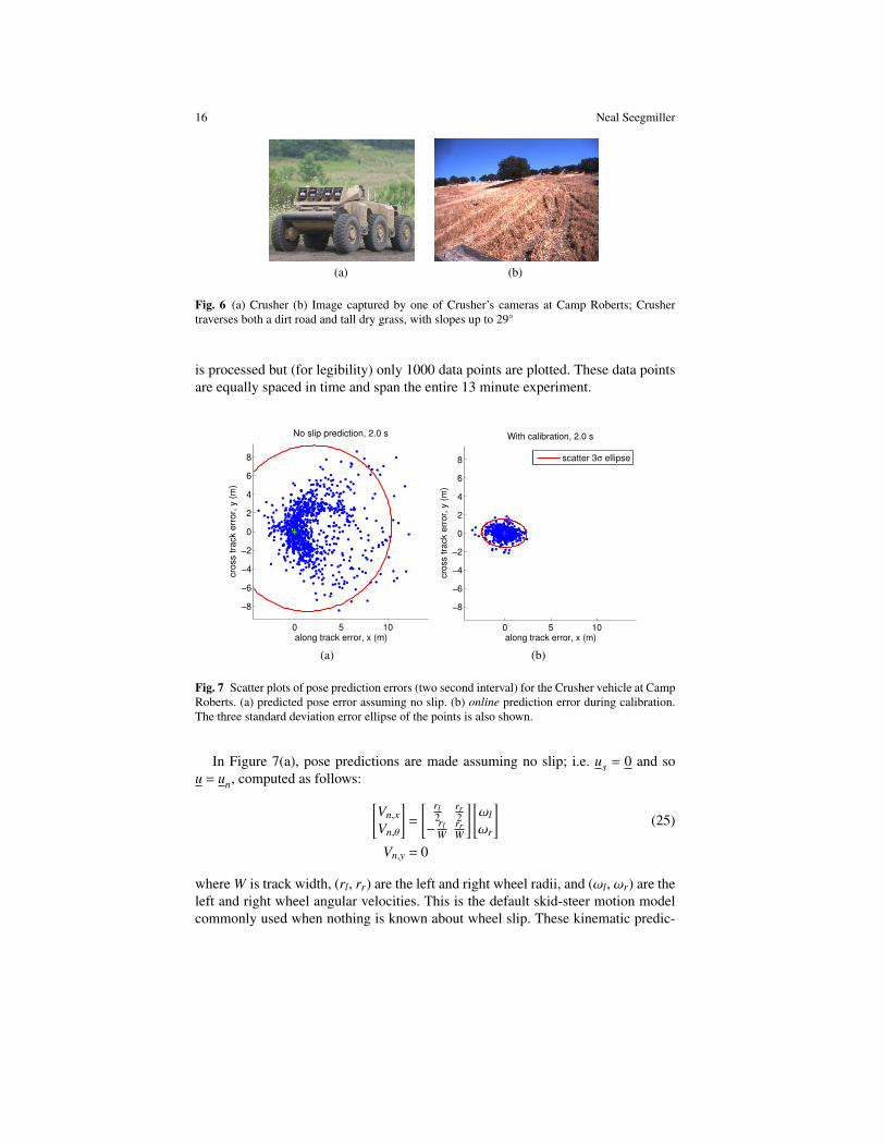
Using an online EKF implementation of the IEE approach, I identified slip pa-rameters for several vehicles on various types of terrain. Here I present a subset ofthese results, obtained using a dataset collected by Crusher at Camp Roberts in Cali-fornia. Crusher is a six-wheeled skid-steered vehicle with active suspension, capableof autonomously traversing extreme outdoor environments (Figure 6(a)). At CampRoberts Crusher traversed steep grassy slopes of up to 29◦ (Figure 6(b)) resultingin lateral accelerations of up to 0.5 g. Aggressive maneuvers at speeds up to 6 m/scaused additional lateral accelerations of up to 0.3 g.

Scatter plots of pose prediction errors for the Camp Roberts test are shown inFigure 7. At each time step, the pose of the vehicle is predicted two seconds inthe future using the latest estimate of the slip parameters. Two seconds later, thefinal pose is measured and parameter estimates are updated according to the poseresidual. This process is repeated for overlapping path segments. Each dot in Figure7 represents the along-track and cross-track error of a single pose prediction; all data

16 Neal Seegmiller

(a) (b)

Fig. 6 (a) Crusher (b) Image captured by one of Crusher’s cameras at Camp Roberts; Crushertraverses both a dirt road and tall dry grass, with slopes up to 29◦

is processed but (for legibility) only 1000 data points are plotted. These data pointsare equally spaced in time and span the entire 13 minute experiment.

0 5 10

−8

−6

−4

−2

0

2

4

6

8

No slip prediction, 2.0 s

along track error, x (m)

cro

ss t

rack e

rro

r, y

(m

)

(a)

0 5 10

−8

−6

−4

−2

0

2

4

6

8

along track error, x (m)

cro

ss tra

ck e

rror,

y (

m)

With calibration, 2.0 s

scatter 3σ ellipse

(b)

Fig. 7 Scatter plots of pose prediction errors (two second interval) for the Crusher vehicle at CampRoberts. (a) predicted pose error assuming no slip. (b) online prediction error during calibration.The three standard deviation error ellipse of the points is also shown.

In Figure 7(a), pose predictions are made assuming no slip; i.e. us = 0 and sou = un, computed as follows: [

Vn,xVn,θ

]=

[ rl2

rr2

−rlW

rrW

] [ωlωr

](25)

Vn,y = 0

where W is track width, (rl, rr) are the left and right wheel radii, and (ωl, ωr) are theleft and right wheel angular velocities. This is the default skid-steer motion modelcommonly used when nothing is known about wheel slip. These kinematic predic-

Formulation and Calibration of Fast, Accurate Vehicle Motion Models 17

tions are quite poor under conditions of steep slopes, high speeds, and persistentundersteer.

Figure 7(b) shows prediction error during online calibration with an initial es-timate of zero for all slip parameters. These calibrated predictions are significantlymore accurate. The mean error is reduced from 1.8 meters to near zero, and thestandard deviation of along track error and cross track error are reduced by 72% and83% respectively. The standard deviation of predicted heading error is reduced by90%.

The error that is not removed by the systematic calibration is accurately char-acterized by the calibrated stochastic model, as seen in Figure 8. These are scatterplots of pose prediction error just like Figure 7, but for 1, 2, and 4 second intervals.Each dot represents a path segment of unique shape for which a unique pose errorcovariance P(t) is predicted by the calibrated stochastic model according to (18).As explained in [22], the average of these predicted covariances (denoted by thedashed ellipse) is precisely the calibrated estimate of the sample covariance of theset of trajectories. The sample covariance (denoted by the solid ellipse) is computedoffline for comparison.

−4 −2 0 2 4

−5

0

5

With calibration, 1.0 s

along track error, x (m)

cro

ss tra

ck e

rror,

y (

m)

−4 −2 0 2 4

−5

0

5

With calibration, 2.0 s

along track error, x (m)

cro

ss tra

ck e

rror,

y (

m)

−4 −2 0 2 4

−5

0

5

along track error, x (m)

cro

ss tra

ck e

rror,

y (

m)

With calibration, 4.0 s

scatter 3σ

stochastic cal.

Fig. 8 Scatter plots of pose prediction error for 1, 2, and 4 second intervals. The calibrated stochas-tic model predicts a unique pose error covariance for each path segment. The dashed (green) ellipsein each plot denotes the average of these covariance predictions. The ellipses match the observedscatter of pose prediction error as it grows with time, indicating that the calibrated stochastic modelis accurate.

Notice that the calibrated stochastic model accurately predicts the changing sizeand shape of pose uncertainty in time. The elongation in the cross-track direction iscaused by the increasing effect of heading error (caused by angular velocity pertur-bations) with distance traveled.

2.2.3 IEE Applied to WMR Powertrain Calibration

The IEE approach can also be used to calibrate models of the vehicle powertrain. In acomprehensive physics-based motion model, raw inputs to vehicle motion might be

18 Neal Seegmiller

engine power or motor torque; however, for velocity kinematic models it is prefer-able if the system boundary encloses the powertrain control system (including soft-ware gains, limits, etc.). In other words, we desire a mapping from commandedangular wheel rates to actual rates.

No WMR powertrain is capable of exactly matching arbitrary wheel speed com-mands (such as step functions); doing so would require infinite torque. The dy-namics of many vehicle powertrains (and their feedback controller) can be modeledadequately by a time delay and first-order transient response:

ω(t) =1τc

(ω(t−τd)−ω(t)

)(26)

where ω denotes the angular velocity of the wheel (or engine). ω denotes the com-manded velocity, τc the time constant, and τd the time delay. Given the angularvelocity at some initial time t0 the velocity at the future time t is given by the inte-gral:

ω(t) = ω(t0) +

∫ t

t0

1τc

(ω(τ−τd)−ω(τ)

)dτ (27)

In practice this integral is computed numerically using the recursive discrete-timerelation:

ω[i + 1] = ω[i] +1τc

(ω[i−

τd

∆t]−ω[i]

)∆t (28)

where the integer in brackets [ ] denotes the time index and ∆t denotes the timestep size. If τd/∆t is not an integer, rounding or interpolation between commands isnecessary.

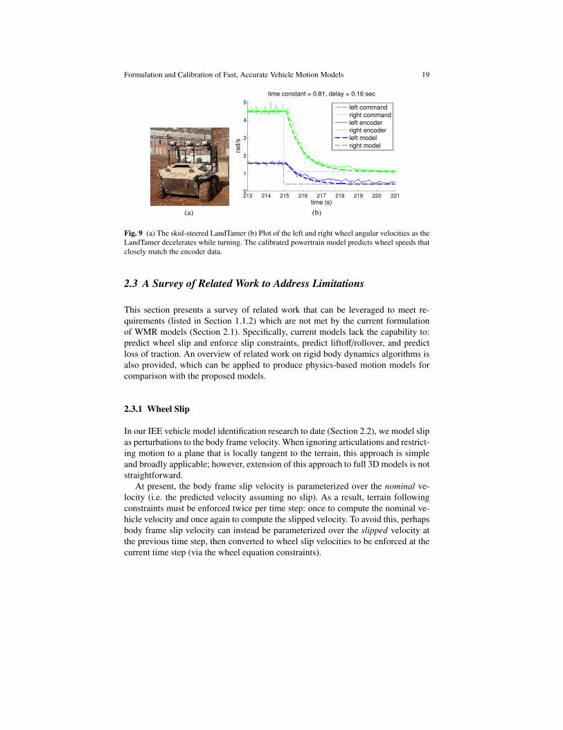
Of course more sophisticated models are possible, but experimentally this modelproved to be an adequate representation of wheel speed dynamics on Crusher, andon the hydraulic-drive LandTamer (Figure 9(a)). In one experiment, commands andwheel encoder ticks were logged as the LandTamer drove circles at various speedsand curvatures. Time constant and delay parameters were calibrated to this datasetusing an online IEE algorithm. As seen in Figure 9(b), the wheel velocities pre-dicted by the calibrated powertrain model closely match the actual wheel velocitiesmeasured by the encoders.

2.2.4 Limitations

There are important limitations to my vehicle model identification work so far. Mostimportantly, vehicle motion models used to date assume the terrain is locally planarand do not account for chassis/suspension articulations. The parameterization ofvehicle slip velocities in Section 2.2.2 performs well experimentally, but has notbeen justified in comparison to alternative models. Finally, more compelling resultsare desired demonstrating the long-term stability and real-time adaptability of theIEE calibration approach.

Formulation and Calibration of Fast, Accurate Vehicle Motion Models 19

(a)

213 214 215 216 217 218 219 220 2210

1

2

3

4

5

time constant = 0.81, delay = 0.16 sec

time (s)

rad/s

left command

right command

left encoder

right encoder

left model

right model

(b)

Fig. 9 (a) The skid-steered LandTamer (b) Plot of the left and right wheel angular velocities as theLandTamer decelerates while turning. The calibrated powertrain model predicts wheel speeds thatclosely match the encoder data.

2.3 A Survey of Related Work to Address Limitations

This section presents a survey of related work that can be leveraged to meet re-quirements (listed in Section 1.1.2) which are not met by the current formulationof WMR models (Section 2.1). Specifically, current models lack the capability to:predict wheel slip and enforce slip constraints, predict liftoff/rollover, and predictloss of traction. An overview of related work on rigid body dynamics algorithms isalso provided, which can be applied to produce physics-based motion models forcomparison with the proposed models.

2.3.1 Wheel Slip

In our IEE vehicle model identification research to date (Section 2.2), we model slipas perturbations to the body frame velocity. When ignoring articulations and restrict-ing motion to a plane that is locally tangent to the terrain, this approach is simpleand broadly applicable; however, extension of this approach to full 3D models is notstraightforward.

At present, the body frame slip velocity is parameterized over the nominal ve-locity (i.e. the predicted velocity assuming no slip). As a result, terrain followingconstraints must be enforced twice per time step: once to compute the nominal ve-hicle velocity and once again to compute the slipped velocity. To avoid this, perhapsbody frame slip velocity can instead be parameterized over the slipped velocity atthe previous time step, then converted to wheel slip velocities to be enforced at thecurrent time step (via the wheel equation constraints).

20 Neal Seegmiller

An alternative, well-precedented approach is to model the force/slip relationshipat the wheel level. In the literature, different models can be found for three distinctcases:

• Rigid wheel on rigid terrain.• Deformable wheel on rigid terrain.• Rigid wheel on deformable terrain.

The case of a rigid wheel on rigid terrain describes many indoor mobile robotswhose wheels are made of plastic or hard rubber. The standard Coulomb frictionmodel applies well in this case, in which the friction force (F f ) is limited by theproduct of the coefficient of friction (µ) and the normal force (Fn):

F f ≤ µFn (29)

A static coefficient of friction (µs) may be used when there is no relative motionbetween the wheel and ground, and a (smaller) kinetic coefficient of friction (µk)may be used when there is relative motion.

Sometimes wheels are misaligned such that satisfying all wheel equation con-straints is impossible, and one or more wheels must slip with respect to the ground.This is always the case for skid-steered vehicles when turning. When kinematic slipis unavoidable, a best fit solution is required. The pseudoinverse minimizes the mag-nitude of slip, but Alexander and Maddocks [1] propose an alternative solution thatminimizes power dissipation by friction. According to Coulomb’s law of friction,power dissipation at a wheel is proportional to the product of the slip velocity andnormal force.

The case of a deformable wheel on rigid terrain describes most automotive ap-plications, in which pneumatic tires contact paved roads. Thanks to research bythe automotive industry, empirical models relating wheel reaction forces to slip arewidely available for most tires. Brach and Brach provide a survey of these models[5] including the Bakker-Nyborg-Pacejka equations (better known as the “MagicFormula”) [36].

Figure 10 shows experimental data for a P225/60R16 tire provided by Salaani[38]; this is a representative example of the relationship between the slip and wheelreaction forces. The Magic Formula and other models capture this basic relationshipin which force is nearly linearly proportional to slip up to a peak value, above whichforce is nearly constant up to full sliding.

Finally, the case of a rigid wheel on deformable terrain describes most planetaryrover applications. Several researchers have proposed terramechanics-based modelsfor wheel contact with Lunar and Martian regolith. For example, Ishigami et al. [19]present a model which expands on earlier work by Bekker [3] and Wong & Reece[44]. In these models the normal and shear stress distribution underneath the wheeldepends on slip, sinkage, contact angle, and soil parameters such as cohesion andinternal friction angle. These stress distributions are integrated to obtain drawbarpull and normal force (illustrated in Figure 11). Ishigami et al. also provide a modelfor side force based on the bulldozing phenomenon. Iagnemma provides an approx-

Formulation and Calibration of Fast, Accurate Vehicle Motion Models 21

(a) (b)

Fig. 10 Experimental force vs. slip data for a P225/60R16 tire provided by Salaani [38]. (a) lon-gitudinal force (b) lateral force

imation of the Wong & Reece model such that soil parameters can be identifiedefficiently online [18].

Fig. 11 Free-body diagram of wheel reaction forces in deformable terrain, provided by Ishigamiet al. [19]

While these three classes of wheel/terrain interaction models are effective at mod-eling slip for their respective domains, there are challenges to integrating them withthe velocity kinematic formulation in Section 2.1.

First, all cited models require wheel reaction forces, but these are not computed invelocity kinematic simulations. We can make quasi-static assumptions and estimatewheel reaction forces using force balance equations; however, Iagnamma pointsout that the problem is underdetermined for vehicles with more than two wheels[18]. Hung et al. describe how this under-constrained problem may be formulatedas a Linear Programming or Quadratic Programming problem, given a user-definedobjective function [17].

Second, most models are formulated to compute force as a function of slip; how-ever we desire to predict slip based on force estimates. Inverting these models is

22 Neal Seegmiller

hard or impossible in closed form, because slip is not a function of force. Each slipvalue maps to exactly one force value, but each force value may map to multiple slipvalues. Slip may be a function of force over the stable region, and solutions may becomputed using the Newton-Raphson method, but this could be too slow to meetfaster-than-real-time computation requirements.

2.3.2 Liftoff/Rollover

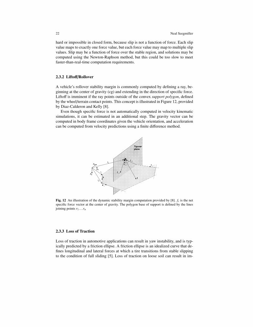
A vehicle’s rollover stability margin is commonly computed by defining a ray, be-ginning at the center of gravity (cg) and extending in the direction of specific force.Liftoff is imminent if the ray points outside of the convex support polygon, definedby the wheel/terrain contact points. This concept is illustrated in Figure 12, providedby Diaz-Calderon and Kelly [8].

Even though specific force is not automatically computed in velocity kinematicsimulations, it can be estimated in an additional step. The gravity vector can becomputed in body frame coordinates given the vehicle orientation, and accelerationcan be computed from velocity predictions using a finite difference method.

Fig. 12 An illustration of the dynamic stability margin computation provided by [8]. fr is the netspecific force vector at the center of gravity. The polygon base of support is defined by the linesjoining points r1 . . .rn

2.3.3 Loss of Traction

Loss of traction in automotive applications can result in yaw instability, and is typ-ically predicted by a friction ellipse. A friction ellipse is an idealized curve that de-fines longitudinal and lateral forces at which a tire transitions from stable slippingto the condition of full sliding [5]. Loss of traction on loose soil can result in im-

Formulation and Calibration of Fast, Accurate Vehicle Motion Models 23

mobilization and entrapment. Given soil parameters one can compute the maximumshearing force that the terrain can bear [18].

2.3.4 Rigid Body Dynamics

Fair comparison of my proposed velocity kinematic models with comprehensivephysics-based models requires that I implement the physics-based models myself.Roboticists have long required efficient algorithms for rigid body dynamics, andhave proposed numerous solutions. Featherstone provides an overview of these al-gorithms in [11] [12]. Some are for inverse dynamics (Recursive Newton-Euler Al-gorithm) and some are for forward dynamics, which suit our needs (Composite-Rigid-Body Algorithm, Articulated-Body Algorithm).

Most algorithms were developed for manipulators, but may be adaptable toWMRs. McMillan and Orin formulated a forward dynamics model for an analo-gous application, multilegged vehicles [32]. Contact between the wheels and groundcan be handled in various ways; Drumwright provides an overview in [10]. Virtualsprings may be used to apply force when objects interpenetrate, but this can be un-stable. Constraint forces may be solved for analytically by formulating the problemas a Linear Complimentarity Problem (LCP) with inequality constraints, but thiscan be computationally expensive.

In most modular implementations (such as Open Dynamics Engine) maximalcoordinates are used, meaning the state vector includes the 6 DOF pose of eachbody. Using an independent set of generalized coordinates is more difficult, butoften computationally faster. The generalized coordinates for a WMR include the 6DOF pose of the body frame and all joint angles (or lengths for prismatic joints).The CRB algorithm can be used to compute a joint space inertia matrix.

3 Research Plan

This section states the results I plan to obtain, both theoretical and experimental.These objectives build on my prior work (Section 2), and their completion shouldverify the hypothesis in Section 1.3. Limitations on scope and an itemized scheduleare also proposed.

3.1 Theoretical Objectives

I have not yet fully formulated the enhanced 3D kinematic models proposed in myhypothesis, or the process of self-calibration. Accordingly, my theoretical objectivesare to rigorously specify how to do the following.

24 Neal Seegmiller

Formulate motion prediction as the solution of a DAE in a modular way. In [39]I derived an ad hoc 3D model for the Zoe rover, but I did not provide a modularapproach that could be readily applied to other WMRs. I must provide clear steps toDAE construction for any WMR joint configuration, meaning any number of jointswith any connectivity. Joints may be rotary or prismatic and they may be driven,passive, or sprung. I must specify how to optimize solution of the DAE for efficiency,and how to resolve issues such as overconstraint. Ideally, simulating forward a singletime step should be non-iterative. A choice known to effect computation speed ischoosing the coordinate system in which calculations are performed.

Formulate and enforce slip constraints. I must specify how realistic slip con-straints should be formulated and enforced; in [39] I only enforced no-slip con-straints. Section 2.3.1 describes possible slip modeling approaches. Slip may bemodeled at the body or wheel level. Wheel slip models differ depending on the rigid-ity/deformability of the wheels and terrain. I will implement at least one version ofeach class of wheel slip model. This requires that I resolve the challenges of com-puting underdetermined wheel reaction forces and efficiently inverting force/slipmodels.

Incorporate a powertrain dynamics model. Powertrain dynamics models may beof the form in Section 2.2.3 or more complex. The powertrain model is representedby f (x,u) in the DAE, which maps commanded articulation rates to actual rates.Special steps may be required to model the delay, such as the common practice ofaugmenting the state vector with previous inputs.

Incorporate an extreme conditions predictor. I must demonstrate that the onsetof rollover and loss of traction can be accurately predicted in a velocity kinematicsimulation. My solution will leverage related work referenced in Sections 2.3.2 and2.3.3. Just like the wheel slip models, these predictors also require the estimation offorces, which are not automatically calculated in velocity kinematic simulations.

Calibrate enhanced 3D kinematic models using the integrated equation errorapproach. Prior work on IEE-based vehicle model identification (Section 2.2) usedplanar models that ignored articulations. The identification of enhanced 3D modelspresents several challenges. First, is it still possible to produce a closed-form tran-sition matrix? If not, how do we efficiently compute the Jacobian? and how do wederive the stochastic dynamics? Furthermore, I will calibrate multiple slip formula-tions that differ from prior work.

3.1.1 Deliverables

In addition to achieving the above objectives myself I desire to make my approachreadily accessible to other robotics researchers. Towards this end I plan to deliverthe following.

First, I will produce an open-source software library (written in C/C++) thatfacilitates easy construction and simulation of enhanced 3D kinematic motion mod-els. The library will be interfaced with animation software, to visualize the robot

Formulation and Calibration of Fast, Accurate Vehicle Motion Models 25

executing predicted trajectories. If appropriate (meaning real-time computationalrequirements can be met), the library may be released as a ROS package.

I will also provide, in my dissertation, a complete step-by-step explanation ofhow to construct enhanced 3D kinematic motion models for any WMR design, andhow to calibrate these models online using IEE.

3.2 Experimental Objectives

Verification of my hypothesis requires not only proving that my proposed modelformulation is feasible, but that it is superior to alternatives. I must also prove ex-perimentally that my proposed self-calibration approach performs as claimed. Ac-cordingly, my experimental objectives are to provide the following.

Quantitative comparison of the accuracy and speed of enhanced 3D kinematicmodels with alternatives. Accuracy of the models will be determined by comparingmotion predictions with data obtained in physical experiments on real vehicles. Per-haps no single platform can demonstrate the full functionality of this formulation,but most capabilities can be demonstrated by two platforms available for testing: theZoe rover and Mini Crusher.

Zoe and its next generation variant (currently in development) are uniquely artic-ulated (Figures 2, 13(a)). One of these rovers will be driven on highly uneven terrainto highlight the full 3D capability.

Mini Crusher is less articulated (having a car-like sprung suspension) but is ex-tremely fast and rugged (Figure 13(b), [35]). Mini Crusher or a similar vehicle willbe driven on slippery terrain (e.g. loose gravel) to highlight the slip modeling ca-pability. The durable Mini Crusher is also an ideal platform on which to validateliftoff/rollover prediction.

(a) (b)

Fig. 13 (a) The Zoe rover in the Atacama desert in Chile. (b) Mini Crusher. A fast, rugged, sixwheeled skid-steered vehicle with a sprung suspension. Size: 30 inches long × 20 inches wide ×12 inches high

26 Neal Seegmiller

Speed will be determined by clocking computation time for identical path pre-dictions using each model. Both comprehensive physics-based models and 2D kine-matic models will be evaluated for comparison. Resources available for comprehen-sive physics-based simulation include Open Dynamics Engine and CarSim. OpenDynamics Engine can be used to model any WMR joint configuration, but only pro-vides a friction pyramid model for wheel/terrain interaction. CarSim simulations arehigh fidelity and experimentally validated, but are limited to automobiles.

A fair comparison between my proposed velocity kinematic models and physics-based models requires that I implement the physics-based models myself. Rigidbody dynamics models will be implemented using generalized coordinates and theComposite-Rigid-Body method, as explained in Section 2.3.4. The method of pre-venting interpenetration of the wheels and terrain is yet to be determined. Givennormal force, the lateral and longitudinal wheel forces may be computed using ex-isting force/slip models (Section 2.3.1).

While I expect my proposed (first-order) kinematic models to provide equivalentaccuracy to (second-order) physics-based models under normal conditions; if tradeoffs in accuracy do exist they must be experimentally identified and quantified. AWMR motion planner using my proposed model can perhaps fall back on a slower,higher fidelity model when necessary, so long as the planner is aware of any modellimitations.

Quantitative comparison of the accuracy and speed of slip model alternatives.As explained in Section 2.3.1, the best wheel slip model is likely to be application-dependent. I will compare wheel slip models to the alternative of modeling vehicleslip in the body frame. I expect that under some conditions modeling vehicle slip isjust as accurate as modeling wheel slip, but computationally cheaper.

Experimental verification that online IEE calibration adapts quickly to chang-ing conditions, and avoids overfitting. To demonstrate adaptability, a vehicle mustbe driven on at least two distinct classes of terrain, ideally in a single continuoustest. As stated previously, overfitting depends on both the complexity of the modelformulation, and the time-variance of parameter estimates allowed by the online cal-ibration process. For example, slip parameter estimates should change when movingfrom paved to unpaved road; however, estimates should not continually change tofit noise when driving on homogeneous terrain.

3.3 Limitations on Scope

The goal of this thesis is limited to fast, accurate prediction of vehicle motion.Better understanding the physics of wheel/terrain interaction is beyond the scope

of this thesis. Our chosen wheel/terrain interaction models need not be novel, andthey may be entirely empirical as opposed to physics-based.

Likewise, making a fundamental contribution to the field of rigid body dynamicsis beyond the scope of this thesis. The primary purpose of implementing rigid bodydynamics models will be for direct comparison with the proposed velocity kinematic

Formulation and Calibration of Fast, Accurate Vehicle Motion Models 27

models. While computational optimizations will be pursued for WMR simulation,they may not be applicable to the simulation of other systems.

To ensure timely completion of this thesis, some worthwhile activities are omit-ted but may be pursued in future work.

Some advantages of the IEE calibration procedure will not be proven in this the-sis. In particular, “lifelong learning” will not be demonstrated. This would requiremonths or years of testing on the same robot to show that parameter estimates re-main stable. The use of perception (such as visual terrain classification) to aid thecalibration will also be saved for future work.

Parameters required for the prediction of extreme conditions (e.g. center of grav-ity position for rollover prevention) will not be calibrated as part of this thesis. IEEwill only be used to identify slip model parameters and dimensions (such as wheelradius during no-slip odometry calibration). These are sufficient to predict WMRmotion under normal conditions.

3.4 Schedule

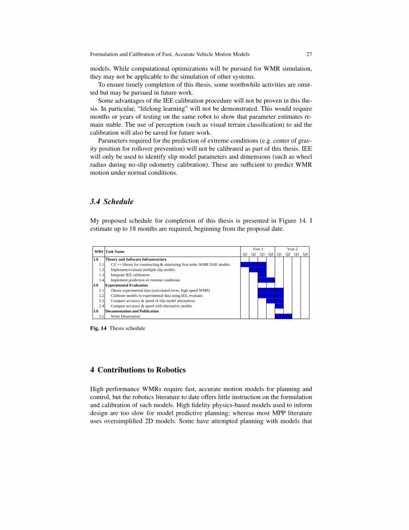
My proposed schedule for completion of this thesis is presented in Figure 14. Iestimate up to 18 months are required, beginning from the proposal date.

1.0 Theory and Software Infrastructure

1.1 C/C++ library for constructing & simulating first-order WMR DAE models

1.2 Implement/evaluate multiple slip models

1.3 Integrate IEE calibration

1.4 Implement prediction of extreme conditions

2.0 Experimental Evaluation

2.1 Obtain experimental data (articulated rover, high speed WMR)

2.2 Calibrate models to experimental data using IEE, evaluate.

2.3 Compare accuracy & speed of slip model alternatives

2.4 Compare accuracy & speed with alternative models

3.0 Documentation and Publication

3.1 Write Dissertation

Q2 Q3 Q4WBS Task Name

Year 1 Year 2

Q1 Q2 Q3 Q4 Q1

Fig. 14 Thesis schedule

4 Contributions to Robotics

High performance WMRs require fast, accurate motion models for planning andcontrol, but the robotics literature to date offers little instruction on the formulationand calibration of such models. High fidelity physics-based models used to informdesign are too slow for model predictive planning; whereas most MPP literatureuses oversimplified 2D models. Some have attempted planning with models that

28 Neal Seegmiller

compromise between fidelity and speed, but often these are derived ad hoc for aspecific WMR.

My thesis will provide an intuitive, modular approach to constructing 3D ve-locity kinematic motion models for any WMR design. In contrast to related workby Tarokh and McDermott [43], wheel velocity constraints will be derived usinga vector algebra-based approach that does not require differentiation. Furthermore,motion prediction will be formulated as the solution of a differential-algebraic equa-tion, an elegant and efficient alternative to previous nonlinear optimization-basedapproaches.

My models will account for 3D articulations on uneven terrain, and will be “en-hanced” to account for wheel slip, powertrain dynamics, and extreme conditionssuch as rollover. I predict they will provide comparable accuracy to comprehensivephysics-based models but at fraction of the computational cost, making them idealfor model predictive planning and control. These models will be suitable for any do-main, such as planetary rovers, offroad military platforms (like Crusher), automatedagricultural vehicles, self-driving cars, indoor mobile robots, etc.

Finally, building on the success of prior vehicle model identification work usingIEE, I will provide a convenient self-calibration approach for these models. Onlinecalibration of wheel/terrain interaction models will enable continuous adaptation ofwheel slip predictions to changing conditions.

Both the formulation and calibration approaches will be validated by physicalexperiments. My hope is that, whenever a roboticist requires an MPP-suitable mo-tion model for their novel WMR, they will look to my thesis first. By providing aproven, well-documented approach and open-source software tools, I aim to makethis an easy choice.

I expect this thesis to provide a foundation for future research. These motionmodels could be used for model predictive planning in complex environments, suchas when WMRs must climb over large debris in disaster sites. Planning for mobilemanipulation also requires a fast, accurate model of the mobile base.

Acknowledgments

Research to date was made with U.S. Government support under and awarded bythe Army Research Office (W911NF-09-1-0557), the Army Research Laboratory(W911NF-10-2-0016), and by the DoD, Air Force Office of Scientific Research, Na-tional Defense Science and Engineering Graduate (NDSEG) Fellowship, 32 CFR168a.

Formulation and Calibration of Fast, Accurate Vehicle Motion Models 29

Notation

⇀v means that v is a physical vector quantity expressed in coordinate system indepen-dent form. The letter r is typically used for position, v for linear velocity, and ω forangular velocity. The letter v is also used on occasion to represent a generic vector.

[⇀v]× is a skew-symmetric matrix formed from ⇀v used to represent cross productsby matrix multiplication, i.e.:

⇀a×⇀

b = [⇀a]×⇀

b =

0 −a3 a2a3 0 −a1−a2 a1 0

b1b2b3

(30)

Also note that −⇀a×⇀

b = [⇀a]T×

⇀

b⇀v

ba means the vector quantity v of frame a with respect to frame b.

cvba means the vector quantity v of frame a with respect to frame b, expressed in

the coordinates of frame c.v means that v is a vector (of any length, not necessarily a physical vector quan-

tity). f () means that the function f outputs a vector.Capital letters are typically used to denote matrices.

Definitions

IEE: (Integrated Equation Error) a method of calibrating model parameters to theintegrated dynamics of the system instead of calibrating to the differential equationdirectly. Prior work on IEE model calibration by the author includes [40] [39] [41].

MPC: (Model Predictive Control) the optimization of a single control trajectoryusing a predictive model.

MPP: (Model Predictive Planning) generalizes the notion of MPC. A diverse setof control trajectories is evaluated and the same objective function used in MPC isused to choose the best one for execution. This distinction between MPC and MPPis made in [26]

motion model: The set of equations that enables prediction of the time-evolutionof state. We propose that velocity kinematic WMR motion models are best formu-lated as a semi-explicit differential-algebraic equation (DAE), which consists of anordinary differential equation (ODE) and constraints.

motion prediction: the process of forward simulating the motion model in time,respecting constraints. In other words, solving the DAE.

pose: position and orientationself-calibration: unsupervised estimation of parameters during normal opera-

tion.velocity kinematics: In the context of WMRs, velocity kinematics are specified

by the wheel equations, which relate the velocity of the wheel/terrain contact points

30 Neal Seegmiller

to the velocity of the body frame. Velocity kinematics can be derived by taking thetime-derivative of kinematic equations, or using the vector algebra-based approachexplained in Section 2.1

WMR: wheeled mobile robot. While the term “vehicle” has a broader meaningthan “WMR” they are used interchangeably in this document.

References

1. Alexander, J.C., Maddocks, J.H.: On the kinematics of wheeled mobile robots. InternationalJournal of Robotics Research 8(5), 15–27 (1989)

2. Antonelli, G., Chiaverini, S., Fusco, G.: A calibration method for odometry of mobile robotsbased on the least-squares technique: theory and experimental validation. IEEE Transactionson Robotics 21(5), 994–1004 (2005)

3. Bekker, M.G.: Introduction to terrain-vehicle systems. The University of Michigan Press(1969)

4. Borenstein, J., Feng, L.: Measurement and correction of systematic odometry errors in mobilerobots. IEEE Transactions on Robotics and Automation 12(6), 869–880 (1996)

5. Brach, R.M., Brach, R.M.: Tire models for vehicle dynamic simulation and accident recon-struction. SAE Technical Paper 2009-01-0102 (2009)

6. Chakraborty, N., Ghosal, A.: Kinematics of wheeled mobile robots on uneven terrain. Mech-anism and Machine Theory 39(12), 1273–1287 (2004)

7. Choi, B.J., Sreenivasan, S.V.: Gross motion characteristics of articulated mobile robots withpure rolling capability on smooth uneven surfaces. IEEE Transactions on Robotics 15(2),340–343 (1999)

8. Diaz-Calderon, A., Kelly, A.: On-line stability margin and attitude estimation for dynamicarticulating mobile robots. International Journal of Robotics Research 24(10) (2005)

9. Ding, L., Yoshida, K., Nagatani, K., Gao, H., Deng, Z.: Parameter identification for planetarysoil based on a decoupled analytical wheel-soil interaction terramechanics model. In: Proc.IEEE International Conference on Intelligent Robots and Systems (2009)

10. Drumwright, E.: A fast and stable penalty method for rigid body simulation. IEEE Transac-tions on Visualization and Computer Graphics 14(1), 231–240 (2008)

11. Featherstone, R.: Robot dynamics algorithms. Kluwer Academic Publishers,Boston/Dordrecht/Lancaster (1987)

12. Featherstone, R., Orin, D.: Robot dynamics: Equations and algorithms. In: Proc. IEEE Inter-national Conference on Robotics and Automation (2000)

13. Green, C., Kelly, A.: Toward optimal sampling in the space of paths. In: Proc. InternationalSymposium on Robotics Research (2007)

14. Helmick, D., Roumeliotis, S., Cheng, Y., Clouse, D., Bajracharya, M., Matthies, L.: Slip-compensated path following for planetary exploration rovers. Advanced Robotics 20(11),1257–1280 (2006)

15. Howard, T.: Adaptive model-predictive motion planning for navigation in complex environ-ments. Carnegie Mellon University, Robotics Institute Tech. Report, CMU-RI-TR-09-32(2009)

16. Howard, T., Green, C., Ferguson, D., Kelly, A.: State space sampling of feasible motionsfor high-performance mobile robot navigation in complex environments. Journal of FieldRobotics 25(1), 325–345 (2008)

17. Hung, M.H., Orin, D.E., Waldron, K.J.: Force distribution equations for general tree-structuredrobotic mechanisms with a mobile base. In: Proc. IEEE International Conference on Roboticsand Automation (1999)

18. Iagnemma, K.: Rough-terrain mobile robot planning and control with application to planetaryexploration. Massachusetts Institute of Technology, Ph.D. Thesis (2001)

Formulation and Calibration of Fast, Accurate Vehicle Motion Models 31

19. Ishigami, G., Miwa, A., Nagatani, K., Yoshida, K.: Terramechanics-based model for steeringmaneuver of planetary exploration rovers on loose soil. Journal of Field Robotics 24(3), 233–250 (2007)

20. Ishigami, G., Nagatani, K., Yoshida, K.: Path planning and evaluation for planetary roversbased on dynamic mobility index. In: Proc. IEEE International Conference on IntelligentRobots and Systems (2011)

21. Jain, A., Guineau, J., Lim, C., Lincoln, W., Pomerantz, M., Sohl, G., Steele, R.: ROAMS: Plan-etary surface rover simulation environment. In: Proc. International Symposium on ArtificialIntelligence, Robotics and Automation in Space (2003)

22. Kelly, A.: Fast and easy systematic and stochastic odometry calibration. In: Proc. IEEE Inter-national Conference on Intelligent Robots and Systems (2004)

23. Kelly, A.: Linearized error propagation in odometry. International Journal of Robotics Re-search 23(2), 179–218 (2004)

24. Kelly, A.: A vector algebra formulation of kinematics of wheeled mobile robots. CarnegieMellon University, Robotics Institute Tech. Report, CMU-RI-TR-10-33 (2010)

25. Kelly, A., Seegmiller, N.: A vector algebra formulation of mobile robot velocity kinematics.In: Proc. Field and Service Robotics (2012)

26. Knepper, R.: On the fundamental relationships among path planning alternatives. CarnegieMellon University, Robotics Institute Tech. Report, CMU-RI-TR-11-19 (2011)

27. Lamon, P., Siegwart, R.: 3D position tracking in challenging terrain. The International Journalof Robotics Research 26(2), 167–186 (2007)

28. LaValle, S.M., Kuffner, J.J.: Randomized kinodynamic planning. International Journal ofRobotics Research 20(5), 378–400 (2001)

29. Lucet, E., Grand, C., Salle, D., Bidaud, P.: Dynamic sliding mode control of a four-wheelskid-steering vehicle in presence of sliding. In: Proc. RoManSy. Tokyo, Japan (2008)

30. Luh, J.Y.S., Walker, M.W., Paul, R.P.C.: On-line computational scheme for mechanical ma-nipulators. J. Dyn. Sys., Meas., Control 102(2), 69–76 (1980)

31. Martinelli, A., Tomatis, N., Siegwart, R.: Simultaneous localization and odometry self cali-bration for mobile robot. Autonomous Robots 22(1), 75–85 (2007)

32. McMillan, S., Orin, D.: Forward dynamics of multilegged vehicles using the composite rigidbody method. In: Proc. IEEE International Conference on Robotics and Automation (1998)

33. Mechanical Simulation Corporation: CarSim Overview. http://www.carsim.com/

products/carsim/index.php34. Muir, P.F., Neuman, C.P.: Kinematic modeling of wheeled mobile robots. Carnegie Mellon

University, Robotics Institute Tech. Report, CMU-RI-TR-86-12 (1986)35. National Robotics Engineering Center: Mini Crusher Overview. http://www.rec.ri.cmu.edu/projects/mini_crusher

36. Pacejka, H.: Tire and vehicle dynamics. SAE, Warrendale, PA (2002)37. Pivtoraiko, M., Knepper, R.A., Kelly, A.: Differentially constrained mobile robot motion plan-

ning in state lattices. Journal of Field Robotics 26(1), 308–333 (2009)38. Salaani, M.K.: Analytical tire forces and moments model with validated data. In: Proc. SAE

World Congress & Exhibition (2007). 2007-01-081639. Seegmiller, N., Rogers-Marcovitz, F., Kelly, A.: Online calibration of vehicle powertrain and

pose estimation parameters using integrated dynamics. In: Proc. IEEE International Confer-ence on Robotics and Automation (2012)

40. Seegmiller, N., Rogers-Marcovitz, F., Miller, G., Kelly, A.: A unified perturbative dynamicsapproach to vehicle model identification. In: Proc. International Symposium on RoboticsResearch (2011)

41. Seegmiller, N., Rogers-Marcovitz, F., Miller, G., Kelly, A.: Identification of vehicle modelsusing integrated equation error (2012). Submitted to: International Journal of Robotics Re-search

42. Siciliano, B., Khatib, O. (eds.): Springer Handbook of Robotics, chap. 14. Springer, Berlin,Heidelberg (2008)

43. Tarokh, M., McDermott, G.: Kinematics modeling and analyses of articulated rovers. IEEETransactions on Robotics 21(4), 539–553 (2005)

32 Neal Seegmiller

44. Wong, J.Y., Reece, A.: Prediction of rigid wheel performance based on the analysis of soil-wheel stresses. Journal of Terramechanics 4(2) (1967)

45. Yu, W., Chuy, O.Y., Collins, E.G., Hollis, P.: Analysis and experimental verification for dy-namic modeling of a skid-steered wheeled vehicle. IEEE Transactions on Robotics 26(2),340–353 (2010)

46. Yun, X., Sarkar, N.: Unified formulation of robotic systems with holonomic and nonholonomicconstraints. IEEE Transactions on Robotics 14(4), 640–650 (1998)