FAST ALGORITHM FOR EXTRACTING THE DIAGONAL OF THE …lexing/diagonal.pdf · 2018-04-18 · 758 FAST...
23
COMMUN. MATH. SCI. c 2009 International Press Vol. 7, No. 3, pp. 755–777 FAST ALGORITHM FOR EXTRACTING THE DIAGONAL OF THE INVERSE MATRIX WITH APPLICATION TO THE ELECTRONIC STRUCTURE ANALYSIS OF METALLIC SYSTEMS ∗ LIN LIN † , JIANFENG LU † , LEXING YING ‡ , ROBERTO CAR § , AND WEINAN E †¶ Abstract. We propose an algorithm for extracting the diagonal of the inverse matrices arising from electronic structure calculation. The proposed algorithm uses a hierarchical decomposition of the computational domain. It first constructs hierarchical Schur complements of the interior points for the blocks of the domain in a bottom-up pass and then extracts the diagonal entries efficiently in a top-down pass by exploiting the hierarchical local dependence of the inverse matrices. The overall cost of our algorithm is O(N 3/2 ) for a two dimensional problem with N degrees of freedom. Numerical results in electronic structure calculation illustrate the efficiency and accuracy of the proposed algorithm. Key words. Diagonal extraction, hierarchical Schur complement, electronic structure calcula- tion. AMS subject classifications. 65F30, 65Z05. 1. Introduction 1.1. Motivation The focus of this paper is fast algorithms for extracting the diagonal of the inverse of a given matrix. The particular application in our mind is electronic structure calculation, especially for models based on effective one-electron Hamiltonians such as the tight-binding models or density functional theory models. Given a matrix H, coming from the discretization of a Hamiltonian operator, one wants to evaluate ρ =2diag φ FD (H − μ) = diag 2 1+ e β(H−μ) . (1.1) Here H is the Hamiltonian given by H = − 1 2 Δ+ V (x) with a potential V (x), φ FD is the Fermi-Dirac function: φ(z)=1/(1+ e βz ), β is the inverse temperature, and μ is the chemical potential but can also be understood as a Lagrange multiplier for the constraint that the total density equals to the total number of electrons in the system: ρdx = K where K is the number of electrons in the system. Direct evaluation of (1.1) requires the diagonalization of the matrix H, and hence results in a O(N 3 ) algorithm, where N is the dimension of the matrix H. Developing algorithms with less cost has attracted a lot of attention in the past two decades. Much progress has been made for developing more efficient algorithms for insulating systems. But developing better algorithms for metallic systems has remained to be a big challenge [12]. Among the various ideas proposed, methods based on polynomial and rational expansion of the Fermi-Dirac function [1, 7, 12, 16] are particularly promising, since * Received: May 21, 2009; accepted: July 29, 2009. Communicated by Shi Jin. † Program in Applied and Computational Mathematics, Princeton University, Princeton, NJ 08544. ‡ Department of Mathematics and ICES, University of Texas at Austin, 1 University Sta- tion/C1200, Austin, TX 78712. § Department of Chemistry and Princeton Center for Theoretical Science, Princeton University, Princeton, NJ 08544. ¶ Department of Mathematics, Princeton University, Princeton, NJ 08544. 755
Transcript of FAST ALGORITHM FOR EXTRACTING THE DIAGONAL OF THE …lexing/diagonal.pdf · 2018-04-18 · 758 FAST...
COMMUN. MATH. SCI. c© 2009 International Press
Vol. 7, No. 3, pp. 755–777
FAST ALGORITHM FOR EXTRACTING THE DIAGONAL OF THE
INVERSE MATRIX WITH APPLICATION TO THE ELECTRONIC
STRUCTURE ANALYSIS OF METALLIC SYSTEMS ∗
LIN LIN† , JIANFENG LU†, LEXING YING‡ , ROBERTO CAR§ , AND WEINAN E†¶
Abstract. We propose an algorithm for extracting the diagonal of the inverse matrices arisingfrom electronic structure calculation. The proposed algorithm uses a hierarchical decomposition ofthe computational domain. It first constructs hierarchical Schur complements of the interior pointsfor the blocks of the domain in a bottom-up pass and then extracts the diagonal entries efficientlyin a top-down pass by exploiting the hierarchical local dependence of the inverse matrices. Theoverall cost of our algorithm is O(N3/2) for a two dimensional problem with N degrees of freedom.Numerical results in electronic structure calculation illustrate the efficiency and accuracy of theproposed algorithm.
Key words. Diagonal extraction, hierarchical Schur complement, electronic structure calcula-tion.
AMS subject classifications. 65F30, 65Z05.
1. Introduction
1.1. Motivation The focus of this paper is fast algorithms for extracting thediagonal of the inverse of a given matrix. The particular application in our mind iselectronic structure calculation, especially for models based on effective one-electronHamiltonians such as the tight-binding models or density functional theory models.Given a matrix H, coming from the discretization of a Hamiltonian operator, onewants to evaluate
ρ=2diagφFD(H−µ)=diag2
1+eβ(H−µ). (1.1)
Here H is the Hamiltonian given by H=− 12∆+V (x) with a potential V (x), φFD is
the Fermi-Dirac function: φ(z)=1/(1+eβz), β is the inverse temperature, and µ isthe chemical potential but can also be understood as a Lagrange multiplier for theconstraint that the total density equals to the total number of electrons in the system:∫ρdx=K where K is the number of electrons in the system.
Direct evaluation of (1.1) requires the diagonalization of the matrix H, and henceresults in a O(N3) algorithm, where N is the dimension of the matrix H. Developingalgorithms with less cost has attracted a lot of attention in the past two decades.Much progress has been made for developing more efficient algorithms for insulatingsystems. But developing better algorithms for metallic systems has remained to be abig challenge [12].
Among the various ideas proposed, methods based on polynomial and rationalexpansion of the Fermi-Dirac function [1, 7, 12, 16] are particularly promising, since
∗Received: May 21, 2009; accepted: July 29, 2009. Communicated by Shi Jin.†Program in Applied and Computational Mathematics, Princeton University, Princeton, NJ
08544.‡Department of Mathematics and ICES, University of Texas at Austin, 1 University Sta-
tion/C1200, Austin, TX 78712.§Department of Chemistry and Princeton Center for Theoretical Science, Princeton University,
Princeton, NJ 08544.¶Department of Mathematics, Princeton University, Princeton, NJ 08544.
755

756 FAST ALGORITHM FOR EXTRACTING DIAGONAL OF INVERSE MATRIX
they provide a unified framework for both insulating and metallic systems. TheFermi operator can be represented using the pole expansion (Matsubara expansion inphysical terms) [18]:
ρ=1− 4
βdiagRe
∞∑
l=1
1
(H−µ)−(2l−1)πi/β. (1.2)
The details and features of this representation will be summarized in section 3 below.Using this, the problem is reduced to evaluating the diagonal elements of a series ofinverse matrices with poles on the imaginary axis. We also remark here that a moreefficient rational approximation for the Fermi-Dirac function was recently constructedin [19].
1.2. Related work
For a typical quantum chemistry problem, the domain is taken to be a periodic box[0,n]d (d is the dimension) after normalization, V (x) is a potential that oscillates ontheO(1) scale, and µ is often on the order ofO(nd). As a result, the operator (H−µ) isfar from being positive definite. In many computations, the Hamiltonian is sampledwith a constant number of points per unit length. Therefore, the discretization of(H−µ)−(2l−1)iπ/β, denoted by M , is a matrix of dimension N =O(nd). In viewof (1.2), we are interested in extracting the diagonal of its inverse matrix G=M−1.
The most obvious algorithm is to first calculate the whole inverse matrix G, andthen extract the diagonal trivially. Of course, naive inversion leads to an algorithmthat scales as O(N3), the same as diagonalization. A better strategy would be toexplore the structure of the inverse matrix, and use an iterative method such asNewton-Schulz iteration. For an insulating system, for which it is known that thematrix elements of G decay exponentially fast away from the diagonal and hence canbe truncated, Newton-Schulz iteration gives rise to an O(N) algorithm, as was alreadydiscussed in [18]. However, such algorithms cannot be used for metallic systems sincethe elements of G decay slowly away from the diagonal. Consequently, such a trunca-tion will introduce large error. Therefore, one needs to explore other representationof the inverse matrix G.
For the case when M is a positive definite matrix, several ingenious approacheshave been developed to represent and manipulate G efficiently. One strategy is torepresent M and G using multi-resolution basis like wavelets [3, 4]. It is well knownthat for positive definiteM , the wavelet basis offers an optimally sparse representationfor both M and G=M−1. Together with the Newton-Schulz iteration, it gives riseto a linear scaling algorithm for calculating the inverse matrix G from M . In onedimension, assuming that we use L levels of wavelet coefficients and if we truncatethe matrix elements that correspond to the wavelets which are centered at locationswith distance larger than R, then the the cost of matrix-matrix multiplication isroughly O(R2L3N). In 2D, a naive extension using the tensor product structure willlead to a complexity of O(R4L6N). This has linear scaling, but the prefactor is ratherlarge: Consider a moderate situation with R=10 and L=8, R4L6 is on the order of109. This argument is rather crude, but it does reveal a paradoxical situation with thewavelet representation: although in principle linear scaling algorithms can be derivedusing wavelets, they are not practical in 2D and 3D, unless much more sophisticatedtechniques are developed to reduce the prefactor.
Another candidate for positive definite M is to use the hierarchical matrices[5, 14]. The main observation is that the off-diagonal blocks of the matrix G are
LIN LIN, JIANFENG LU, LEXING YING, ROBERTO CAR, AND WEINAN E 757
numerically low-rank and thus can be approximated hierarchically using low rankfactorizations. The cost of multiplying and inverting hierarchical matrices scales asO(N). Therefore, by either combining with the Newton-Schulz iteration, or directlyinverting the hierarchical matrices with block LU decomposition, one obtains a linearscaling algorithm.
Both of these two approaches are quite successful for M being positive definite.Unfortunately as we pointed out earlier, for the application to electronic structureanalysis, our matrix M is far from being positive definite. In fact, the matrix elementsof G are highly oscillatory due to the shift of chemical potential in the Hamiltonian.Consequently, the inverse matrix G does not have an efficient representation in eitherthe wavelet basis or the hierarchical matrix framework.
So far, we have focused our discussion on constructing the inverse matrix G.Yet another line of research is the Monte Carlo approach for extracting the diagonalusing only the matrix vector product Gv=M−1v. One algorithm of this type wasintroduced in [2]. This type of algorithm can be quite efficient if fast algorithmsfor calculating Gv are available (without the explicit knowledge of G). Examples ofsuch fast algorithms include multigrid methods [6], the fast multipole method [13](combined with iterative solvers), and the discrete symbol calculus [9], to name a few.One shortcoming of this approach is that the accuracy is relatively low for general Gdue to its Monte Carlo nature. The accuracy can be greatly improved if G is bandedor its elements decay exponentially fast away from the diagonal. However, neither ofthese conditions are satisfied for the kind of systems we are interested in.
1.3. Main observation and contribution of this work
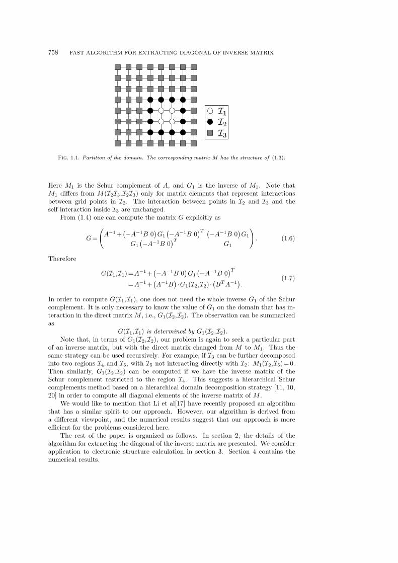
Our algorithm is based on the following observation for extracting a particularpart of the inverse matrix of a symmetric matrix M . For clarity, let us assume forthe moment that M comes from the discretization of a differential operator in a two-dimensional domain, on a grid shown in figure 1.1. Assume that the points in thedomain are indexed by I={1,··· ,N}, and I is partitioned into three disjoint setsI=I1I2I3,1 as shown in figure 1.1. The matrix elements of M between I1 and I3 arezero: M(I1,I3)=M(I3,I1)=0, i.e., M takes the form
M =
A B 0BT C D0 DT E
. (1.3)
For instance, ifM is obtained from a finite difference discretization of the Hamilto-nian operator using a five-point stencil or a tight-binding model with nearest-neighborinteraction, then M is of the form (1.3) if the domain is partitioned as in figure 1.1.
Let G=M−1. Assume that we are only interested in G(I1,I1). For instance,G(I1,I1) contains the diagonal elements of the inverse matrix for the vertices in I1.We can calculate G(I1,I1) using block Gaussian elimination:
G=
I −A−1B 00 I 00 0 I
A−1 0 000
G1
I 0 0
−BTA−1 I 00 0 I
, (1.4)
where
G1 =M−11 ,M1 =
(C DDT E
)−(BTA−1B 0
0 0
). (1.5)
1Here and in the following, we will use the notation IJ to denote the union of the two index sets
758 FAST ALGORITHM FOR EXTRACTING DIAGONAL OF INVERSE MATRIX
Fig. 1.1. Partition of the domain. The corresponding matrix M has the structure of (1.3).
Here M1 is the Schur complement of A, and G1 is the inverse of M1. Note thatM1 differs from M(I2I3,I2I3) only for matrix elements that represent interactionsbetween grid points in I2. The interaction between points in I2 and I3 and theself-interaction inside I3 are unchanged.
From (1.4) one can compute the matrix G explicitly as
G=
(A−1 +
(−A−1B 0
)G1
(−A−1B 0
)T (−A−1B 0)G1
G1
(−A−1B 0
)TG1
). (1.6)
Therefore
G(I1,I1)=A−1 +(−A−1B 0
)G1
(−A−1B 0
)T
=A−1 +(A−1B
)·G1(I2,I2) ·
(BTA−1
).
(1.7)
In order to compute G(I1,I1), one does not need the whole inverse G1 of the Schurcomplement. It is only necessary to know the value of G1 on the domain that has in-teraction in the direct matrix M , i.e., G1(I2,I2). The observation can be summarizedas
G(I1,I1) is determined by G1(I2,I2).Note that, in terms of G1(I2,I2), our problem is again to seek a particular part
of an inverse matrix, but with the direct matrix changed from M to M1. Thus thesame strategy can be used recursively. For example, if I3 can be further decomposedinto two regions I4 and I5, with I5 not interacting directly with I2: M1(I2,I5)=0.Then similarly, G1(I2,I2) can be computed if we have the inverse matrix of theSchur complement restricted to the region I4. This suggests a hierarchical Schurcomplements method based on a hierarchical domain decomposition strategy [11, 10,20] in order to compute all diagonal elements of the inverse matrix of M .
We would like to mention that Li et al[17] have recently proposed an algorithmthat has a similar spirit to our approach. However, our algorithm is derived froma different viewpoint, and the numerical results suggest that our approach is moreefficient for the problems considered here.
The rest of the paper is organized as follows. In section 2, the details of thealgorithm for extracting the diagonal of the inverse matrix are presented. We considerapplication to electronic structure calculation in section 3. Section 4 contains thenumerical results.
LIN LIN, JIANFENG LU, LEXING YING, ROBERTO CAR, AND WEINAN E 759
2. The algorithm
The algorithm for extracting the diagonal of an inverse matrix has two steps. Thefirst step is bottom-up. Starting with a hierarchical decomposition of the physical do-main, we construct the hierarchy of Schur complements by block Gaussian elimination.The idea of constructing a hierarchy of Schur complements is not new. It has beenused in the context of numerical linear algebra for quite some time. They date backto George [11] and were extended by various algorithms, e.g. multifrontal method[10, 20]. Our presentation illustrates a more geometric picture for the construction.The next step, which is new and the main contribution of this paper, is a top-downpass in which we extract the diagonal of the inverse matrix using the hierarchy ofSchur complements constructed. Here, we do not need the whole inverse matrix forthe Schur complements, but only the diagonal blocks.
We will focus on 2D systems and postpone the discussion of 3D systems to theend of this subsection.
2.1. Construction of the hierarchy of Schur complements
To explain the algorithm, we take our computational domain to be a 16×16lattice, indexed by the index set J0 (e.g., row major ordering). For the sake of clarity,we assume that the domain is partitioned into disjoint blocks hierarchically: on thetop level (Level 3), the domain is partitioned into 4 blocks, and each block is furtherdecomposed into 4 sub-blocks at the lower level. We stop at the bottom level (Level1), where the domain is partitioned into 4×4=16 blocks, as shown in figure 2.1. Amore efficient version of the algorithm actually uses blocks with shared edges and isimplemented for real calculation. We will comment on this improvement later in thissection.
2.1.1. Level 1The domain is partitioned into 4×4=16 blocks. In each block, we distinguish
“interior points” that do not interact directly with points in the other blocks, from“boundary points” that may interact with points in the other blocks. We denote byI1;ij the index set of the interior points for each block (white points in figure 2.1), andJ1;ij the index set of the boundary points of each block (black points in figure 2.1).It follows that M(I1;ij ,I1;i′j′J1;i′j′)=0 if (i,j) 6=(i′,j′).
We will use block Gaussian elimination to eliminate the interior points and reduceour problem to the boundary points only. To do so, let us permute the rows andcolumns of the matrix M such that all the interior points are ordered before theboundary points, i.e. the order of indices is changed from J0 to
J0P1−→ (I1;11I1;12 ···I1;44|J1;11J1;12 ···J1;44). (2.1)
The notation of | is used to separate interior points and boundary points. This stepis done by introducing a permutation matrix P1 such that for the matrix M definedaccording to the index set J0, and
M1 =P−11 MP1 (2.2)
is indexed according to (I1|J1). Here
I1 =I1;11I1;12 ···I1;44
is the union of all the interior points, and similarly for J1.

760 FAST ALGORITHM FOR EXTRACTING DIAGONAL OF INVERSE MATRIX
Fig. 2.1. The first level in the hierarchical domain decomposition. The interior points aredenoted as white points and boundary points are denoted as black points. The dash lines denote blocksin the decomposition (only two are shown in the figure). In this and following figures, the domainis partitioned into disjoint blocks, however, we emphasize again that in the actual implementation,we use blocks with shared edges.
Let us write M1 as
M1 =P−11 MP1 =
(A1 B1
BT1 C1
). (2.3)
The interior points that belong to different blocks do not interact with each other,and thus A1 is a block diagonal matrix.
A1 =M1(I1,I1)=
A1;11
A1;12
. . .
A1;44
(2.4)
with
A1;ij =M1(I1;ij ,I1;ij). (2.5)
Interior points inside each block only interact with the boundary points in the sameblock, hence B1 is also block diagonal:
B1 =M1(I1,J1)=
B1;11
B1;12
. . .
B1;44
(2.6)

LIN LIN, JIANFENG LU, LEXING YING, ROBERTO CAR, AND WEINAN E 761
with
B1;ij =M1(I1;ij ,J1;ij). (2.7)
We do not assume any structure for C1, and just write
C1 =M1(J1,J1). (2.8)
Since A1 is block diagonal, its inverse is given by
A−11 =
A−11;11
A−11;12
. . .
A−11;44
. (2.9)
Therefore, by Gaussian elimination, the inverse of M−11 is given by
M−11 =
(A1 B1
BT1 C1
)−1
=
(I −A−1
1 B1
0 I
)(A−1
1 00 (C1−BT
1 A−11 B1)
−1
)(I 0
−BT1 A
−11 I
).
(2.10)To simplify notation, let us denote
L1 =
(I 0
BT1 A
−11 I
). (2.11)
Since BT1 and A−1
1 are both block diagonal matrices, L1 can also be computed inde-pendently within each block, as
BT1 A
−11 =
BT1;11A
−11;11
BT1;12A
−11;12
. . .
BT1;44A
−11;44
. (2.12)
Moreover, the matrix BT1 A
−11 B1 is also block diagonal
BT1 A
−11 B1 =
BT1;11A
−11;11B1;11
BT1;12A
−11;12B1;12
. . .
BT1;44A
−11;44B1;44
. (2.13)
Using equation (2.10), we have
G=P1M−11 P−1
1 =P1LT1
(A−1
1 00 G−1
1
)L1P
−11 , (2.14)
where G1 is the Schur complement of A1, given by
G1 =(C1−BT1 A
−11 B1)
−1. (2.15)
We have now eliminated the interior points, and the problem reduces to a smallermatrix C1−BT
1 A−11 B1.
762 FAST ALGORITHM FOR EXTRACTING DIAGONAL OF INVERSE MATRIX
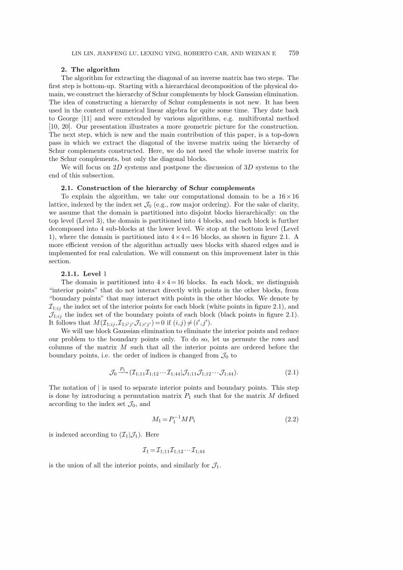
2.1.2. Level 2At the second level, the problem is to find G1, defined on the index set J1 (bound-
ary points or black points in the first level). At this level, the domain is decomposedinto 4 blocks, we again distinguish interior points with boundary points in each blockso that interior points only interact with points in the same block. As in the firstlevel, we reindex J1 by a permutation matrix P2 as
J1P2−→ (I2;11I2;12 ···I2;22|J2;11J2;12 ···J2;22)=(I2|J2). (2.16)
Here I2;ij are interior points (white points) and J2;ij are boundary points (blackpoints) inside the block (i,j) (see figure 2.2).
Fig. 2.2. The second level in the hierarchical domain decomposition. The interior points aredenoted as white points and boundary points are denoted as black points. The dash lines denoteblocks in the decomposition (only one is shown in the figure).
Following the same strategy as in the first level, denote
M2 =P−12
(C1−BT
1 A−11 B1
)P2 =
(A2 B2
BT2 C2
)(2.17)
with
A2 =M2(I2,I2), B2 =M2(I2,J2), C2 =M2(J2,J2). (2.18)
A2,B2 are block diagonal matrices (since in the first level, the update for C1 is blockdiagonal). Then
M−12 =
(A2 B2
BT2 C2
)−1
=LT2
(A−1
2 00 G2
)L2 (2.19)
LIN LIN, JIANFENG LU, LEXING YING, ROBERTO CAR, AND WEINAN E 763
with
L2 =
(I 0
BT2 A
−12 I
), G2 =(C2−BT
2 A−12 B2)
−1. (2.20)
Combining the decomposition of G1 in the second level, we obtain
G=P1LT1
A−1
1 0
0 P2LT2
(A−1
2 00 G2
)L2P
−12
L1P−11 . (2.21)
2.1.3. Level 3
At the top level, we set the interior and boundary points as shown in figure 2.3.Again, we reindex the points in J2 into I3 and J3, by a permutation matrix P3:
J2P3−→ (I3;11|J3;11)=(I3|J3). (2.22)
The final formula for G is
G=P1LT1
A−11 0
0 P2LT2
A−1
2 0
0 P3LT3
(A−1
3 00 G3
)L3P
−13
L2P−12
L1P−11 (2.23)
with
G3 =(C3−BT3 A
−13 B3)
−1. (2.24)
At the top level, G3 is inverted directly.
2.1.4. Summary of construction
In order to construct a hierarchy of Schur complements for a matrix M on adomain of size N×N , we start with a hierarchical domain decomposition scheme. Ateach level, the points inside each block are distinguished into interior and boundarypoints, so that interior points only interact with points inside the block. We reindexthe points accordingly. At each level, we eliminate the interior points. This reindexingprocedure is described as in figure 2.4.
We define for each level
Gi =
{G=M−1, i=0,
(Ci−BTi A
−1i Bi)
−1, i>0.(2.25)
The inverse of the Schur complements have the following recursive relation Gl−1 andGl as
Gl−1 =PlLTl
(A−1
l 00 Gl
)LlP
−1l . (2.26)
Using this procedure, starting from the bottom level, we can construct the hierarchyof Schur complements.
764 FAST ALGORITHM FOR EXTRACTING DIAGONAL OF INVERSE MATRIX
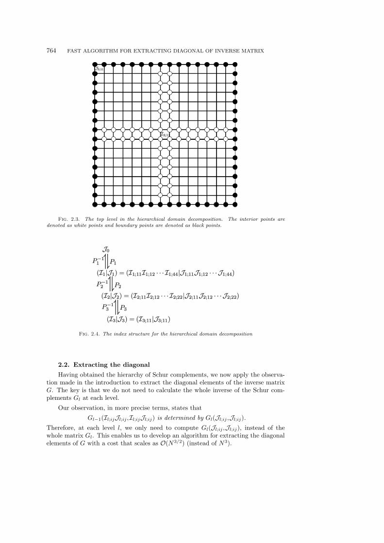
Fig. 2.3. The top level in the hierarchical domain decomposition. The interior points aredenoted as white points and boundary points are denoted as black points.
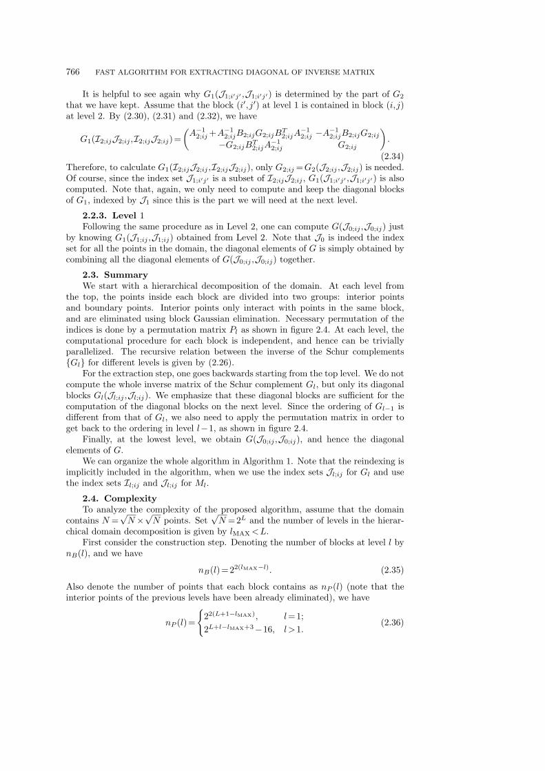
Fig. 2.4. The index structure for the hierarchical domain decomposition
2.2. Extracting the diagonal
Having obtained the hierarchy of Schur complements, we now apply the observa-tion made in the introduction to extract the diagonal elements of the inverse matrixG. The key is that we do not need to calculate the whole inverse of the Schur com-plements Gl at each level.
Our observation, in more precise terms, states that
Gl−1(Il;ijJl;ij ,Il;ijJl;ij) is determined by Gl(Jl;ij ,Jl;ij).
Therefore, at each level l, we only need to compute Gl(Jl;ij ,Jl;ij), instead of thewhole matrix Gl. This enables us to develop an algorithm for extracting the diagonalelements of G with a cost that scales as O(N3/2) (instead of N3).

LIN LIN, JIANFENG LU, LEXING YING, ROBERTO CAR, AND WEINAN E 765
2.2.1. Level 3 The extraction process starts from the top level (Level 3 in thetoy example). At the third level, given that G3 is computed directly, G2 is given bythe formula
G2 =P3LT3
(A−1
3 00 G3
)L3P
−13 =P3
(A−1
3 +A−13 B3G3B
T3 A
−13 −A−1
3 B3G3
−G3BT3 A
−13 G3
)P−1
3 .
(2.27)The matrix in the middle is indexed by (I3;11|J3;11). Due to the permutation matrixP3, G2 is indexed according to
J2 =J2;11J2;12J2;21J2;22. (2.28)
We are climbing up the ladder in figure 2.4.Since only G2(J2;ij ,J2;ij) is necessary for extracting the diagonal and we do not
need the off-diagonal blocks, we will write G2 as
G2 =
G2;11 ∗ ∗ ∗∗ G2;12 ∗ ∗∗ ∗ G2;21 ∗∗ ∗ ∗ G2;22
(2.29)
with G2;ij =G2(J2;ij ,J2;ij).
2.2.2. Level 2Proceeding to the second level, we now have
G1 =P2LT2
(A−1
2 00 G2
)L2P
−12 =P2
(A−1
2 +A−12 B2G2B
T2 A
−12 −A−1
2 B2G2
−G2BT2 A
−12 G2
)P−1
2 .
(2.30)Note that A−1
2 and B2 are all block diagonal matrices, we have
A−12 B2G2B
T2 A
−12 =
A−12;11B2;11G2;11B
T2;11A
−12;11 ∗ ∗ ∗
∗ A−12;12B2;12G2;12B
T2;12A
−12;12 ∗ ∗
∗ ∗ A−12;21B2;21G2;21B
T2;21A
−12;21 ∗
∗ ∗ ∗ A−12;22B2;22G2;22B
T2;22A
−12;22
,
(2.31)
A−12 B2G2 =
A−12;11B2;11G2;11 ∗ ∗ ∗
∗ A−12;12B2;12G2;12 ∗ ∗
∗ ∗ A−12;21B2;21G2;21 ∗
∗ ∗ ∗ A−12;22B2;22G2;22
.
(2.32)The matrix in the middle of the right hand side of (2.30) is indexed by (I2|J2).
By applying the permutation matrix P2, we climbed up another step in the ladder offigure 2.4, now G1 is indexed by
J1 =J1;11J1;12 ···J1;44, (2.33)
and we only need to keep the diagonal blocks G1(J1;ij ,J1;ij).
766 FAST ALGORITHM FOR EXTRACTING DIAGONAL OF INVERSE MATRIX
It is helpful to see again why G1(J1;i′j′ ,J1;i′j′) is determined by the part of G2
that we have kept. Assume that the block (i′,j′) at level 1 is contained in block (i,j)at level 2. By (2.30), (2.31) and (2.32), we have
G1(I2;ijJ2;ij ,I2;ijJ2;ij)=
(A−1
2;ij +A−12;ijB2;ijG2;ijB
T2;ijA
−12;ij −A−1
2;ijB2;ijG2;ij
−G2;ijBT2;ijA
−12;ij G2;ij
).
(2.34)Therefore, to calculate G1(I2;ijJ2;ij ,I2;ijJ2;ij), only G2;ij =G2(J2;ij ,J2;ij) is needed.Of course, since the index set J1;i′j′ is a subset of I2;ijJ2;ij , G1(J1;i′j′ ,J1;i′j′) is alsocomputed. Note that, again, we only need to compute and keep the diagonal blocksof G1, indexed by J1 since this is the part we will need at the next level.
2.2.3. Level 1Following the same procedure as in Level 2, one can compute G(J0;ij ,J0;ij) just
by knowing G1(J1;ij ,J1;ij) obtained from Level 2. Note that J0 is indeed the indexset for all the points in the domain, the diagonal elements of G is simply obtained bycombining all the diagonal elements of G(J0;ij ,J0;ij) together.
2.3. Summary
We start with a hierarchical decomposition of the domain. At each level fromthe top, the points inside each block are divided into two groups: interior pointsand boundary points. Interior points only interact with points in the same block,and are eliminated using block Gaussian elimination. Necessary permutation of theindices is done by a permutation matrix Pl as shown in figure 2.4. At each level, thecomputational procedure for each block is independent, and hence can be triviallyparallelized. The recursive relation between the inverse of the Schur complements{Gl} for different levels is given by (2.26).
For the extraction step, one goes backwards starting from the top level. We do notcompute the whole inverse matrix of the Schur complement Gl, but only its diagonalblocks Gl(Jl;ij ,Jl;ij). We emphasize that these diagonal blocks are sufficient for thecomputation of the diagonal blocks on the next level. Since the ordering of Gl−1 isdifferent from that of Gl, we also need to apply the permutation matrix in order toget back to the ordering in level l−1, as shown in figure 2.4.
Finally, at the lowest level, we obtain G(J0;ij ,J0;ij), and hence the diagonalelements of G.
We can organize the whole algorithm in Algorithm 1. Note that the reindexing isimplicitly included in the algorithm, when we use the index sets Jl;ij for Gl and usethe index sets Il;ij and Jl;ij for Ml.
2.4. Complexity
To analyze the complexity of the proposed algorithm, assume that the domaincontains N =
√N×√N points. Set
√N =2L and the number of levels in the hierar-
chical domain decomposition is given by lMAX<L.First consider the construction step. Denoting the number of blocks at level l by
nB(l), and we have
nB(l)=22(lMAX−l). (2.35)
Also denote the number of points that each block contains as nP (l) (note that theinterior points of the previous levels have been already eliminated), we have
nP (l)=
{22(L+1−lMAX), l=1;
2L+l−lMAX+3−16, l>1.(2.36)
LIN LIN, JIANFENG LU, LEXING YING, ROBERTO CAR, AND WEINAN E 767
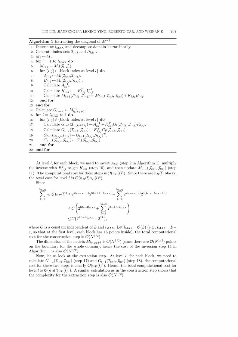
Algorithm 1 Extracting the diagonal of M−1
1: Determine lMAX and decompose domain hierarchically.2: Generate index sets Il;ij and Jl;ij .3: M1←M .4: for l = 1 to lMAX do
5: Ml+1←Ml(Jl,Jl).6: for (i,j)∈{block index at level l} do
7: Al;ij←Ml(Il;ij ,Il;ij).8: Bl;ij←Ml(Il;ij ,Jl;ij) .9: Calculate A−1
l;ij .
10: Calculate Kl;ij←−BTl;ijA
−1l;ij .
11: Calculate Ml+1(Jl;ij ,Jl;ij)←Ml+1(Jl;ij ,Jl;ij)+Kl;ijBl;ij .12: end for
13: end for
14: Calculate GlMAX←M−1
lMAX+1.15: for l = lMAX to 1 do
16: for (i,j)∈{block index at level l} do
17: Calculate Gl−1(Il;ij ,Il;ij)←A−1l;ij +KT
l;ijGl(Jl;ij ,Jl;ij)Kl;ij .
18: Calculate Gl−1(Il;ij ,Jl;ij)←KTl;ijGl(Jl;ij ,Jl;ij).
19: Gl−1(Jl;ij ,Il;ij)←Gl−1(Il;ij ,Jl;ij)T .
20: Gl−1(Jl;ij ,Jl;ij)←Gl(Jl;ij ,Jl;ij).21: end for
22: end for
At level l, for each block, we need to invert Al;ij (step 9 in Algorithm 1), multiplythe inverse with BT
l;ij to get Kl;ij (step 10), and then update Ml+1(Jl;ij ,Jl;ij) (step
11). The computational cost for these steps is O(nP (l)3). Since there are nB(l) blocks,the total cost for level l is O(nB(l)nP (l)3).
Since
lMAX∑
l=1
nB(l)nP (l)3≤22(lMAX−1)26(L+1−lMAX) +
lMAX∑
l=2
22(lMAX−l)23(L+l−lMAX+3)
≤C(
26L−4lMAX +
lMAX∑
l=2
23L+l−lMAX
)
≤C(26L−4lMAX +23L
),
where C is a constant independent of L and lMAX. Let lMAX =O(L) (e.g., lMAX =L−1, so that at the first level, each block has 16 points inside), the total computationalcost for the construction step is O(N3/2).
The dimension of the matrix MlMAX+1 is O(N1/2) (since there are O(N1/2) pointson the boundary for the whole domain), hence the cost of the inversion step 14 inAlgorithm 1 is also O(N3/2).
Now, let us look at the extraction step. At level l, for each block, we need tocalculate Gl−1(Il;ij ,Il;ij) (step 17) and Gl−1(Il;ij ,Jl;ij) (step 18), the computationalcost for these two steps is clearly O(nP (l)3). Hence, the total computational cost forlevel l is O(nB(l)nP (l)3). A similar calculation as in the construction step shows thatthe complexity for the extraction step is also O(N3/2).

768 FAST ALGORITHM FOR EXTRACTING DIAGONAL OF INVERSE MATRIX
Therefore, the total complexity for Algorithm 1 is O(N3/2). We would like toemphasize that no approximation is taken in our algorithm and all calculations areexact. Like the multifrontal algorithms, our approach relies only on the sparsitystructure of M .
So far the presentation assumes that all the blocks on the same level are disjointfrom each other. As we pointed out earlier, a more efficient version uses a decom-position in which two adjacent blocks share an edge. The modifications are fairlystraightforward, the algorithm remains almost the same, and the computational com-plexity is still O(N3/2). However, the prefactor is significantly reduced. For example,the structure of the domain decomposition on the second level now takes the formshown in figure 2.5 as opposed to figure 2.2 in the disjoint case (periodic boundarycondition is used). From figure 2.5, it is clear that the number of interior nodes tobe eliminated is roughly halved, and as a result we gain a speedup factor of 5–8 inpractice.
Fig. 2.5. The second level in the hierarchical domain decomposition using blocks with sharededges. The interior points are denoted as white points and boundary points are denoted as blackpoints. The dash lines denote blocks in the decomposition (only one is shown in the figure). Aperiodic boundary condition is assumed.
2.5. Extensions
2.5.1. Generalization to higher order finite difference stencil
The above discussion assumes that in the matrix M , a point only interacts withits nearest neighbors. In other words, the matrix M comes from a discretizationof five-point stencil. It is straightforward to extend the algorithm for higher orderstencils: at each level, for each block, there will be fewer interior points, since theinteraction range becomes longer. The computational cost will still be O(N3/2),however, the prefactor will be increased, since there will be more boundary points,and hence matrices of larger dimension.
LIN LIN, JIANFENG LU, LEXING YING, ROBERTO CAR, AND WEINAN E 769
For this reason, it is of interest to use compact stencils instead of non-compactones. For example, if a compact nine-point stencil is used, the structure of the interiorpoints will remain the same as for the five-point stencil. However, for compact stencils,the above algorithm needs some slight modifications as we discuss now.
Consider
(−∆+V )u=f. (2.37)
Denote by D5 the discretization of the Laplacian using the five-point stencil and D9
the discretization using a compact nine-point stencil (both understood as a matrix).Using the five-point stencil discretization, we have the discretized equation
D5uh +Vhuh =fh, (2.38)
where Vh is a diagonal matrix with diagonal entries given by V evaluated at the grid.The Green’s function is given by (D5 +Vh)−1, therefore, we may extract the diagonalof the discrete Green’s function using Algorithm 1. For a compact nine-point stencil,however, the discretized problem becomes
D9uh =(I+ 112D5)(−Vhuh +fh), (2.39)
or, moving uh terms to the left,
(D9 +(I+ 112D5)Vh)uh =(I+ 1
12D5)fh. (2.40)
The matrix M =D9 +(I+ 112D5)Vh has the same structure as a nine-point stencil: a
point only interacts with its surrounding eight points. However, the discrete Green’sfunction is given by M−1(I+ 1
12D5), therefore, the diagonal of the Green’s function,which is what we want, is not any more the diagonal elements of M−1, but thediagonal elements of the product matrix.
Fortunately, since the matrix I+ 112D5 is a matrix for which points only interact-
ing with their nearest-neighbors, to evaluate the diagonal of M−1(I+ 112D5), we only
need the matrix elements of M−1 that represent interaction between the grid pointswith itself (the diagonal) and with its nearest-neighbors.
Let us go back to (2.34) in the step of extracting the diagonal, note that whengoing from an upper level to a lower level, the matrix elements between the boundarypoints at the upper level will not be changed (the bottom-right block on the righthand side is still G2;ij). Therefore, the matrix elements between the boundary pointsat level l is determined by Gl, and will not be changed when we go to lower levels.
Therefore, to extract the matrix elements of G between a point with its neighbors,we still proceed in the same way as we did for extracting the diagonal. However,now at level l, if the point (say x) and one of its neighbors (say y) are both in theset of boundary points Jl, we keep the matrix elements of Gl between these twopoints. By the observation above, we have G(x,y)=Gl(x,y). At the bottom level, foreach block, we have actually calculated G(I1;ijJ1;ij ,I1;ijJ1;ij) for each block (i,j).We have obtained the elements of the inverse matrix between the points in eachblock. Therefore, for every point x, the matrix elements between that represent self-interaction and interaction with its neighbors have been calculated from the Gl weobtained at different levels, and hence, the diagonal of the matrix M−1(I+ 1
12D5) canbe calculated.
The extension to higher order compact stencil (e.g., 25-point compact stencil) isalso straightforward. The algorithm can be obtained by slight modifications of thealgorithm for higher order non-compact stencils as discussed above.

770 FAST ALGORITHM FOR EXTRACTING DIAGONAL OF INVERSE MATRIX
2.5.2. Linear scaling algorithm for elliptic problem
We can exploit additional structure of the matrices involved in the algorithm,and further reduce the computational cost. For instance, in the case that the matrixM comes from the discretization of an elliptic operator, it is known that for theintermediate matrices, the off-diagonal blocks can be approximated by a low-ranksubmatrix, known as hierarchical matrices [14] or hierarchical semi-separable matrices[8, 22]. For such matrices, the complexity of inversion and multiplication operationsis O(n), where n is the dimension of the matrix. If these approximations have beenused, the computational cost for the algorithm is reduced to O(N). Hence we obtaina linear scaling algorithm for extracting the diagonal of the inverse matrix.
2.5.3. Generalization to three dimension
For a quasi-2D system, namely, a 3D system with size√N×√N×m, where
m=O(1), it is clear that the algorithm described above can be easily generalized.We decompose the domain according to the two significant dimensions, and proceedwith hierarchical Schur complements such that the interior points are eliminated ateach level. It is not hard to see that the complexity of such an extension will still beO(N3/2) with prefactor depending on m. This would be the cost, for example, if thealgorithm is used on a Hamiltonian describing graphene sheets.
For real 3D systems with 3√N× 3√N× 3√N points (bulk system), the extension of
the algorithm starts with a hierarchical domain decomposition in three dimension: atthe top level, the domain is partitioned into 8 blocks with equal volume, and then eachblock is partitioned into 8 blocks in the lower level. The algorithm is similar to the2D algorithm, at each level, the interior points in each block are eliminated. Goingfrom the bottom level up to the top level, the problem is reduced to a problem definedon the surface of the system. Now, on the top level, the matrix M is of dimensionO(N2/3), since we have O(N2/3) points on the surface. The computational cost of thealgorithm in 3D will be O(N2). While this naive extension to 3D still has a betterscaling then the direct inversion, which costs O(N3), the gain in performance is notas substantial as in 2D.
3. Application to electronic structure
In density functional theory, at finite temperature, the system is completely deter-mined by the two-body density matrix P , which is represented by the Fermi operator
P =2
1+eβ(H−µ). (3.1)
Here β=1/kBT is the inverse temperature and µ is the chemical potential of thesystem. The factor 2 comes from spin degeneracy. The diagonal elements of P in realspace, denoted by n, is called electronic density profile, and quantifies important con-cepts such as chemical bonds etc. Another quantity of interest in electronic structureanalysis is the energy defined by
E=Tr[PH]. (3.2)
Electronic energy directly gives rise to potential energy surface for nuclei and playsan central role in ab initio quantum chemistry.
Recently, a pole expansion algorithm was proposed in [18] (also called Matsubaraexpansion in theoretical many body physics [21]) for electronic structure analysis.The Fermi operator (3.1) is represented as a sum of infinite number of poles located
LIN LIN, JIANFENG LU, LEXING YING, ROBERTO CAR, AND WEINAN E 771
on the imaginary axis
P =1− 4
βRe
∞∑
l=1
1
(H−µ)−(2l−1)πi/β. (3.3)
1/[H−µ−(2l−1)πi/β] is called the l-th pole of the Fermi operator, and the imaginarynumber µl =(2l−1)πi/β is called the Matsubara frequency. We remark that a similarexpansion is obtained in [16] based on grand canonical potential formalism. Otherrational expansions based on contour integrals, for example, those proposed in [23]and [15] can also be used in this context.
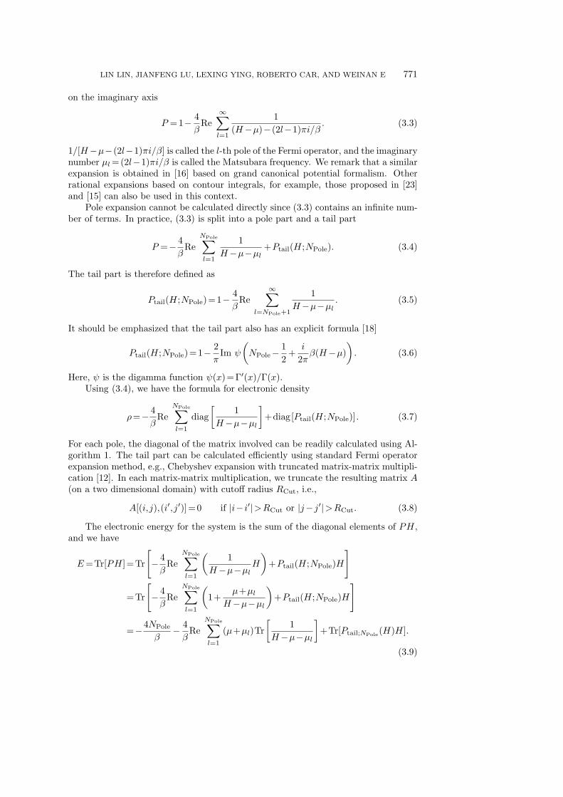
Pole expansion cannot be calculated directly since (3.3) contains an infinite num-ber of terms. In practice, (3.3) is split into a pole part and a tail part
P =− 4
βRe
NPole∑
l=1
1
H−µ−µl+Ptail(H;NPole). (3.4)
The tail part is therefore defined as
Ptail(H;NPole)=1− 4
βRe
∞∑
l=NPole+1
1
H−µ−µl. (3.5)
It should be emphasized that the tail part also has an explicit formula [18]
Ptail(H;NPole)=1− 2
πIm ψ
(NPole−
1
2+
i
2πβ(H−µ)
). (3.6)
Here, ψ is the digamma function ψ(x)=Γ′(x)/Γ(x).Using (3.4), we have the formula for electronic density
ρ=− 4
βRe
NPole∑
l=1
diag
[1
H−µ−µl
]+diag[Ptail(H;NPole)]. (3.7)
For each pole, the diagonal of the matrix involved can be readily calculated using Al-gorithm 1. The tail part can be calculated efficiently using standard Fermi operatorexpansion method, e.g., Chebyshev expansion with truncated matrix-matrix multipli-cation [12]. In each matrix-matrix multiplication, we truncate the resulting matrix A(on a two dimensional domain) with cutoff radius RCut, i.e.,
A[(i,j),(i′,j′)]=0 if |i− i′|>RCut or |j−j′|>RCut. (3.8)
The electronic energy for the system is the sum of the diagonal elements of PH,and we have
E=Tr[PH]=Tr
[− 4
βRe
NPole∑
l=1
(1
H−µ−µlH
)+Ptail(H;NPole)H
]
=Tr
[− 4
βRe
NPole∑
l=1
(1+
µ+µl
H−µ−µl
)+Ptail(H;NPole)H
]
=−4NPole
β− 4
βRe
NPole∑
l=1
(µ+µl)Tr
[1
H−µ−µl
]+Tr[Ptail;NPole
(H)H].
(3.9)
772 FAST ALGORITHM FOR EXTRACTING DIAGONAL OF INVERSE MATRIX
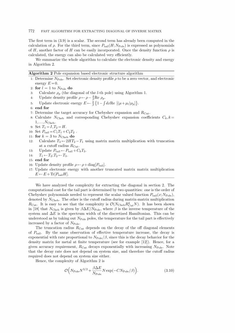
The first term in (3.9) is a scalar. The second term has already been computed in thecalculation of ρ. For the third term, since Ptail(H;NPole) is expressed as polynomialsof H, another factor of H can be easily incorporated. Once the density function ρ iscalculated, the energy can also be calculated very efficiently.
We summarize the whole algorithm to calculate the electronic density and energyin Algorithm 2.
Algorithm 2 Pole expansion based electronic structure algorithm
1: Determine NPole. Set electronic density profile ρ to be a zero vector, and electronicenergy E=0.
2: for l = 1 to NPole do
3: Calculate ρp (the diagonal of the l-th pole) using Algorithm 1.4: Update density profile ρ←ρ− 4
β Re ρp.
5: Update electronic energy E← 4β
{1−∫dxRe [(µ+µl)ρp]
}.
6: end for
7: Determine the target accuracy for Chebyshev expansion and RCut.8: Calculate NCheb and corresponding Chebyshev expansion coefficients Ck,k=
1,... ,NCheb.9: Set T1 = I,T2 =H.
10: Set Ptail =C1T1 +C2T2 .11: for k = 3 to NCheb do
12: Calculate T3←2HT2−T1 using matrix matrix multiplication with truncationat a cutoff radius RCut.
13: Update Ptail←Ptail +CkT3.14: T1←T2;T2←T3.15: end for
16: Update density profile ρ←ρ+diag[Ptail].17: Update electronic energy with another truncated matrix matrix multiplication
E←E+Tr[PtailH].
We have analyzed the complexity for extracting the diagonal in section 2. Thecomputational cost for the tail part is determined by two quantities: one is the order ofChebyshev polynomials needed to represent the scalar valued function Ptail(x;NPole),denoted by NCheb. The other is the cutoff radius during matrix-matrix multiplicationRCut. It is easy to see that the complexity is O(NChebR
4CutN). It has been shown
in [18] that NCheb is given by β∆E/NPole, where β is the inverse temperature of thesystem and ∆E is the spectrum width of the discretized Hamiltonian. This can beunderstood as by taking out NPole poles, the temperature for the tail part is effectivelyincreased by a factor of NPole.
The truncation radius RCut depends on the decay of the off diagonal elementsof Ptail. By the same observation of effective temperature increase, the decay isexponential with rate proportional to NPole/β, since this is the decay behavior for thedensity matrix for metal at finite temperature (see for example [12]). Hence, for agiven accuracy requirement, RCut decays exponentially with increasing NPole. Notethat the decay rate does not depend on system size, and therefore the cutoff radiusrequired does not depend on system size either.
Hence, the complexity of Algorithm 2 is
O(NPoleN
3/2 +β∆E
NPoleN exp(−CNPole/β)
). (3.10)
LIN LIN, JIANFENG LU, LEXING YING, ROBERTO CAR, AND WEINAN E 773
We remark that although in principle one can directly use a Chebyshev polynomialapproximation for the original Fermi operator (set NPole =0) and achieve a linearscaling algorithm, the prefactor will be quite large for metallic system. We need ahigher order Chebyshev polynomial and a larger RCut since the density matrix decaysmuch slowly (recall that RCut decays exponentially with increasing NPole). It is muchpreferable in practice to use a larger NPole. This will be further illustrated in the nextsection.
4. Numerical results
We test our algorithm on the Anderson model. The computational domain is a√N×√N lattice with periodic boundary condition. Under the nearest neighbor tight
binding approximation, the matrix components of the Hamiltonian of the system canbe written as following. All parameters are reported using atomic units.
Hi′j′;ij =
{2+Vij , i′ = i,j′ = j,
−1/2+Vij , i′ = i±1,j′ = j or i′ = i,j′ = j±1.(4.1)
The on-site potential energy Vij is chosen to be a uniform random number between0 and 10−3. The temperature is 300K. The chemical potential µ is set to satisfy thecondition that
TrP =NElectron. (4.2)
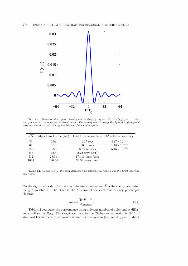
NElectron is proportional to system size. For example, for a 32×32 system, we chooseNElectron =32; therefore for a 64×64 system, NElectron =128 etc. The spectrum width∆E≈4, the inverse temperature β=1/kBT ≈1000, and hence β∆E≈4000. The ran-dom potential gives rise to an energy gap of the order 5×10⁻⁴, which is comparableto the thermal energy kBT ≈10−3. With this tiny energy gap and low temperature,the system is metallic in nature and the density matrix is a full matrix. Figure 4.1visualizes the typical behavior of density matrix for this system. The domain size is128×128. The plotted part is P (r0,r), with r0 =(1,1), and r=(1,j), j=1,... ,128. Itcan be seen that the density matrix decays slowly in the off-diagonal direction.
Table 4.1 shows the computational time and accuracy of Algorithm 1, compared tothe O(N3) scaling dense matrix inversion algorithm, which is also referred to as direct
inversion. The computations are carried out with a MATLAB code on a machine withIntel Xeon 3GHz CPU with 64GB memory. The accuracy is measured by relativeerror of the diagonal elements in L1 norm. Direct inversion clearly scales as O(N3).Algorithm 1 scales slightly better than O(N3/2). This is due to the fact that in thebottom level our algorithm is indeed O(N), and the O(N3/2) part only dominates atlarge N . Moreover, Algorithm 1 is already faster than direct inversion starting from√N =32, in which case one can gain a speedup of a factor around 35. Note that it
takes only about 3 minutes for Algorithm 1 in the case of√N =1024, while direct
inversion becomes impractical starting from√N =256.
As for accuracy, Table 4.1 shows that the error introduced by the pole part is atthe level of machine accuracy. Therefore the error for the entire algorithm comes fromthe tail part. In order to show that the tail part can also be computed effectively, wefirst test our algorithm for
√N =32.
We measure the accuracy by two quantities. One is the error of the energy perelectron defined by
∆ǫrel =|E−E|NElectron
. (4.3)
774 FAST ALGORITHM FOR EXTRACTING DIAGONAL OF INVERSE MATRIX
−64 −32 0 32 64
0
0.005
0.01
0.015
0.02
0.025
0.03
r−r0
P(r 0,r
)
Fig. 4.1. Elements of a typical density matrix P (r0,r). r0 =(1,64), r =(1,j),j =1,... ,128.r−r0 is used as x-axis for better visualization. The density matrix decays slowly in the off-diagonaldirection and this is also the typical behavior for metallic system.
√N Algorithm 1 time (sec) Direct inversion time L1 relative accuracy
32 0.03 1.07 secs 4.87×10⁻¹⁴
64 0.16 60.01 secs 1.18×10⁻¹⁴
128 0.86 3672.53 secs 5.16×10⁻¹⁴
256 4.68 2.72 days (est)512 28.61 174.11 days (est)1024 190.44 30.53 years (est)
Table 4.1. Comparison of the computational time between Algorithm 1 and the direct inversionalgorithm.
On the right hand side, E is the exact electronic energy and E is the energy computedusing Algorithm 2. The other is the L1 error of the electronic density profile perelectron
∆ρrel =Tr|P −P |NElectron
. (4.4)
Table 4.2 compares the performance using different number of poles and at differ-ent cutoff radius RCut. The target accuracy for the Chebyshev expansion is 10−5. Ifstandard Fermi operator expansion is used for this system (i.e., set NPole =0), about
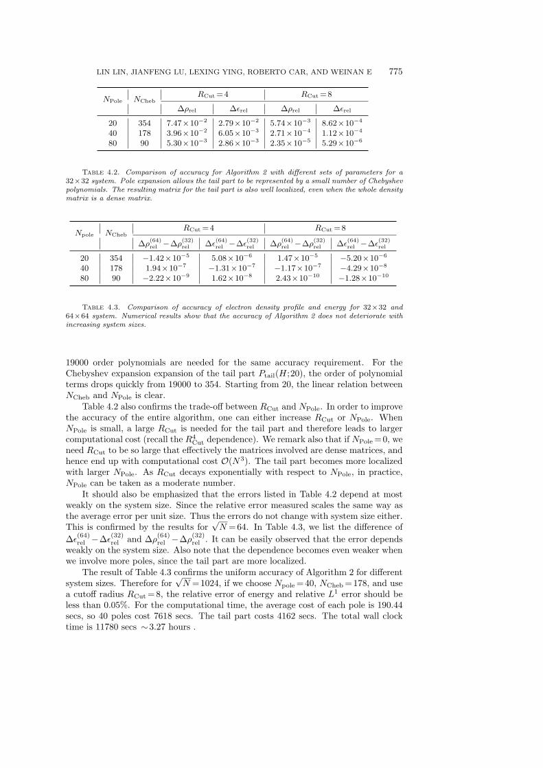
LIN LIN, JIANFENG LU, LEXING YING, ROBERTO CAR, AND WEINAN E 775
NPole NChebRCut =4 RCut =8
∆ρrel ∆ǫrel ∆ρrel ∆ǫrel
20 354 7.47×10⁻²
2.79×10⁻²
5.74×10⁻³
8.62×10⁻⁴
40 178 3.96×10⁻²
6.05×10⁻³
2.71×10⁻⁴
1.12×10⁻⁴
80 90 5.30×10⁻³
2.86×10⁻³
2.35×10⁻⁵
5.29×10⁻⁶
Table 4.2. Comparison of accuracy for Algorithm 2 with different sets of parameters for a32×32 system. Pole expansion allows the tail part to be represented by a small number of Chebyshevpolynomials. The resulting matrix for the tail part is also well localized, even when the whole densitymatrix is a dense matrix.
Npole NChebRCut =4 RCut =8
∆ρ(64)rel −∆ρ
(32)rel ∆ǫ
(64)rel −∆ǫ
(32)rel ∆ρ
(64)rel −∆ρ
(32)rel ∆ǫ
(64)rel −∆ǫ
(32)rel
20 354 −1.42×10⁻⁵
5.08×10⁻⁶
1.47×10⁻⁵
−5.20×10⁻⁶
40 178 1.94×10⁻⁷
−1.31×10⁻⁷
−1.17×10⁻⁷
−4.29×10⁻⁸
80 90 −2.22×10⁻⁹
1.62×10⁻⁸
2.43×10⁻¹⁰
−1.28×10⁻¹⁰
Table 4.3. Comparison of accuracy of electron density profile and energy for 32×32 and64×64 system. Numerical results show that the accuracy of Algorithm 2 does not deteriorate withincreasing system sizes.
19000 order polynomials are needed for the same accuracy requirement. For theChebyshev expansion expansion of the tail part Ptail(H;20), the order of polynomialterms drops quickly from 19000 to 354. Starting from 20, the linear relation betweenNCheb and NPole is clear.
Table 4.2 also confirms the trade-off between RCut and NPole. In order to improvethe accuracy of the entire algorithm, one can either increase RCut or NPole. WhenNPole is small, a large RCut is needed for the tail part and therefore leads to largercomputational cost (recall the R4
Cut dependence). We remark also that if NPole =0, weneed RCut to be so large that effectively the matrices involved are dense matrices, andhence end up with computational cost O(N3). The tail part becomes more localizedwith larger NPole. As RCut decays exponentially with respect to NPole, in practice,NPole can be taken as a moderate number.
It should also be emphasized that the errors listed in Table 4.2 depend at mostweakly on the system size. Since the relative error measured scales the same way asthe average error per unit size. Thus the errors do not change with system size either.This is confirmed by the results for
√N =64. In Table 4.3, we list the difference of
∆ǫ(64)rel −∆ǫ
(32)rel and ∆ρ
(64)rel −∆ρ
(32)rel . It can be easily observed that the error depends
weakly on the system size. Also note that the dependence becomes even weaker whenwe involve more poles, since the tail part are more localized.
The result of Table 4.3 confirms the uniform accuracy of Algorithm 2 for differentsystem sizes. Therefore for
√N =1024, if we choose Npole =40, NCheb =178, and use
a cutoff radius RCut =8, the relative error of energy and relative L1 error should beless than 0.05%. For the computational time, the average cost of each pole is 190.44secs, so 40 poles cost 7618 secs. The tail part costs 4162 secs. The total wall clocktime is 11780 secs ∼3.27 hours .
776 FAST ALGORITHM FOR EXTRACTING DIAGONAL OF INVERSE MATRIX
5. Conclusion and future work
We have proposed an algorithm for extracting the diagonal of matrices arisingfrom electronic structure calculation. Our algorithm is numerically exact and theoverall cost is O(N3/2) for a two dimensional problem with N degrees of freedom. Wehave applied our algorithm to problems in electronic structure calculations, and thenumerical results clearly illustrate the efficiency and accuracy of our approach.
We have successfully addressed problems up to one million degrees of freedom.However, many challenging problems arising from real applications involve systemswith even larger number of degrees of freedom. Therefore, one natural direction forfuture work is to develop a parallel version of our algorithm.
We have mentioned a naive extension of our algorithm to three dimensional prob-lems. However, the complexity becomes O(N2), which is not yet satisfactory. There-fore, a more challenging task is to see whether the ideas presented here can be usedto develop more efficient three dimensional algorithms.
Acknowledgement. This work was partially supported by DOE under ContractNo. DE-FG02-03ER25587 and by ONR under Contract No. N00014-01-1-0674 (L. L.,J. L. and W. E), by DOE under Contract No. DE-FG02-05ER46201 and NSF-MRSECGrant DMR-02B706 (L. L. and R. C.), and by an Alfred P. Sloan fellowship and astartup grant from the University of Texas at Austin (L. Y.). We thank LaurentDemanet from Stanford University for providing computing facility and Ming Gu andGunnar Martinsson for helpful discussions.
REFERENCES
[1] S. Baroni and P. Giannozzi, Towards very large-scale electronic-structure calculations, Euro-phys. Lett., 17, 547–552, 1992.
[2] C. Bekas, E. Kokiopoulou, and Y. Saad, An estimator for the diagonal of a matrix, AppliedNumerical Mathematics, 57, 1214–1229, 2007.
[3] G. Beylkin, R. Coifman, and V. Rokhlin, Fast wavelet transforms and numerical algorithms I,Comm. Pure Appl. Math, 44, 141–183, 1991.
[4] G. Beylkin, N. Coult, and M.J. Mohlenkamp, Fast spectral projection algorithms for density-matrix computations, J. Comput. Phys., 152, 32 – 54, 1999.
[5] S. Borm, L. Grasedyck, and W. Hackbusch, Hierarchical Matrices, Max-Planck-Institute Lec-ture Notes, 2006.
[6] A. Brandt, Multi-level adaptive solutions to boundary-value problems, Math. Comp., 31, 333–390, 1977.
[7] M. Ceriotti, T.D. Kuhne, and M. Parrinello, An efficient and accurate decomposition of theFermi operator, J. Chem. Phys, 129, 024707, 2008.
[8] S. Chandrasekaran, M. Gu, X. S. Li, and J. Xia, Superfast multifrontal method for structuredlinear systems of equations, preprint, 2007.
[9] L. Demanet and L. Ying, Discrete symbol calculus, sumbitted, 2008.[10] J.S. Duff and J.K. Reid, The multifrontal solution of indefinite sparse symmetric linear equa-
tions, ACM Trans. Math. Software, 9, 302–325, 1983.[11] J. A. George, Nested dissection of a regular finite element mesh, SIAM J. Numer. Anal., 10,
345–363, 1973.[12] S. Goedecker, Linear scaling electronic structure methods, Rev. Mod. Phys., 71, 1085–1123,
1999.[13] L. Greengard and V. Rokhlin, A fast algorithm for particle simulations, J. Comput. Phys., 73,
325–348, 1987.[14] W. Hackbusch, A sparse matrix arithmetic based on H-matrices. Part I: Introduction to H-
matrices., Computing, 62, 89–108, 1999.[15] N. Hale, N. J. Higham, and L. N. Trefethen, Computing Aα, log(A), and related matrix func-
tions by contour integrals, SIAM J. Numer. Anal., 46, 2505–2523, 2008.[16] F.R. Krajewski and M. Parrinello, Stochastic linear scaling for metals and nonmetals, Phys.
Rev. B, 71, 233105, 2005.
LIN LIN, JIANFENG LU, LEXING YING, ROBERTO CAR, AND WEINAN E 777
[17] S. Li, S. Ahmed, G. Klimeck, and E. Darve, Computing entries of the inverse of a sparsematrix using the FIND algorithm, J. Comput. Phys., 227, 9408–9427, 2008.
[18] L. Lin, J. Lu, R. Car, and W. E, Multipole representation of the Fermi operator with applicationto the electronic structure analysis of metallic systems, Phys. Rev. B, 115133, 2009.
[19] L. Lin, J. Lu, L. Ying, and W. E, Pole-based approximation of the Fermi-Dirac function,Chinese Ann. Math Ser. B (in press).
[20] J.W.H. Liu, The multifrontal method for sparse matrix solution: Theory and practice, SIAMRev., 34, 82–109, 1992.
[21] G.D. Mahan, Many-particle Physics, Plenum Pub Corp, 2000.[22] P. G. Martinsson, A fast direct solver for a class of elliptic partial differential equations, J. Sci.
Comp., 38, 316–330, 2009.[23] T. Ozaki, Continued fraction representation of the Fermi-Dirac function for large-scale elec-
tronic structure calculations, Phys. Rev. B, 75, 035123, 2007.