No 248 January 2017

Farmers’ Vulnerability to Climate Shocks: Insights from

the Niger Basin of Benin

Boris Odilon Kounagbè Lokonon

Editorial Committee

Shimeles, Abebe (Chair) Anyanwu, John C. Faye, Issa Ngaruko, Floribert Simpasa, Anthony Salami, Adeleke O. Verdier-Chouchane, Audrey

Coordinator

Salami, Adeleke O.

Copyright © 2017 African Development Bank Headquarter Building Rue Joseph Anoma 01 BP 1387, Abidjan 01 Côte d'Ivoire E-mail: afdb@afdb.org

Rights and Permissions

All rights reserved.

The text and data in this publication may be

reproduced as long as the source is cited.

Reproduction for commercial purposes is

forbidden.

Working Papers are available online at

http:/www.afdb.org/

The Working Paper Series (WPS) is produced by the

Development Research Department of the African

Development Bank. The WPS disseminates the

findings of work in progress, preliminary research

results, and development experience and lessons,

to encourage the exchange of ideas and innovative

thinking among researchers, development

practitioners, policy makers, and donors. The

findings, interpretations, and conclusions

expressed in the Bank’s WPS are entirely those of

the author(s) and do not necessarily represent the

view of the African Development Bank, its Board of

Directors, or the countries they represent.

Correct citation: Lokonon, Boris O. K. (2017), Farmers’ Vulnerability to Climate Shocks: Insights from the Niger Basin of Benin,

Working Paper Series N° 248, African Development Bank, Abidjan, Côte d’Ivoire.

Farmers’ Vulnerability to Climate Shocks: Insights from the Niger Basin of Benina

a Boris Odilon Kounagbè Lokonon is a Researcher and Lecturer at Faculté des Sciences Economiques et de Gestion (FASEG), Université de Parakou, Benin. The financial support of the German Federal Ministry of Education and Research (BMBF) through the West African Science Service Center on Climate Change and Adapted Land Use (WASCAL) research program is gratefully acknowledged. Moreover, the support of the African Development Bank (AfDB), and the African Economic Research Consortium (AERC) through the AERC/AfDB Scholars Exchange Program for Research and Mentorship Fellowship is gratefully acknowledged. The author is thankful for the support and useful comments from his mentors Dr. Adeleke O. Salami, and Professor Edwin Muchapondwa, and from the staff of the Development Research Department of the AfDB during his fellowship. The useful comments of Professor Aly A. Mbaye, Professor Joachim von Braun, Professor Kimséyinga Savadogo, and the participants of the African Economic Conference (AEC) 2015 on the earlier version of this paper are gratefully acknowledged.

AFRICAN DEVELOPMENT BANK GROUP

Working Paper No. 248

January 2017

Office of the Chief Economist

Boris Odilon Kounagbè Lokonon

4

Abstract

This paper investigates the vulnerability of farm-based livelihood systems to climate shocks in the Niger basin of Benin using a household survey dataset relative to the 2012-2013 agricultural year. The integrated approach is used to assess the vulnerability to climate shocks as function of exposure, sensitivity and adaptive capacity, and the indices are used as dependent variable in an Ordinary Least Squares regression. The findings reveal that 57.43% of the farm households are vulnerable to climate

shocks, and highlight that the lowest adaptive capacity does not necessarily coincide with highest exposure and sensitivity to result in the highest vulnerability. The econometric estimations show that vulnerability levels increase differently with respect to the type of climate shock. Floods appear to be beneficial to the farm households as they negatively influence vulnerability to climate shocks. The simulations suggest that vulnerability to climate shocks will increase, in the absence of adaptation.

Keywords: Climate shocks; Integrated approach; Niger basin of Benin; Resilience; Vulnerability.

JEL Classification: Q12, Q54.

5

1. Introduction

Climate change and variability constitutes a serious global environmental issue (Hare et al., 2011;

Vincent and Cull, 2014). Thus, the occurrence of climate shocks and extreme climatic events such

as floods, droughts, strong winds, heat waves, earthquakes, hurricanes is widespread.2 The Fifth

Assessment Report (AR5) of the Intergovernmental Panel on Climate Change (IPCC, 2014) stated

that climate shocks will likely have an overall negative effect on agricultural production in many

African countries and regions, and this could lead to food insecurity and malnutrition exacerbation.

Unlike in developed countries, agriculture in most African countries is mainly rain-fed, and

therefore is highly sensitive to climate conditions, despite its importance for these countries. For

instance, Kurukulasuriya et al. (2006) found that agricultural net revenues would fall with more

warming or drying in Africa (with temperature elasticities of -1.9 and -5.4 for dry-land crops and

livestock, respectively). However, the extent to which climate shocks affect agricultural

production differs across African regions. Roudier et al. (2011) showed that yield impact is larger

in northern West Africa (Sudano-Sahelian countries, -18% as yield impact) than in the southern

part of West Africa (Guinean countries, -13% as yield impact). These adverse impacts can lead to

the vulnerability of agriculture-dependent livelihoods, especially of smallholder farmers (Dixon et

al., 2003; IPCC, 2014).

Vulnerability to climate shocks can be exacerbated by poverty, unequal access to resources, food

insecurity, conflict, and incidence of diseases like malaria and Ebola fever (IPCC, 2014). Shocks

are basically classified in two categories (idiosyncratic and covariate shocks). Idiosyncratic shocks

are specific to each household (e.g. death of the principal income earner, chronic illness, injury,

etc.) and covariate shocks are widespread in the community (e.g. floods, droughts, strong winds,

etc.). The combination of climate and non-climatic shocks could push farmers into a poverty trap.

When caught in the poverty trap without any chance of aid (from government, non-governmental

organizations or other institutions) they can no longer escape from poverty; they are on the left

side (below) of the Micawber frontier (Carter and Barrett, 2006). Therefore, they will remain

permanently poor and vulnerable to climate shocks.

However, developing countries do not contribute as much as developed ones to the emissions of

greenhouse gases, that are the main causes of climate change which is to some extent responsible

for the increase of the probability of occurrence of climate shocks (IPCC, 2013). Thus, there is an

externality problem (Pigou, 1920).3 It is necessary to internalize the negative externalities through

relevant policies (Pigou, 1920; Coase, 1960).

Assessing the vulnerability of farm-based livelihood systems to climate shocks can help identify

and characterize actions toward strengthening their resilience, and achieve sustainable

development goals (SDGs) (Kelly and Adger, 2000; Islam et al., 2014). Indeed, one of the targets

of the first SDG is to build by 2030 the resilience of the poor and vulnerable people, and lessen

2 However, it is not easy to attribute any extreme weather event and climate shock to a change in the climate, as a

wide range of extreme events and climate shocks are expected in most regions of the world, even under unchanging

climate (IPCC, 2013). 3 Once an externality exists, there is a difference between private and social cost (Coase, 1960; Dahlman, 1979).

According to Buchanan and Stubblebine (1962), the central neo-classical critique of market organization has been,

and is externality. Even in full Pareto equilibrium, externalities may remain (Buchanan and Stubblebine, 1962).

6

their exposure and vulnerability to climate-related extreme events and other economic, social and

environmental shocks and disasters. There is a body of papers on vulnerability to climate change

and variability including climate shocks on fisheries systems (e.g. Islam et al., 2014), on

agricultural livelihoods (e.g. Brooks et al., 2005; Vincent, 2007; Shewmake, 2008; Deressa et al.,

2008; Deressa et al., 2009; Madu, 2012; Etwire et al., 2013; Simane et al., 2016) and on many

sectors of the economy (e.g. Dixon et al., 2003; Dunford et al., 2015). Three methods are

commonly used in the literature which are econometric, indicator and simulation methods.

Moreover, three major approaches of vulnerability analysis are identified in the literature: the

socio-economic, biophysical, and integrated approaches; the integrated approach combining the

socio-economic and biophysical approaches (Deressa et al., 2008). The integrated assessment can

be done, either through mapping vulnerability or computing indices, and may be theory driven or

data driven. Vulnerability indicators can be developed at country level or smaller units of analysis

(Vincent and Cull, 2014). However, there are some issues with the indicator approach; the

weighting issue, sensitivity and uncertainty issue, issue relative to the validation of the approach,

and future vulnerability issue (Vincent, 2007; Alinovi et al., 2009; Vincent and Cull, 2014).

This paper aims to assess the vulnerability of farm households to climate shocks in the Niger basin

of Benin, in order to build their resilience to these shocks using the integrated approach and an

econometric regression. The hypothesis tested in this paper is: the degree of vulnerability to

climate shocks varies significantly across different farm household characteristics, and agro-

ecological zones (AEZs). The Niger basin of Benin is chosen, because (i) Benin is located in Sub-

Saharan Africa, which is considered as the most vulnerable region to climate-related shocks (IPCC,

2014); (ii) Benin is moderately to highly vulnerable to climate shocks (Brooks et al., 2005); (iii)

the agricultural sector contributes 35% to the gross domestic product (GDP), and employs 70% of

the active population (République du Bénin, 2014); and (iv) the Niger basin covers 37.74% of

Benin land size. This paper departs from the previous studies on vulnerability to climate-related

shocks, by validating the indicator approach through a Classification and Regression Tree (CART)

model (Breiman et al., 1984), and by assessing future vulnerability through an econometric

analysis. Moreover, it adds empirical evidence to the existing literature on the quantitative analysis

of vulnerability of farm households to climate shocks in a region where such research is rare.

The remainder of the paper is organized as follow. Section 2 presents the study area. Section 3

defines vulnerability to climate shocks, discusses its relationship with resilience, and presents the

conceptual framework. Section 4 details the empirical approach, and presents variables used and

data sources. Empirical results, and their discussion are presented in section 5. Section 6 concludes.

2. Study area

The Niger basin of Benin is located in the extreme north of Benin, more specifically between

latitudes 11° and 12°30’ North and longitudes 2° and 3°20’40 East and has an area of 43,313 km2

out of the 114,763 km2 of the country (Figure 1). It belongs to the watershed of Middle Niger. The

Niger River is the largest in West Africa (4,200 km of length and a watershed of 1,125,000 km2).

The Niger basin of Benin covers five AEZs (wholly and partially) out of the eight in the country.

The communes that share the same physical, biological, and social constraints are grouped together

in one of the AEZs. Table 1 presents the characteristics of the AEZs covered by the basin, which

show the disparities across the zones in terms of climate, soils, and main crops.

Agriculture is the main activity of households in the basin. They produce for home consumption

and sell a part of their crops. The production takes place during May and November (during the

7

single rainy season). Cotton production is their main source of cash income. Farmers rely

principally on traditional agricultural systems, which are characterized by their reliance on labor

(mostly family labor) combined with limited use of improved inputs, production methods and farm

equipment. Animal traction is widespread in the eastern part of the basin due to cattle rearing.

Cattle are also kept as insurance against unexpected need, catastrophe or hardships. Small breeding

(sheep, goats, and poultry) and fisheries are also developed in the basin. Though every farm

household does not own cattle and plow for animal traction, some borrow them from their

neighbors, to deal quickly with land preparation.

Figure 1. Map of the Niger basin

Source: Author using QGIS

Pesticides are used more frequently than fertilizers. Pesticide use could be explained by cotton

production, which requires a certain quantity of insecticides. Actually, 75% of farmers in Northern

Benin use mineral fertilizers, but not for all crops (Callo-Concha et al., 2013). They use fertilizers

mainly for cotton and maize. In addition, farmers resort to manure to improve yields. Moreover,

the use of new varieties of seeds is not widespread. Irrigation is widespread only in a commune

located at the vicinity of the Niger River (Malanville), due to rice production. Furthermore, it is

hard for farmers to have access to credit outside of the cotton system. As for land ownership, the

state is the owner of land. However, the traditional ownership system is also respected (Callo-

Concha et al., 2013).

8

Table 1. Characteristics of the five agro-ecological zones of the Niger basin of Benin Agro-

ecological

zones

Climate Soil types Main crops

I Sudano-Sahelian type characterized

by a single rainy season ranging

from 700 to 900 mm per year

Ferruginous on crystalline

basement

Very fertile alluvial of the

River Niger

Millet, sorghum, cotton,

maize, rice, onion, potato

and gardening along the

Niger River

II Sudanese type characterized by a

single rainy season with annual

rainfall from 800 to 1,200 mm

Tropical ferruginous on

crystalline basement

Sorghum, maize, yam,

and cotton

III Sudanese type characterized by a

single rainy season ranging from

900 to 1,300 mm per year

Tropical ferruginous with

variable fertility and

susceptible to leaching

Yam, cotton, maize, and

cashew

IV Variation of Sudano-Sahelian to

Sudano-Guinean with annual

rainfall from 800 to 1,300 mm

Ferruginous often on deep

base with low water reserve

and scarcely fertile except the

swampy areas

Cereals in the North

coupled with yam in the

South

V Soudano-Guinean with two rainy

seasons in the South and a rainy

season in the North with annual

rainfall from 1,000 to 1,200 mm

Tropical ferruginous on

crystalline basement with very

variable characteristics

Cereals, root crops,

leguminous, and cotton

Source: Laboratory of Soil Sciences, Water and Environment (LSSEE), Center of Agricultural

Research of Agonkanmey (CRA-AG), National Agricultural Research Institute of Benin

(INRAB)

The most severe droughts that adversely affected the agricultural sector, during the past 60 years,

have occurred in 1977 and 1983. However, floods occur almost every year in the basin, and affect

farmers, especially those located at the vicinity of the Niger River. Indeed, severe floods have been

recorded in 1962, 1968, 1988, 1997, 1998, and 2010. In terms of future climate conditions,

temperature is projected to increase in the basin during the twenty first century (Hulme et al.,

2001). Rainfall is projected to increase during December-January-February, and to decrease during

June-July-August in some scenarios (Hulme et al., 2001). Therefore, the basin will likely face

difficult climate conditions and farmers will be adversely affected, if they do not adapt.

3. Background and conceptual framework

3.1 Vulnerability to climate shocks and its relationship with resilience

In economic literature (poverty and development literature), vulnerability refers to the probability

that an individual will have a level of welfare below a benchmark, at a given time in the future,

even if the person is not necessarily poor now (Hoddinott and Quisumbing, 2003; Chaudhuri,

2003; Sarris and Karfakis, 2006). It is often related to the effects of shocks such as a drought, a

drop in farm prices, or a financial crisis (Dutta et al., 2011). Three principal approaches to

assessing vulnerability are identified in economic literature: vulnerability as expected poverty

(VEP), vulnerability as low expected utility (VEU), and vulnerability as uninsured exposure to

risk (VER), sharing a common characteristic which is to construct a model that predicts a measure

of welfare (Hoddinott and Quinsumbing, 2003). VEP and VEU are ex ante assessments which

share two further common characteristics; they use a reference benchmark for the welfare

9

indicator, and enumerate a likelihood of falling below this benchmark (Hoddinot and Quisumbing,

2003; Sarris and Karfakis, 2006). VER is an ex post assessment as it does not construct likelihoods;

it assess the extent to which observed shocks generate welfare losses.

VEP is defined as the probability that the household’s welfare in the future will be below a given

benchmark (for example the consumption poverty line) (Hoddinott and Quisumbing, 2003; Sarris

and Karfakis, 2006). Similarly, VEU is defined as the difference between the utility derived from

some level of certainty-equivalent consumption at and above which the household would not be

considered vulnerable and the expected utility of consumption (Hoddinott and Quisumbing, 2003;

Sarris and Karfakis, 2006). As for VER, it is an assessment of the extent to which a negative shock

causes a welfare loss (Hoddinot and Quisumbing, 2003).

However, there are other way to define vulnerability, especially vulnerability to climate shocks.

Vulnerability of farm-based livelihoods to climate shocks can be defined as the propensity or

predisposition they are to be adversely affected (adapted from IPCC, 2014, p. 1775). Vulnerability

of farm-based livelihood systems encompasses a variety of concepts and elements including

sensitivity or susceptibility to climate shocks, and lack of capacity to cope and adapt (adapted from

IPCC, 2014, p. 1775). It is function of exposure, sensitivity, and adaptive capacity.

Exposure in the IPCC framework has an external dimension, whereas both sensitivity and adaptive

capacity have an internal dimension (Füssel, 2007). Therefore, to assess the vulnerability of farm-

based livelihood systems to climate shocks, it is necessary to understand each of the three

components of vulnerability. Indeed, exposure in the context of this paper is the presence of farm-

based livelihood systems in places and settings that could be adversely affected (adapted from

IPCC, 2014, p. 1765). Exposure indicators characterize the frequency of extreme events, scale of

land erosion and sea-level rise, and changes in temperature and rainfall (Islam et al., 2014).

Sensitivity in this paper is the degree to which a farm-based livelihood system is affected, either

adversely or beneficially, by climate shocks (adapted from IPCC, 2014, p. 1772). Sensitivity does

not mean only negative effect, but includes also positive one, because the occurrence of climate

shocks may be beneficial to some farm-based livelihood systems. Adaptive capacity is the ability

of farm-based livelihood system to adjust to climate shocks, to take advantage of opportunities, or

to respond to consequences (adapted from IPCC, 2014, p. 1758).

In the IPCC framework, adaptive capacity is negatively related to vulnerability. More adaptive

capacity means lesser vulnerability to climate shocks in this framework. However, high adaptive

capacity cannot be always associated with lesser vulnerability. A farm-based livelihood system

may have high adaptive capacity and may end up being adversely affected by climate shocks,

leading to high vulnerability. Moreover, low adaptive capacity can result to lesser vulnerability.

Indeed, as sensitivity includes also positive effect of climate shocks, some farmers can benefit

from these shocks.

Vulnerability has a negative connotation. Thus, the analyses include resilience as it is becoming

influential in development and vulnerability reduction (Béné et al., 2012). It is worth noting that

the concept of resilience originated in ecology (Holling, 1973). Resilience is the capacity of farm-

based livelihood system to cope with climate shocks, responding or reorganizing in ways that

maintain its essential function, identity, and structure, while also maintaining the capacity for

adaptation, learning, and transformation (adapted from IPCC, 2014, p. 1772). It can also be defined

as the capacity of a farm-based livelihood system to absorb disturbances and reorganize, while

10

undergoing change so as to retain essentially the same function, structure, identity and feedback

(adapted from Resilience Alliance, 2010, p. 51).

There is a relationship between vulnerability and resilience (Schoon, 2005; Engle, 2011; Béné et

al., 2012). Adaptive capacity, which is one of the three components of vulnerability, is influenced

by resilience as illustrated by Figure 2 (Klein et al., 2003; Adger, 2006; Engle, 2011). A farm-

based livelihood system lacks resilience, as it is vulnerable, and is vulnerable due to lack of

resilience (Klein et al., 2003). The relationship between vulnerability and resilience is not only

through adaptive capacity. An important feature of resilience is its consideration of the dynamic

aspects of vulnerability, as resilience refers to the ability of a farm-based livelihood system to

return to an earlier stable state, after a climate shock (Füssel, 2007). Analyzing the Resilience

Alliance’s definition of vulnerability, Füssel (2007) referred to vulnerability as the antonym of

resilience. He also argued that the second aspect of the Resilience Alliance’s definition of

vulnerability, which considers vulnerability as function of exposure, sensitivity, and resilience

owing to adaptive capacity seems to be incompatible with the first one.4

Figure 2. Vulnerability and resilience frameworks as linked through adaptive capacity

Source: Adapted from Engle (2011)

3.2 Conceptual framework

The vulnerability (v) level at period t is a function of exposure variables Ev, sensitivity variables

Sv, adaptive capacity variables ACv, v levels of the periods t − j and unobservable characteristics

including measurement errors and innate v, μt:

vt = f(Ev,t, Sv,t, ACv,t, vt−j, μt), j = 1, 2, … , T (1)

As adaptive capacity is composed of five kinds of capital: physical, institutional capital and

technology (PC), human capital (HC), natural capital (NC), financial capital (FC) and social capital

(SC) based on the Sustainable Livelihoods framework (Scoones, 1998), equation 1 becomes:

vt = f(Ev,t, Sv,t, PCv,t, HCv,t, NCv,t, FCv,t, SCv,t, vt−j, μt), j = 1, 2, … , T (2)

The financial capital variables include income from farming and from off-farm activities.

Therefore, they have to come from the maximization of household utility. It is assumed for

4 As a farmer can be very poor and unwell, but very resilient, resilience alone is not sufficient when referring to

climate and development (Béné et al., 2012).

11

simplicity that vulnerability level depends on current household incomes, though a portion of

income serves as consumption in the following period.

Assuming that they are 𝑛 members within the household, consumption and leisure of each member

at period 𝑡 are respectively 𝑐𝑖,𝑡 𝑎𝑛𝑑 𝑙𝑖,𝑡, 𝑓𝑜𝑟 𝑖 = 1, 2, … , 𝑛. The Agricultural Household Model has

two components (Benjamin, 1992). Firstly, a twice differentiable, quasi-concave utility function

defined over consumption, and leisure: 𝑢ℎ,𝑡 = 𝑢(𝑐𝑡 = ∑ 𝑐𝑖,𝑡𝑛𝑖=1 , 𝑙𝑡 = ∑ 𝑙𝑖,𝑡

𝑛𝑖=1 ; 𝑎𝑡), with ℎ being

the index of the households. The utility function is parameterized by the vector 𝑎𝑡, which

summarizes household characteristics at a given period 𝑡. Secondly, a twice differentiable simple,

concave production function: 𝑄𝑡 = 𝐹𝑡(𝐿𝑡; 𝐴𝑡), where 𝐿𝑡 is labor (the sum of family and hired labor,

𝐿𝑡 = 𝐿𝑡𝐹 + 𝐿𝑡

𝐻; where 𝐿𝑡𝐹 = ∑ 𝛼𝑖 × 𝐿𝑖,𝑡

𝐹𝑛𝑖=1 and 𝐿𝑡

𝐻 = ∑ 𝛿𝑘 × 𝐿𝑘,𝑡𝐻𝑚

𝑘=1 ), and land 𝐴𝑡 is assumed fixed

and exogenous. (𝛼𝑖, 𝛿𝑘) ∈ (0, 1] × (0, 1] and accounts for the heterogeneity of family and hired

labor; it is assumed that the household can hire 𝑚 categories of labor (e.g., men, women, etc.).

𝐹𝑡: 𝑅+ → 𝑅+, 𝐹𝑡′(𝐿𝑡; 𝐴𝑡) > 0 and 𝐹𝑡

′′(𝐿𝑡; 𝐴𝑡) < 0 for all 𝐿𝑡 > 0, lim𝐿𝑡→0

𝐹𝑡′(𝐿𝑡; 𝐴𝑡) = ∞ and

lim𝐿𝑡→∞

𝐹𝑡′(𝐿𝑡; 𝐴𝑡) = 0.

Each household member could work on the family farm and/or could look for off-farm activities.

The prices of hired labor 𝐿𝑡𝐻 and off-farm labor 𝐿𝑡

𝑂 are assumed to be equal to 𝑤𝑡. The time

endowment of the household is 𝑇𝑡(𝑎𝑡) = ∑ 𝛼𝑖 × 𝑇𝑖,𝑡𝑛𝑖=1 and its exogenous income is 𝑦𝑡. The

exogenous income includes any kind of assistance from friends, relatives and remittances. All

prices are normalized by the output price. The farm household allocates its time endowment

between leisure, work on the farm, and work off the farm. It is also possible for the farm household

to hire labor to produce output that is sold in a competitive market. Thus, the farm household’s

problem is:

𝑀𝑎𝑥 𝑢(𝑐𝑡 = ∑ 𝑐𝑖,𝑡𝑛𝑖=1 , 𝑙𝑡 = ∑ 𝑙𝑖,𝑡

𝑛𝑖=1 ; 𝑎𝑡) (3)

with respect to 𝑐𝑡, 𝑙𝑡, 𝐿𝑡𝑂 , 𝐿𝑡

𝐻, 𝐿𝑡𝐹 subject to

𝑐𝑡 = 𝐹𝑡(𝐿𝑡; 𝐴𝑡) + (−𝑤𝑡 × 𝐿𝑡𝐻 + 𝑤𝑡 × 𝐿𝑡

𝑂 + 𝑦𝑡), (4)

𝑙𝑡 + 𝐿𝑡𝐹 + 𝐿𝑡

𝑂 = 𝑇𝑡(𝑎𝑡) (5)

𝐿𝑡𝐹 + 𝐿𝑡

𝐻 = 𝐿𝑡 (6)

Collapsing the three constraints into a single constraint yields:

𝑐𝑡 + 𝑤𝑡 × 𝑙𝑡 = 𝑦𝑡 + 𝜌𝑡(𝑤𝑡; 𝐴𝑡) + 𝑤𝑡 × 𝑇𝑡(𝑎𝑡) ≡ 𝑌𝑡. (7)

Consumption of goods and leisure at period 𝑡 equals full income 𝑌𝑡 that is composed of exogenous

income 𝑦𝑡, value of time endowment 𝑤𝑡 × 𝑇𝑡(𝑎𝑡), and non-maximized farm profits

𝜌𝑡(𝑤𝑡; 𝐴𝑡) = 𝐹𝑡(𝐿𝑡; 𝐴𝑡) − (𝑤𝑡 × 𝐿𝑡𝐻 + 𝑤𝑡 × 𝐿𝑡

𝐹).

In the case separation holds, the problem will be solved recursively. First, the household will

maximize profit at each period, and then utility. Profit maximization yields the household labor

demand:

12

𝐿𝑡∗ = 𝐿𝑡

∗(𝑤𝑡, 𝐴𝑡) (8)

Thus, the optimal profit is:

𝜌𝑡∗ = 𝜌𝑡

∗(𝑤𝑡, 𝐴𝑡) (9)

The maximization of utility yields:

𝑙𝑡∗ = 𝑙𝑡

∗(𝑤𝑡, 𝑌𝑡; 𝑎𝑡) (10)

Thus, the household labor supply (work on the farm and work off of the farm) is given by:

𝐿𝑡𝑆(𝑤𝑡, 𝑌𝑡; 𝑎𝑡) = 𝑇𝑡(𝑎𝑡) − 𝑙𝑡

∗ (11)

Hence, equation 2 becomes:

𝑣𝑡 = 𝑓(𝐸𝑣,𝑡, 𝑆𝑣,𝑡, 𝑃𝐶𝑣,𝑡, 𝐻𝐶𝑣,𝑡, 𝑁𝐶𝑣,𝑡, 𝐹𝐶𝑣,𝑡′ , 𝑆𝐶𝑣,𝑡

′ , 𝜌𝑡∗, 𝑦𝑡, 𝑤𝑡 × 𝑙𝑡

∗, 𝑤𝑡 × 𝐿𝑡𝐹∗, 𝑤𝑡 × 𝐿𝑡

𝑂∗, 𝑣𝑡−𝑗 , 𝜇𝑡), 𝑗 =

1, 2, … , 𝑇 (12)

where 𝐹𝐶𝑣,𝑡′ are financial capital variables except incomes from farming and from off-farm

activities, and 𝑆𝐶𝑣,𝑡′ are social capital variables except any kind of assistance from friends and

relatives.

𝑣𝑡 is assumed to be increasing in the adaptive capacity variables, and decreasing in the exposure

and sensitivity variables. Therefore, a policy-maker that aims to minimize the vulnerability level

of the household should implement either policies which will decrease exposure or sensitivity, or

which will strengthen adaptive capacity.

4. Empirical approach, description of the variables, and data

4.1 Empirical approach

Equation 12 is used to assess vulnerability to climate shocks. Vulnerability index is calculated as

the net effect of adaptive capacity, sensitivity and exposure:

𝑣 = 𝑎𝑑𝑎𝑝𝑡𝑖𝑣𝑒 𝑐𝑎𝑝𝑎𝑐𝑖𝑡𝑦 − (𝑒𝑥𝑝𝑜𝑠𝑢𝑟𝑒 + 𝑠𝑒𝑛𝑠𝑖𝑡𝑖𝑣𝑖𝑡𝑦). (13)

One of the features of the indicator approach is to assign a weight to each indicator. Thus, two

alternatives may be used: either to give them equal weight or to assign different weights, to avoid

the uncertainty of equal weighting given the diversity of indicators used (Deressa et al., 2008).

This paper adopts the different weighting alternative using dimension reduction methods; Principal

Component Analysis (PCA), and Factor Analysis (FA) (Pearson, 1901; Spearman, 1904). Each

continuous indicator of the components of vulnerability is normalized before running PCA and

FA, using Z-Score standardization:

𝑋𝑖∗ =

𝑋𝑖−𝑀𝑖(𝑋)

𝑆𝐷𝑖(𝑋) (14)

where 𝑋𝑖∗ is a normalized value of a continuous indicator of a farm household; 𝑋𝑖 and 𝑆𝐷𝑖(𝑋) are

the actual value and the standard deviation of the same indicator respectively. The indicators were

normalized, because they were measured on different scales. Regarding adaptive capacity, the

13

variables ‘distance from dwelling to drinking water source’ and ‘distance from dwelling to paved

or tarred road’ are considered as costs. Therefore, the negatives of their Z-scores are used.

As vulnerability is a multi-dimensional concept (Vincent and Cull, 2014), all the extracted

components from PCA and FA are used in computing the sub-indices. Each component from PCA

and FA is weighted by its percentage of explained variance. Suppose 𝑝 components are extracted,

for each indicator equation (15) is employed, before building the sub-indices:

𝑌𝑖∗ =

𝑉𝑎𝑟𝑗

∑ 𝑉𝑎𝑟𝑗𝑝𝑗=1

× 𝐹𝑎𝑐𝑡𝑜𝑟𝑗𝑖 × 𝑋𝑖∗, 𝑓𝑜𝑟 𝑎𝑙𝑙 𝑐𝑜𝑚𝑝𝑜𝑛𝑒𝑛𝑡 𝑗 (15)

where 𝑉𝑎𝑟𝑗 is the percentage of explained variance of the component j and 𝐹𝑎𝑐𝑡𝑜𝑟𝑗𝑖 is the jth

factor score relative to the ith indicator.

Vulnerability index is computed for each farm household using equation (16).

𝑣ℎ = ∑ ∑𝑉𝑎𝑟𝑗

∑ 𝑉𝑎𝑟𝑗𝑝𝑗=1

∗ 𝐹𝑎𝑐𝑡𝑜𝑟𝑗𝑖 ∗ 𝑋𝑎𝑖∗ − (∑ ∑

𝑉𝑎𝑟𝑗

∑ 𝑉𝑎𝑟𝑗𝑝𝑗=1

∗ 𝐹𝑎𝑐𝑡𝑜𝑟𝑗𝑖 ∗ 𝑋𝑒𝑖∗ +𝑝

𝑗=1𝑛𝑒𝑖=1

𝑝𝑗=1

𝑛𝑎𝑖=1

∑ ∑𝑉𝑎𝑟𝑗

∑ 𝑉𝑎𝑟𝑗𝑝𝑗=1

∗ 𝐹𝑎𝑐𝑡𝑜𝑟𝑗𝑖 ∗ 𝑋𝑠𝑖∗𝑝

𝑗=1𝑛𝑠𝑖=1 ) (16)

where 𝑋𝑎𝑖∗ , 𝑋𝑒𝑖

∗ , and 𝑋𝑠𝑖∗ are the Z-Score standardizations of adaptive capacity, exposure, and

sensitivity variables, respectively. 𝑛𝑎, 𝑛𝑒, and 𝑛𝑠 represent the number of adaptive capacity,

exposure, and sensitivity variables, respectively.

Two of the key issues of the indicator method are relative to its validation, and future vulnerability

assessment (Vincent, 2007; Alinovi et al., 2009; Vincent and Cull, 2014). Alinovi et al. (2009)

argued that to assess the meaningfulness of the procedure used for computing indices, a CART

model may be used. Therefore, the paper uses a CART model to estimate the vulnerability decision

tree and related splitting rules. CART model aids the researcher in choosing from many potentially

relevant variables, and by suggesting refinements in functional form that are appropriate in

subsequent parametric analysis (Larose, 2005). As the target variable is continuous (vulnerability

index5), CART will create a regression tree. The original indicators that are used for the

computation of vulnerability index are employed in the CART analysis.

An econometric analysis is performed to find the main factors that can significantly lessen the

vulnerability to climate shocks among those used to build the index and for simulation purposes.

This is due to the major limitation of the indicator method, as it always produce normalized

indicators with means zero, so it is difficult to compare the level of vulnerability over time (Alinovi

et al., 2009). The vulnerability equation is specified as follows:

𝑣ℎ = 𝛽0 + 𝑋ℎ𝛽 + 𝛾ℎ (19)

where 𝑋ℎ is the set of variables belonging to the three dimensions of vulnerability, selected among

the variables used to build the index, 𝛽 is the vector of the coefficients to be estimated, and 𝛾 is

the error term. The choice of the relevant variables for the econometric analysis is based on the

5 It is worth noting that the index is not bound.

14

CART analysis, and literature (Hoddinott and Quisumbing, 2003; Chaudhuri, 2003; Sarris and

Karfakis, 2006; Shewmake, 2008; Deressa et al., 2009). The model is estimated for all the farm

households in the dataset, and also per AEZ to capture the disparities in the estimated coefficients.

Sensitivity test is performed through changes and omission of certain indicators. Furthermore,

Monte Carlo analysis (Metropolis and Ulam, 1949) is run to assess the uncertainty within the

vulnerability index calculation model.

4.2 Description of the variables, and data

Indicators are selected for each sub-index of vulnerability. Exposure can be best represented by

the frequency of climate shocks and extreme events, and changes in temperature and rainfall. In

this paper, four indicators characterize exposure (Table 2), under the assumption that farmers

living in areas with higher changes in temperature and precipitation are most exposed to climate

shocks. The geographical positing system (GPS) coordinates of each farm households were not

captured in the dataset. Therefore, it was not possible to extract specific temperature, and rainfall

for each farm household. Nevertheless, this paper compares the subjective indicators with rainfall

and temperature data for the two synoptic stations that cover the basin (Natitingou and Kandi).

The subjective indicators of each household are compared with climatic variables with respect to

the specific synoptic station that covers where the household is located. Figures 3 and 4 show the

evolution of temperature and rainfall of the two synoptic stations of the basin over the period 1993-

2012. Figure 3 shows an increasing trend in temperature. The farm households perceived in

majority a change in temperature during the last 20 years.6 Therefore, their perceptions are

consistent with meteorological data. As for rainfall, Figure 4 shows a slight increasing trend for

Natitingou, while no clear trend is observed for Kandi. Rainfall appears to be highly variable from

years to years. The inter-annual variability of precipitation may be due to intra-annual variability

(Fatichi et al., 2012), and therefore the perceptions of the farm households on rainfall are in line

with observed values.

Sensitivity to climate shocks could be captured by the extent to which these shocks affect income

or any proxy of livelihood (Deressa et al., 2008). However, scholars can rely on the assumption

that areas experiencing climate shocks are subject to sensitivity due to loss in yields and thus in

income. Thus, this paper relies on this assumption and also includes an indicator capturing the

direction of changes in yields during the last 20 years or so (Table 2).7 The relationship between

the self-reported climate shocks and rainfall data was checked (Table 3). To this end, May-

November rainfall, its deviations from historical mean (1952-1992), and its coefficient of variation

were computed for each year of the period 1993-2012, using monthly data from the two stations

covering the Niger basin of Benin. Then, the averages of the three indicators were calculated to

compute the coefficient of correlation between them and the self-reported climate shocks; the latter

being aggregated at village level. The relationship between them is relatively weak; it is very weak

for floods and erratic rainfall8. The relative low correlation can be explained by the fact that rainfall

data was not specific to each village, and also was aggregated over the entire growing season.

Therefore, the rainfall data may not capture the specificities of each village, and all the variabilities

6 They were asked to give their perception relative to a period of 20 years prior to the survey. However, those that do

not have 20-years experience were supposed to state their perception based on their actual experiences which are

less than 20 years. In the paper, during the last 20 years means during the last 20 years or so. 7 This paper accounts for the likely recall bias through the sequence and the types of the questions. 8 In this paper, erratic rainfall refers to increasing inter-annual variability of rainfall resulting in less predictable

rainy seasons (based on agronomic definition).

15

in rainfall across the growing season. Adaptive capacity reflects the five types of capital (Scoones,

1998). Thus, indicators are selected for each component of adaptive capacity (Tables 4 and 5).

Indeed, farm households with more of these five types of capital are better able to cope with and

adapt to the impacts of climate shocks.

Figure 3. Annual temperature evolution between 1993 and 2012 in the Niger basin of Benin

25.5

26.0

26.5

27.0

27.5

28.0

28.5

29.0

1994 1996 1998 2000 2002 2004 2006 2008 2010 2012

Kandi temperatureLinear trend of Kandi temperature

Natitingou temperature

Linear trend of Natitingou temperature

Source: Author based on the World monthly surface station climatology data

Figure 4. Annual rainfall evolution between 1993 and 2012 in the Niger basin of Benin

700

800

900

1,000

1,100

1,200

1,300

1,400

1,500

1,600

1994 1996 1998 2000 2002 2004 2006 2008 2010 2012

Kandi rainfallLinear trend of Kandi rainfall

Natitingou rainfall

Linear trend of Natitingou rainfall

Source: Author based on the World monthly surface station climatology data

Table 2. Exposure and sensitivity indicators and sub-indices across agro-ecological zones Agro-

ecological

zone I

Agro-

ecological

zone II

Agro-

ecological

zone III

Agro-

ecological

zone IV

All

households

Number of farm households 80 175 235 55 545

16

Indicators of exposure Change in rainfall

period during the last

20 years

Yes 0.87 0.97 0.88 0.82 0.9

No 0 0 0 0.02 0

I do not know 0.13 0.03 0.12 0.16 0.1

Increase regarding the

intensity of rainfall

throughout the years

Yes 0.68 0.49 0.62 0.69 0.6

No 0.16 0.22 0.22 0.15 0.2

I do not know 0.16 0.29 0.16 0.16 0.2

Increase regarding the

length of dry spells

during the rainy

season

Yes 0.4 0.39 0.47 0.38 0.42

No 0.36 0.25 0.15 0.29 0.23

I do not know 0.24 0.36 0.38 0.33 0.35

Change in

temperature during

the last 20 years

Yes 0.69 0.63 0.72 0.38 0.65

No 0.06 0.17 0.13 0.26 0.15

I do not know 0.25 0.2 0.15 0.36 0.2

Sub-Index of

exposure

0.01 0.02 -0.08 0.26 0

Indicators of sensitivity Having encountered floods throughout

the last 20 years

0.8 0.38 0.46 0.53 0.49

Having encountered droughts

throughout the last 20 years

0.41 0.55 0.43 0.33 0.46

Having encountered strong winds

throughout the last 20 years

0.93 0.97 0.94 0.98 0.95

Having encountered heat waves

throughout the last 20 years

0.53 0.62 0.57 0.67 0.59

Having encountered erratic rainfall

throughout the last 20 years

0.71 0.86 0.92 0.84 0.86

Having encountered heavy rainfall

throughout the last 20 years

0.88 0.89 0.71 0.85 0.81

Change in planting

dates throughout the

years

Yes 0.61 0.8 0.82 1 0.8

No 0.36 0.19 0.15 0 0.18

I do not know 0.03 0.01 0.03 0 0.02

Change in yield

Increase 0.23 0.26 0.19 0.02 0.2

Decrease 0.47 0.48 0.64 0.47 0.55

I do not know 0.3 0.26 0.17 0.51 0.25

Sub-Index of

sensitivity

-0.60 0.18 -0.01 0.34 0

Source: Calculated by the author based on field data

Note: All values are proportions of farm households regarding the indicators and means regarding the sub-indices.

The data come from the household survey, which was implemented within the Niger basin of

Benin in the 2012-2013 agricultural year. The survey was conducted during April and May 2013.

A three-stage sampling technique was followed to select surveyed farm households. First,

communes were randomly chosen within each AEZ, based on their number of agricultural

households. Second, villages were randomly selected within selected communes. Finally, random

farm households were selected within selected villages. One AEZ was disregarded (AEZ V),

because only one of its communes is located within the Niger basin. The sampled size was decided

as 545 for the whole basin.9 The survey questions were designed to address the three components

of vulnerability. They are relative to socio-economic and environmental attributes as well as those

related to farmers’ perceptions of climate change, temperature and rainfall patterns over the past

9 The sample size was determined analytically based on the number of farm households within the basin with margin

of error about 5%, and a response rate of 90%.

17

20 years and adaptation strategies. The respondents were typically household heads. However,

when the household head was not available, another adult member of the household was

interviewed.10 In addition to the primary data, the research benefited monthly climatic data from

the World monthly surface station climatology data (National Climatic Data Center et al., 2012).

Table 3. Correlation between self-reported climate shocks and meteorological data Variables Self-reported shocks Meteorological data

Floods Droughts Strong

winds

Heat

waves

Erratic

rainfall

Heavy

rainfall

Mean May-

November

rainfall (1993-

2012)

Mean rainfall

deviations

from

historical

mean

Mean

coefficient of

variation of

monthly rainfall

(1993-2012)

Sel

f-re

po

rted

sh

ock

s

Floods 1

Droughts -0.199 1

Strong winds 0.059 0.422 1

Heat waves -0.043 0.631 0.539 1

Erratic rainfall 0.011 0.476 0.563 0.328 1

Heavy rainfall 0.448 0.169 0.456 0.452 0.009 1

Mean May-

November

rainfall (1993-

2012)

-0.019 -0.149 0.290 0.275 0.099 0.161 1

Met

eoro

log

ica

l

da

ta

Mean rainfall

deviations from

historical mean

0.019 0.149 -0.290 -0.275 -0.099 -0.161 -1 1

Mean

coefficient of

variation of

monthly rainfall

(1993-2012)

0.019 0.149 -0.290 -0.275 -0.099 -0.161 -1 1 1

Source: Calculated by the author based on field, and the World monthly surface station

climatology data

This paper relies on the assumption that cross-sectional variability captures temporal variability.

Normally, panel data should be used to capture the evolution of each indicator over time, due to

dynamic aspect of vulnerability. Moreover, only climate shocks are considered, even though

climate shocks and other shocks such as illness are interrelated. Nonetheless, the paper provides

useful insights on the vulnerability levels of the farm households to climate shocks.

Table 4. Financial capital, physical, institutional capital and technology indicators and sub-

indices across agro-ecological zones Indicators Agro-

ecological

zone I

Agro-

ecological

zone II

Agro-

ecological

zone III

Agro-

ecological

zone IV

All

households

Indicators of financial capital

Fertilizer use value (CFA F)a 99,602 177,012 61,487 17,532 99,741

Herbicide use value (CFA F) 24,092 53,181 25,880 309 31,803

Insecticide use value (CFA F) 390 54,600 15,783 1,702 24,566

Yearly income from

agricultural off-farm activities

(CFA F)

39,850 20,023 43,085 2,782 31,138

10 The number of respondents that were not household heads amounts to 71 (13.03% of the respondents).

18

Yearly income from non-

agricultural off-farm activities

(CFA F)

358,375 207,162 232,637 720,469 292,145

Yearly income from cropping

(CFA F)

1,674,924 1,605,389 1,275,887 1,107,275 1,423,249

Yearly income from livestock

(CFA F)

96,714 115,217 42,368 13,173 70,791

Sub-Index of financial

capital

0 0.07 -0.03 -0.07 0

Indicators of physical, institutional capital and technology

Tractor useb 0.08 0.03 0.22 0 0.12

Plow useb 0.91 0.88 0.30 0 0.55

Livestock value (CFA F) 1,009,159 1,809,803 957,733 72,921 1,149,589

Amount of credit obtained

(CFA F)

44,688 21,314 12,481 7,000 19,492

Number of times the

household has access to

extension services

0.28 2.31 0.95 0.02 1.19

Distance from dwelling to

food market (Km)

2.12 1.52 2.25 4.15 2.19

Distance from dwelling to

paved or tarred road (Km)

19.43 8.24 10.92 8.44 11.06

Access to electricityb 0.35 0.17 0.22 0.25 0.22

Asset value (CFA F) 287,533 340,198 322,477 188,378 309,505

Sub-Index of physical,

institutional capital and

technology

0.07 0.09 -0.01 -0.18 0.02

Source: Calculated by the author based on field data

Note: a On average, 1US$=510.53 CFA F in 212. b These indicators refer to the proportion of farm households that

use tractor, plow and that have access to electricity, respectively.

5. Results, and discussion

The surveyed households reported to have encountered many climate shocks throughout the last

20 years. The major climate shocks that farmers faced in all the four AEZs were strong winds,

followed by erratic rainfall, heavy rainfall, heat waves, floods, and finally droughts (Table 2). AEZ

I farmers faced floods more often than the remaining farmers. These floods were mostly due to the

overflows of the Niger River.

5.1 Vulnerability

Lower values of the index show more vulnerability, and higher values depict less vulnerability

(more resilience).11 More than half of the farm households (57.43%) are vulnerable to climate

shocks. Among these vulnerable farm households, 55.27% (37.74% of the sample) are in critical

situation (very vulnerable to climate shocks). The most vulnerable household is in AEZ II, whereas

the least vulnerable household is in AEZ I, where farmers mostly practice irrigation. The

differences among the AEZs’ vulnerability levels are all significant (𝑝 < 0.05), except between

AEZs II and IV, and between AEZs III and IV. Indeed, on average, farmers in the AEZ I are the

least vulnerable, followed by those in AEZs III, IV and II (Tables 6). The findings highlight that

the highest vulnerability to climate shocks does not necessarily coincide with the highest exposure

and sensitivity, and the lowest adaptive capacity. For instance, farm households in AEZ II, which

11 The factor scores and percentage of explained variances used to compute the indices are not reported, but they are

available upon request.

19

are the most vulnerable have the lowest adaptive capacity, but are not the most sensitive and the

most exposed to climate shocks.

Table 5. Human, natural and social capital indicators and sub-indices across agro-ecological

zones Indicators Agro-

ecological

zone I

Agro-

ecological

zone II

Agro-

ecological

zone III

Agro-

ecological

zone IV

All

households

Indicators of human capital

Household head age (years) 42 40.30 41 41.09 40.93

Household head number of

validated attained education

years

1.59 1.31 1.86 2.35 1.69

Number of men 2.59 2.37 2.49 2.64 2.48

Number of women 2.34 2.35 2 2.69 2.23

Number of children 3.51 3.60 3.09 2.20 3.23

Sub-Index of human capital 0 -0.01 0 0.03 0

Indicators of natural capital Bush and valley bottom land

use size (ha)

3.24 8.06 4.64 2.48 5.32

Compound land use size (ha) 0.90 1.04 0.69 0.92 0.86

Supplementary irrigated land

use size (ha)

1.22 0.04 0.01 0 0.19

Irrigated land use size (ha) 0.06 0.04 0.02 0 0.03

Sub-Index of natural capital 0.09 0 -0.02 -0.03 0

Sub-Index of social capitala 0.02 -0.41 0.14 0.68 0

Source: Calculated by the author based on field data

Note: a Sub-index of social capital is calculated based on 13 quantitative and categorical variables: having

membership in labor sharing group (yes=1, no=0); having membership in farmers’ organization (yes=1, no=0);

amount of financial assistance received (in CFA F); value of in-kind assistance received (in CFA F); having received

moral assistance (yes=1, no=0); number of relatives the household has in the village, labor mobilized from relatives,

friends within the community (in man-days); number of close friends, number of people the household could turn to

who would be willing to lend money (no one=1, one or two people=2, three or four people=3, five or more

people=4); whether the household can rely on its neighbors to take care of children when they are travelling

(definitely=1, probably=2, probably not=3, definitely not=4); working for the benefit of the community during the

last 12 months (yes=1, no=0); believing that people that do not participate in community activities will be criticized

(very likely=1, somewhat likely=2, neither likely nor unlikely=3, somewhat unlikely=4, very unlikely=5);

proportion of people in the community that contribute time or money toward common development goals

(everyone=1, more than half=2, about half=3, less than half=4, no one=5).

As previously mentioned, this paper assess the meaningfulness of the procedure used for

computing indices, using a CART model.

The optimal tree generated by the CART model has six terminal nodes. The model’s predictions

are relatively good, because the within-node variance is 1.629, and the proportion of variance

explained is 0.55. This result confirms the meaningfulness of the method used to compute the

indices. The regression tree (Figure 5) shows that farm households that have experienced heat

waves are more vulnerable than those that did not experience them. Among farm households that

have experienced heat waves, those that were unable to notice a change in the intensity of rainfall

are found to be the most vulnerable to climate shocks. As they were unable to indicate the direction

of the change, they cannot make appropriate decision in terms of cropping strategies to deal with

the perceived change in the intensity of rainfall. However, this paper does not account for the likely

bias inherent to memory loss or recall problems. Droughts appear also to be determinant in

20

explaining the vulnerability level. Indeed, among the most vulnerable farm households that were

able to notice a change in the intensity of rainfall, those that have experienced droughts are more

vulnerable than those that did not experience them. Farm households living in communities in

which at most half of them contributes time or money toward common development goals and that

were found more vulnerable due to droughts, are more vulnerable than those in communities in

which the proportion is greater than half. This finding suggests that acting collectively for the

development of the community is important in reducing vulnerability to droughts. Finally, among

farm households that have not experienced heat waves and are found less vulnerable, those that

did not change planting dates are the less vulnerable, even of the entire sample. These farm

households were not obliged to adjust planting dates to comply with changes in climate conditions.

This may be due to the fact that they experienced less changes in climate conditions or introduced

irrigation in their farming activities.

Table 6. Indices and sub-indices of vulnerability across agro-ecological-zones Indices Agro-

ecological

zone I

Agro-

ecological

zone II

Agro-

ecological

zone III

Agro-

ecological

zone IV

All

households

Standard

deviation

Sub-Index of

exposure

0.01 0.02 -0.08 0.26 0 1.12

Sub-Index of

sensitivity

-0.60 0.18 -0.01 0.34 0 1.33

Sub-Index of

financial capital

0 0.07 -0.03 -0.07 0 0.15

Sub-Index of

physical, institutional

capital and

technology

0.07 0.09 -0.01 -0.18 0.02 0.17

Sub-Index of human

capital

0 -0.01 0 0.03 0 0.10

Sub-Index of natural

capital

0.09 0 -0.02 -0.03 0 0.07

Sub-Index of social

capital

0.02 -0.41 0.14 0.68 0 1.18

Sub-Index of

adaptive capacity

0.18 -0.26 0.07 0.43 0.02 1.16

Index of

vulnerability

0.76 -0.47 0.17 -0.16 0.02 1.90

Source: Calculated by the author based on field data

Note: Positive values of exposure and sensitivity increase vulnerability and negative values decrease it. As for

adaptive capacity, positive values decrease vulnerability and negative values increase it. High values of the

vulnerability index depict low vulnerability to climate shocks. Therefore, negative values of the vulnerability index

mean high vulnerability to climate shocks.

5.2 Robustness checks

Moreover, the method used turned out to be sufficiently robust in terms of sensitivity and

uncertainty. Indeed, regarding sensitivity, the values of some indicators have been changed or

some indicators are simply disregarded to explore the impact on the vulnerability index. Regarding

the Monte Carlo analysis, the vulnerability index was computed 1000 times to map its probability

distribution. For each sub-index of vulnerability, random values were generated between its

minimum and maximum values. The distribution of the generated vulnerability index corresponds

21

to a Gaussian distribution (Figure 6). The reliability of the originally calculated vulnerability index

is estimated through determination of the range of the standard deviation around the mean. The

Student test showed that the original vulnerability index lies within the range (𝑝 < 0.01).

Figure 5. Regression tree of vulnerability to climate shocks

Source: Generated by the author based on field data

Figure 6. Kernel density of the generated vulnerability index

22

Source: Author based on field data

5.3 Exposure Farmers in AEZ IV are more exposed to climate shocks, followed by AEZ II, AEZ I, and AEZ III

(Table 2). It was not possible to distinguish exposure between AEZs, except between AEZs III and

IV (𝑝 < 0.01). The exposure level of farmers in AEZ IV is due to the combination of three

elements: (i) the fact that most of the farmers (82%) faced a change in the rainfall period during

the last 20 years prior to the year of the interview; (ii) they faced an increase regarding the intensity

of rainfall throughout the years (69%); and (iii) only 38% of them faced a change in temperature.

These first two elements are not that much different across AEZs, but the third appears to be low

in AEZ IV compared with the remaining AEZs. If most of the farmers in AEZ IV faced a change

in temperature during the last 20 years, they would be the lowest exposed to climate shocks like

farmers in AEZ III. The situation of farm households in AEZs II and I is similar and is between

those of AEZs IV and III.

5.4 Sensitivity

Sensitivity is highest among farm households in AEZ IV, followed by AEZs II, III and I (Table

2). It varies significantly between (i) AEZs I and II (𝑝 < 0.01), (ii) AEZs I and III (𝑝 < 0.01), (iii)

AEZs I and IV (𝑝 < 0.01), and (iv) AEZs III and IV (𝑝 < 0.1). The highest sensitivity of farmers

in AEZ IV is to the consequence of the fact that all of them were obliged to change the planting

date during the last 20 years. Moreover, 47% and 2% of these farmers experienced a decrease and

an increase in yield due to climate shocks, respectively, whereas 51% of them were not able to

indicate precisely the direction of the change in yields. The percentage of farm households that

experienced an increase in crop yields is very low in AEZ IV compared with the remaining AEZs

(the average of the entire sample is 20% which is ten times higher than the one of AEZ IV). Though

farmers in AEZ I experienced more floods than the remaining farmers, they have the lowest

sensitivity to climate shocks. This is due to the fact that they practice irrigated and supplementary

irrigated agriculture than the remaining farmers, and 61% of them changed planting date (80%,

82% and 100% of farm households changed planting date in AEZs II, III and IV respectively).

Floods facilitate soil nutrient exchange between rivers and floodplains, therefore floods increase

in AEZ I soil nutrient content.

0

.05

.1.1

5

Den

sity

-10 -5 0 5 10Vulnerability

Kernel density estimate

Normal density

kernel = epanechnikov, bandwidth = 0.6226

23

5.5 Adaptive capacity

On average, farmers in AEZ IV have the highest adaptive capacity, followed by farmers of AEZs

I, III and II (Tables 3 and 4). Adaptive capacity varies significantly between (i) AEZs I and II (

𝑝 < 0.01), (ii) AEZs II and III (𝑝 < 0.01), (iii) AEZs II and IV (𝑝 < 0.01), and (iv) AEZs III and

IV (𝑝 < 0.1). Though farmers in AEZ IV lack financial capital, physical, institutional capital and

technology, and natural capital compared with farmers in the other AEZs, they have the highest

adaptive capacity due to their highest human and social capital. However, this finding does not

suggest that human and social capital are more important for adaptive capacity than financial,

physical, institutional capital and technology, and social capital. The lowest adaptive capacity of

farmers in AEZ II is due to the lack in human and social capital. Therefore, the five components

are jointly important in building adaptive capacity, because a lack in one lowers adaptive capacity.

Fertilizer and herbicide use indicates the level of financial capital. Indeed, a farm household that

does not have enough financial capital uses less fertilizer and herbicide. This is the case of farm

households in AEZ IV which use fertilizer and herbicide less than the remaining farmers. Tractor

use, plow use and access to extension services explain the differences in physical, institutional

capital and technology. Lower level of tractor and plow use and lower access to extension services

decrease physical, institutional capital and technology. Access to extension services depends

generally on cotton and rice production, depending on the areas. Household head education level

is important in building human capital. Indeed, the differences in terms of human capital are due

to household head education level. Irrigation helps farmers to cope with rainfall variability.

Irrigated and supplementary irrigated land ownership is very important for natural capital

formation. A lack in irrigated and supplementary irrigated land leads to a lower level of natural

capital.

5.6 Econometric analysis of vulnerability and simulations

The variance inflation factors are all very low, so there is not a multicollinearity problem with the

explanatory variables. The specification test is satisfactory, therefore there is no omission bias in

the estimations. The sensibility of the results is tested by including other farm household

characteristics such as household head age and formal education level (number of validated

attained education years), household size (in adult equivalent), and farm size. The signs of the

estimated coefficients remain overall the same in the two specifications. The estimation results of

the model which includes the other farm household characteristics are presented in the Appendices.

The model was estimated for the whole data set and then for each AEZ by the Ordinary Least

Squares (Table 7).12 The results of the regression display some differences across AEZs. One

variable was disregarded for AEZ IV due to multicollinearity (change in planting dates throughout

the years).

Having perceived an increase and no trend in the intensity of rainfall throughout the years is

beneficial for the livelihoods of the farm households in all the four AEZs. Indeed, it lessens

significantly their vulnerability levels compared with those that were unable to notice a change in

the intensity of rainfall. Farm households that have perceived a given trend in the intensity of

rainfall are assumed to have experienced the perceived trend. Indeed, an increase in the intensity

12 The model is also estimated using the AEZ dummies among the regressors. Although, the results show significant

differences in vulnerability levels between farm households of AEZ IV and the remaining, the normality test of the

residuals depicts a probability less than 5% with the Skewness/Kurtosis test (0.028), but with the Shapiro-Wilk W

test the probability is 0.052. The results are available upon request.

24

of rainfall means more precipitation, and it is beneficial to farmers if it does not lead to floods.13

On average, contributing time or money toward common development goals of the community

appears to not be beneficial for the farm households, ceteris paribus. This could be explained by

the fact that contributing money to development goals decreases the financial means of farmers,

and the goals do not match what is required to lessen vulnerability. Indeed, Ostrom and Ahn (2007)

argued that social capital may end up enhancing the well-being of a few at the expense of others.14

However, this result does not mean that all dimensions of social capital lead to an increase in

vulnerability to climate shocks. On average, the frequency of access to extension services

influences significantly the vulnerability level. Indeed, the findings reveals that more the farm

households have access to extension services, more they are better off in terms of vulnerability to

climate shocks, and this is in line with previous studies (e.g., Asfaw et al., 2016).

Table 7. Regression results of vulnerability

Dependent variable: vulnerability index

Independent variables All

households

Agro-

ecological

zone I

Agro-

ecological

zone II

Agro-

ecological

zone II

Agro-

ecological

zone IV

Increase in the intensity of rainfall throughout the years (Base: I do not know)

Yes 2.217***

(0.133)

1.536***

(0.262)

2.593***

(0.211)

1.948***

(0.236)

1.982***

(0.450)

No 2.340***

(0.152)

2.097***

(0.331)

2.425***

(0.270)

2.076***

(0.260)

2.515***

(0.520)

Having encountered floods

throughout the last 20 years

(1=Yes and 0=No)

0.443***

(0.091)

0.509*

(0.296)

0.280*

(0.161)

0.554***

(0.158)

0.803**

(0.332)

Having encountered droughts

throughout the last 20 years

(1=Yes and 0=No)

-0.873***

(0.100)

-1.466***

(0.253)

-0.510***

(0.156)

-1.063***

(0.161)

-0.858**

(0.337)

Have encountered strong winds

throughout the last 20 years

(1=Yes and 0=No)

-0.774***

(0.158)

-1.022***

(0.267)

-0.754***

(0.201)

-0.627**

(0.273)

-1.101***

(0.210)

Having encountered heat waves

throughout the last 20 years

(1=Yes and 0=No)

-1.268***

(0.098)

-0.720***

(0.237)

-1.618***

(0.153)

-1.074***

(0.163)

-0.911***

(0.246)

Having encountered erratic

rainfall throughout the last 20

years (1=Yes and 0=No)

-1.282***

(0.124)

-1.363***

(0.267)

-1.308***

(0.166)

-1.125***

(0.318)

-1.363***

(0.475)

Having encountered heavy

rainfall throughout the last 20

years (1=Yes and 0=No)

-0.076

(0.122)

-0.215

(0.352)

0.035

(0.216)

-0.225

(0.170)

0.126

(0.368)

Change in planting dates throughout the years (Base: I do not know)

Yes -1.315***

(0.476)

-2.102***

(0.753)

1.370***

(0.264)

-1.188**

(0.490)

No -0.194 -0.849 2.302*** -0.161

13 However, this paper does not carry out robustness check trough using actual meteorological data instead of

households’ perceptions on changes in rainfall intensity owing to the fact that the survey was not geo-referenced in

order to have household-specific meteorological data. 14 Among the common activities in the communities there are roads and places surrounding schools clearing, taking

care of the water wells, and contributing liquidity to finance school activities such as the payment of the salary of

local recruited teachers. For most of the activities apart from liquidity contribution, the frequency of occurrence

increases during the rainy season, and this competes with working in own farms.

25

(0.483) (0.771) (0.330) (0.516)

Proportion of people in the community that contribute time or money toward common development goals (Base:

No one)

Everyone -1.892***

(0.179)

-1.141***

(0.411)

-1.853***

(0.321)

-2.460***

(0.321)

-1.504***

(0.501)

More than half -1.933***

(0.159)

-1.600***

(0.343)

-1.919***

(0.270)

-2.366***

(0.271)

-1.181***

(0.409)

About half -1.498***

(0.176)

-0.997**

(0.420)

-1.668***

(0.270)

-1.807***

(0.303)

-0.647*

(0.371)

Less than half -0.696***

(0.169)

-0.427

(0.365)

-0.512*

(0.281)

-0.968***

(0.291)

-0.580

(0.449)

Frequency of access to

extension services

0.025**

(0.012)

0.049

(0.114)

0.024

(0.018)

0.016

(0.017)

-0.011

(0.593)

Constant 3.427***

(0.516)

4.609***

(1.045)

0.597

(0.522)

3.668***

(0.613)

1.354

(0.816)

Adjusted R-squared 0.742 0.857 0.794 0.660 0.683

Observations 545 80 175 235 55

Source: Author based on field data

Note: *** , **, * Significant at the 1%, 5% and 10% levels respectively. Numbers in parentheses are robust standard

errors. Lower values of the dependent variable (vulnerability) indicate improvement in vulnerability.

Climate shocks seem to have the expected impacts on vulnerability. The vulnerability of farm

households that experienced droughts, strong winds, heat waves, and erratic rainfall is respectively

0.87, 0.77, 1.27, and 1.28 points significantly higher than the vulnerability of the remaining

farmers, ceteris paribus. The effect of erratic rainfall is the highest. However, floods appear to be

beneficial to the farm households in terms of vulnerability, and the direction of effect is consistent

across AEZs. The same results for floods are obtained in the specification which includes other

farm household characteristics. It is worth noting that although heavy rainfall lead to the increase

in vulnerability levels, the effect is not statistically significant. Farmers resort to several means

including income and social capital to cope with climate shocks. Therefore, climate shocks apart

from floods negatively influence the livelihood of farmers, which strengthens vulnerability to these

shocks. This may push some farm households in the poverty trap (Carter and Barrett, 2006). On

average, having experienced either a change or no change in planting dates throughout the years

strengthens the vulnerability levels of farm households compared to experiencing both, with the

effect being statistically significant in the case of experiencing a change. However, it lessens

significantly the vulnerability levels of farm households in AEZ II.

Using the regression results, Table 8 shows predictions of the level of vulnerability as a function

of two climate shocks (droughts, and heat waves). All the other variables of the models are held

equal to their mean. Four scenarios are simulated for climate shock. It is worth noting that the

simulations do not take into account the remaining four climate shocks as the proportion of farm

households that experienced three of them was already high, and it does not allow the four levels

of scenarios. Moreover, floods are disregarded because those that have encountered them are less

vulnerable than the remaining farm households. The level of vulnerability varies for each climate

shock. On average, the effects of heat waves will be the highest. This may be explained by the fact

that with droughts, farmers will shift early from cropping to non-agricultural off-farm activities,

including migration. Whereas, during heat waves they will be waiting for rainfall and they will

only decide late to look for income from other activities to cropping. However, the pattern differs

across AEZs. For AEZs I farmers, the effects of droughts are the highest. These findings suggest

26

that an increase in the occurrence of droughts and heat waves will lessens the resilience of farm

households in absence of relevant policies.

Table 8. Predictions of vulnerability index Variables Scenariosa All

households

Agro-

ecological

zone I

Agro-

ecological

zone II

Agro-

ecological zone

III

Agro-

ecological zone

IV

Baseline 0.018 0.758 -0.465 0.169 -0.163

Droughts 0.05 -0.026 0.684 -0.491 0.116 -0.206

0.10 -0.069 0.611 -0.516 0.063 -0.249

0.15 -0.113 0.538 -0.542 0.010 -0.292

0.20 -0.157 0.464 -0.568 -0.044 -0.335

Heat

waves

0.05 -0.045 0.722 -0.546 0.115 -0.209

0.10 -0.109 0.686 -0.627 0.062 -0.255

0.15 -0.172 0.650 -0.708 0.008 -0.300

0.20 -0.235 0.614 -0.789 -0.046 -0.346

Source: Author based on field data

Note: a The scenarios refer to the increases of the proportion of farm households that experience climate shocks.

Lower values indicate improvement in vulnerability.

5.6 Discussion

Farm households of the AEZs are differently exposed to climate shocks. Farm-based livelihoods

of AEZ IV have the highest exposure to climate shocks. Sensitivity of livelihoods to climate shocks

is determined by dependency on rain-fed agriculture, because of lack of financial capital and access

to water to implement irrigation, lack of institutional support through extension services, access to

credit, etc. for livelihood improvement and diversification, lack of human capital for livelihood

diversification. Farm households rely on social capital when they lack the remaining four kinds of

capital. Therefore, the components of vulnerability to climate shocks are interrelated. The increase

of physical capital or livelihood diversification cannot be possible when households lack financial

capital (Islam et al., 2014). It appears that poverty and vulnerability to climate shocks are linked,

and this is in line with previous studies (e.g. Shewmake, 2008; Deressa et al., 2008; Deressa et al.,

2009; Islam et al., 2014).

Lowest adaptive capacity does not necessarily coincide with highest exposure and sensitivity.

Climate shocks appear to affect farm households in different ways. The results are in line with

those of Islam (2014) that found the most exposed communities are not necessarily the most

sensitive and the least able to adapt. Vulnerability levels depend also on the types of shocks farm-

based livelihood systems face. Farm households that are similarly exposed to climate shocks and

that have the same sensitivity level do not necessarily have the same vulnerability level. Therefore,

vulnerability levels vary relatively across farm households’ characteristics (Shewmake, 2008).

Farm households headed by women are less vulnerable than those headed by men (𝑝 < 0.10).

Female-headed households invest relatively less than men-headed households in highly climate-

dependent activities and this lead to their lowest vulnerability to climate shocks. They develop

non-agricultural off-farm activities such as the transformation of soybean, groundnut, and millet.

Goh (2012) argued that the gender-differentiated impacts of a change in the climate are not at all

times inflexible, clear, or predictable; they depend on the context and may be mediated by the

socio-cultural, economic, ecological, and political factors.

Farm-based livelihood systems in the Niger basin of Benin are predicted to experience difficult

climate conditions in the coming decades (Hulme et al., 2001). Thus, their vulnerability to climate

27

shocks will increase, in the absence of adaptation. As farm households in the basin are largely

subsistence farmers, their vulnerability to climate shocks could translate into vulnerability to food

insecurity.

6. Conclusion

This paper analyzes vulnerability of farm-based livelihoods to climate shocks using indicators

combined with an econometric analysis. In addition, CART analysis was used to assess the

meaningfulness of the approach used to build the indices. Moreover, uncertainty analysis was run

through a Monte Carlo analysis, and the sensitivity of the indices to changes and omission of some

variables was checked. The findings show that 57.43% of the farm households are vulnerable to

climate shocks. About one third of the farm households appear to be very vulnerable (31.74%).

The degree of vulnerability to climate shocks differs across farm households’ characteristics, and

AEZs. Farm households that are highly exposed, and highly sensitive to climate shocks do not

necessarily have the lowest adaptive capacity to be the most vulnerable. Therefore, the lowest

adaptive capacity does not necessarily coincide with the highest exposure and sensitivity to result

in the highest vulnerability. Adaptive capacity is disaggregated in financial capital, physical,

institutional capital and technology, human capital, natural capital and social capital, and differs

significantly across AEZs. Social capital is very important in building the resilience of farm-based

livelihood systems; they rely on it when they lack the other four kinds of capital. Vulnerability of

farm-based livelihoods depends also on the nature of climate shocks. The vulnerability of farm

households that experienced droughts, strong winds, heat waves, and erratic rainfall is respectively

0.87, 0.77, 1.27, and 1.28 points significantly higher than the vulnerability of the remaining

farmers, ceteris paribus. Floods appear to be beneficial to the farm households as they negatively

influence vulnerability to climate shocks. The simulations suggest that vulnerability to climate

shocks will increase, in the absence of adaptation.

This paper provides an important contribution for directing future research on the appropriate

adaptation strategies to be implemented to strengthen the resilience of farm-based livelihood

systems to climate shocks. This local-scale study gives important information that can improve

our understanding of drivers of vulnerability to climate shocks, and therefore to global climate

change that is in some extent responsible for the increase of the probability of occurrence of climate

shocks. Based on the findings, building resilience of farm-based livelihood systems should be

through each of the three components of vulnerability which are exposure, sensitivity and adaptive

capacity. Adaptive capacity should be strengthen through financial capital, physical, institutional

capital and technology, natural capital, human capital, and social capital. A particular emphasis

should be put on the strengthening of the frequency of access to extension services, as it leads to

less vulnerability. Weather forecasts and early warning systems can be useful in exposure and

sensitivity reduction, and can increase opportunities. The specificities of the AEZs should be taken

into account in building resilience to climate shocks.

References Adger, N. W. (2006) 'Vulnerability', Global Environmental Change, Vol. 16, No. 3, pp. 268-281.

AfDB. (2016) Annual Development Effectiveness Review 2016: Accelerating the pace of change,

Abidjan: African Development Bank Group.

28

Alinovi, L., Mane, E., & Romano, D. (2009) Measuring household resilience to food insecurity:

Application to Palestinian households, Rome: Food and Agriculture Organization of the

United Nations, Working Paper.

Asfaw, S., McCarthy, N., Paolantonio, A., Cavatassi, R., Amare, M., & Lipper, L. (2016)

Diversification, Climate Risk and Vulnerability to Poverty in Rural Malawi, Abidjan:

African Development Bank, Working Paper No. 236.

Béné, C., Wood, R. G., Newsham, A., & Davies, M. (2012) Resilience: New Utopia or New

Tyranny? Reflection about the Potentials and Limits of the Concept of Resilience in

Relation to Vulnerability Reduction Programs, Brighton: Institute of Development

Studies (IDS), Working Paper 2012(405) and Center for Social Protection (CSP),

Working Paper 006.

Benjamin, D. (1992) 'Household Composition, Labor Markets, and Labor Demand: Testing for

Separation in Agricultural Household Models', Econometrica, Vol. 60, No. 2, pp. 287-

322.

Breiman, L., Friedman, J. H., Olshen, R. A., & Stone, C. J. (1984) Classification and Regression

Trees, Belmont, California: Wadsworth.

Brooks, N., Adger, N. W., & Kelly, M. (2005) 'The determinants of vulnerability and adaptive

capacity at the national level and implications for adaptation', Global Environmental

Change, Vol. 15, No. 2, pp. 151-163.

Buchanan, J. M., & Stubblebine, C. W. (1962) 'Externality', Economica, New Series, Vol. 29,

No. 116, pp. 371-384.

Callo-Concha, D., Gaiser, T., Webber, H., Tischbein, B., Müller, M., & Ewert, F. (2013)

'Farming in the West African Sudan Savanna: Insights in the context of climate change',

African Journal of Agricultural Research, Vol. 8, No. 38, pp. 4693-4705.

Carter, R. M., & Barrett, B. C. (2006) 'The economics of poverty traps and persistent poverty:

An asset-based approach', The Journal of Development Studies, Vol. 42, No. 2, pp. 178-

199.

Chaudhuri, S. (2003) Assessing vulnerability to poverty: Concepts, empirical methods and

illustrative examples, Columbia: Department of Economics, Columbia University.

Coase, R. H. (1960) 'The Problem of Social Cost', Journal of Law and Economics, Vol. 3, pp. 1-

44.

Dahlman, C. J. (1979) 'The Problem of Externality', Journal of Law and Economics, Vol. 22, No.

2, pp. 141-162.

Deressa, T. T., Hassan, R. M., & Ringler, C. (2008) Measuring Ethiopian Farmers' Vulnerability

to Climate Change Across Regional States, Washington DC: International Food Policy

Research Institute, Discussion Paper 00806.

Deressa, T. T., Hassan, R. M., & Ringler, C. (2009) Assessing Household Vulnerability to

Climate Change: The Case of Farmers in the Nile Basin of Ethiopia, Washington DC:

International Food Policy Research Institute, Discussion Paper 00935.

29

Dixon, R. K., Smith, J., & Guill, S. (2003) 'Life on the edge: Vulnerability and adaptation of

African ecosystems to global climate change', Mitigation and Adaptation Strategies for

Global Change, Vol. 8, No. 2, pp. 93-113.

Dunford, R., Harrison, P. A., Jäger, J., Rounsevell, M. D., & Tinch, R. (2015) 'Exploring climate

change vulnerability across sectors and scenarios using indicators of impacts and coping

capacity', Climatic Change, Vol. 128, No. 3, pp. 339-354.

Dutta, I., Foster, J., & Mishra, A. (2011) 'On measuring vulnerability to poverty', Social Choice

and Welfare, Vol. 37, No. 4, pp. 743-761.

Engle, N. L. (2011) 'Adaptive capacity and its assessment', Global Environmental change, Vol.

21, No. 2, pp. 647-656. doi:10.1016/j.gloenvcha.2011.01.019

Etwire, P. M., Al-Hassan, R. M., Kuwornu, J. K., & Osei-Owusu, Y. (2013) 'Application of

Livelihood Vulnerability Index in Assessing Vulnerability to Climate Change and

Variability in Northern Ghana', Journal of Environment and Earth Science, Vol. 3, No. 2,

pp. 157-170.

Fatichi, S., Ivanov, Y. V., & Caporali, E. (2012) 'Investigating Interannual Variability of

Precipitation at the Global Scale: Is there a Connection with Seasonality?', Journal of

Climate, Vol. 25, pp. 5512-5523. doi:10.1175/JCLI-D-11-00356.1

Füssel, H.-M. (2007) 'Vulnerability: A generally applicable conceptual framework for climate

change research', Global Environmental Change, Vol. 17, No. 2, pp. 155-167.

Goh, A. H. (2012) A literature review of the gender-differentiated impacts of climate change on

women's and men's assets and well-being in developing countries, Washington DC:

Collective Action and Property Rights (CAPRi), Working Paper No. 106.

Hare, W. L., Cramer, W., Schaeffer, M., Battaglini , A., & Jaeger, C. C. (2011) 'Climate

hotspots: key vulnerable regions, climate change and limits to warming', Regional

Environmental Change, Vol. 11(Suppl 1), pp. S1-S13.

Hoddinott, J., & Quisumbing, A. (2003) Methods for Microeconometric Risk and Vulnerability

Assessments, Washington, D.C.: World Bank, Social Protection Discussion Paper No.

0324.

Holling, C. S. (1973) 'Resilience and Stability of Ecological Systems', Annual Review of Ecology

and Systematics, Vol. 4, pp. 1-23.

Hulme, M., Doherty, R., Ngara, T., New, M., & Lister, D. (2001) 'African climate change: 1900-

2100', Climate Research, Vol. 17, pp. 145-168.

IPCC. (2013) Climate Change 2013: The Physical Science Basis. Working Group I Contribution

to the Fifth Assessment Report of the Intergovernmental Panel on Climate Change,

Cambridge, United Kingdom and New York, NY, USA: Cambridge University Press.

IPCC. (2014) Climate Change 2014: Impacts, Adaptation, and Vulnerability. Part B: Regional

Aspects. Contribution of Working Group II to the Fifth Assessment Report of the

Intergovernmental Panel on Climate Change. (V. R. Barros, C. B. Field, D. J. Dokken,

30

M. D. Mastrandrea, K. J. Mach, T. E. Bilir, . . . L. L. White, Eds.) Cambridge, United

Kingdom and New York, NY, USA: Cambridge University Press.

Islam, M. M., Sallu, S., Hubacek, K., & Paavola, J. (2014) 'Vulnerability of fishery-based

livelihoods to the impacts of climate variability and change: Insights from coastal

Bangladesh', Regional Environmental Change, Vol. 14, No. 1, pp. 281-294.

Kelly, M., & Adger, W. N. (2000) 'Theory and practice in assessing vulnerability to climate

change and facilitating adaptation', Climatic Change, Vol. 47, No.4, pp. 325-352.

Klein, R. J., Nicholls, R. J., & Thomalla, F. (2003) 'Resilience to natural hazards: How useful is

this concept?', Envirinmental Hazards, Vol. 5, No. 1-2, pp. 35-45.

Kurukulasuriya, P., Mendelson, R., Hassan, R., Benhim, J., Deressa, T., Diop, M., . . . Dinar, A.

(2006) 'Will African Agriculture Survive Climate Change?', The World Bank Economic

Review, Vol. 20, No. 3, pp. 367-388.

Larose, D. (2005) Discovering Knowledge in Data: An Introduction to Data Mining, New

Jersey: John Wiley & Sons.

Madu, I. A. (2012) Spatial vulnerability of rural households to climate change in Nigeria:

Implications for internal security, Texas: Robert S. Strauss Center for International

Security and Law, University of Texas, Working Paper No. 2.

Metropolis, N., & Ulam, S. (1949) 'The Monte Carlo Method', Journal of the American

Statistical Association, Vol. 44, No. 247, pp. 335-341.

National Climatic Data Center, NESDIS, NOAA, Department of Commerce, Havard College

Observatory, Havard University, . . . University Corporation for Atmospheric Research.

(1981, updated yearly) World Monthly Surface Station Climatology, 1738-cont. (C. a.

Research Data Archive at the National Center for Atmospheric Research, Compiler)

Retrieved 09 27, 2013, from http://rda.ucar.edu/datasets/ds570.0

Ostrom, E., & Ahn, T. K. (2007). The Meaning of Social Capital and its Link to Collective

Action. Bloomington: Indiana University, Workshop in Political and Policy Analysis.

Pearson, K. (1901) 'On lines and planes of closest fit to systems of points in space', Philosophical

Magazine, Vol. 2, pp. 559-572.

Pigou, A. C. (1920) The Economics of Welfare (4th ed.), London: Macmillan and Co.

République du Bénin. (2014) Analyse Globale de la Vulnérabilité et de la Sécurité Alimentaire,

Cotonou: INSAE.

Resilience Alliance. (2010) Assessing resilience in social-ecological systems: Workbook for

practitioners. Version 2.0., Resilience Alliance.

Roudier, P., Sultan, B., Quirion, P., & Berg, A. (2011) 'The impact of future climate change on

West African crop yields: What does the recent literature say?', Global Environmental

Change, Vol. 21, No. 3, pp. 1073-1083.

31

Sarris, A., & Karfakis, P. (2006) Household Vulnerability in Rural Tanzania, Oxford: Paper

Presented at the CSAE Conference 2006: Reducing Poverty and Inequality: How can

Africa be included? held on 19-21 March 2006, at St Catherine's College.

Schoon, M. (2005) A Short Historical Overview of the Concepts of Resilience, Vulnerability, and

Adaptation, Indiana: Indiana University, Working Paper W05-4.

Scoones, I. (1998) Sustainable Rural Livelihoods: A Framework for Analysis, Brighton: Institute

of Development Studies, Working Paper 72.

Shewmake, S. (2008) Vulnerability and the Impact of Climate Change in South Africa's Limpopo

River Basin, Washington DC: International Food Policy Research Institute, Discussion

Paper 00804.

Simane, B., Zaitchik, B. F., & Foltz, J. D. (2016) 'Agroecosystem specific climate vulnerability

analysis: Application to the livelihood vulnerability index to a tropical highland region',

Mitigation and Adaptation Strategies for Global Change, Vol. 21, No. 1, pp. 39-65.

Spearman, C. (1904) '"General Intelligence," Objectively Determined and Measured', The

American Journal of Psychology, Vol. 15, No. 2, pp. 201-292.

Vincent, K. (2007) 'Uncertainty in adaptive capacity and the importance of scale', Global

Environmental Change, Vol. 17, No. 1, pp. 12-24.

Vincent, K., & Cull, T. (2014) 'Using Indicators to Assess Climate Change Vulnerabilities: Are

there Lessons to Learn for Emerging Loss and Damage Debates', Geography Compass,

Vol. 8, No. 1, pp. 1-12.

32

Appendices

Appendix 1. Alternative regression results of vulnerability

Dependent variable: vulnerability index

Independent variables All

households

Agro-

ecological

zone I

Agro-

ecological

zone II

Agro-

ecological

zone II

Agro-

ecological

zone IV

Increase in the intensity of rainfall throughout the years (Base: I do not know)

Yes 2.252***

(0.133)

1.466***

(0.262)

2.650***

(0.204)

2.004***

(0.230)

1.956***

(0.498)

No 2.369***

(0.150)

2.106***

(0.334)

2.381***

(0.252)

2.142***

(0.258)

2.477***

(0.483)

Having encountered floods

throughout the last 20 years

(1=Yes and 0=No)

0.452***

(0.090)

0.471

(0.307)

0.289*

(0.159)

0.621***

(0.151)

0.833**

(0.347)

Having encountered droughts

throughout the last 20 years

(1=Yes and 0=No)

-0.918***

(0.101)

-1.445***

(0.261)

-0.622***

(0.168)

-1.057***

(0.158)

-0.645*

(0.332)

Have encountered strong winds

throughout the last 20 years

(1=Yes and 0=No)

-0.759***

(0.167)

-1.041***

(0.289)

-0.679**

(0.283)

-0.630**

(0.274)

-0.969***

(0.259)

Having encountered heat waves

throughout the last 20 years

(1=Yes and 0=No)

-1.226***

(0.098)

-0.767***

(0.259)

-1.603***

(0.151)

-0.969***

(0.159)

-0.959***

(0.242)

Having encountered erratic

rainfall throughout the last 20

years (1=Yes and 0=No)

-1.301***

(0.124)

-1.364***

(0.270)

-1.276***

(0.188)

-1.144***

(0.311)

-1.275***

(0.442)

Having encountered heavy

rainfall throughout the last 20

years (1=Yes and 0=No)

-0.090

(0.120)

-0.139

(0.369)

-0.061

(0.208)

-0.266

(0.171)

0.053

(0.430)

Change in planting dates throughout the years (Base: I do not know)

Yes -1.442***

(0.459)

-2.069***

(0.726)

1.015***

(0.268)

-1.361***

(0.472)

No -0.335

(0.467)

-0.823

(0.747)

1.946***

(0.324)

-0.358

(0.498)

Proportion of people in the community that contribute time or money toward common development goals (Base:

No one)

Everyone -1.883***

(0.178)

-1.155***

(0.411)

-1.671***

(0.258)

-2.589***

(0.314)

-1.288**

(0.518)

More than half -1.868***

(0.163)

-1.542***

(0.342)

-1.721***

(0.244)

-2.314***

(0.278)

-1.001**

(0.467)

About half -1.485***

(0.176)

-0.957**

(0.415)

-1.513***

(0.249)

-1.847***

(0.305)

-0.617

(0.474)

Less than half -0.698***

(0.169)

-0.403

(0.432)

-0.514**

(0.234)

-0.998***

(0.287)

-0.785

(0.483)

Frequency of access to

extension services

0.016

(0.010)

-0.017

(0.118)

0.015

(0.016)

0.005

(0.017)

-0.203

(0.507)

Household head age 0.011*** 0.004 0.023*** 0.012** -0.004

(0.003) (0.008) (0.007) (0.017) (0.011)

Household head education 0.041*** 0.008 0.023 0.070*** 0.017

(0.014) (0.037) (0.024) (0.019) (0.041)

Household size 0.006 0.028 -0.011 0.012 -0.015

(0.016) (0.034) (0.034) (0.026) (0.050)

Farm size 0.016* -0.012 0.019 0.010 -0.123

(0.009) (0.021) (0.015) (0.017) (0.077)

33

Constant 2.850***

(0.515)

4.332***

(1.085)

-0.233

(0.551)

3.017***

(0.632)

1.792*

(0.908)

Adjusted R-squared 0.753 0.852 0.816 0.683 0.679

Observations 545 80 175 235 55

34

Appendices

Appendix A: Selected Macroeconomic Indicators

Table A1: Selected Macroeconomic Indicators in WAMZ15

Gambia

1980 1985 1990 1995 2000 2005 2010 2014

Exchange Rate 1.72 3.89 7.87 9.5 12.8 28.6 28.01 41.7

Interest Rate 15 14.5 26.5 25 24 34.9 27 28

Openness 89.3 102.8 104.4 108.5 106.1 42.5 35.8 57.8

Import (%GDP)

66 54 60 63 58 35 26 39

Export (%GDP)

24 49 44 45 48 7 26 39

GDPgrowth 0.24 3.4 3.6 0.52 6.13 -0.94 6.5 1.62

Inflation Rate 5.01 18.3 12.2 6.98 0.85 4.95 5.05

FDI inflow 0.28 -0.5 14.12 15 43.5 87.1 20.4 28.4

Output gap 5.9 4.8 3.5 -1.2 0.25 -1.1 0.4 -1.33

Debt(%export) 206.5 280.9 217.5 236.9 - 351.5 179.8 149.2

Ghana Exchange Rate 0.001 0.01 0.03 0.12 0.54 0.91 1.4 3

Interest Rate 19 21.2 23.3 23.7 23.4 23 23.3 23

Openness 54 35 43 55 118 61 90 102

Import (%GDP)

37 24 26 30 68 38 50 53

Export (%GDP)

16 12 18 24 51 22 40 53

GDPgrowth 0.46 5.1 3.3 4.02 4.2 6.2 7.9 4.1

Inflation Rate 50.01 10.3 37.2 59.3 25.1 15.1 6.7

FDI inflow 15.6 5.6 14.8 106.5 114.9 144.9 2527.4 3356.9

Output Gap -3.6 -7.9 -4.3 -3.6 -2.1 -0.2 3.9 8.8

Debt(%export) 115.6 331.8 393.6 344.4 254.6 181.4 92.8 96

Guinea Exchange Rate 92 195 660 991 1746 3644 5726 7014

Interest Rate 17.3 17.4 21.2 21.5 19.4 20.7 20.3 20.3

Openness 68 67 76 55 66 65 84 125

Import (%GDP)

32 32 39 29 35 34 53 90

Export (%GDP)

36 35 38 26 31 31 31 35

GDPgrowth 2.6 4.9 4.2 4.7 2.5 3 1.9 1.3

Inflation Rate 39 19 25 5.6 6.8 31 15

15 Exchange Rate values are from the same source and they are all domestic currency to dollar exchange. Ghana case is due to the redecimalization of the currency.

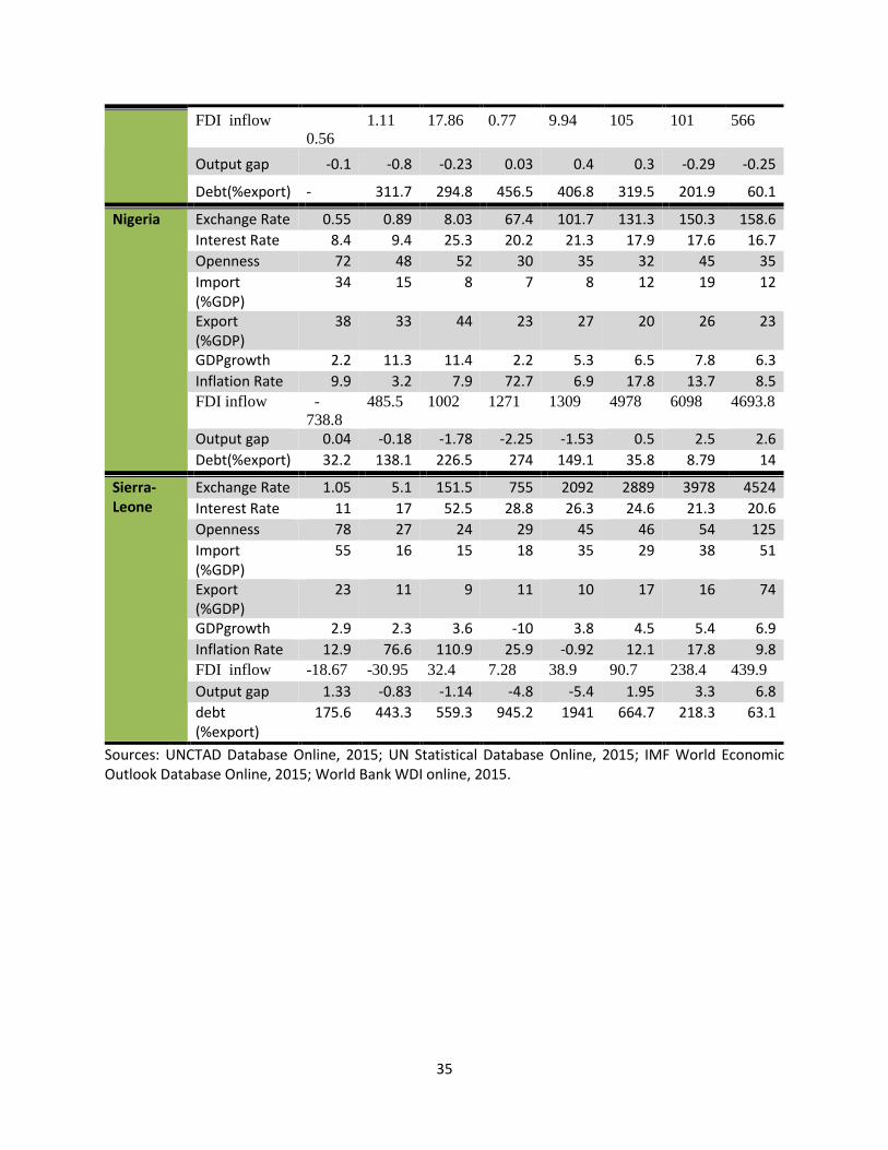
35

FDI inflow

0.56

1.11 17.86 0.77 9.94 105 101 566

Output gap -0.1 -0.8 -0.23 0.03 0.4 0.3 -0.29 -0.25

Debt(%export) - 311.7 294.8 456.5 406.8 319.5 201.9 60.1

Nigeria Exchange Rate 0.55 0.89 8.03 67.4 101.7 131.3 150.3 158.6

Interest Rate 8.4 9.4 25.3 20.2 21.3 17.9 17.6 16.7

Openness 72 48 52 30 35 32 45 35

Import (%GDP)

34 15 8 7 8 12 19 12

Export (%GDP)

38 33 44 23 27 20 26 23

GDPgrowth 2.2 11.3 11.4 2.2 5.3 6.5 7.8 6.3

Inflation Rate 9.9 3.2 7.9 72.7 6.9 17.8 13.7 8.5

FDI inflow -

738.8

485.5 1002 1271 1309 4978 6098 4693.8

Output gap 0.04 -0.18 -1.78 -2.25 -1.53 0.5 2.5 2.6

Debt(%export) 32.2 138.1 226.5 274 149.1 35.8 8.79 14

Sierra-Leone

Exchange Rate 1.05 5.1 151.5 755 2092 2889 3978 4524

Interest Rate 11 17 52.5 28.8 26.3 24.6 21.3 20.6

Openness 78 27 24 29 45 46 54 125

Import (%GDP)

55 16 15 18 35 29 38 51

Export (%GDP)

23 11 9 11 10 17 16 74

GDPgrowth 2.9 2.3 3.6 -10 3.8 4.5 5.4 6.9

Inflation Rate 12.9 76.6 110.9 25.9 -0.92 12.1 17.8 9.8

FDI inflow -18.67 -30.95 32.4 7.28 38.9 90.7 238.4 439.9

Output gap 1.33 -0.83 -1.14 -4.8 -5.4 1.95 3.3 6.8

debt (%export)

175.6 443.3 559.3 945.2 1941 664.7 218.3 63.1

Sources: UNCTAD Database Online, 2015; UN Statistical Database Online, 2015; IMF World Economic Outlook Database Online, 2015; World Bank WDI online, 2015.

36

Recent Publications in the Series

nº Year Author(s) Title

247 2017 Adamon N. Mukasa, Anthony M.

Simpasa, Adeleke O. Salami

Credit constraints and farm productivity: Micro-level

evidence from smallholder farmers in Ethiopia

246 2017 Abebe Shimeles and Tiguene

Nabassaga Why is inequality high in Africa?

245 2016 Anthony Simpasa and Lauréline Pla Sectoral Credit Concentration and Bank Performance in

Zambia

244 2016 Ellen B. McCullough Occupational Choice and Agricultural Labor Exits in

Sub-Saharan Africa

243 2016 Brian Dillon Selling crops early to pay for school: A large-scale

natural experiment in Malawi

242 2016 Edirisa Nseera

Understanding the Prospective Local Content in the

Petroleum Sector and the Potential Impact of High

Energy Prices on Production Sectors and Household

Welfare in Uganda

241 2016 Paul Christian and Brian Dillon Long term consequences of consumption seasonality

240 2016 Kifle Wondemu and David Potts

The Impact of the Real Exchange Rate Changes on

Export Performance in Tanzania and Ethiopia

239 2016 Audrey Verdier-Chouchane and

Charlotte Karagueuzian

Concept and Measure of Inclusive Health across

Countries

238 2016

Sébastien Desbureaux, Eric

Nazindigouba Kéré and Pascale

Combes Motel

Impact Evaluation in a Landscape: Protected Natural

Forests, Anthropized Forested Lands and Deforestation

Leakages in Madagascar’s Rainforests

37