arX

iv:0

809.

4122

v2 [

astr

o-ph

] 1

Dec

200

8

Mon. Not. R. Astron. Soc. 000, 1–14 (2008) Printed 16 November 2018 (MN LATEX style file v2.2)

Perturbation theory of N point-mass gravitational lens

systems without symmetry: small mass-ratio

approximation

H. AsadaFaculty of Science and Technology, Hirosaki University, Hirosaki 036-8561, Japan

Accepted Received

ABSTRACTThis paper makes the first systematic attempt to determine using perturbation theorythe positions of images by gravitational lensing due to arbitrary number of coplanarmasses without any symmetry on a plane, as a function of lens and source parameters.We present a method of Taylor-series expansion to solve the lens equation under a smallmass-ratio approximation. First, we investigate perturbative structures of a single-complex-variable polynomial, which has been commonly used. Perturbative roots arefound. Some roots represent positions of lensed images, while the others are unphysicalbecause they do not satisfy the lens equation. This is consistent with a fact that thedegree of the polynomial, namely the number of zeros, exceeds the maximum numberof lensed images if N=3 (or more). The theorem never tells which roots are physical (orunphysical). In this paper, unphysical ones are identified. Secondly, to avoid unphysicalroots, we re-examine the lens equation. The advantage of our method is that it allowsa systematic iterative analysis. We determine image positions for binary lens systemsup to the third order in mass ratios and for arbitrary N point masses up to the secondorder. This clarifies the dependence on parameters. Thirdly, the number of the imagesthat admit a small mass-ratio limit is less than the maximum number. It is suggestedthat positions of extra images could not be expressed as Maclaurin series in massratios. Magnifications are finally discussed.

Key words: gravitational lensing – cosmology: theory – stars: general – methods:analytical.

1 INTRODUCTION

Gravitational lensing has become one of important subjectsin modern astronomy and cosmology (e.g., Schneider 2006,Weinberg 2008). It has many applications as gravitationaltelescopes in various fields ranging from extra-solar planetsto dark matter and dark energy at cosmological scales. Thispaper focuses on gravitational lensing due to a N-point masssystem. Indeed it is a challenging problem to express theimage positions as functions of lens and source parameters.There are several motivations. One is that gravitational lens-ing offers a tool of discoveries and measurements of plane-tary systems (Schneider and Weiss 1986, Mao and Paczynski1991, Gould and Loeb 1992, Bond et al. 2004, Beaulieu et al.2006), compact stars, or a cluster of dark objects, which aredifficult to probe with other methods. Gaudi et al. (2008)have recently found an analogy of the Sun-Jupiter-Saturnsystem by lensing. Another motivation is theoretically ori-ented. One may be tempted to pursue a transit between aparticle method and a fluid (mean field) one. For microlens-

ing studies, particle methods are employed, because the sys-tems consist of stars, planets or MACHOs. In cosmologicallensing, on the other hand, light propagation is consideredfor the gravitational field produced by inhomogeneities ofcosmic fluids, say galaxies or large scale structures of theuniverse (e.g., Refregier 2003 for a review). It seems natu-ral, though no explicit proof has been given, that observedquantities computed by continuum fluid methods will agreewith those by discrete particle ones in the limit N → ∞, atleast on average, where N is the number of particles.

Related with the problems mentioned above, we shouldnote an astronomically important effect caused by the finite-ness of N . For most of cosmological gravitational lenses(both of strong and weak ones), a continuum approxima-tion can be safe and has worked well. There exists an excep-tional case, however, for which discreteness becomes impor-tant. One example is a quasar microlensing due to a point-like lens object, which is possibly a star in a host galaxy(for an extensive review, Wambsganss 2006). A galaxy con-sists of very large number N particles, and light rays from

c© 2008 RAS

2 H. Asada

an object at cosmological distance may have a chance topass very near one of the point masses. As a consequence offinite-N effect in large N point lenses, anomalous changes inthe light curve are observed. For such a quasar microlensing,hybrid approaches are usually employed, where particles arelocated in a smooth gravitational field representing a hostgalaxy. It is thus likely that N point-mass approach will beuseful also when we study such a finite-N effect at a certaintransit stage between a particles system and a smooth one.Along this course, An (2007) investigated a N point lensmodel, which represents a very special configuration thatevery point masses are located on regular grid points.

For a N point-mass lens at a general configuration, veryfew things are known in spite of many efforts. Among knownones is the maximum number of images lensed by N pointmasses. After direct calculations by Witt (1990) and Mao,Petters and Witt (1997), a careful study by Rhie (2001 forN=4, 2003 for general N) revealed that it is possible to ob-tain the maximum number of images as 5(N − 1). This the-orem for polynomials has been extended to a more generalcase including rational functions by Khavinson and Neu-mann (2006). (See Khavinson and Neumann 2008 for an el-egant review on a connection between the gravitational lenstheory and the algebra, especially the fundamental theoremof algebra, and its extension to rational functions).

Theorem (Khavinson and Neumann 2006):Let r(z) = p(z)/q(z), where p and q are relatively primepolynomials in z, and let n be the degree of r. If n > 1,then the number of zeros for r(z) − z∗ ≤ 5(n − 1). Here, zand z∗ denote a complex number and its complex conjugate,respectively.

Furthermore, Bayer, Dyer and Giang (2006) showedthat in a configuration of point masses, replacing one of thepoint deflectors by a spherically symmetric distributed massonly introduces one extra image. Hence they found that themaximum number of images due to N distributed lensingobjects located on a plane is 6(N − 1) + 1.

Global properties such as lower bounds on the numberof images are also discussed in Petters, Levine and Wambs-ganss (2001) and references therein.

In spite of many efforts on N lensing objects, functionsfor image positions are still unknown even for N point-masslenses in a general configuration under the thin lens approx-imation. Hence it is a challenging problem to express theimage positions as functions of lens and source locations.Once such an expression is known, one can immediately ob-tain magnifications via computing the Jacobian of the lensmapping (Schneider et al. 1992).

Only for a very few cases such as a single point massand a singular isothermal ellipsoid, the lens equation can besolved by hand and image positions are known, because thelens equation becomes a quadratic or fourth-order one (Fora singular isothermal ellipsoid, Asada et al. 2003). For thebinary lens system, the lens equation has the degree of fivein a complex variable (Witt 1990). It has the same degreealso in a real variable (Asada 2002a, Asada et al. 2004). Thisimprovement is not trivial because a complex variable bringstwo degrees of freedom. This single-real-variable polynomialhas advantages. For instance, the number of real roots (withvanishing imaginary parts) corresponds to that of lensed im-ages. The analytic expression of the caustic, where the num-ber of images changes, is obtained by the fifth-order poly-

nomial (Asada et al. 2002c). Galois showed, however, thatthe fifth-order and higher polynomials cannot be solved al-gebraically (van der Waerden 1966). Hence, no formula forthe quintic equation is known. For this reason, some numer-ical implementation is required to find out image positions(and magnifications) for the binary gravitational lens for ageneral position of the source. Only for special cases of thesource at a symmetric location such as on-axis sources, thelens equation can be solved by hand and image positionsare thus known (Schneider and Weiss 1986). For a weakfield region, some perturbative solutions for the binary lenshave been found (Bozza 1999, Asada 2002b), for instancein order to discuss astrometric lensing, which is caused bythe image centroid shifts (for a single mass, Miyamoto andYoshii 1995, Walker 1995; for a binary lens, Safizadeh et al.1999, Jeong et al. 1999, Asada 2002b).

If the number of point masses N is larger than two, thebasic equation is much more highly non-linear so that thelens equation can be solved only by numerical methods. Asa result, observational properties such as magnifications andimage separations have been investigated so far numericallyfor N point-mass lenses. This makes it difficult to investigatethe dependence of observational quantities on lens parame-ters.

This paper is the first attempt to seek an analytic ex-pression of image positions without assuming any specialsymmetry. For this purpose, we shall present a method ofTaylor-series expansion to solve the lens equation for Npoint-mass lens systems. Our method allows a systematiciterative analysis as shown later.

Under three assumptions of weak gravitational fields,thin lenses and small deflection angles, gravitational lensingis usually described as a mapping from the lens plane ontothe source plane (Schneider et al. 1992). Bourassa and Kan-towski (1973, 1975) introduced a complex notation to de-scribe gravitational lensing. Their notation was exclusivelyused to describe lenses with elliptical or spheroidal symme-try (Borgeest 1983, Bray 1984, Schramm 1990). For N pointlenses, Witt (1990) succeeded in recasting the lens equationinto a single-complex-variable polynomial. This is in an el-egant form and thus has been often used in investigationsof point-mass lenses. An advantage in the single-complex-variable formulation is that we can use some mathemati-cal tools applicable to complex-analytic functions, especiallypolynomials (Witt 1993, Witt and Petters 1993, Witt andMao 1995). One tool is the fundamental theorem of algebra:Every non-constant single-variable polynomial with complexcoefficients has at least one complex root. This is also statedas: every non-zero single-variable polynomial, with complexcoefficients, has exactly as many complex roots as its degree,if each root is counted as many times as its multiplicity. Onthe other hand, in the original form of the lens equation, onecan hardly count up the number of images because of non-linearly coupled properties. This theorem, therefore, raisesa problem in gravitational lensing. The single-variable poly-nomial due to N point lenses has the degree of N2 + 1,though the maximum number of images is 5(N − 1). Thismeans that unphysical roots are included in the polynomial(for detailed discussions on the disappearance and appear-ance of images near fold and cusp caustics for general lenssystems, see also Petters, Levine and Wambsganss (2001)and references therein). First, we thus investigate explicitly

c© 2008 RAS, MNRAS 000, 1–14

Gravitational Lensing by N Point Mass 3

behaviors of roots for the polynomial lens equation fromthe viewpoint of perturbations. We shall identify unphysicalroots. Secondly, we shall re-examine the lens equation, sothat the appearance of unphysical roots can be avoided.

This paper is organised as follows. In Section 2, thecomplex description of gravitational lensing is briefly sum-marised. The lens equation is embedded into a single-complex-variable polynomial in Section 3. Perturbativeroots for the complex polynomial are presented for binaryand triple systems in sections 4 and 5, respectively. They areextended to a case of N point lenses in section 6. In section 7,we re-examine the lens equation in a dual-complex-variablesformalism and its perturbation scheme for a binary lens forits simplicity. The perturbation scheme is extended to a Npoint lens system in section 8. Section 9 is devoted to theconclusion.

2 POLYNOMIAL FORMALISM USINGCOMPLEX VARIABLES

We consider a lens system with N point masses. The massand two-dimensional location of each body is denoted as Mi

and the vector Ei, respectively. For the later convenience,let us define the angular size of the Einstein ring as

θE =

√

4GMtotDLSc2DLDS

, (1)

where G is the gravitational constant, c is the light speed,Mtot is the total mass

∑N

i=1Mi and DL, DS and DLS de-

note distances between the observer and the lens, betweenthe observer and the source, and between the lens and thesource, respectively. In the unit normalised by the angularsize of the Einstein ring, the lens equation becomes

β = θ −

N∑

i

νiθ − ei

|θ − ei|2, (2)

where β = (βx, βy) and θ = (θx, θy) denote the vectors forthe position of the source and image, respectively and wedefined the mass ratio and the angular separation vector asνi = Mi/Mtot and ei = Ei/θE = (eix, eiy).

In a formalism based on complex variables, two-dimensional vectors for the source, lens and image positionsare denoted as w = βx+iβy , z = θx+iθy, and ǫi = eix+ieiy,respectively (See also Fig. 1). By employing this formalism,the lens equation is rewritten as

w = z −

N∑

i

νiz∗ − ǫ∗i

, (3)

where the asterisk ∗ means the complex conjugate. The lensequation is non-analytic because it contains both z and z∗.

3 EMBEDDING THE LENS EQUATION INTOAN ANALYTIC POLYNOMIAL

The complex conjugate of Eq. (3) is expressed as

w∗ = z∗ −

N∑

i

νiz − ǫi

. (4)

Figure 1. Notation: The source and image positions on complexplanes are denoted by w (the circle) and z (the filled disk), re-spectively. Locations of N point masses are denoted by ǫi (filledtriangles) for i = 1, · · · , N . Here, we assume the thin lens approx-imation.

This expression can be substituted into z∗ in Eq. (3) toeliminate the complex variable z∗. As a result, we obtaina (N2 + 1)-th order analytic polynomial equation as (Witt1990)

(z −w)

N∏

ℓ=1

(

(w∗ − ǫ∗ℓ )

N∏

k=1

(z − ǫk) +

N∑

k=1

νk

N∏

j 6=k

(z − ǫj)

)

=

N∑

i=1

νi

N∏

ℓ=1

(z − ǫℓ)

×

N∏

m6=i

(

(w∗ − ǫ∗m)

N∏

k=1

(z − ǫk) +

N∑

k=1

νk

N∏

j 6=k

(z − ǫj)

)

.

(5)

Equation (A3) in Witt (1990) takes a rather complicatedform because of inclusion of nonzero shear γ due to sur-rounding matter. Bayer et al. (2006) uses a complex formal-ism in order to discuss the maximum number of images in aconfiguration of point masses, by replacing one of point de-flectors by a spherically symmetric distributed mass. Theirlens equation (3) agrees with Eq. (5). In order to show thisagreement, one may use (−1)N+1 = (−1)N−1. It is worth-while to mention that Eq. (5) contains not only all the solu-tions for the lens equation (2) but also unphysical false rootswhich do not satisfy Eq. (2), in price of the manipulationfor obtaining an analytic polynomial equation, as alreadypointed out by Rhie (2001, 2003) and Bayer et al. (2006).Such an inclusion of unphysical solutions can be easily un-derstood by remembering that we get unphysical roots aswell as true ones if one takes a square of an equation includ-ing the square root. In fact, an analogous thing happens inanother example of gravitational lenses such as an isother-mal ellipsoidal lens as a simple model of galaxies (Asada etal. 2003).

In general, the mass ratio νi satisfies 0 < νi < 1, so thatit can be taken as an expansion parameter. Without loss ofgenerality, we can assume that the first lens object is the

c© 2008 RAS, MNRAS 000, 1–14

4 H. Asada

most massive, namely m1 ≥ mi for i = 2, 3, · · · , N . Thus,formal solutions are expressed in Taylor series as

z =

∞∑

p2=0

∞∑

p3=0

· · ·

∞∑

pN=0

νp22 νp3

3 · · · νpNN z(p2)(p3)···(pN ), (6)

where the coefficients z(p2)(p3)···(pN ) are independent of νi.Up to this point, the origin of the lens plane is arbitrary.

In the following, the origin of the lens plane is chosen as thelocation of the mass m1, such that one can put ǫ1 = 0.This enables us to simplify some expressions and to easilyunderstand their physical meanings, mostly because gravityis dominated by m1 in most regions except for the vicinityof mi (i 6= 1). Namely, it is natural to treat our problemas perturbations around a single lens by m1 (located at theorigin of the coordinates).

In numerical simulations or practical data analysis,however, one may use the coordinates in which the origin isnot the location of m1. If one wishes to consider such a caseof ǫ1 6= 0, one could make a translation by ǫ1 as z → z+ ǫ1,w → w + ǫ1 and ǫi → ǫi + ǫ1 in our perturbative solutionsthat are given below.

4 PERTURBATIVE SOLUTIONS FOR APOLYNOMIAL FORMALISM 1: BINARYLENS

In this section, we investigate binary lenses explicitly up tothe third order. This simple example may help us to un-derstand the structure of the perturbative solutions. For anarbitrary N case, expressions of iterative solutions are quiteformal (See below).

For simplicity, we denote our expansion parameter asm ≡ ν2. This means ν1 = 1 −m. We also denote ǫ2 simplyby ǫ.

In powers of m, the polynomial equation is rewritten as

2∑

k=0

mkfk(z) = 0, (7)

where we defined

f0(z) = (z − ǫ)2[(w∗ − ǫ∗)z + 1](w∗z2 −ww∗z − w),

f1(z) = (z − w)

×(

ǫ(z −w)[(2w∗ − ǫ∗)z + 2]− ǫ∗z2(z − ǫ)− ǫz)

,

f2(z) = ǫ2(z − w). (8)

We seek a solution in expansion series as

z =

∞∑

p=0

mpz(p). (9)

4.1 0th order

At O(m0), the lens equation becomes the fifth-order polyno-mial equation as f0 = 0. Zeroth order solutions are obtainedby solving this. All the solutions are ǫ (doublet), α3 and α±,where we defined

α3 =1

ǫ∗ − w∗,

α± =w

2

(

1±

√

1 +4

ww∗

)

. (10)

One of the roots, α3, is unphysical, because it does not sat-isfy Eq. (2) at O(m0). By using all the 0th order roots in-cluding unphysical ones, f0 is factorised as

f0(z) = w∗(w∗ − ǫ∗)(z − ǫ)2(z − α3)(z − α+)(z − α−). (11)

4.2 1st order

Next, we seek 1st-order roots. We put z = α± + mz(1) +O(m2). At the linear order in m, Eq. (5) becomes

z(1)f′

0(α±) + f1(α±) = 0, (12)

where the prime denotes the derivative with respect to z.Thereby we obtain a 1st-order root as

z(1) = −f1(α±)

f′

0(α±). (13)

The similar manner cannot be applied to a case of ǫ, becauseit is a doublet root with f0(ǫ) = f

′

0(ǫ) = 0, while f′′

0 (ǫ) 6= 0.At O(m2), Eq. (5) can be factorised as

(

z(1)[(w∗ − ǫ∗)ǫ+ 1] + ǫ

)

×(

z(1)[(ǫ− w)(w∗ǫ+ 1)− ǫ] + ǫ(ǫ− w))

= 0. (14)

Hence, we obtain two roots as

z(1) =ǫ

(ǫ∗ − w∗)ǫ− 1, (15)

z(1) = −ǫ(ǫ −w)

(ǫ− w)(w∗ǫ+ 1)− ǫ. (16)

Here, the latter root expressed by Eq. (16) is unphysical andthus abandoned, because it doesn’t satisfy the original lensequation (2). On the other hand, the former root by Eq. (15)satisfies the equation and thus expresses a physically correctimage.

4.3 2nd Order

First, we consider perturbations around zeroth-order solu-tions of α±. At O(m2), Eq. (5) is linear in z(2) and thuseasily solved for z(2) as

z(2) = −z2(1)f

′′

0 (α±) + 2z(1)f′

1(α±) + 2f2(α±)

2f′

0(α±). (17)

Next, we investigate a multiple root ǫ. At O(m3), Eq.(5) becomes linear in z(2). It is solved as

z(2) = −z3(1)f

′′′

0 (ǫ) + 3z2(1)f′′

1 (ǫ) + 6z(1)f′

2(ǫ)

6[z(1)f′′

0 (ǫ) + f′

1(ǫ)]. (18)

4.4 3rd Order

Around zeroth-order solutions of α±, Eq. (5) at O(m3) islinear in z(2) and thus solved as

z(3) = −1

f′

0(α±)[z(1)z(2)f

′′

0 (α±) +1

6z3(1)f

′′′

0 (α±)

+z(2)f′

1(α±) +1

2z2(1)f

′′

1 (α±) + z(1)f′

2(α±)]. (19)

c© 2008 RAS, MNRAS 000, 1–14

Gravitational Lensing by N Point Mass 5

Also around the multiple root ǫ, Eq. (5) at O(m3) be-comes linear in z(2). It is solved as

z(3) = −1

z(1)f′′

0 (ǫ) + f′

1(ǫ)

×[1

2z2(2)f

′′

0 (ǫ) +1

2z2(1)z(2)f

′′′

0 (ǫ) +1

24z4(1)f

′′′′

0 (ǫ)

+z(1)z(2)f′′

1 (ǫ) +1

6z3(1)f

′′′

1 (ǫ)

+2z(2)f′

2(ǫ)], (20)

where we used f′′

2 (z) = 0.Table 1 shows a numerical example of perturbative roots

and their convergence.

5 PERTURBATIVE SOLUTIONS FOR APOLYNOMIAL FORMALISM 2: TRIPLETLENS

In a binary case, we have only the single parameter m forthe perturbations. For N point masses, we have to take ac-count of couplings among several expansion parameters. Inaddition, the degree of the polynomial becomes N2 + 1, sothat we cannot write down the whole equation. In order toget hints for N point-mass lenses, in this section, we inves-tigate triple-mass lenses explicitly up to the second order inν2 and ν3.

The polynomial equation is rewritten as

3∑

p2=0

3∑

p3=0

(ν2)p2(ν3)

p3g(p2)(p3)(z) = 0, (21)

where we defined

g(0)(0)(z) = (z − ǫ2)3(z − ǫ3)

3[(w∗ − ǫ∗2)z + 1]

×[(w∗ − ǫ∗3)z + 1](w∗z2 − ww∗z −w). (22)

We seek a solution in expansion series as

z =

∞∑

p2=0

∞∑

p3=0

(ν2)p2(ν3)

p3z(p2)(p3). (23)

5.1 0th order

Zeroth order solutions are obtained by solving the tenth-order polynomial equation as g(0)(0) = 0. The roots are ǫ2(doublet), ǫ3 (doublet), α3, α4 and α±, where we defined

α3 =1

ǫ∗2 −w∗,

α4 =1

ǫ∗3 −w∗. (24)

For the same reason in the binary lens, α3 and α4 are un-physical, in the sense that it does not satisfy the lens equa-tion (2). By using all the 0th order roots, g(0)(0) is factorisedas

g(0)(0)(z) = w∗(w∗ − ǫ∗2)(w∗ − ǫ∗3)(z − ǫ2)

3(z − ǫ3)3

×(z − α3)(z − α4)(z − α+)(z − α−). (25)

5.2 1st order

Here, we seek 1st-order roots. The image position is ex-panded as z = α±+ν2z(1)(0)+ν3z(0)(1)+O(ν2

2 , ν23 , ν2ν3). By

making a replacement in notations as 2 ↔ 3, one can con-struct z(0)(1) from z(1)(0). Hence, we focus on z(1)(0) below.At the linear order in ν2, Eq. (5) becomes

z(1)(0)g′

(0)(0)(α±) + g(1)(0)(α±) = 0. (26)

Thereby we obtain a 1st-order root as

z(1)(0) = −g(1)(0)(α±)

g′

(0)(0)(α±)

. (27)

For the triple mass lens system, the root ǫ2 becomestriplet with g(00)(ǫ2) = g

′

(00)(ǫ2) = g′′

(00)(ǫ2) = 0, while

g′′′

(00)(ǫ) 6= 0. After rather lengthy but straightforward calcu-

lations, Eq. (5) at O(ν22 ) can be factorised as

(

z(1)(0)[(w∗ − ǫ∗2)ǫ2 + 1] + ǫ2

)

×(

z(1)(0)[(w∗ − ǫ∗3)ǫ2 + 1] + ǫ2

)

×(

z(1)(0)[(ǫ2 − w)(w∗ǫ2 + 1)− ǫ2] + ǫ2(ǫ2 −w))

= 0. (28)

Hence, we obtain three roots as

z(1)(0) =ǫ2

(ǫ∗2 − w∗)ǫ2 − 1, (29)

z(1)(0) =ǫ2

(ǫ∗3 − w∗)ǫ2 − 1, (30)

z(1)(0) = −ǫ2(ǫ2 − w)

(ǫ2 − w)(w∗ǫ2 + 1)− ǫ2. (31)

At the linear order in ν2, true solutions for the triple lenssystem has to agree with that for the binary system, whenone takes a limit as ν3 → 0. Therefore, out of the abovethree roots, ones expressed by Eqs. (30) and (31) must beabandoned.

6 PERTURBATIVE SOLUTIONS FOR APOLYNOMIAL FORMALISM 3: NPOINT-MASS LENS

In the previous section, we have learned couplings betweenthe second and third masses. Now we are in a position toinvestigate a lens system consisting of N point masses.

The polynomial lens equation (5) is expanded as

N∑

p2=0

N∑

p3=0

· · ·

N∑

pN=0

(ν2)p2(ν3)

p3 · · · (νN)pN

×g(p2)(p3)···(pN )(z) = 0. (32)

For this equation, we seek a solution in expansion series as

z =

∞∑

p2=0

∞∑

p3=0

· · ·

∞∑

pN=0

(ν2)p2(ν3)

p3 · · · (νN )pN

×z(p2)(p3)···(pN ). (33)

6.1 0th order

Zeroth order solutions are obtained by solving the (N2 +1)th-order polynomial equation as g(0)···(0) = 0. The roots

c© 2008 RAS, MNRAS 000, 1–14

6 H. Asada

Table 1. Example of perturbative roots in the single-complex-polynomial: We assume ν = 0.1, e = 1 and two cases of w = 2 (on-axis)and w = 1 + i (off-axis). In this example, the number of images is three. ”Polynomial” in the table means all the five roots for thesingle-complex-polynomial. They are obtained by numerically solving the polynomial. Image positions are determined also by numericallysolving the lens equation. They are listed in the column ”Lens Eq.”. In the table, ”None” means that it does not exist. These tables showthat, as we go to higher orders, the perturbative roots become closer to the correct ones for the single-complex-polynomial, including the

two unphysical roots.

Case 1 On-axis ν = 0.1 e = 1 w = 2

Root 1 2 3 4 5

1st. 2.43921 -0.389214 0.95 -0.925 0.9752nd. 2.43855 -0.388551 0.95 -0.924063 0.9740633rd. 2.43858 -0.388519 0.949938 -0.924016 0.974016

Polynomial 2.43858 -0.388517 0.949937 -0.924013 0.974013

Lens Eq. 2.43858 -0.388517 0.949937 None None

Case 2 Off-axis ν = 0.1 e = 1 w = 1 + i

Root 1 2 3 4 5

1st. 1.33716+1.40546 i -0.337158-0.355459 i 0.95-0.05 i 0.025-0.925 i 0.975-0.025 i2nd. 1.33632+1.40363 i -0.336316-0.354881 i 0.95-0.05 i 0.02625-0.9225 i 0.97375-0.02625 i3rd. 1.33634+1.40371 i -0.336275-0.354839 i 0.95-0.05025 i 0.0262813-0.922281 i 0.973656-0.0263438 i

Polynomial 1.33633+1.40371 i -0.336272-0.354835 i 0.950015-0.0502659 i 0.0262762-0.922254 i 0.973646-0.0263517 i

Lens Eq. 1.33633+1.40371 i -0.336272-0.354835 i 0.950015-0.0502659 i None None

are αi ≡ −1/w∗i , α±, and ǫi (with multiplicity = N) for

i = 2, · · ·N , where for later convenience we denoted

wi = w − ǫi. (34)

Like in the binary lens, αi is unphysical, in the sense that itdoes not satisfy the lens equation (2). By using all the 0thorder roots, g(0)···(0) is factorised as

g(0)···(0)(z) = (z − α+)(z − α−)w∗

N∏

j=2

(w∗j )

×

N∏

k=2

(z − ǫk)N

N∏

ℓ=2

(z +1

w∗ℓ

), (35)

where this degree is N2 + 1 in agreement with that of thepolynomial equation.

6.2 1st order

Next, we seek 1st-order roots. In the similar manner in thedouble or triple mass case, we can obtain a 1st-order root as

z(0)···(1k)···(0) = −g(0)···(1k)···(0)(α±)

g′

(0)···(0)(α±)

, (36)

where 1k denotes that the k-th index is the unity, namelypk = 1.

For N point mass lens systems, a root ǫk is multipletwith multiplicity = N . Without loss of generality, we chooseǫ2 as a root in the following discussion. Calculations doneabove for a double or triple mass system suggest that Eq.

(5) at O(ν22 ) can be factorised as

N∏

k=2

(

z(1)(0)···(0)[(w∗k)ǫ2 + 1] + ǫ2

)

×(

z(1)(0)···(0)[w2(w∗ǫ2 + 1) + ǫ2] + ǫ2w2

)

= 0. (37)

By using this factorisation, we obtain N roots. At the linearorder in ν2, however, true solutions for the present lens sys-tem has to agree with that for the binary system, becauseone can take the limit as νp → 0 for p ≥ 3. Therefore, onlythe −ǫ2/(w

∗2ǫ2 + 1) out of the above N roots is correct for

the original lens equation. The same argument is true of anyǫi.

7 PERTURBATIVE SOLUTIONS FORZZ∗-DUAL FORMALISM 1: BINARY LENS

As shown above, an analytic polynomial formalism is appar-ently simple. When we solve perturbatively the polynomialequation, however, we find unphysical roots which satisfy thepolynomial but does not the original lens equation. In thepolynomial formalism, therefore, we are required to checkevery roots and then to pick up only the physical roots sat-isfying the original lens equation with discarding unphysicalones. It is even worse that the order of the polynomial growsrapidly asN2+1, as the number of the lens objects increases.This means that the perturbative structure of the formalismbecomes much more complicated as N increases. In this sec-tion, we thus investigate another formalism, which allows amore straightforward calculation especially without needingextra procedures such as deleting physically incorrect roots.

c© 2008 RAS, MNRAS 000, 1–14

Gravitational Lensing by N Point Mass 7

First, we focus on a binary case for its simplicity. Thelens equation is rewritten as

C(z, z∗) = mD(z∗), (38)

where we defined

C(z, z∗) = w − z +1

z∗, (39)

D(z∗) =1

z∗−

1

z∗ − ǫ∗. (40)

One of advantages in this zz∗-formulation is that themaster equation (38) is linear in m. Therefore, counting or-ders in m can be drastically simplified when we performiterative calculations. On the other hand, an analytic poly-nomial is second order in m. In fact, practical perturbativecomputations in the polynomial formalism are quite compli-cated, in the sense that several different terms (f0, f1 and f2for a binary case) may make the same order-of-magnitudecontributions at each iteration step.

We seek a solution in expansion series as

z =

∞∑

k=0

mkz(k). (41)

The complex conjugate of this becomes

z∗ =

∞∑

k=0

mkz∗(k). (42)

According to these power-series expansions of z and z∗, bothsides of the lens equation are expanded as

C(z, z∗) =

∞∑

k=0

mkC(k), (43)

D(z∗) =

∞∑

k=0

mkD(k), (44)

where C(k) and D(k) are independent of m. At O(mk), Eq.(38) becomes

C(k) = D(k−1), (45)

which shows clearly a much simpler structure than a polyno-mial case such as Eqs. (17) and (18). Equation (40) indicatesthat D(z∗) has a pole at z∗ = ǫ∗. Therefore, we shall discusstwo cases of z(0) 6= ǫ and z(0) = ǫ, separately.

7.1 0th order (z(0) 6= ǫ)

Zeroth order solutions are obtained by solving the equationas

C(z(0), z∗(0)) = 0. (46)

The solution for this is the well-known roots for a singlemass lens. In order to help readers to understand the zz∗-dual formulation, we shall derive the roots by keeping bothz and z∗. In conventional treatments, a single lens case isreduced to one-dimensional one by choosing the source di-rection along the x-axis in vector formulations or the realaxis in complex ones. Eq. (46) is rewritten as

z(0)z∗(0) − 1 = wz∗(0). (47)

The L. H. S. is purely real so that the R. H. S. must bereal. Unless w = 0, therefore, one can put z(0) = Aw byintroducing a certain real number A. By substituting z(0) =Aw into Eq. (47), one obtains a quadratic equation for A as

ww∗A2 − ww∗A− 1 = 0. (48)

This is solved as

A =1

2

(

1±

√

1 +4

ww∗

)

, (49)

which gives the 0th-order solution.In the special case of w = 0, Eq. (47) becomes |z(0)| =

1, which is the Einstein ring. In the following, we assumew 6= 0.

7.2 1st order (z(0) 6= ǫ)

In units of z(0), the expansion series of z is normalised as

z = z(0)

∞∑

k=0

mkσ(k), (50)

where we defined σ(k) = z(k)/z(0).First, we investigate a case of z(0) 6= ǫ. At the linear

order in m, Eq. (38) becomes

z(1) +z∗(1)

(z∗(0)

)2= −

1

z∗(0)

+1

z∗(0)

− ǫ∗. (51)

In order to solve Eq. (51), we consider an equation linearin both z and z∗ as

z + az∗ = b, (52)

for two complex constants a, b ∈ C.Unless |a| = 1, the general root for this equation is

z =b− ab∗

1− aa∗. (53)

This can be verified by a direct substitution of Eq. (53) intoEq. (52). If |a| = 1, Eq. (52) is underdetermined, in thesense that it could not provide the unique root without anyadditional constraint condition on z and z∗.

By using directly Eq. (53), Eq. (51) is solved as

z(1) =1

z2(0)

(z∗(0)

)2 − 1

(

ǫ∗z2(0)z∗(0)

z∗(0)

− ǫ∗−

ǫz(0)z(0) − ǫ

)

. (54)

7.3 2nd order (z(0) 6= ǫ)

At O(m2), Eq. (38) is

z(2) + a2z∗(2) = b2, (55)

where we defined

a2 =1

(z∗(0))2, (56)

b2 = −D(1) +(σ∗

(1))2

z∗(0)

. (57)

Here, D(1) is written as

D(1) = −σ∗(1)

z∗(0)

+σ∗(1)

z∗(0)

− ǫ∗. (58)

c© 2008 RAS, MNRAS 000, 1–14

8 H. Asada

By using the relation (53), Eq. (55) is solved as

z(2) =b2 − a2b

∗2

1− a2a∗2

. (59)

7.4 3rd order and nth order (z(0) 6= ǫ)

Computations at O(m3) are similar to those at O(m2) asshown below. At O(m3), Eq. (38) takes a form as

z(3) + a3z∗(3) = b3, (60)

where we defined

a3 =1

(z∗(0)

)2, (61)

b3 = −D(2) +2σ∗

(1)σ∗(2) − (σ∗

(1))3

z∗(0)

. (62)

Here, D(2) is written as

D(2) = −σ∗(2) − (σ∗

(1))2

z∗(0)+

z∗(2)

(z∗(0) − ǫ∗)2−

(z∗(1))2

(z∗(0) − ǫ∗)3. (63)

Using the relation (53) for Eq. (60), we obtain

z(3) =b3 − a3b

∗3

1− a3a∗3

. (64)

In the similar manner, one can obtain iteratively nth-order roots z(n), which obeys an equation in the form of Eq.(52), and thus can use Eq. (53) to obtain z(n).

7.5 0th and 1st order (z(0) = ǫ)

Next, we investigate the vicinity of z = ǫ, which is a pole ofD. The other pole of D is z = 0, which makes also C(z, z∗)divergent. Therefore, z = 0 and its neighbourhood are aban-doned. Let us focus on a root around z = ǫ.

We assume z = ǫ +mz(1) +O(m2). Then, the relevantterms in expansion series of C and D become

C(0) = w − ǫ +1

ǫ∗, (65)

D(−1) = −1

z∗(1)

, (66)

where the index −1 means that the inverse of m appears be-cause of the pole at ǫ. Therefore, the lens equation at O(m0)becomes linear in z∗(1) without including z(1). Immediately,it determines z∗(1). Its complex conjugate becomes

z(1) = −ǫ

(w∗ − ǫ∗)ǫ+ 1. (67)

This shows a clear difference between z(0) = ǫ and z(0) 6= ǫcases. Equation (51) for the latter case contains both z(1)and z∗(1), so that we must use a relation such as Eq. (53).

7.6 2nd, 3rd and nth order (z(0) = ǫ)

Next, we consider the lens equation at O(m1), namelyC(1) = D(0). This determines z∗(2) as

z∗(2) = (z∗(1))2(

C(1) −1

ǫ∗

)

, (68)

where we may use

-1 0 1 2 3-2

-1

0

1

2

xy

Figure 2. Perturbative image positions for a binary lens case.This plot corresponds to Tables 1 and 2. The lenses (e1 = 0, e2 =1) and sources (w = 2 and w = 1+i) are denoted by filled squares.The image positions are denoted by filled disks. Perturbative im-ages at the 1st, 2nd and 3rd orders are overlapped so that wecannot distinguish them in this figure.

C(1) = −z(1) −z∗(1)

(ǫ∗)2. (69)

Let us consider O(m2) to look for z(3). Equation ofC(2) = D(1) provides z∗(3) as

z∗(3) = (z∗(1))2C(2) +

(z∗(1))3

(ǫ∗)2+

(z∗(2))2

z∗(1)

, (70)

where we can use

C(2) = −z(2) −z∗(2)

(ǫ∗)2+

(z∗(1))2

(ǫ∗)3. (71)

By the same way, one can obtain perturbatively nth-ordersolutions z(n) around z(0) = ǫ.

Table 2 shows an example of perturbative roots inthe dual-complex-variables formalism and their convergence.Tables 1 and 2 suggest that the polynomial approach and thedual-complex-variables formalism are consistent with eachother, regarding the true images. Figure 2 shows image po-sitions on the lens plane, corresponding to these tables.

8 PERTURBATIVE SOLUTIONS FORZZ∗-DUAL FORMALISM 2: LENSING BY NPOINT MASS

The purpose of this section is to extend the proposed methodto a general case of gravitational lensing by an arbitrarynumber of point masses.

The lens equation is written as

C(z, z∗) =

N∑

k=2

νkDk(z∗), (72)

c© 2008 RAS, MNRAS 000, 1–14

Gravitational Lensing by N Point Mass 9

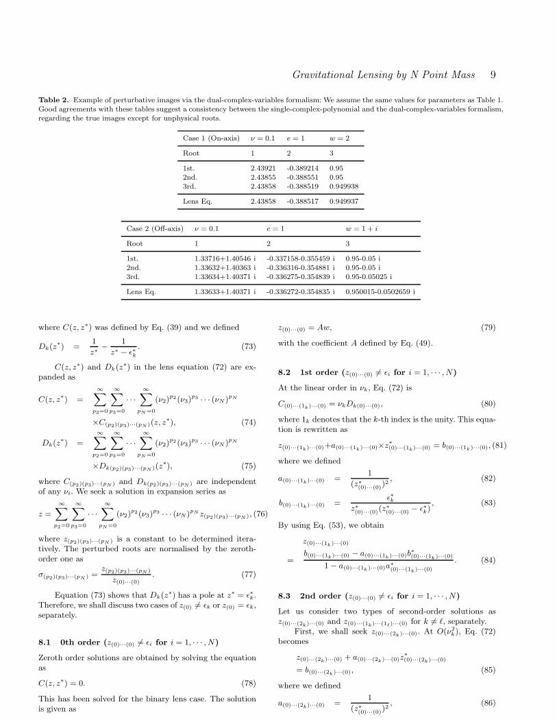
Table 2. Example of perturbative images via the dual-complex-variables formalism: We assume the same values for parameters as Table 1.Good agreements with these tables suggest a consistency between the single-complex-polynomial and the dual-complex-variables formalism,regarding the true images except for unphysical roots.

Case 1 (On-axis) ν = 0.1 e = 1 w = 2

Root 1 2 3

1st. 2.43921 -0.389214 0.952nd. 2.43855 -0.388551 0.953rd. 2.43858 -0.388519 0.949938

Lens Eq. 2.43858 -0.388517 0.949937

Case 2 (Off-axis) ν = 0.1 e = 1 w = 1 + i

Root 1 2 3

1st. 1.33716+1.40546 i -0.337158-0.355459 i 0.95-0.05 i2nd. 1.33632+1.40363 i -0.336316-0.354881 i 0.95-0.05 i3rd. 1.33634+1.40371 i -0.336275-0.354839 i 0.95-0.05025 i

Lens Eq. 1.33633+1.40371 i -0.336272-0.354835 i 0.950015-0.0502659 i

where C(z, z∗) was defined by Eq. (39) and we defined

Dk(z∗) =

1

z∗−

1

z∗ − ǫ∗k. (73)

C(z, z∗) and Dk(z∗) in the lens equation (72) are ex-

panded as

C(z, z∗) =

∞∑

p2=0

∞∑

p3=0

· · ·

∞∑

pN=0

(ν2)p2(ν3)

p3 · · · (νN )pN

×C(p2)(p3)···(pN )(z, z∗), (74)

Dk(z∗) =

∞∑

p2=0

∞∑

p3=0

· · ·

∞∑

pN=0

(ν2)p2(ν3)

p3 · · · (νN )pN

×Dk(p2)(p3)···(pN )(z∗), (75)

where C(p2)(p3)···(pN ) and Dk(p2)(p3)···(pN ) are independentof any νi. We seek a solution in expansion series as

z =

∞∑

p2=0

∞∑

p3=0

· · ·

∞∑

pN=0

(ν2)p2(ν3)

p3 · · · (νN )pN z(p2)(p3)···(pN ), (76)

where z(p2)(p3)···(pN ) is a constant to be determined itera-tively. The perturbed roots are normalised by the zeroth-order one as

σ(p2)(p3)···(pN ) =z(p2)(p3)···(pN )

z(0)···(0). (77)

Equation (73) shows that Dk(z∗) has a pole at z∗ = ǫ∗k.

Therefore, we shall discuss two cases of z(0) 6= ǫk or z(0) = ǫk,separately.

8.1 0th order (z(0)···(0) 6= ǫi for i = 1, · · · , N)

Zeroth order solutions are obtained by solving the equationas

C(z, z∗) = 0. (78)

This has been solved for the binary lens case. The solutionis given as

z(0)···(0) = Aw, (79)

with the coefficient A defined by Eq. (49).

8.2 1st order (z(0)···(0) 6= ǫi for i = 1, · · · , N)

At the linear order in νk, Eq. (72) is

C(0)···(1k)···(0) = νkDk(0)···(0), (80)

where 1k denotes that the k-th index is the unity. This equa-tion is rewritten as

z(0)···(1k)···(0)+a(0)···(1k)···(0)×z∗(0)···(1k)···(0) = b(0)···(1k)···(0), (81)

where we defined

a(0)···(1k)···(0) =1

(z∗(0)···(0)

)2, (82)

b(0)···(1k)···(0) =ǫ∗k

z∗(0)···(0)

(z∗(0)···(0)

− ǫ∗k), (83)

By using Eq. (53), we obtain

z(0)···(1k)···(0)

=b(0)···(1k)···(0) − a(0)···(1k)···(0)b

∗(0)···(1k)···(0)

1− a(0)···(1k)···(0)a∗(0)···(1k)···(0)

. (84)

8.3 2nd order (z(0)···(0) 6= ǫi for i = 1, · · · , N)

Let us consider two types of second-order solutions asz(0)···(2k)···(0) and z(0)···(1k)···(1ℓ)···(0) for k 6= ℓ, separately.

First, we shall seek z(0)···(2k)···(0). At O(ν2k), Eq. (72)

becomes

z(0)···(2k)···(0) + a(0)···(2k)···(0)z∗(0)···(2k)···(0)

= b(0)···(2k)···(0), (85)

where we defined

a(0)···(2k)···(0) =1

(z∗(0)···(0)

)2, (86)

c© 2008 RAS, MNRAS 000, 1–14

10 H. Asada

b(0)···(2k)···(0) = −Dk(0)···(1k)···(0) +(σ∗

(0)···(1k)···(0))2

z∗(0)···(0)

,(87)

where Dk(0)···(1k)···(0) is written as

Dk(0)···(1k)···(0) = −z∗(0)···(1k)···(0)(

1

(z∗(0)···(0)

)2−

1

(z∗(0)···(0)

− ǫk)2

)

.(88)

By using the relation (53) for Eq. (85), we obtain

z(0)···(2k)···(0)

=b(0)···(2k)···(0) − a(0)···(2k)···(0)b

∗(0)···(2k)···(0)

1− a(0)···(2k)···(0)a∗(0)···(2k)···(0)

. (89)

Next, let us determine z(0)···(1k)···(1ℓ)···(0). At O(νkνℓ)for k < ℓ, Eq. (72) becomes

z(0)···(1k)···(1ℓ)···(0)

+a(0)···(1k)···(1ℓ)···(0)z∗(0)···(1k)···(1ℓ)···(0)

= b(0)···(1k)···(1ℓ)···(0), (90)

where we defined

a(0)···(1k)···(1ℓ)···(0) =1

(z∗(0)···(0)

)2, (91)

b(0)···(1k)···(1ℓ)···(0) = −Dk(0)···(1ℓ)···(0) −Dℓ(0)···(1k)···(0)

+2σ∗

(0)···(1k)···(0)σ∗(0)···(1ℓ)···(0)

z∗(0)···(0)

. (92)

Here, Dk(0)···(1ℓ)···(0) and Dℓ(0)···(1k)···(0) are written as

Dk(0)···(1ℓ)···(0)

= −z∗(0)···(1ℓ)···(0)

(

1

(z∗(0)···(0)

)2−

1

(z∗(0)···(0)

− ǫk)2

)

,(93)

Dℓ(0)···(1k)···(0)

= −z∗(0)···(1k)···(0)

(

1

(z∗(0)···(0)

)2−

1

(z∗(0)···(0)

− ǫℓ)2

)

.(94)

By using the relation (53) for Eq. (90), we obtain

z(0)···(1k)···(1ℓ)···(0)

=b(0)···(1k)···(1ℓ)···(0) − a(0)···(1k)···(1ℓ)···(0)b

∗(0)···(1k)···(1ℓ)···(0)

1− a(0)···(1k)···(1ℓ)···(0)a∗(0)···(1k)···(1ℓ)···(0)

.

(95)

8.4 0th and 1st order (z(0)···(0) = ǫk)

Next, we investigate the vicinity of z = ǫk, which is a poleof Dk. The other pole of Dk is z = 0, which makes C(z, z∗)divergent. Therefore, z = 0 and its neighbourhood are aban-doned. Let us focus on a root around

z(0)···(0) = ǫk. (96)

If we admitted z(0)···(1ℓ)···(0) around ǫk for l 6= k, onlythe Dk function would contain the inverse of νℓ, whichintroduces a term at O(νk/νℓ) in the lens equation andleads to inconsistency. Namely, the lens equation prohibitsz(0)···(1ℓ)···(0) around ǫk for l 6= k. This agrees with the poly-nomial case. We thus assume z = ǫk + νkz(0)···(1k)···(0) +O(ν2

k). Then, we obtain

C(0)···(0) = w − ǫk +1

ǫ∗k, (97)

D(0)···(−1k)···(0) = −1

z∗(0)···(1k)···(0)

, (98)

where −1k means that the inverse of νk appears because ofthe pole at ǫk. Therefore, the lens equation at O(ν0

k) becomeslinear in z∗(0)···(1k)···(0) without including z(0)···(1k)···(0). Im-mediately, it determines z∗(0)···(1k)···(0). Hence, its complexconjugate provides

z(0)···(1k)···(0) = −ǫk

(w∗ − ǫ∗k)ǫk + 1. (99)

8.5 2nd order (z(0)···(0) = ǫk)

Here, we consider the lens equation at O(ν1k), namely

C(0)···(1k)···(0) = D(0)···(0), where

D(0)···(0) =1

ǫ∗k+

z∗(0)···(2k)···(0)

(z∗(0)···(1k)···(0)

)2. (100)

Hence, we obtain z∗(0)···(2k)···(0) and thereby its complex con-jugate as

z(0)···(2k)···(0) = (z(0)···(1k)···(0))2

(

C∗(0)···(1k)···(0) −

1

ǫ∗k

)

, (101)

where C(0)···(1k)···(0) becomes

C(0)···(1k)···(0) = −

(

z(0)···(1k)···(0) +z∗(0)···(1k)···(0)

ǫ∗2k

)

. (102)

Next, we consider a root at O(ν1kν

1ℓ ), where we can as-

sume k < ℓ without loss of generality. At this order, theinverse of νk appears. The lens equation at O(ν1

ℓ ) becomes

C(0)···(1ℓ)···(0) = Dk(0)···(−1k)···(0) +Dℓ(0)···(0), (103)

where

Dk(0)···(−1k)···(1ℓ)···(0) =z∗(0)···(1k)···(1ℓ)···(0)

(z∗(0)···(1k)···(0)

)2. (104)

Hence, we obtain z∗(0)···(1k)···(1ℓ)···0)and thereby its com-

plex conjugate as

z(0)···(1k)···(1ℓ)···(0)

= (z(0)···(1k)···(0))2

×(

C∗(0)···(1ℓ)···(0)

−D∗ℓ(0)···(0)

)

, (105)

where C(0)···(1ℓ)···(0) and Dℓ(0)···(0) are written as

C(0)···(1ℓ)···(0) = −z(0)···(1ℓ)···(0) −z∗(0)···(1ℓ)···(0)

ǫ∗2k

, (106)

Dℓ(0)···(0) =1

ǫ∗k−

1

ǫ∗k − ǫ∗ℓ. (107)

This direct computation shows that z(0)···(1k)···(1ℓ)···(0) doesnot exist because z(0)···(1ℓ)···(0) is prohibited in the vicinityof ǫk. This is also consistent with the polynomial case at thesecond order.

8.6 Magnifications

Before closing this paper, it is worthwhile to mention mag-nifications by N point-mass lensing in the framework of thepresent perturbation theory that is intended to solve thelens equation to obtain image positions. The amplification

c© 2008 RAS, MNRAS 000, 1–14

Gravitational Lensing by N Point Mass 11

-2 -1 0 1 21.00

1.05

1.10

1.15

1.20

1.25

t

A

-2 -1 0 1 2-0.0004

-0.0002

0.0000

0.0002

0.0004

t

∆A

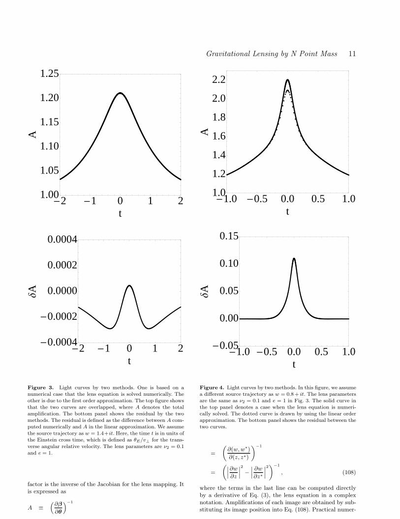
Figure 3. Light curves by two methods. One is based on anumerical case that the lens equation is solved numerically. Theother is due to the first order approximation. The top figure showsthat the two curves are overlapped, where A denotes the totalamplification. The bottom panel shows the residual by the twomethods. The residual is defined as the difference between A com-puted numerically and A in the linear approximation. We assumethe source trajectory as w = 1.4+it. Here, the time t is in units ofthe Einstein cross time, which is defined as θE/v⊥ for the trans-

verse angular relative velocity. The lens parameters are ν2 = 0.1and e = 1.

factor is the inverse of the Jacobian for the lens mapping. Itis expressed as

A ≡(

∂β

∂θ

)−1

-1.0 -0.5 0.0 0.5 1.01.0

1.2

1.4

1.6

1.8

2.0

2.2

tA

-1.0 -0.5 0.0 0.5 1.0-0.05

0.00

0.05

0.10

0.15

t

∆A

Figure 4. Light curves by two methods. In this figure, we assumea different source trajectory as w = 0.8+ it. The lens parametersare the same as ν2 = 0.1 and e = 1 in Fig. 3. The solid curve inthe top panel denotes a case when the lens equation is numeri-cally solved. The dotted curve is drawn by using the linear orderapproximation. The bottom panel shows the residual between thetwo curves.

=

(

∂(w,w∗)

∂(z, z∗)

)−1

=

(

∣

∣

∣

∂w

∂z

∣

∣

∣

2

−∣

∣

∣

∂w

∂z∗

∣

∣

∣

2)−1

, (108)

where the terms in the last line can be computed directlyby a derivative of Eq. (3), the lens equation in a complexnotation. Amplifications of each image are obtained by sub-stituting its image position into Eq. (108). Practical numer-

c© 2008 RAS, MNRAS 000, 1–14

12 H. Asada

Figure 5. Graph representations of interactions among pointmasses for images at the second order level. The top and bot-tom graphs represent a mutually-interacting image and a self-interacting one, respectively.

ical estimations may follow this procedure. For illustratingthis, Figs. 3 and 4 show examples of light curves by a binarylens via the perturbative approach. These curves are wellreproduced. However, double peaks due to caustic crossingscannot be reproduced by the present method.

As an approach enabling a simpler argument before go-ing to numerical estimations, we use the functional formof perturbed image positions. In the perturbation theory,lensed images can be split into two groups. One is thattheir zeroth-order root is not located at a lens object(z(0)···(0) 6= ǫk). In the other group, zeroth-order roots orig-inate from a lens position at ǫk. We call the former andlatter ones mutually-interacting and self-interacting images,respectively, because all the lens objects make contributionsto mutually-interacting images at the linear order as shownby Eq. (84). On the other hand, self-interacting images areinfluenced only by the nearest lens object at ǫk at the lin-ear and even at the second orders as shown by Eqs. (99)and (101). Figure 5 shows graph representations for the twogroups of images.

For the simplicity, we consider stretching of imagesroughly as |∂z/∂w|, though rigorously speaking it must bethe amplification. Table 1 and Equation (76) mean that thecomplex derivative becomes for mutually-interacting images

∂z

∂w=

∂z(0)···(0)∂w

+∑

k

νk∂z(0)···(1k)···(0)

∂w, (109)

and for self-interacting images

∂z

∂w= νk

∂z(0)···(1k)···(0)∂w

, (110)

where we used that ǫk is a constant.For the simplicity, we assume νk = O(1/N) for a large N

case. Then, the linear order term in self-interacting images isO(1/N), and thus they become negligible as N → ∞. On theother hand, mutually-interacting ones have non-vanishingterms even at the zeroth order. Hence, they can play a cru-cial role.

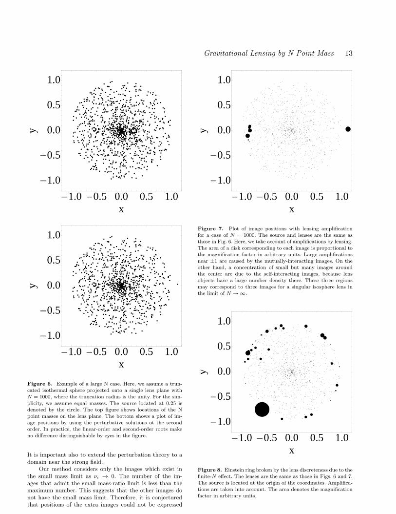
However, we should take account of a spatial distribu-tion of lens objects. If they are clustering and thus denseat a certain region, then the total flux of light throughsuch a dense region is not negligible any more. Let us de-note the fraction of the clustering particles by f . Totalcontributions from such clustering self-interacting imagesare estimated approximately as a typical image magnifi-cation multiplied by the number of the particles, namelyfN × νk(∼ 1/N) = O(f), which does not vanish even asN → ∞. Figures 6 and 7 show an example of a large Ncase, where N is chosen as 1000.

9 CONCLUSION

Under a small mass-ratio approximation, this paper devel-oped a perturbation theory of N coplanar (in the thin lensapproximation) point-mass gravitational lens systems with-out symmetries on a plane. The system can be separatedinto a single mass lens as a background and its perturbationdue to the remaining point masses.

First, we investigated perturbative structures of thesingle-complex-variable polynomial, into which the lensequation is embedded. Some of zeroth-order roots of thepolynomial do not satisfy the lens equation and thus areunphysical. This appearance of correct but unphysical rootsis consistent with the earlier work on a theorem on the max-imum number of lensed images (Rhie 2001, 2003). However,the theorem never tells which roots are physical (or unphys-ical). What we did is that unphysical roots are identified.

Next, we re-examined the lens equation in the dual-complex-variables formalism to avoid inclusions of unphysi-cal roots. We presented an explicit form of perturbed imagepositions as a function of source and lens positions. As akey tool for perturbative computations, Eq. (53) was alsofound. For readers’ convenience, the perturbative roots arelisted in Table 3. If one wishes to go to higher orders, ourmethod will enable one to easily use computer algebra soft-wares such as MAPLE and MATHEMATICA. This is be-cause it requires simpler algebra (only the four basic opera-tions of arithmetic), compared with vector forms which needextra operations such as inner and outer products.

There are numerous possible applications along thecourse of the perturbation theory of N point-mass gravi-tational lens systems. For instance, it will be interesting tostudy lensing properties such as magnifications by using thefunctional form of image positions. Furthermore, the validityof the present result may be limited in the weak field regions.

c© 2008 RAS, MNRAS 000, 1–14

Gravitational Lensing by N Point Mass 13

-1.0 -0.5 0.0 0.5 1.0

-1.0

-0.5

0.0

0.5

1.0

x

y

-1.0 -0.5 0.0 0.5 1.0

-1.0

-0.5

0.0

0.5

1.0

x

y

Figure 6. Example of a large N case. Here, we assume a trun-cated isothermal sphere projected onto a single lens plane withN = 1000, where the truncation radius is the unity. For the sim-plicity, we assume equal masses. The source located at 0.25 isdenoted by the circle. The top figure shows locations of the Npoint masses on the lens plane. The bottom shows a plot of im-age positions by using the perturbative solutions at the secondorder. In practice, the linear-order and second-order roots makeno difference distinguishable by eyes in the figure.

It is important also to extend the perturbation theory to adomain near the strong field.

Our method considers only the images which exist inthe small mass limit as νi → 0. The number of the im-ages that admit the small mass-ratio limit is less than themaximum number. This suggests that the other images donot have the small mass limit. Therefore, it is conjecturedthat positions of the extra images could not be expressed

-1.0 -0.5 0.0 0.5 1.0

-1.0

-0.5

0.0

0.5

1.0

xy

Figure 7. Plot of image positions with lensing amplificationfor a case of N = 1000. The source and lenses are the same asthose in Fig. 6. Here, we take account of amplifications by lensing.The area of a disk corresponding to each image is proportional tothe magnification factor in arbitrary units. Large amplificationsnear ±1 are caused by the mutually-interacting images. On theother hand, a concentration of small but many images aroundthe center are due to the self-interacting images, because lensobjects have a large number density there. These three regionsmay correspond to three images for a singular isosphere lens inthe limit of N → ∞.

-1.0 -0.5 0.0 0.5 1.0

-1.0

-0.5

0.0

0.5

1.0

x

y

Figure 8. Einstein ring broken by the lens discreteness due to thefinite-N effect. The lenses are the same as those in Figs. 6 and 7.The source is located at the origin of the coordinates. Amplifica-tions are taken into account. The area denotes the magnificationfactor in arbitrary units.

c© 2008 RAS, MNRAS 000, 1–14

14 H. Asada

Table 3. List of the coefficients in perturbative positions of im-ages lensed by N point masses: The image positions are expressedin the form of z =

∑

p2· · ·∑

pN(ν2)p2 · · · (νN )pN z(p2)···(pN ).

The top and bottom panels show the cases of z(0)···(0) = ǫi andz(0)···(0) 6= ǫi, respectively. In the columns, ”None” means thatthe corresponding coefficient does not exist.

Case 1: z(0)···(0) 6= ǫi (i = 1, · · · , N)

z(0)···(0) Eq. (79)

z(0)···(1k)···(0) Eqs. (82)-(84)

z(0)···(2k)···(0) Eqs. (86)-(89)

z(0)···(1k)···(1ℓ)···(0) Eqs. (91)-(95)

Case 2: z(0)···(0) = ǫk

z(0)···(0) Eq. (96)

z(0)···(1k)···(0) Eqs. (99)

z(0)···(1ℓ)···(0) for ℓ 6= k None

z(0)···(2k)···(0) Eq. (101)

z(0)···(1k)···(1ℓ)···(0)for ℓ 6= k None

as Maclaurin series in mass ratios. This may be implied alsoby previous works. For instance, the appearance of the max-imum number of images for a binary lens requires a finitemass ratio and the caustic crossing (Schneider and Weiss1986). Regarding this point, further studies will be neededto determine positions of all the images with the maximumnumber as a function of lens and source parameters.

ACKNOWLEDGMENTS

The author would like to thank S. Mao, N. Rattenbury andE. Kerins for the hospitality at the Manchester Microlens-ing Conference, where this work was initiated. He is gratefulalso to D. Bennett and Y. Muraki for stimulating conversa-tions at the conference. He wishes to thank F. Abe, J. Bayerand D. Khavinson for useful comments on the manuscript.This work was supported in part by a Japanese Grant-in-Aid for Scientific Research from the Ministry of Education,No. 19035002.

REFERENCES

An J. H., 2007, MNRAS, 376, 1814Asada H., 2002a, A&A, 390, L11Asada H., 2002b, ApJ, 573, 825Asada H., Kasai T., Kasai M., 2002c, Prog. Theor. Phys.,108, 1031Asada H., Hamana T., Kasai M., 2003, A&A, 397, 825Asada H., Kasai T., Kasai M., 2004, Prog. Theor. Phys.,112, 241Bayer J., Dyer C. C., Giang D., 2006, Gen. Rel. Grav., 38,1379Beaulieu J. P., et al., 2006, Nature, 439, 437Bond I. A., et al., 2004, ApJ, 606, L155Borgeest U., 1983, A&A, 128, 162

Bourassa R. R., Kantowski R., Norton T. D., 1973, ApJ,185, 747Bourassa R. R., Kantowski R., 1975, ApJ, 195, 13Bozza V., 1999, A&A, 348, 311Bray I., 1984, MNRAS, 208, 511Gaudi B. S., et al., 2008, Science, 319, 927Gould A., Loeb A., 1992, ApJ, 396, 104Jeong Y., Han C., Park S., 1999, ApJ, 511, 569Khavinson D., Neumann G., 2006, Proc. Amer. Math. Soc.134, 1077Khavinson D., Neumann G., 2008, Not. Amer. Math. Soc.55, 666Mao S., Paczynski B., 1991, ApJ, 374, 37LMao S., Petters A., Witt H. J., 1997, in Proceedings

of the Eighth Marcel Grossmann Meeting on General

Relativity, Ed. R. Ruffini, (Singapore, World Scientific)astro-ph/9708111Miyamoto M., Yoshii Y., 1995, AJ, 110, 1427Petters A. O., Levine H., Wambsganss J., 2001, Singularitytheory and gravitational lensing (Boston, Birkhauser)Refregier A., 2003, ARAA, 41, 645Rhie S. H., 2001, arXiv:astro-ph/0103463Rhie S. H., 2003, arXiv:astro-ph/0305166Safizadeh N., Dalal N., Griest K., 1999, ApJ, 522, 512Schneider P., Weiss A., 1986, A&A. 164, 237Schneider P., Ehlers J., Falco E. E., 1992, Gravitational

Lenses (Heidelberg, Springer-Verlag)Schneider P., 2006, Extragalactic Astronomy And Cosmol-

ogy: An Introduction (Heidelberg, Springer-Verlag)Schramm T., 1990, A&A, 231, 19van der Waerden B. L., 1966, Algebra I (Heidelberg,Springer-Verlag)Walker M. A., 1995, ApJ, 453, 37Wambsganss J., 2006, in Proceedings of the 33rd Saas-

Fee Advanced Course (Heidelberg, Springer-Verlag): arXiv:astro-ph/0604278Weinberg S., 2008, Cosmology (Oxford, Oxford Univ.Press)Witt H. J., 1990, A&A. 236, 311Witt H. J., 1993, ApJ, 403, 530Witt H. J., Petters A., 1993, J. Math. Phys. 34, 4093Witt H. J., Mao S., 1995, ApJ. 447, L105

This paper has been typeset from a TEX/ LATEX file preparedby the author.

c© 2008 RAS, MNRAS 000, 1–14