FACTOR-PRICE CHANGES, PROFIT, and LONG-RUN EQUILIBRIUM

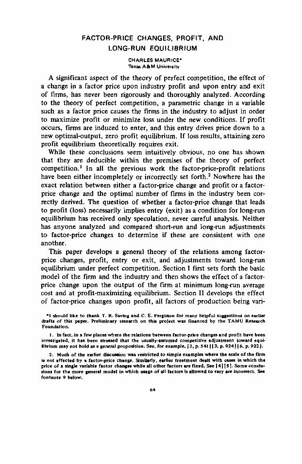
FACTOR-PRICE CHANGES, PROFIT, AND LONG-RUN EQU I LI BR I UM

CHARLES MAURICE. Texas A & M University

A significant aspect of the theory of perfect competition, the effect of a change in a factor price upon industry profit and upon entry and exit of firms, has never been rigorously and thoroughly analyzed. According to the theory of perfect competition, a parametric change in a variable such as a factor price causes the firms in the industry to adjust in order to maximize profit or minimize loss under the new conditions. If profit occurs, f i s are induced to enter, and this entry drives price down to a new optimal-output, zero profit equilibrium. If loss results, attaining zero profit equilibrium theoretically requires exit.

While these conclusions seem intuitively obvious, no one has shown that they are deducible within the premises of the theory of perfect competition.' In all the previous work the factor-price-profit relations have been either incompletely or incorrectly set forth? Nowhere has the exact relation between either a factor-price change and profit or a factor- price change and the optimal number of f m s in the industry been correctly derived. The question of whether a factor-price change that leads to profit (loss) necessarily implies entry (exit) as a condition for long-run equilibrium has received only speculation, never careful analysis. Neither has anyone analyzed and compared short-run and long-run adjustments to factor-price changes to determine if these are consistent with one another. This paper develops a general theory of the relations among factor-

price changes, profit, entry or exit, and adjustments toward long-run equilibrium under perfect competition. Section I first sets forth the basic model of the f i and the industry and then shows the effect of a factor- price change upon the output of the firm at minimum long-run average cost and at profit-maximizing equilibrium. Section I1 develops the effect of factor-price changes upon profit, all factors of production being vari-

*I should like to thank T. R. Saving and C. E. Ferguson for many helpful suggestions on earti- drafts of this paper. Retiminary research on this project was financed by the TAMU Research Foundation.

1. In fact, in a few places where the relations between factor-price changes and profit have been investigated, it har been stressed that the usually-auumed competitive adjustment toward equilibrium may not hold as a general proposition. See, for example, 12, p. 541 1 [ 3, p. 924) [ 6, p. 922).

2. Much of the earlier discmaion was rertricted to simple examples where the scale of the firm is not affected by a factor-price change. Similarly. earlier treatment dealt with case8 in which the price of a single variable factor chsnga while all other factors are fixed. See 141 [ 51. Some conclusions for the more general model in which usage of all factors is allowed to vary are inconect. See footnote 9 below.

64

MAURICE: LONG-RUN EQUILIBRIUM 65

able but the number of firms remaining futed. The results depend in large part on the effect of the price change upon the optimal output of the fm. Section I11 derives the relation between a factor-price change and the change in the optimal number of firms. It is then shown that if all factors are variable, conditions causing profit (loss) must cause the optimal number of f m s to increase (decrease). That is, in the long run, profit or loss is always a correct signal. Finally, short-run adjustments when some inputs are fixed are compared with long-run adjustments when all inputs are variable.

1. BASIC MODEL

The concern of this paper is upon the way in which a factor-price change affects the profit of firms in the industry and the optimal number of firms. These responses depend upon the effect of the factor-price change upon the firm’s output under two differing conditions: (1 ) the output is forced to conform to long-run competitive equilibrium; (2) the output is forced to conform to equilibrium in the commodity market, while the number of f m s is held constant and each fm is in profit- maximizing, but not long-run competitive, equilibrium. These two output responses are analyzed in this section. The analysis begins with the standard textbook model of the perfectly competitive fm and industry in long-run equilibrium. Let the prices of all factors be parametrically given to the industry, and, for simplicity, let all f m s be identical. The f m in long-run equilibrium is described as follows:

The production and cost functions are

(1) q = f (XI. xz, . . . , x,) n

i= I c = c pixi

where q is rate of physical output, c is cost, and xi and pi are the rate of physical input and the price of the i-th factor. Efficiency requires the marginal product of each factor to equal its price divided by marginal cost. Thus

(3) fi - xpi = 0 ( i = l , 2, ..., n)

where l /X = marginal cost. The second order conditions are that

(4) (i . j = l , 2, ..., nl

be associated with a negative definite quadratic form. For profit maximi-

66 WESTERN ECONOMIC JOURNAL

zation marginal cost must equal commodity price, and for competitive equilibrium marginal cost must equal average cost:

(5 1 where p is commodity price. Finally, second order conditions for profit maximization require that

(6 ) iF*l= i4,I (i, j = l , 2, ..., n)

be associated with a negative definite quadratic form.

relations:

Commodity price must satisfy the demand function

p = 1/x = c/q

Equilibrium in the commodity market is defined by the following

where QD is quantity demanded. Market clearing requires quantity demanded to equal quantity supplied:

N is the number of f m s , assumed, for simplicity, to be continuously dif- ferentiable, and q is, as above, the output of the typical firm. In long-run competitive equilibrium QD is the quantity demanded at the price that equals minimum long-run average cost, q is optimal output, and N is the optimal number of firms.

Equations ( 1 ) - (8) set forth the standard model of the perfectly competitive firm in long-run equilibrium. Three additional definitions are necessary to what follows. The responsiveness of output, firm size, profit, and the number of firms to a factor-price change will be described throughout this paper in terms of three elasticities. The first, q D , is the demand elasticity for the commodity. Second, the elasticity of marginal cost, qMC, is the relative responsiveness of marginal cost to changes in output, the adjustment taking place along the long-run marginal cost curve. Third, the expenditure elasticity of the j-th factor, q,, is the relative responsiveness of the usage of the j-th factor to a change in cost, the adjustment taking place along the expansion path. In other words, it is the ratio of the proportional change in the usage of the j-th factor to the proportional change in expenditure on all factors taken together. These three elasticities are defined in terms of the demand function and the Hessian and bordered Hessian determinants of the production function:

Demand elasticity is


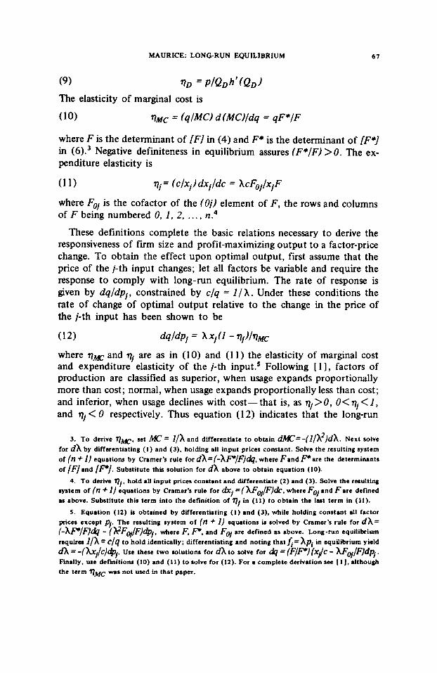
where F is the determinant of IF1 in (4) and F* is the determinant of IF*] in (6).3 Negative definiteness in equilibrium assures (F*/F) >0. The expenditure elasticity is

(1 1) qj= ( C / X ~ ) dXj/dC = XCFoj/XjF

where Foj is the cofactor of the (0j) element of F, the rows and columns of F being numbered 0. 1, 2, .... n.

These definitions complete the basic relations necessary to derive the responsiveness of firm size and profit-maximizing output to a factor-price change. To obtain the effect upon optimal output, first assume that the price of the j-th input changes; let all factors be variable and require the response to comply with long-run equilibrium. The rate of response is given by dq/dpj, constrained by c/q = I / X . Under these conditions the rate of change of optimal output relative to the change in the price of the j-th input has been shown to be

4

(12) dqldpj = X X j ( 1 - qj)/qm

where qM and qj are as in (10) and (1 1 ) the elasticity of marginal cost and expenditure elasticity of the j-th input.’ Following [ 1 I , factors of production are classified as superior, when usage expands proportionally more than cost; normal, when usage expands proportionally less than cost; and inferior, when usage declines with cost- that is, as qj > 0, 0< qj < 1, and qj<O respectively. Thus equation (12) indicates that the long-run

3. To derive qm. set = I/h and differentiate t o obtain W = - ( 1 / X 2 ) d X . Next solve for dX by differentiating ( 1 ) and (3), holding all input prices constant. Solve the resulting system of (?I + 1) equations by Cramer’s rule for dh=(-hP,F))dq, where F a n d P a r e the determinants of [F land [PI. Substitute this solution for dX above to obtain equation (10).

4. To derive Q j , h d d all input prices constant and differentiate (2) and (3). Solve the resulting system of (n + 1) equations by Cramer’s rule for = ( U w / F ) & , where Fo, and F a r e defined as above. Substitute this term into the definition of q, in (11) t o obtain the last term in (11).

5. Equation (12) is obtained by differentiating (1) and (3), while holding constant all factor prices except pj. The resulting system of (n + 1) equations is solved by Crnmer’s rule for dX= (-wffl& - (h?F@/F)@j. where F. P, and Fq are defined as above. Long-fun equilibrium requires ]/A= C / q to hold identically; differentiating and noting tha t f i=Xpi in equilibrium yield dx = -(hrf/c)@j. Use these two solutions for dx to solve for & = ( F / P ) ( X ~ C - AFq/F)dpj. Finally, use defmitionr (10) and (11) to solve for (12). For a complete derivation see [ 11, although the term qMc w a s not used in that paper.


equilibrium output of the firm varies directly with the price of a normal or inferior factor and inversely with the price of a normal factor.6

To derive the second form of dq/dpi, the profit-maximizing response, assume, once again, an industry in long-run equilibrium. This time let the price of the j-th input change while holding the number of firms in the industry constant. The factor-price change shifts the marginal cost curves and, therefore, shifts industry supply. Product price moves along commodity demand as f i s attempt to maximize profit. Let the existing firms attain profit-maximizing, but not long-run competitive, equilibrium, and require the commodity market to be in equilibrium; that is p = l/X = h(QD). Under these assumptions it can be shown that the rate of response of the typical f i ’ s output is7

(1 3) dq/dPi = qqj q D x i / ( ] - 7)D qm)

where q D , q j , and qw are as defined in (9), ( lo) , and (! 1). Since r)D is negative, the sign of (13) is positive for an inferior factor and negative Itherwise. This result is to be expected because, as shown in [ 11, marginal :ost falls after an increase in the price of an inferior factor and rises after m increase in the price of a normal or superior factor. When the number of firms is held constant, industry output varies directly with the sign of (13).

To summarize, equations (12) and (13) indicate the rates of response of the typical firm’s optimal output and profit-maximizing output (the number of f m s held constant) to a change in the price of the j-th factor. It is now possible to investigate profit, entry, and exit.

11. FACTOR-PRICE CHANGES AND PROFIT

The first relation to be investigated is the way in which the profit of each firm changes after the price of an input changes. Allow sufficient time for a!! factors to be variable, but insufficient time for firms to enter or exit in response to the profit or loss signal and drive profit to zero. Let the typical firm’s profit (1 ) be given by

6. If qj = 1, average cost shifts directly upward, the minimum point occurring at the same quantity as before. If ‘7, = 0, average cost shifts along a stationary marginal cost curve. See [ 1 1 for a more complete discussion and graphical analysis.

7. To derive equation (13) begin as in footnote 5 by differentiating ( 1 ) and (3). then solving the resulting system of (n + 1) equation1 for d A = -( AP/F)J&I - (%?Fw/F)dp/. where the notation is the same as above. Since profit maximization requires commodity price to equal marginal cost d p = -(l/??)dX. Equilibrium in the commodity market requires that dp = h’(QD)dQ =N(+/aq)dq. Using these three equations, mhe for dq/dpj; substitute definitions (9). (10). and (11) and evaluate in oridnal equilibrium where l / X = C/q. Since the number of firms is constant, equation (9 ) is now = p / ( ap/%)Nq.

MAURICE: L O N G R U N EQUILIBRIUM 69

To establish the relation between factor-price changes and profit of f m s in the industry, the sign of dn/dpi must be determined, holding the number of firms constant but letting the usage of all inputs vary. To this end, begin in long-run equilibrium with n = 0 and differentiate (14), holding N and all p i (i # j ) constant:8

n

1-1 (15) dn = pdq + qdp - Z p i h i - XidpI = qN(ap/aq)dq - X/dp/

Because of the requirement that the commodity market be in equilibrium, p must be allowed to vary. Since the firm is not required to operate at the minimum point on long-run average cost and since product price moves along the demand function, the appropriate substitution for dq in (15) is (1 3), yielding

(16)

again evaluating in original equilibrium where l / X = c/q. It is clear that since q D < O and q M c > O , dn/dpi vanes directly with the expenditure elasticity of the factor and its absolute value inversely with qMc and the absolute value of 7 ) D . Or,

(17) dnfdfi 2 0 accordingly as ( 1 - qi) 5 q D qM

This is the expected result.' Consider the case of an increase in p l , which must cause average cost to shift upward. The only way profit can result is for commodity price to rise more than long-run average cost. Since with parametrically given factor prices the industry supply curve is the horizontal summation of all marginal cost curves, marginal cost must rise for price to rise. As shown in [ 1 ] the larger the expenditure elasticity the

dnldpj = X i h j I ( 1 - T'D 7)Mc) - 11

n n

i = I i=l 8 . This result follows because in equilibrium pdq = ( l /h) x &dxi = x pidxi and qdp=

9. In the paper that first indicated the possibility of conditions under which an increme in factor price increases profit, all facton variable 121, the necessary conditions wete aet forth as IqD/T?s I<(1 - p ) / p where p is the share of the i-th factor and qD and are demand and rupply elasticities. This solution is not the general solution for all factors vui.Me but only the particular solution for a price change for the single-variable-factor c w . In deriving this condition [pp. 538-393 marginal cost was set equal to the factor price divided by the marginal product of that factor; in the above notation, m = pi/&. It was then assumed that with output held constant W / d p i = 114 = K I P , . This is correct if only the i-th factor is variable. If aII factors

qN(+/aqldq.

n are variable, m/@i = [ A - p i j z fq&j/&iJ/& 2 . When only the i-th factor is variable, dq =o

n implies %=O, since dq = &dxi and ski= 0 if dxi = 0 for dl i # j .

1'1


more marginal cost rises,1° and thus the more price rises. Similarly, the more inelastic is demand the more price rises for a given shift in supply. Finally, the steeper is each firm’s marginal cost, the steeper is industry supply, and thus the less the increase in price for a given shift.

These results can be shown graphically. As shown in (16) and (17) profit can never result from an increase in the price of an inferior or normal factor. Figure 1 illustrates the case of an inferior factor. ACo and MC, are the horizontal summations of the average and marginal cost curves of every firm in the industry. Since the industry’s minimum average cost is OL,, attained at OQ,, each firm’s minimum average cost is also OL, . The industry’s long-run supply with factor prices held constant, derived allowing the number of f m s to vary optimally, is the horizontal line LoL,’. If the number of firms is held constant, the industry’s supply is MC, . Commodity demand is DD’. Therefore, the industry is in long-run zereprofit equilibrium at OQ, where demand equals long-run supply and for each fm marginal cost equals average cost.

Figure 1 * I

Ll ‘

L

I I 0 B 0

As shown in [ 1 I , in (1 2), and in footnote 10, an increase in the price of a factor whose expenditure elasticity is negative shifts average cost upward and to the right and marginal cost downward. In Figure 1 the shift is to ACI and M C l . For any demand with negative elasticity, commodity price must fall below AC, and loss must occur for every firm.

Figure 2 illustrates the case of an increase in the price of a normal factor, whose expenditure elasticity is between zero and one. Begin again in equilibrium at OQo. After the factor-price increase, the horizontal summations of average and marginal costs shift from ACo to ACl and MC, to MCI [see equation (1 2) and footnote lo]. MCl is the new supply. Since the minimum point on average cost shifts to the right for a normal

10. h footnotes 3 and 5 it was shown that dX=(-?P/F)dq - (X2Foil/F)dpi and -(IjX2)dA. S t 4 = 0, and w definition ( I t ) to solve the two equations for (dWl/de) = X,q,/h. Thus marginal coat at a given quantity varies dbectly with the expenditure elasticity of the input whose price changes.


Figure 2

I

0 00 0

factor, MC, must intersect demand below AC, for any negative demand elasticity. Thus for normal or inferior factors losses result from an increase in the price of the input irrespective of demand elasticity and elasticity of marginal cost.

The elasticities of demand and marginal cost do enter into the analysis of a superior factor. As shown above, when the price of a factor whose expenditure elasticity exceeds one rises, long-run average cost rises, the minimum point on this curve shifts to the left, and marginal cost rises.

In Figure 3 an increase in the price of a superior factor causes the horizontal summation of the long-run average and marginal cost curves of all firms to shift from AC, and MCo to ACl and MC, (keeping the number of f m s constant at the level used in deriving AC,). Original equilibrium is at OQ,, where demand intersects ACo = MC,. Suppose demand elasticity is such that demand lies between the vertical line OQo (above E ) and DD'. Along the quasi long-run supply curve, MC, , price exceeds the average cost of each firm, and profit results. The more superior the factor is, the more MC, rises and the greater the increase in commodity price. Similarly, the more superior is the factor the more AC, shifts to the left and the less elastic commodity demand must be for price to exceed aver-

Figure 3

$ 1

I I 0 00 0


age cost and thus for profit to result. If demand is more elastic and thus lies below DD' (above E), say dd', firms incur losses; that is, the more inelastic is demand, the greater the increase in price for a given shift in costs. Similarly the more inelastic is MC, the less the increase in price for a given change in costs. Thus it is conceivable for profit to occur after a rise in the price of a superior factor.

To summarize, if, after a factor-price increase, commodity price rises more than the firm's average cost of producing the quantity at which marginal cost equals price, profit results. This situation can occur only when the minimum point on average cost shifts to the left and marginal cost rises, which occurs only if the factor is superior. If the minimum point on the horizontal summation of all firms' average cost curves shifts to the left at a rate greater than the rate at which quantity demanded decreases along the industry demand, the horizontal summation of all marginal costs (industry supply) equals commodity demand above the horizontal summation of the average cost curves, and thus price must exceed average cost for each fum.

111. THE OPTIMAL NUMBER OF FIRMS

Next the relation between a factor-price change and the optimal number of f m s (the number of firms necessary for equilibrium in the commodity market when each firm is producing at minimum long-run average cost) must be established. Thus dN/dpj must be derived. Moreover, con- sistency of the theory of perfect competition requires that profit for existing firms after a factor-price change be accompanied by an increase in the optimal number of firms and loss by a decrease. In other words, if

(18) (d*IdPj)/(dN/dpjl> 0 where N is optimal N , the theory is consistent.

Again begin in long-run equilibrium, then let the price of the j-th factor change, all other factor prices remaining constant. Equilibrium in the commodity market and competitive equilibrium require equation (8) to be

where QD is the quantity demanded of the commodity at the price that equals the typical fm's minimum long-run average cost, q is the firm's optimal output, and N is the optimal number of firms. Since p = h(QD) = 211, the total differential of (19) can be written as''

(20) dN = dQD/q - Ndq/q = -d XIqX2 h ' (QD) - NdqIq

11. For @D substitute dQD= dp/h'(QD) =-dXl??h'(QD).

MAURICE: LONG-RUN EQUlLlBRlUM 73

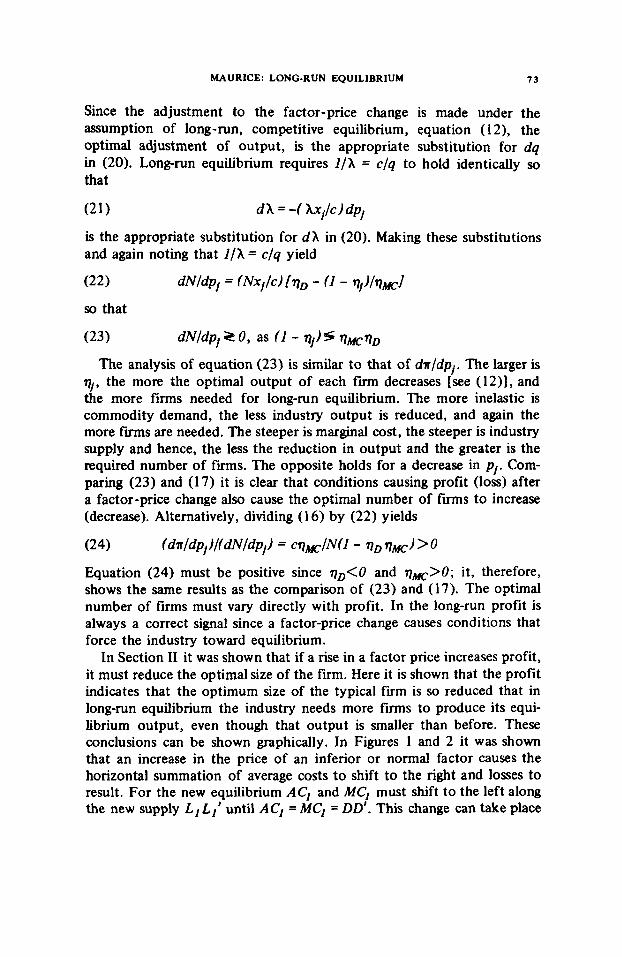
Since the adjustment to the factor-price change is made under the assumption of long-run, competitive equilibrium, equation (1 21, the optimal adjustment of output, is the appropriate substitution for dq in (20). Long-run equilibrium requires I / h = c/q to hold identically so that

(21) dX = 4 x X j / C ) dpj

is the appropriate substitution for d h in (20). Making these substitutions and again noting that I / h = c/q yield

so that

(23) dN/dpi 2 0 , as ( I - qi)S q K q D

The analysis of equation (23) is similar to that of dn/dpi. The larger is qj , the more the optimal output of each fm decreases [see (12)], and the more firms needed for long-run equilibrium. The more inelastic is commodity demand, the less industry output is reduced, and again the more f m s are needed. The steeper is marginal cost, the steeper is industry supply and hence, the less the reduction in output and the greater is the required number of fims. The opposite holds for a decrease in p i . Com- paring (23) and (17) it is clear that conditions causing profit (loss) after a factor-price change also cause the optimal number of f m s to increase (decrease). Alternatively, dividing (1 6) by (22) yields

Equation (24) must be positive since qD<o and q x > O ; it, therefore, shows the same results as the comparison of (23) and (17). The optimal number of firms must vary directly with profit. In the long-run profit is always a correct signal since a factor-price change causes conditions that force the industry toward equilibrium.

In Section I1 it was shown that if a rise in a factor price increases profit, it must reduce the optimal size of the firm. Here it is shown that the profit indicates that the optimum size of the typical firm is so reduced that in long-run equilibrium the industry needs more firms to produce its equilibrium output, even though that output is smaller than before. These conclusions can be shown graphically. In Figures 1 and 2 it was shown that an increase in the price of an inferior or normal factor causes the horizontal summation of average costs to shift to the right and losses to result. For the new equilibrium AC, and MC, must shift to the left along the new supply L, L,' until AC, = MC, = DD'. This change can take place


only through the exit of some firms from the industry. Thus loss signals correctly.

Figure 3 shows that profit can result from a factor-price increase if commodity demand lies between DD' and the vertical line at Qo. Com- petitive equilibrium requires commodity demand to equal AC, = MC1 = L,L, ' . After profit results this can only occur if the entry of new firms causes AC, and MC, to shift to the right along L, L,' . If dd' is commodity demand loss results. In this case, equilibrium requires firms to exit and cause AC, and MC, to shift to the left.

To summarize, for profit to occur after a factor-price increase the optimal output of each fm must diminish so much that the horizontal summation of the average cost curves moves further left than the quantity at which industry supply equals commodity demand. Long-run equilibrium requires a decrease in price and a rightward shift in the horizontal summation of the average cost curves. The only way for these conditions to occur is for new firms to enter the industry. The conditions for loss and exit are similarly explained.

IV. SHORT-RUN EFFECTS AND THE DYNAMIC ADJUSTMENT PATH

There may be dynamic adjustment problems in comparing the speed of entry or exit with the speed of adjustment of existing f m s to their per- ceived long-run target positions. That is, the profit-loss signal after a factor-price change may differ between the short run, in which one or more factors are fixed, and the long run, in which all factors are variable but the number of firms is held constant.

Consider the case in which the first k factors are variable and the remaining (n - k) factors are fixed. If the price of the first factor changes, the profit-loss response in the short run is similar to that set forth in Sec- tion 11, in which all factors were assumed variable. The difference lies in

the different cost function, c = Z p , x , + A , where A is the amount spent

on the fixed factors and in the production function, q = f (XI, x2, . . . , x k ) . The typical firm in short-run equilibrium can be described as follows:

(25) 4 - Alpi = 0

n

i= 1

( i = 1. 2, ..., k<n)

(26) p = I / A '

where I/X' is short-run marginal cost. The expenditure elasticity and the elasticity of marginal cost, derived as above but allowing the usage of only k factors to vary are designated q: and qKk.

Following identically the methods of Section I1 above


Equation (27) does not show the same condition as equation (23) above since qi # qjk and qm f qMk.I2 Therefore, the following condition is conceivable:

Firms, initially in long-run equilibrium, facing a factor-price change and (n - k) fixed factors, given (281, suffer losses. Equations (23) and (28), however, indicate that entry is required for long-run equilibrium. Thus the short-run signal is incorrect. As shown above, if all factors are variable, profit rather than loss results. If short-run (some factors f i e d ) profit occurs when long-run equilibrium requires fewer f m s (or if the opposite situation holds), the short-run profit signal is incorrect, even though the long-run signal indicates correctly.

The situation in which the short- and long-run signals differ is depicted graphically in Figure 4. As above all cost curves are horizontal summations of the cost curves of the firms, the number of f m s held constant. Start- ing from a position of long-run equilibrium at OQo , assume that the price of one of the variable factors increases. Assume also that this factor has

Figure 4

I I 0 00 a

12. Since the slope of ahort-run marginal cost is always steeper than the dope of long-run nur- ginal cost the two elasticities must differ in original long-run equilibrium. If the method# of foot-

note 4 are uwd to coke for it becomes apparent that the two expenditure e b t k i t k d differ because the matrices called /F*/ and /F / in footnote 3 differ between the ahort run and long run. The fint paper IS 1 in this area dealt with increased rent after an increase in the price of a single wiable factor, all other factors fixed. An increase in rent, however, means an i n a e a r in proflt. Roflt is simply rent minus fixed cost; greater rent minus the same fixed cost means greater profit. The condition set forth in IS 1 for an increase in the price of the single variable factor to increase poflt is: Elasticity of Demand < Elasticity of AVC/Elasticity of MC, where elasticity of demand is defined as a positive number. This condition is identical to the condition set forth in equation (27 ) when only one factor is variable. When the ussgea of all but the /-th factor r e fixed 17 = C / p X , where C is total cost, and the elasticity of AVC is (C /p ,x , - I), where the elasticity is evaluated. as above. in long-run equilibrium.

I / I


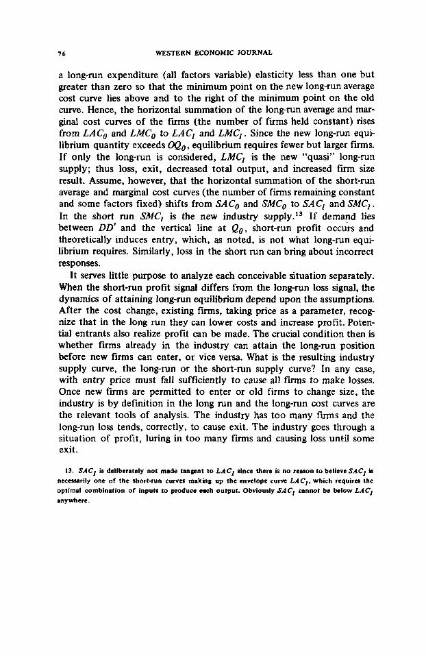
a long-run expenditure (all factors variable) elasticity less than one but greater than zero so that the minimum point on the new long-run average cost curve lies above and to the right of the minimum point on the old curve. Hence, the horizontal summation of the long-run average and marginal cost curves of the f i s (the number of f m s held constant) rises from LACo and LMC, to LACl and LMCI. Since the new long-run equilibrium quantity exceeds oQo , equilibrium requires fewer but larger fms . If only the long-run is considered, LMCl is the new “quasi” long-run supply; thus loss, exit, decreased total output, and increased fm size result. Assume, however, that the horizontal summation of the short-run average and marginal cost curves (the number of firms remaining constant and some factors fixed) shifts from SACo and SMCo to SACl and SMC, . In the short run SMC, is the new industry supply.13 If demand lies between DD’ and the vertical line at Q o , short-run profit occurs and theoretically induces entry, which, as noted, is not what long-run equilibrium requires. Similarly, loss in the short run can bring about incorrect responses.

It serves little purpose to analyze each conceivable situation separately. When the short-run profit signal differs from the long-run loss signal, the dynamics of attaining long-run equilibrium depend upon the assumptions. After the cost change, existing firms, taking price as a parameter, recog- nize that in the long run they can lower costs and increase profit. Poten- tial entrants also realize profit can be made. The crucial condition then is whether firms already in the industry can attain the long-run position before new firms can enter, or vice versa. What is the resulting industry supply curve, the long-run or the short-run supply curve? In any case, with entry price must fall sufficiently to cause all f m s to make losses. Once new firms are permitted to enter or old firms to change size, the industry is by definition in the long run and the long-run cost curves are the relevant tools of analysis. The industry has too many firms and the long-run loss tends, correctly, to cause exit. The industry goes through a situation of profit, luring in too many firms and causing loss unQil some exit.

13. SACl is deliberately not made tangent to LACl since there is no reason to believe SACl ia necessarily one of the short-run curves making up the envelope c u m LACl. which requires the

optimal combination of inputs to produce esch output. Obviously SAC1 cannot be below LAC, anywhere.

MAURICE: LONGRUN EQUILIBRIUM I1

REFERENCES 1. C. E. Ferguson and T. R. Saving, 'Long-Run Adjustment. of a Perfectly Competitive Firm 8nd

Industry," Am. Econ. Rev., Doc. 1969.59, 714-83.

2. P. A. Meyrr, "A Paradox on Profits and Factor Prices," Am. Econ. Rev., June 1967,57,535-41.

3. -, 'A Paradox on Rofitr and Factor Ricer: Reply,' Am. Eoon. Rev., Sopi. 1968, 58, 923-30.

4. J. C. Miller, 111, 'A Paradox on Rofits and Factor Ricer: Comment," Am. Econ. Rev., Wt.

5 . R. R. Nebon, "Inaeawd Kent. from Increased Costs: A Pradox of Value Theory," hour. Pol. Econ.. Oct. 1957, 65, 381-93.

6. P. B. Trescott. 'A Paradox on Rofitr and Factor Rices: Commmt," Am. Econ. Rev., %pi.

1968. 58, 917-19.

1968, 58, 919-23.

FACTOR-PRICE CHANGES, PROFIT, and LONG-RUN EQUILIBRIUM

Documents

Transcript of FACTOR-PRICE CHANGES, PROFIT, and LONG-RUN EQUILIBRIUM