Factor Analysis - Introductionmaitra/stat501/lectures/FactorAnalysis.pdf · Factor Analysis -...
152
Factor Analysis - Introduction • Factor analysis is used to draw inferences on unobservable quantities such as intelligence, musical ability, patriotism, consumer attitudes, that cannot be measured directly. • The goal of factor analysis is to describe correlations between p measured traits in terms of variation in few underlying and unobservable factors. • Changes across subjects in the value of one or more unobserved factors could affect the values of an entire subset of measured traits and cause them to be highly correlated. 654
Transcript of Factor Analysis - Introductionmaitra/stat501/lectures/FactorAnalysis.pdf · Factor Analysis -...

Factor Analysis - Introduction
• Factor analysis is used to draw inferences on unobservable
quantities such as intelligence, musical ability, patriotism,
consumer attitudes, that cannot be measured directly.
• The goal of factor analysis is to describe correlations between
p measured traits in terms of variation in few underlying and
unobservable factors.
• Changes across subjects in the value of one or more
unobserved factors could affect the values of an entire
subset of measured traits and cause them to be highly
correlated.
654
Factor Analysis - Example
• A marketing firm wishes to determine how consumers chooseto patronize certain stores.
• Customers at various stores were asked to complete a surveywith about p = 80 questions.
• Marketing researchers postulate that consumer choices arebased on a few underlying factors such as: friendliness ofpersonnel, level of customer service, store atmosphere,product assortment, product quality and general price level.
• A factor analysis would use correlations among responses tothe 80 questions to determine if they can be grouped into sixsub-groups that reflect variation in the six postulated factors.
655

Orthogonal Factor Model
• X = (X1, X2, . . . , Xp)′ is a p−dimensional vector of
observable traits distributed with mean vector µ andcovariance matrix Σ.
• The factor model postulates that X can be written as a linearcombination of a set of m common factors F1, F2, ..., Fm andp additional unique factors ε1, ε2, ..., εp, so that
X1 − µ1 = `11F1 + `12F2 + · · ·+ `1mFm + ε1X2 − µ2 = `21F1 + `22F2 + · · ·+ `2mFm + ε2
... ...Xp − µp = `p1F1 + `p2F2 + · · ·+ `pmFm + εp
,
where `ij is called a factor loading or the loading of the ithtrait on the jth factor.
656

Orthogonal Factor Model
• In matrix notation: (X−µ)p×1 = Lp×mFm×1 + εp×1, where Lis the matrix of factor loadings and F is the vector of valuesfor the m unobservable common factors.
• Notice that the model looks very much like an ordinary linearmodel. Since we do not observe anything on the right handside, however, we cannot do anything with this model un-less we impose some more structure. The orthogonal factormodel assumes that
E(F) = 0, V ar(F) = E(FF′) = I,
E(ε) = 0, V ar(ε) = E(εε′) = Ψ = diag{ψi}, i = 1, ..., p,
and F, ε are independent, so that Cov(F, ε) = 0.
657

Orthogonal Factor Model• Assuming that the variances of the factors are all one is not
a restriction, as it can be achieved by properly scaling thefactor loadings.
• Assuming that the common factors are uncorrelated and theunique factors are uncorrelated are the defining restrictionsof the orthoginal factor model.
• The assumptions of the orthogonal factor model haveimplications for the structure of Σ. If
(X− µ)p×1 = Lp×mFm×1 + εp×1,
then it follows that
(X− µ)(X− µ)′ = (LF + ε)(LF + ε)′
= (LF + ε)((LF)′+ ε′)= LFF′L′+ εF′L′+ LFε′+ εε′.
658

Orthogonal Factor Model
• Taking expectations of both sides of the equation we find
that:
Σ = E(X− µ)(X− µ)′
= LE(FF′)L′+ E(εF′)L′+ LE(Fε′) + E(εε′)
= LL′+ Ψ,
since E(FF′) = V ar(F) = I and E(εF′) = Cov(ε,F) = 0.
Also,
(X− µ)F′ = LFF′+ εF′,
Cov(X,F) = E[(X− µ)F′] = LE(FF′) + E(εF′) = L.
659

Orthogonal Factor Model
• Under the orthogonal factor model, therefore:
Var(Xi) = σii = `2i1 + `2i2 + · · ·+ `2im + ψi
Cov(Xi, Xk) = σik = `i1`k1 + `i2`k2 + · · ·+ `im`km.
• The portion of the variance σii that is contributed by the m
common factors is the communality and the portion that is
not explained by the common factors is called the uniqueness
(or the specific variance):
σii = `2i1 + `2i2 + · · ·+ `2im + ψi = h2i + ψi.
660

Orthogonal Factor Model
• The model assumes that the p(p+ 1)/2 variances and
covariances of X can be reproduced from the pm + p factor
loadings and the variances of the p unique factors.
• Situations in which m is small relative to p is when factor
analysis works best. If, for example, p = 12 and m = 2, the
78 elements of Σ can be reproduced from 2× 12 + 12 = 36
parameters in the factor model.
• Not all covariance matrices can be factored as LL′+ Ψ.
661

Example: No Proper Solution
• Let p = 3 and m = 1 and suppose that the covariance of
X1, X2, X3 is
Σ =
1 0.9 0.70.9 1 0.40.7 0.4 1
.
• The orthogonal factor model requires that Σ = LL′ + Ψ.
Under the one factor model assumption, we get:
1 = `211 + ψ1 0.90 = `11`21 0.70 = `11`311 = `221 + ψ2 0.40 = `21`31
1 = `231 + ψ3
662

Example: No Proper Solution
• From the equations above, we see that `21 = (0.4/0.7)`11.
• Since 0.90 = `11`21, substituting for `21 implies that `211 =
1.575 or `11 = ±1.255.
• Here is where the problem starts. Since (by assumption)
Var(F1) = 1 and also Var(X1) = 1, and since therefore
Cov(X1, F1) = Corr(X1, F1) = `11, we notice that we have a
solution inconsistent with the assumptions of the model be-
cause a correlation cannot be larger than 1 or smaller than
-1.
663

Example: No Proper Solution
• Further,
1 = `211 + ψ1 −→ ψ1 = 1− `211 = −0.575,
which cannot be true because ψ = Var(ε1). Thus, for m = 1
we get a numerical solution that is not consistent with the
model or with the interpretation of its parameters.
664
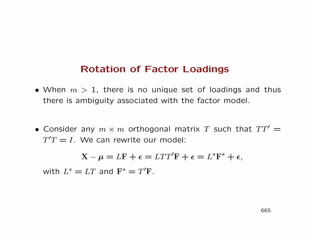
Rotation of Factor Loadings
• When m > 1, there is no unique set of loadings and thus
there is ambiguity associated with the factor model.
• Consider any m × m orthogonal matrix T such that TT ′ =
T ′T = I. We can rewrite our model:
X− µ = LF + ε = LTT ′F + ε = L∗F∗+ ε,
with L∗ = LT and F∗ = T ′F.
665

Rotation of Factor Loadings
• Since
E(F∗) = T ′E(F) = 0, and Var(F∗) = T′Var(F)T = T′T = I,
it is impossible to distinguish between loadings L and L∗
from just a set of data even though in general they will be
different.
• Notice that the two sets of loadings generate the same co-
variance matrix Σ:
Σ = LL′+ Ψ = LTT ′L′+ Ψ = L∗L∗′+ Ψ.
666
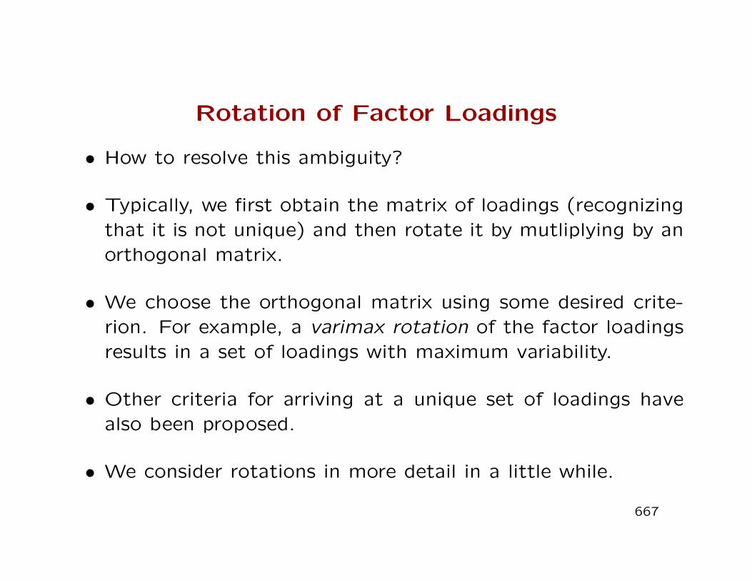
Rotation of Factor Loadings
• How to resolve this ambiguity?
• Typically, we first obtain the matrix of loadings (recognizingthat it is not unique) and then rotate it by mutliplying by anorthogonal matrix.
• We choose the orthogonal matrix using some desired crite-rion. For example, a varimax rotation of the factor loadingsresults in a set of loadings with maximum variability.
• Other criteria for arriving at a unique set of loadings havealso been proposed.
• We consider rotations in more detail in a little while.
667

Estimation in Orthogonal Factor Models
• We begin with a sample of size n of p−dimensional vectorsx1, x2, ..., xn and (based on our knowledge of the problem)choose a small number m of factors.
• For the chosen m, we want to estimate the factor loadingmatrix L and the specific variances in the model
Σ = LL′+ Ψ
• We use S as an estimator of Σ and first investigate whetherthe correlations among the p variables are large enough tojustify the analysis. If rij ≈ 0 for all i, j, the unique factorsψi will dominate and we will not be able to identify commonunderlying factors.
668

Estimation in Orthogonal Factor Models
• Common estimation methods are:
– The principal component method
– The iterative principal factor method
– Maximum likelihood estimation (assumes normaility)
• The last two methods focus on using variation in common
factors to describe correlations among measured traits. Prin-
cipal component analysis gives more attention to variances.
• Estimated factor loadings from any of those methods can
be rotated, as explained later, to facilitate interpretation of
results.
669

The Principal Component Method
• Let (λi, ei) denote the eigenvalues and eigenvectors of Σ andrecall the spectral decomposition which establishes that
Σ = λ1e1e′1 + λ2e2e
′2 + · · ·+ λpepe
′p.
• Use L to denote the p×p matrix with columns equal to√λiei,
i = 1, ..., p. Then the spectral decomposition of Σ is givenby
Σ = LL′+ 0 = LL′,
and corresponds to a factor model in which there are as manyfactors as variables m = p and where the specific variancesψi = 0. The loadings on the jth factor are just the coeffi-cients of the jth principal component multiplied by
√λj.
670

The Principal Component Method
• The principal component solution just described is not
interesting because we have as many factors as we have
variables.
• We really want m < p so that we can explain the covariance
structure in the measurements using just a small number of
underlying factors.
• If the last p−m eigenvalues are small, we can ignore the last
p−m terms in the spectral decomposition and write
Σ ≈ Lp×mL′m×p.
671

The Principal Component Method
• The communality for the i-th observed variable is the amountof its variance that can be atttributed to the variation in them factors
hi =m∑j=1
`2ij for i = 1,2, ..., p
• The variances ψi of the specific factors can then be taken tobe the diagonal elements of the difference matrix Σ − LL′,where L is p×m. That is,
ψi = σii −m∑j=1
`2ij for i = 1, ..., p
or Ψ = diag(Σ− Lp×mL′m×p)
672

The Principal Component Method
• Note that using m < p factors will produce an approximation
Lp×mL′m×p + Ψ
for Σ that exactly reproduces the variances of the p measured
traits but only approximates the correlations.
• If variables are measured in very different scales, we work
with the standardized variables as we did when extracting
PCs. This is equivalent to modeling the correlation matrix
P rather than the covariance matrix Σ.
673

Principal Component Estimation
• To implement the PC method, we must use S to estimate
Σ (or use R if the observations are standardized) and use X
to estimate µ.
• The principal component estimate of the loading matrix for
the m factor model is
L = [√λ1e1
√λ2e2 ...
√λmem],
where (λi, ei) are the eigenvalues and eigenvectors of S (or
of R if the observations are standardized).
674

Principal Component Estimation
• The estimated specific variances are given by the diagonalelements of S − LL′, so
Ψ =
ψ1 0 · · · 00 ψ2 · · · 0... ... ... ...0 0 · · · ψp
, ψi = sii −m∑j=1
˜2ij.
• Communalities are estimated as
h2i = ˜2
i1 + ˜2i2 + · · ·+ ˜2
im.
• If variables are standardized, then we substitute R for S andsubstitute 1 for each sii.
675

Principal Component Estimation
• In many applications of factor analysis, m, the number offactors, is decided prior to the analysis.
• If we do not know m, we can try to determine the ’best’ mby looking at the results from fitting the model with differentvalues for m.
• Examine how well the off-diagonal elements of S (or R) arereproduced by the fitted model LL′+Ψ because by definitionof ψi, diagonal elements of S are reproduced exactly but theoff-diagonal elements are not. The chosen m is appropriateif the residual matrix
S − (LL′+ Ψ)
has small off-diagonal elements.
676

Principal Component Estimation
• Another approach to deciding on m is to examine the
contribution of each potential factor to the total variance.
• The contribution of the k-th factor to the sample variance
for the i-th trait, sii, is estimated as ˜2ik.
• The contribution of the k-th factor to the total sample
variance s11 + s22 + ...+ spp is estimated as
˜21k + ˜2
2k + ...+ ˜2pk = (
√λkek)′(
√λkek) = λk.
677

Principal Component Estimation
• As in the case of PCs, in general(Proportion of total samplevariance due to jth factor
)=
λj
s11 + s22 + · · ·+ spp,
or equals λj/p if factors are extracted from R.
• Thus, a ’reasonable’ number of factors is indicated by
the minimum number of PCs that explain a suitably large
proportion of the total variance.
678

Strategy for PC Factor Analysis
• First, center observations (and perhaps standardize)
• If m is determined by subject matter knowledge, fit the mfactor model by:
– Extracting the p PCs from S or from R.
– Constructing the p × m matrix of loadings L by keepingthe PCs associated to the largest m eigenvalues of S (orR).
• If m is not known a priori, examine the estimatedeignevalues to determine the number of factors thataccount for a suitably large proportion of the totalvariance and examine the off-diagonal elements of theresidual matrix.
679

Example: Stock Price Data
• Data are weekly gains in stock prices for 100 consecutive
weeks for five companies: Allied Chemical, Du Pont, Union
Carbide, Exxon and Texaco.
• Note that the first three are chemical companies and the last
two are oil companies.
• The data are first standardized and the sample correlation
matrix R is computed.
• Fit an m = 2 orthogonal factor model
680

Example: Stock Price Data
• The sample correlation matrix R is
R =
1 0.58 0.51 0.39 0.46
1 0.60 0.39 0.321 0.44 0.42
1 0.521
.
• Eigenvalues and eigenvectors of R are
λ =
2.860.810.540.450.34
, e1 =
0.4640.4570.4700.4160.421
, e2 =
−0.241−0.509−0.261
0.5250.582
.
681

Example: Stock Price Data
• Recall that the method of principal components results infactor loadings equal to
√λej, so in this case
Loadings Loadings Specificon factor 1 on factor 2 variances
Variable ˜i1 ˜i2 ψi = 1− h2i
Allied Chem 0.784 -0.217 0.34Du Pont 0.773 -0.458 0.19
Union Carb 0.794 -0.234 0.31Exxon 0.713 0.472 0.27Texaco 0.712 0.524 0.22
• The proportions of total variance accounted by the first andsecond factors are λ1/p = 0.571 and λ2/p = 0.162.
682

Example: Stock Price Data
• The first factor appears to be a market-wide effect on weekly
stock price gains whereas the second factor reflects industry
specific effects on chemical and oil stock price returns.
• The residual matrix is given by
R− (LL′+ Ψ) =
0 −0.13 −0.16 −0.07 0.02
0 −0.12 0.06 0.010 −0.02 −0.02
0 −0.230
.
• By construction, the diagonal elements of the residual matrix
are zero. Are the off-diagonal elements small enough?
683

Example: Stock Price Data
• In this example, most of the residuals appear to be small,with the exception of the {4,5} element and perhaps alsothe {1,2}, {1,3}, {2,3} elements.
• Since the {4,5} element of the residual matrix is negative,we know that LL′ is producing a correlation value betweenExxon and Texaco that is larger than the observed value.
• When the off-diagonals in the residual matrix are not small,we might consider changing the number m of factors to seewhether we can reproduce the correlations between the vari-ables better.
• In this example, we would probably not change the model.
684

SAS code: Stock Price Data
/* This program is posted as stocks.sas. It performs
factor analyses for the weekly stock return data from
Johnson & Wichern. The data are posted as stocks.dat */
data set1;
infile "c:\stat501\data\stocks.dat";
input x1-x5;
label x1 = ALLIED CHEM
x2 = DUPONT
x3 = UNION CARBIDE
x4 = EXXON
x5 = TEXACO;
run;
685

/* Compute principal components */
proc factor data=set1 method=prin scree nfactors=2
simple corr ev res msa nplot=2
out=scorepc outstat=facpc;
var x1-x5;
run;
Factor Pattern
Factor1 Factor2
x1 ALLIED CHEM 0.78344 -0.21665
x2 DUPONT 0.77251 -0.45794
x3 UNION CARBIDE 0.79432 -0.23439
x4 EXXON 0.71268 0.47248
x5 TEXACO 0.71209 0.52373
686

R code: Stock Price Data
# This code creates scatter plot matrices and does
# factor analysis for 100 consecutive weeks of gains
# in prices for five stocks. This code is posted as
#
# stocks.R
#
# The data are posted as stocks.dat
#
# There is one line of data for each week and the
# weekly gains are represented as
# x1 = ALLIED CHEMICAL
# x2 = DUPONT
# x3 = UNION CARBIDE
# x4 = EXXON
# x5 = TEXACO
687

stocks <- read.table("c:/stat501/data/stocks.dat", header=F,
col.names=c("x1", "x2", "x3", "x4", "x5"))
# Print the first six rows of the data file
stocks[1:6, ]
x1 x2 x3 x4 x5
1 0.000000 0.000000 0.000000 0.039473 0.000000
2 0.027027 -0.044855 -0.003030 -0.014466 0.043478
3 0.122807 0.060773 0.088146 0.086238 0.078124
4 0.057031 0.029948 0.066808 0.013513 0.019512
5 0.063670 -0.003793 -0.039788 -0.018644 -0.024154
6 0.003521 0.050761 0.082873 0.074265 0.049504
688

# Create a scatter plot matrix of the standardized data
stockss <- scale(stocks, center=T, scale=T)
pairs(stockss,labels=c("Allied","Dupont","Carbide", "Exxon",
"Texaco"), panel=function(x,y){panel.smooth(x,y)
abline(lsfit(x,y),lty=2) })
689

Allied
−2 0 1 2 3
●
●
●
●●
●
●
●
●● ●
●
●
●
●
●●
●
●
●●●
●●
●
●
●●
●
●
●
●●●●
●
●
●
●
●
●●
●
●●
●
●●
●
●
●
●
●
●
●
●
●
● ●
●
●●
●
●
●
●●
●
●
●
●●
●
●
●
●
●
●
●
●
●
●
●●
●
●●
●
●
●
●
●
●
●
●
●
●
●●
●●
●
●
●●
●
●
●
●●●
●
●
●
●
●●
●
●
●● ●
●●
●
●
●●
●
●
●
●●●●
●
●
●
●
●
●●
●
●●
●
●●
●
●
●
●
●
●
●
●
●
●●
●
●●
●
●
●
●●
●
●
●
●●
●
●
●
●
●
●
●
●
●
●
●●
●
●●
●
●
●
●
●
●
●
●
●
●
●●
●
−2 0 1 2 3
●
●
●
●●
●
●
●
●● ●
●
●
●
●
●●
●
●
●● ●
● ●
●
●
●●
●
●
●
●●●●
●
●
●
●
●
●●
●
●●
●
●●
●
●
●
●
●
●
●
●
●
●●
●
●●
●
●
●
●●
●
●
●
●●
●
●
●
●
●
●
●
●
●
●
●●
●
●●
●
●
●
●
●
●
●
●
●
●
●●
●
−2
01
23
●
●
●
●●
●
●
●
●●●
●
●
●
●
● ●
●
●
●● ●
●●
●
●
●●
●
●
●
●●●●
●
●
●
●
●
●●
●
●●
●
●●
●
●
●
●
●
●
●
●
●
● ●
●
●●
●
●
●
●●
●
●
●
●●
●
●
●
●
●
●
●
●
●
●
●●
●
●●
●
●
●
●
●
●
●
●
●
●
●●
●
−2
01
23
●
●
●
●
●
●
●
●
●●
●●
●
●
●
●
●
●
●
●●●
●
●
●
●
● ●●
●
●
●
●
●●●
●
●●
●●
●
●
●
●● ●
●● ●
●
●
●
●●
●
●
●●
●
●
●
●
●
●
●●
●
● ●●●
●
●
●
●●
●
●●
●
●
●
●
● ●
●
●
●
●●
●
●
●
●●
● ●●
●
Dupont●
●
●
●
●
●
●
●
●●
●●
●
●
●
●
●
●
●
●● ●
●
●
●
●
● ●●
●
●
●
●
●● ●
●
●●
●●
●
●
●
●● ●
●●●
●
●
●
●●
●
●
●●
●
●
●
●
●
●
●●
●
●●●●
●
●
●
●●
●
●●
●
●
●
●
●●
●
●
●
●●
●
●
●
●●
● ●●
●
●
●
●
●
●
●
●
●
●●
●●
●
●
●
●
●
●
●
●● ●
●
●
●
●
● ●●
●
●
●
●
●● ●
●
●●
●●
●
●
●
●● ●
●● ●
●
●
●
●●
●
●
●●
●
●
●
●
●
●
● ●
●
●●●●
●
●
●
●●
●
●●
●
●
●
●
● ●
●
●
●
●●
●
●
●
●●
● ●●
●
●
●
●
●
●
●
●
●
●●
●●
●
●
●
●
●
●
●
●● ●
●
●
●
●
● ●●
●
●
●
●
●● ●
●
●●
●●
●
●
●
●●●
●● ●
●
●
●
●●
●
●
●●
●
●
●
●
●
●
●●
●
● ●●●
●
●
●
●●
●
●●
●
●
●
●
● ●
●
●
●
●●
●
●
●
●●
●●●
●
● ●
●
●
●
●
●
●
●●
●
●
●
●●●
●
●
●●
●
●
●
●
●
●
●
●
●
●
●
●
●
●
●
●
●
● ●
●
●
●
●●
●
●
●
●
● ●
●
●●
●
●
●
●
●●●
●●●
●
●
●●
●
●●
●●
●
●
●
●
●
●●●
●
●
●
●
● ●
●
● ●
●
●
●
●
●●
●●
●
●●●●
●
●
●
●
●
●
●●
●
●
●
●●●
●
●
●●
●
●
●
●
●
●
●
●
●
●
●
●
●
●
●
●
●
●●
●
●
●
●●
●
●
●
●
●●
●
●●
●
●
●
●
● ●●
●●●
●
●
●●
●
●●
●●
●
●
●
●
●
●●●
●
●
●
●
●●
●
●●
●
●
●
●
●●
●●
●
●● Carbide ●●
●
●
●
●
●
●
●●
●
●
●
●●●
●
●
●●
●
●
●
●
●
●
●
●
●
●
●
●
●
●
●
●
●
●●
●
●
●
●●
●
●
●
●
● ●
●
●●
●
●
●
●
●● ●
●●●
●
●
●●
●
●●
●●
●
●
●
●
●
●●●
●
●
●
●
● ●
●
● ●
●
●
●
●
●●
●●
●
● ●
−2
01
2
● ●
●
●
●
●
●
●
●●
●
●
●
●●●
●
●
●●
●
●
●
●
●
●
●
●
●
●
●
●
●
●
●
●
●
●●
●
●
●
●●
●
●
●
●
● ●
●
●●
●
●
●
●
● ●●
● ●●
●
●
●●
●
●●
●●
●
●
●
●
●
●●●
●
●
●
●
● ●
●
●●
●
●
●
●
●●
●●
●
●●
−2
01
23
●
●
●
●
●
●
● ●
●
●
●
●
●
●●
●
●
●●
●
●
●
●
●
●
●
●
●●
●
●●
●●●
●
●
●
●●
●●
●
●●●
● ●
●
●
●●
●●●
●
●
●●
●
●
●
●
●
●
●
●
●
● ●
●
●
●
●
●●
●
●
●
●
●●
●
●
●
●
●
●
● ●●●
●
●
●
●
●
●
●
●●
●
●
●
●
●
● ●
●
●
●
●
●
●●
●
●
●●
●
●
●
●
●
●
●
●
●●
●
●●
●●●
●
●
●
●●
●●
●
●●●
● ●
●
●
●●
●●●
●
●
●●
●
●
●
●
●
●
●
●
●
●●
●
●
●
●
●●
●
●
●
●
●●
●
●
●
●
●
●
● ●●●
●
●
●
●
●
●
●
●●
●
●
●
●
●
● ●
●
●
●
●
●
●●
●
●
●●
●
●
●
●
●
●
●
●
●●
●
●●
●●
●
●
●
●
●●
●●
●
● ●●
● ●
●
●
●●
●●●
●
●
●●
●
●
●
●
●
●
●
●
●
●●
●
●
●
●
●●
●
●
●
●
●●
●
●
●
●
●
●
● ●●●
●
●
●
●
●
●
●
●
Exxon●
●
●
●
●
●
● ●
●
●
●
●
●
●●
●
●
●●
●
●
●
●
●
●
●
●
●●
●
●●
●●
●
●
●
●
●●
●●
●
● ●●
● ●
●
●
●●
●●●
●
●
●●
●
●
●
●
●
●
●
●
●
● ●
●
●
●
●
●●
●
●
●
●
●●
●
●
●
●
●
●
● ●●●
●
●
●
●
●
●
●
●
−2 0 1 2 3
●
●
●
●
●
●
●
●
●●
●
●
● ●
●●
●
●●
●
●
● ●
●
●
●
●
●● ●●
●
●●●
●
●
●
●
●
●
●
●
●
●
●
●
●●
●
●
●
●
●
●
●
●
●
●●●
●
●
●
●●
●●
●
●
●●
●●● ●
●
●●
●
●●
●
●●
●●
●
●
●●
●
●
●
●
●
●●●● ●
●
●
●
●
●
●
●
●●
●
●
●●
●●
●
●●
●
●
● ●
●
●
●
●
●● ●●
●
●●●
●
●
●
●
●
●
●
●
●
●
●
●
●●
●
●
●
●
●
●
●
●
●
●●●
●
●
●
●●
●●
●
●
●●
●●● ●
●
●●
●
●●
●
●●
●●
●
●
●●
●
●
●
●
●
●●
●●
−2 0 1 2
●
●
●
●
●
●
●
●
●●
●
●
●●
●●
●
●●
●
●
● ●
●
●
●
●
●● ●●
●
●●
●
●
●
●
●
●
●
●
●
●
●
●
●
●●
●
●
●
●
●
●
●
●
●
●●●
●
●
●
●●
●●
●
●
●●
●●● ●
●
●●
●
●●
●
●●
●●
●
●
●●
●
●
●
●
●
●●
●● ●
●
●
●
●
●
●
●
●●
●
●
●●
●●
●
●●
●
●
●●
●
●
●
●
●● ●●
●
●●
●
●
●
●
●
●
●
●
●
●
●
●
●
●●
●
●
●
●
●
●
●
●
●
● ●●
●
●
●
●●
●●
●
●
●●
●● ●●
●
●●
●
●●
●
●●
●●
●
●
●●
●
●
●
●
●
●●
● ●
−2 0 1 2 3
−2
01
23
Texaco
690

# Compute principal components from the correlation matrix
s.cor <- var(stockss)
s.cor
x1 x2 x3 x4 x5
x1 1.0000000 0.5769308 0.5086555 0.3867206 0.4621781
x2 0.5769308 1.0000000 0.5983817 0.3895188 0.3219545
x3 0.5086555 0.5983817 1.0000000 0.4361014 0.4256266
x4 0.3867206 0.3895188 0.4361014 1.0000000 0.5235293
x5 0.4621781 0.3219545 0.4256266 0.5235293 1.0000000
s.pc <- prcomp(stocks, scale=T, center=T)
# List component coefficients
691

s.pc$rotation
PC1 PC2 PC3 PC4 PC5
x1 0.4635414 -0.2408580 0.6133475 -0.3813591 0.4533066
x2 0.4570769 -0.5090981 -0.1778906 -0.2113173 -0.6749813
x3 0.4699796 -0.2605708 -0.3370501 0.6641056 0.3957057
x4 0.4216766 0.5252677 -0.5390141 -0.4728058 0.1794471
x5 0.4213290 0.5822399 0.4336136 0.3812200 -0.3874650

# Estimate proportion of variation explained by each
# principal component,and cummulative proportions
s <- var(s.pc$x)
pvar<-round(diag(s)/sum(diag(s)), digits=6)
pvar
PC1 PC2 PC3 PC4 PC5
0.571298 0.161824 0.108008 0.090270 0.068600
cpvar <- round(cumsum(diag(s))/sum(diag(s)), digits=6)
cpvar
PC1 PC2 PC3 PC4 PC5
0.571298 0.733122 0.841130 0.931400 1.000000
692

# Plot component scores
par(fin=c(5,5))
plot(s.pc$x[,1],s.pc$x[,2],
xlab="PC1: Overall Market",
ylab="PC2: Oil vs. Chemical",type="p")
693

●
●●
●
●
●
●
●
●
●
●
●
●
●
●
●
●
●
●
●
●
●
●●
●
●
●
●
●
●
●
●
●
●●
●
●●
●
●
●
●
●●
●
●●
●
●
●
●
●
●
●●
●
●● ●
●●
●
●
●
●
●●
●
●●
●●
●
●
●
●
●●●
●
●
●
●
●
●
●
●
●
●
●
●
●
● ●
●●
●
●●
●
−4 −2 0 2 4
−2
−1
01
23
PC1: Overall Market
PC
2: O
il vs
. Che
mic
al

Principal Factor Method
• The principal factor method for estimating factor loadingscan be viewed as an iterative modification of the principalcomponents methods that allows for greater focus onexplaining correlations among observed traits .
• The principal factor approach begins with a guess about thecommunalities and then iteratively updates those estimatesuntil some convergence criterion is satisfied. (Try severaldifferent sets of starting values.)
• The principal factor method chooses factor loadings thatmore closely reproduce correlations. Principal componentsare more heavily influenced by accounting for variances andwill explain a higher proportion of the total variance.
694
Principal Factor Method
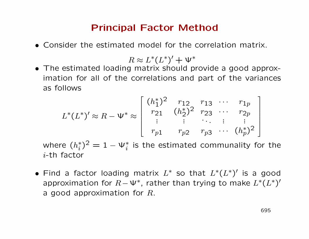
• Consider the estimated model for the correlation matrix.
R ≈ L∗(L∗)′+ Ψ∗
• The estimated loading matrix should provide a good approx-imation for all of the correlations and part of the variancesas follows
L∗(L∗)′ ≈ R−Ψ∗ ≈
(h∗1)2 r12 r13 · · · r1pr21 (h∗2)2 r23 · · · r2p
... ... . . . ... ...rp1 rp2 rp3 · · · (h∗p)
2
where (h∗i )
2 = 1 −Ψ∗i is the estimated communality for thei-th factor
• Find a factor loading matrix L∗ so that L∗(L∗)′ is a goodapproximation for R−Ψ∗, rather than trying to make L∗(L∗)′
a good approximation for R.
695

Principal Factor Method
• Start by obtaining initial estimates of the communalities,(h∗1)2, (h∗2)2, ..., (h∗p)
2.
• Then the estimated loading matrix should provide a goodapproximation to
R−Ψ∗ ≈
(h∗1)2 r12 r13 · · · r1pr21 (h∗2)2 r23 · · · r2p
... ... . . . ... ...rp1 rp2 rp3 · · · (h∗p)
2
where (h∗i )
2 = 1 −Ψ∗i is the estimated communality for thei-th factor
• Use the spectral decomposition of R − Ψ∗ to find a goodapproximation to R−Ψ∗.
696

Principal Factor Method
• Use the initial estimates to compute
R−Ψ∗ ≈
(h∗1)2 r12 r13 · · · r1pr21 (h∗2)2 r23 · · · r2p
... ... . . . ... ...rp1 rp2 rp3 · · · (h∗p)
2
The estimated loading matrix is obtained from the eigneval-ues and eigenvectors of this matrix as
L∗ =[√λ∗1e∗1 · · · ·
√λ∗me∗m
]
• Update the specific variances
Ψ∗i = 1−m∑j=1
λ∗j [e∗ij]
2
697

Principal Factor Method
• Use the updated communalities to re-evaluate
R−Ψ∗ ≈
(h∗1)2 r12 r13 · · · r1pr21 (h∗2)2 r23 · · · r2p
... ... . . . ... ...rp1 rp2 rp3 · · · (h∗p)
2
and compute a new estimate of the loading matirx,
L∗ =[√λ∗1e∗1 · · · ·
√λ∗me∗m
]
• Repeat this process until it converges.
698
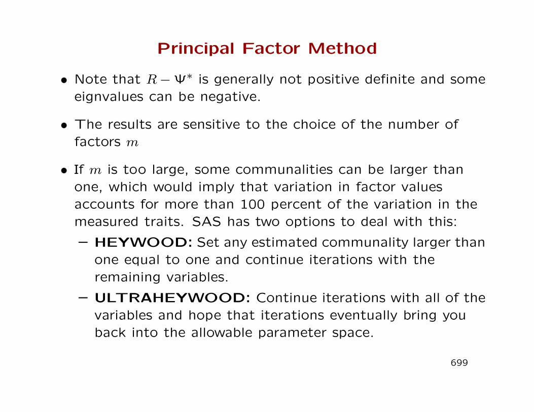
Principal Factor Method
• Note that R−Ψ∗ is generally not positive definite and someeignvalues can be negative.
• The results are sensitive to the choice of the number offactors m
• If m is too large, some communalities can be larger thanone, which would imply that variation in factor valuesaccounts for more than 100 percent of the variation in themeasured traits. SAS has two options to deal with this:
– HEYWOOD: Set any estimated communality larger thanone equal to one and continue iterations with theremaining variables.
– ULTRAHEYWOOD: Continue iterations with all of thevariables and hope that iterations eventually bring youback into the allowable parameter space.
699

Stock Price Example
• The estimated loadings from the principal factor method aredisplayed below.
Loadings Loadings Specific Commu-on factor 1 on factor 2 variances nalities
Variable `∗i1 `∗i2 ψ∗i = 1− (h∗i )2 (h∗i )
2
Allied Chem 0.70 -0.09 0.50 0.50Du Pont 0.71 -0.25 0.44 0.56
Union Carb 0.72 -0.11 0.47 0.53Exxon 0.62 0.23 0.57 0.43Texaco 0.62 0.28 0.54 0.46
• The proportions of total variance accounted by the first andsecond factors are λ∗1/p = 0.45 and λ∗2/p = 0.04.
700

Stock Price Example
• Interpretations are similar. The first factor appears to be a
market-wide effect on weekly stock price gains whereas the
second factor reflects industry specific effects on chemical
and oil stock price returns.
• The loadings tend to be smaller than those obtained from
principal component analysis. Why?
701

Stock Price Example
• The residual matrix is
R−[(L∗)(L∗)′+Ψ∗] =
0 0.057 −0.005 −0.029 0.053
0 0.060 0.007 −0.0490 0.015 0.010
0 0.0730
.
• Since the principal factor methods give greater emphasis
to describing correlations, the off-diagonal elements of
the residual matrix tend to be smaller than corresponding
elements for principal component estimation.
702

/* SAS code for the principal factor method */
proc factor data=set1 method=prinit scree nfactors=2
simple corr ev res msa nplot=2
out=scorepf outstat=facpf;
var x1-x5;
priors smc;
run;
To obtain the initial communaliy for the i-th variable, ”smc” in
the priors statement uses the R2 value for the regression of the
i-th variable on the other p− 1 variables in the analysis.
703

Maximum Likelihood Estimation
• To implement the ML method, we need to include someassumptions about the distribution of the p-dimensionalvector Xj and the m-dimensional vector Fj:
Xj ∼ Np(µ,Σ), Fj ∼ Nm(0, Im), εj ∼ Np(0,Ψp×p),
where Xj = LFj + εj, Σ = LL′+ Ψ, and Fj is independent ofεj . Also, Ψ is a diagonal matrix.
• Because the L that maximizes the likelihood for this modelis not unique, we need another set of restrictions that leadto a unique maximum of the likelihood function:
L′Ψ−1L = ∆,
where ∆ is a diagonal matrix.
704

Maximum Likelihood Estimation
• Maximizing the likelihood function with respect to (µ,L,Ψ) is
not easy because the likelihood depends in a very non-linear
fashion on the parameters.
• Recall that (L,Ψ) enter the likelihood through Σ which in
turn enters the likelihood as an inverse matrix in a quadratic
form and also as a determinant.
• Efficient numerical algorithms exist to maximize the
likelihood iteratively and obtain ML estimates
Lm×m = {ˆij}, Ψ = diag{ψi}, µ = x.
705

Maximum Likelihood Estimation
• The MLEs of the communalities for the p variables (with m
factors)are
h2i =
m∑j=1
ˆ2ij, i = 1, ..., p,
and the proportion of the total variance accounted for by the
jth factor is given by∑pi=1
ˆ2ij
trace(S)if using S
or dividing by p if using R.
706

Maximum Likelihood Estimation: Stock Prices
• Results;
Loadings Loadings SpecificVariable for factor 1 for factor 2 variances
Allied Chem 0.684 0.189 0.50Du Pont 0.694 0.517 0.25
Union Carb. 0.681 0.248 0.47Exxon 0.621 -0.073 0.61Texaco 0.792 -0.442 0.18
Prop. of variance 0.485 0.113
707

Maximum Likelihood Estimation: Stock Prices
• The interpretation of the two factors remains more or less
the same (although Exxon is hardly loading on the second
factor now).
• What has improved considerably is the residual matrix, since
most of the entries are essentially zero now:
R− (LL′+ Ψ) =
0 0.005 −0.004 −0.024 −0.004
0 −0.003 −0.004 0.0000 0.031 −0.004
0 −0.0000
.
708

Likelihood Ratio test for Number of Factors
• We wish to test whether the m factor model appropriatelydescribes the covariances among the p variables.
• We test
H0 : Σp×p = Lp×mL′m×p + Ψp×p
versus
Ha : Σ is a positive definite matrix
• A likelihood ratio test for H0 can be constructed as the ratioof the maximum of likelihood function under H0 and themaximum of the likelihood function under no restrictions(i.e., under Ha).
709

Likelihood Ratio test for Number of Factors
• Under Ha the multivariate normal likelihood is maximized at
µ = x, and Σ = 1n
∑ni=1(xi − x)(xi − x)′.
• Under H0, the multivariate normal likelihood is maximized at
µ = x and LL′+ Ψ, the mle for Σ for the orthogonal factor
model with m factors.
710

Likelihood Ratio test for Number of Factors
• It is easy to show that the result is proportional to
|LL′+ Ψ|−n/2 exp(−
1
2ntr[(LL′+ Ψ)−1Σ]
),
Then, the log-likelihood ratio statistic for testing H0 is
−2 ln Λ = −2 ln
(|LL′+ Ψ||Σ|
)−n/2
+ n[tr((LL′+ Ψ)−1Σ)− p].
• Since the second term in the expression above can be shown
to be zero, the test statistic simplifies to
−2 ln Λ = n ln
(|LL′+ Ψ||Σ|
).
711

Likelihood Ratio test for Number of Factors
• The degrees of freedom for the large sample chi-square
approximation to this test statistic are
(1/2)[(p−m)2 − p−m]
Where does this come from?
• Under Ha we estimate p means and p(p+1)/2 elements of Σ.
• Under H0, we estimate p means p diagonal elements of Ψ
and mp elements of L.
• An additional set of m(m − 1)/2 restrictions are imposed
on the mp elements of L by the identifiability restriction
L′Ψ−1L = ∆712

Likelihood Ratio test for Number of Factors
• Putting it all together, we have
df = [p+p(p+ 1)
2]−[p+pm+p−
m(m− 1)
2] =
1
2[(p−m)2−p−m]
degrees of freedom.
• Bartlett showed that the χ2 approximation to the sampling
distribution of −2 ln Λ can be improved if the test statistic is
computed as
−2 ln Λ = (n− 1− (2p+ 4m+ 5)/6) ln|LL′+ Ψ||Σ|
.
713

Likelihood Ratio test for Number of Factors
• We reject H0 at level α if
−2 ln Λ = (n− 1− (2p+ 4m+ 5)/6) ln|LL′+ Ψ||Σ|
> χ2df ,
with df = 12[(p−m)2 − p−m] for large n and large n− p.
• To have df > 0, we must have m < 12(2p+ 1−
√8p+ 1).
• If the data are not a random sample from a multivariate
normal distribution, this test tends to indicate the need for
too many factors.
714

Stock Price Data
• We carry out the log-likelihood ratio test at level α = 0.05
to see whether the two-factor model is appropriate for these
data.
• We have estimated the factor loadings and the unique factors
using R rather than S, but the exact same test statistic (with
R in place of Σ) can be used for the test.
• Since we evaluated L, Ψ and R, we can easily compute
|LL′+ Ψ||R|
=0.194414
0.193163= 1.0065.
715

Stock Price Data
• Then, the test statistic is
[100− 1−(10 + 8 + 5)
6] ln(1.0065) = 0.58.
• Since 0.58 < χ21 = 3.84, we fail to reject H0 and conclude
that the two-factor model adequately describes the
correlations among the five stock prices (p-value=0.4482).
• Another way to say it is that the data do not contradict the
two-factor model.
716

Stock Price Data
• Test the null hypothesis that one factor is sufficient
[100− 1−(10 + 4 + 5)
6] ln|LL′+ Ψ||Σ|
= 15.49
with 5 degrees of freedom.
• Since p − value = 0.0085, we reject the null hypothesis and
conclude that a one factor model is not sufficient to describe
the correlations among the weekly returns for the five stocks.
717

Maximum Likelihood Estimation: Stock Prices
• We implemented the ML method for the stock price example.
• The same SAS program can be used, but now use ’method
= ml’ instead of ’prinit’ in the proc factor statement.
proc factor data=set1 method=ml scree nfactors=2
simple corr ev res msa nplot=2
out=scorepf outstat=facpf;
var x1-x5; priors smc;
run;
718

Initial Factor Method: Maximum Likelihood
Prior Communality Estimates: SMC
x1 x2 x3 x4 x5
0.43337337 0.46787840 0.44606336 0.34657438 0.37065882
Preliminary Eigenvalues: Total = 3.56872 Average = 0.713744
Eigenvalue Difference Proportion Cumulative
1 3.93731304 3.59128674 1.1033 1.1033
2 0.34602630 0.42853688 0.0970 1.2002
3 -.08251059 0.15370829 -0.0231 1.1771
4 -.23621888 0.15967076 -0.0662 1.1109
5 -.39588964 -0.1109 1.0000
2 factors will be retained by the NFACTOR criterion.
719

Iteration Criterion Ridge Change Communalities
1 0.0160066 0.0000 0.4484 0.49395 0.74910 0.52487
0.28915 0.81911
2 0.0060474 0.0000 0.1016 0.50409 0.74984 0.52414
0.39074 0.82178
3 0.0060444 0.0000 0.0014 0.50348 0.74870 0.52547
0.39046 0.82316
4 0.0060444 0.0000 0.0004 0.50349 0.74845 0.52555
0.39041 0.82357
5 0.0060444 0.0000 0.0001 0.50349 0.74840 0.52557
0.39038 0.82371
6 0.0060444 0.0000 0.0000 0.50349 0.74839 0.52557
0.39037 0.82375
Convergence criterion satisfied.
720

Significance Tests Based on 100 Observations
Test DF Chi-Square Pr>ChiSq
H0: No common factors 10 158.6325 <.0001
HA: At least one common factor
H0: 2 Factors are sufficient 1 0.5752 0.4482
HA: More factors are needed
Chi-Square without Bartlett’s Correction 0.5983972
Akaike’s Information Criterion -1.4016028
Schwarz’s Bayesian Criterion -4.0067730
Tucker and Lewis’s Reliability Coefficient 1.0285788
Squared Canonical Correlations
Factor1 Factor2
0.88925225 0.70421149
721

Eigenvalues of the Weighted Reduced Correlation
Matrix: Total = 10.4103228 Average = 2.08206456
Eigenvalue Difference Proportion Cumulative
1 8.02952889 5.64873495 0.7713 0.7713
2 2.38079393 2.29739649 0.2287 1.0000
3 0.08339744 0.09540872 0.0080 1.0080
4 -.01201128 0.05937488 -0.0012 1.0069
5 -.07138616 -0.0069 1.0000
Factor Pattern
Factor1 Factor2
x5 TEXACO 0.79413 0.43944
x2 DUPONT 0.69216 -0.51894
x1 ALLIED CHEM 0.68315 -0.19184
x3 UNION CARBIDE 0.68015 -0.25092
x4 EXXON 0.62087 0.07000
722

Variance Explained by Each Factor
Factor Weighted Unweighted
Factor1 8.02952889 2.42450727
Factor2 2.38079393 0.56706851
Final Communality Estimates and Variable Weights
Total Communality: Weighted = 10.410323 Unweighted = 2.991576
Variable Communality Weight
x1 0.50349452 2.01407634
x2 0.74838963 3.97439996
x3 0.52556852 2.10778594
x4 0.39037462 1.64035160
x5 0.82374847 5.67370899
723

Residual Correlations With Uniqueness on the Diagonal
x1 x2 x3
x1 ALLIED CHEM 0.49651 0.00453 -0.00413
x2 DUPONT 0.00453 0.25161 -0.00261
x3 UNION CARBIDE -0.00413 -0.00261 0.47443
x4 EXXON -0.02399 -0.00389 0.03138
x5 TEXACO 0.00397 0.00033 -0.00424
x4 x5
x1 ALLIED CHEM -0.02399 0.00397
x2 DUPONT -0.00389 0.00033
x3 UNION CARBIDE 0.03138 -0.00424
x4 EXXON 0.60963 -0.00028
x5 TEXACO -0.00028 0.17625
Root Mean Square Off-Diagonal Residuals: Overall = 0.01286055
x1 x2 x3 x4 x5
0.01253908 0.00326122 0.01602114 0.01984784 0.00291394
724

Maximum Likelihood Estimation with R
stocks.fac <- factanal(stocks, factors=2,
method=’mle’, scale=T, center=T)
stocks.fac
Call:
factanal(x = stocks, factors = 2, method = "mle", scale=T, center=T)
Uniquenesses:
x1 x2 x3 x4 x5
0.497 0.252 0.474 0.610 0.176
725

Loadings:
Factor1 Factor2
x1 0.601 0.378
x2 0.849 0.165
x3 0.643 0.336
x4 0.365 0.507
x5 0.207 0.884
Factor1 Factor2
SS loadings 1.671 1.321
Proportion Var 0.334 0.264
Cumulative Var 0.334 0.598
Test of the hypothesis that 2 factors are sufficient.
The chi square statistic is 0.58 on 1 degree of freedom.
The p-value is 0.448
726

Measure of Sampling Adequacy
• In constructing a survey or other type of instrument toexamine ”factors” like political attitudes, social constructs,mental abilities, consumer confidence, that cannot bemeasured directly, it is common to include a set of questionsor items that should vary together as the values of the factorvary across subjects.
• In a job attitude assessment, for example, you might includequestions of the following type in the survey:
1. How well do you like your job?
2. How eager are you to go to work in the morning?
3. How professionally satisfied are you?
4. What is your level of frustration with assignment tomeaningless tasks?
727

Measure of Sampling Adequacy
• If the responses to these and other questions had strongpositive or negative correlations, you may be able to identifya ”job satisfaction” factor.
• In marketing, education, and behavioral research, theexistence of highly correlated resposnes to a battery ofquestions is used to defend the notion that an importantfactor exists and to justify the use of the survey form ormeasurement instrument.
• Measures of sampling adequacy are based on correlationsand partial correlations among responses to differentquestions (or items)
728
Measure of Sampling Adequacy
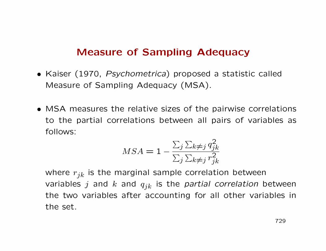
• Kaiser (1970, Psychometrica) proposed a statistic called
Measure of Sampling Adequacy (MSA).
• MSA measures the relative sizes of the pairwise correlations
to the partial correlations between all pairs of variables as
follows:
MSA = 1−∑j∑k 6=j q
2jk∑
j∑k 6=j r
2jk
where rjk is the marginal sample correlation between
variables j and k and qjk is the partial correlation between
the two variables after accounting for all other variables in
the set.
729

Measure of Sampling Adequacy
• If the r’s are relatively large and the q’s are relatively small,
MSA tends to 1. This indicates that more than two variables
are changing together as the values of the ”factor” vary
across subjects.
• Side note: If p = 3 for example, q12 is given by
q12 =r12 − r13r23√
(1− r213)(1− r2
23).
730
Measure of Sampling Adequacy
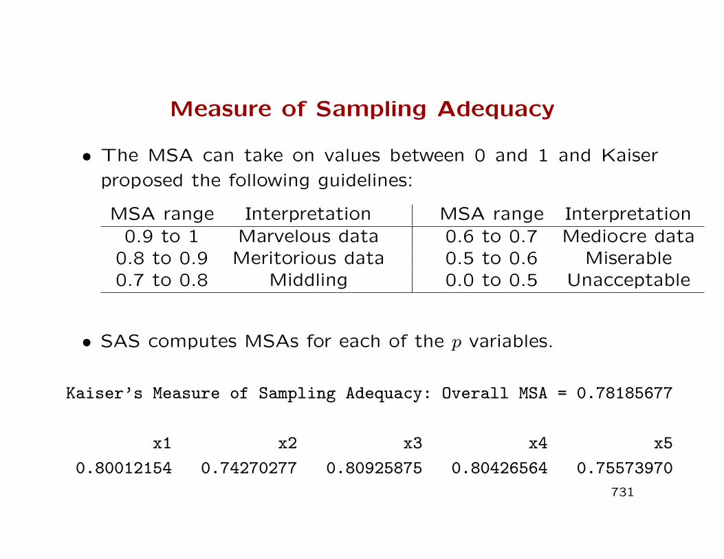
• The MSA can take on values between 0 and 1 and Kaiser
proposed the following guidelines:
MSA range Interpretation MSA range Interpretation0.9 to 1 Marvelous data 0.6 to 0.7 Mediocre data
0.8 to 0.9 Meritorious data 0.5 to 0.6 Miserable0.7 to 0.8 Middling 0.0 to 0.5 Unacceptable
• SAS computes MSAs for each of the p variables.
Kaiser’s Measure of Sampling Adequacy: Overall MSA = 0.78185677
x1 x2 x3 x4 x5
0.80012154 0.74270277 0.80925875 0.80426564 0.75573970
731

Tucker and Lewis Reliability Coefficient
• Tucker and Lewis (1973) Psychometrica, 38, pp 1-10.
• From the mle’s for m factors compute
– Lm estimates of factor loadings
– Ψm = diag(R− LmL′m)
– Gm = Ψ−1/2m diag(R− LmL′m)Ψ
−1/2m
732

Tucker and Lewis Reliability Coefficient
• gm(ij) is called the partial correlation between variables Xiand Xj controlling for the m common factors
• Sum of the squared partial correlations controlling for the m
common factors is
Fm =∑∑
i<j
g2m(ij)
• Mean square is
Mm =Fm
dfm
where dfm = 0.5[(p−m)2− p−m] are the degrees of freedom
for the likelihood ratio test of the null hypothesis that m
factors are sufficient
733

Tucker and Lewis Reliability Coefficient
• The mean square for the model with zero common factors is
M0 =
∑∑i<j r
2ij
p(p− 1)/2
• The reliability coefficient is
ρm =M0 −Mm
M0 − n−1m
where nm = (n−1)−2p+56 −2m
3 is a Bartlett correction factor.
For the weekly stock gains data SAS reports
Tucker and Lewis’s Reliability Coefficient 1.0285788
734

Cornbach’s Alpha
• A set of observed variables X = (X1, X2, . . . , Xp)′ that all
”measure” the same latent trait should all have high positive
pairwise correlations
• Define
r =
1p(p−1)/2
∑∑i<j Cov(Xi, Xj)
1p
∑pi=1
ˆV ar(Xi)=
2
p− 1
∑∑i<j Sij∑p
i=1 Sii
• Cornbach’s Alpha is
α =pr
1 + (p− 1)r=
p
p− 1
[1−
∑i V ar(Xi)
V ar(∑iXi)
]
735

Cornbach’s Alpha
• For standardized variables,∑pi=1 V ar(Xi) = p
• If ρij = 1 for all i 6= j, then
V ar(∑i
Xi) =∑i
V ar(Xi) + 2∑∑
i<j
√V ar(Xi)V ar(Xj)
=
∑i
√V ar(Xi)
2
= p2
736

Cornbach’s Alpha
• In the extreme case where all pairwise correlations are 1 wehave ∑
i V ar(Xi)
V ar(∑iXi)
=p
p2=
1
p
and
α =p
p− 1
[1−
∑i V ar(Xi)
V ar(∑iXi)
]=
p
p− 1
[1−
p
p2
]= 1
• When r = 0, then α = 0
• Be sure that the scores for all items are orientated in thesame direction so all correlations are positive
737

Factor Rotation
• As mentioned earlier, multiplying a matrix of factor loadings
by any orthogonal matrix leads to the same approximation
to the covariance (or correlation) matrix.
• This means that mathematically, it does not matter whether
we estimate the loadings as L or as L∗ = LT where T ′T =
TT ′ = I.
• The estimated residual matrix matrix also remains unchanged:
Sn − LL′ − Ψ = Sn − LTT ′L′ − Ψ = Sn − L∗L∗′− Ψ
• The specific variances ψi and therefore the communalities
also remain unchanged.
738

Factor Rotation
• Since only the loadings change by rotation, we rotate factorsto see if we can better interpret results.
• There are many choices for a rotation matrix T , and tochoose, we first establish a mathematical criterion and thensee which T can best satisfy the criterion.
• One possible objective is to have each one of the p variablesload highly on only one factor and have moderate to negli-gible loads on all other factors.
• It is not always possible to achieve this type of result.
• This can be examined with a varimax rotation
739

Varimax Rotation
• Define ˜∗ij = ˆ∗
ij/hi as the ”scaled” loading of the i-th variableon the j-th rotated factor.
• Compute the variance of the squares of the scaled loadingsfor the j-th rotated factor
1
p
p∑i=1
(˜∗ij)
2 −1
p
p∑k=1
(˜∗kj)
2
2
=1
p
p∑i=1
(˜∗ij)
4 −1
p
p∑k=1
(˜∗kj)
2
2
• The varimax procedure finds the orthogonal transformationof the loading matrix that maximizes the sum of thosevariances, summing across all m rotated factors.
• After rotation each of the p variables should load highly onat most one of the rotated factors
740

Maximum Likelihood Estimation: Stock Prices
• Varimax rotation of m = 2 factors
MLE MLE Rotated RotatedVariable factor 1 factor 2 factor 1 factor 2Allied Chem 0.68 0.19 0.60 0.38Du Pont 0.69 0.52 0.85 0.16Union Carb. 0.68 0.25 0.64 0.34Exxon 0.62 -0.07 0.36 0.51Texaco 0.79 -0.44 0.21 0.88Prop. of var. 0.485 0.113 0.334 0.264
741

Quartimax Rotation
• The varimax rotation will destroy an ”overall” factor
• The quartimax rotation try to
1. Preserve an overall factor such that each of the p variables
has a high loading on that factor
2. Create other factors such that each of the p variables has
a high loading on at most one factor
742

Quartimax Rotation
• Define ˜∗ij = ˆ∗
ij/hi as the ”scaled” loading of the i-th variable
on the j-th rotated factor.
• Compute the variance of the squares of the scaled loadings
for the i-th variable
1
m
m∑j=1
(˜∗ij)
2 −1
m
m∑k=1
(˜∗ik)
2
2
=1
m
m∑j=1
(˜∗ij)
4 −1
m
m∑k=1
(˜∗ik)2
2
• The quartimax procedure finds the orthogonal transforma-
tion of the loading matrix that maximizes the sum of those
variances, summing across all p variables.
743

Maximum Likelihood Estimation: Stock Prices
• Quartimax rotation of m = 2 factors
MLE MLE Rotated RotatedVariable factor 1 factor 2 factor 1 factor 2Allied Chem 0.68 0.19 0.71 0.05Du Pont 0.69 0.52 0.83 -0.26Union Carb. 0.68 0.25 0.72 -0.01Exxon 0.62 -0.07 0.56 0.27Texaco 0.79 -0.44 0.60 0.68Prop. of var. 0.485 0.113 0.477 0.121
744

PROMAX Transformation
• The varimax and quartimax rotations produce uncorrelated
factors
• PROMAX is a non-orthogonal (oblique) transformation that
1. is not a rotation
2. can produce correlated factors
745

PROMAX Transformation
1. First perform a varimax rotate to obtain loadings L∗
2. Construct another p×m matrix Q such that
qij = |`∗ij|k−1`∗ij for `∗ij 6= 0
= 0 for `∗ij = 0
where k > 1 is selected by trial and error, ususally k < 4.
3. Find a matrix U such that each column of L∗U is close tothe corresponding column of Q. Choose the j-th column ofU to minimize
(qj − L∗uj)′(qj − L∗uj)This yields
U = [(L∗)′(L∗)]−1(L∗)′Q
746

PROMAX Transformation
1. Rescale U so that the transformed factors have unit variance.
Compute D2 = diag[(U ′U)−1] and M = UD.
2. The PROMAX factors are obtained from
L∗F = L∗MM−1F = LPFP
• The PROMAX transformation yields factors with loadings
LP = L∗M
747
PROMAX Transformation
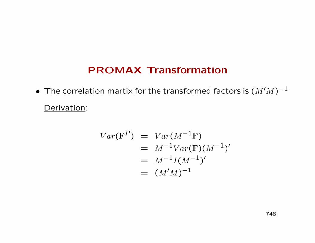
• The correlation martix for the transformed factors is (M ′M)−1
Derivation:
V ar(FP ) = V ar(M−1F)
= M−1V ar(F)(M−1)′
= M−1I(M−1)′
= (M ′M)−1
748

Maximum Likelihood Estimation: Stock Prices
• PROMAX transformation of m = 2 factors
MLE MLE PROMAX PROMAXVariable factor 1 factor 2 factor 1 factor 2Allied Chem 0.68 0.19 0.56 0.24Du Pont 0.69 0.52 0.90 -0.08Union Carb. 0.68 0.25 0.62 0.18Exxon 0.62 -0.07 0.26 0.45Texaco 0.79 -0.44 -0.02 0.92
Estimated correlation between the factors is 0.49
749

/* Varimax Rotation */
proc factor data=set1 method=ml nfactors=2
res msa mineigen=0 maxiter=75 conv=.0001
outstat=facml2 rotate=varimax reorder;
var x1-x5;
priors smc;
run;
proc factor data=set1 method=prin nfactors=3
mineigen=0 res msa maxiter=75 conv=.0001
outstat=facml3 rotate=varimax reorder;
var x1-x5;
priors smc;
run;
750

The FACTOR Procedure
Rotation Method: Varimax
Orthogonal Transformation Matrix
1 2
1 0.67223 0.74034
2 -0.74034 0.67223
Rotated Factor Pattern
Factor1 Factor2
x2 DUPONT 0.84949 0.16359
x3 UNION CARBIDE 0.64299 0.33487
x1 ALLIED CHEM 0.60126 0.37680
x5 TEXACO 0.20851 0.88333
x4 EXXON 0.36554 0.50671
751
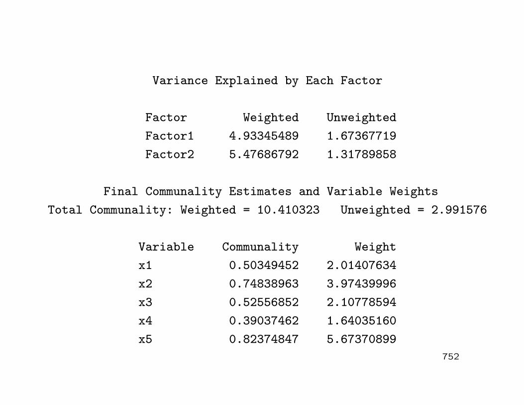
Variance Explained by Each Factor
Factor Weighted Unweighted
Factor1 4.93345489 1.67367719
Factor2 5.47686792 1.31789858
Final Communality Estimates and Variable Weights
Total Communality: Weighted = 10.410323 Unweighted = 2.991576
Variable Communality Weight
x1 0.50349452 2.01407634
x2 0.74838963 3.97439996
x3 0.52556852 2.10778594
x4 0.39037462 1.64035160
x5 0.82374847 5.67370899
752

/* Apply other rotations to the two
factor solution */
proc factor data=facml2 nfactors=2
conv=.0001 rotate=quartimax reorder;
var x1-x5;
priors smc;
run;
753

The FACTOR Procedure
Rotation Method: Quartimax
Orthogonal Transformation Matrix
1 2
1 0.88007 -0.47484
2 0.47484 0.88007
Rotated Factor Pattern
Factor1 Factor2
x2 DUPONT 0.82529 -0.25940
x3 UNION CARBIDE 0.72488 -0.01060
x1 ALLIED CHEM 0.70807 0.04611
x4 EXXON 0.56231 0.27237
x5 TEXACO 0.60294 0.67839
754

Variance Explained by Each Factor
Factor Weighted Unweighted
Factor1 7.40558481 2.38765329
Factor2 3.00473801 0.60392248
Final Communality Estimates and Variable Weights
Total Communality: Weighted = 10.410323 Unweighted = 2.991576
Variable Communality Weight
x1 0.50349452 2.01407634
x2 0.74838963 3.97439996
x3 0.52556852 2.10778594
x4 0.39037462 1.64035160
x5 0.82374847 5.67370899
755

proc factor data=facml2 nfactors=2
conv=.0001 rotate=promax reorder
score;
var x1-x5;
priors smc;
run;
756

The FACTOR Procedure
Prerotation Method: Varimax
Orthogonal Transformation Matrix
1 2
1 1.00000 -0.00000
2 0.00000 1.00000
Rotated Factor Pattern
Factor1 Factor2
x2 DUPONT 0.84949 0.16359
x3 UNION CARBIDE 0.64299 0.33487
x1 ALLIED CHEM 0.60126 0.37680
x5 TEXACO 0.20851 0.88333
x4 EXXON 0.36554 0.50671
757

Variance Explained by Each Factor
Factor Weighted Unweighted
Factor1 4.93345489 1.67367719
Factor2 5.47686792 1.31789858
Final Communality Estimates and Variable Weights
Total Communality: Weighted = 10.410323 Unweighted = 2.991576
Variable Communality Weight
x1 0.50349452 2.01407634
x2 0.74838963 3.97439996
x3 0.52556852 2.10778594
x4 0.39037462 1.64035160
x5 0.82374847 5.67370899
758

The FACTOR Procedure
Rotation Method: Promax (power = 3)
Target Matrix for Procrustean Transformation
Factor1 Factor2
x2 DUPONT 1.00000 0.00733
x3 UNION CARBIDE 0.73686 0.10691
x1 ALLIED CHEM 0.64258 0.16242
x5 TEXACO 0.01281 1.00000
x4 EXXON 0.21150 0.57860
Procrustean Transformation Matrix
1 2
1 1.24806851 -0.3302485
2 -0.3149179 1.20534878
759

Normalized Oblique Transformation Matrix
1 2
1 1.11385973 -0.3035593
2 -0.2810538 1.10793795
Inter-Factor Correlations
Factor1 Factor2
Factor1 1.00000 0.49218
Factor2 0.49218 1.00000
760

Rotated Factor Pattern (Standardized Regression Coefficients)
Factor1 Factor2
x2 DUPONT 0.90023 -0.07663
x3 UNION CARBIDE 0.62208 0.17583
x1 ALLIED CHEM 0.56382 0.23495
x5 TEXACO -0.01601 0.91538
x4 EXXON 0.26475 0.45044
761

Reference Structure (Semipartial Correlations)
Factor1 Factor2
x2 DUPONT 0.78365 -0.06670
x3 UNION CARBIDE 0.54152 0.15306
x1 ALLIED CHEM 0.49081 0.20452
x5 TEXACO -0.01394 0.79683
x4 EXXON 0.23046 0.39211
Variance Explained by Each Factor Eliminating Other Factors
Factor Weighted Unweighted
Factor1 3.63219833 1.20154790
Factor2 4.00599560 0.85839588
762

Factor Structure (Correlations)
Factor1 Factor2
x2 DUPONT 0.86252 0.36645
x3 UNION CARBIDE 0.70862 0.48200
x1 ALLIED CHEM 0.67946 0.51245
x5 TEXACO 0.43452 0.90750
x4 EXXON 0.48644 0.58074
Variance Explained by Each Factor Ignoring Other Factors
Factor Weighted Unweighted
Factor1 6.40432722 2.13317989
Factor2 6.77812448 1.79002787
763

Final Communality Estimates and Variable Weights
Total Communality: Weighted = 10.410323 Unweighted = 2.991576
Variable Communality Weight
x1 0.50349452 2.01407634
x2 0.74838963 3.97439996
x3 0.52556852 2.10778594
x4 0.39037462 1.64035160
x5 0.82374847 5.67370899
764

Scoring Coefficients Estimated by Regression
Squared Multiple Correlations of the Variables with Each Factor
Factor1 Factor2
0.83601404 0.84825886
Standardized Scoring Coefficients
Factor1 Factor2
x2 DUPONT 0.58435 -0.01834
x3 UNION CARBIDE 0.21791 0.06645
x1 ALLIED CHEM 0.18991 0.08065
x5 TEXACO 0.02557 0.78737
x4 EXXON 0.07697 0.11550
765

R code posted in stocks.R
# Compute maximun likelihood estimates for factors
stocks.fac <- factanal(stocks, factors=2,
method=’mle’, scale=T, center=T)
stocks.fac
Call: factanal(x = stocks, factors = 2, method = "mle",
scale = T, center = T)
Uniquenesses:
x1 x2 x3 x4 x5
0.497 0.252 0.474 0.610 0.176
766

Loadings:
Factor1 Factor2
x1 0.601 0.378
x2 0.849 0.165
x3 0.643 0.336
x4 0.365 0.507
x5 0.207 0.884
Factor1 Factor2
SS loadings 1.671 1.321
Proportion Var 0.334 0.264
Cumulative Var 0.334 0.598
Test of the hypothesis that 2 factors are sufficient.
The chi square statistic is 0.58 on 1 degree of freedom.
The p-value is 0.448
767

# Apply the Varimax rotation (this was the default)
stocks.fac <- factanal(stocks, factors=2, rotation="varimax",
method="mle", scores="regression")
stocks.fac
Call: factanal(x = stocks, factors = 2, scores = "regression",
rotation = "varimax", method = "mle")
Uniquenesses:
x1 x2 x3 x4 x5
0.497 0.252 0.474 0.610 0.176
768

Loadings:
Factor1 Factor2
x1 0.601 0.378
x2 0.849 0.165
x3 0.643 0.336
x4 0.365 0.507
x5 0.207 0.884
Factor1 Factor2
SS loadings 1.671 1.321
Proportion Var 0.334 0.264
Cumulative Var 0.334 0.598
Test of the hypothesis that 2 factors are sufficient.
The chi square statistic is 0.58 on 1 degree of freedom.
The p-value is 0.448
769

# Compute the residual matrix
pred<-stocks.fac$loadings%*%t(stocks.fac$loadings)
+diag(stocks.fac$uniqueness)
resid <- s.cor - pred
resid
x1 x2 x3 x4 x5
x1 -8.4905e-07 4.5256e-03 -4.1267e-03 -2.3991e-02 3.9726e-03
x2 4.5256e-03 1.8641e-07 -2.6074e-03 -3.8942e-03 3.2772e-04
x3 -4.1267e-03 -2.6074e-03 7.4009e-08 3.1384e-02 -4.2413e-03
x4 -2.3991e-02 -3.8942e-03 3.1384e-02 -1.7985e-07 -2.8193e-04
x5 3.9726e-03 3.2772e-04 -4.2413e-03 -2.8193e-04 2.7257e-08
770

# List factor scores
stocks.fac$scores
Factor1 Factor2
1 -0.05976839 0.02677225
2 -1.22226529 1.44753390
3 1.62739601 2.47578797
. . .
. . .
99 0.71440818 -0.02122186
100 -0.59289113 0.34344739
771

# You could use the following code in Splus to apply
# the quartimax rotation, but this is not available in R
#
# stocks.fac <- factanal(stocks, factors=2, rotation="quartimax",
# method="mle", scores="regression")
# stocks.fac
# Apply the Promax rotation
promax(stocks.fac$loadings, m=3)
772

Loadings:
Factor1 Factor2
x1 0.570 0.195
x2 0.965 -0.174
x3 0.639 0.125
x4 0.226 0.456
x5 -0.128 0.984
Factor1 Factor2
SS loadings 1.732 1.260
Proportion Var 0.346 0.252
Cumulative Var 0.346 0.598
$rotmat
[,1] [,2]
[1,] 1.2200900 -0.4410072
[2,] -0.4315772 1.2167132
773

# You could try to apply the promax rotation with the
# factanal function. It selects the power as m=4
>
> stocks.fac <- factanal(stocks, factors=2, rotation="promax",
+ method="mle", scores="regression")
>
> stocks.fac
Call:
factanal(x = stocks, factors = 2, scores = "regression", rotation = "promax", method = "mle")
Uniquenesses:
x1 x2 x3 x4 x5
0.497 0.252 0.474 0.610 0.176
774

Loadings:
Factor1 Factor2
x1 0.576 0.175
x2 1.011 -0.232
x3 0.653
x4 0.202 0.466
x5 -0.202 1.037
Factor1 Factor2
SS loadings 1.863 1.387
Proportion Var 0.373 0.277
Cumulative Var 0.373 0.650
Test of the hypothesis that 2 factors are sufficient.
The chi square statistic is 0.58 on 1 degree of freedom.
The p-value is 0.448
775

Example: Test Scores
• The sample correlation between p = 6 test scores collected
from n = 220 students is given below:
R =
1.0 0.439 0.410 0.288 0.329 0.2481.0 0.351 0.354 0.320 0.329
1.0 0.164 0.190 0.1811.0 0.595 0.470
1.0 0.4641.0
.
• An m = 2 factor model was fitted to this correlation matrix
using ML.
776
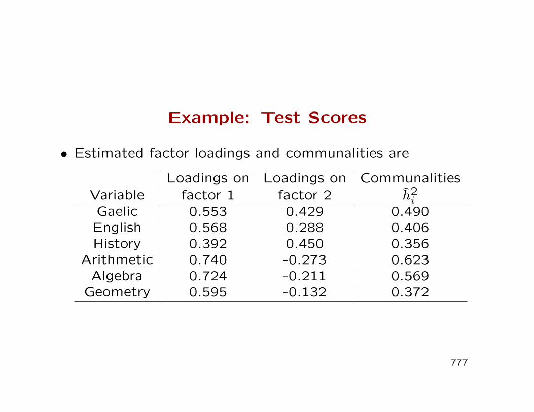
Example: Test Scores
• Estimated factor loadings and communalities are
Loadings on Loadings on CommunalitiesVariable factor 1 factor 2 h2
iGaelic 0.553 0.429 0.490
English 0.568 0.288 0.406History 0.392 0.450 0.356
Arithmetic 0.740 -0.273 0.623Algebra 0.724 -0.211 0.569
Geometry 0.595 -0.132 0.372
777

Example: Test Scores
• All variables load highly on the first factor. We call that a’general intelligence’ factor.
• Half of the loadings are positive and half are negative on thesecond factor. The positive loadings correspond to the ’ver-bal’ scores and the negative correspond to the ’math’ scores.
• Correlations between scores on verbal tests and math teststend to be lower than correlations among scores on mathtests or correlations among scores on verbal tests, so this isa ’math versus verbal’ factor.
• We plot the six loadings for each factor (ˆi1, ˆi2) on the orig-inal coordinate system and also on a rotated set of coor-dinates chosen so that one axis goes through the loadings(ˆ41, ˆ42) of the fourth variable on the two factors.
778

Factor Rotation for Test Scores
779

Varimax Rotation for Test Scores
• Loadings for rotated factors using the varimax criterion are
as follows:
Loadings on Loadings on CommunalitiesVariable F ∗1 F ∗2 h2
iGaelic 0.232 0.660 0.490
English 0.321 0.551 0.406History 0.085 0.591 0.356
Arithmetic 0.770 0.173 0.623Algebra 0.723 0.215 0.569
Geometry 0.572 0.213 0.372
• F ∗1 is primarily a ’mathematics ability factor’ and F ∗2 is a
’verbal ability factor’.
780

PROMAX Rotation for Test Scores
• F ∗1 is more clearly a ’mathematics ability factor’ and F ∗2 is a’verbal ability factor’.
Loadings on Loadings on CommunalitiesVariable F ∗1 F ∗2 h2
iGaelic 0.059 -0.668 0.490
English 0.191 0.519 0.406History -0.084 0.635 0.356
Arithmetic 0.809 0.041 0.623Algebra 0.743 0.021 0.569
Geometry 0.575 0.064 0.372
• These factors have correlation 0.505
• Code is posted as Lawley.sas and Lawley.R
781

Factor Scores
• Sometimes, we require estimates of the factor values for eachrespondent in the sample.
• For j = 1, ..., n, the estimated m−dimensional vector of factorscores is
fj = estimate of values fj attained by Fj.
• To estimate fj we act as if L (or L) and Ψ (or Ψ) aretrue values.
• Recall the model
(Xj − µ) = LFj + εj.
782

Weighted Least Squares for Factor Scores
• From the model above, we can try to minimize the weightedsum of squares
p∑i=1
ε2iψi
= ε′Ψ−1ε = (x− µ− Lf)′Ψ−1(x− µ− Lf).
• The weighted least squares solution is
f = (L′Ψ−1L)−1L′Ψ−1(x− µ).
• Substituting the MLEs L, Ψ, x in place of the true values, wehave
fj = (L′Ψ−1L)−1L′Ψ−1(xj − x).
783

Weighted Least Squares for Factor Scores
• When factor loadings are estimated with the PC method,ordinary least squares is sometimes used to get the factorscores. In this case
fj = (L′L)−1L′(xj − x).
• Implicitly, this assumes that the ψi are equal or almost equal.
• Since L = [√λ1e1
√λ2e2 ...
√λmem], we find that
fj =
λ−1/21 e′1(xj − x)
λ−1/22 e′2(xj − x)
...
λ−1/2m e′m(xj − x)
.784

Weighted Least Squares for Factor Scores
• Note that the factor scores estimated from the principal
component solution are nothing more than the scores for
the first m principal components scaled by λ−1/2i ,
for i = 1, ...,m.
• The estimated factor scores have zero mean and zero
covariances.
785

Regression Method for Factor Scores
• We again start from the model (X − µ) = LF + ε.
• If the F, ε are normally distributed, we note that(X − µF
)∼ Np+m(0,Σ∗),
with
Σ∗(p+m)×(p+m) =
[Σ = LL′+ Ψ L
L′ I
].
• The conditional distribution of F given X = x is thereforealso normal, with
E(F |x) = L′Σ−1(x− µ) = L′(LL′+ Ψ)−1(x− µ)
Cov(F |x) = I − L′Σ−1L = I − L′(LL′+ Ψ)−1L.
786

Regression Method for Factor Scores
• An estimate of fj is obtained by substituting estimates forthe unknown quantities in the expression above, so that
fj = E(Fj|xj) = L′(LL′+ Ψ)−1(xj − x).
• Sometimes, to reduce the errors that may be introduced ifthe number of factors m is not quite appropriate, S is usedin place of (LL′+ Ψ) in the expression for fj.
• If loadings are rotated using T , the relationship between theresulting factor scores and the factor scores arising from un-rotated loadings is
f∗j = T fj.
787

Factor Scores for the Stock Price Data
• We estimated the value of the two factor scores for each of
the 100 observations in the stock price example. Note that
scatter plot shows approximate mean 0 and variance 1 and
approximate bivariate normality.
788


Heywood Cases and Other Potential Problems
• When loadings are estimated iteratively (as in the Principal
Factor or ML methods) some problems may arise:
– Some of the estimated eigenvalues of R−Ψ may become
negative.
– Some of the communalities may become larger than one.
• Since communalities estimate variances, they must be
positive. If any communality exceeds 1.0, the variance
of the corresponding specific factor is negative.
789

Heywood Cases and Other Potential Problems
• When can these things happen?
1. When we start with bad prior communality estimates for
iterating.
2. When there are too many common factors.
3. When we do not have enough data to obtain stable
estimates.
4. When the common factor model is just not appropriate
for the data.
• These problems can occur even in seemingly ’good’ datasets
(see example below) and create serious problems when we
try to interpret results.
790

Heywood Cases and Other Potential Problems
• When a final communality estimate equals 1, we refer to
this as a Heywood case (a solution on the boundary of the
parameter space).
• When a final communality estimate exceeds 1, we have an
Ultra Heywood case.
• An Ultra Heywood case implies that unique factor has
negative variance, a huge red flag that something is
wrong and that results from the factor analysis are invalid.
791

Heywood Cases and Other Potential Problems
• There is some concern about the validity of results in
Heywood cases (boundary solutions where the factors
account for all of the variation in at least one trait).
It is difficult to interpret results (for example, how
can a confidence interval be constructed for a parameter
at the boundary?)
• Large sample results may not be valid for Heywood cases,
in particular large sample chi-square approximations for a
likelihood ratio tests (e.g. test for the number of factors).
792

Heywood Cases and Other Potential Problems
• When iterative algorithms in SAS fail to converge, we caninclude a heywood or an ultra heywood option in the procfactor statement.
– The heywood option fixes to 1 any communality thatgoes above 1 and continues iterating on the rest.
– The ultraheywood option continues iterating on allvariables, regardless of the size of the communalities,hoping that the soultion eventually comes back insidethe parameter space (this rarely happens).
• When factor loadings are estimated using the principalcomponents method, none of these problems arise (assumingthat R is of full column rank).
793

Example: track records for men and women
• Use maximum liklelihood estimation to fit factor models tostandardized observations on national track records for menand women in n = 54 countries (Table 8.6 and Table 1.9).
• The dataset for women includes seven variables x1, ..., x7 thatcorrespond to national records on 100m, 200m, 400m, 800m,1500m, 3000m and marathon races.
• The dataset for men includes eight variables x1, ..., x8 thatcorrespond to national records on 100m, 200m, 400m, 800m,1500m, 5000m, 10000m and marathon races.
• The first three times are in seconds and the remaining timesare in minutes.
794

Example: track records for men and women
• First examine scatterplots and correlation matrices.
• Test for the appropriate number of factors using
likelihood ratio tests.
• The HEYWOOD option is needed in the FACTOR procedure
in SAS for the three factor model for both men and women.
• SAS code to carry out these analyses is posted as records.sas
and R code is posted as records.R on the course web page.
795

Example: track records for men
• The scatter plot matrix reveals a couple of extreme countrieswith slow times but they conform to the correlation pattern.All relationships are approximately straight line relationships.
• Results indicate that the two factor model may be reasonable(p-value=.0173). MLE’s for the factor loadings are inside theparameter space and the two rotated (varimax) factors areeasy to interpret.
• Since the MLE for the three factor solution is on theboundary of the parameter space, we are not justified inusing a large sample chi-square approximation for thelikelihood ratio test and the reported p-value (.2264) isunreliabale.
796

100m
−2 1 3
●
●
●●●
●●
●●●
●
●●●●●
●●
●
●
●
●
●●
●●
●●
●●
●
●●
●●
●
●●●
●●
●●
●●
●
●
●●●
●●
●
●
●
●
●●●
●●
●●●
●
●●●
●●
●●
●
●
●
●
●●
●●
●●
● ●
●
●●
●●
●
●●●
●●
●●
●●
●
●
●●●
●●●
●
−1 1 3
●
●
●●●
●●
●●●
●
●●●
●●
●●
●
●
●
●
●●
●●
● ●
● ●
●
●●●
●
●
●●●
●●
●●
●●
●
●
●●●
●●
●
●
●
●
●●●
●●
●●●
●
●●●
●●
●●
●
●
●
●
●●
●●
●●
● ●
●
●●
●●
●
●●●
●●
●●
●●
●
●
● ●●
●●
●
●
−1 1 3
●
●
●●●
●●
●●●
●
●●●
●●
●●
●
●
●
●
●●
●●
●●
● ●
●
●●●
●
●
●●●
●●
●●
●●
●
●
●●●
●●
●
●
●
●
●●●
●●
●●●
●
●●●
●●
●●
●
●
●
●
●●
●●
●●
● ●
●
●●●
●
●
●●●
●●
●●
●●
●
●
●●●
●●
●
●
−1 1 3
−2
02
●
●
●●●
●●
●●●
●
●●●
●●
●●
●
●
●
●
●●
●●
●●
●●
●
●●
●●
●
●●●
●●
●●
●●
●
●
●●●
●●
●
●
−2
13
●●
●●●
●● ●
●●
●
●●●●●
●●● ●
●
●
●●
●●
●●
●●
●●●
●●
●
●●●
●●
●●
●
●
●
●
●●●●●●
●
200m●
●●
●●●● ●●●
●
●●●●●
●●● ●
●
●
●●
●●
●●
● ●
●●●
●●
●
●●●
●●
● ●
●
●
●
●
●●●●●●
●
●●
●● ●
●●●
●●
●
●●● ●●
●●● ●
●
●
●●
●●
●●
● ●
●●●
●●
●
●●
●
●●
●●
●
●
●
●
●●●●●
●
●
●●●● ●●
● ●●
●
●
●●● ●●
●●● ●
●
●
●●
●●
●●
● ●
●●●
●●
●
●●
●
●●
●●
●
●
●
●
● ●●●●
●
●
●●
●● ●
●●●●●
●
●●● ●●
●●●●
●
●
●●
●●
●●
● ●
●●●
●●
●
●●●
●●
●●
●
●
●
●
●●●●●
●
●
●●●
● ●●
●●●●
●
●●● ●●
●●●●
●
●
●●
●●
●●
● ●
●●●
●●
●
●●●
●●
●●
●
●
●
●
●●●●●
●
●
●●
●● ●●
●●●●
●
●●● ●●
●●●●
●
●
●●
●●
●●●●
●● ●
●●
●
●●●
●●
●●
●
●
●
●
●●●●●
●
●
●
●
●●●
●●●●
●
●
●●●
●●
●●●●
●
● ●●
●●
●●●●
●●
●
●●
●
●●●●
●●
● ●●
●
●
●●●
●●
●
●
●
●
●●●
●●●
●●
●
●●●●
●●●●
●
●
● ●●
●●
●●●●
●●
●
●●
●
●●●●
●●
● ●●
●
●
●●●
●●
●
●
400m●
●
●● ●
● ●●●
●
●
●●●
●●
●●●●
●
●●●
●●
● ●●
●
●●
●
●●
●
●●●●●
●
●●●
●
●
●●
●
●●
●
●
●
●
●● ●●●
●●
●
●
●●●
●●
●●●●
●
●●●
●●
●●●
●
●●
●
●●
●
●●●●
●●
●●●
●
●
●●
●
●●
●
●
●
●
●● ●
●●●●●
●
●●●
●●
●●●●
●
●●●
●●
●●●
●
●●
●
●●
●
●●●●
●●
●●●
●
●
●●
●
●●
●
●
●
●
●● ●
●●●●●
●
●●●
●●●●●
●
●
●●●
●●
●●●
●
●●
●
●●
●
●●●●
●●
●●●
●
●
●●●
●●
●
● −2
13
●
●
●● ●●●
●●●
●
●●●
●●
●●●●
●
●●●
●●
●●●●
●●
●
●●
●
●●●●
●●
● ●●
●
●
●●●
●●
●
●
−1
13
●●
●
●
●
●
● ●●●
●
●
●
●
●
●●●
●
●
●
● ●
●
●
●
●
●
●
●
●
●●●
●●
●●●
● ●
●● ●
●
●
●
●●
●
●●
●
●
●●
●
●
●
●
●●●
●
●
●
●
●
●
●●●
●
●
●
● ●
●
●
●
●
●
●
●
●
●●●
●●
●●●
●●
●● ●
●
●
●
●●
●
●●
●
●
●●
●
●
●
●
● ●●●
●
●
●
●
●
●●●●
●
●
●●
●
●
●
●
●
●
●
●
●●●
●●
●●●
●●
●●●
●
●
●
●●
●
●●●
●
800m●
●●
●
●
●
● ●●●
●
●
●
●
●
●●●●
●
●
●●
●
●
●
●
●
●
●
●
●●●
●●
●●●
●●
●●●
●
●
●
●●
●
●●
●
●
●●
●
●
●
●
●●●●
●
●
●
●
●
●●●●
●
●
●●
●
●
●
●
●
●
●
●
●●●●●
●●●
●●
●●●
●
●
●
●●
●
●●
●
●
●●●
●
●
●
●●●●
●
●
●
●
●
●●●●
●
●
●●
●
●
●
●
●
●
●
●
●●●●●
●●●
●●
●●●
●
●
●
●●
●
●●
●
●
●●
●
●
●
●
●●●●
●
●
●
●
●
●●●●
●
●
●●
●
●
●
●
●
●
●
●
●●●
●●
●●●
●●
●● ●
●
●
●
●●
●
●●
●
●
●
● ●●
●
●●●●
●
●
●
●●
●●
●●●●
●
● ●
●
●
●
●●
●
●
●●
●●
●
●
●●●
●
●
●●
●●
●
●
●
●●
●●
●
●
●
● ●●
●
●●●●
●
●
●
●●
●●
●●●●
●
● ●
●
●
●
●●
●
●
●●●
●
●
●
●●●
●
●
●●
●●
●
●
●
●●
●●
●
●
●
● ●●
●
●●●●●
●
●
●●
●●
●●●●
●
●●
●
●
●
●●
●
●
●●
●●
●
●
●●●
●
●
●●
●●
●
●
●
●●
●●
●
●
●
●●●
●
● ●●●
●
●
●
●●
●●
●●●●
●
●●
●
●
●
●●
●
●
●●
●●
●
●
●●●
●
●
●●●●
●
●
●
●●
●●
●
●
1500m●
●●●
●
●●●●●
●
●
●●
●●
●●●●
●
●●
●
●
●
●●
●
●
●●
●●
●
●
●●●
●
●
●●●●
●
●
●
●●
●●
●
●
●
●●●
●
●●●●●
●
●
●●
●●
●●●●
●
●●
●
●
●
●●
●
●
●●
●●
●
●
●●●
●
●
●●●●
●
●
●
●●
●●
●
● −1
13
●
●●●
●
●●●●●
●
●
●●
●●
●●●●
●
●●
●
●
●
●●
●
●
●●
●●
●
●
●●●
●
●
●●
●●
●
●
●
●●
●●
●
●
−1
13
●●
●●
●
●● ●●●
●
●●●
●
●●●●
●●
● ●
●
●●
●●●
● ●●
●●
●
●
●●●
●
●
●● ●●
●
●
●●●
●●
●●
●●
●●
●
●●●● ●
●
●●●
●
●●●●
●●
● ●
●
●●
●●●
● ●●●●
●
●
●●●
●
●
●● ●●
●
●
●●●
●●
●●
●●
●●
●
●● ●●●
●
●●●
●
●●●●
●●
●●
●
●●
●●●
● ●●
●●
●
●
●●●
●
●
● ●●●
●
●
●●●
●●
●●
●●
●●
●
● ●●●●
●
●●●
●
●●●●
●●
●●
●
●●
● ●●
● ●●
●●
●
●
●●●
●
●
●●●●
●
●
●●●
●●
●●
●●●●
●
●● ●● ●
●
●●●
●
●●●●
●●
●●
●
●●
●●●
● ●●
●●
●
●
●●●
●
●
●●●●
●
●
● ●●
●●
●●
5000m●●●
●
●
●●●●●
●
●●●
●
●●●●
●●
●●
●
●●
●●●
●●●●●
●
●
●●●
●
●
●●●●
●
●
●●●
●●
●●
●●
●●
●
●●●●●
●
●●●
●
●●●●
●●●●
●
●●
●●●
●●●●●
●
●
●●●
●
●
●● ●●
●
●
●●●
●●
●●
●● ●●
●
●● ●●●
●
●●●
●
●●●●●
●●
●●
●●
●●●
● ●●●●
●
●
●●●
●
●●
● ●●
●
●
●●●
●●●
● ●● ●●
●
●●●● ●
●
●●●
●
●●●●●
●●
●●
●●
●●●
● ●●●●
●
●
●●●
●
●●● ●●
●
●
●●●
●●●
● ●● ●●
●
●● ●●●
●
●●●
●
●●●●●
●●●
●
●●
●●●
● ●●●●
●
●
●●●
●
●●
●●●
●
●
●●●
●●●
● ●●●●
●
● ●●●●
●
●●●
●
●●●●●
●●●
●
●●
● ●●
● ●●●●
●
●
●●●
●
●●
●●●
●
●
●●●
●●●
● ●●●●
●
●● ●● ●
●
●●●
●
●●●●●
●●●
●
●●
●●●
● ●●●●
●
●
●●●
●
●●
●●●
●
●
●●●
●●●
● ●●●●
●
●●●●●
●
●●●
●
●●●●●
●●●
●
●●
●●●
●●●●●
●
●
●●●
●
●●
●●●
●
●
●●●
●●●
●
10000m
−1
13
●●●●
●
●●●●●
●
●●●
●
●●●●●●●●
●
●●
●●●
●●●●●
●
●
●●●
●
●●
● ●●
●
●
●●●
●●●
●
−2 0 2
−1
13
●●●●
●
●● ●
●●
●
●●●
●
●●●●
● ●● ●●
●●
●● ●●●
●
●●
●
●
●●●
●
●
●●●
●
●
●
●●●
●●
●●
●●●
●
●
●●●● ●
●
●●●
●
●●●●
● ●● ●●
●●
●● ●●●
●
●●
●
●
●●●
●
●
●●●
●
●
●
●●●
●●
●●
−2 1 3
●●●
●
●
●● ●●●
●
●●●
●
●●●●
● ●●●●
●●
●●● ● ●●
●●
●
●
●●●
●
●
● ●●
●
●
●
●●●
●●
●●
●●●
●
●
●●●●●
●
●●●
●
●●●●
● ●●●●
●●
● ●● ● ●●
●●
●
●
●●●
●
●
●●●
●
●
●
●●●
●●
●●
−1 1 3
●●●●
●
●● ●
● ●
●
●●●
●
●●●●
● ●●●●
●●
●●● ● ●●
●●
●
●
●●●
●
●
●●●
●
●
●
●●●
●●
●●
●●●
●
●
●●●●●
●
●●●
●
●●●●
● ●●●●
●●
●●● ●●●
●●
●
●
●●●
●
●
●●●●
●
●
●●●
●●
●●
−1 1 3
●●●
●
●
●●●●●
●
●●●
●
●●●●
● ●●●●
●●
●●● ●●●
●●
●
●
●●●
●
●
●●●●
●
●
●●●
●●
●●
marathon
797

Example: track records for men
Varimax Varimax Promax PromaxRace Factor 1 Factor 2 Factor 1 Factor 2 h2
i100m 0.402 0.839 0.097 0.868 0.865200m 0.409 0.892 0.068 0.933 0.963400m 0.515 0.711 0.300 0.643 0.772800m 0.671 0.581 0.568 0.393 0.787
1500m 0.748 0.554 0.682 0.316 0.8665000m 0.886 0.450 0.915 0.109 0.987
10000m 0.900 0.424 0.946 0.069 0.989Marathon 0.865 0.402 0.910 0.063 0.912
• The Promax factors have correlation 0.697
• There is a distance race factor and a sprint factor
798
Example: track records for women
• The two factor model does not appear to fit for women
(p-value<.0001).
• The algorithm for fitting the three-factor model needed the
Heywood option to converge to a boundary solution. (The
reported p-value of 0.0295 for the likelihood ratio test is un-
reliable.)
• Two varimax rotated factors have a similar interpretation to
the rotated factors for men, but the marathon does not load
so highly on the distance factor
799

Example: track records for women
• Three varimax rotated factors allow for a sprint factor, a
1500m and 3000m factor, and a third factor for which the
800m and the marathon have relatively high loadings.
• A four factor solution does not split up the loadings on the
third factor for the 800m and marathon races.
800

100m
−2 0 2
●
●●●
●
●●
●
●
●
●
●
●
●●
●
●●
●●
●
●●
●●●
●●●
●
●●●
●
●
●
●●●
●
●
●
●●
●
●●
●●●
●●●
●
●
● ●●
●
●●
●
●
●
●
●
●
●●
●
●●
●●
●
●●
●●●
●●●
●
●●●
●
●
●
●●●
●
●
●
●●
●
●●
● ●●
●●●
●
−1 1 3
●
●●●
●
●●
●
●
●
●
●
●
●●
●
●●
●●
●
●●
●● ●
●●
●●
● ●●
●
●
●
●● ●
●
●
●
●●
●
●●
●●●
●●●
●
●
●●●
●
●●
●
●
●
●
●
●
●●
●
●●
●●
●
●●
●● ●
●●
●●
●●●
●
●
●
●●●
●
●
●
●●
●
●●
●●●
●●●
●
−1 1 3 5
●
●●●
●
●●
●
●
●
●
●
●
●●
●
●●
●●
●
●●
●● ●
●●
●●
●●●●
●
●
●●●
●
●
●
●●
●
●●
●●●
●●●
● −2
02
●
● ●●
●
●●
●
●
●
●
●
●
●●
●
●●
●●
●
●●●● ●
●●●
●
●●●●
●
●
●●●
●
●
●
●●
●
●●
●●●
●●●
●−
20
2
●
●●●
●●●
●
●
●
●
●
●
●●
●●●
●●
●
●
●
●●●
●
● ●●
●
●●
●
●●
●●●
●
●
●
●●
●
●
●
●●●●
●●
●
200m●
●●●
●●●
●
●
●
●
●
●
●●
●●
●●
●
●
●
●
●●●
●
●●●
●
●●
●
●●
●●●
●
●
●
●●
●
●
●
●●●
●
●●
●
●
●●●
●●●
●
●
●
●
●
●
●●
●●
●●
●
●
●
●
●●●
●
●●●
●
●●
●
●●
●● ●
●
●
●
●●●
●
●
●●●
●
●●
●
●
●●●
●●●
●
●
●
●
●
●
●●
●●
●●
●
●
●
●
●● ●●
●●●
●
●●
●
●●
●●●
●
●
●
●●●
●
●
●●●
●
●●
●
●
●●●
●●●
●
●
●
●
●
●
●●
●●●●
●
●
●
●
●● ●●
●●●
●
●●●
●●
●●●
●
●
●
●●●
●
●
●●●
●
●●
●
●
●●●
●●●
●
●
●
●
●
●
●●
●●
●●
●
●
●
●
●● ●●
●●●
●
●●●
●●
●●●
●
●
●
●●●
●
●
●●●
●
●●
●
●
●
●●
●
●●
●
● ●
●
●
●
●●
●●●
●●
●
●
●
●●●● ● ●
●
●●
●
●
●
●● ●
●
●●
●
●
●●
●●
●
●●●●●
●
●
●
●●
●
●●
●
● ●
●
●
●
● ●
●●●●
●
●
●
●
●●●● ●●
●
●●
●
●
●
●●●
●
●●
●
●
●●
●●
●
●●● ●●
●
400m●
●
●●
●
●●
●
● ●
●
●
●
● ●
●●●●
●
●
●
●
●●●● ●●
●
● ●
●
●
●
●●●
●
●●
●
●
●●
●●
●
●●●●●
●
●
●
●●
●
●●
●
● ●
●
●
●
● ●
●●●
●●
●
●
●
●●●● ●●
●
●●
●
●
●
●●●
●
●●
●
●
●●
●●
●
●●●●●
●
●
●
●●
●
●●
●
● ●
●
●
●
● ●
●●●
●●
●
●
●
●●●●●●
●
●●
●
●
●
●●●●
●●
●
●
●●
●●
●
●●●●●
● −1
13
●
●
●●
●
●●
●
● ●
●
●
●
● ●
●●●
●●
●
●
●
●●●●●●
●
●●
●
●
●
●●●●
●●
●
●
●●
●●
●
●●●●●
●
−1
13
●
●●●
●
●●●
●
●
●
●
●
●
●
●
●● ●
●
●
●
●
●●
●
●●
●
●
●
●●
●● ●
●●
●
●
●
●●
●●
●
●
●●●
●●●
●
●
●●
●
●
●●●
●
●
●
●
●
●
●
●
●●●
●
●
●
●
●●
●
●●●
●
●
●●
●● ●
●●
●
●
●
●●
●●
●
●
●●●
● ●●
●
●
●●●
●
●●●
●
●
●
●
●
●
●
●
●● ●
●
●
●
●
●●
●
●●●
●
●
●●
●● ●
●●
●
●
●
●●
●●
●
●
●●●
●●●
●
800m ●
●●●
●
●●●
●
●
●
●
●
●
●
●
●●●
●
●
●
●
●●
●
●●
●
●
●
●●
●●●
●●
●
●
●
●●
●●
●
●
●●●
●●●
●
●
●●●
●
●●●
●
●
●
●
●
●
●
●
●●●
●
●
●
●
●●
●
●●
●
●
●
●●
●●●
●●
●
●
●
●●
●●
●
●
●●●
●●●
●
●
●●
●
●
●●●
●
●
●
●
●
●
●
●
●●●
●
●
●
●
●●
●
●●●
●
●
●●
●● ●
●●
●
●
●
●●
●●
●
●
●●●
●●●
●
●
●●●●
●●
●
●
●
●
●
●●
●
●●● ●●
●
●
●
●●
●
●●
●
● ●●● ●
● ●● ●
●
●●
● ●●●
●
●
●●●
●●
●●
●
●●●●
●●
●
●
●
●
●
●●
●
●●●●●
●
●
●
●●
●
●●●
● ●●●●
● ●●●
●
●●
● ●●●
●
●
●●●
● ●
●●
●
● ●●●
●●
●
●
●
●
●
●●
●
●●● ●●
●
●
●
●●
●
●●●
● ●●● ●
● ●●●●
●●
● ●●●
●
●
● ●●
●●
●●
●
●●●●
●●
●
●
●
●
●
●●
●
●●●●●
●
●
●
●●
●
●●
●
●●● ●●
●●●●
●
●●
●●●●
●
●
●●●
●●
●●
1500m●
●●●●
●●
●
●
●
●
●
●●
●
●●●●●
●
●
●
●●
●
●●
●
●●●●●
●●●●●
●●
●●●●
●
●
●●●
●●
●● −1
13
●
● ●●●
●●
●
●
●
●
●
●●
●
●●●●●
●
●
●
●●
●
●●●
●●● ●●
● ●●●●
●●
●●●●
●
●
●●●
●●
●●
−1
13
5
●●●●
●
●●
●
●
●
●
●
● ●
●
●●● ●●
●
●
●●
●
●
● ●●
● ●●● ●
● ●● ●●
●●
● ●●●
●
●
●●●
●●
●●
●●●●
●
●●
●
●
●
●
●
● ●
●
●●●●●
●
●
●●
●
●
● ●●
● ●●●●● ●
●●●
●●
● ●●●
●
●
●●●
●●
●●
●● ●●
●
●●
●
●
●
●
●
● ●
●
●●● ●●
●
●
●●
●
●
●●●● ●●
● ●● ●
●●●
●●
● ●●●
●
●
●●●
●●
●●
●●●●
●
●●
●
●
●
●
●
● ●
●
●●●●●
●
●
●●
●
●
● ●●
●● ● ●●●●
●● ●
●●
●●●●
●
●
●●●
●●
●●
●●●●
●
●●
●
●
●
●
●
●●
●
●●●●●
●
●
●●
●
●
● ●●
●●●●●●●
●●●
●●
●●●●
●
●
●●●
●●
●●
3000m●
● ●●
●
●●
●
●
●
●
●
●●
●
●●●●●
●
●
●●
●
●
●●●
●●●●●
● ●●●●
●●
●●●●
●
●
●●●
●●
●●
−2 0 2
●●●●
●
●● ●
●
●
●
●
● ●
●
●●●
●
●
●
●●●
●
●
● ● ●● ●●
● ●
●
●
● ●●
●
●
● ●●●
●
●●●
●
●●●
●●
●●
●
●
●●●
●
●
●
●
● ●
●
●●●
●
●
●
●●●
●
●
● ●●● ●●
●●
●
●
●●●
●
●
● ●●●
●
●●●
●
● ●●
●
−1 1 3
●●
●●
●
●● ●
●
●
●
●
● ●
●
●●●
●
●
●
●●●
●
●
●●●● ●●
● ●
●
●
●●●
●
●
● ●●●
●
●● ●
●
●●●
●●
●●
●
●
●●●
●
●
●
●
● ●
●
●●●●
●
●
●●●
●
●
● ●●●● ●
●●
●
●
●●●
●
●
●●●●
●
●●●●
●●●
●
−1 1 3
●●●●
●
●● ●
●
●
●
●
●●
●
●●●●
●
●
●●●
●
●
● ●●●●●
●●
●
●
●●●
●
●
●●●●
●
●●●●
●●●●
●●●●
●
●● ●
●
●
●
●
●●
●
●●●●
●
●
●●●
●
●
●●●●●●
●●
●
●
●●●
●
●
●●●●
●
●●●●
●●●●
−1 1 3
−1
13
marathon
801

Example: track records for women
Varimax Varimax Promax PromaxRace Factor 1 Factor 2 Factor 1 Factor 2 h2
i100m 0.455 0.836 0.151 0.841 0.906200m 0.449 0.880 0.120 0.901 0.976400m 0.395 0.832 0.075 0.867 0.848800m 0.728 0.571 0.639 0.359 0.856
1500m 0.879 0.460 0.891 0.139 0.9843000m 0.915 0.367 0.985 0.000 0.972
Marathon 0.670 0.432 0.662 0.200 0.662
• The Promax factors have correlation 0.693
• There is a distance race factor and a sprint factor
• When a third factor is included it reflects the three countrieswith very slow 800m and marathon times
802