Exploratory Factor Analysis – Principal Components Analysis · Exploratory Factor Analysis –...

1 Causal Modeling in Social Research ExploratoryFactorAnalysis–PrincipalComponentsAnalysis

Factor analysis is a mathematical/statistical technique used for linking a set of observed variables to a smaller number of latent dimensions à it allows one to use several observed variables to operationalize one concept/ dimension

The resulting latent dimension is defined by what the observed variables have in common

Exploratory Factor Analysis (EFA) – Characteristics: Does not employ a model that specifies the way in which observed variables are linked to latent

variables –> The structure of relationships is inferred after the analysis is completed, using the sizes of the loadings

Does not specify the number of latent variables, prior to the analysis –> the number of factors is determined after the analysis is completed, using certain conventions (e.g.: eigenvalues over 1 or “the elbow rule”)

In most types of EFA, both in the initial solution and in the solution after extraction, each and every factor determines each and every observed variable

Error terms, if included in the model, cannot be correlated (Principal Components Analysis – PCA – one of the most often used EFA, does not include error terms in the model at all)

In most cases, EFA is used to extract orthogonal (uncorrelated factors) factors The EFA model is under-identified –> there is no unique solution, but an infinite number of

solutions, each of which has an equally good fit to the data –> from among these solutions, the analyst chooses one solution, deemed to be more interpretable (this solution is called the “simple structure solution”: it is the solution in which each variable has high loadings on a single factor but very low loadings on the other factors; a solution that makes the factors more interpretable)

Required measurement level for the observed variables in EFA: interval level (+ ordinal level variables accepted under the assumption of equal distances between categories)

TOPICS 1) Exploratory factor analysis 2) An overview of the SPSS factor analysis procedure 3) Worked PCA examples:

a) Checking the dimensionality of a well-being scale b) More than one dimension: the ‘getting ahead’ scales

4) Desirable job characteristics dimensions (optional quick example of exploratory factor analysis with categorical indicators - Mplus)

REQUIRED READINGS: Pohlmann, John T. (2004) ‘Use and Interpretation of Factor Analysis in "The Journal of Educational

Research": 1992 - 2002’, The Journal of Educational Research 98(1): 14-22. OPTIONAL READINGS: Treiman, Donald J. (2009) Quantitative data analysis : doing social research to test ideas. San

Francisco, CA: Jossey-Bass. Chapter 11 – Scale Construction. Field, Andy P. (2009) Discovering statistics using SPSS : (and sex and drugs and rock 'n' roll). Los

Angeles ; London: Sage. Chapter 17 – Exploratory Factor Analysis.

2 Causal Modeling in Social Research

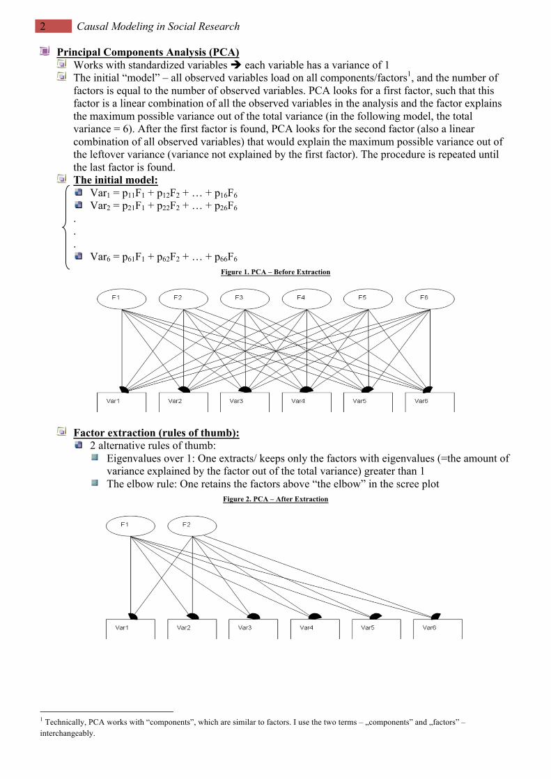
Principal Components Analysis (PCA) Works with standardized variables è each variable has a variance of 1 The initial “model” – all observed variables load on all components/factors1, and the number of

factors is equal to the number of observed variables. PCA looks for a first factor, such that this factor is a linear combination of all the observed variables in the analysis and the factor explains the maximum possible variance out of the total variance (in the following model, the total variance = 6). After the first factor is found, PCA looks for the second factor (also a linear combination of all observed variables) that would explain the maximum possible variance out of the leftover variance (variance not explained by the first factor). The procedure is repeated until the last factor is found.

The initial model: Var1 = p11F1 + p12F2 + … + p16F6 Var2 = p21F1 + p22F2 + … + p26F6

.

.

. Var6 = p61F1 + p62F2 + … + p66F6

Figure 1. PCA – Before Extraction

Factor extraction (rules of thumb): 2 alternative rules of thumb:

Eigenvalues over 1: One extracts/ keeps only the factors with eigenvalues (=the amount of variance explained by the factor out of the total variance) greater than 1

The elbow rule: One retains the factors above “the elbow” in the scree plot Figure 2. PCA – After Extraction

1 Technically, PCA works with “components”, which are similar to factors. I use the two terms – „components” and „factors” – interchangeably.


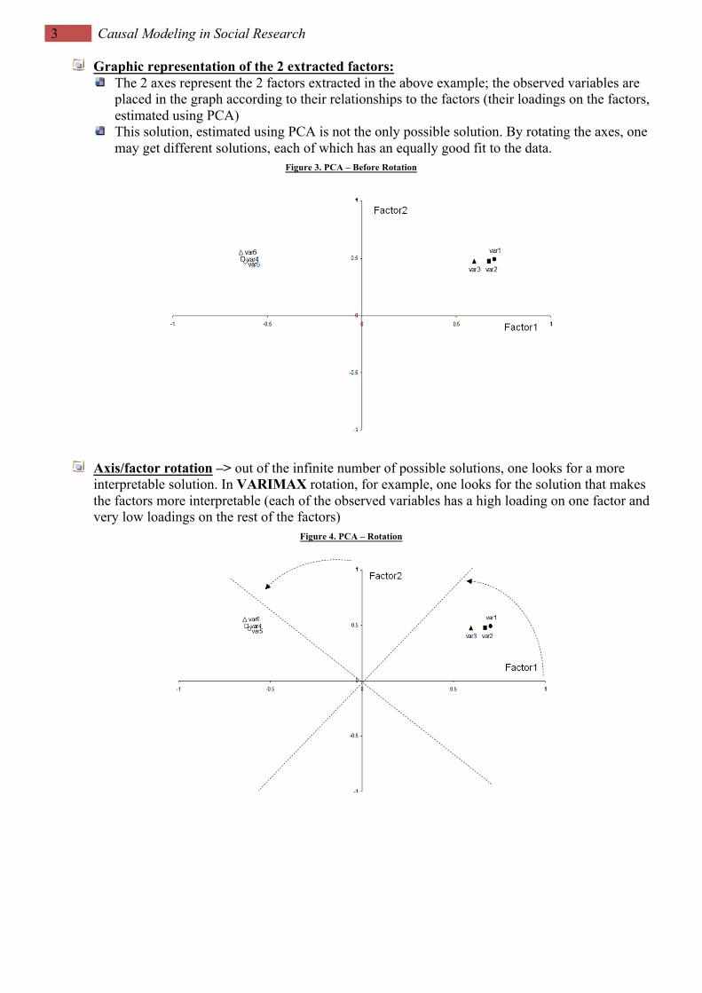
Graphic representation of the 2 extracted factors: The 2 axes represent the 2 factors extracted in the above example; the observed variables are

placed in the graph according to their relationships to the factors (their loadings on the factors, estimated using PCA)

This solution, estimated using PCA is not the only possible solution. By rotating the axes, one may get different solutions, each of which has an equally good fit to the data.

Figure 3. PCA – Before Rotation

Axis/factor rotation –> out of the infinite number of possible solutions, one looks for a more interpretable solution. In VARIMAX rotation, for example, one looks for the solution that makes the factors more interpretable (each of the observed variables has a high loading on one factor and very low loadings on the rest of the factors)

Figure 4. PCA – Rotation


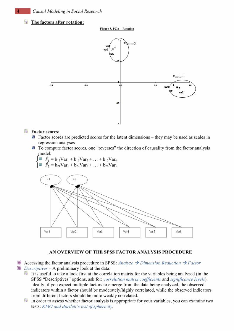
The factors after rotation: Figure 5. PCA – Rotation

Factor scores:

Factor scores are predicted scores for the latent dimensions – they may be used as scales in regression analyses

To compute factor scores, one “reverses” the direction of causality from the factor analysis model:

𝐹" = b11Var1 + b12Var2 + … + b16Var6 𝐹# = b21Var1 + b22Var2 + … + b26Var6

AN OVERVIEW OF THE SPSS FACTOR ANALYSIS PROCEDURE

Accessing the factor analysis procedure in SPSS: Analyze à Dimension Reduction à Factor Descriptives – A preliminary look at the data:

It is useful to take a look first at the correlation matrix for the variables being analyzed (in the SPSS “Descriptives” options, ask for: correlation matrix coefficients and significance levels). Ideally, if you expect multiple factors to emerge from the data being analyzed, the observed indicators within a factor should be moderately/highly correlated, while the observed indicators from different factors should be more weakly correlated.

In order to assess whether factor analysis is appropriate for your variables, you can examine two tests: KMO and Bartlett’s test of sphericity.


KMO is a test that determines whether partial correlations among the observed variables are high enough. Conventionally, KMO values lower than 0.6 suggest that the partial correlations are not high enough and the variables won’t ‘factor’ well.

Bartlett’s test has the following null hypothesis (H0): the correlation matrix for the observed variables is an identity matrix. In other words, the null hypothesis being tested is that all of the observed variables being analyzed are uncorrelated with each other (a situation that is not desirable when doing factor analysis). A statistically significant Bartlett’s test suggests that at least one of the correlations between your observed variables is different from zero (the H0 of the test can be rejected).

Note: In practice, if the purpose of the analysis is to extract factors that will be used in other analyses (e.g. regression analyses) as independent or dependent variables, it is also useful to take a look at the relationships between each of the variables used in the factor analysis and the other variables that will be employed in the final model (Treiman, 2009: 247).

Also, as a preliminary step to running a factor analysis, you should make sure that the measurement level of the variables employed in the analysis is appropriate. Interval-level measurement for the observed variables is required in most types of factor analyses (the SPSS factor analysis procedure is technically designed for this type of variables only). In practice, ordinal level observed variables may be used as well, as long as one can make the assumption that these variables are ‘interval-like’ variables. If you are dealing with other types of indicators (for example dichotomous variables), there is specialized software that can be used to run factor analysis (e.g.: Mplus).

Extraction methods – the method/mathematical model used in order to extract the factors. SPSS provides several options here. The most commonly used (and the default in SPSS): Principal Components Analysis (PCA). It is not a statistical model per se, but a mathematical model for extracting the factors, and it is the simplest and most intuitive model. It extracts uncorrelated (orthogonal factors), although correlated factors can be obtained through a method of oblique rotation (see below), and it disregards the error part/ unique variance/ noise in the variables being included in the analysis.

Cut-off criteria for extracting factors: Eigenvalues over one criterion (SPSS default, found under the ‘Extract’ heading in the

‘Extraction’ window) Fixed number of factors (the user specifies the number of factors to be extracted, found under

the ‘Extract’ heading in the ‘Extraction’ window) The ‘elbow’ rule (applied by inspecting the scree plot, found under the ‘Display’ heading in

the ‘Extraction’ window) Rotation methods – methods used in order to choose one solution from the infinite number of

solutions from an exploratory factor analysis. There are several options here as well: Methods that result in orthogonal (uncorrelated) factors:

Varimax –> makes the factors more interpretable Quartimax –> makes the variables more interpretable Equamax –> a hybrid between the two previous methods

Methods that result in oblique (correlated) factors: Direct Oblimin –> you can control the size of the correlation between factors by manipulation

the ‘delta’ parameter (the default is 0, and results in a solution in which the factors are prevented from being highly correlated; you can increase the value of the delta parameter up to 0.8, resulting in the most oblique solution or you can decrease the value of the delta parameter down to -0.8, resulting in the least oblique solution)

Promax –> a similar procedure as the one above, designed for larger datasets Constructing and saving factor scores (options found in the ‘Scores’ window).

To have SPSS construct a factor score based on your factor analysis results, check the option ‘Save as variables’ in the ‘Scores’ window. If you want to see the factor score coefficients used in the computation of factor scores, check the option ‘Display factor score coefficient matrix’ in the ‘Scores’ window. Available methods for saving factor scores/ computing factor score coefficients:


The regression method (SPSS default): the simplest method, in which the factor loadings resulting from the analysis are adjusted to take into account the initial correlations between the observed variables. The disadvantage of the method: may result in correlated factor scores or factor scores correlated to the other true factors, even if the original factor analysis extracted orthogonal factors. This is the best option when you are not particularly interested in constructing independent factor scores (Field, 2009: 635).

The Bartlett method constructs factor scores that correlate only with their own factor, but factor scores can still correlate with each other.

The Anderson-Rubin method produces uncorrelated factor scores. This is the best option when you need to construct independent factor scores (Field, 2009: 635).

Other options – Finally, you can control some cosmetic but also some substantive aspects of your factor analysis in the ‘Options’ window.

The ‘cosmetic’ options: the rotated solution table is more easily interpretable if the coefficients in that table are sorted by size (check the option ‘Sorted by size’ under the ‘Coefficient display format’ heading); you may also use the option to ‘Suppress small coefficients’ which will delete coefficients smaller than a user-specified value (use this option with caution, especially if you plan to input a different cut-off value, and you are not exactly sure what this option does).

The ‘substantive’ option: how to handle missing data in your analysis. SPSS provides three choices: listwise deletion, pairwise deletion, and replace with mean. Depending on the amount of missing data and patterns of missing data in your variables, each choice may result in dramatically different factor analysis results, and what is worse, all three may result in biased factor analysis results. If the above statement seems very vague, that is because it is intended to be like that. There is a lengthy discussion about missing data and ways to handle it in statistical analyses, and we’ll have that discussion in a couple of lectures from now. SPSS’ default is listwise deletion – that’s fine, as long as you don’t lose a high percentage of cases from your sample by employing it (you can check the effective remaining sample size by asking for ‘Univariate descriptives’ in the Factor Analysis ‘Descriptives’ window).


EXAMPLE 1: CHECKING THE DIMENSIONALITY OF A WELL-BEING SCALE

Data for this analysis: Family Life [Viaţa de Familie] (2008) Data file, Survey designed and executed by Soros Foundation Romania. If you are interested, you can find out more details about this survey here: http://www.fundatia.ro/en/family-life-2008. This is a nationally representative survey conducted in 2008 in Romania (N=1,400). The example will employ an 80% random sample from the nationally representative sample. You can find the data file for the example on the class website (filename: FL2008_random80_wellbeing.sav)

Variables: Among the many variables designed to capture aspects of family life, the survey employed a series of indicators of personal well-being. The wording of the questions is given below.

Note: If you are interested in this dimension and you want to analyze data for other countries, ESS (European Social Survey) employed this scale in Round 2 (2004). You can find out more details about ESS and links to data downloads here: http://www.europeansocialsurvey.org/

Firstly, I am going to read out a list of statements about how you may have been feeling recently. For each statement, using this card, I would like you to say how often you have felt like this over the last two weeks. Please use this card. All of

the time Very often Often Seldom Very seldom Never DK NA

G1. I have felt cheerful and in good spirits 6 5 4 3 2 1 8 9 G2. I have felt calm and relaxed 6 5 4 3 2 1 8 9 G3. I have felt active and vigorous 6 5 4 3 2 1 8 9 G4. I have woken up feeling fresh and rested 6 5 4 3 2 1 8 9 G5. My daily life has been filled with things that interest me

6 5 4 3 2 1 8 9

Theoretically, all indicators should load on a single underlying/latent dimension measuring personal

well-being. In order to check this assumption, one can run an exploratory factor analysis. As preliminary steps to the factor analysis, you should run some frequencies to see if any recodes are

necessary (i.e., in this case, assigning missing values to the DK/NA responses). For this example, we will recode variables G1-G5 into the new variables: CHEERFUL, CALM, ACTIVE, RESTED, INTERESTING

Note: The original database contains a weight variable (weight_vs), designed to adjust the sample composition according to the age by sex distribution in the population. This variable is provided in the FL2008_random80_wellbeing dataset and you might want to weight the data (Data –> Weight Cases –>Weight Cases by –> weight_vs) before proceeding to run the factor analysis in order to insure the generalizability of results to the entire Romanian population.

Factor analysis options for this analysis:


Output interpretation for this analysis: Listwise deletion, employed here as a method of dealing with incomplete data, has resulted in a weighted sample size for the analysis of 1,116 cases (out of the total weighted number of cases: 1,137). The descriptive statistics table below also shows means and standard deviations for the unstandardized version of the variables in the analysis. Since we are using the correlation matrix as an input for the analysis, the actual factor analysis results will pertain to the standardized version of these variables.

Descriptive Statistics Mean Std. Deviation Analysis N

CHEERFUL 3.5915 1.20345 1116 CALM 3.6675 1.16214 1116 ACTIVE 3.8418 1.23429 1116 RESTED 3.6084 1.17998 1116 INTERESTING 3.3939 1.23631 1116

The correlation matrix shows statistically significant, moderate to high correlations among the observed indicators used in the analysis.

Correlation Matrix CHEERFUL CALM ACTIVE RESTED INTERESTING

Correlation CHEERFUL 1.000 .671 .635 .610 .612 CALM .671 1.000 .553 .615 .484 ACTIVE .635 .553 1.000 .640 .561 RESTED .610 .615 .640 1.000 .495 INTERESTING .612 .484 .561 .495 1.000

Sig. (1-tailed) CHEERFUL .000 .000 .000 .000 CALM .000 .000 .000 .000 ACTIVE .000 .000 .000 .000 RESTED .000 .000 .000 .000 INTERESTING .000 .000 .000 .000

The KMO test and Bartlett’s test both suggest that the variables ‘hang together’ well (partial correlations among variables are high enough for a factor analysis, as suggested by the KMO test, and at least one bivariate correlation among variables is non-zero, as suggested by Bartlett’s test).

KMO and Bartlett's Test Kaiser-Meyer-Olkin Measure of Sampling Adequacy. .858 Bartlett's Test of Sphericity Approx. Chi-Square 2745.915

df 10 Sig. .000

The communalities table shows the proportion of variance in each observed variable explained by all of the components/factors. In the initial solution, where the number of factors is equal to the number of observed variables, the 5 factors explain all of the variance in each of the observed variables. After extraction, the smaller number of retained factors explains lower proportions of variance in each of the observed variables.

Communalities Initial Extraction

CHEERFUL 1.000 .750 CALM 1.000 .661 ACTIVE 1.000 .688 RESTED 1.000 .676 INTERESTING 1.000 .581 Extraction Method: Principal Component Analysis.

The eigenvalues show the amount of variance (out of the total variance) explained by each of the factors. Since the observed variables are standardized for this analysis (by default, the input data is the correlation matrix), each of the observed variables in the analysis will have a mean of 0 and a variance of 1. As a result, the total variance (in all observed variables) will equal the number of observed variables in the analysis (5, in this case). The left half of the table below presents information about the eigenvalues for all of the factors in the initial solution, while the right half presents the same information only for the factor(s) that was/were retained after extraction. In this case, we can see that a single factor was retained after extraction (using the default cutoff criterion for extraction: eigenvalues over 1), and that factor explains approximately 67% of the total variance in our 5 observed variables. The remaining factors from the initial solution all have eigenvalues smaller than 1, and are subsequently ‘discarded’ from the final factor analysis solution.


Total Variance Explained

Component Initial Eigenvalues Extraction Sums of Squared Loadings

Total % of Variance Cumulative % Total % of Variance Cumulative % 1 3.356 67.117 67.117 3.356 67.117 67.117 2 .551 11.025 78.142 3 .457 9.145 87.287 4 .347 6.944 94.231 5 .288 5.769 100.000 Extraction Method: Principal Component Analysis. The scree plot (which can be used as an alternative criterion for determining the number of factors to retain after extraction), in this particular case, also suggests that a one-factor solution is appropriate (the ‘elbow’ occurs at the second component, and we may retain the one component that is placed above the elbow). The two criteria for determining the number of factors to be extracted (the ‘eigenvalues over 1’ and the ‘elbow rule’) will not always suggest the same number of factors to extract. In that case, you should decide theoretically and based on the results of a preliminary factor analysis how many factors to extract. You can choose the number of factors to be extracted by using the ‘Fixed number of factors’ option in the ‘Extraction’ window. In terms of our particular interest in running this factor analysis, at this point, we already have an answer to our question: the five observed indicators all load on a single dimension/ measure a single underlying, latent concept. We could label this latent concept as ‘personal well-being’, based on the particular things that the observed indicators measure (auto-evaluations of states of mind associated with a feeling of well-being).

One last thing that we have to do to ensure that all of the observed variables are highly associated with the underlying factor is to check the loadings of these variables on the factor. In the case of a factor analysis that has extracted only one factor, these loadings are found in the ‘Component Matrix’ table. In this example, all loadings are high (over .7).There are various criteria being used to determine what constitutes a high or moderate loading in current research, and rules of thumb are usually different depending on the research topic.

Component Matrixa

Component

1 CHEERFUL .866 ACTIVE .829 RESTED .822 CALM .813 INTERESTING .762 Extraction Method: Principal Component Analysis. a. 1 components extracted. Finally, if you are interested in using the well-being dimension in further analyses, as a summary measure instead of using each and all of the observed indicators, factor analysis provides you with the option of saving predicted factor scores for each individual in the analysis. The factor score coefficients used in the computation of these

10 Causal Modeling in Social Research factor scores are displayed in the ‘Component Score Coefficient Matrix’ table. The resulting factor score variable, saved by SPSS, is a standardized variable, with a mean of 0 and a standard deviation of 1.

Component Score Coefficient Matrix

Component

1 CHEERFUL .258 CALM .242 ACTIVE .247 RESTED .245 INTERESTING .227 Extraction Method: Principal Component Analysis. Component Scores.

Note: If you would like to try some further analyses on your own, using the constructed factor score, the database provided with the example includes a couple of other variables (age, sex, marital status, income, and education).

MORE THAN ONE DIMENSION: THE ‘GETTING AHEAD’ SCALES

Data: Class Structure and Social Stratification in Present Day Romania, 2010 (CNMP, grant: 131/20.11.2008). This is a nationally representative survey conducted in 2010 in Romania (N=4,508). The example will employ a 50% random sample from the nationally representative sample. The database used in this example is available on the class website (filename: STRAT2010_random50_ahead.sav)

Variables: Opinions about prevailing successful strategies for getting ahead in life in Romania. The wording of the questions is given below. Theoretically, the observed indicators should capture 4 dimensions: strategies based on ascription, merit, discrimination, and corruption.

Note: if you are interested in these variables in an international context, they are also employed in the ISSP (International Social Survey Programme), Social Inequality Modules (1992, 1999, 2009). For more details about ISSP and links to data downloads, you can consult the survey webpage: http://www.issp.org/ .

V16. How important are each of the following for a person in present-day Romania to get ahead in life?

Very important Fairly important Neither/nor Fairly

unimportant Not important NA

a. … coming from a wealthy family 5 4 3 2 1 -9 b.… having well-educated parents 5 4 3 2 1 -9 c.… having a good education yourself 5 4 3 2 1 -9 d.… having ambition 5 4 3 2 1 -9 e.… hard work 5 4 3 2 1 -9 f.… knowing the right people 5 4 3 2 1 -9 g.… having political connections 5 4 3 2 1 -9 h.… giving bribes 5 4 3 2 1 -9 i.… belief in God? 5 4 3 2 1 -9 j.… a person’s ethnicity 5 4 3 2 1 -9 k.… a person’s religion 5 4 3 2 1 -9 l.… a person’s gender 5 4 3 2 1 -9

Preliminary steps: variables recodes (missing labels for NA responses) result in the following new variables: wealthfam, educpar, youreduc, ambition, hardwrk, rightppl, polconnect, bribes, gdbelief, pethnic, prelig, pgender. Preliminary analyses suggest that gdbelief does not behave as expected (loads on a different dimension than expected, so we’ll leave it out of the analyses).

Factor analysis options: same as before, with a couple of minor differences. Since we know that theoretically, 4 dimensions are expected to emerge, we can require that 4 factors be extracted. Also, since we are dealing with a multiple factor solution, we can choose a rotation method (we’ll try an orthogonal rotation method – Varimax, and an oblique rotation method – Oblimin).

Differences from a one-factor solution: A new panel added to the ‘Total Variance Explained’ table, containing results for the rotated

solution. In orthogonal rotation variants, factor loadings are presented in the unrotated solution (found in

the ‘Component Matrix’ table) and the rotated solution (‘Rotated Component Matrix’). Since the rotated solution provides more interpretable factors, usually one interprets the loadings in the Rotated Component Matrix Table and disregards the loadings in the Component Matrix Table.


In oblique rotation variants, there are three versions of factor loadings presented: loadings in the unrotated solution (in the ‘Component Matrix’ table), loadings (as regression coefficients) in the rotated solution (in the ‘Pattern Matrix’ table), and loadings (as correlation coefficients) in the rotated solution (in the ‘Structure Matrix’ table). Usually, the factor pattern coefficients are the most informative.

(Substantive) interpretation of loadings (other tests – i.e. KMO and coefficients – i.e. eigenvalues are interpreted in the same way as in the one-factor solution)

Using Varimax rotation, the rotated solution diverges somewhat from an ideal ‘simple structure’ solution (two variables load highly on more than one component: the importance of coming from a wealthy family and the importance of your education). Also, the emerging grouping of variables diverges somewhat from the theoretical expectations (the same two variables mentioned before load on an additional, theoretically unrelated dimension).

Rotated Component Matrixa

Component

1 - Corruption 2 - Discrimination 3 - Merit 4 - Ascription polconnect .862 .105 .019 .014 rightppl .815 .030 .205 .000 bribes .770 .154 -.030 -.006 wealthfam .564 .002 -.092 .555 prelig .003 .907 .020 .040 pethnic .133 .876 -.012 .035 pgender .147 .856 -.068 .010 hardwrk .078 -.009 .873 .088 ambition .079 -.059 .834 .247 educpar .003 .076 .289 .863 youreduc -.100 .019 .571 .671 Extraction Method: Principal Component Analysis. Rotation Method: Varimax with Kaiser Normalization. a. Rotation converged in 5 iterations. The Oblimin solution is very similar to the Varimax solution: the same discrepancies arise.

Pattern Matrixa

Component

1 - Corruption 2 - Merit 3 - Discrimination 4 - Ascription polconnect .863 .016 .039 .011 rightppl .829 .210 -.027 .051 bribes .767 -.030 .096 .024 hardwrk .093 .889 .005 .043 ambition .077 .818 -.049 -.132 prelig -.078 .032 .917 -.015 pethnic .056 -.002 .875 -.013 pgender .074 -.055 .852 .006 educpar -.107 .141 .069 -.864 youreduc -.174 .469 .029 -.621 wealthfam .496 -.201 -.054 -.587 Extraction Method: Principal Component Analysis. Rotation Method: Oblimin with Kaiser Normalization. a. Rotation converged in 9 iterations.

A possible solution is to revise: (a) the interpretation of the ‘importance of coming from a wealthy family’ indicator (it could be

considered as both an indicator of strategies based on ascription but also as a proxy for strategies based on corruption, at least at the public opinion level)

(b) the label for what was supposed to be the ‘ascription-based strategies’ dimension. Given that this dimension is captured by the importance of parental education, of one’s own education, and of coming from a wealthy family, it seems to measure socio-economic resources – based strategies. An alternative explanation could be that some respondents view the educational system rather as a mechanisms of transmitting the advantages in the family of origin (the parents’ education and wealth) rather than as a meritocratic mechanism.

12 Causal Modeling in Social Research DESIRABLE JOB CHARACTERISTICS DIMENSIONS (OPTIONAL QUICK EXAMPLE OF EXPLORATORY FACTOR ANALYSIS WITH CATEGORICAL INDICATORS - MPLUS)

Data: Romanian sample from the EVS (European Values Study), the 2008 wave. You can find out more details about this survey here: http://www.europeanvaluesstudy.eu/ . The survey is a cross-national survey, and the Romanian subsample is a nationally representative sample for the Romanian population.

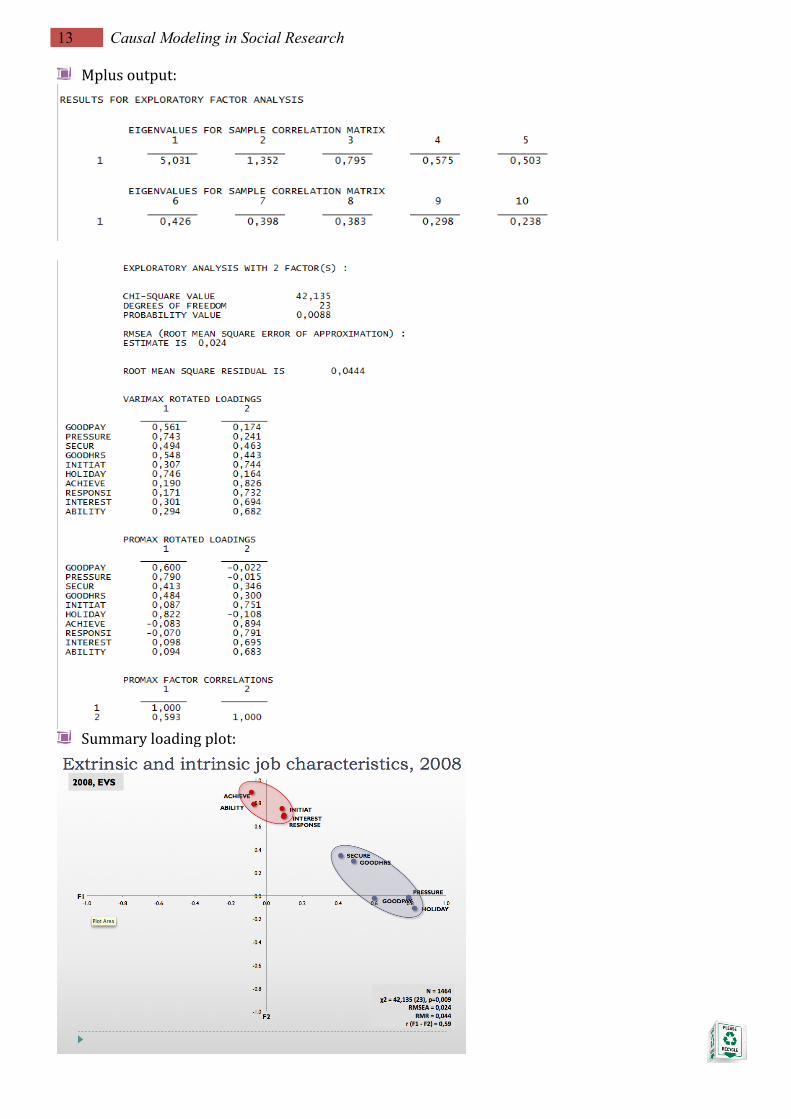
Variables: job characteristics that people consider as being important. Theoretically, the variables (question wording given below) are considered to tap two underlying dimensions: extrinsic and intrinsic motivations in job performance

Here are some aspects of a job that people say are important. Please look at them and tell me which ones you personally think are important in a job? Mentioned Not mentioned Good pay (GOODPAY) 1 0 Good job security (SECURE) 1 0 Not too much pressure (PRESSURE) 1 0 Good hours (GOODHRS) 1 0 Generous holidays (HOLIDAY) 1 0 An opportunity to use initiative (INITIAT) 1 0 A job in which you feel you can achieve something (ACHIEVE) 1 0 A responsible job (RESPONSE) 1 0 A job that is interesting (INTEREST) 1 0 A job that meets one’s abilities (ABILITY) 1 0

Mpluscode:TITLE: EFA 2008 DATA: File is Y:\01_Date\sample2.dat ; VARIABLE: Names are

Myunid SURVYR BIRTHYR AGE goodpay pressure secur Goodhrs initiat holiday achieve response interest ability respect Pleasppl promote useful meetppl learn bal say equal weight;

Usevariables are goodpay - ability; Categorical are goodpay - ability; Missing ARE all (-1234) ; USEOBS SURVYR EQ 2008; WEIGHT IS weight; ANALYSIS: TYPE = efa 1 3; ESTIMATOR = wlsmv ;


Mplusoutput:

Summaryloadingplot:

Exploratory Factor Analysis – Principal Components Analysis · Exploratory Factor Analysis –...

Documents

Transcript of Exploratory Factor Analysis – Principal Components Analysis · Exploratory Factor Analysis –...