1

Revised manuscript Submitted to “Pattern Recognition” on August 11, 2015

Fabric inspection based on the Elo rating method

Colin S. C. Tsang Department of Mathematics

Hong Kong Baptist University, Kowloon Tong, Hong Kong Email: 11019700@life.hkbu.edu.hk

Henry Y. T. Ngan*

Department of Mathematics Hong Kong Baptist University, Kowloon Tong, Hong Kong

Email: ytngan@hkbu.edu.hk Phone: +852-3411-2531

Grantham K. H. Pang

Industrial Automation Research Laboratory Department of Electrical and Electronic Engineering

The University of Hong Kong, Pokfulam Road, Hong Kong Email: gpang@eee.hku.hk

*Corresponding author

2

Abstract

Automated visual inspection of patterned fabrics, rather than of plain and twill fabrics, has

been increasingly focused on by our peers. The aim of this inspection is to detect, identify and

locate any defects on a patterned fabric surface to maintain high quality control in

manufacturing. This paper presents a novel Elo rating (ER) method to achieve defect detection

in the spirit of sportsmanship, i.e., fair matches between partitions on an image. An image can

be divided into partitions of standard size. With a start-up reference point, matches between

various partitions are updated through an Elo point matrix. A partition with a light defect is

regarded as a strong player who will always win, a defect-free partition is an average player

with a tied result, and a partition with a dark defect is a weak player who will always lose.

After finishing all matches, partitions with light defects accumulate high Elo points and

partitions with dark defects accumulate low Elo points. Any partition with defects will be

shown in the resultant thresholded image: a white resultant image corresponds to a light defect

and a grey resultant image corresponds to a dark defect. The ER method was evaluated on

databases of dot-patterned fabrics (110 defect-free and 120 defective images), star-patterned

fabrics (30 defect-free and 26 defective images) and box-patterned fabrics (25 defect-free and

25 defective images). By comparing the resultant and ground-truth images, an overall detection

success rate of 97.07% was achieved, which is comparable to the state-of-the-art methods.

Keywords: Elo rating, Sportsmanship, Match, Partition, Fabric inspection, Defect detection,

Texture analysis, Patterned texture

3

1. INTRODUCTION

Fabric is fundamental to many consumable products in daily life such as clothing, fashions,

bags, bed coverings, nano-scale medical fabrics, and even air-conditioning ducts. Fabric

inspection is a key component of quality control in textile manufacturing. Currently, most

fabric inspection is conducted visually by human workers working at high cost, but it is not

reliable due to human errors and eye fatigue. Automated visual inspection (AVI) of fabric

applies computer vision techniques that offer not only an efficient, low-cost and accurate

approach to replace the labour force but also expansion of inspection capabilities to cover a

broader range of different fabric patterns, from the simplest to the most complicated. The aim

of AVI is to detect and outline the shapes and locations of any defects on a fabric surface during

or after weaving. There is much research on fabric inspection [1] of both simple and

complicated patterned fabrics. This study focuses on fabric with complicated patterns (Fig. 1).

A patterned fabric is composed of a basic fundamental unit, called the motif [2], which can be

generated into the whole pattern by certain rules of symmetry. Based on these predefined rules,

a patterned fabric can be classified into one of seventeen wallpaper groups [2].

Currently, AVI of fabric can be broadly classified into two main categories: motif- and

non-motif-based. A number of methods have been developed for non-motif-based inspection.

Most methods have been designed for the simplest patterns of the p1 group, plain and twill

fabrics [1]. The five representative inspection approaches are statistical (e.g., regularity

4

measure [3], fractal feature [4], morphological filter [5,6]), spectral (e.g., Fourier transforms

[7–9], Gabor [10], wavelet [11–13]), model-based (e.g., Gaussian Markov random field [14],

sparse dictionary reconstruction [15]), learning (e.g., neural network [16], support vector

machine [4]) and structural (e.g., maximum frequency distance [17]). In contrast, only a few

methods target other wallpaper groups, such as wavelet-pre-processed golden image

subtraction (WGIS) [18], direct thresholding (DT) [18], co-occurrence matrix (CM) [19],

Bollinger bands (BB) [20], regular bands (RB) [21] and image decomposition (ID) [22]. The

method developed herein aims to inspect the patterned fabrics of the non-p1 fabric groups.

In this paper, a novel inspection method called the Elo rating (ER) method is proposed

in which fabric inspection is treated as sporting matches between competing partitions

(players). In other words, fabric inspection can be realised as sportsmanship during fairly

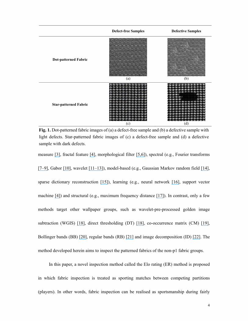
Defect-free Samples Defective Samples

Dot-patterned Fabric

(a)

(b)

Star-patterned Fabric

(c)

(d)

Fig. 1. Dot-patterned fabric images of (a) a defect-free sample and (b) a defective sample with light defects. Star-patterned fabric images of (c) a defect-free sample and (d) a defective sample with dark defects.

5

played matches between competing partitions. The idea of the ER method originates from a

logistic distribution-based statistical system called the Elo rating system, developed by Elo

[23]. This system is used to measure a player’s capability in many international chess matches,

video matches [24] and even in many other international team sports including football,

basketball, major league baseball, etc.

Fabric inspection is treated in the spirit of sportsmanship by the ER method, which

provides a new perspective for the detection of fabric defects. The idea is that each ×

extracted image partition from an × testing image acts like a player. Some partitions are

selected as players and each player is assigned a starting Elo point (W.L.O.G. = 1000 as the

starting number of base points). A player who wins a match gains some Elo points w.r.t. a

formula suggested by Elo [23] based on a logistic distribution; otherwise the player loses some

Elo points. In the long run, the Elo points accumulated are a fair indication of the player’s

performance even though some players do not encounter each other in the matches. In

patterned fabric defect detection, image partitions of a patterned fabric image are considered

the players and a match is regarded as the matrix operation between these partitions.

According to a score matrix of the ER method, a partition with light defective regions

(Fig. 1(b)) will act like a strong player who tends to achieve a high score in the match and

probably wins many matches. A partition with dark defective regions (Fig. 1(d)) will act like a

weak player who tends to have a low score in the match and probably loses many matches. A

partition that is defect-free will act like an ordinary player who tends to have an average score

6

and ties many matches. Hence, a strong player with light defects should be able to gain Elo

points by winning many matches, whereas a weak player with dark defects should lose Elo

points by losing many matches. Therefore, an area of an image can be indicated as defective

by tracking, partitions with relatively high or low Elo points. Match making in the ER method

is designed as follows. For each partition (player), a certain number of other partitions (players)

are randomly selected to have matches against it. The Elo points of a corresponding player will

be updated after each match. In this paper, dot-, box-, and star-patterned fabrics comprising a

total of 336 images (165 defect-free and 171 defective) are used.

This paper makes the following contributions to the literature.

1. A new application of the ER method is constructed by transforming its theoretical and

physical properties for the purpose of patterned fabric inspection. Four key parameters in the

ER method, including partition size, number of randomly located partitions, − ,

and constant , are carefully justified in the performance evaluation.

2. The ER method provides a binary classification of the nature of the defect in the final

resultant image: white as a light defect, grey as a dark defect and black as defect-free.

3. From fabric databases with ground-truth images, the ER method achieves 96.89%

accuracy for dot-patterned fabrics using 110 defect-free and 120 defective images, 98.82%

accuracy for star-patterned fabrics using 30 defect-free and 26 defective images and 99.07%

for box-patterned fabrics using 25 defect-free and 25 defective images. These results

outperform those of the WGIS method and are comparable to those of the previously developed

7

BB, RB and ID methods in [22].

The remainder of this paper is organized as follows. In section 2, we survey the literature

on the detection of patterned fabric defects. Section 3 outlines the ER method and its

procedures. In section 4, we evaluate the performance of the ER method and compare it with

the WGIS, BB, RB and ID methods. Lastly, section 5 concludes the paper.

II. LITERATURE REVIEW ON DEFECT DETECTION IN PLAIN AND TWILL FABRICS

The AVI techniques for fabrics in motif-based classification [25] can be divided into two

main categories. Only a few methods have been developed for the patterned fabrics of the non-

p1 wallpaper group. Research into the inspection of these patterned fabrics has been increasing

in the last decade. The developed methods can be classified into four approaches: statistical,

spectral, model-based and learning approaches.

The statistical approach includes gray relational analysis with CM features [19] on

Jacquard fabric images to study correlations between the analysed factors of chosen features

from a randomised factor sequence. This method reached 94% detection accuracy for 50

defective samples in [19]. The spectral approach includes many methods, such as WGIS [18],

DT [18], wavelet-decomposition [26], template matching for discrepancy measure (TMPM)

[27], BB [20], RB [21] and a Gabor filter [28]. The WGIS method [18] used a golden image

to perform moving subtraction of each pixel along each row of every wavelet-pre-processed

tested image. It generated 96.7% accuracy on 30 defect-free and 30 defective patterned images

(pmm group). The DT method [18] applied a thresholding technique for defect detection on

8

level 4 of Haar wavelet horizontal and vertical detailed sub-images in the same database for

the WGIS method and generated 88.3% accuracy. Li and Di [26] developed a wavelet-

decomposition method [26] to improve the DT method by extracting Haar level 2 high-

frequency coefficients as the vertical detailed sub-image for thresholding and applied a

morphological filter to remove noise on a detected image. However, only one inspection on a

knitted fabric sample was published. Stubl et al. [27] used a golden image-like approach to

exploit a discrepancy measure as a fitness function to detect defects on patterned textures. They

evaluated the TMPM method on the TILDA database (no details on the wallpaper group) and

achieved 96.1% correct detection. The BB and RB methods, designed by different

combinations of moving average and standard deviation, used the regularity property of a

patterned texture to carry out defect detection on dot-, box- and star-patterned fabrics (p2, pmm

and p4m groups, respectively). The BB and RB methods obtained accuracy rates of 98.59%

(167 defect-free and 171 defective images) and 99.4% (80 defect-free and 86 defective images),

respectively. Raheja et al. [28] proposed a Gabor filter method and a gray-level CM method

that were then evaluated on 60 defect-free and defective samples (no details on the wallpaper

group) from various fabrics with 98.33% and 95% correct detection, respectively.

The model-based approach includes a recent ID method [22] that decomposed a fabric

image into structures of cartoon (defective objects) and texture (repeated patterns). The ID

method resulted in detection accuracies ranging from 94.9%-99.6% for the dot-, box- and star-

patterned fabrics. The ID method is carried out in a semi-supervised approach which is

9

different to the WGIS, BB and RB methods which are performed in a supervised approach.

Lastly, in the learning approach, Li et al. [29] applied a spectral estimation technique to extract

pattern features and fed them into a rough set classifier. They obtained 95.3% detection

accuracy for a patterned fabric database (p4m group), in which 100 samples were used for

training and 120 samples were used for testing.

In short, no previous method has viewed fabric inspection as a series of matches between

any two partitions of the image. A novel use of the ER method for fabric defect detection is

thus presented.

III. THE ER METHOD

3.1 Definitions for the ER method

Definition 1 (Score of a competition). For an image of size × , say , which has a match

with another image of size × , say , the score s for is defined by

s = ∑ ∑ ( , − , ). (1)

Definition 2 (Expected value of a win). Suppose the Elo points of images and with size

× before a match are and respectively. The expected value of winning the match,

according to logistic distribution, is defined as

= ( )/ . (2)

Without loss of generality, the starting Elo points of and are both set at 1000. In

(2), and are the respective probabilities of and winning the game. Hence,

note the mathematical property below:

10

+ = ( )/ + ( )/ = // / + // / = 1. (3)

As suggested by Elo [23], w = 400, which is called the − of the ER system,

is set arbitrarily. For example, the Elo points of any image are stabilized at the loser being

600 = − 400 or at the winner being 1400 = + 400. If the number is large, the rating scale will be stretched out.

Definition 3 (Elo points update). After a match, the new Elo points of an image are defined

by

= + ( − ). (4)

where is the original Elo points, is the updated Elo points, is a constant (K = 16 is

used here) and − should be in between -1 and 1:

= 1 ℎ ℎ 0.5 ℎ ℎ0 ℎ ℎ . (5)

The constant in (4), regarded as the maximum Elo points an image can gain or lose in one

match, can be set arbitrarily, but its scale would be excessive at a large value. If = 16 and

= 400, an image of “high skill level to win matches” will gain around 10 Elo points per

win, and vice versa. Similarly, an image’s Elo points will be stabilized at 1400 = + 400 if the image continues to win matches, and vice versa.

The image in Definitions 1-3 above means the partition as described below.

3.2 Procedures of the ER method

The ER method involves three main phases: (A) acquisition of a score matrix, (B) the

11

training stage and (C) the testing stage.

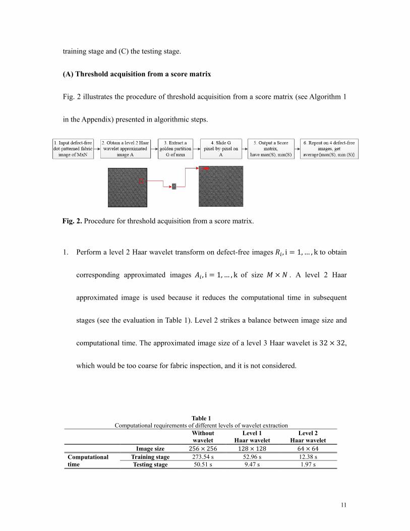
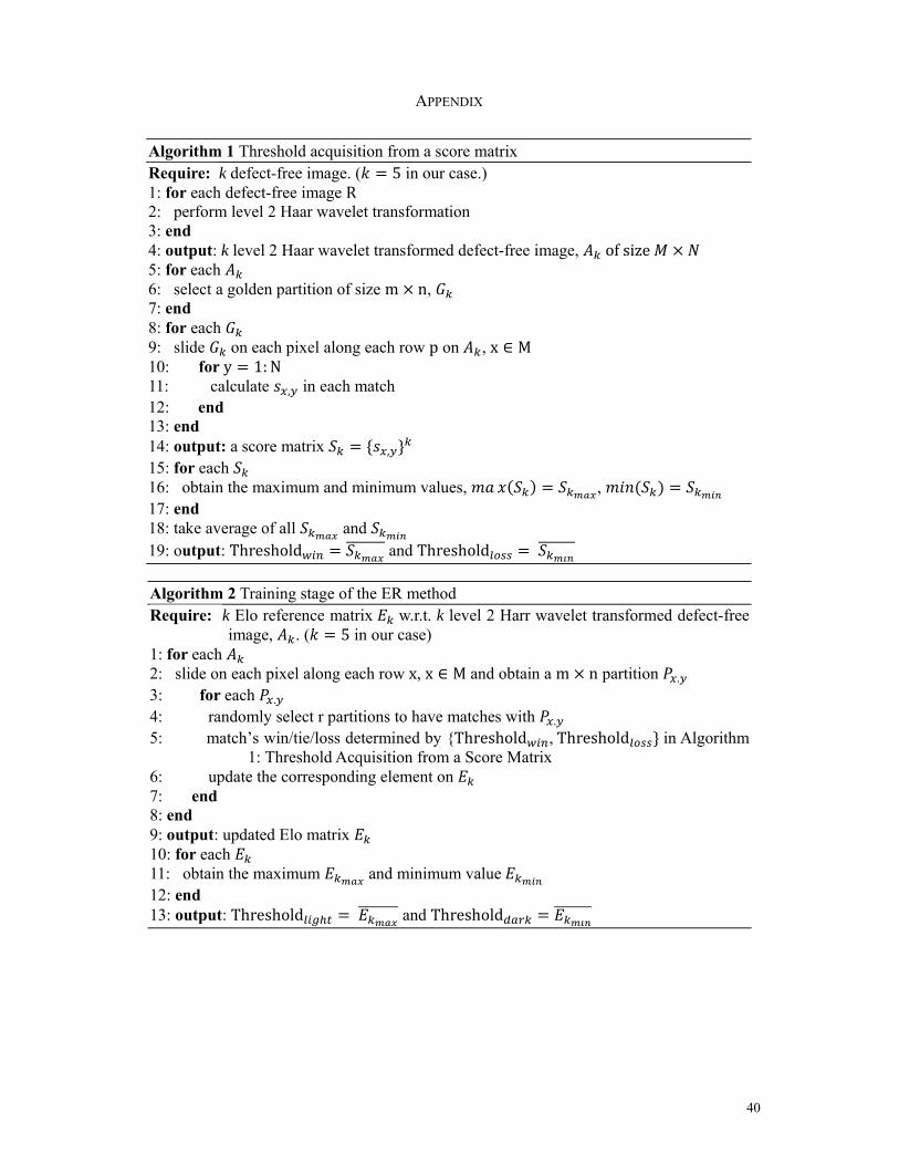
(A) Threshold acquisition from a score matrix

Fig. 2 illustrates the procedure of threshold acquisition from a score matrix (see Algorithm 1

in the Appendix) presented in algorithmic steps.

1. Perform a level 2 Haar wavelet transform on defect-free images , i = 1, … , k to obtain

corresponding approximated images , i = 1, … , k of size × . A level 2 Haar

approximated image is used because it reduces the computational time in subsequent

stages (see the evaluation in Table 1). Level 2 strikes a balance between image size and

computational time. The approximated image size of a level 3 Haar wavelet is 32 × 32,

which would be too coarse for fabric inspection, and it is not considered.

Fig. 2. Procedure for threshold acquisition from a score matrix.

Table 1 Computational requirements of different levels of wavelet extraction

Without wavelet

Level 1 Haar wavelet

Level 2 Haar wavelet

Image size 256 × 256 128 × 128 64 × 64 Computational time

Training stage 273.54 s 52.96 s 12.38 s Testing stage 50.51 s 9.47 s 1.97 s

12

2. For each × level 2 Haar wavelet transformed approximated image, extract a golden

partition of size × , where × is roughly half the dimensions of the length and

width of a motif (each patterned texture is generated by a motif [2]).

3. Slide on each pixel along each row p on . For each move of the sliding process,

record the corresponding score , in each match, where x ∈ M, y ∈ N.

4. Output a score matrix = { , } of size ( − + 1) × ( − + 1) and extract

( ) and ( ).

5. Repeat steps 1-4 for four defect-free sample images (as k = 5 in total). Thus we can define

ℎ ℎ = ( ) = and ℎ ℎ = ( ) = ,

where the bar sign means to obtain either the average value of all ( ) or that of all

( ).

6. Determine a win/tie/loss for any given match, with the interval between Threshold

and Threshold used as below.

If > ℎ ℎ , the match is defined as a win.

If ℎ ℎ < < ℎ ℎ , the match is defined as a tie.

If < ℎ ℎ , the match is defined as a loss.

(B) Training stage

1. Perform level 2 Haar wavelet transform on a defect-free image to obtain approximated

images of size × (see Algorithm 2 in the Appendix for details).

13

2. Divide the approximated images into many partitions. Extract ( − + 1) × ( − +1) partitions for each of size × . For example, the approximated image of a dot-

patterned fabric image is of size 64 × 64 and its motif is roughly of size 7×4. Therefore,

(64 − 7 + 1) × (64 − 4 + 1) = 58 × 61 = 3538 partitions of size 7 × 4 are extracted

for each sample. Name these partition . , . , … , . according to their location.

3. Assign each partition a starting Elo points value (1000 is assigned here). Hence, a

reference matrix of Elo points = (1000) × is obtained for future update.

4. Perform a random locating process to have pairs of (x, y)-coordinates. For randomly

located partitions, say ( , ) , ,…, (i.e., for each x-coordinate [ , , … , ] and y-

coordinate [ , , … , ] , we randomly pick locations. Thus we have

[ , , … , ] and [ , , … , ]). 5. Starting from . , . will have R matches with ( , ), with the result of each match

(win/tie/loss) decided by step 6 of (A). After each match, the corresponding location on

the Elo point matrix will be updated by Definition 3 (Elo point update). Then obtain a

new set of random located partitions ( , ) by repeating step 4.

6. Keep sliding on each pixel on each row , so we can repeat step 5 from , ,

7. After step 6 has finished, an updated Elo point matrix E is obtained:

, , … …⋮ ⋮ ⋱ ⋮… … … , . (5)

Extract ( ) and ( ).

14

8. Repeat steps 1-7 for five defect-free sample images. Thus, it has

ℎ ℎ = ( ) and ℎ ℎ = ( ).

9. Update the Elo point matrix of a test image. If , > ℎ ℎ , the partition ,

is defined as light defective (shown as white in the final image). If ℎ ℎ <, < ℎ ℎ , the partition , is defined as defect-free. If , <

ℎ ℎ , the partition , is defined as dark defective (shown as grey in the final

image).

(C) Testing Stage

1. Carry out steps 1-6 of the training stage of Elo points to obtain an updated Elo point matrix

E of a defective image.

2. Perform defect detection according to step 9 of the training stage.

3. Output a three-colour (black-grey-white) resultant image U:

, , … …⋮ ⋮ ⋱ ⋮… … … , . (6)

If , is light defective, , = 1 (shown as white in the final image).

If , is dark defective, , = 0.5 (shown as grey in the final image).

If , is defect-free, , = 0 (shown as black in the final image).

3.3 Application of a median filter on U to remove noise

A fabric sample with a light defect will be shown as a white resultant image and a fabric

sample with dark defect will be shown as a grey resultant image for visualisation purposes. Fig.

15

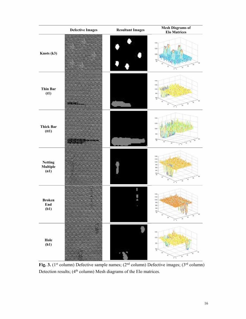
3 shows examples of final resultant images from the ER method with their corresponding mesh

diagrams. A defective sample of Knots (k3) in the second column is considered a light defect

and shows a white resultant image, whereas the defective samples of Thin Bar (t1), Thick Bar

(tt1), Netting Multiple (n1), Broken End (b1) and Hole (h1) are regarded as dark defects and

are shown as grey resultant images.

16

Defective Images Resultant Images Mesh Disgrams of Elo Matrices

Knots (k3)

Thin Bar (t1)

Thick Bar (tt1)

Netting Multiple

(n1)

Broken End (b1)

Hole (h1)

Fig. 3. (1st column) Defective sample names; (2nd column) Defective images; (3rd column) Detection results; (4th column) Mesh diagrams of the Elo matrices.

17

IV. PERFORMANCE EVALUATION

In total, 336 images of size 256 × 256 in 24-bit depth from the dot-, box- and star-

patterned fabric databases are used for evaluation. The dot-patterned fabric database contains

110 defect-free and 120 defective images, the star-patterned database contains 30 defect-free

and 26 defective images, and the box-patterned fabric database contains 25 defect-free and 25

defective images. All defective images have corresponding binary ground-truth images that

illustrate the defective regions as white (value 1) and the defect-free regions as black (value 0).

Performance evaluation is carried out in two progressive steps. In the first step, the number of

white pixels in the final resultant image is obtained. In the second step, a number of

measurement metrics are obtained, namely true positive (TP), false positive (FP), true negative

(TN), false negative (FN), detection success rate (DSR), true positive rate (TPR), false

positive rate (FPR), positive predictive value (PPV) and negative predictive value (NPV). The

details of these metrics are provided in [22].

In the first step, the number of white/grey pixels extracted by the thresholding in the ER

method is obtained. However, this cannot fully reveal the detection performance because the

white/grey pixels can actually be false alarms. Therefore, the second step provides a detailed

analysis. The TPR and FPR are useful for an analysis of the TPR-FPR graph. The PPV can

also be treated as a measure of precision on the fraction of the TP cases among the number of

positive calls in inspection. These metrics assist us in verifying how the ER method performs

with various patterns. We use a desktop computer with an AMD Athlon™ X4 740 Quad Core

18

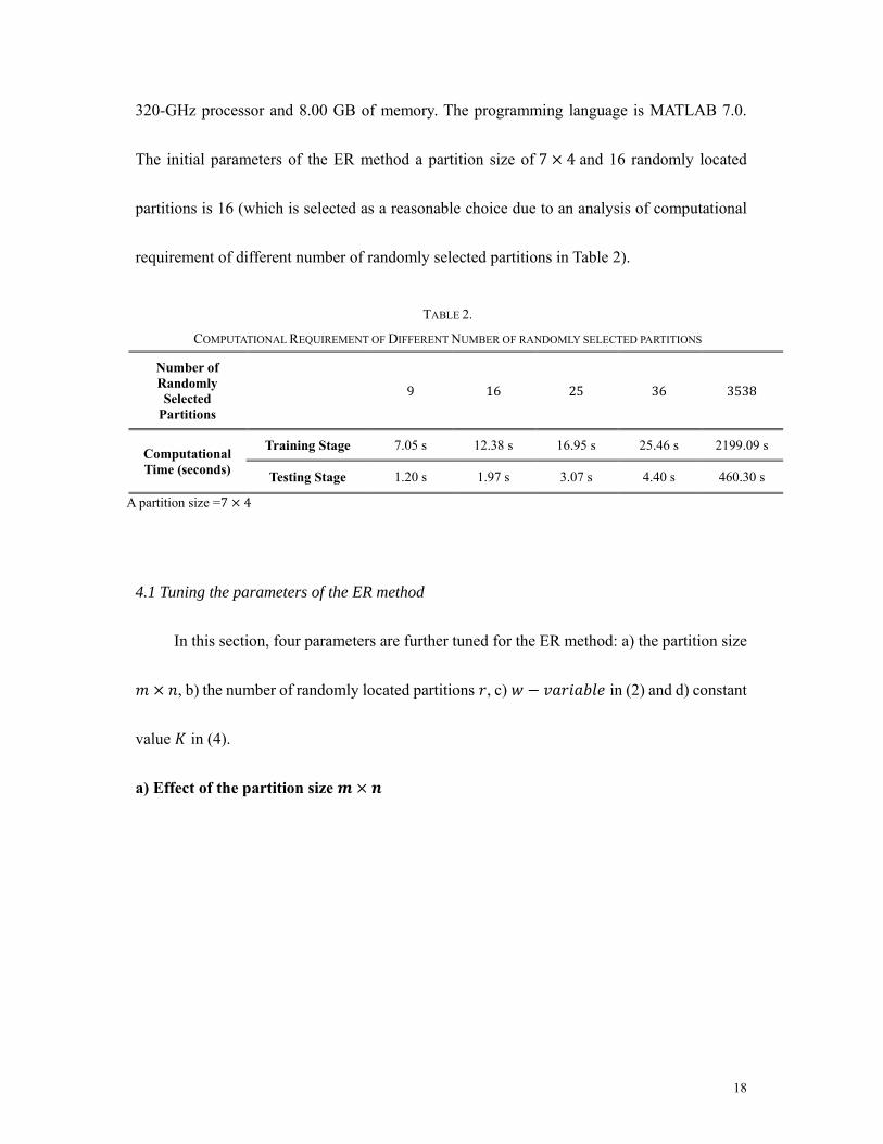
320-GHz processor and 8.00 GB of memory. The programming language is MATLAB 7.0.

The initial parameters of the ER method a partition size of 7 × 4 and 16 randomly located

partitions is 16 (which is selected as a reasonable choice due to an analysis of computational

requirement of different number of randomly selected partitions in Table 2).

4.1 Tuning the parameters of the ER method

In this section, four parameters are further tuned for the ER method: a) the partition size

× , b) the number of randomly located partitions , c) − in (2) and d) constant

value in (4).

a) Effect of the partition size ×

TABLE 2.

COMPUTATIONAL REQUIREMENT OF DIFFERENT NUMBER OF RANDOMLY SELECTED PARTITIONS

Number of Randomly Selected

Partitions 9 16 25 36 3538

Computational Time (seconds)

Training Stage 7.05 s 12.38 s 16.95 s 25.46 s 2199.09 s

Testing Stage 1.20 s 1.97 s 3.07 s 4.40 s 460.30 s

A partition size =7 × 4

19

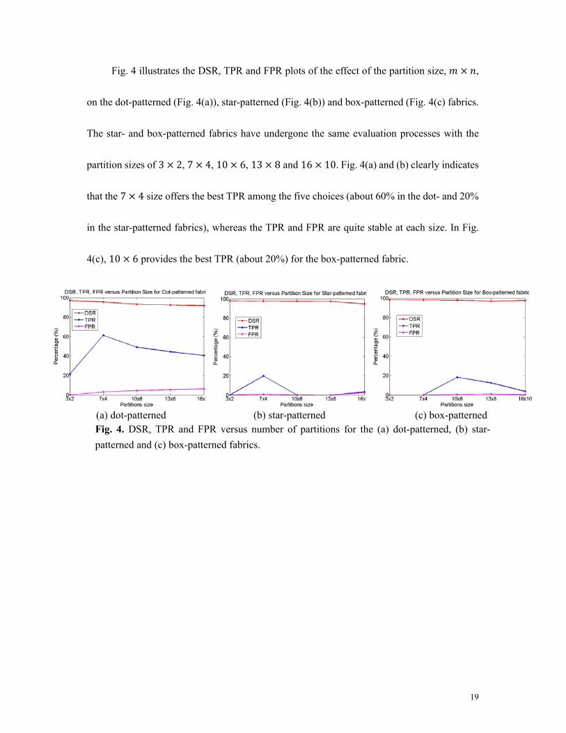
Fig. 4 illustrates the DSR, TPR and FPR plots of the effect of the partition size, × ,

on the dot-patterned (Fig. 4(a)), star-patterned (Fig. 4(b)) and box-patterned (Fig. 4(c) fabrics.

The star- and box-patterned fabrics have undergone the same evaluation processes with the

partition sizes of 3 × 2, 7 × 4, 10 × 6, 13 × 8 and 16 × 10. Fig. 4(a) and (b) clearly indicates

that the 7 × 4 size offers the best TPR among the five choices (about 60% in the dot- and 20%

in the star-patterned fabrics), whereas the TPR and FPR are quite stable at each size. In Fig.

4(c), 10 × 6 provides the best TPR (about 20%) for the box-patterned fabric.

(a) dot-patterned (b) star-patterned (c) box-patterned

Fig. 4. DSR, TPR and FPR versus number of partitions for the (a) dot-patterned, (b) star-patterned and (c) box-patterned fabrics.

20

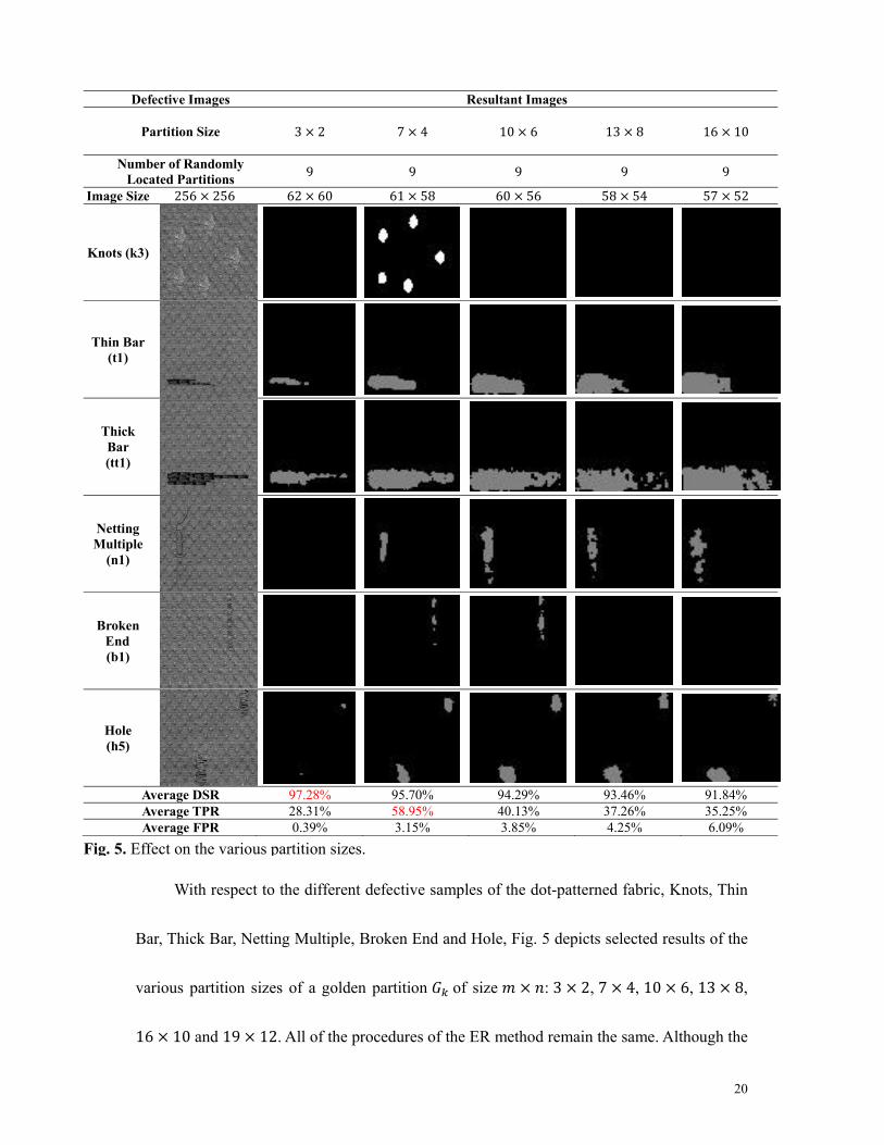
With respect to the different defective samples of the dot-patterned fabric, Knots, Thin

Bar, Thick Bar, Netting Multiple, Broken End and Hole, Fig. 5 depicts selected results of the

various partition sizes of a golden partition of size × : 3 × 2, 7 × 4, 10 × 6, 13 × 8,

16 × 10 and 19 × 12. All of the procedures of the ER method remain the same. Although the

Defective Images Resultant Images

Partition Size 3 × 2 7 × 4 10 × 6 13 × 8 16 × 10

Number of Randomly Located Partitions 9 9 9 9 9

Image Size 256 × 256 62 × 60 61 × 58 60 × 56 58 × 54 57 × 52

Knots (k3)

Thin Bar (t1)

Thick Bar (tt1)

Netting Multiple

(n1)

Broken End (b1)

Hole (h5)

Average DSR 97.28% 95.70% 94.29% 93.46% 91.84% Average TPR 28.31% 58.95% 40.13% 37.26% 35.25% Average FPR 0.39% 3.15% 3.85% 4.25% 6.09%

Fig. 5. Effect on the various partition sizes.

21

size 3 × 2 generates the highest average DSR of 97.28%, it actually misses many true

defective regions. In contrast, the metric TPR reveals the performance more accurately: the

size 7 × 4 provides an average TPR of 58.95%, which is the highest among the three options.

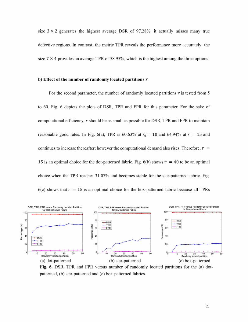
b) Effect of the number of randomly located partitions

For the second parameter, the number of randomly located partitions is tested from 5

to 60. Fig. 6 depicts the plots of DSR, TPR and FPR for this parameter. For the sake of

computational efficiency, should be as small as possible for DSR, TPR and FPR to maintain

reasonable good rates. In Fig. 6(a), TPR is 60.63% at = 10 and 64.94% at = 15 and

continues to increase thereafter; however the computational demand also rises. Therefore, =15 is an optimal choice for the dot-patterned fabric. Fig. 6(b) shows = 40 to be an optimal

choice when the TPR reaches 31.07% and becomes stable for the star-patterned fabric. Fig.

6(c) shows that = 15 is an optimal choice for the box-patterned fabric because all TPRs

(a) dot-patterned

(b) star-patterned

(c) box-patterned

Fig. 6. DSR, TPR and FPR versus number of randomly located partitions for the (a) dot-patterned, (b) star-patterned and (c) box-patterned fabrics.

22

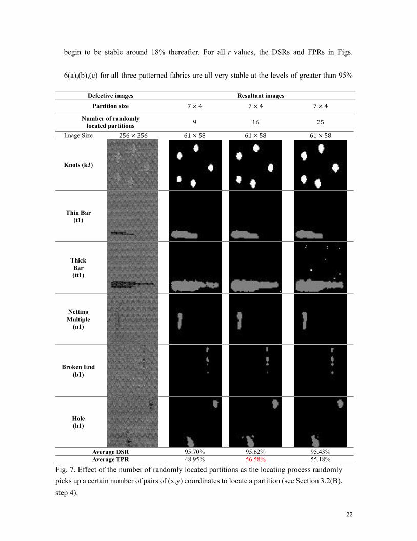
begin to be stable around 18% thereafter. For all values, the DSRs and FPRs in Figs.

6(a),(b),(c) for all three patterned fabrics are all very stable at the levels of greater than 95%

Defective images Resultant images Partition size 7 × 4 7 × 4 7 × 4

Number of randomly located partitions 9 16 25

Image Size 256 × 256 61 × 58 61 × 58 61 × 58

Knots (k3)

Thin Bar (t1)

Thick Bar (tt1)

Netting Multiple

(n1)

Broken End (b1)

Hole (h1)

Average DSR 95.70% 95.62% 95.43% Average TPR 48.95% 56.58% 55.18%

Fig. 7. Effect of the number of randomly located partitions as the locating process randomly picks up a certain number of pairs of (x,y) coordinates to locate a partition (see Section 3.2(B), step 4).

23

and less than 5%, respectively.

Fig. 7 shows the results when the choices of are 9, 16 and 25 for dot-patterned fabric.

In Fig. 6(a), the average DSR is shown to very stable, around 95%, across the variation in the

number of randomly located partitions. The TPR increases from 49.30% to 69.50% when

rises from 5 to 60. The FPR remains relatively stable at 4% at around 25 along the range of 5

and 60. The increase in does cause an increasing noise effect in the detection. For example,

when ≥ 20, noise appears in the final result of some defect types such as Thick Bar in Fig.

7. In the third row of Fig. 7, noise appears only in Thick Bar (tt1) because its defective area is

too large (around 1/4 of the image). Therefore, when is high, a defect-free partition will have

a relatively high probability of matching a defective partition. Thus, defect-free partitions can

gain a number of Elo points by matching with those defective partitions. As a result, many

defect-free partitions are misclassified as light defects. It can be seen that = 16 is a good

trade-off for the dot-patterned fabric, for which the is very close to 15.

c) Effect of the −

The − determines the number of Elo points to be gained or lost per match.

If the difference in original Elo points between partitions and (i.e., − before the

match) is larger than − , then the ER method will predict this match as a “must

win” for partition . Hence, partition will gain a low number of Elo points if it truly wins

this match; otherwise, it will lose a large number of Elo points for the loss of this match. In

24

other words, the − is capable of strengthening the small differences between the

partitions in the image. The advantage of using a small − is to intensify the small

differences between any two partitions. Its shortcoming is that it may overemphasise the

differences, sometimes leading the ER method to mistakenly treat a pattern as a defect. Thus,

in fabric inspection, a small − should be used if the contrast in a pattern is large.

Conversely, a large − should be used for a low-contrast pattern.

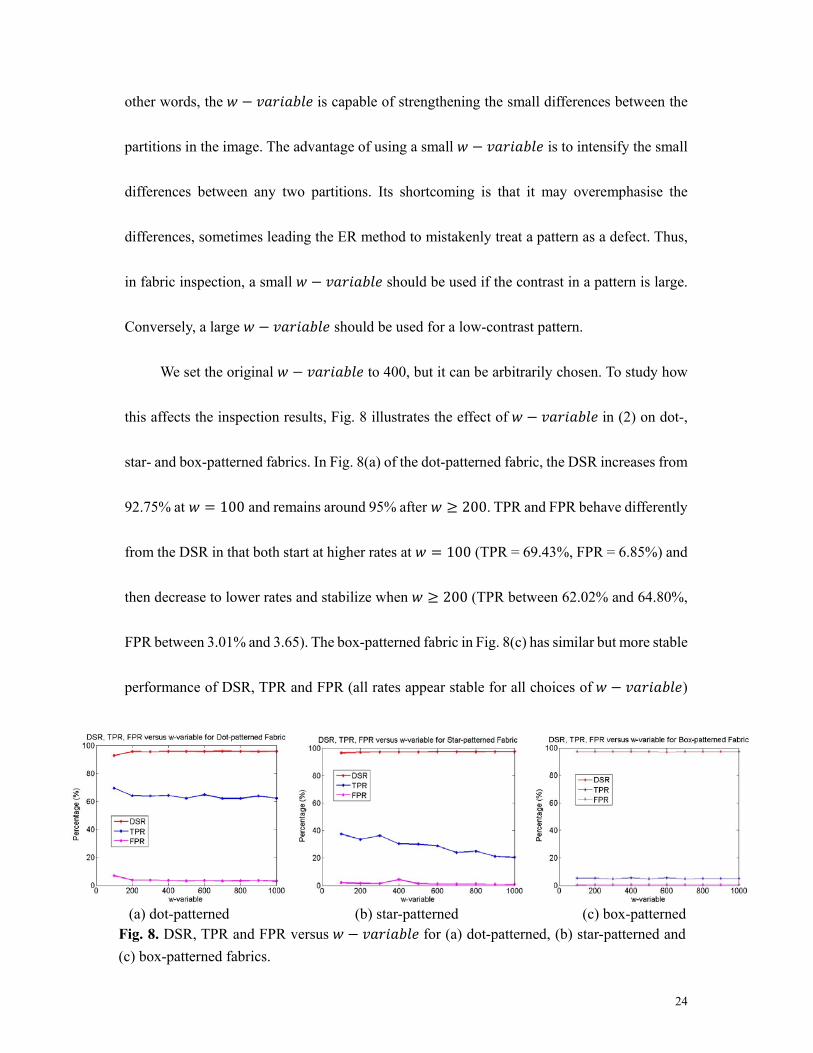
We set the original − to 400, but it can be arbitrarily chosen. To study how

this affects the inspection results, Fig. 8 illustrates the effect of − in (2) on dot-,

star- and box-patterned fabrics. In Fig. 8(a) of the dot-patterned fabric, the DSR increases from

92.75% at = 100 and remains around 95% after ≥ 200. TPR and FPR behave differently

from the DSR in that both start at higher rates at = 100 (TPR = 69.43%, FPR = 6.85%) and

then decrease to lower rates and stabilize when ≥ 200 (TPR between 62.02% and 64.80%,

FPR between 3.01% and 3.65). The box-patterned fabric in Fig. 8(c) has similar but more stable

performance of DSR, TPR and FPR (all rates appear stable for all choices of − )

(a) dot-patterned (b) star-patterned (c) box-patterned

Fig. 8. DSR, TPR and FPR versus − for (a) dot-patterned, (b) star-patterned and (c) box-patterned fabrics.

25

compared with the dot-patterned fabric. The stable performance is actually due to the low

contrast of the dot- and box-patterned fabrics. If − is set to equal 100, it will

overemphasise the differences between any two partitions and the ER method will mistakenly

treat a dot or box pattern as a defect. This problem can be immediately resolved by using a

large − . Therefore, all three measurement matrices stabilise with a large − at 400 in the dot- and box-patterned fabrics.

In Fig. 8(b) of the star-patterned fabric, the contrast is very large (the star pattern is

completely white and the background region is completely dark) so that the ER method easily

misclassifies the star pattern as a defect. The best TPR is 37.49% at = 100, whereas the

later values of TPR decrease at > 100 . Therefore, a small − (i.e., 100) can

provide a more accurate result in terms of TPR.

d) Effect of the constant

The value of is the maximum or minimum number of Elo points of a player at a

different skill level that can be gained or lost in a single match. It also relates to the speed at

which a partition gains or loses a certain number of Elo points. In Fig. 9, the effect of K behaves

similarly to the effect of the − . acts like a multiplying factor to the − in the ER method. A partition can gain or lose a large number of Elo points if the

difference between two partitions is greater than − . If a large is also used, a

26

partition will quickly gain or lose enough Elo points that the difference between this partition

and other partitions will exceed − .

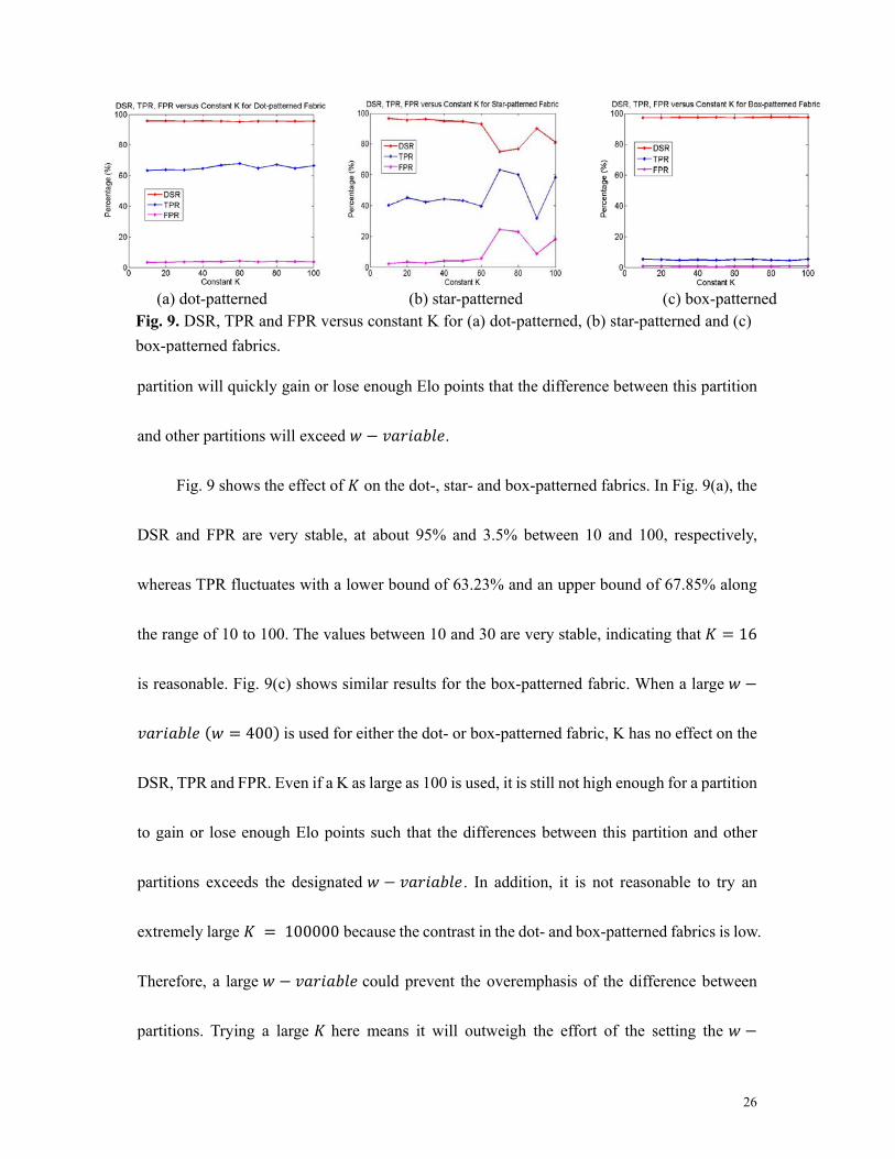
Fig. 9 shows the effect of on the dot-, star- and box-patterned fabrics. In Fig. 9(a), the

DSR and FPR are very stable, at about 95% and 3.5% between 10 and 100, respectively,

whereas TPR fluctuates with a lower bound of 63.23% and an upper bound of 67.85% along

the range of 10 to 100. The values between 10 and 30 are very stable, indicating that = 16

is reasonable. Fig. 9(c) shows similar results for the box-patterned fabric. When a large − ( = 400) is used for either the dot- or box-patterned fabric, K has no effect on the

DSR, TPR and FPR. Even if a K as large as 100 is used, it is still not high enough for a partition

to gain or lose enough Elo points such that the differences between this partition and other

partitions exceeds the designated − . In addition, it is not reasonable to try an

extremely large = 100000 because the contrast in the dot- and box-patterned fabrics is low.

Therefore, a large − could prevent the overemphasis of the difference between

partitions. Trying a large here means it will outweigh the effort of the setting the −

(a) dot-patterned (b) star-patterned (c) box-patterned

Fig. 9. DSR, TPR and FPR versus constant K for (a) dot-patterned, (b) star-patterned and (c) box-patterned fabrics.

27

. In summary, is found to be arbitrary as long as it does not exceed 100. Therefore,

16 is chosen ast the initial K, as suggested by Elo [23].

Contrastingly, when the K is large in the star-patterned fabric, the values of DSR, TPR

and FPR become unstable (Fig. 9(b)). Therefore, a relatively small − is required

for star-patterned fabrics ( = 100). If a relatively large K is used here, a partition can quickly

gain or lose enough Elo points such that the difference between this partition and other

partitions will exceed the − . However, noise also accompanies a large , which

increases the FPR and decreases the DSR due to overemphasis of the difference between

partitions. is set to 10 for the star-patterned fabric because this value performs relatively well

and the DSR, TPR and FPR are all stable.

4.2 Overall results of the ER method

From Section 4.1 (a)-(d), the optimised sets of values for partition size × , numbers

randomly located in partitions , − and constant , {{ × }, , , }, are {7 ×4, 15, 400, 16} , {7 × 4, 40, 100, 10} and {10 × 6, 15, 400, 16} for the dot-, star-, box-

patterned fabrics, respectively.

a) Numerical and graphical results

Tables 3, 4 and 5 tabulate the numerical results of each defect type in dot-, star- and box-

patterned fabric images with two performance evaluation steps. The results of the recent fabric

inspection method WGIS [18] are compared with those of the ER method. This is the first time,

28

to our knowledge, that the WGIS method has been be tested on star- and box-patterned fabric

images. The performance of other recent fabric inspection methods, such as the BB, RB and

ID methods, on all three patterned fabrics can be obtained from our previous report [22].

It must be noted that the final total number of pixels in a resultant image in the ER method

is 3538, which is lower than that of the WGIS method with its 65536 pixels. In the first step,

the percentage white pixels of the total pixels obtained in the ER method for the dot-, star- and

box-patterned fabric defect-free images are 0.11% ( . ), 0 and 0 white pixels, whereas those

obtained with the WGIS method are 28.43% ( ) , 3.57% ( ) and 25.13% ( )

white pixels, respectively. This shows that the ER method performs well because it generates

fewer white pixels for defect-free images.

The ER method also results in fewer white pixels than the WGIS method in the defective

images of all three types of patterned fabrics. For the dot-patterned fabric samples in the ER

method, the percentage of white pixels of the total pixels in the resultant images are between

~0% ( . ) and 23.58% ( . ) from Table 3 (dot-patterned), between 1.23% ( . ) and

4.53% ( . ) from Table 4 (star-patterned) and within 0 (or 0%) and 4.54% ( . ) from

Table 5 (box-patterned). In comparison, the WGIS method gives ranges between

11.19% ( . ) and 25.65% ( ) from Table 3, 3.5% ( ) and 3.65% ( . ) from

Table 4 and 2.47% ( ) and 24.84% ( ) from Table 5. As a result, the ER method

obtains a higher percentage of white pixels and demonstrates stronger discriminative power to

detect defects in the first step.

29

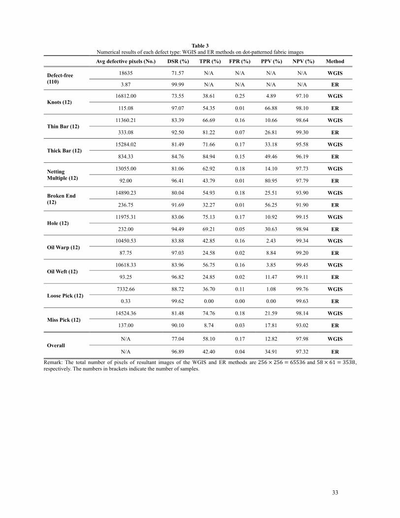
The detailed measurement metrics are obtained in the second step. Here, the ER method

obtains overall results of 96.89% DSR, 42.40% TPR, 0.04% FPR, 34.91% PPV and 97.32%

NPV for the dot-patterned fabric (Table 3), whereas the WGIS method generates overall results

of 77.04% DSR, 58.10% TPR, 0.17% FPR, 12.82% PPV and 97.98% NPV. The higher value

of PPV means that the ER method is more accurate when detecting defective regions, and the

lower values of FPR and NPV mean that the method is more accurate when detecting defect-

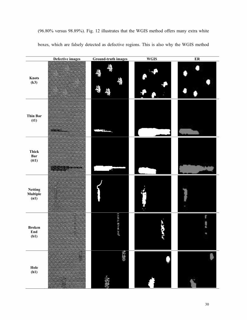
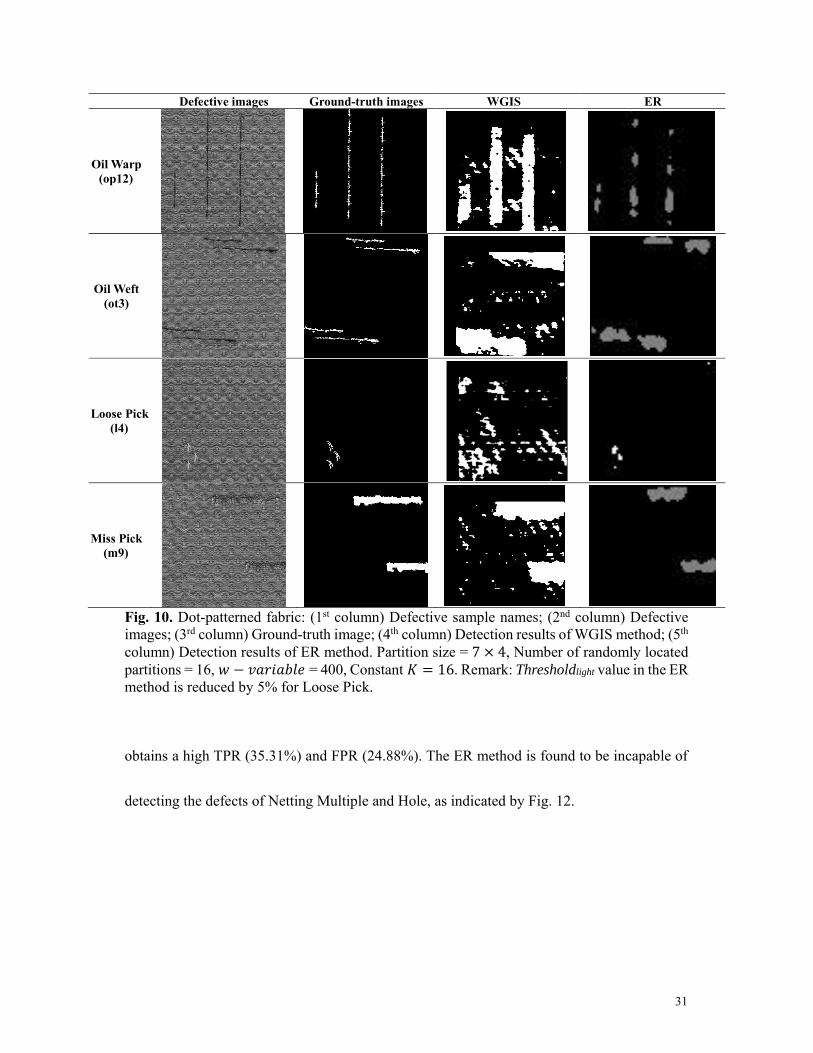
free regions. A higher DSR means better overall performance in detection. Fig. 10 depicts the

detection results of the WGIS and ER methods compared with the ground-truth images. The

ER method detects the light defect, Knots (first row) and Loose Pick (ninth row), more

accurately than the WGIS method. For the dark defects, i.e., Thin Bar, Thick Bar, Netting

Multiple, Broken End, Hole, Oil Warp, Oil Weft and Miss Pick, the ER method performs better

than the WGIS method with more accurate locations and more finely detected defect shapes.

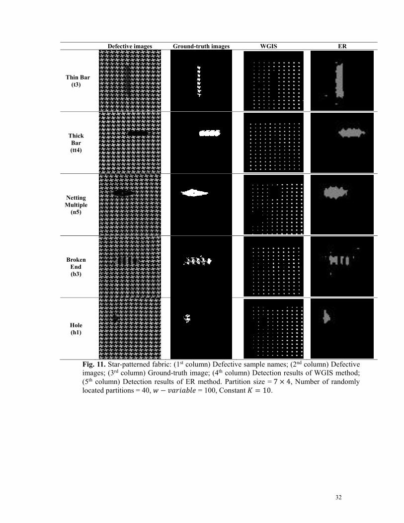
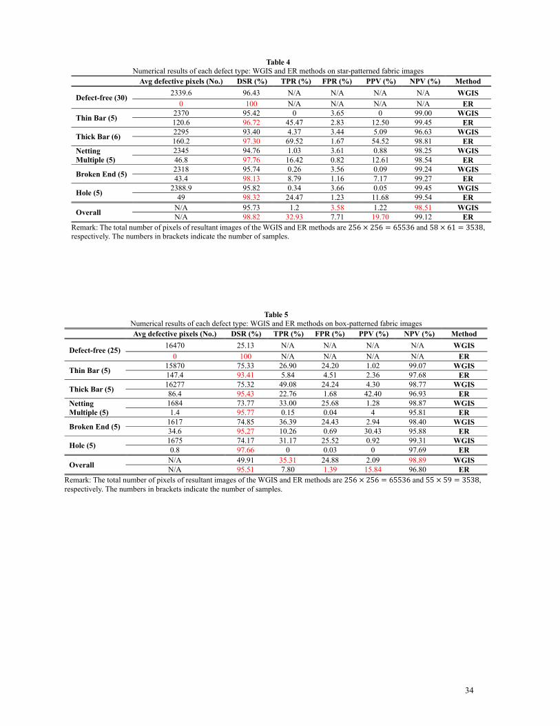
From Table 4 of the star-patterned fabric, the ER method shows better overall results

than the WGIS method in the metrics of DSR (98.82% versus 95.73%), TPR (32.93% versus

1.2%) and PPV (19.70% versus 1.22%) but poorer results for FPR (7.71% versus 3.58%) and

NPV (99.12% versus 98.51%). In Fig. 11, the WGIS method only provides white dots, which

are not a satisfactory visualised result, compared with the ER method. Table 5 shows the results

from the box-patterned fabric, in which the ER method shows higher rates than the WGIS

method in the overall results of DSR (95.51% versus 49.91%) and PPV (15.84% versus 2.09%)

and lower rates for TPR (7.80% versus 35.31%), FPR (1.39% versus 24.88%) and NPV

30

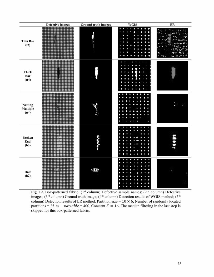
(96.80% versus 98.89%). Fig. 12 illustrates that the WGIS method offers many extra white

boxes, which are falsely detected as defective regions. This is also why the WGIS method

Defective images Ground-truth images WGIS ER

Knots (k3)

Thin Bar (t1)

Thick Bar (tt1)

Netting Multiple

(n1)

Broken End (b1)

Hole (h1)

31

obtains a high TPR (35.31%) and FPR (24.88%). The ER method is found to be incapable of

detecting the defects of Netting Multiple and Hole, as indicated by Fig. 12.

Defective images Ground-truth images WGIS ER

Oil Warp (op12)

Oil Weft (ot3)

Loose Pick (l4)

Miss Pick (m9)

Fig. 10. Dot-patterned fabric: (1st column) Defective sample names; (2nd column) Defective images; (3rd column) Ground-truth image; (4th column) Detection results of WGIS method; (5th column) Detection results of ER method. Partition size = 7 × 4, Number of randomly located partitions = 16, − = 400, Constant = 16. Remark: Thresholdlight value in the ER method is reduced by 5% for Loose Pick.

32

Defective images Ground-truth images WGIS ER

Thin Bar (t3)

Thick Bar (tt4)

Netting Multiple

(n5)

Broken End (b3)

Hole (h1)

Fig. 11. Star-patterned fabric: (1st column) Defective sample names; (2nd column) Defective images; (3rd column) Ground-truth image; (4th column) Detection results of WGIS method; (5th column) Detection results of ER method. Partition size = 7 × 4, Number of randomly located partitions = 40, − = 100, Constant = 10.

33

Table 3 Numerical results of each defect type: WGIS and ER methods on dot-patterned fabric images

Avg defective pixels (No.) DSR (%) TPR (%) FPR (%) PPV (%) NPV (%) Method

Defect-free (110)

18635 71.57 N/A N/A N/A N/A WGIS

3.87 99.99 N/A N/A N/A N/A ER

Knots (12) 16812.00 73.55 38.61 0.25 4.89 97.10 WGIS

115.08 97.07 54.35 0.01 66.88 98.10 ER

Thin Bar (12) 11360.21 83.39 66.69 0.16 10.66 98.64 WGIS

333.08 92.50 81.22 0.07 26.81 99.30 ER

Thick Bar (12) 15284.02 81.49 71.66 0.17 33.18 95.58 WGIS

834.33 84.76 84.94 0.15 49.46 96.19 ER

Netting Multiple (12)

13055.00 81.06 62.92 0.18 14.10 97.73 WGIS

92.00 96.41 43.79 0.01 80.95 97.79 ER

Broken End (12)

14890.23 80.04 54.93 0.18 25.51 93.90 WGIS

236.75 91.69 32.27 0.01 56.25 91.90 ER

Hole (12) 11975.31 83.06 75.13 0.17 10.92 99.15 WGIS

232.00 94.49 69.21 0.05 30.63 98.94 ER

Oil Warp (12) 10450.53 83.88 42.85 0.16 2.43 99.34 WGIS

87.75 97.03 24.58 0.02 8.84 99.20 ER

Oil Weft (12) 10618.33 83.96 56.75 0.16 3.85 99.45 WGIS

93.25 96.82 24.85 0.02 11.47 99.11 ER

Loose Pick (12) 7332.66 88.72 36.70 0.11 1.08 99.76 WGIS

0.33 99.62 0.00 0.00 0.00 99.63 ER

Miss Pick (12) 14524.36 81.48 74.76 0.18 21.59 98.14 WGIS

137.00 90.10 8.74 0.03 17.81 93.02 ER

Overall N/A 77.04 58.10 0.17 12.82 97.98 WGIS

N/A 96.89 42.40 0.04 34.91 97.32 ER

Remark: The total number of pixels of resultant images of the WGIS and ER methods are 256 × 256 = 65536 and 58 × 61 = 3538 , respectively. The numbers in brackets indicate the number of samples.

34

Table 4 Numerical results of each defect type: WGIS and ER methods on star-patterned fabric images

Avg defective pixels (No.) DSR (%) TPR (%) FPR (%) PPV (%) NPV (%) Method

Defect-free (30) 2339.6 96.43 N/A N/A N/A N/A WGIS 0 100 N/A N/A N/A N/A ER

Thin Bar (5) 2370 95.42 0 3.65 0 99.00 WGIS120.6 96.72 45.47 2.83 12.50 99.45 ER

Thick Bar (6) 2295 93.40 4.37 3.44 5.09 96.63 WGIS160.2 97.30 69.52 1.67 54.52 98.81 ER

Netting Multiple (5)

2345 94.76 1.03 3.61 0.88 98.25 WGIS46.8 97.76 16.42 0.82 12.61 98.54 ER

Broken End (5) 2318 95.74 0.26 3.56 0.09 99.24 WGIS43.4 98.13 8.79 1.16 7.17 99.27 ER

Hole (5) 2388.9 95.82 0.34 3.66 0.05 99.45 WGIS 49 98.32 24.47 1.23 11.68 99.54 ER

Overall N/A 95.73 1.2 3.58 1.22 98.51 WGIS N/A 98.82 32.93 7.71 19.70 99.12 ER

Remark: The total number of pixels of resultant images of the WGIS and ER methods are 256 × 256 = 65536 and 58 × 61 = 3538, respectively. The numbers in brackets indicate the number of samples.

Table 5 Numerical results of each defect type: WGIS and ER methods on box-patterned fabric images

Avg defective pixels (No.) DSR (%) TPR (%) FPR (%) PPV (%) NPV (%) Method

Defect-free (25) 16470 25.13 N/A N/A N/A N/A WGIS 0 100 N/A N/A N/A N/A ER

Thin Bar (5) 15870 75.33 26.90 24.20 1.02 99.07 WGIS147.4 93.41 5.84 4.51 2.36 97.68 ER

Thick Bar (5) 16277 75.32 49.08 24.24 4.30 98.77 WGIS86.4 95.43 22.76 1.68 42.40 96.93 ER

Netting Multiple (5)

1684 73.77 33.00 25.68 1.28 98.87 WGIS1.4 95.77 0.15 0.04 4 95.81 ER

Broken End (5) 1617 74.85 36.39 24.43 2.94 98.40 WGIS34.6 95.27 10.26 0.69 30.43 95.88 ER

Hole (5) 1675 74.17 31.17 25.52 0.92 99.31 WGIS 0.8 97.66 0 0.03 0 97.69 ER

Overall N/A 49.91 35.31 24.88 2.09 98.89 WGIS N/A 95.51 7.80 1.39 15.84 96.80 ER

Remark: The total number of pixels of resultant images of the WGIS and ER methods are 256 × 256 = 65536 and 55 × 59 = 3538, respectively. The numbers in brackets indicate the number of samples.

35

Defective images Ground-truth images WGIS ER

Thin Bar (t2)

Thick Bar (tt4)

Netting Multiple

(n4)

Broken End (b3)

Hole (h2)

Fig. 12. Box-patterned fabric: (1st column) Defective sample names; (2nd column) Defective images; (3rd column) Ground-truth image; (4th column) Detection results of WGIS method; (5th column) Detection results of ER method. Partition size = 10 × 6, Number of randomly located partitions = 25. − = 400, Constant = 16. The median filtering in the last step is skipped for this box-patterned fabric.

36

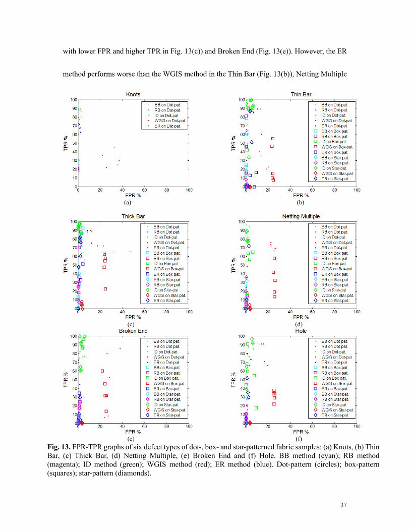
b) TPR-FPR graphs with optimised parameters

A further detailed comparison with TPR-FPR graphs [22] between the BB, RB, ID,

WGIS and ER methods is shown in Fig. 13. All methods were evaluated on the dot-, star- and

box-patterned fabric databases in [21]. Similar to that in an ROC graph, a point located closer

to the top left corner of the TPR-FPR graphs is regarded as an optimised result. The TPR-FPR

graphs are formulated by the TPR and FPR values of each defective sample of the dot-, star-

and box-patterned fabrics by the BB, RB, ID, WGIS and ER methods. This TPR-FPR graph

can help to evaluate how each method performs on each particular defect type. Only dot-

patterned fabric has the Knots defect. The blue dots in Fig. 13(a) clearly show that the TPR-

FPR points of the ER method are close to the top left corner of the graph than those of the BB,

RB and WGIS methods. For the dot-patterned fabric, the ER method obviously outperforms

the BB, RB and WGIS methods for each defect type. In regard to the star-patterned fabric, the

ER method (blue diamonds) demonstrates superiority in the Thin Bar (Fig. 13(b)), Thick Bar

(Fig. 13(c)), Netting Multiple (Fig. 13(d)), Broken End (Fig. 13(e)) and Hole (Fig. 13(f))

defects. Most of the TPR-FPR points of the BB, RB and WGIS methods, shown as cyan,

magenta and red diamonds, are located at the bottom left corner of the plots, indicating both

low TPR and low FPR. This is also due to the complete darkness in the final resultant images

once all noise is removed. For the box-patterned fabric, most methods do not performs as well

as in the previous two patterned fabrics. The ER method performs slightly better than the WGIS

method and much better than the BB and RB methods in the Thick bar defect (ER: blue boxes

37

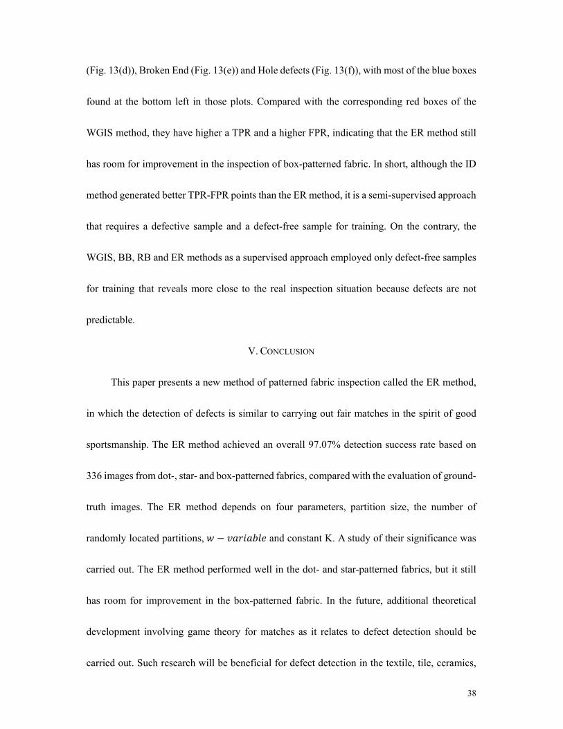
with lower FPR and higher TPR in Fig. 13(c)) and Broken End (Fig. 13(e)). However, the ER

method performs worse than the WGIS method in the Thin Bar (Fig. 13(b)), Netting Multiple

(a)

(b)

(c)

(d)

(e)

(f)

Fig. 13. FPR-TPR graphs of six defect types of dot-, box- and star-patterned fabric samples: (a) Knots, (b) Thin Bar, (c) Thick Bar, (d) Netting Multiple, (e) Broken End and (f) Hole. BB method (cyan); RB method (magenta); ID method (green); WGIS method (red); ER method (blue). Dot-pattern (circles); box-pattern (squares); star-pattern (diamonds).

38

(Fig. 13(d)), Broken End (Fig. 13(e)) and Hole defects (Fig. 13(f)), with most of the blue boxes

found at the bottom left in those plots. Compared with the corresponding red boxes of the

WGIS method, they have higher a TPR and a higher FPR, indicating that the ER method still

has room for improvement in the inspection of box-patterned fabric. In short, although the ID

method generated better TPR-FPR points than the ER method, it is a semi-supervised approach

that requires a defective sample and a defect-free sample for training. On the contrary, the

WGIS, BB, RB and ER methods as a supervised approach employed only defect-free samples

for training that reveals more close to the real inspection situation because defects are not

predictable.

V. CONCLUSION

This paper presents a new method of patterned fabric inspection called the ER method,

in which the detection of defects is similar to carrying out fair matches in the spirit of good

sportsmanship. The ER method achieved an overall 97.07% detection success rate based on

336 images from dot-, star- and box-patterned fabrics, compared with the evaluation of ground-

truth images. The ER method depends on four parameters, partition size, the number of

randomly located partitions, − and constant K. A study of their significance was

carried out. The ER method performed well in the dot- and star-patterned fabrics, but it still

has room for improvement in the box-patterned fabric. In the future, additional theoretical

development involving game theory for matches as it relates to defect detection should be

carried out. Such research will be beneficial for defect detection in the textile, tile, ceramics,

39

wallpaper, aircraft window and printed circuit board industries and for the latest three-

dimensional printing technologies.

Acknowledgements

The second author was supported by a Hong Kong Baptist University Faculty Research

Grant/12-13/075.

40

APPENDIX

Algorithm 1 Threshold acquisition from a score matrix Require: k defect-free image. ( = 5 in our case.) 1: for each defect-free image R 2: perform level 2 Haar wavelet transformation 3: end 4: output: k level 2 Haar wavelet transformed defect-free image, of size × 5: for each 6: select a golden partition of size m × n, 7: end 8: for each 9: slide on each pixel along each row p on , x ∈ M 10: for y = 1: N 11: calculate , in each match 12: end 13: end 14: output: a score matrix = { , } 15: for each 16: obtain the maximum and minimum values, ( ) = , ( ) = 17: end 18: take average of all and 19: output: Threshold = and Threshold =

Algorithm 2 Training stage of the ER method Require: k Elo reference matrix w.r.t. k level 2 Harr wavelet transformed defect-free

image, . ( = 5 in our case) 1: for each 2: slide on each pixel along each row x, x ∈ M and obtain a m × n partition . 3: for each . 4: randomly select r partitions to have matches with . 5: match’s win/tie/loss determined by {Threshold , Threshold } in Algorithm

1: Threshold Acquisition from a Score Matrix 6: update the corresponding element on 7: end 8: end 9: output: updated Elo matrix 10: for each 11: obtain the maximum and minimum value 12: end 13: output: Threshold = and Threshold =

41

REFERENCES

[1] H.Y.T. Ngan, G.K.H. Pang and N.H.C. Yung, “Automated Fabric Defect Detection – A Review,” Image and Vision Computing, vol. 29, no. 7, pp. 442-458, 2011.

[2] H.Y.T. Ngan, G.K.H. Pang and N.H.C. Yung, “Motif-based Defect Detection for Patterned Fabric,” Pattern Recognition, vol. 41, no. 6, pp. 1878-1894, 2008. [3] D-M. Tsai, M-C. Chen, W-C. Li and W-Y. Chiu, “A Fast Regularity Measure for Surface

Defect Detection,” Machine and Vision Application, vol. 23, pp. 869-886, 2012. [4] H-G. Bu, J. Wang and X-B. Huang, “Fabric Defect Detection based on Multiple Fractal

Features and Support Vector Data Description,” Engineering Applications of Artificial Intelligence, vol. 22, pp. 224-235, 2009.

[5] K.L. Mak, P. Peng, K.F.C. Yiu, “Fabric Defect Detection using Morphological Filters,” Image and Vision Computing, vol. 27, pp. 1585-1592, 2009.

[6] M.A. Aziz, A.S. Hagga and M.S. Sayed, “Fabric Defect Detection Algorithm using Morphological Processing and DCT,” Proc. IEEE ICCSPA, pp. 1-4, 2013.

[7] C. H. Chan and G.K.H. Pang., “Fabric Defect Detection by Fourier Analysis,” IEEE Trans. Industry Applications, vol.36, no.5, Sept/Oct 2000.

[8] D. Aiger and H. Talbot, “The Phase Only Transform for Unsupervised Surface Defect Detection,” Proc. IEEE CVPR, pp. 295-302, 2010.

[9] D. Schneider, T. Holtermann, F. Neumann, A. Hehl, T. Aach and T. Gries, “A Vision Based System for High Precision Online Fabric Defect Detection,” Proc. IEEE ICIEA, pp. 1494-1499, 2012.

[10] A. Kumar and G.K.H. Pang, “Defect Detection in Textured Materials Using Gabor Filters,” IEEE Trans. Industry Applications, vol. 38, no.2, pp. 425-440, 2002.

[11] X.Z. Yang, G.K.H. Pang and N.H.C. Yung, “Discriminative fabric defect detection using directional wavelets,” Optical Engineering, vol. 41, no. 12, pp. 3116-3126, 2002.

[12] X.Z. Yang, G.K.H. Pang and N.H.C. Yung, “Discriminative training approaches to fabric defect classification based on wavelet transform,” Pattern Recognition, vol. 37, issue 5, pp. 889-899, 2004.

[13] H. Zuo, Y. Wang, X. Yang and X. Wang, “Fabric Defect Detection Based on Texture Enhancement,” Proc. IEEE CISP, pp. 876-880, 2012.

[14] F.S. Cohen, Z.G. Fan, S. Attali, “Automated Inspection of Textile Fabric using Textural Models,” IEEE Trans. Pattern Analysis & Machine Intelligence, vol. 13, no. 8, pp. 803–808, Aug 1991.

[15] J. Zhou, D. Semenovich, A. Sowmya and J. Wang, “Sparse Dictionary Reconstruction for Textile Defect Detection,” Proc. IEEE ICMLA, pp. 21-26, 2012.

[16] Z. Kang, C. Yuan and Q. Yang, “The Fabric Defect Detection Technology Based on Wavelet Transform and Neural Network Convergence,” Proc. IEEE ICIA, pp. 597-601, 2013.

[17] A. Bodnarova, M. Bennamoun, and K.K. Kubik, “Defect Defection in Textile Materials Based on Aspects on the HVS,” Proc. IEEE Int'l Conf. SMC, pp. 4423–4428, 1998.

[18] H.Y.T. Ngan, G.K.H. Pang, S.P. Yung and M.K. Ng, “Wavelet based methods on Patterned Fabric Defect Detection,” Pattern Recognition, vol. 38, issue 4, pp. 559-576, 2005.

[19] C.J. Kuo, and T. Su, “Gray relational analysis for recognizing fabric defects,” Textile Research Journal, vol. 73, no. 5, pp. 461–465, 2003.

[20] H.Y.T. Ngan and G.K.H. Pang, “Novel Method for Patterned Fabric Inspection using Bollinger Bands,” Optical Engineering, vol. 45, no. 8, Aug, 2006.

[21] H.Y.T. Ngan and G.K.H. Pang, “Regularity Analysis for Patterned Texture Inspection,” IEEE Trans. Automation Science & Engineering, vol. 6, no. 1, pp. 131-144, 2009.

42

[22] M.K. Ng, H.Y.T. Ngan, X. Yuan and W. Zhang, “Patterned Fabric Inspection and Visualization by the Method of Image Decomposition,” IEEE Trans. Automation Science & Engineering, vol. 11, no. 3, pp. 943-947, 2014.

[23] A. E. Elo, The Rating of Chess Players, Past and Present, New York: Arco, 1978. [24] P.C.H. Albers and H. de Varies, “Elo-rating as a Tool in the Sequential Estimation of

Dominance Strengths”, Animal Behaviour, vol. 61, pp. 489-490, 2001. [25] H.Y.T. Ngan, G.K.H. Pang and N.H.C. Yung, “Performance Evaluation for Motif-based

Patterned Texture Defect Detection,” IEEE Trans. Automation Science & Engineering, vol. 7, no. 1, pp. 58-72, 2010.

[26] Y. Li and X. Di, “Fabric Defect Detection using Wavelet Decomposition,” Proc. IEEE CECNet, pp. 308-311, 2013.

[27] G. Stubl, J-L. Bouchot, P. Haslinger and B. Moser, “Discrepancy Norm as Fitness Function for Defect Detection on Regularly Textured Surfaces,” LNCS, vol. 7476, pp. 428-437, 2012.

[28] J.L. Raheja, S. Kumar and A. Chaudhary, “Fabric Defect Detection based on GLCM and Gabor filter: A Comparison,” Optik – Int’l J. Light and Electron Optics, vol. 124, no. 23, pp. 6469-6474, 2013.

[29] M. Li, Z. Deng and L. Wang, “Defect Detection of Patterned Fabric by Spectral Estimation Technique and Rough Set Classifier,” Proc. IEEE GCIS, pp. 190-194, 2013.

43

VITAE COLIN S.C. TSANG is an undergraduate year-4 student in mathematics at Hong Kong Baptist University, China. He is supposed to obtain B.Sc. (Hons.) in mathematical science in 2015. He likes sport matches in daily life. His current research interests include surface defect detection, pattern recognition and image processing. HENRY Y.T. NGAN obtained a B.Sc. degree in mathematics in 2001, a M. Phil. Degree in 2005 and a Ph.D. degree in 2008 in electrical and electronic engineering at The University of Hong Kong (HKU), China. He is currently a research assistant professor at the Department of Mathematics, Hong Kong Baptist University. Previously, he worked in the Laboratory for Intelligent Transportation Systems Research, HKU in 2010-2012 and the IARL, HKU in 2002-2008. He held visiting positions in Electric & Electrical Engineering, the University of Sheffield, U.K. in 2012-2014, the CCIL, NEC, Japan and the Carnegie Mellon CyLab, Carnegie Mellon University, U.S. at Kobe, Japan in 2008-2009, and at the IAL, the University of British Columbia, Canada in 2006. He carried out industrial and consultancy projects for Hong Kong ASTRI and CFM Management Company Ltd., H.K. in 2010-2011. His current research interests include pattern recognition application on anomalies detection, large-scale data analysis, social signal processing, visual surveillance, intelligent transportation systems and medical imaging. He serves as a reviewer for many international conferences and journals. He is a senior member of the IEEE and a member of the ACM and the IET. GRANTHAM K.H. PANG obtained his Ph.D. degree from the University of Cambridge in 1986. He was with the Department of Electrical and Computer Engineering, University of Waterloo, Canada, from 1986 to 1996. After that, he joined the Department of Electrical and Electronic Engineering at The University of Hong Kong as an Associate Professor. He has published more than160 technical papers and has authored or co-authored six books. He has also obtained five U.S. patents. His research interests include machine vision for surface defect detection, video surveillance, expert systems for control system design, intelligent control and intelligent transportation systems. Dr. Pang is a Chartered Electrical Engineer, and a member of the IET, HKIE as well as a Senior Member of IEEE. Dr. Pang has acted as consultant to many local and international companies.