EXTRACTION OF SIGNALS IN THE PRESENCE OF

STRONG NOISE: CONCEPTS AND EXAMPLES

RALPH V. BALTZInstitut fur Theorie der Kondensierten Materie

Universitat Karlsruhe, D–76128 Karlsruhe, Germany ∗

INTERNATIONAL SCHOOL OF ATOMIC AND MOLECULAR SPECTROSCOPYFrontier Developments in Optics and SpectroscopyEttore Majorana Center for Scientific Culture, Erice, Sicily, June 17 – July 2, 2007Director: B. Di Bartolo, Boston College, USA

1. Introduction

In experimental physics, communication electronics and other technicaldisciplines one is often faced with the challenge of detecting weak signalss(t) which are buried under noise n(t). Assuming a linear superposition,the total signal is

f(t) = s(t) + n(t), S/N = 10 log(Ps

Pn) dB. (1)

S/N denotes the signal to noise ratio and Ps, Pn, respectively, are the powerof the signal and noise in the bandwidth of the detector. Here, noise is shortfor all types of broadband disturbances masking the information which iscontained in s(t).

Depending on the character of the signal the human ear is capable toextract signals which are 6dB under the noise level. Good quality broadcastrequires at least S/N= +20dB whereas experiments often struggle withS/N= −40dB or less.

In this article, signals are always understood as (multicomponent) func-tions of time. Signal processing with respect to spatial variables is the fieldof image–processing and pattern–recognition.

The plan of this contribution is twofold. In chapters 2-4, general con-cepts of signal processing and statistical properties of noise are reviewed,whereas chapt. 5 gives a selection of examples with sketchy solutions. Chap-ter 6 contains some closing remarks on Quantum Noise. For general refer-ences see Refs.[1](a-c). The only book which – to my knowledge – conformswith the title of this report is an old book by Wainstein and Zubakov[2]with emphasis on radar signals.

∗ http://www.tkm.uni-karlsruhe.de/personal/baltz/

2

Figure 1. Huygens signal received at the Green Bank Telescope (GBT), USA[4](c).

2. Signals

A recent spectacular example of weak signal detection is the direct receptionof the Huygens signal by some very large radio telescopes[3](a,b). Due to anerror in the configuration of the receiver on the Cassini relay the completedata of the Huygens Doppler wind–experiment during descend on Saturn’smoon Titan would otherwise be lost[4](a,b). (For some technical details seethe JPL–report[5] and appendix A). Refs.[6](a,b) provide two additionalexamples of weak–signal–detection with amateur equipment:– radio communication via reflections from the moon (power < 1kW),– detection of a Mars orbiter relay on 437MHz (1W, isotropic radiation).

The natural mathematical basis for the representation and processingof signals is the complex Fourier–transformation (FT)[7](a),1

FT: f(t) =

∫ ∞

−∞F (ω) e−iωt dω

2π, F (ω) =

∫ ∞

−∞f(t) eiωt dt. (2)

In practice, FT is always performed over finite time– and frequency–intervals.To remove artefacts from the ends of the time–integration interval a window–function w(t) is used which smoothly tends to zero near the endpoints. Aconvenient window–function is the Hamming–window [7](b)

wH(t) =1

2

(

1 + cosπt

T

)

θ(T 2 − t2).

Moreover, a time and frequency dependent windowed-FT can be definedfrom which – remarkably – the complete signal f(t) can be reconstructed

F (ω, τ) =

∫ ∞

−∞f(t′)w(t′ − τ) eiωt′ dt′, (3)

1 Fourier–transformed functions are denoted by capitals, if suitable.

3

x n s

1 h¾ -

Figure 2. Screen shot of slow speed telegraphy signals (60s per dot) on 137 kHzreceived in north Germany by sliding FT. Upper trace: station WD2XNS (east coastUSA, radiated power ≈ 1 W) sending Morse–Code “xns”. Horizontal axis: time, verticalaxis: frequency (total span ≈ 2 Hz). From Ref.[8](a).

j

jf(t )

0 5 10 15 20

0.2

0.4

0.6

0.8

1

1.2

N=20t=0.25∆

a)

0

F(ωk)2

∆ω=2π/5

k

0 5 10 15 20

0.4

0.6

−5−10

0.8

1

0.2

b)

Figure 3. Discrete Fourier–Transformation.

f(t) =1

w(0)

∫ ∞

−∞F (ω, t) e−iωt dω

2π, (4)

F (ω) =1

W

∫ ∞

−∞F (ω, τ) dτ , W =

∫ ∞

−∞w(τ)dτ. (5)

Fig. 2 diplays an example of a time dependent FT which is used inamateur radio to detect very weak signals transmitted on 137 kHz acrossthe Atlantic[8](a-c).

Today, signal processing is mainly numerically done, first by– Analogue–Digital Conversion (ADC): f(t) → fj = f(tj), tj = j∆t,

where ∆t is the sampling–time and j = 0, 1, . . . , (N − 1).– Then, FT is performed in discretized form (DFT) for both f(t) and F (ω),

DFT: fj =N−1∑

k=0

Fk e−i 2π

Njk, Fk =

1

N

N−1∑

j=0

fj ei 2π

Njk. (6)

Time span: T = N∆t. Frequency resolution: ∆ω = 2π/T , ωk = k∆ω.– Technically, FT is performed using standard Fast–Fourier routines[9].

4

t0t0

f

t t

xinput output

h(t,t’)

Figure 4. Block diagram of a linear system transforming f(t) into x(t).

fj as well as Fk are periodic functions of j and k (mod N) which maycause “aliasing problems”, see Fig. 3. Very often, a symmetric form of thek–periodicity interval with respect to k = 0 is used (as in solid state theory):|ω| < Ω = π/∆t (Nyquist–rate).

Remarkably, the analogue signal f(t) can be perfectly reconstructedfrom the discretized signal fj provided f(t) is band–limited [10].

Bernstein–Theorem:

if: fj = f(j∆t), j = 0, 1, . . . N − 1, and

F (ω) ≡ 0 for |ω| > Ω, Ω = π/∆t,

then: f(t) =N−1∑

j=0

fjsinc(Ωt − jπ), sinc(x) =sin(x)

x. (∗)

Support of f(t): extends from −∞ to ∞,derivatives: exist to all orders.

In principle, the Bernstein–result (∗) could be used for Digital–Analogue–

Conversion (DAC). In practice, however, DAC is performed holding f(t) =fj =const in the time–interval tj ≤ t < tj+1 (”histogram”) with subsequentsmoothening by an analogue low pass filter (RC–circuit).

3. Linear Systems

A linear System (LS) – as sketched in Fig. 3 – is a device which linearlytransforms an input signal f(t) into an output x(t),

Linear System: x(t) =

∫ ∞

−∞h(t, t′) f(t′) dt′. (7)

h(t, t′) is called the (impulse) Response Function, system–function or just“filter”. 2

2 f(t), x(t), h(t, t′) may have several components or may be fields.

5

H(ω)

Re H Im H

h(t)

ωt0 2 4 6−2−4

−0.25

0

0.25

0.5

0.75

1

0−2−4 2 4 6

−0.2

0

0.2

0.4

0.6

0.8

1 a) b)

Figure 5. Ideal low–pass filter (full lines) and relaxator (dashed/dotted lines).

Basic properties are[1]:

– time–invariance: h(t, t′) = h(t − t′),

– TI+causality: h(t − t′) ≡ 0, t′ > t,

– in ω–space: X(ω) = H(ω)F (ω),

– analyticity: H(ω) analytic function of complex ω for Imω > 0(time–invariant causal systems).

Examples:

a) unit–system: h(t) = δ(t), H(ω) = 1,

b) delay–line: h(t) = δ(t − T ), H(ω) = eiωT,

c) relaxator: h(t) = e−γt Θ(t), H(ω) =1

γ − iω,

d) ideal low–pass: h(t) =Ω

πsinc(Ωt), H(ω) = Θ(Ω2 − ω2),

(a) (b) (c)

Figure 6. Mechanical filter Telefunken FE 21 [14 coupled, torsional steel resonators;conversion of the electric signal into mechanical vibrations and back to an electricalsignal]. (a) H(ω), (b) phase Φ(ω) of H(ω), (c) pulse delay time τ = ∂Φ

∂ω. From Ref[11].

6

T T

f(t)

t

Figure 7. Three members of a statistical ensemble of a random signal.

Fig. 5 displays the system functions for c) and d). A relaxator actsas a Low–Pass–Filter (LPF) which can be realized as a RC–circuit (“in-tegrator”). Example (d) refers to an ideal LPF. As h(t) 6= 0 for t < 0,such a filter is acausal and can be only realized as a digital filter. Fig. 6shows the characteristics of a mechanical filter which was used in high–endcommercial and military short–wave reveivers.

Clearly, extraction of weak, but spectrally narrow signals, can be suc-cessfully done by reducing the bandwidth of the receiver (“filtering”), seeFigs. 1,2.

Today, signal processing is mainly numerically performed by first digi-tizing the signal by an ADC, FT, filtering, inverse FT, and DAC to back tothe time–domain. Apparently, digital filters may (mathematically) violatecausality.3 Nevertheless, digital filters can be much more powerful thananalogue filters.

4. Noise

4.1. STOCHASTIC DESCRIPTION

There are signals which are so irregular (“erratic”) that only a probabilisticdescription is possible. But noise is not always a hindrance of signal detec-tion, in some cases, the noise itself is the signal, e.g., in the Hanbury–Brown

& Twiss effect [12] or studies on electron kinetics[13].

Basic rules are[14]:

– time average: x(t) = limT→∞

1

2T

∫ T

−Tx(t + t′) dt′,

3 Digitizing the analogue signal during time T , data–storage, FT, etc. needs a finitetime so that the analogue output can never appear before the input signal ended.

7

n=50.1

0.2

0 2 4 6 8 10 12 14

n

a)P(n)

x=2∆

0.1

0.2

0 2 4 6 8 10 12 14

b)x=5

x

P(x)

x=3∆

Figure 8. a) Poissonian and b) Gaussian–distributions[14](a,b).

– ensemble average: 〈x(t)〉 = limN→∞

1

N

N∑

k=1

xk(t),

– ergodicity (+stat.): 〈x(t)〉 = x(t) (= 0),

– probability dist.: P (x, t) > 0,∫

P (x, t) dx = 1,

〈xk(t)〉 =

∫

P (x, t)xk dx, k = 0, 1, 2, . . .

– deterministic signal: P (x, t) = δ(x − ξ(t)), ξ(t) prescribed function.

A complete description of a random process x(t) requires the knowledge ofthe probability of the whole process, i.e. P [x(t)]. This is equivalent to theknowledge of P (x; t), joint probability P (x1, x2; t1, t2), etc.

Central limit theorem:If x is the sum of many independent, random variables then P (x) becomesa Gaussian (irrespective of the statistics of the individual variables)

PG(x) =1√2πσ

e−(x−x)2

2σ , σ = (∆x)2.

Poissonian distribution:The Poissonian PP(n) is the limiting case (p ¿ 1, n ¿ N) of a Binomial

distribution. The probability that an event characterized by probability poccurs n times in N trials reads

PB(n) =

(

N

n

)

pn (1 − p)N−n → PP(n) = e−n nn

n!, n = pN.

8

4.2. CORRELATION FUNCTIONS

In addition to the probability distribution functions a second set, namedcorrelation functions will be useful[14](a,b)

Cff(t1, t2) = f(t + t1) f(t + t2) =

∫ ∫

P (f1, f2; t1, t2) f1 f2 df1 df2. (8)

Basic properties are[14]:

– steady state: Cff(t1, t2) = Cff(|t1 − t2|) =

∫

Cff(ω) e−iω(t1−t2) dω

2π,

– inequality: |Cff(t)| < Cff(t = 0), t = t1 − t2,

– quadratic average: 〈[f(t)]2〉 =∫

Cff(ω) dω2π ,

– power spectrum: Cff(ω) = 12T |F (ω)|2 > 0,

– white noise: Cff(ω) =const, Cff(t) ∝ δ(t).

Wiener–Khinchine–Th: Cff(ω) =1

2T|F (ω)|2 > 0. (9)

F (ω) of a stationary, random process f(t) may not exist. This is circum-vented by using a time cut–off, i.e. setting f(t) ≡ 0 for |t| > T andperforming the limit T → ∞ at the end.4

Filtering of a random signal:Filtering f(t) with correlation function Cff(ω) leads to an output signalwith changed correlations

Filtered Noise: Cxx(ω) = |H(ω)|2 Cff(ω). (10)

In particular, filtering of white noise creates correlations of finite duration.Numerous examples of student experiments on noise and correlation canbe found in the American Journal of Physics, e.g. Refs.[15](a-c).

An example of an apparatus to measure correlations of the electromag-netic field in the optical region is the Michelson interferometer, see Fig. 9.For a box–shaped intensity profile of total width ∆ω centered at ω0 > 0,the complex optical coherence function becomes

G(t2 − t1) = 〈E(−)(t2)E(+)(t1)〉 = I0∆ω

2e−iω0(t2−t1) sinc

(

∆ω(t2 − t1)

2

)

.

4 F (ω) implicitely depends on T but |F |2/T is well–defined for T → ∞.

9

M2

t1

t2

M

from

source

STM

to detector

a)

1

tcoh

ω0

t

ω0−

I (ω)=

ω

∆ωrmsE2

c)

b)

G(t)1

−1

Figure 9. (a) Principle of a Michelson interferometer to measure the correlations in theoptical electrical field, (b) filtered white noise, (c) coherence function.

E(±)(t) denote the positive/negative frequency components of the opticalelectrical field E(t) = E(+)(t) + E(−)(t), see any book on quantum optics orRef.[12].

4.3. SHOT NOISE

The thermionic current in a vacuum tube is not a smooth flow of electricity,but is subject to rapid and irregular fluctuations. These fluctuations, dis-covered by Schottky[16](a) (1918) and called by him “Schrot–Effekt” (smallshot–effect) are caused by the random emission of (single) electrons fromthe cathode and are made manifest by voltage or current fluctuations inany circuit to which the tube is connected. If each emitted electron reachesthe anode (saturation) within a neglectable transit time, the current willshow–up as delta–spikes with Poissonian statistics (during fixed time), seeFig. 10(c).

– fluctuating current: I(t) =∑

k

eδ(t − tk) = Idc + In, Idc = en,

– current corr. function: CII(t) = e2(∆n)2 δ(t), (∆n)2 = n,

– power spectrum: CII(ω) = ne2 = eIdc, (white noise).

A bandwidth of ∆ω contributes to the noise current (a factor 2 arises fromthe contributions at ±ω0)

Schottky–Formula: I2rms = 2eIdc ∆ν, ∆ν = ∆ω/(2π). (11)

10

Ua

C

R

U

Unoise

a

+

light+

I(t)

t

Idc

b) c)a)

Figure 10. (a) Vacuum tube, (b) vacuum photo–cell, (c) shot noise current.

Example:Idc = 1mA, ∆ν = 5kHz, ; Irms = 1.3nA, Urms = 13µV (at R = 10kΩ).

Z( )ωaU

a)

outCR

L

U

+

Uex

p2

/U2 th

x

0 1 2 3 4 5 6

2

4

6

8

10

12

14

16

18

20

b)

tungsten cathodex oxidized cathode

x

xxxxx

xxxxx

xx

xxxxxxxx

xx xx x x xx x x x x x x x x x

Frequency (KHz)

Figure 11. (a) Experimental set–up and (b) measured shot–noise power spectrum. Z(ω)is the impediance of the RCL circuit. The amplifier consisted of 5 tubes Western Electric101/102D, RC–coupled with Uout = 3 × 105Uin. Redrawn from Ref.[16](b)

Fig. 11(a) sketches Johnson’s experimental set–up[16](b) to measurethe spectral dependence of the shot–noise from a vacuum tube by using aLC–resonance circuit, where ω0 = 1/

√LC and

U2rms =

∫ ∞

−∞|Z(ω)|2CII(ω)

dω

2π=

eIdc

2C2

(

L

R+ RC

)

.

Note, Urms depends on the loss–resistance R, which had to be determinedfrom the resonance curve of each LC circuit.

Thermionic emission from oxidized cathodes is more efficient than frompure metallic cathodes but it is more noisy (“1/f” noise), see Fig.11(b).In Quantum optics, shot noise is caused by fluctuations of the detectedphotons, e.g. in a vacuum photo–cell.

11

a) b)

noise

R Lsource

resistorideal Rv

M

molecules

Figure 12. (a) Brownian motion of a particle in a fluid, (b) L–R circuit.

4.4. THERMAL NOISE (JOHNSON, NYQUIST, 1926)

The mechanism of noise–generation by a resistor at finite temperature T0 isanalogue to the Brownian motion of a heavy particle of mass M immersedin a fluid. The force of the molecules “pinging” on the Brownian particleconsists of two parts: a frictional force −γ′v and a stochastic force fst

which will be modelled by white noise. Remarkably, both parts are notindependent but related by the dissipation–fluctuation theorem[17](b).

– Brownian motion: Mv = ftotal = −γ′v + fst(t),

– velocity: V (ω) = 1M

1γ−iω Fst(ω), γ = γ′/M ,

– correlation function: Cvv(ω) = 12T |V (ω)|2 = |H(ω)|2 Cff(ω),

– white noise: Cff(ω) = 12T |F (ω)|2 = κ =const,

– equipartion theorem:M

2v2(t) =

M

2

∫

Cvv(ω)dω

2π=

1

2kBT0,

– diss.–fluct. theorem: κ = 2kBT0Mγ.

The corresponding result for the LR–circuit is obtained by translating v →I, M → L, γ → R/L, thus CUU(ω) = 2kBT0R. This leads to the famous

Nyquist–Formula: U2rms = 4kBT0R ∆ν. (12)

This result can be generalized to an arbitrary impediance by R → Re Z(ω).Note, the equivalent circuit diagram of a real resistor consists of an ideal(noise–free) resistor with resistance R and a noise source with correla-tion function CUU(ω) = 2kBT0R, see Fig. 12(b). Fig. 13 displays Johnsonsoriginal result.Example:R = 1MΩ, T0 = 300K, ∆ν = 5kHz, ; Urms ≈ 2.5µV.

12

Figure 13. Noise power U2rms/R generated by a resistor at temperature T0[17](a).

5. Examples of Signal Extraction from Noise

5.1. BOX–CAR INTEGRATOR

The Box–Car Integrator (BCI) improves the S/N ratio by

– gating the detection (time window ∆t),

– averaging over multiple pulses, S/N∼√

N ,e.g. N = 104 improves S/N by 20dB.

Beginning with t0 = 0, the “box–car” is shifted gradually to highervalues so that the full signal dependence of the signal is covered, see Fig. 14.Today, BCI’s are a standard tool in most physics laboratories.

Typical properties of commercially available instruments are

– integration time: ∆t = 2 . . . 15µs,

– number of samplings: N = 1 . . . 10000,

– trigger rate: dc. . . 20kHz.

5.2. LOCK–IN AMPLIFIER

In its most basic form a Lock–In Amplifier (LIA) is an instrument with dualcapability. It can recover signals in the presence of an overwhelming noisebackground or, alternatively, it can provide high resolution measurementsof relatively clean signals over several orders of magnitude and frequency.(Modern instruments even offer more than these two basic functions).

13

1 1 11 1.25 1.25 1.251.25 1.5 1.5 1.51.5 1.75 1.75 1.751.75 2 2 22

∆t ∆t ∆t∆t

t0 t0 t0 t0

t

x(t)

Figure 14. Principle of a Box–Car integrator.

x

Ref ϕ

Exp.

chopperto

outputLPFBPF

Figure 15. Principle of a Lock–In amplifier. (BPF/LPF: band–pass/low–pass filter).

The LIA (in common with most ac indicating instruments) provides a dcoutput proportional to the ac input signal. In this method, one modulates(or chops) the input signal at a frequency appreciably above the informationcarrying frequency of the signal, amplifies at the modulation–frequency, andthen synchronously demodulates this amplified output in order to recoverthe original signal information. The output of this phase sensitive detection

is proportional to

LIA: C(ϕ, T ) =1

T

∫ T

0f(t) sin(ωt + ϕ) dt. (13)

T denotes the integration time and ϕ is the relative phase between the(sinusoidally) modulated signal and the reference. Thus, the LIA operatesas an effective LPF with a bandwidth ≈ 1/T .

Introductory articles about the lock–in technique may be downloadedfrom the web–pages of several companies, e.g. Refs. [18](a). In addition,there are numerous articles published in the American Journal of Physicsabout the physics and technique of lock–in laboratory experiments, e.g.Refs.[18](b-d).

14

H( )ωH( )ω

S N

S

N

ω ω

b)a)

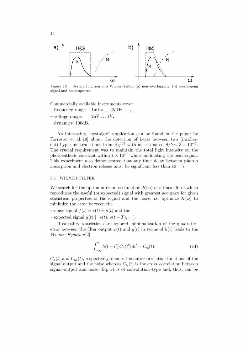
Figure 16. System function of a Wiener–Filter. (a) non–overlapping, (b) overlappingsignal and noise spectra.

Commercially available instruments cover

– frequency range: 1mHz . . . 2MHz . . . ,

– voltage range: 2nV . . . 1V,

– dynamics: 100dB.

An interesting “nostalgic” application can be found in the paper byForrester et al.[19] about the detection of beats between two (incoher-ent) hyperfine transitions from Hg202 with an estimated S/N∼ 3 × 10−5.The crucial requirement was to maintain the total light intensity on thephotocathode constant within 1 × 10−5 while modulating the beat–signal.This experiment also demonstrated that any time–delay between photonabsorption and electron release must be significant less than 10−10s.

5.3. WIENER–FILTER

We search for the optimum response function H(ω) of a linear filter whichreproduces the useful (or expected) signal with greatest accuracy for givenstatistical properties of the signal and the noise, i.e. optimize H(ω) tominimize the error between the

– noisy signal f(t) = s(t) + n(t) and the

– expected signal g(t) [=s(t), s(t − T ),. . . ].

If causality restrictions are ignored, minimalization of the quadratic–error between the filter output x(t) and g(t) in terms of h(t) leads to theWiener–Equation[2]

∫ ∞

−∞h(t − t′)Cff(t

′) dt′ = Cfg(t). (14)

Cff(t) and Cnn(t), respectively, denote the auto–correlation functions of thesignal output and the noise whereas Cfg(t) is the cross–correlation betweensignal–output and noise. Eq. 14 is of convolution–type and, thus, can be

15

x (t)0

h(t; λ)

on/off

f(t) x(t)

ε −update λFigure 17. Sketch of an adaptive filter. x0(t) is a “training–signal” to adjust parameters.

solved by FT

H(ω) =Cfg(ω)

Cff(ω)−→ Css(ω)

Css(ω) + Cnn(ω). (15)

In the final result we assumed that signal and noise are uncorrelated. Fig. 16sketches two examples.

5.4. ADAPTIVE FILTER

An adaptive filter – as sketched in Fig. 17 – is a filter which self–adjustsone or several parameters (“λ”) of its response function according to anoptimizing algorithm. (By contrast, the Wiener–filter is a static filter.)

In its simplest form, an adaptive filter is just a switch to select oneof two possibilities. Teletype communication[20] provides a nostalgic ex-ample: Coding of “start” and “stop” of the 5-bit Baudot–coded letters isnot uniquely determined (which matters when receiving secret, cipheredmessages!). Therefore, a senseless training message was sent first whichcontained all letters: “The quick brown fox jumps over the lazy dog”. Fromthat, the operator found the correct position of the switch.

Some adaptive filters contain servo–motors as for the autofocus of aphoto–camera. Because of the complexity of the problem, most adaptivefilters are digital filters.

5.5. KALMAN–FILTER

The Kalman–Filter (KF) was invented in 1960 by Bucy and Kalman[21](a).

– First used in NASA’s moon–landing navigation systems,

– now: integral part of autopilots, GPS–navigation, weather forecast[21](g). . .

The hart of the KF is a set of recursive equations for the system variablesx(t) which provide a statistical estimate of the state from

– incomplete, noisy measurements (denoted by the M–comp. vector z),

– incomplete knowledge of a modelled system (“system noise”).[u is the “control”, previously denoted by f ].

16

Figure 18. The Kalman–Equations. From Welch & Bishop[21](b).

There are thousands of articles and dozends of books on the KF. Frommy point of view, the introductions given in Refs. [21](b-d) are of particularvalue to step into the field. We follow Welch and Bishop[21](b).

Process to be estimated:

system: xk = Axk−1 + Buk−1 + wk−1, (k: discrete time),

measurement: zk = Hxk + vk,

noise: w, v denote the system and measurement noise, usually

white Gaussian noise with covariances R(v), Q(w).

Estimates of system variables:

– a priori: x−k , given xk,

– a posteriori: xk, given zk.

The Kalman–equation result from the minimalization of the error–squaresof ε−k = xk − x−

k and εk = xk − xk, see Fig. 18.

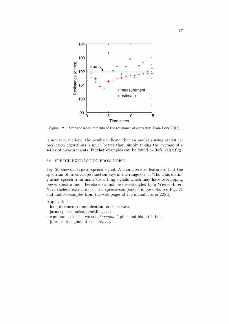
Example [Levy[21](e)]: determine the resistance of a given

– resistor: 100Ω, 2% acuracy,

– accuracy of Ohm–meter: ±1Ω.

– System: xk = xk−1, Q = 0, (A = 1),

– measurement: zk = xk + vk, R = (1Ω)2, (H = 1),

– best estimate: x0 = 100Ω, σR = P−0 = (2Ω)2 (without measurement).

Fig. 19 diplays a simulation of the measurement and its prediction of thecorrect value. Although the assumption of a Gaussian resistance–distribution

17

Figure 19. Series of measurements of the resistance of a resistor. From Levy[21](e).

is not very realistic, the results indicate that an analysis using statisticalprediction algorithms is much better than simply taking the average of aseries of measurements. Further examples can be found in Refs.[21](d,f,g).

5.6. SPEECH EXTRACTION FROM NOISE

Fig. 20 shows a typical speech signal. A characteristic feature is that thespectrum of its envelope function lays in the range 0.8 . . . 7Hz. This distin-guishes speech from many disturbing signals which may have overlappingpower spectra and, therefore, cannot be de–entangled by a Wiener–filter.Nevertheless, extraction of the speech–component is possible, see Fig. 21and audio–examples from the web-pages of the manufacturer[22](b).

Applications:– long distance communication on short wave

[atmospheric noise, crackling . . . ]– communication between a Formula 1 pilot and his pitch box,

[uproar of engine, other cars,. . . ].

18

Figure 20. A typical speech signal. Left: Time dependence, right: power spectrum[22](a).

Figure 21. Extraction of speech (right) from a noisy signal (left). From Ref.[22](b).

5.7. COCKTAIL PARTY PROBLEM

Consider a situation where there are N different signals sj(t) (within thesame bandwidth) which are recorded as linear superpositions xi(t) (yetwith unknown mixing ratios) by M different detectors. How to extractthe sj(t)? This is the field of Independent Component Analysis (ICA) alsotermed Blind Source Separation (BSS)[23](a,b).

Typical examples involving many sources and detectors are

– Cocktail–Party-Problem[23](a-c), see Fig. 22,– separation of radar signals by an array of antennas[23](d),

– analysis of seismic signals[23](e),

– separation of biomagnetic sources, like electro–encephalograms (EEG)[23](f).

A simple situation occurs for two signals s1(t) and s2(t) (i.e. two “speak-ers”). The mixture of both signals reaches two microphones (i.e. two “ears”of another person) one wants to separate both sources

xi(t) =N=2∑

j=1

Aijsj(t), i = 1 . . .M(= 2).

Humans tackle the problem using the directivity of their ears, the knowncharacter of the voice in question, and their own “built–in personal com-

19

Figure 22. The Cocktail–Party problem: What did she say??

Figure 23. Blind source separation of two signals[23](c).

puter”. In contrast to the previous problem of chapts.5.6, several signals ofthe same type must be de–entangled.5

A surprising simple and powerful method to the problem can be foundby claiming the statistical independence of the signals[23](a,c), i.e. mini-mizing the cross correlation between u1(t) and u2(t) in terms of Wij

ui(t) =N

∑

j=1

Wij xj(t).

The ui(t) represent a statistical estimate of sj(t), see Fig. 23.

5 The mixing matrix A is unknown and possibly singular.

20

Ψ(x)0

−2 210−1

0.5

1

1.5a) b)

x

V(x)

L C Q,U

I

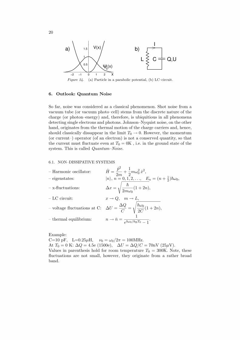
Figure 24. (a) Particle in a parabolic potential, (b) LC–circuit.

6. Outlook: Quantum Noise

So far, noise was considered as a classical phenomenon. Shot noise from avacuum tube (or vacuum photo–cell) stems from the discrete nature of thecharge (or photon–energy) and, therefore, is ubiquitious in all phenomenadetecting single electrons and photons. Johnson–Nyquist noise, on the otherhand, originates from the thermal motion of the charge carriers and, hence,should classically dissappear in the limit T0 → 0. However, the momentum(or current–) operator (of an electron) is not a conserved quantity, so thatthe current must fluctuate even at T0 = 0K , i.e. in the ground state of thesystem. This is called Quantum–Noise.

6.1. NON–DISSIPATIVE SYSTEMS

– Harmonic oscillator: H =p2

2m+

1

2mω2

0 x2,

– eigenstates: |n〉, n = 0, 1, 2, . . ., En = (n + 12)~ω0,

– x-fluctuations: ∆x =

√

~

2mω0(1 + 2n),

– LC circuit: x → Q, m → L,

– voltage fluctuations at C: ∆U =∆Q

C=

√

~ω0

2C(1 + 2n),

– thermal equilibrium: n → n =1

e~ω0/kBT0 − 1.

Example:C=10 pF, L=0.25µH, ν0 = ω0/2π = 100MHz.At T0 = 0 K: ∆Q = 4.5e (1500e), ∆U = ∆Q/C = 70nV (25µV).Values in parenthesis hold for room temperature T0 = 300K. Note, thesefluctuations are not small, however, they originate from a rather broadband.

21

Z(ω)

a)

U

I

C

LR

b)

Unoise

R

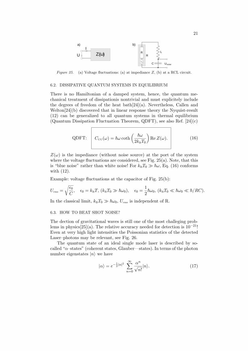
Figure 25. (a) Voltage fluctuations: (a) at impediance Z, (b) at a RCL circuit.

6.2. DISSIPATIVE QUANTUM SYSTEMS IN EQUILIBRIUM

There is no Hamiltonian of a damped system, hence, the quantum me-chanical treatment of dissipationis nontrivial and must explicitely includethe degrees of freedom of the heat bath[24](a). Nevertheless, Callen andWelton[24](b) discovered that in linear response theory the Nyquist-result(12) can be generalized to all quantum systems in thermal equilibrium(Quantum Dissipation Fluctuation Theorem, QDFT), see also Ref. [24](c)

QDFT: CUU(ω) = ~ω coth

(

~ω

2kBT0

)

Re Z(ω). (16)

Z(ω) is the impediance (without noise source) at the port of the systemwhere the voltage fluctuations are considered, see Fig. 25(a). Note, that thisis “blue noise” rather than white noise! For kBT0 À ~ω, Eq. (16) conformswith (12).

Example: voltage fluctuations at the capacitor of Fig. 25(b):

Urms =

√

ε0C

, ε0 = kBT, (kBT0 À ~ω0), ε0 =1

2~ω0, (kBT0 ¿ ~ω0 ¿ ~/RC).

In the classical limit, kBT0 À ~ω0, Urms is independent of R.

6.3. HOW TO BEAT SHOT NOISE?

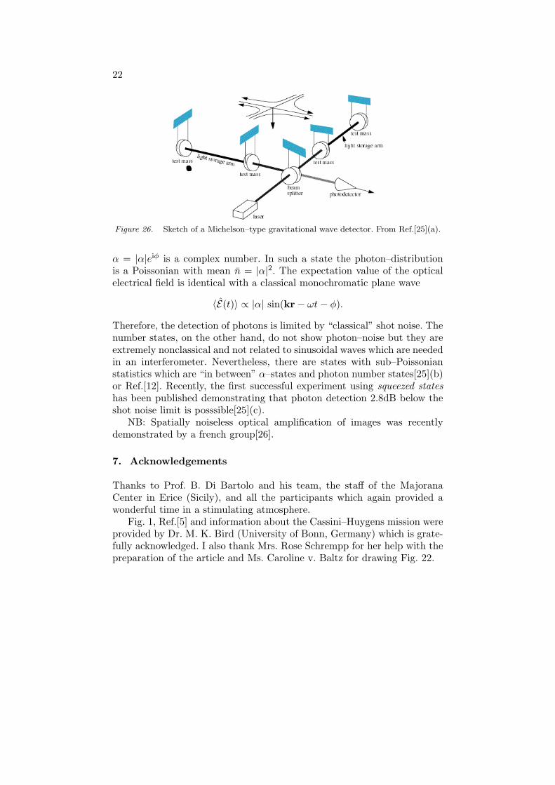
The dection of gravitational waves is still one of the most challeging prob-lems in physics[25](a). The relative accuracy needed for detection is 10−21!Even at very high light intensities the Poissonian statistics of the detectedLaser–photons may be relevant, see Fig. 26.

The quantum state of an ideal single mode laser is described by so-called “α–states” (coherent states, Glauber—states). In terms of the photonnumber eigenstates |n〉 we have

|α〉 = e−12|α|2

∞∑

n=0

αn

√n!|n〉. (17)

22

Figure 26. Sketch of a Michelson–type gravitational wave detector. From Ref.[25](a).

α = |α|eiφ is a complex number. In such a state the photon–distributionis a Poissonian with mean n = |α|2. The expectation value of the opticalelectrical field is identical with a classical monochromatic plane wave

〈E(t)〉 ∝ |α| sin(kr − ωt − φ).

Therefore, the detection of photons is limited by “classical” shot noise. Thenumber states, on the other hand, do not show photon–noise but they areextremely nonclassical and not related to sinusoidal waves which are neededin an interferometer. Nevertheless, there are states with sub–Poissonianstatistics which are “in between” α–states and photon number states[25](b)or Ref.[12]. Recently, the first successful experiment using squeezed states

has been published demonstrating that photon detection 2.8dB below theshot noise limit is posssible[25](c).

NB: Spatially noiseless optical amplification of images was recentlydemonstrated by a french group[26].

7. Acknowledgements

Thanks to Prof. B. Di Bartolo and his team, the staff of the MajoranaCenter in Erice (Sicily), and all the participants which again provided awonderful time in a stimulating atmosphere.

Fig. 1, Ref.[5] and information about the Cassini–Huygens mission wereprovided by Dr. M. K. Bird (University of Bonn, Germany) which is grate-fully acknowledged. I also thank Mrs. Rose Schrempp for her help with thepreparation of the article and Ms. Caroline v. Baltz for drawing Fig. 22.

23

8. Appendix A

The following Huygens–to–earth radio link parameters have been takenfrom Folkner et al.[4](b) to estimate the signal and noise voltages at thereceiver at the Green Bank Telescope (GBT) in West Virginia, USA. Theultrastable signal at 2.040 GHz was down–converted to 300kHz and sampledat a rate of 1.25Mhz with 8 bit resolution.

– distance Titan – Earth: d ≈ 8AU, (1AU≈ 150 × 106km),

– Huygens radiation power: P = 10.6W, (3dB beam width: 120degree),

– at GBT receiver: Pin ≈ 2.8 × 10−21W,

Uin = 3.7 × 10−10V, (at R = 50Ω),

– thermal noise: U2rms = 4 kBT0 R ∆ν, (∆ν = 1Hz, T0 = 30K),

– power–matching: Unoise= Urms/2 ≈ 1.4 × 10−10V,

Pnoise= U2noise/R = 1.6 × 10−21W.

– estimated S/N ratio: S/N ≈ 8dB.

References

1. (a) A. V. Oppenheim and A. S. Willsky, eds. (1983), Signals and Systems, PrenticeHall;(b) J. L. Lacoume et al., eds. (1987), Signal Processing, North Holland;(c) http://en.wikipedia.org/wiki/Signal processing.

2. L. A. Wainstein and V. D. Zubakov (1962), Extraction of Signals from Noise,Prentice Hall.

3. (a) http://www.gb.nrao.edu/GBT/GBT.shtml; http://www.nrao.edu/news/newsletters/;(b) http://en.wikipedia.org/wiki/Green Bank Telescope.

4. (a) M. K. Bird et al. (2006), NRAO Newsletters 107, 3, see Ref. [3](a);(b) W. M. Folkner et al. (2006), J. Geophys. Res. 111, E07S02;(c) M. K. Bird, personal communication.

5. Cassini Huygens – Huygens Probe Mission Description (Dec. 2004),Jet Propulsion Laboratory, CALTEC, JPL D-5564, Rev. O (suppl., ver. 2).

6. (a) Moon reflection signals (EME): http://www.moonbounce.info/wav.html;(b) Mars Global Surveyor Relay Test:

http://ourworld.compuserve.com/homepages/demerson/.7. (a) http://en.wikipedia.org/wiki/Fourier transform;

(b) http://en.wikipedia.org/wiki/Discrete Fourier transform.8. (a) http://www.h-wolff.de/;

(b) http://www.w1vd.com/;(c) http://www.w1tag.com/.

9. W. H. Press et al. (2003), Numerical Recipes in C, Cambridge.10. H. Babovsky et al. (1987), Math. Methoden der Systemtheorie: Fourieranalysis,

Teubner.11. Telefunken A.G. (1963), Mechanische Filter, Telefunken Zeitung Jg. 36, Heft 5, 275.

24

12. R. v. Baltz (2005), Photons and Photon Statistics: From Incandescent Light to

Lasers. In: Frontiers of Optical Spectroscopy, B. Di Bartolo and O. Forte, eds.,Springer.

13. R. Landauer (1998), Nature 392, 658.14. (a) N. G. van Kampen (1983), Stochastic Processes in Physics and Chemistry, North

Holland;(b) http://en.wikipedia.org/wiki/Statistics.

15. (a) J. L. Passmore et al. (1995), Am. J. Phys. 63, 592;(b) Y. Kraftmakher (1995), Am. J. Phys. 63, 932;(c) W.T. Vetterling and M. Andelman (1979), Am. J. Phys. 47, 382.

16. (a) W. Schottky (1918), Ann. Phys. (Leipzig), 57, 541;(b) J. B. Johnson (1925), Phys. Rev. 26, 71.

17. (a) J. B. Johnson (1928), Phys. Rev. 32, 97;(b) H. Nyquist (1928), Phys. Rev. 32, 110.

18. (a) Perkin Elmer: http://www.cpm.uncc.edu/lock in 1.htm;(b) R. Wolfson (1991), Am. J. Phys. 59, 569;(c) J. H. Scofield (1994), Am. J. Phys. 62, 129;(d) K. G. Libbrecht et al. (2003), Am. J. Phys. 71, 1208.

19. A. Th. Forrester et al. (1955), Phys. Rev. 99, 1691.20. http://en.wikipedia.org/wiki/Teleprinter.21. (a) R. E. Kalman, Trans. ASME J. Basic Eng. 82(Series D), 35 (1960);

(b) G. Welch and G. Bishop, An Introduction to the Kalman–Filter,http://www.cs.unc.edu/∼welch/kalman/index.html;

(c) P. D. Joseph, http://ourworld.compuserve.com/homepages/PDJoseph/;(d) R. Webster and G. B. M. Heuvelink (2006), Eur. J. Soil Sci. 57, 758;(e) L. J. Levy, http://www.cs.unc.edu/∼welch/kalman/Levy1997/index.html;(f) D. Simon, The Kalman Filter: Navigation’s Workhorse,

http://www.innovatia.com/software/papers/kalman.htm;(g) D. Mackenzie (2003), SIAM News 36, No. 8.

22. (a) Found somewhere on the WWW;(b) http://www.Ing-Michels.de.

23. (a) Hyvarinen, A. et al. (2001), Independent Component Analysis, Wiley;(b) http://en.wikipedia.org/wiki/Cocktail party effect;

http://en.wikipedia.org/wiki/Blind signal separation;(c) K. R. Muller: http://www.first.fraunhofer.de/ida;

http://ddi.cs.uni-potsdam.de/HyFISCH/Spitzenforschung/Mueller.htm;(d) F. Cristopher and C. Morrisean (1985), Proc. Xeme Coll. GRETSI, 1017;(e) S. Williamson et al., eds. (1990). Advances in Biomagnetism, Plenum;(f) F. Acernese et al. (2003), IEEE Trans. Neur. Netwks. 14, 167.

24. (a) T. Dittrich et al., eds. (1998), Quantum Transport and Dissipation, Wiley-VCH;(b) H. B. Callen and T. A. Welton (1951), Phys. Rev. 83, 34;(c) L. Banyai (1985), Z. Phys. B 58, 161.

25. (a) http://en.wikipedia.org/wiki/Gravitational wave;(b) R. E. Slusher and B. Yurke (1988), Unterdruckung des Quantenrauschens bei

Lichtwellen, Spektrum der Wiss., Juli–Heft, S. 70, (Sci. Am., June 1988?);(c) H. Vahlbruch et al. (2005), Phys. Rev. Lett. 95, 211102.

26. A. Mosset et al. (2005), Phys. Rev. Lett. 94, 223603.