External coupling between CFD and energy simulation :implementation and validationCitation for published version (APA):Djunaedy, E., Hensen, J. L. M., & Loomans, M. G. L. C. (2005). External coupling between CFD and energysimulation : implementation and validation. ASHRAE Transactions, 111(1), 612-624.

Document status and date:Published: 01/01/2005

Document Version:Accepted manuscript including changes made at the peer-review stage

Please check the document version of this publication:

• A submitted manuscript is the version of the article upon submission and before peer-review. There can beimportant differences between the submitted version and the official published version of record. Peopleinterested in the research are advised to contact the author for the final version of the publication, or visit theDOI to the publisher's website.• The final author version and the galley proof are versions of the publication after peer review.• The final published version features the final layout of the paper including the volume, issue and pagenumbers.Link to publication

General rightsCopyright and moral rights for the publications made accessible in the public portal are retained by the authors and/or other copyright ownersand it is a condition of accessing publications that users recognise and abide by the legal requirements associated with these rights.

• Users may download and print one copy of any publication from the public portal for the purpose of private study or research. • You may not further distribute the material or use it for any profit-making activity or commercial gain • You may freely distribute the URL identifying the publication in the public portal.

If the publication is distributed under the terms of Article 25fa of the Dutch Copyright Act, indicated by the “Taverne” license above, pleasefollow below link for the End User Agreement:www.tue.nl/taverne

Take down policyIf you believe that this document breaches copyright please contact us at:openaccess@tue.nlproviding details and we will investigate your claim.

Download date: 24. Mar. 2020

EXTERNAL COUPLING BETWEEN CFD AND ENERGY SIMULATION: IMPLEMENTATION AND VALIDATION

Keywords: building energy simulation, computational fluid dynamics, coupled simulation, external coupling, validation Authors: E. Djunaedy J.L.M. Hensen, PhD M.G.L.C. Loomans, PhD E. Djunaedy is PhD candidate and J.L.M. Hensen is professor in the Department of Architecture, Building and Planning, Technische Universiteit Eindhoven, Netherlands. M. G. L. C. Loomans is scientific researcher at The Netherlands Organisation for Applied Scientific Research (TNO).

EXTERNAL COUPLING BETWEEN CFD AND ENERGY SIMULATION: IMPLEMENTATION AND VALIDATION

ABSTRACT

This paper describes the implementation of external coupling between building energy simulation and CFD. Internal coupling is the “traditional” way of developing software, i.e. expanding the capabilities of existing software by adding new modules into an existing package. External coupling on the other hand makes use of existing packages in different domain (for example the thermal domain for energy simulation and the flow domain for CFD), and provides a mechanism for these packages to communicate.

A summary of the latest development is persented to put external coupling into the context. The implementation of external coupling is then summarized. The paper concludes with a case study to validate the performance of external coupling, and to highlight its potentials.

INTRODUCTION

The coupling of building energy simulatioon (BES) and computational fluid dynamics (CFD) simulation has been discussed in various publication in recent years, e.g. Negrao (1998), Srebric et al (2000), Beausoleil-Morrison (2002), Zhai et al (2002). The two simulation programs, as in any simulation program, have their own limitations. For example, the boundary conditions of CFD are usually assumed with limited consideration for the thermal storage effects of the wall, external conditions and interactions with building services systems. BES calculates its energy prediction based on a well-mixed assumption so that the definition of the convective heat transfer coefficient (CHTC) cannot capture the dynamics of the flow near the surfaces.

The coupling (or “integration”) between the two programs is seen as an alternative to achieve better results because the two can provide boundary conditions to each other. For example, BES can provide internal surface temperatures of the walls to CFD, while CFD can provide more accurate CHTC for BES. The benefits of the coupled simulation has been discussed in the publications mentioned.

Djunaedy et. al (2003) discussed different approaches to couple the two programs. Here, internal coupling is regarded the “traditional” way of coupling, i.e. expanding the capabilities of existing software by adding new modules into an existing program. Internal coupling can also be seen as subroutinazation. External coupling on the other hand makes use of existing packages in different domain (for example the thermal domain for energy simulation and the flow domain for CFD), and provides a mechanis m for these programs to communicate.

This paper describes the implementation of external coupling between BES and CFD. In the first sections external coupling is put into the context by summarizing the latest development in this area. Next, a case study is presented to justify the use of the external coupling approach, and to highlight its potentials.

EXTERNAL COUPLING

External coupling could mean exchanging data between two programs sequentially, where a model-preprocessor transforms the output of one prog ram into an input for another program after the first program completed the simulation. For this study, “external coupling” is defined as run-time communication between two separate program where at least one of the program continues to run while exchangin g information with the other program.

There are at least two reasons to use external coupling. Firstly, each domain application has evolved separately over the years and is well proven. Rewriting the code (to be included as part of a package in another domain) could be seen as a set back from these independent advances in separate domains. Therefore, further efforts should better be concentrated at making these different domain applications to communicate with each other.

Secondly, external coupling can immediately benefit from independent developments in each domain. The separate domain applications can expand and develop in their respective directions, and the external

coupling mechanism can make this development available without having to (heavily) update the source code.

DIFFERENT IMPLEMENTATIONS OF COUPLING STRATEGIES

The focus point of coupling between CFD and BES can be represented by the convection heat transfer equation on the internal surfaces:

)( refwallc TThAq −=

where: qc : convective heat flux (W)

h : conventive heat transfer coefficient (CHTC) (W/m2K)

A : wall surface area (m2)

Twall : wall temperature (°C)

Tref : reference temperature (°C)

The energy calculation of the BES is sensitive to the value of the CHTC and the reference temperature used in the above equation. Without CFD, the best BES can do is to adaptively use empirical correlations during the simulation, and use the air-point temperature as reference temperature. The main disadvantage is that it cannot include the effect of temperature stratification around the wall, and also the difference in flow characteristics between surfaces in the same room. CFD is introduced to overcome those problems. However, the parameters in the equation must be resolved iteratively, by exchanging the parameters between the two programs until the values are converged.

Negrao (1995) describes two handshaking mechanisms between the BES and CFD: the surface coupling and integrated coupling. Negrao uses the word “conflation” for coupling. However for consistency, coupling will be used in this paper.

In integrated coupling, CFD interacts directly with the thermal matrix solver and resolves the exchanged parameters until the values are converged. CFD is used to solve the zone air-point temperature and the internal surface convection, while the BES provides the CFD with the internal surface temperatures. Both iteratively exchange the data until convergence before moving to the next time step.

In surface coupling, on the other hand, the two programs work independently and exchange information at the internal surfaces. The CFD uses the boundary conditions (wall temperature) from the previous time step, calculates the convection heat transfer coefficient (CHTC) and sends this back to the BES. The BES will then use this information to form the matrix for the zone heat balance equations and solves the matrix for the current time step. The simulation continues with CFD simulations always use the data from the previous time step.

Beausolleil-Morrison (2000) argued that surface coupling brings many advantages over the integrated approach. For external coupling, the most important feature is that the surface coupling provides more flexibility in defining the coupling mechanism. With regard to accuracy, obviously integrated coupling is more accurate because it resolves the exchanged data in many iterations until converged to a certain value. Beausolleil-Morrison (2000) also argued that the accuracy will be the same if the time step is sufficiently small, although he did not elaborate on how small is small.

Chen and Zhai (2001) found that in the iteration between CFD and BES, the solution does exist and is unique. Chen and Zhai also reported that normally convergence can be reached after 4 – 10 iterations. If we take one hour as the standard time step in most BES, we can conclude that a 6 to 15 minutes time step is small enough for surface coupling to get the same accuracy as the integrated coupling.

Furthermore, the CFD-predicted value of CHTC (CHTCCFD) can always be rejected in surface coupling. This cannot be done in integrated coupling without interrupting the iteration process. This checking mechanism of the CHTCCFD value before passing it back to BES is one of the quality assurance measures that should be used when using surface coupling.

COUPLING MECHANISM

Figure 1 gives an overview of the current status of surface coupling (Beausolleil-Morrison 2000 and ESRU 2000) . In summary, for every time step during the calculation of the convection heat transfer coefficient (CHTC) of internal surfaces, the thermal domain checks whether there is any CFD call defined for that time step. If not, it continues with another mechanism for defining the CHTC of the internal surfaces. If yes, it will invoke the coupling controller to derive the CHTC from a CFD simulation. The coupling mechanism consists of a pre-CFD treatment, (final) the actual CFD simulation and a post-CFD treatment.

The pre-CFD treatment involves an investigative CFD simulation (so actually there are two CFD simulations for every CFD call). This investigative CFD simulation (the so-called “gopher run”) is a simple CFD simulation (with coarse mesh and simple turbulence model) that will classify the flow regime near each surface. Based on this classification, the coupling controller decides which boundary conditions are applied for the final CFD simulation.

The final CFD simulation mainly uses the standard k-ε turbulence model. However, apart from sending the wall temperature to CFD, the coupling controller decides (1) which wall function to use, (2) whether the CHTC derived from an empirical correlation should also be sent to CFD and (3) what reference temperature should be used in CHTC calculation in CFD. After the final CFD simulation, the post-CFD treatment will calculate the CHTC for each internal surface based on the CFD result, i.e. the CHTCCFD , and decides whether the predicted CHTC can be used for further calculation in thermal domain.

Note that the CHTCCFD is not calculated solely by CFD. Beausoleil-Morrison (2001) noted that the use of the CFD definition of CHTC is the most desired approach. However, its own limitation to accurately predict the surface heat convection makes it not a fully viable approach. For that reason Beausoleil-Morrison argued that the “co-operative” approach is the solution, as long as the CFD solution is regarded not accurate enough to get reasonably accurate results on its own in all flow configurations.

Figure 1.. Internal coupling mechanism in BES

In the co-operative approach, CFD will calculate the convective heat transfer on the wall based on the

boundary conditions set by the coupling controller. Depending on the type of boundary conditions set, there are 8 different ways of calculating the convective heat transfer on the wall (the details can be found in Beausolleil-Morrison, 2000). The calculated convective heat transfer is passed back to BES where it will be converted to CHTCCFD using the BES air-point temperture as the reference temperature. There is an inconsistency in using the reference temperature between the CFD and BES: the CFD uses local temperature (i.e. the air temperature in the adjacent cells) while BES uses the air-point temperature. This inconsistency has been acknowledged by Beausolleil-Morrison (2000). However, the co-operative apprach seems to be able to predict the impact of stratification on the wall.

The calculated CHTCCFD is then compared with a CHTC value that is determined from empirical correlations applicable to the flow field under investigation. If CHTCCFD falls within a certain predefined range, then it will be accepted and passed to the thermal domain. If not, it will be rejected and the thermal domain continues the calculation using the CHTC derived from the empirical correlation.

The initial implementation of the external coupling uses an external CFD program for the final CFD simulation, while keeping the rest of the mechanism unmodified. This assumes that the BES has the internal capability to do the investigative CFD simulation. The result of the external CFD program will be passed back to the BES (or more specifically the CFD module of the BES) in terms of field values. This further assumes that the CFD module of the BES should also have exactly the same mesh to avoid interpolation of CFD results.

As a starting point, an advanced building energy program that meets the above requirements was selected (ESRU 2000). A commercial CFD package was also selected (Fluent, 2003). However, the results of this study would apply for any BES and CFD program, with the described criteria.

However, as will be shown later, this initial implementation has several drawbacks. The pre-CFD treatment was designed to send boundary conditions (for the final CFD simulation) based on the standard k-ε turbulence model. This model is known to be less accurate for a coarse mesh, and in particular it is dependent on the size of the first grid cell adjacent to the wall (Yuan 1995). The obvious solutions for this are to refine the mesh, up to the point of practicality, or simply use another turbulence model.

The use of another (simpler) turbulence model at this point is more attractive, as refining the mesh is less practical. This is due to the limitation of the available internal CFD program, where the coupling controller can only read one mesh for both the investigative and the final CFD simulation. If the mesh for the CFD simulation would be refined, then the computation time will increase significantly as the investigative CFD run will also use the same mesh.

The zero equation turbulence model (Chen and Xu 1998) is regarded applicable for the above purpose because:

1. it uses less computing resource than the standard k-ε turbulence model.

2. it does not make use of wall functions.

3. the CHTC can be explicitly defined using the Reynolds analogy:

x

ch p

eff

eff

∆=

Pr

µ

where: h : conventive heat transfer coefficient (CHTC) (W/m2K)

µeff : effective viscosity (Pa s)

Preff : effective Prandtl number (=0.9)

cp : specific heat (J/kg K)

∆x : distance between the surface to the adjacent cell (m)

4. it has been successfully used for the coupling of CFD and energy simulation (Chen et al 1999). As the final CFD simulation does not use the standard k-ε turbulence model, then there is no reason to

do the investigative CFD run. It should be noted that the investigative CFD simulation is still an advanced

coupling mechanism. However, its implementation so far is limited to the standard k-ε turbulence model. Since the zero equation turbulence model will be used for the (final) CFD simulation, the investigative CFD simulation becomes irrelevant. Further works on this is on-going and will be reported in the near future.

The following mechanism reflects the latest developments on external coupling between CFD and BES: 1. During the calculation of the CHTC for the internal surfaces BES checks if a CFD simulation is

specified for the current time step. If not, it will continue to calculate the CHTC based on user input.

2. If yes, the BES will invoke the coupling controller which will call the external CFD program to run the CFD simulation (using the zero equation turbulence model).

3. After the simulation, the CFD program calculates the CHTC for each internal surface and sends the result back to the coupling controller.

4. If the CHTC falls within pre-defined criteria, the coupling controller will pass the result to the BES, otherwise the coupling controller will send a flag to BES to use its own CHTC value. The following assumptions/limitation applies to the current implementation:

1. Radiative heat exchange is not included in the CFD simulation. As the BES includes the radiation in its calculation, this will affect the boundary conditions sent to CFD, wh ich in turn will make CFD to over-predict the CHTC value. How significant is the effect of this omission is recognized as an important future work for this study.

2. The external coupling implementation uses the surface coupling mechanism, even though the integrated conflation is obviously more accurate. The reasons are, firstly, because it could have the same accuracy if the time step is small. Secondly, because of the data exchange mechanism employed by the current implementation is using the intermediate fi le, which is not fast enough for integrated coupling. Another data exchange mechanism is the inter-process communication (IPC) which is the subject of an on-going research (Yahiaoui et. al. 2004). Integrated coupling mechanism can be easily implemented for external coupling once there is a faster mechanism for data exchange.

3. The CFD calculations are steady state for every time step of BES simulation. However, on higher level view, all of the CFD simulations are more like quasi-steady simulations that change its boundary conditions every (BES) time step. The use of transient CFD simulation is intentionally avoided as it is more computationally expensive, and in this case this is justified by the fact that:

• the simulation is stable and can reach the convergence without difficulty. • there is no transient parameter (within BES time step) needed for the result.

4. The current implementation depends on the capability of BES to provide an extensive range of empirical correlation of CHTC, against which the CHTC prediction from CFD is checked. If there is no such library available, then the only way to use external coupling is to manually specify a range of acceptable values of CHTC. This range would have to be hard-coded into the source code, and this will make the mechanism less flexible as this range could be different for a different problem.

CASE STUDY

The above discussion on internal and external coupling is supported by a case study in which the separate coupling mechanisms are compared. The case study is derived from Lomas et al (1994) and is described in the remaining of this paper.

Figure 2. Test cell site (Photo from Lomas et al 1994)

BES model

The test cell under investigation is located in Bedfordshire, UK. Figure 2 shows the site layout and the situated test cells . The site has eight semi-detached rooms, which have a lightweight, timber framed, construction. These rooms have interchangeble glazing panels in the south walls, and the one used for the current study has a double glazed panel.A detailed descrip tion of the site and the test room can be found in Lomas et al (1994).

Figure 3 shows the BES model that has been used for this study. The geometry and construction is built according to the report without modification, including the small construction in the edges of the test cells.

The following assumptions were used when creating the model: • The test cells were developed in pairs. However, the wall connecting the neighbouring cell is heavily insulated. For this reason, only one of the cells is modelled. • The cell on the other side however is explicitly modelled as it obstructs solar radiation. The BES program uses the sun-tracking algorithm to calculate the solar shading. • The geometric view factors were calculated using a ray-tracing procedure. • The default sky model (the Perez anisotropic model) was used to estimate the amount of diffuse solar radiation striking the building surfaces. • The default insolation algorithm, as used by the BES, was used to calculate the distribution of solar beam radiation to the room’s internal surfaces. • The fabric thermal property data provided in the IEA report were used unmodified. • No humidity data were provided in the IEA study for the October heating period, so typical values for England were assumed. • Convection coefficients for external surfaces were calculated using the default correlation (i.e. Alamdari-Hammond correlation).

Figure 3. BES model

CFD model

Beausolleil-Morrison (2000) in an earlier study used a simplified model for the CFD-coupled simulation (internal). The simplified model did not include the small construction in the corner of the test cell. This simplification was needed because of computer restrictions. Including small construction would need a finer mesh to model, which would result in a longer computation time. With the simplification, the mesh size was 6x9x9.

Because of the difference in the model, the CFD-coupled simulation could not be compared with the uncoupled simulation. Furthermore, the study concluded that the prediction of the convective heat transfer coefficient (CHTC) was not good with the mesh size of 6x9x9. It was suggested that better result would be achieved with a finer mesh.

For that reason, no simplification was attempted for this study. The grid size of 0.1m was required to capture the small construction. This resulted in a mesh size of 5x23x23.

Simulations setting

There are 2 sets of measurement data, each contains 10 days of experiment (however, the first 3 days are considered as a start-up period to minimize the effect of the initial conditions). One set of data is for heating condition (in October) and the other one is for free-floating condition (in May).

For this study, only the heating situation was considered. The recorded outdoor conditions are (average values): external temperature of 8.8 °C, global and diffuse horizontal solar radiation of 77 and 32 W/m2 respectively, and wind speed of 1.6 m/s. The range of daily maximum values for global and diffuse solar radiation are 49 – 412 W/m2 and 47 – 211 W/m2.There is no record of relative humidity, so for simulation a typical value for England is used. All climate data (except for relative humidity) used in the simulation were the actual measured data.

Table 1 shows a summary of the simulation settings. Cases 1 to 3 were carried out to establish confidence in the coupling mechanism shown in Figure 1. Based on the result of these 3 cases, some modifications were introduced, and the last two cases were simulated using the modified mechanism.

Table 1 Summary of simulation setting

CHTC definition on internal surfaces

Gopher run Turbulence model (final CFD run)

Case 1 (base case) Alamdari-Hammond (1983) correlation

n.a. n.a.

Case 2 Heater off: • Alamdari -Hammond

(1983) correlation Heater on:

• Wall: Khalifa and Marshal (1990) correlation

• Floor: Alamdari-Hammond (1983) correlation

n.a. n.a.

Case 3 Internal coupling yes Standard k-e Case 4 Internal coupling no Indoor Zero Equation Case 5 External coupling no Indoor Zero Equation

The room was heated during the day from 06:00 to 18:00. The heater was modelled as a heat source with the same maximum heat output as in the experiment. The heat output was divided, as estimated in the report (Lomas et al 1994), in a ratio 40:60 for convection and radiation. In the experiment, a PID controller was used for the heater. The simulation uses an ideal controller to inject the heat into the room.

The test rooms were tightly sealed and the experiment was conducted with zero air infiltration assumption. This was also assumed for the simulation.

The simulation time step is 15 minutes. For CFD-coupled simulations, CFD was invoked only on the last day when the heater was on (i.e. from 06:00 to 18:00 on 26-Oct). The CFD simulations, both for internal coupling and external coupling, used the same convergence criteria (i.e. 10-6 residuals error for energy and 10-3 for others). The iteration for CFD simulations were limited to 500 iterations, and the iteration always starts from the latest data from the previous timestep.

INITIAL RESULTS: SETTING UP THE BASE CAS E

In this section, the results of Case 1 – 3 are presented. This has two objectives. Firstly, to ensure that all parts of the experiment are modelled correctly. This is done by comparing the result of this study with earlier results by Lomas et al (1994). Secondly, to evaluate the current capabilities of internal coupling.

Figure 4 shows the room temperature fluctuations for 7 days. The predicted temperature can follow the fluctuations. The temperature decay is particularly accurate with the maximum error of less than 2 °C occurred when the temperature started to rise again. The simulation predicted a faster rate of temperature rise due to the assumption of ideal controller used in the simulation.

However, there are big differences for a few hours in the afternoon from day 2 to day 5. During this period, the simulated room temperature has a similar pattern, regardless the pattern of the measurement result. The following are the possible causes for this discrepancy in the room temperature:

• These are the time steps where the solar radiation was very high. The BES result is known to be sensitive to the definition of the sky model. The current problem could be caused by the default sky model (the Perez anisotropic model), that was used to estimate the amount of diffuse solar radiation striking the building surfaces, and its insolation algorithm (that was used to calculate the distribution of solar beam radiation to the room’s internal surfaces).

• The measurement error which was estimated around 20% (of absolute temp erature). Furthermore, the measurement points were not specified. The air temperature was recorded at three heights

(low, middle, high) without any further details on the exact location. The air temperature data presented in this paper is from the middle point.

To avoid the above problem further detailed discussion has been focussed on the days where solar radiation is not high, i.e. the last day of the experiment (26-Oct). As can be seen in Figure 5, the temperature prediction is very close. The difference occurred when the heater is on (at 06.00) and when the heater is off (18:00). The temperature reached the steady state value within 2 or 3 hours in the simulation, while in the experiment it took 5 hours. This is solely attributed to the ideal controller that is used in the simulation, as opposed to much slower PID controller as used in the experiment.

Figure 6 shows the energy consumption for the whole period of simulation. The base case result (67.9 MJ) is similar to the previous result that was derived with an earlier version of BES as reported in Lomas et al (1994). This gives confidence in the current model.

Applying an empirical specification of CHTC results in a higher energy consumption, increasing around 5%. This is attributed to the higher CHTC during the time when the heater is on, around 10 W/m2K compared to around 3 W/m2K for the base case (Figure 7).

The effect of applying a CFD-coupled simulation is significant in terms of energy consumption prediction. Figure 8 shows the energy consumption for one day (as coupled simulation is carried out only for this day). Using empirical CHTC increases the energy prediction by 8% compared to the base case, while using internal coupling results in a 15% increase.

However, this significant increase in the energy consumption prediction is caused by a very high CHTC (up to 80 W/m2K, as shown in Figure 9) which is not realistic for this type of flow.

The internal coupling case (Case 3) was carried out using the existing mechanism available in BES. The CHTC for the internal surfaces were calculated initially by empirical correlations (as in Case 2). During the times where the CFD is invoked, the CHTC can be updated via the CFD result. For Case 3 the applied criteria for that was:

0.1 CHTCempirical < CHTCCFD < 10 CHTCe mpirical

to accept or reject the CFD prediction of CHTC. The empirical CHTC was around 15 W/m2K for this investigated flow field. The loose criteria therefore would accept any value between 1.5 to 150 W/m2K. If the CHTCCFD was rejected, the thermal domain calculation applied the empirical value.

Figure 4. Room temperature (20-Oct to 26-Oct)

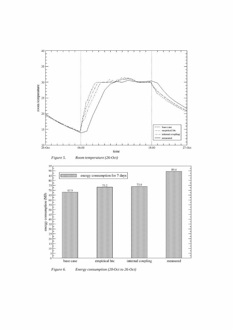
Figure 5. Room temperature (26-Oct)

Figure 6. Energy consumption (20-Oct to 26-Oct)

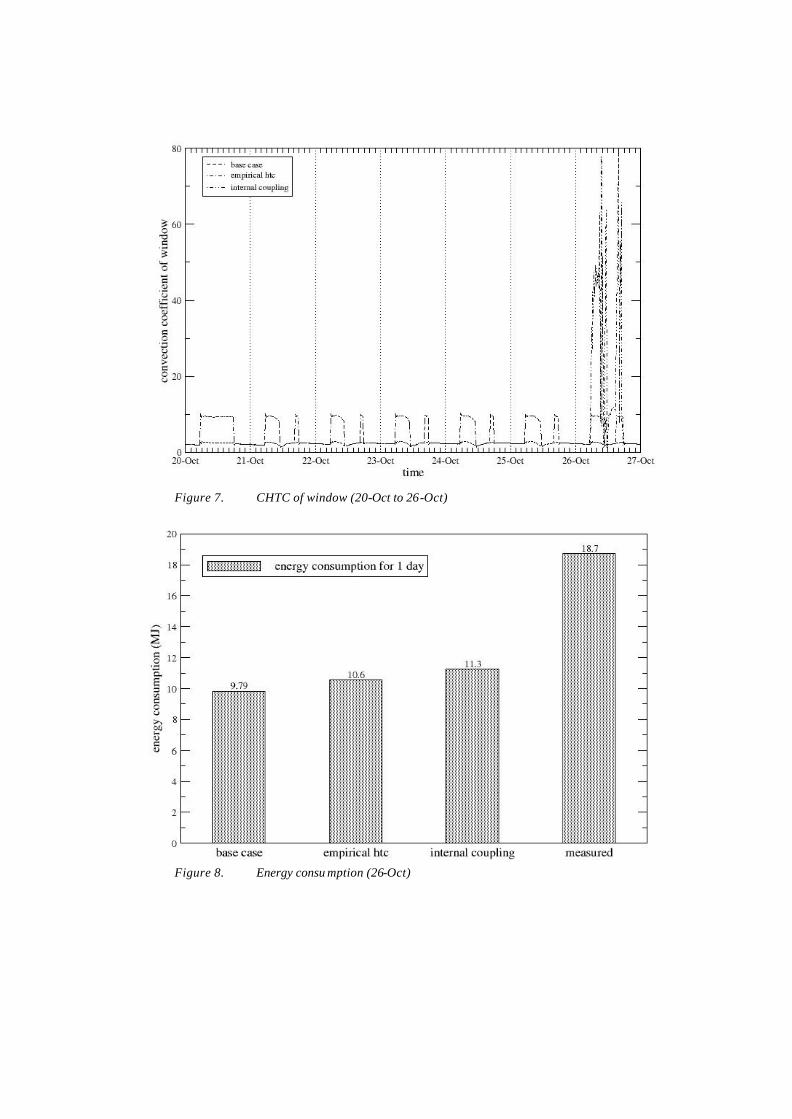
Figure 7. CHTC of window (20-Oct to 26-Oct)

Figure 8. Energy consu mption (26-Oct)

Figure 9. CHTC of window (26-Oct)

The (full) CFD simulation uses different simulation settings (turbulence model, wall function, etc) as determined by the investigative CFD simulation. For Case 3 however, standard k-ε with log-law was always selected by the coupling mechanism. Beausolleil-Morrison (2000) found that most of CHTCCFD were rejected because they were too high compared to the empirical values. He assumed that the high value was caused by the use of the standard k-ε turbulence model in combination with the log-law on a very coarse grid, so that the conditions for application of the log-law could not be met.

In this study a finer mesh (15x23x23 compared to 6x9x9) was applied. However, it still was concluded that the CHTCCFD prediction was too high. The values were accepted by the thermal domain simply because of the loose criteria. With stricter criteria (as proposed by Beausolleil-Morrison, 2000), i.e.:

0.2 CHTCempirical < CHTCCFD < 5 CHTCempirical

the values would have been rejected. The grid size adjacent to the wall is regarded as the cause for the poor performance of the turbulence model. Yuan (1995) found that the turbulence model is sensitive to the size of the first cell adjacent to the wall. In this study a uniform grid size of 100mm was applied, while Yuan (1995) found that accurate results would require a much smaller size of the first grid cell (in the order of 5mm).

The conclusion from this section is that the 15x23x23 mesh is still too coarse for standard k-ε with log-law to resolve reasonable values of CHTCCFD. Using a finer mesh is not an option as it will lead to more computation time. The other option is to use another turbulence model that can produce a reasonably good result with a coarse mesh.

Furthermore, the 15x23x23 mesh is too fine for the investigative CFD simulation. Beausolleil-Morrison (2000) reported that the investigative CFD simulation uses only a small fraction (5%) of the computing time. However, that study used a very coarse mesh (6x9x9), so the overall computing time is not high. Case 3 took 27h51m to finish with a mesh size of 15x23x23. The same case simulated using a coarser mesh (6x9x9) took only 1h14m to finish. If the investigative CFD simulation is by-passed, the simulation time can be reduced significantly.

VALIDATION OF EXTERNAL COUPLING

The cases

In this section the results of Cases 1, 2, 4 and 5 will be compared. The CFD-coupled simulations follow the changes as described in the previous section. Internal coupling, however, still uses the co-operative definition of CHTC, i.e. the definition of CHTC does not use the Reynolds analogy. External coupling, on the other hand, will use the Reynolds analogy for the definition of CHTC and passes only the CHTC values to the thermal domain.

Room air temperature

Figure 10 shows the room temperature for 1 day. The result is similar with Figure 4. Even though the rise time of the simulation is relatively faster then the experimental result, there is a noticeable difference between the 4 simulation cases. The base case rises the fastest, while the others tend to lag behind, in the order of the CHTC values. The higher the CHTC values in general, the slower the air-point temperature rises. External coupling shows the slowest response. However, it is still much too fast compared to the experiment due to the difference in the heater controller setting.

CHTC

Figure 11 shows the CHTC for the window. Most of the time, the internal coupling (Case 4) result shows exactly the same values with the empirical values (Case 2). This means that the prediction of CHTC from CFD is larger than 5 times the empirical value so that it was rejected. In that case the thermal domain used the empirical value instead of CFD-predicted value. How high the CFD-predicted values reach can be seen in the values around 06:00hrs, where they fall within the acceptance criteria. Nevertheless, they are still too high (more than 40 W/m2K) for this type of flow. The external coupling simulation (Case 5), on the other hand shows, consistently similar values for the CHTC (around 10 – 14 W/m2K), which is higher then the values calculated by empirical correlations.

For a few hours after mid-day, the empirical correlation gives the same values as the base case. The reason is that during this time, the heater controller switched the heater off, so the empirical correlation used the same correlation as the base case. The external coupling managed to follow this trend for a few time steps, but failed in some other time steps. The reason for this is that the external CFD program did not know the operation status of the heater, and simply assumes that the heater is on every time it is invoked.

Energy consumption

Figure 12 shows the energy consumption for one day. The use of empirical correlations as well as the CFD-coupled simulations give an increased prediction of energy consumption between 8% to 10%. However, it is still far too low compared to the measured value even if the error band is considered (18.7 ± 3.74).

Computing time

Table 2 shows the computing time for the performed CFD-coupled simulations. Considering the prediction of CHTC and comparing with the time required to achieve the result, external coupling shows a clear advantage over the internal coupling.

Table 2.

Comparison of computing time for CFD-coupled simulation Case Summary Time

(hr:min:sec) Case 3 Internal coupling with gopher run 27:51:46.6 Case 4 Internal coupling without gopher run 10:32:57.2 Case 5 External coupling without gopher run 00:23:56.0

Figure 10. Room temperature (26-Oct)

Figure 11. CHTC of window (26-Oct)

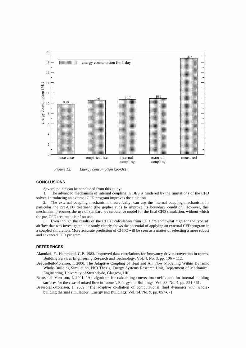
Figure 12. Energy consumption (26-Oct)

CONCLUSIONS

Several points can be concluded from this study: 1. The advanced mechanism of internal coupling in BES is hindered by the limitations of the CFD

solver. Introducing an external CFD program improves the situation. 2. The external coupling mechanism, theoretically, can use the internal coupling mechanism, in

particular the pre-CFD treatment (the gopher run) to improve its boundary condition. However, this mechanism presumes the use of standard k-ε turbulence model for the final CFD simulation, without which the pre-CFD treatment is of no use.

3. Even though the results of the CHTC calculation from CFD are somewhat high for the type of airflow that was investigated, this study clearly shows the potential of applying an external CFD program in a coupled simulation. More accurate prediction of CHTC will be seen as a matter of selecting a more robust and advanced CFD program.

REFERENCES

Alamdari, F., Hammond, G.P. 1983. Improved data correlations for buoyancy-driven convection in rooms, Building Services Engineering Research and Technology, Vol. 4, No. 3, pp. 106 – 112.

Beausolleil-Morrison, I. 2000. The Adaptive Coupling of Heat and Air Flow Modelling Within Dynamic Whole-Building Simulation, PhD Thesis, Energy Systems Research Unit, Department of Mechanical Engineering, University of Strathclyde, Glasgow, UK.

Beausoleil -Morrison, I. 2001. "An algorithm for calculating convection coefficients for internal building surfaces for the case of mixed flow in rooms", Energy and Buildings, Vol. 33, No. 4, pp. 351-361.

Beausoleil -Morrison, I. 2002. "The adaptive conflation of computational fluid dynamics with whole-building thermal simulation", Energy and Buildings, Vol. 34, No. 9, pp. 857-871.

Chen, Q., Xu W., 1998. A zero-equation turbulence model for indoor airflow simulation, Energy and Buildings, Vol. 28, No. 2, pp. 137-144

Chen, Q., Glicksman, L. R., Srebric, J. 1999. Simplified Methodology to Factor Room Air Movement and the Impact on Thermal Comfort into Design of Radiative, Convective and Hybrid Heating and Cooling Systems, ASHRAE, American Society of Heating Refrigerating and Air Conditioning, Atlanta, GA, RP-927.

Djunaedy, E., Hensen, J. L. M., Loomans, M. G. L. C. 2003. "Toward External Coupling of Building Energy and Airflow Modeling Programs", ASHRAE Transactions, Vol. 109, No. 2, pp. 771-787.

ESRU. 2000. The ESP-r system for building energy simulation, User guide for ESP-r version 9, Energy Systems Research Unit, University of Strathclyde, UK.

Fluent. 2003. Fluent user’s guide, Version 6.1, Fluent Inc., NH, USA. Khalifa A.J.N., Marshall R.H. 1990. Validation of Heat Transfer Coefficients on Interior Building Surfaces

Using a Real-Sized Indoor Test Cell, International Journal of Heat and Mass Transfer, Vol. 33, No. 10, pp. 2219 – 2236.

Lomas K J, Eppel H, Martin C, Bloomfield D. 1994. Empirical validation of thermal building simulation programs using test room data, Volume 2: Empirical validation package, UK, Watford, Building Research Establishment (BRE Ltd), c100 + diskette pp.

Negrao, C. O. R. 1995. Conflation of Computational Fluid Dynamics and Building Thermal Simulation, PhD Thesis, Energy Systems Research Unit, Department of Mechanical Engineering, University of Strathclyde, Glasgow, UK.

Negrao, C. O. R. 1998. "Integration of computational fluid dynamics with building thermal and mass flow simulation", Energy and Buildings, Vol. 27, No. 2, pp. 155-165.

Srebric, J., Chen, Q., Glicksman, L. R. 2000. "A coupled airflow and energy simulation program for indoor thermal environmental studies", ASHRAE Transactions, Vol. 106, pp. 465-476.

Yahiaoui, A., Hensen, J.L.M.., Soethout, L.L. 2004. Developing CORBA-based distributed control and building performance environments by run-time coupling, Proceedings of the 10th International Conference on Computing in Civil and Building Engineering, Weimar, Germany, pp. 86.

Yuan, X. 1995. Wall functions for numerical simulation of natural convection along vertical surfaces, PhD Thesis, Swiss Federal Institute of Technology, Zurich, Switzerland.

Zhai, Z., Chen, Q., Haves, P., Klems, J. H. 2002. "On approaches to couple energy simulation and computational fluid dynamics programs", Building and Environment, Vol. 37, No. 8 -9, pp. 857-864.