Extensible hardware for control of superconducting qubits · 2017-06-21 · Chapter 2 Theory 2.1...

U N I V E R S I T Y O F C O P E N H A G E NF A C U L T Y O F S C I E N C E

Extensible hardware for control ofsuperconducting qubits

Bachelor ThesisWritten by Daniel RamyarJune 11, 2017

Supervised byKarl David Petersson

U N I V E R S I T Y O F C O P E N H A G E NF A C U L T Y O F S C I E N C E

Faculty: Faculty of Science

Institute: The Niels Bohr Institute

Department: Center for Quantum Devices

Author: Daniel Ramyar

Email: [email protected]

Title: Extensible hardware for control of superconductingqubits

Supervisor: Karl David Petersson

Handed in: June 14, 2017

Defended: ??

Name

Signature

Date

Contents

1 Introduction 1

2 Theory 22.1 Qubits . . . . . . . . . . . . . . . . . . . . . . . . . . . . . . . . . 2

2.1.1 The Hydrogen Atom . . . . . . . . . . . . . . . . . . . . . 32.1.2 Superconducting Qubits . . . . . . . . . . . . . . . . . . . 4

2.2 The Cooper Pair Box . . . . . . . . . . . . . . . . . . . . . . . . . 72.3 Circuit QED . . . . . . . . . . . . . . . . . . . . . . . . . . . . . 92.4 Jaynes-Cummings Hamiltonian . . . . . . . . . . . . . . . . . . . 102.5 Dispersive Regime: Qubit Readout . . . . . . . . . . . . . . . . . 102.6 Gate tunable Qubits . . . . . . . . . . . . . . . . . . . . . . . . . 112.7 Single Qubit Rotations . . . . . . . . . . . . . . . . . . . . . . . . 112.8 Single Sideband Modulation . . . . . . . . . . . . . . . . . . . . . 12

3 Setup 133.1 Proposed Setup for Qubit Control . . . . . . . . . . . . . . . . . 133.2 IQ Mixer Optimization Algorithm . . . . . . . . . . . . . . . . . 14

4 Experiment 164.1 Spectroscopy . . . . . . . . . . . . . . . . . . . . . . . . . . . . . 164.2 Rabi . . . . . . . . . . . . . . . . . . . . . . . . . . . . . . . . . . 164.3 Gate tuneup / ALLXY . . . . . . . . . . . . . . . . . . . . . . . . 204.4 Conclusion . . . . . . . . . . . . . . . . . . . . . . . . . . . . . . 20

A Mixer Optimization Algorithm Code 22

3

Abstract

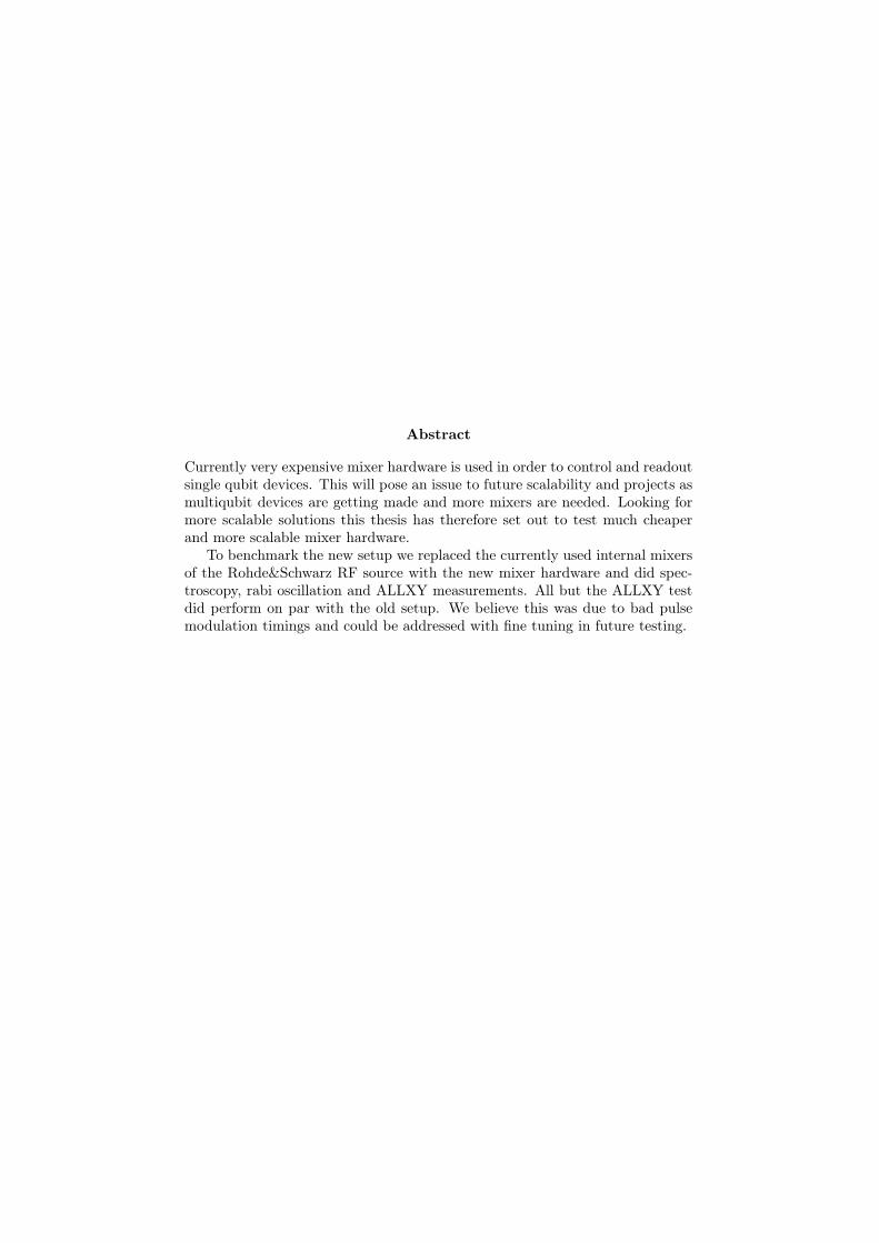
Currently very expensive mixer hardware is used in order to control and readoutsingle qubit devices. This will pose an issue to future scalability and projects asmultiqubit devices are getting made and more mixers are needed. Looking formore scalable solutions this thesis has therefore set out to test much cheaperand more scalable mixer hardware.

To benchmark the new setup we replaced the currently used internal mixersof the Rohde&Schwarz RF source with the new mixer hardware and did spec-troscopy, rabi oscillation and ALLXY measurements. All but the ALLXY testdid perform on par with the old setup. We believe this was due to bad pulsemodulation timings and could be addressed with fine tuning in future testing.

Chapter 1

Introduction

At the heart of all modern day computers, phones and various smart electron-ics lies a central processing unit (CPU), which relies on technology invented ahundred years ago, namely the transistor.

Since the invention, progress of transistor technology has been improvingat a staggering pace, going from big vacuum tubes (1907) to small solid statetransistors (1947) and decreasing their size and increasing their count ever since[1].

Unfortunately this progress is seeming to come to an end as transistor sizeare becoming so small that we are approaching quantum mechanical limits 1.

Though all hope is not lost, it was proposed by Richard Feynman [7] doingcomputations using quantum phenomena, where information is expressed usingqubits instead of classical bits. This would allow for much faster computationsof specific problems as will be discussed in the next section. Much work hasbeen done in the area of quantum computers and multiple propositions has sincebeen made for the underlying technology behind the qubit.

One of these propositions is the superconducting qubit. The advantage ofusing superconducting qubits is scalability as they are very "simple" in natureand can be readily made with current micro fabrication techniques.

This thesis will give an introduction to the theory behind superconductingqubits as discussed in [2] and test out new extensible hardware for use in futurequbit experiments.

1http://www.nature.com/news/the-chips-are-down-for-moore-s-law-1.19338

1

http://www.nature.com/news/the-chips-are-down-for-moore-s-law-1.19338

Chapter 2

Theory

2.1 QubitsTo understand the qubit and why they will bring exponentially faster compu-tation speeds to certain problems, we’ll start by taking a look at the classicalbit (binary digit). The definition of a bit comes from information theory andrepresents one unit of information, which can take one of two values (usually 0or 1). Every bit can therefore only hold one piece of information.

Using multiple bits we can do operations and solve complex mathematicalproblems. One of these problems is prime factorization, which is a problem offiguring out which two prime numbers was used to create a product i.e solvingan equation looking like this prime1 · prime2 = 35.

Now this problem might seem easy and is doable for modern computers,it gets exponentially harder to solve as the product gets larger (try solvingprime1 · prime2 = 445051). The reason why this problem is hard to solve fora computer is basically because the only way for a computer to find the primefactors is simply to try multiplying all combinations of prime numbers until itgets it right.

Lets say you had to solve a 1400 digit product with a modern desktop com-puter it would take about 6.4 quadrillion years to solve1, which is exactly why itsused in RSA-cryptography. It is simply not possible for conventional computersto solve this problem in a reasonably time.

Qubits on the other hand are represented as a quantum mechanical two-state system |ψ〉 = α |1〉+β |2〉 where |ψ〉 is the wave function, |1〉 and |2〉 is thetwo states of the system and α and β are probability amplitudes. Comparedto the classical bit which can only be in one state at a time, a qubit can bein a superposition of two. Adding more qubits allows the system to be ina superposition of multiple states, 2N to be exact where N is the number ofqubits, which means that just by having 500 logical qubits we would be able totest 2500 states at once! This property is exactly why we would be able to solveprime factoring problems infinity faster[6] and why groups around the world arepursuing this technology.

1https://www.digicert.com/TimeTravel/math.htm

2

https://www.digicert.com/TimeTravel/math.htm

2.1.1 The Hydrogen AtomOne natural choice for the physical representation of a qubit would be a hydrogenatom, which is a very well understood system and has exactly the properties weneed. In the hydrogen atom we would use the ground- and first excited state asour qubit. To control the state of our qubit we would shine a laser on the atomwith a frequency equal to the energy difference between |0〉 and |1〉 (∆E = ~ω01

where ω01 is the transition frequency). The laser would then excite the atom toits first excited state and no further because of the anharmonicity of the energylevels figure (2.1). If we keep shining our laser on it, the atom would oscillatebetween |0〉 and |1〉, which is what we call rabi oscillations. Knowing the cycletime of the rabi oscillations allows us to prepare the atom in its first excitedstate or in a superposition between |0〉 and |1〉, by having the laser on for exactlythe amount of time it takes the electron to jump to the desired state.

Now say we prepared the atom in |1〉, we would want to know how longit would stay there, as it would decay because of spontaneous emission. Thisdecay time is often denoted as T1 in literature. Instead lets say we preparedthe atom in a superposition of |0〉 and |1〉, the time in which the system stayscoherent i.e how long can we wait before we no longer measure the superpositionwe prepared it in, is denoted T2*.

[eV]

0.0

|0i

|1i

|2i

Ionization

-13.6

-3.4

-1.51

h!01

|1i ! |0i

h!01

|0i ! |1i

~d~E

Figure 2.1: On the left we see a laser ~E = E0 cos(ω01t) shining on a hydrogen atom whichwill couple with the dipole moment of the atom H = −~d · ~E(t) and stimulate it. On theright we see the energy levels for a hydrogen atom where the laser is stimulating the |0〉 → |1〉transition. Since we don’t turn off the laser the electron will keep going back and forth betweenthe ground- and first exited state which we call rabi oscillations.

3

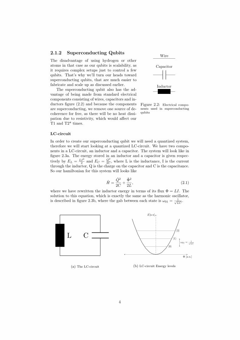
2.1.2 Superconducting QubitsWire

Capacitor

Inductor

Figure 2.2: Electrical compo-nents used in superconductingqubits

The disadvantage of using hydrogen or otheratoms in that case as our qubits is scalability, asit requires complex setups just to control a fewqubits. That’s why we’ll turn our heads towardsuperconducting qubits, that are much easier tofabricate and scale up as discussed earlier.

The superconducting qubit also has the ad-vantage of being made from standard electricalcomponents consisting of wires, capacitors and in-ductors figure (2.2) and because the componentsare superconducting, we remove one source of de-coherence for free, as there will be no heat dissi-pation due to resistivity, which would affect ourT1 and T2* times.

LC-circuit

In order to create our superconducting qubit we will need a quantized system,therefore we will start looking at a quantized LC-circuit. We have two compo-nents in a LC-circuit, an inductor and a capacitor. The system will look like infigure 2.3a. The energy stored in an inductor and a capacitor is given respec-tively by EL = LI2

2 and EC = Q2

2C , where L is the inductance, I is the currentthrough the inductor, Q is the charge on the capacitor and C is the capacitance.So our hamiltonian for this system will looks like

H =Q2

2C+

Φ2

2L, (2.1)

where we have rewritten the inductor energy in terms of its flux Φ = LI. Thesolution to this equation, which is exactly the same as the harmonic oscillator,is described in figure 2.3b, where the gab between each state is ω01 = 1√

LC.

L C

(a) The LC-circuit

E[a.u]

[a.u.]

|0i

|1i

|3i

!01 = 1pLC

(b) LC-circuit Energy levels

4

L C

Mir

crow

ave

sourc

e

(a) Microwave Control capacitivelycoupled with our LC circuit

J C

Mir

crow

ave

sourc

e

(b) Here we replaced the inductor with aJosephson junction

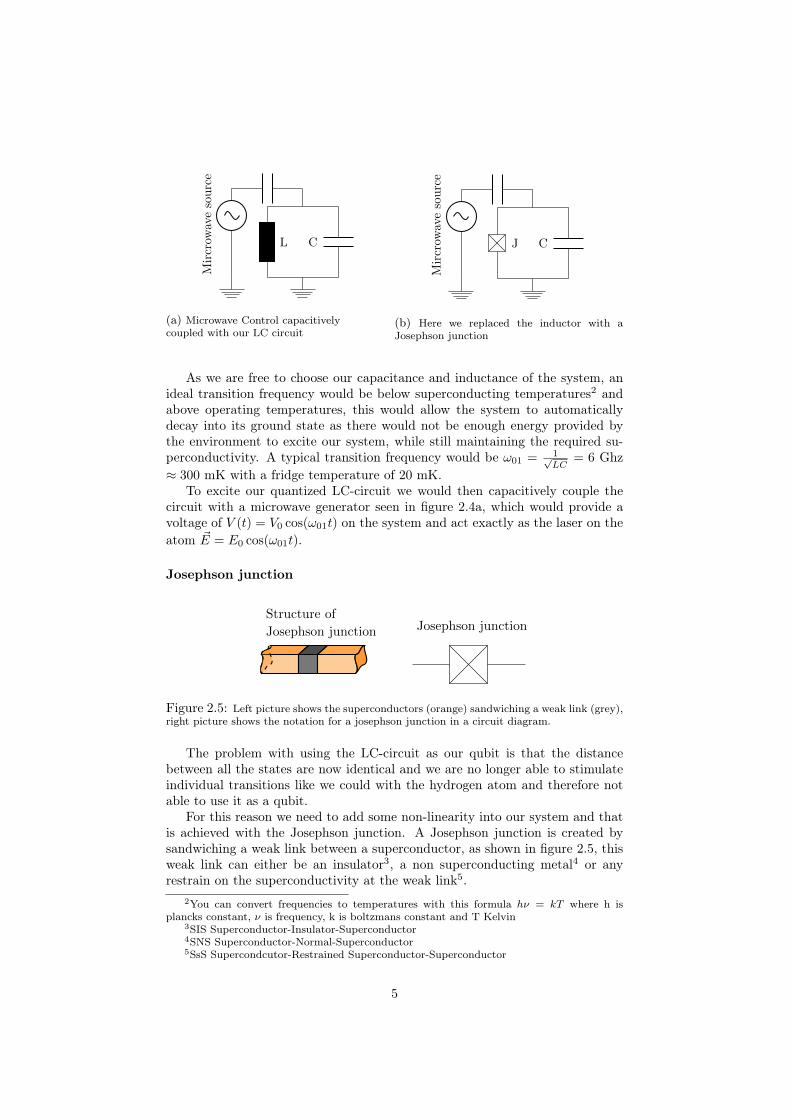
As we are free to choose our capacitance and inductance of the system, anideal transition frequency would be below superconducting temperatures2 andabove operating temperatures, this would allow the system to automaticallydecay into its ground state as there would not be enough energy provided bythe environment to excite our system, while still maintaining the required su-perconductivity. A typical transition frequency would be ω01 = 1√

LC= 6 Ghz

≈ 300 mK with a fridge temperature of 20 mK.To excite our quantized LC-circuit we would then capacitively couple the

circuit with a microwave generator seen in figure 2.4a, which would provide avoltage of V (t) = V0 cos(ω01t) on the system and act exactly as the laser on theatom ~E = E0 cos(ω01t).

Josephson junction

Josephson junctionStructure of

Josephson junction

Figure 2.5: Left picture shows the superconductors (orange) sandwiching a weak link (grey),right picture shows the notation for a josephson junction in a circuit diagram.

The problem with using the LC-circuit as our qubit is that the distancebetween all the states are now identical and we are no longer able to stimulateindividual transitions like we could with the hydrogen atom and therefore notable to use it as a qubit.

For this reason we need to add some non-linearity into our system and thatis achieved with the Josephson junction. A Josephson junction is created bysandwiching a weak link between a superconductor, as shown in figure 2.5, thisweak link can either be an insulator3, a non superconducting metal4 or anyrestrain on the superconductivity at the weak link5.

2You can convert frequencies to temperatures with this formula hν = kT where h isplancks constant, ν is frequency, k is boltzmans constant and T Kelvin

3SIS Superconductor-Insulator-Superconductor4SNS Superconductor-Normal-Superconductor5SsS Supercondcutor-Restrained Superconductor-Superconductor

5

The current though the Josephson junction is given by

I = I0 sin

(2πΦ(t)

Φ0

), (2.2)

where I0 is the supercritical current through the junction and Φ0 = h2e is the

magnetic flux quantum.Taking the time derivative of 2.2 we get

I = I02π

Φ0Φ cos

(2πΦ

Φ0

), (2.3)

where Φ = V (t) and self-inductance is given by L = V (t)

I.

We can then define the Josephson inductance as

LJ =Φ0

2πI0

1

cos(2πΦ/Φ0). (2.4)

The Josephson junction therefore acts as a non-linear inductor. If we re-member from (2.1), the energy stored in the inductor is proportional to 1

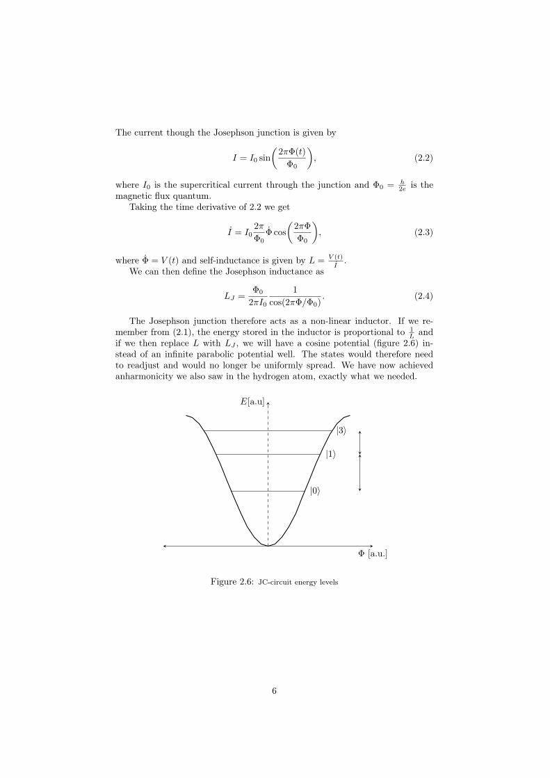
L andif we then replace L with LJ , we will have a cosine potential (figure 2.6) in-stead of an infinite parabolic potential well. The states would therefore needto readjust and would no longer be uniformly spread. We have now achievedanharmonicity we also saw in the hydrogen atom, exactly what we needed.

E[a.u]

[a.u.]

|0i

|1i

|3i

Figure 2.6: JC-circuit energy levels

6

2.2 The Cooper Pair BoxGoing back to the LC-circuit for a moment we can rewrite (2.1) using ω01 = 1√

LC

H =Q2

2C+

1

2Cω01Φ2. (2.5)

Recognizing this as the quantum harmonic oscillator, where P is equivalentto Q and x to Φ, the first term is describing the kinetic energy and the sec-ond term the potential. Therefore the commutation relations we know from thequantum harmonic oscillator, will also apply here. To diagonalize the hamilto-nian we introduce a† and a, as with the quantum harmonic oscillator. Q and Φcan therefore be written as

Q = i

√~

2z0(a† − a), (2.6)

Φ =

√~z0

2(a† + a), (2.7)

where z0 =√

LC .

Plugging these expressions back in 2.5 we get

H = ~ω01(a†a+1

2), (2.8)

which again is the same result as the quantum harmonic oscillator.Now we can do the same calculation for the JC-circuit, but we first have to

find the energy in the Josephson junction. We already know that the currentgoing through the junction is given by (2.2) and we know that the energy is thetime integral of the power therefore

E =

∫P (t)dt =

∫V (t)I(t)dt =

∫(dΦ

dt)(I0 sin

(2πΦ

Φ0

))dt

= −Ej cos

(2πΦ

Φ0

) (2.9)

where EJ = I02πΦ0

. EJ can be seen as the frequency of the cooper pair tunneling,as seen in figure 2.7a

EJ = Frequency of tunneling

(a) Copper pair tunneling through barrier

J C

EC = Energy needed to put charge

into the JC-Circuit from infinity

(b) Electron put on circuit

Figure 2.7

7

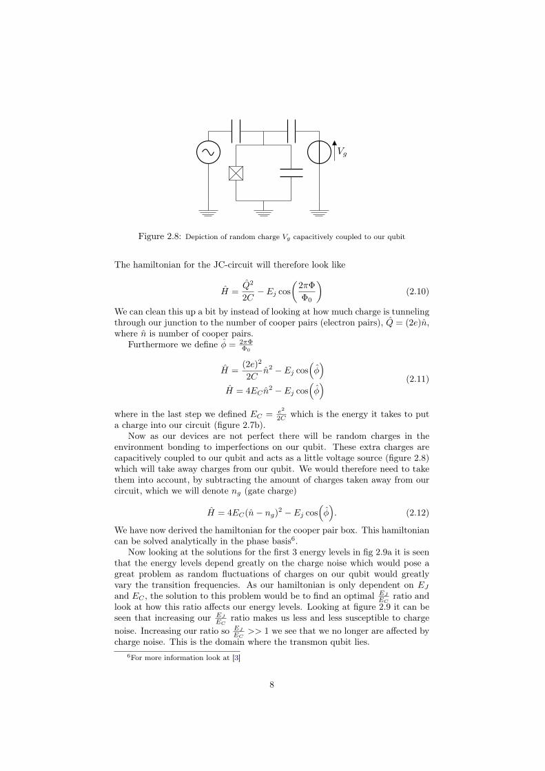
Vg

Figure 2.8: Depiction of random charge Vg capacitively coupled to our qubit

The hamiltonian for the JC-circuit will therefore look like

H =Q2

2C− Ej cos

(2πΦ

Φ0

)(2.10)

We can clean this up a bit by instead of looking at how much charge is tunnelingthrough our junction to the number of cooper pairs (electron pairs), Q = (2e)n,where n is number of cooper pairs.

Furthermore we define φ = 2πΦΦ0

H =(2e)2

2Cn2 − Ej cos

(φ)

H = 4EC n2 − Ej cos

(φ) (2.11)

where in the last step we defined EC = e2

2C which is the energy it takes to puta charge into our circuit (figure 2.7b).

Now as our devices are not perfect there will be random charges in theenvironment bonding to imperfections on our qubit. These extra charges arecapacitively coupled to our qubit and acts as a little voltage source (figure 2.8)which will take away charges from our qubit. We would therefore need to takethem into account, by subtracting the amount of charges taken away from ourcircuit, which we will denote ng (gate charge)

H = 4EC(n− ng)2 − Ej cos(φ). (2.12)

We have now derived the hamiltonian for the cooper pair box. This hamiltoniancan be solved analytically in the phase basis6.

Now looking at the solutions for the first 3 energy levels in fig 2.9a it is seenthat the energy levels depend greatly on the charge noise which would pose agreat problem as random fluctuations of charges on our qubit would greatlyvary the transition frequencies. As our hamiltonian is only dependent on EJand EC , the solution to this problem would be to find an optimal EJ

ECratio and

look at how this ratio affects our energy levels. Looking at figure 2.9 it can beseen that increasing our EJ

ECratio makes us less and less susceptible to charge

noise. Increasing our ratio so EJ

EC>> 1 we see that we no longer are affected by

charge noise. This is the domain where the transmon qubit lies.6For more information look at [3]

8

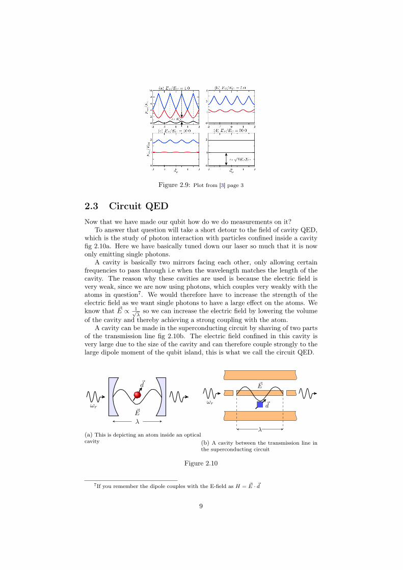
Figure 2.9: Plot from [3] page 3

2.3 Circuit QEDNow that we have made our qubit how do we do measurements on it?

To answer that question will take a short detour to the field of cavity QED,which is the study of photon interaction with particles confined inside a cavityfig 2.10a. Here we have basically tuned down our laser so much that it is nowonly emitting single photons.

A cavity is basically two mirrors facing each other, only allowing certainfrequencies to pass through i.e when the wavelength matches the length of thecavity. The reason why these cavities are used is because the electric field isvery weak, since we are now using photons, which couples very weakly with theatoms in question7. We would therefore have to increase the strength of theelectric field as we want single photons to have a large effect on the atoms. Weknow that ~E ∝ 1√

λso we can increase the electric field by lowering the volume

of the cavity and thereby achieving a strong coupling with the atom.A cavity can be made in the superconducting circuit by shaving of two parts

of the transmission line fig 2.10b. The electric field confined in this cavity isvery large due to the size of the cavity and can therefore couple strongly to thelarge dipole moment of the qubit island, this is what we call the circuit QED.

~E

!r

~d

(a) This is depicting an atom inside an opticalcavity

!r ~d

~E

(b) A cavity between the transmission line inthe superconducting circuit

Figure 2.10

7If you remember the dipole couples with the E-field as H = ~E · ~d

9

Figure 2.11: Diagram of the full transmon qubit circuit

2.4 Jaynes-Cummings HamiltonianAs the cavity only allows for certain resonance frequencies i.e only certain en-ergies are allowed, it will behave as the harmonic LC-circuit. Bringing all thatwe have learned until now together, we can write the hamiltonian as a sum ofthe LC- and JC-circuit

H =Q2r

2Cr+

Φ2r

2Lr︸︷︷︸LC−circuit

+ 4EC(n− ng)2 − Ej cos(φ)

︸︷︷︸JC−circuit

, (2.13)

H = ~ωr(a†a+1

2) +

~ω01

2σz + ~g(a†σ−︸︷︷︸

create

+ aσ+︸︷︷︸annihilate

), 8 (2.14)

where ωr and ω01 respectively is the cavity resonance frequency and the qubitfrequency, a† and a the raising and lowering operators, σz the Pauli spin matrixoperator, g = ~E · ~d the qubit-cavity coupling strength and finally σ+ and σ−the spin raising and lowering operators.

The create term in (2.14) can be seen as a photon created by the loweringoperator that will then jump to the cavity, where the annihilate term will removea photon from the cavity by exiting the qubit.

2.5 Dispersive Regime: Qubit ReadoutQubit readout can be done by working in the dispersive regime of the Jaynes-Cummings hamilton i.e |∆| = |ω01 − ωr| g. Here the Jaynes-Cummingshamilton will reduce to

H ≈ (ωr + χ)a†a+ω01

2σz, (2.15)

where χ = g2

∆ .Now we can se that the cavity transmission frequency depends on the state

of the qubit, so if the qubit is in the ground state the cavity frequency willbe shifted down and if the qubit is in its exited state be pulled up, as can beseen in figure 2.12. This principle is used to determine the state of the qubit inexperiments.

8A more detailed derivation can be found in [4].

10

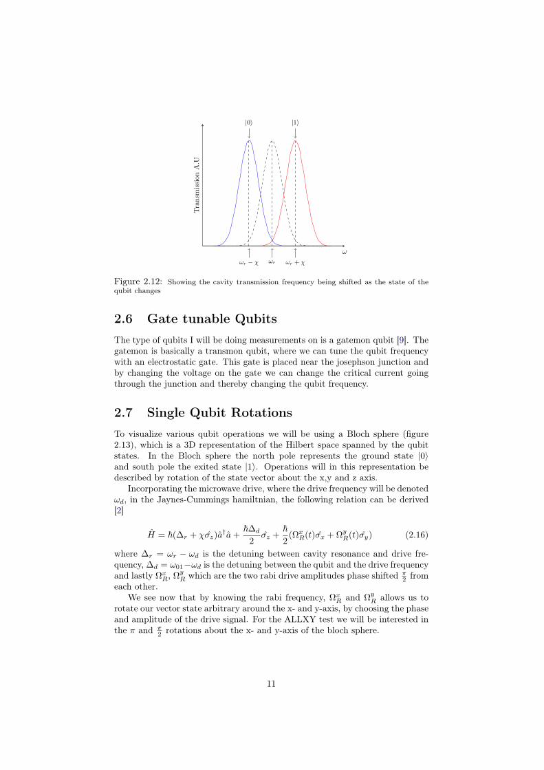
|0i |1i

!r !r + !r

Tra

nsm

issi

onA

.U

!

1

Figure 2.12: Showing the cavity transmission frequency being shifted as the state of thequbit changes

2.6 Gate tunable QubitsThe type of qubits I will be doing measurements on is a gatemon qubit [9]. Thegatemon is basically a transmon qubit, where we can tune the qubit frequencywith an electrostatic gate. This gate is placed near the josephson junction andby changing the voltage on the gate we can change the critical current goingthrough the junction and thereby changing the qubit frequency.

2.7 Single Qubit RotationsTo visualize various qubit operations we will be using a Bloch sphere (figure2.13), which is a 3D representation of the Hilbert space spanned by the qubitstates. In the Bloch sphere the north pole represents the ground state |0〉and south pole the exited state |1〉. Operations will in this representation bedescribed by rotation of the state vector about the x,y and z axis.

Incorporating the microwave drive, where the drive frequency will be denotedωd, in the Jaynes-Cummings hamiltnian, the following relation can be derived[2]

H = ~(∆r + χσz)a†a+

~∆d

2σz +

~2

(ΩxR(t)σx + ΩyR(t)σy) (2.16)

where ∆r = ωr − ωd is the detuning between cavity resonance and drive fre-quency, ∆d = ω01−ωd is the detuning between the qubit and the drive frequencyand lastly ΩxR, ΩyR which are the two rabi drive amplitudes phase shifted π

2 fromeach other.

We see now that by knowing the rabi frequency, ΩxR and ΩyR allows us torotate our vector state arbitrary around the x- and y-axis, by choosing the phaseand amplitude of the drive signal. For the ALLXY test we will be interested inthe π and π

2 rotations about the x- and y-axis of the bloch sphere.

11

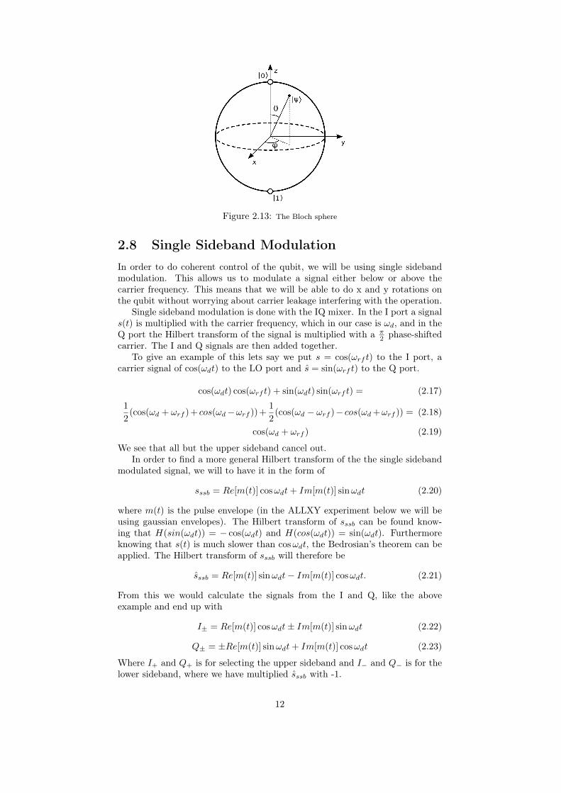
Figure 2.13: The Bloch sphere

2.8 Single Sideband ModulationIn order to do coherent control of the qubit, we will be using single sidebandmodulation. This allows us to modulate a signal either below or above thecarrier frequency. This means that we will be able to do x and y rotations onthe qubit without worrying about carrier leakage interfering with the operation.

Single sideband modulation is done with the IQ mixer. In the I port a signals(t) is multiplied with the carrier frequency, which in our case is ωd, and in theQ port the Hilbert transform of the signal is multiplied with a π

2 phase-shiftedcarrier. The I and Q signals are then added together.

To give an example of this lets say we put s = cos(ωrf t) to the I port, acarrier signal of cos(ωdt) to the LO port and s = sin(ωrf t) to the Q port.

cos(ωdt) cos(ωrf t) + sin(ωdt) sin(ωrf t) = (2.17)

1

2(cos(ωd + ωrf ) + cos(ωd−ωrf )) +

1

2(cos(ωd − ωrf )− cos(ωd+ωrf )) = (2.18)

cos(ωd + ωrf ) (2.19)

We see that all but the upper sideband cancel out.In order to find a more general Hilbert transform of the the single sideband

modulated signal, we will to have it in the form of

sssb = Re[m(t)] cosωdt+ Im[m(t)] sinωdt (2.20)

where m(t) is the pulse envelope (in the ALLXY experiment below we will beusing gaussian envelopes). The Hilbert transform of sssb can be found know-ing that H(sin(ωdt)) = − cos(ωdt) and H(cos(ωdt)) = sin(ωdt). Furthermoreknowing that s(t) is much slower than cosωdt, the Bedrosian’s theorem can beapplied. The Hilbert transform of sssb will therefore be

sssb = Re[m(t)] sinωdt− Im[m(t)] cosωdt. (2.21)

From this we would calculate the signals from the I and Q, like the aboveexample and end up with

I± = Re[m(t)] cosωdt± Im[m(t)] sinωdt (2.22)

Q± = ±Re[m(t)] sinωdt+ Im[m(t)] cosωdt (2.23)

Where I+ and Q+ is for selecting the upper sideband and I− and Q− is for thelower sideband, where we have multiplied sssb with -1.

12

Chapter 3

Setup

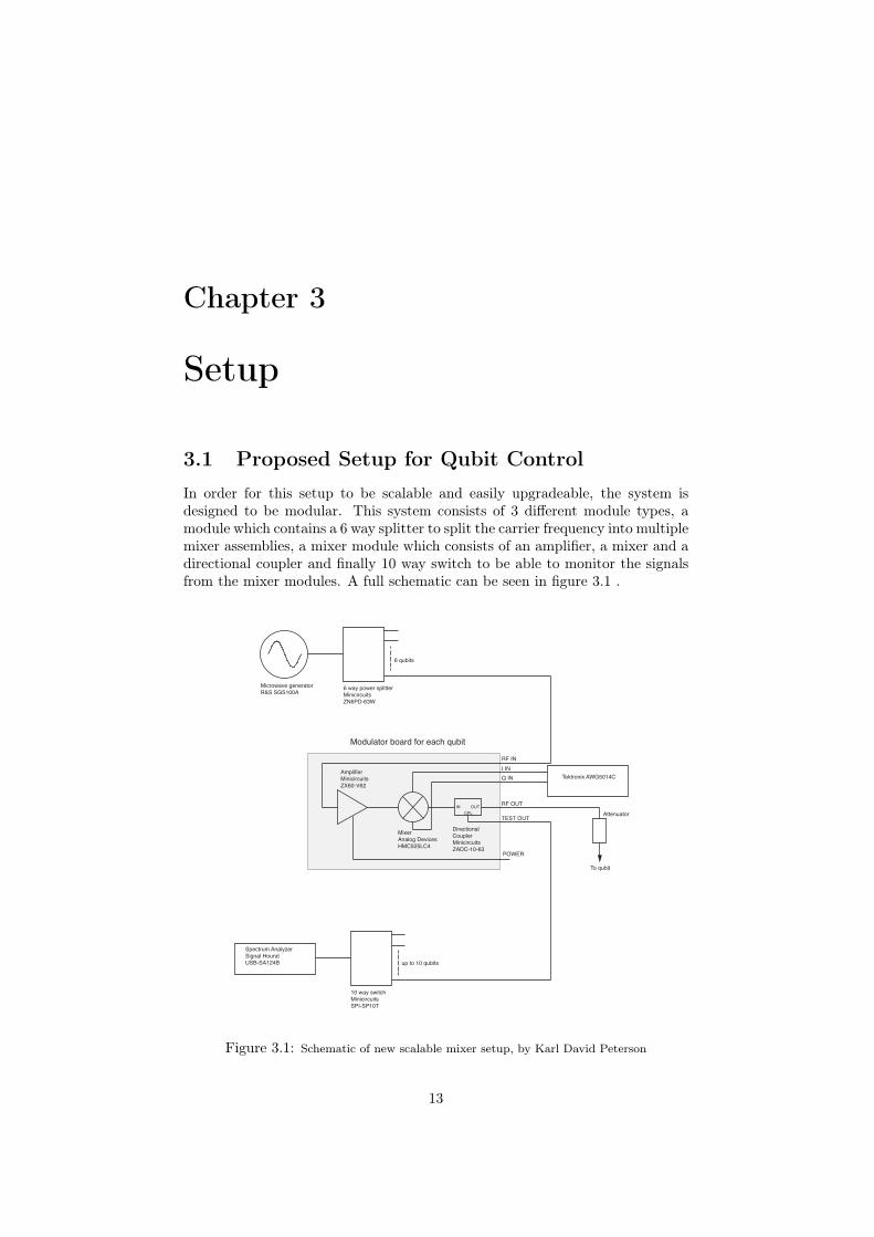
3.1 Proposed Setup for Qubit ControlIn order for this setup to be scalable and easily upgradeable, the system isdesigned to be modular. This system consists of 3 different module types, amodule which contains a 6 way splitter to split the carrier frequency into multiplemixer assemblies, a mixer module which consists of an amplifier, a mixer and adirectional coupler and finally 10 way switch to be able to monitor the signalsfrom the mixer modules. A full schematic can be seen in figure 3.1 .

6 way power splitterMinicircuitsZN6PD-63W

6 qubits

AmplifierMinicircuitsZX60-V62

MixerAnalog DevicesHMC525LC4

RF INI INQ IN

IN OUTCPL

RF OUT

TEST OUT

POWER

Tektronix AWG5014C

Attenuator

To qubit

DirectionalCouplerMinicircuitsZADC-10-63

10 way switchMinicircuitsSPI-SP10T

up to 10 qubits

Microwave generatorR&S SGS100A

Spectrum AnalyzerSignal HoundUSB-SA124B

Modulator board for each qubit

Figure 3.1: Schematic of new scalable mixer setup, by Karl David Peterson

13

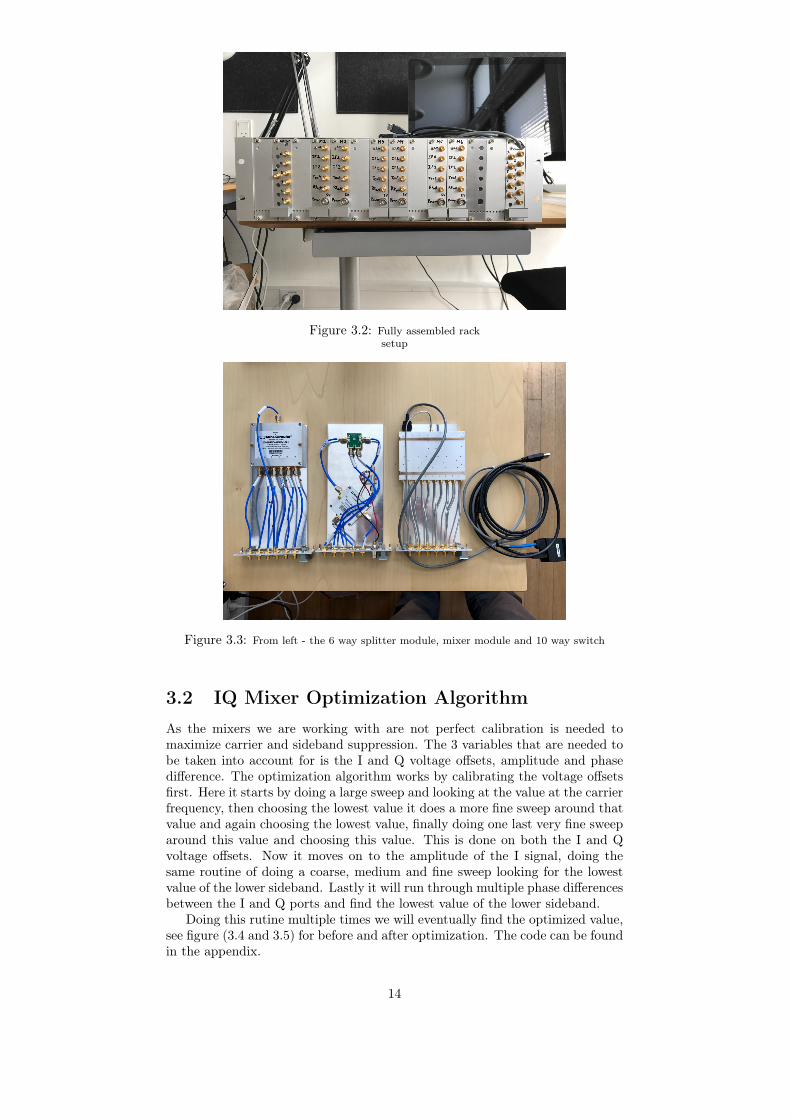
Figure 3.2: Fully assembled racksetup

Figure 3.3: From left - the 6 way splitter module, mixer module and 10 way switch

3.2 IQ Mixer Optimization AlgorithmAs the mixers we are working with are not perfect calibration is needed tomaximize carrier and sideband suppression. The 3 variables that are needed tobe taken into account for is the I and Q voltage offsets, amplitude and phasedifference. The optimization algorithm works by calibrating the voltage offsetsfirst. Here it starts by doing a large sweep and looking at the value at the carrierfrequency, then choosing the lowest value it does a more fine sweep around thatvalue and again choosing the lowest value, finally doing one last very fine sweeparound this value and choosing this value. This is done on both the I and Qvoltage offsets. Now it moves on to the amplitude of the I signal, doing thesame routine of doing a coarse, medium and fine sweep looking for the lowestvalue of the lower sideband. Lastly it will run through multiple phase differencesbetween the I and Q ports and find the lowest value of the lower sideband.

Doing this rutine multiple times we will eventually find the optimized value,see figure (3.4 and 3.5) for before and after optimization. The code can be foundin the appendix.

14

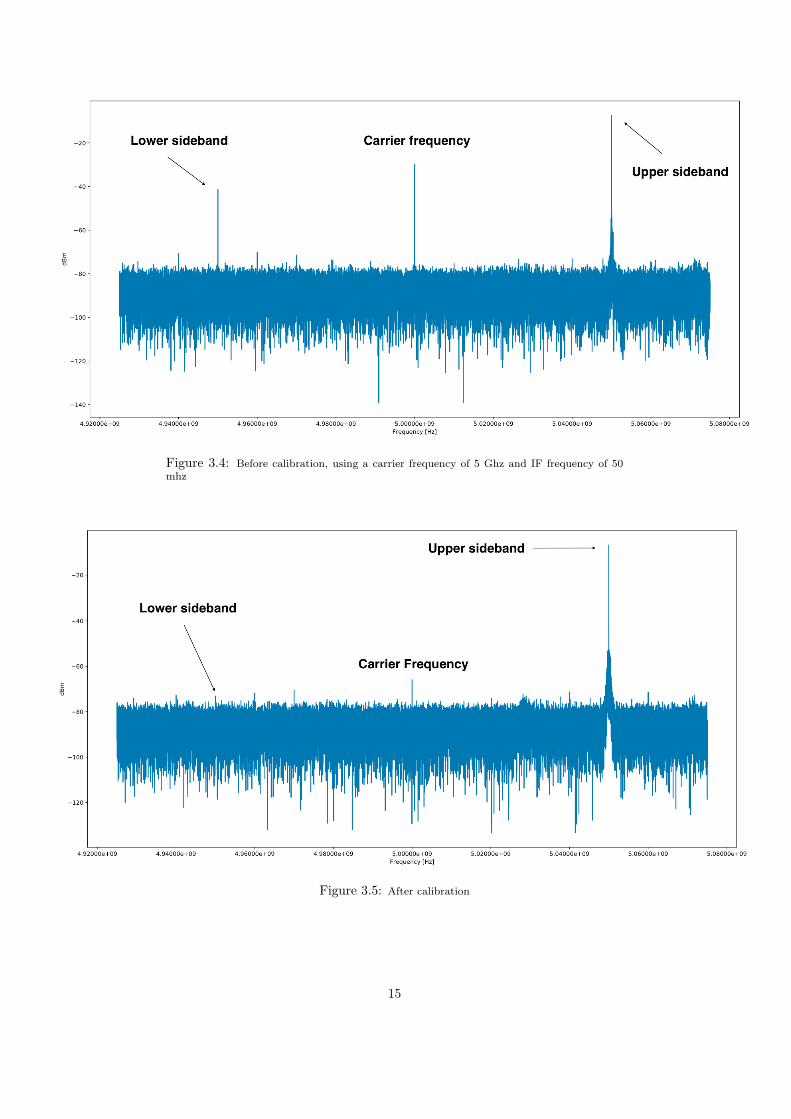
Figure 3.4: Before calibration, using a carrier frequency of 5 Ghz and IF frequency of 50mhz

Figure 3.5: After calibration

15

Chapter 4

Experiment

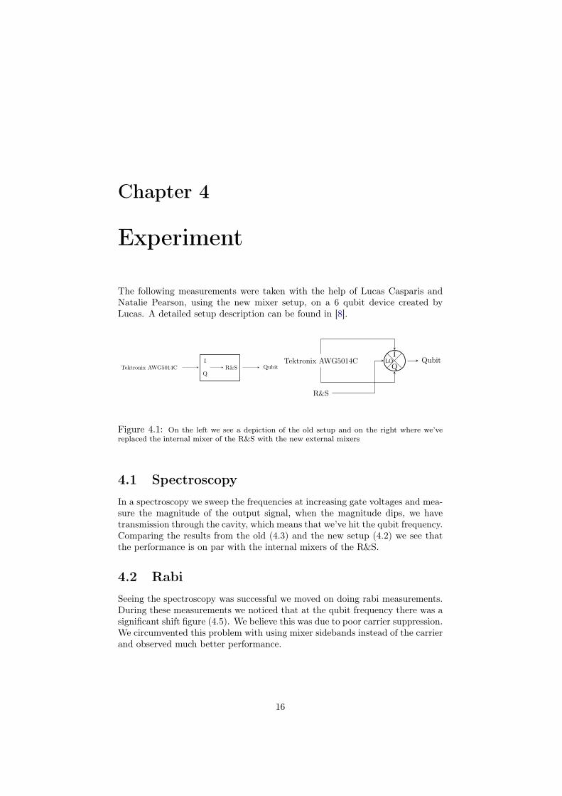
The following measurements were taken with the help of Lucas Casparis andNatalie Pearson, using the new mixer setup, on a 6 qubit device created byLucas. A detailed setup description can be found in [8].

Tektronix AWG5014CI

QR&S Qubit

Tektronix AWG5014CI

QLO

R&S

Qubit

Figure 4.1: On the left we see a depiction of the old setup and on the right where we’vereplaced the internal mixer of the R&S with the new external mixers

4.1 SpectroscopyIn a spectroscopy we sweep the frequencies at increasing gate voltages and mea-sure the magnitude of the output signal, when the magnitude dips, we havetransmission through the cavity, which means that we’ve hit the qubit frequency.Comparing the results from the old (4.3) and the new setup (4.2) we see thatthe performance is on par with the internal mixers of the R&S.

4.2 RabiSeeing the spectroscopy was successful we moved on doing rabi measurements.During these measurements we noticed that at the qubit frequency there was asignificant shift figure (4.5). We believe this was due to poor carrier suppression.We circumvented this problem with using mixer sidebands instead of the carrierand observed much better performance.

16

Figure 4.2: Spectroscopy using new mixer setup

Figure 4.3: Spectroscopy using old mixer setup

17

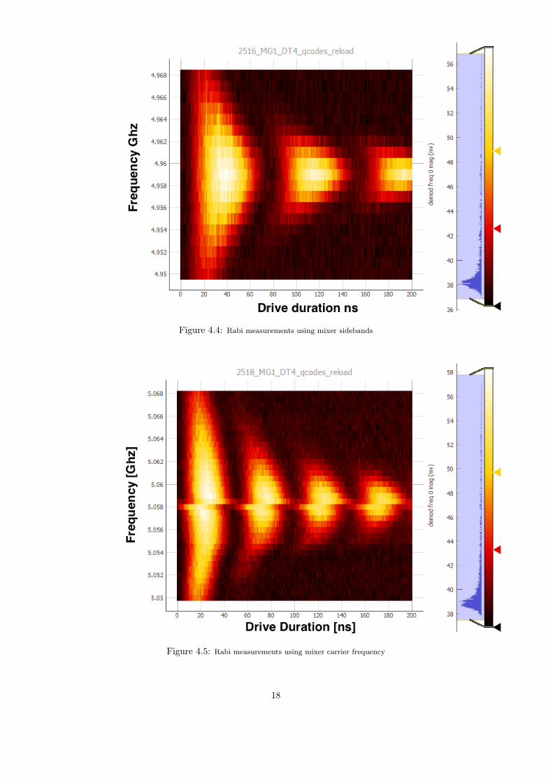
Figure 4.4: Rabi measurements using mixer sidebands

Figure 4.5: Rabi measurements using mixer carrier frequency

18

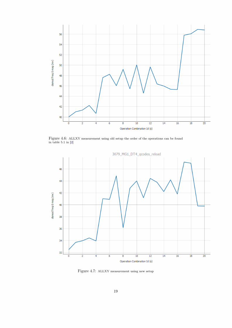
Figure 4.6: ALLXY measurement using old setup the order of the operations can be foundin table 5.1 in [2]

Figure 4.7: ALLXY measurement using new setup

19

4.3 Gate tuneup / ALLXYFinally we tried to tune the qubits doing an ALLXY test. In an ALLXY test allcombinations of one and two π,pi2 rotations, about both the x- and y-axis areperformed. By looking at the measurements deviation from the expected values,different error types can be identified and accounted for. In this experimentwe used single sideband modulated gaussian pulses. All the combinations ofoperations and more detailed description can be found in [2] where the order ofour operations can be found in table 5.1.

We first did the ALLXY measurements using the old setup to get a baselineon how good we could tune the qubit. Looking at a line cut in figure 4.6 itwas pretty good, as the measurements fit the expected values when doing thevarious operation combinations. Now changing to the new setup we did not seesame success as can be seen in figure 4.7.

We can see from the line cut that doing a π rotation (operation 19 and 20)is not getting the same result as doing two π

2 rotations (operation 17 and 18).This indicates that our x and y gates are not perfectly π

2 shifted from each otherand would therefore cause under rotation in the Bloch sphere. This could beaddressed by fine tuning of phase difference between the sideband modulatedpulses, unfortunately time ran out and could therefore be a calibration to tryin future experiments.

4.4 ConclusionFrom these results we can conclude that this new setup looks very promising,though further tuneup would be needed in order to match the performance ofthe R&S.

This proof of concept opens up new possibilities for future multi qubit ex-periments, as it is now shown that much cheaper hardware allows for similarperformance as current setups. To further improve the scalability and reducecosts of this setup, one could consider creating a integrated circuit with mixers,amplifiers and decouplers build in.

20

Bibliography

[1] Gordon E. Moore Cramming more components onto integrated circuitsElectronics, volume 38, number 8, April 19, 1965, pp.114 ff.

[2] Matthew David Reed Entanglement and Quantum Error Correction withSuperconducting Qubits

[3] Jens Koch, Terri M. Yu, Jay Gambetta, A. A. Houck, D. I. Schuster, J.Majer, Alexandre Blais, M. H. Devoret, S. M. Girvin, R. J. SchoelkopfCharge insensitive qubit design derived from the Cooper pair box Phys.Rev. A 76, 042319 (2007)

[4] Alexandre Blais, Ren-Shou Huang, Andreas Wallraff, S. M. Girvin, andR. J. Schoelkopf Cavity quantum electrodynamics for superconducting elec-trical circuits: An architecture for quantum computation PHYSICAL RE-VIEW A 69, 062320 (2004)

[5] T.W. Larsen, K.D. Peterson, F. Kuemmeth, T.S Jespersen, P. Krogstrup, J.Nygaard and C.M. Marcus Semicondcutor-Nanowire-Based Superconduct-ing Qubit Phys. Rev. Lett. 115, 127001 – Published 14 September 2015

[6] Peter W. Shor Algorithms for Quantum Computation: Discrete Logarithmsand Factoring Proc. 35nd Annual Symposium on Foundations of ComputerScience (Shafi Goldwasser, ed.), IEEE Computer Society Press (1994), 124-134.

[7] Richard P. Feynman Simulating Physics with Computers InternationalJournal of Theoretical Physics, VoL 21, Nos.6/7, 1982

[8] Anders Kringhøj Readout and Control of Semiconductor- Nanowire-BasedSuperconducting Qubits

[9] Blake Robert Johnson Controlling photons in superconducting electrical cir-cuits

21

Appendix A

Mixer OptimizationAlgorithm Code

22

AWG Automation initialiser

June 11, 2017

In [1]: '''Initialize the AWG'''

import osimport timeimport logging

import numpy as npimport matplotlib.pyplot as plt

logger = logging.getLogger()logger.setLevel(logging.INFO)

import qcodes.instrument_drivers.tektronix.AWG5014 as awg # <--- The instrument driverfrom qcodes.instrument_drivers.tektronix.AWGFileParser import parse_awg_file # <--- A helper function

awg1 = awg.Tektronix_AWG5014('AWG1', 'TCPIP0::172.20.3.14::inst0::INSTR', timeout=40)

AWG clock freq not set to 1GHz

Connected to: 1.20000000E+009 None (serial:None, firmware:None) in 0.08s

In [2]: #Set the amplitude of used channels to not destroy the IQ mixer

awg1.clock_freq(1e9)

current_amp = 0.2

awg1.ch1_amp.set(current_amp)awg1.ch2_amp.set(current_amp)

awg1.ch1_offset.set(0)

awg1.ch2_offset.set(0)

In [3]: # noofseqelems runs all the different waveforms after each other in the waveformgeneratornoofseqelems = 50

1

noofpoints = 2001band_frequency = 50e6

waveforms = [[], []] # one list for each channelm1s = [[], []]m2s = [[], []]for ii in range(noofseqelems):

# waveform and markers for channel 1#Remember that i put 2 times in to get right mode

wf0 = np.sin(2*np.pi*np.linspace(0, 2000 , noofpoints) * (band_frequency * 1e-9) - ii*0.1*(np.pi / 180) - 90 * np.pi / 180)wf0 = np.delete(wf0, int(noofpoints-1))waveforms[0].append(wf0)

# waveforms[0].append(np.sin(2*np.pi*(ii+1)*np.linspace(0, 1 , noofpoints)))#waveforms[0] = np.delete(waveforms[0], int(noofpoints-1))

m1 = np.zeros(noofpoints-1)m1[:int((noofpoints-1)/(ii+1))] = 1m1s[0].append(m1)m2 = np.zeros(noofpoints-1)m2s[0].append(m2)

# waveform and markers for channel two#Remember that i put 2 times in to get right modewf = np.sin(2*np.pi*np.linspace(0, 2000, noofpoints) * band_frequency * 1e-9)wf = np.delete(wf, int(noofpoints-1))waveforms[1].append(wf)

m1 = np.zeros(noofpoints-1)m1[:int(noofpoints-1/(ii+1))] = 1m1s[1].append(m1)m2 = np.zeros(noofpoints-1)m2s[1].append(m2)

In [6]: # number of repetitionsnreps = [0 for ii in range(noofseqelems)]

trig_waits = [0]*noofseqelems# Goto stategoto_states = [0]*noofseqelems# Event jumpjump_tos = [0]*noofseqelems

awg1.make_send_and_load_awg_file(waveforms, m1s, m2s,nreps, trig_waits,

2

goto_states, jump_tos, channels=[1, 2])

In [5]: awg1.clear_message_queue()

In [7]: awg1.all_channels_on()awg1.run()

Out[7]: 'Running'

In [8]: import qcodes.instrument_drivers.signal_hound.USB_SA124B as shimport matplotlib.pyplot as plt

''' Here you specify the path to your sa_api.dll filewhich is located in the signal hound install folder. '''

sa_api_path = 'C:\Program Files\Signal Hound\Spike\sa_api.dll' # Specify here between the apostrophe

sh1 = sh.SignalHound_USB_SA124B('sh1', sa_api_path)

INFO:root:qcodes.instrument_drivers.signal_hound.USB_SA124B : Initializing instrument SignalHound USB 124AINFO:Main.DeviceInt:Opening DeviceINFO:Main.DeviceInt:Querying device for model informationINFO:Main.DeviceInt:Querying device for model information

Initialized SignalHound in 6.83s

In [242]: ''' Specify the frequency and span to sweep accros in hz '''

#Specify frequencyfrequency = 4.85e9sh1.frequency(frequency)

#Specify Spanspan = 100e6#span = 10e3sh1.span(span)

#This updates the frequency and span parameters and prepares the device for measurementsh1.prepare_for_measurement()

'''Determine whether or not you want to plot your sweeped span'''

plot_or_not = 'yes' #yes or no between the apostrophe

3

if plot_or_not == 'yes':spectrum = sh1.sweep() #Sweeps the desired range and returns like this, np.array([freq_points, datamin, datamax])

fig = plt.figure(figsize=(20,10))ax = fig.add_subplot(111)plt.plot(spectrum[0], spectrum[1]) #Plots dBm vs frequencyax.xaxis.set_major_formatter(plt.FormatStrFormatter('%.5e'))plt.ylabel('dBm')plt.xlabel('Frequency [Hz]')plt.show()

'''If you only want the power at the specified frequency'''

power_at_freq = sh1.get_power_at_freq()

print('Power at %.2e [Hz] is %.2f [dBm]' % (sh1.get('frequency'), power_at_freq))

INFO:Main.DeviceInt:Setting device CenterSpan configuration.INFO:Main.DeviceInt:Setting device reference level configuration.INFO:Main.DeviceInt:Setting device Sweeping configuration.

Warning: saBandwidthClamped

Power at 4.85e+09 [Hz] is -53.07 [dBm]

In [235]: import timestart_time = time.clock()

#Initialize the spectrum analysersh1.frequency(frequency)sh1.span(10e3)sh1.prepare_for_measurement()

#Initialize sweep for channel1a = []ch1_offset = 0.03

#Initialize sweep for channel2b = []ch2_offset = 0.03

4

t = 0################################################################################################################################while t <= 15:

awg1.ch1_offset.set(ch1_offset)time.sleep(0.4)power = sh1.get_power_at_freq()

a.append([ch1_offset, power])ch1_offset += -0.004

t += 1

#Finds the minimum in a and returns the offset value for this minimumg = round(min((i for i in a), key=lambda i: i[1])[0],3)

a = []ch1_offset = g + 0.004

t = 0

while t <= 8:awg1.ch1_offset.set(ch1_offset)time.sleep(0.4)power = sh1.get_power_at_freq()

a.append([ch1_offset, power])ch1_offset += -0.001

t += 1

g = round(min((i for i in a), key=lambda i: i[1])[0],3)awg1.ch1_offset.set(g)

################################################################################################################################t = 0

while t <= 15:awg1.ch2_offset.set(ch2_offset)time.sleep(0.4)power = sh1.get_power_at_freq()b.append([ch2_offset, power])

ch2_offset += -0.004

t += 1

5

#Finds the minimum in a and returns the offset value for this minimumh = round(min((i for i in b), key=lambda i: i[1])[0],3)

b = []ch2_offset = h + 0.004

t = 0

while t <= 8:awg1.ch2_offset.set(ch2_offset)time.sleep(0.4)power = sh1.get_power_at_freq()b.append([ch2_offset, power])

ch2_offset += -0.001

t += 1

h = round(min((i for i in b), key=lambda i: i[1])[0],3)awg1.ch2_offset.set(h)

################################################################################################################################

print((time.clock() - start_time), "seconds")

INFO:Main.DeviceInt:Setting device CenterSpan configuration.INFO:Main.DeviceInt:Setting device reference level configuration.INFO:Main.DeviceInt:Setting device Sweeping configuration.INFO:Main.DeviceInt:Call to initiate succeeded.

30.333558417165477 seconds


#Initialize the spectrum analysersh1.frequency(frequency - band_frequency)sh1.span(10e3)sh1.prepare_for_measurement()

6

time.sleep(1)

#Initialize sweep for channel1a = []ch1_amplitude = current_amp + 0.100

t = 0################################################################################################################################

while t <= 5:awg1.ch1_amp.set(ch1_amplitude)time.sleep(0.5)power = sh1.get_power_at_freq()a.append([ch1_amplitude, power])

ch1_amplitude += -0.04

t += 1

#Finds the minimum in a and returns the offset value for this minimumg = min((i for i in a), key=lambda i: i[1])[0]awg1.ch1_amp.set(g + 0.04)

################################################ new parta = []ch1_amplitude = g + 0.04

t = 0



t += 1

g = min((i for i in a), key=lambda i: i[1])[0]awg1.ch1_amp.set(g + 0.008)

################################################################################################################################

a = []ch1_amplitude = g + 0.008

7

t = 0



t += 1

g = min((i for i in a), key=lambda i: i[1])[0]awg1.ch1_amp.set(g)



21.32087232743106 seconds


#Initialize the spectrum analysersh1.frequency(frequency - band_frequency)sh1.span(10e3)sh1.prepare_for_measurement()

#Initialize sweep for channel1a = []seq_pos = 1

t = 0

while t < noofseqelems:awg1.sequence_pos.set(seq_pos)time.sleep(0.5)power = sh1.get_power_at_freq()

a.append([seq_pos, power])seq_pos += 1

8

t += 1

#Finds the minimum in a and returns the offset value for this minimumg = min((i for i in a), key=lambda i: i[1])[0]awg1.sequence_pos.set(g)



35.099577999888425 seconds

In [240]: np.savetxt('C:\\Users\\Triton 5 DAQ\\Desktop\\daniel\\5ghz_50mhz_RS25dbm_HM1000a.txt', spectrum)

In [7]: import numpy as np

In [128]: power

Out[128]: -45.067314147949219

In [243]: low = power_at_freq

In [241]: high = power_at_freq

In [244]: delta = high - low

In [245]: delta

Out[245]: 53.076743410667405

In [153]: low

Out[153]: -54.266780853271484

In [ ]:

9

Extensible hardware for control of superconducting qubits · 2017-06-21 · Chapter 2 Theory 2.1...

Documents

Transcript of Extensible hardware for control of superconducting qubits · 2017-06-21 · Chapter 2 Theory 2.1...