EXPERIMENTS ON SUPERCONDUCTING JOSEPHSON PHASE QUANTUM BITS · 1.3 Quantum computation ... 3.6.4...
128
E XPERIMENTS ON SUPERCONDUCTING J OSEPHSON P HASE Q UANTUM B ITS Den Naturwissenschaftlichen Fakult¨ aten der Friedrich-Alexander-Universit¨ at Erlangen-N ¨ urnberg zur Erlangung des Doktorgrades vorgelegt von J¨ urgen Lisenfeld aus N ¨ urnberg
Transcript of EXPERIMENTS ON SUPERCONDUCTING JOSEPHSON PHASE QUANTUM BITS · 1.3 Quantum computation ... 3.6.4...

EXPERIMENTS ON
SUPERCONDUCTING JOSEPHSON
PHASE QUANTUM BITS
Den Naturwissenschaftlichen Fakultaten derFriedrich-Alexander-Universitat Erlangen-Nurnberg
zur
Erlangung des Doktorgrades
vorgelegt von
Jurgen Lisenfeldaus Nurnberg

Als Dissertation genehmigt von den Naturwissenschaftlichen Fakultaten derUniversitat Erlangen-Nurnberg
Tag der mundlichen Prufung: 19.12.2007
Vorsitzender der Promotionskommission: Prof. Dr. Eberhard Bansch
Erstberichterstatter: Prof. Dr. A. V. Ustinov
Zweitberichterstatter: Prof. Dr. C. Cosmelli

Contents
1 Introduction 11.1 Macroscopic quantum coherence in superconducting circuits . . . . . 11.2 The Josephson phase qubit . . . . . . . . . . . . . . . . . . . . . . . 21.3 Quantum computation . . . . . . . . . . . . . . . . . . . . . . . . . 21.4 Implementation of a quantum computer . . . . . . . . . . . . . . . . 31.5 Outlook . . . . . . . . . . . . . . . . . . . . . . . . . . . . . . . . . 5
2 Principles of the phase qubit 72.1 Superconductivity . . . . . . . . . . . . . . . . . . . . . . . . . . . . 72.2 The current-biased Josephson junction . . . . . . . . . . . . . . . . . 8
2.2.1 Josephson equations . . . . . . . . . . . . . . . . . . . . . . 92.2.2 The RCSJ model . . . . . . . . . . . . . . . . . . . . . . . . 92.2.3 Classical phase dynamics . . . . . . . . . . . . . . . . . . . . 112.2.4 Macroscopic quantum effects . . . . . . . . . . . . . . . . . 132.2.5 Escape mechanisms . . . . . . . . . . . . . . . . . . . . . . 14
2.3 Coherent dynamics in the two-state system . . . . . . . . . . . . . . . 172.3.1 Rabi oscillation . . . . . . . . . . . . . . . . . . . . . . . . . 182.3.2 Energy-level repulsion . . . . . . . . . . . . . . . . . . . . . 222.3.3 Bloch-sphere description of the qubit state . . . . . . . . . . . 232.3.4 Decoherence . . . . . . . . . . . . . . . . . . . . . . . . . . 24
3 The flux-biased phase qubit 273.1 Qubit isolation . . . . . . . . . . . . . . . . . . . . . . . . . . . . . 27
3.1.1 Dissipation in the environment . . . . . . . . . . . . . . . . . 273.1.2 Relaxation rate . . . . . . . . . . . . . . . . . . . . . . . . . 283.1.3 Inductive isolation . . . . . . . . . . . . . . . . . . . . . . . 283.1.4 Isolation by impedance transformation . . . . . . . . . . . . . 29
3.2 rf-SQUID principles . . . . . . . . . . . . . . . . . . . . . . . . . . 303.2.1 Potential energy . . . . . . . . . . . . . . . . . . . . . . . . 303.2.2 Energy levels . . . . . . . . . . . . . . . . . . . . . . . . . . 333.2.3 Escape rates . . . . . . . . . . . . . . . . . . . . . . . . . . . 35
3.3 Qubit operation . . . . . . . . . . . . . . . . . . . . . . . . . . . . . 373.4 Readout . . . . . . . . . . . . . . . . . . . . . . . . . . . . . . . . . 38
3.4.1 Principles of the dc-SQUID . . . . . . . . . . . . . . . . . . 383.4.2 Switching-current readout . . . . . . . . . . . . . . . . . . . 41
3.5 Sample design . . . . . . . . . . . . . . . . . . . . . . . . . . . . . . 453.5.1 Niobium - SiOx - based standard fabrication processes . . . . 453.5.2 Sample parameters and nomenclature . . . . . . . . . . . . . 48
i
3.5.3 Al - SiN - based samples from UCSB . . . . . . . . . . . . . 493.6 Experimental technique . . . . . . . . . . . . . . . . . . . . . . . . . 50
3.6.1 Wiring and filtering . . . . . . . . . . . . . . . . . . . . . . . 503.6.2 Sample holder . . . . . . . . . . . . . . . . . . . . . . . . . 513.6.3 Electronics . . . . . . . . . . . . . . . . . . . . . . . . . . . 513.6.4 Microwave pulse modulation . . . . . . . . . . . . . . . . . . 54
4 Experimental results 574.1 Sample characterization . . . . . . . . . . . . . . . . . . . . . . . . . 574.2 Escape probability . . . . . . . . . . . . . . . . . . . . . . . . . . . 59
4.2.1 Theory . . . . . . . . . . . . . . . . . . . . . . . . . . . . . 594.2.2 Temperature dependence . . . . . . . . . . . . . . . . . . . . 604.2.3 Conclusions . . . . . . . . . . . . . . . . . . . . . . . . . . . 62
4.3 Fast qubit readout . . . . . . . . . . . . . . . . . . . . . . . . . . . . 624.3.1 Theory . . . . . . . . . . . . . . . . . . . . . . . . . . . . . 634.3.2 Sources of readout errors . . . . . . . . . . . . . . . . . . . . 654.3.3 Experimental results . . . . . . . . . . . . . . . . . . . . . . 654.3.4 Thermal regime . . . . . . . . . . . . . . . . . . . . . . . . . 674.3.5 Automated readout calibration . . . . . . . . . . . . . . . . . 674.3.6 Conclusions . . . . . . . . . . . . . . . . . . . . . . . . . . . 69
4.4 Microwave spectroscopy . . . . . . . . . . . . . . . . . . . . . . . . 694.4.1 The resonantly driven spin- 1
2 system . . . . . . . . . . . . . . 704.4.2 Spectroscopy at small drive amplitude . . . . . . . . . . . . . 714.4.3 Parasitic resonances the setup . . . . . . . . . . . . . . . . . 724.4.4 Higher-order transitions . . . . . . . . . . . . . . . . . . . . 734.4.5 Resonance peak amplitude . . . . . . . . . . . . . . . . . . . 754.4.6 Inhomogeneous broadening . . . . . . . . . . . . . . . . . . 754.4.7 Resonance peak position . . . . . . . . . . . . . . . . . . . . 774.4.8 Conclusions . . . . . . . . . . . . . . . . . . . . . . . . . . . 78
4.5 Excited state life time T1 . . . . . . . . . . . . . . . . . . . . . . . . 794.5.1 Experimental method . . . . . . . . . . . . . . . . . . . . . . 794.5.2 Experimental results . . . . . . . . . . . . . . . . . . . . . . 794.5.3 Conclusions . . . . . . . . . . . . . . . . . . . . . . . . . . . 79
4.6 Rabi oscillation . . . . . . . . . . . . . . . . . . . . . . . . . . . . . 814.6.1 Theory . . . . . . . . . . . . . . . . . . . . . . . . . . . . . 814.6.2 Measurement of Rabi oscillation . . . . . . . . . . . . . . . . 834.6.3 Results of SiOx - based samples . . . . . . . . . . . . . . . . 834.6.4 Results of SiNx - based samples . . . . . . . . . . . . . . . . 884.6.5 Conclusions . . . . . . . . . . . . . . . . . . . . . . . . . . . 90
4.7 Ramsey fringes . . . . . . . . . . . . . . . . . . . . . . . . . . . . . 914.7.1 Theory . . . . . . . . . . . . . . . . . . . . . . . . . . . . . 914.7.2 Experimental results . . . . . . . . . . . . . . . . . . . . . . 924.7.3 Conclusions . . . . . . . . . . . . . . . . . . . . . . . . . . . 94
4.8 Demonstration of the phase gate . . . . . . . . . . . . . . . . . . . . 944.8.1 Experimental results . . . . . . . . . . . . . . . . . . . . . . 944.8.2 Conclusions . . . . . . . . . . . . . . . . . . . . . . . . . . . 95
4.9 Temperature dependence of coherence times . . . . . . . . . . . . . . 954.9.1 Theory . . . . . . . . . . . . . . . . . . . . . . . . . . . . . 964.9.2 Measurement limitations . . . . . . . . . . . . . . . . . . . . 984.9.3 Measurement protocol . . . . . . . . . . . . . . . . . . . . . 99
4.9.4 Temperature dependence of Rabi oscillations . . . . . . . . . 1004.9.5 Ramsey fringes temperature dependence . . . . . . . . . . . . 1074.9.6 Temperature dependence of the energy relaxation time T1 . . 108
4.10 Conclusions . . . . . . . . . . . . . . . . . . . . . . . . . . . . . . . 110
Summary 111
Zusammenfassung 113
Bibliography 116
List of Publications 123
Chapter 1
Introduction
Nature, on atomic scale, is described very accurately by the quantum theory. This de-scription requires the use of concepts which have no equivalent in our everyday percep-tion of physical reality. Entanglement, for instance, binds two objects together plainlythrough their common history. This connection goes beyond locality as it manifestsitself instantaneously and without energy exchange. The superposition principle, asanother concept, allows a system to be in two or more distinct states simultaneously.
In his famous ”Cat Paradox”, Erwin Schrodinger [1] emphasized the strange ap-pearance of quantum theoretical laws when they were transferred to our everydayworld. In his gedanken experiment, the quantum state of a radioactive substance islinked through an entanglement apparatus to the health of a cat. If this system wouldbe allowed to evolve quantum mechanically and not being watched, the animal wouldend up in a state that is a superposition of a living and a dead cat. Though there wereno confirmed sightings of half-dead half-living cats, we know that quantum theory cor-rectly describes the atomic world. The question arises where the reign of quantumtheory ends and the classical world begins. Moreover, would it be possible to design anexperiment in which a macroscopic object consisting of some 1023 particles behavesquantum mechanically just like a single atom does ?
The aim of this thesis was to perform such an experiment. By making use of super-conductivity, which is a macroscopic quantum effect by itself, we were able to operatean electrical circuit in the coherent quantum regime. We applied recently developednovel experimental techniques and sample designs to confirm the ability of preparingthe circuit in an arbitrary superposition of two quantum states and monitor its coherentevolution in the time domain.
1.1 Macroscopic quantum coherence in superconduct-ing circuits
In the superconducting state, the conduction electrons of a metal give up their individ-uality and condense into a macroscopic quantum state which is described by a singlewavefunction. As the electrons then move uniformly, they are no more subject to scat-tering and allow the current to flow without electrical resistance. A Josephson junctionis formed when two superconductors are separated by a weak link, as for instance, athin dielectric barrier. The single degree of freedom of such a system is the phase dif-ference between the wavefunctions of the two superconductors, which is also called the
1

CHAPTER 1. INTRODUCTION 2
Josephson phase. In Chapter 2, the principles of the Josephson junction are reviewedin detail.
First experiments to investigate whether the Josephson phase obeys quantum theorywere done in the year 1981 [2]. By then, it could be shown that the junction switchesfrom a discrete superconducting state to a resistive continuum by tunneling througha potential barrier [3], in analogy to the decay of a radioactive atom. Moreover, theexistence of quantized energy levels of the superconducting state was proven directlyby spectroscopic measurements [4, 5]. More than one decade later, in the year 1999a superposition of two macroscopic states was first demonstrated [6, 7] in a supercon-ducting ring which is interrupted by a Josephson junction, a so-called rf-SQUID [8, 9].The persistent current which circulates in such a device was proven to flow in a super-position of clockwise and counter-clockwise directions when an appropriate magneticfield is applied.
These experimental findings boosted the research on macroscopic quantum coher-ence in superconducting circuits, and within a few years time it was achieved to observeRabi oscillation in current-biased Josephson junctions [10], rf-SQUIDs [11], junctionsoperated in the charge regime [12] and hybrid flux-charge systems [13]. Beneath theappealing feasibility of creating custom-tailored quantum objects, the rapid advance-ment was stimulated by the potentiality of these circuits to be used as quantum bits ina realization of a solid-state quantum computer.
1.2 The Josephson phase qubitThe aim of this thesis was to experimentally observe and manipulate the coherent tem-poral evolution of Josephson junction circuits. For the system to be studied we chosethe flux-biased phase qubit, which consists of a Josephson junction integrated in asuperconducting loop. This qubit realization has certain advantages which make itan ideal test bed for the experimental apparatus. Most prominently, relatively largeJosephson junctions can be used in phase qubits, which are easy to fabricate usingstandard lithographic technology. In fact, working qubit samples could be obtainedfrom a commercial foundry [14], where they were produced according to our designs.
Chapter 3 explains in detail the physical principles of this system, how it is operatedas a qubit and how its state is measured by using an integrated dc-SQUID as sensitiveflux detector. That chapter also includes our sample layouts and discusses relevantparts of the experimental setup.
1.3 Quantum computationThe idea of quantum computation1 arose when the difficulty of simulating a quantumsystem with a deterministic classical computer was discussed. To describe a system ofn two-level quantum systems (qubits) classically, a number of 2n variables are neces-sary. This exponential scaling has the consequence that for each additional qubit therequired memory and so the computational complexity is doubled, quickly exceedingthe tractable limit of classical computers. R. P. Feynman noted [17] that this problemcould be overcome by using a quantum computer - a manipulatable system of coupledquantum objects, onto which the system to be simulated would be mapped. Lookingat such a hypothetical quantum computer from the reverse side, it came in view that
1For an introduction to quantum computing, see for example [15] and [16].

3 1.4. IMPLEMENTATION OF A QUANTUM COMPUTER
it might also be useful to tackle other computational problems which are intractableto classical computers. This notion was later confirmed [18], showing that a quan-tum computer could be used as a general purpose calculator, in principle exceeding thecapabilities of any classical computer.
What is the basis of the power of a quantum computer ? Similar to a normal com-puter, the quantum computer encodes information in a multitude of bits which consti-tute its memory. It performs calculations by unravelling them into a series of logicaloperations on the memory, consisting of bit comparisons and conditional bit-flips. Thekey difference is that in a quantum computer the information is encoded in the state ofobjects which behave according to the laws of quantum physics. Like Schrodinger’scat, a quantum bit can be in a superposition of both its logical states ”0” and ”1”.Hence, while a classical memory consisting of n bits allows to store one out of 2n
numbers, n quantum bits can store all 2n numbers simultaneously. Logical operationson a quantum memory therefore work in parallel to all these numbers, whereas a clas-sical computer would need to repeat the calculation 2n times. A quantum computercan therefore work exponentially faster and lastly allow to solve calculation problemsin seconds which would take thousands of years for todays fastest computers.
Evidently, it is impossible to directly access all the information which is stored ina quantum computer’s memory, because its measurement will force the superpositionto collapse into a classical state. However, clever programming allows to increase theprobability that the final classical state after measurement contains the desired informa-tion. Many algorithms have been devised so far which proved that this is possible [19].Peter Shor created a significant stir in 1994 by proposing a quantum algorithm whichallows to factorize very large numbers in short time. While it is an easy task to multi-ply two numbers, the required time to find the prime factors of a large number growsexponentially with its digits when classical algorithms are applied. This asymmetry isthe basis of the security of today’s widely used RSA encryption algorithm, which isalso used in electronic money transfer and credit card payments. Hence strikingly, aquantum computer running Shor’s algorithm could be used to decipher encrypted infor-mation and to crack PIN codes. The struggle to investigate the possibilities of buildinga quantum computer therefore renders vital to no less than preserving security in theinformation age.
1.4 Implementation of a quantum computerPhysicists have demonstrated the ability to implement and control quantum bits ina variety of approaches. Among these are trapped ions, photons, nuclear spins ofmolecules, atoms in beams, quantum dots and superconducting circuits. A compre-hensive comparison of these technologies, each having its strengths and drawbacks,is given in [20]. To be suitable for building a large-scale quantum computer, a qubitsystem must comply with five necessary requirements which are listed in DiVincenzo’schecklist [21]. These are briefly reviewed in the following and discussed with regardto superconducting phase qubits, the system to be studied in the frame of this thesis.
A scalable physical system with well characterized qubits
A qubit can be made of any quantum object which has at least two individually address-able and distinguishable states. If the system has more than two states, the populationprobability of these additional levels must be kept small to avoid computational errors.

CHAPTER 1. INTRODUCTION 4
Phase qubits are characterized by mapping out their energy level structure withmicrowave spectroscopy. Section 4.4 of this thesis is dedicated to a comprehensivedescription of our spectroscopic experiments which include the observation of multi-photon transitions, measurements of qubit decoherence which appears as inhomoge-neous resonance broadening and a possibility to determine the coupling (Rabi-) fre-quency by the resonance shift. Population of additional energy levels is avoided inphase qubits by limiting the driving strength and hence the operation speed as dis-cussed in Sec. 4.6.1.
The excellent scalability is the prominent advantage of superconducting quantumbits. Josephson junctions are manufactured with lithographic fabrication proceduressimilar to conventional computer processors, and circuits involving thousands of junc-tions can be reliably produced. Moreover, an attractive possibility is to combine thealready developed rapid single flux quantum logic (RSFQ) [22] with superconductingqubits. This technology in principle allows to integrate very fast qubit control and read-out circuits in the same Josephson junction-based technology and eventually arrive ata monolithic integrated quantum computing chip.
The ability to initialize the state of the qubits
The quantum memory must be reset to a known initial state prior to computation. Sincethe logical states of phase qubits are separated by an energy gap ∆E which correspondstypically to a temperature ∆E/kB ≈ 0.5 K, initialization in the ground state is accom-plished by cooling the sample well below this temperature and letting the system relax.Recently, a procedure for active cooling in analogy to optical cooling of trapped ionshas been demonstrated for superconducting flux qubits [23]. This technique allows toprepare the ground state with good fidelity even at elevated temperatures.
Long relevant coherence times, much longer than the gate operation time
Decoherence occurs through undesired interaction of the qubit with its environment andcan lead to an irreversible collapse into a classical state. For superconducting qubits,preventing decoherence is the major difficulty, which appears as the downside of theirgood manageability owing to integration in a solid-state environment. Error-correctingtechniques have been devised [24, 25] which are based on encoding one logical qubitin many (at least 5) physical qubits. These allow for arbitrarily long fault-tolerantquantum computation when a minimum number of ≈ 104− 105 quantum gates can beapplied before decoherence occurs. The best currently existing phase qubits [26] havecoherence times of about 200 ns, during which approximately 100 gate operations canbe done. As the recent development has shown [27], understanding the sources ofdecoherence can lead to a significant improvement of qubit fidelity.
In Chapter 4 of this thesis, measurements of phase qubit coherence times are pre-sented. This includes a first systematical study of the influence of temperature on qubitdecoherence, shedding new light on its origins.
A ”universal” set of quantum gates
Algorithms are executed on classical as well as quantum computers by decomposingthem into a series of logical operations on the memory, so-called gates. A set of gatesis ”universal” when it contains all necessary ingredients to realize any calculation by
5 1.5. OUTLOOK
repeated executions of these basic operations, whereas it is sufficient to consider onlysingle- or two-bit operations.
In quantum computers, single bit operations like the NOT-gate are realized throughdriven Rabi oscillation. Going beyond the possibilities of classical computation, thesame mechanism is used to generate an equal superposition of both logical qubit states.This operation can be described as a half a bit inversion, which is therefore also called a√
NOT-gate. As quantum bits have two degrees of freedom, a further single-qubit gateis necessary, which is called the z-gate or phase gate. An experimental demonstrationof all these gates using phase qubits is presented in detail in Chapter 4 of this thesis.
To complete the universal set, nearly any two qubit quantum gate can be used [28].One example is the iSWAP gate, which was demonstrated experimentally on two ca-pacitively coupled phase qubits [29].
What comes along the requirement of two-qubit gates is the need for a control-lable coupling between qubits. For phase qubits, several strategies can be followed. Astraightforward scheme uses a fixed capacitive coupling which is controlled by tuningthe qubits in and out of a common resonance. Also, an inductive coupling via tunableJosephson-junction-based flux transformers [30, 31, 32] and entangling bus [33] havebeen proposed.
A qubit-specific measurement capability
After a quantum algorithm is completed, all involved qubits must be measured. While itis possible to compensate a reduced readout fidelity by rerunning the algorithm [21], itis important that the measurement of one qubit does not change the rest of the memory.
In our experiments on phase qubits, we use a fast and high-fidelity readout tech-nique [34, 35, 36] which is based on application of a nanosecond-long magnetic fluxpulse. It has been shown that measurement crosstalk can hereby be avoided whenmeasuring all phase qubits simultaneously [29].
A detailed discussion of this readout technique and the temperature-dependence ofits fidelity is given in Sec. 4.3.
1.5 OutlookThe preceding discussion of the DiVincenzo criteria showed that currently existingphase qubits, and likewise other superconducting qubit approaches, are promising can-didates to realize a solid-state quantum computer. However, their short coherence timesstill hinder scaling up to multi-qubit circuits. As research progresses continues, it is ex-pected that sources of decoherence become better understood, eventually allowing toincrease qubit fidelity further.
Even if it will turn out that building a practical quantum computer using supercon-ducting circuits stays beyond reach, strong research effort remains justified. In the past20 years, the Josephson junction played an important role as an ideal system to studyquantum tunneling. The new experimental achievements are likely to render thesejunctions the system of choice for the study of macroscopic quantum coherence.

CHAPTER 1. INTRODUCTION 6
Chapter 2
Principles of the phase qubit
This chapter starts with a brief review of superconductivity and the basics of Josephsonjunctions. The dynamics of the phase difference across the superconducting weak linkare discussed, providing the basis of the phase quantum bit.
2.1 SuperconductivityHeike Kamerlingh Onnes in the year 1911 discovered that the electrical resistance ofmercury, when cooled below a certain temperature, drops suddenly to zero. He under-stood that the metal has passed into a new state, which he called the superconductivestate. The next major discovery was that a magnetic field is expelled from a supercon-ductor, as it had been observed in the year 1933 by W. Meissner and R. Ochsenfeld.A phenomenological description of this so-called Meissner effect was given two yearslater by F. and H. London and is cast into the London equations
d(Λ~js)dt
= ~E, (2.1)
expressing that in a conductor with zero resistance the temporal deviation of the currentdensity ~js is directly proportional to the electrical field ~E, and
rot(Λ~js) = − ~B (2.2)
which explains the cancellation of the magnetic Field ~B deep inside the superconductorby the induced circulating current rot(Λ~js). In these equations, the paramter Λ is givenby
Λ =ms
nse2s
, (2.3)
where ms and ns are respectively the mass and density of the particles carrying thecharge es.
A microscopic theory explaining the superconductive state has been formulated notuntil the year 1957 by Bardeen, Cooper and Schrieffer. According to their theory, con-duction electrons of opposite spin and momentum form bound pairs under the influenceof a lattice phonon-induced attraction. The resulting particle, a so-called Cooper pair,has a spin of zero and hence obeys the Bose-Einstein statistics. This implies that, atlow temperatures, all Cooper pairs condense into a ground state of lowest energy, while
7
CHAPTER 2. PRINCIPLES OF THE PHASE QUBIT 8
single electron states, which are called quasiparticles, are energetically separated by agap ∆ that is related to the binding energy of the Cooper pair. Since the charge andmass of a Cooper pair is twice the electron mass, and their density ns corresponds tohalf the electron density, Eq. (2.3) still holds even though F. and H. London assumedthe charge carriers to be single electrons.
The range of the coherent pair correlation (the BCS coherence length) exceeds byfar the mean spacing between two electrons. Therefore, the wave functions describ-ing individual Cooper pairs overlap strongly, allowing to describe the condensate bya single, complex wavefunction Ψ, which is also called the superconducting order pa-rameter. It has been introduced already in the year 1950 by Ginzberg and Landau andis formulated as
Ψ = Ψ0(~x, t) exp iφ(~x, t), (2.4)
where φ(~x, t) is its phase and the amplitude
|Ψ0(~x, t)|2 = ns (2.5)
is given by the Cooper pair density. Superconductivity was thus recognized as a macro-scopic quantum effect underlying the coherent motion of all the electrons pairs in themetal.
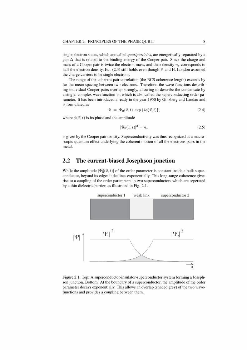
2.2 The current-biased Josephson junctionWhile the amplitude |Ψ2
0(~x, t)| of the order parameter is constant inside a bulk super-conductor, beyond its edges it declines exponentially. This long-range coherence givesrise to a coupling of the order parameters in two superconductors which are seperatedby a thin dielectric barrier, as illustrated in Fig. 2.1.
|Ψ | 2
1 2|Ψ |
2
x
superconductor 1 weak link superconductor 2
|Ψ|
Figure 2.1: Top: A superconductor-insulator-superconductor system forming a Joseph-son junction. Bottom: At the boundary of a superconductor, the amplitude of the orderparameter decays exponentially. This allows an overlap (shaded grey) of the two wave-functions and provides a coupling between them.
9 2.2. THE CURRENT-BIASED JOSEPHSON JUNCTION
2.2.1 Josephson equations
The theory describing a superconductor-insulator-superconductor system has been for-mulated by B. D. Josephson [37] in the year 1962. He predicted that a supercurrentwould tunnel through the insulating barrier even in the absence of voltage. Its magni-tude depends only on the phase difference ϕ = φ1 − φ2 between the order parametersof the two junction electrodes, also called the Josephson phase, and obeys the firstJosephson equation
I = Ic sin(ϕ), (2.6)
where Ic is the maximum (called critical) current which can flow without dissipation.Ic depends on the energy gap ∆ of the superconductor, the normal resistance of thetunnel barrier and the Cooper pair density. As long as the amplitude of a constantcurrent Ib flowing through the barrier does not exceed the critical current Ic , there isno voltage drop across the junction, and the Josephson phase according to Eq. (2.6)will be constant,
ϕ = arcsinIb
Ic+ 2πn. (2.7)
The second Josephson equation relates the time evolution of the phase difference ϕ tothe voltage V across the junction:
dϕ
dt=
2π
Φ0V =
2e
~V, (2.8)
where Φ0 = h/2e = 2.07 10−15 V s is the magnetic flux quantum, e is the electroncharge and h is Planck’s constant. Combining both equations implies that a constantvoltage applied to the junction results in an alternating current
I = Ic sin(
ϕ0 +2π
Φ0V t
), (2.9)
where the frequency-to-voltage ratio is given by
1Φ0
= 483.6MHzµV
. (2.10)
Vice versa, any change in the supercurrent and hence the Josephson phase will resultin a nonzero voltage. The junction thus acts like an ideal but nonlinear inductance. Bydifferentiating Eq. (2.6) and inserting Eq. (2.8), the Josephson inductance L can beobtained:
L = V
(dI
dt
)−1
=~2e
1Ic cos ϕ
. (2.11)
One should note that this inductance depends through the Josephson phase ϕ on thebias current through the junction and will also take negative values.
2.2.2 The RCSJ model
The dynamics of the Josephson phase can be understood in the frame of the resistivelyand capacitively shunted junction model (RSCJ model) introduced by Stewart [38] andMcCumber [39]. The model applies to small junctions, whose dimensions are smaller

CHAPTER 2. PRINCIPLES OF THE PHASE QUBIT 10
than the characteristic length λJ of spatial variations of the Josephson phase, typically5 to 30 µm. This length is calculated as [40]
λJ =
√Φ0
2πjc(2λL + t), (2.12)
where jc is the critical current density in A/cm2, λL the London penetration depth ofthe electrode material, t is the thickness of the insulating barrier and the electrodes areassumed to have a thickness larger than λL.
The junction is modeled by an equivalent circuit consisting of an ohmic resistor R,which represents its effective shunt resistance, a capacitor C accounting for the totalcapacitance of the junction electrodes and an element which behaves according to Eq.(2.6), see inset to Fig. 2.2.
XC R
Ib
0 2 4 6
15
10
5
0
U(ϕ
)
/
E
J −
−
−
π π πϕ
γ = 0.5
γ = 0.9
γ = 0
ω0
∆U
γ = 1.5
IN
ϕ ϕ0 m
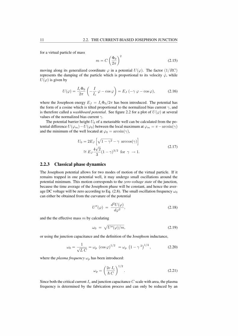
Figure 2.2: The washboard potential plotted for four different normalized bias currentsγ. The virtual particle is indicated by a solid disc. For γ = 0.5, the potential barrierheight ∆U is also shown. Inset: Equivalent circuit model of a Josephson junction.The Josephson supercurrent is symbolized by an X and the intrinsic capacitance andresistance are indicated as C and R, respectively. The fluctuation current source isconnected by dashed lines to the resistor.
According to Kirchhoff’s law, the total current flowing through such a system is thesum of the currents in each of the three paths. Using Eq. (2.9), this yields
I = Ic sin ϕ +V
R+ C
dV
dt= Ic sin ϕ +
1R
Φ0
2πϕ + C
Φ0
2πϕ. (2.13)
The right hand side of this equation can be written as an equation of motion,
mϕ + m1
RCϕ +
∂U(ϕ)∂ϕ
= 0, (2.14)
11 2.2. THE CURRENT-BIASED JOSEPHSON JUNCTION
for a virtual particle of mass
m = C
(Φ0
2π
)2
(2.15)
moving along its generalized coordinate ϕ in a potential U(ϕ). The factor (1/RC)represents the damping of the particle which is proportional to its velocity ϕ, whileU(ϕ) is given by
U(ϕ) =IcΦ0
2π
(− I
Icϕ− cos ϕ
)= EJ (−γ ϕ− cosϕ), (2.16)
where the Josephson energy EJ = IcΦ0/2π has been introduced. The potential hasthe form of a cosine which is tilted proportional to the normalized bias current γ, andis therefore called a washboard potential. See figure 2.2 for a plot of U(ϕ) at severalvalues of the normalized bias current γ.
The potential barrier height U0 of a metastable well can be calculated from the po-tential difference U(ϕm)−U(ϕ0) between the local maximum at ϕm = π−arcsin(γ)and the minimum of the well located at ϕ0 = arcsin(γ),
U0 = 2EJ
[√1− γ2 − γ arccos(γ)
]
∼= EJ4√
23
(1− γ)3/2 for γ → 1.
(2.17)
2.2.3 Classical phase dynamicsThe Josephson potential allows for two modes of motion of the virtual particle. If itremains trapped in one potential well, it may undergo small oscillations around thepotential minimum. This motion corresponds to the zero-voltage state of the junction,because the time average of the Josephson phase will be constant, and hence the aver-age DC voltage will be zero according to Eq. (2.8). The small oscillation frequency ω0
can either be obtained from the curvature of the potential
U ′′(ϕ) =d2U(ϕ)
dϕ2, (2.18)
and the the effective mass m by calculating
ω0 =√
U ′′(ϕ)/m, (2.19)
or using the junction capacitance and the definition of the Josephson inductance,
ω0 =1√L C
= ωp (cos ϕ)1/2 = ωp
(1− γ 2
)1/4, (2.20)
where the plasma frequency ωp has been introduced:
ωp =(
2e Ic
~ C
)1/2
. (2.21)
Since both the critical current Ic and junction capacitance C scale with area, the plasmafrequency is determined by the fabrication process and can only be reduced by an

CHAPTER 2. PRINCIPLES OF THE PHASE QUBIT 12
additional shunt capacitance to the junction. For typical tunnel junctions, νp = ωp/2πis in the microwave range with several tens of GHz.
If the particle once escaped from a well and the damping is not too high, i.e.(ωpRC)−1 ¿ 1, its kinetic energy will exceed the barrier height of the next well andthe particle continues to run down the washboard. The junction is then in its voltagestate: the phase increases steadily and a nonzero dc voltage appears according to thesecond Josephson equation (2.8). To retrap the particle in one well and hence to switchback to the zero-voltage state, it will be necessary to reduce the potential tilt substan-tially by reducing the applied bias current. This is the origin of the hysteresis observedon the current-voltage characteristics of a Josephson junction with low damping (seeFig. 2.3).
From the IV-curve, one can estimate the resistance of the barrier Rn when thejunction is in its normal state for currents larger than the critical current. The so-calledsubgap-resistance Rsg is given by the slope of the voltage dependence for currents justabove the retrapping current. The quasi-particle resistance at temperature T is thengiven by
Rqp = Rn exp(
∆kBT
), (2.22)
where kB = 1.38 · 10−23J/K denotes Boltzmann’s constant and the energy gap ∆is found from the measured gap voltage via ∆ = Vg e/2. This equation shows thatRqp should become extremely high at low temperatures, since the quasiparticle densityexponentially decreases with temperature as stated within the BCS theory.
Beneath a damping, the resistance provides another important contribution to thephase dynamics since every resistive element constitutes a source of current fluctua-tions at finite temperatures. This is indicated in Fig. 2.2 (a) as the additional currentsource IN which is connected with dashed lines to the resistor. The temporal aver-age of the noise current IN (t) at temperature T is given by the Johnson-Nyquist noiseformula and satisfies [41]
∫ ∞
−∞< IN (t)IN (0) >T eiωtdt = 2kBT/R. (2.23)
These fluctuations in the bias current result in variations of the position of the classicalparticle, which describes the state of the junction. This gives rise to a temperature-induced escape from the metastable well as discussed in chapter 2.2.5.
Quality Factor
A measure for the damping of the plasma oscillation by the effective shunt resistanceR of the junction is the dimensionless quality factor (Q factor). It relates the energyW stored in the oscillating system to the energy Wdiss dissipated during one cycle viaQ = ω0W/Wdiss. Thus, the Q factor estimates the number of periods during whichthe oscillation energy will be dissipated. When considering pure Ohmic damping, thequality factor of a Josephson junction is defined as
Q = RC ω0. (2.24)
High frequency contributions to dissipationAlthough the RSCJ model predicts many properties of the Josephson junction cor-
rectly and straightforward, one should be aware of the fact that the model is simplified

13 2.2. THE CURRENT-BIASED JOSEPHSON JUNCTION
0 1 2 3 44 3 2 1
Voltage V [ mV ]
100
300
500
700
100
300
500
700
Curr
ent
I[µ
A]
-
-
-
-
- - - -
Rn
gV
Ic
-Ic
Rsg
Figure 2.3: Current-voltage characteristic of a typical Josephson junction fabricatedfrom a Nb/Al/AlOx/Nb trilayer, measured at 20 mK temperature. Indicated by Ic isthe critical current and Vg denotes the gap voltage. The slope of the curve at highervoltages displays the normal resistance Rn w 5.2Ω of the barrier. Also indicated is thesubgap-resistance Rsg ≈ 400 Ω.
by assuming a frequency-independent shunt resistance which furthermore neglects anycontributions to the junction impedance at high frequencies arising from the bias cir-cuitry.
2.2.4 Macroscopic quantum effectsAt low temperatures and weak damping, the particle analog is no more suitable for anappropriate description of the phase dynamics because quantum effects become appar-ent. Experimentally, macroscopic quantum tunneling [2] and indications for energylevel quantization [42, 4] were found already 20 years ago.However, there should be a smooth transition between quantum and classical limits ofthe macroscopic system, and experimental results can often be interpreted in both pic-tures [43]. One example described in the following is the resonantly driven oscillator.This involves adding a small microwave (µW ) current component IµW of the form
IµW = Im sin(ωµW t + φµW ) (2.25)
to the bias current. Its frequency and amplitude are denoted as ωµW and Im, φµW is itsphase.
In the classical picture, the effects arising from the microwave current can be un-derstood as due to a periodic force driving the particle [44]. A maximum of energy istransferred to the particle when the frequency ωµW of the microwave is close to thenatural frequency of the oscillation in the well ω0.
For the same situation but in terms of the quantum picture, the photon energy ~ωµW
must be equal to the energy separation of the ground state and the first excited state toallow transitions between levels by the absorption or emission of one photon (see figure2.4).
The discrete energy levels in the quadratic potential well of a quantum mechanicalharmonic oscillator are located at (n+1/2) ~ω0, with n ≥ 0. The potential wells of the
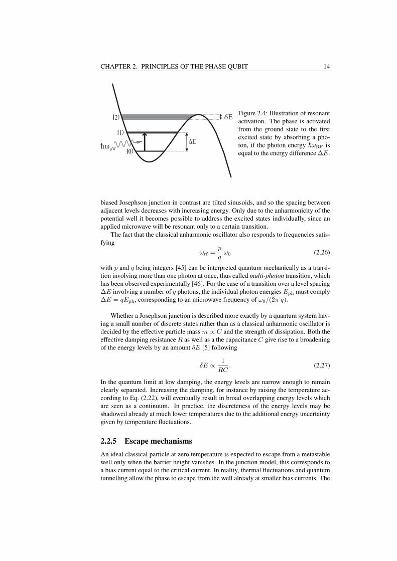
CHAPTER 2. PRINCIPLES OF THE PHASE QUBIT 14
1
0>
>
2>
µW
δEFigure 2.4: Illustration of resonantactivation. The phase is activatedfrom the ground state to the firstexcited state by absorbing a pho-ton, if the photon energy ~ωRF isequal to the energy difference ∆E.
biased Josephson junction in contrast are tilted sinusoids, and so the spacing betweenadjacent levels decreases with increasing energy. Only due to the anharmonicity of thepotential well it becomes possible to address the excited states individually, since anapplied microwave will be resonant only to a certain transition.
The fact that the classical anharmonic oscillator also responds to frequencies satis-fying
ωrf =p
qω0 (2.26)
with p and q being integers [45] can be interpreted quantum mechanically as a transi-tion involving more than one photon at once, thus called multi-photon transition, whichhas been observed experimentally [46]. For the case of a transition over a level spacing∆E involving a number of q photons, the individual photon energies Eph must comply∆E = qEph, corresponding to an microwave frequency of ω0/(2π q).
Whether a Josephson junction is described more exactly by a quantum system hav-ing a small number of discrete states rather than as a classical anharmonic oscillator isdecided by the effective particle mass m ∝ C and the strength of dissipation. Both theeffective damping resistance R as well as a the capacitance C give rise to a broadeningof the energy levels by an amount δE [5] following
δE ∝ 1RC
. (2.27)
In the quantum limit at low damping, the energy levels are narrow enough to remainclearly separated. Increasing the damping, for instance by raising the temperature ac-cording to Eq. (2.22), will eventually result in broad overlapping energy levels whichare seen as a continuum. In practice, the discreteness of the energy levels may beshadowed already at much lower temperatures due to the additional energy uncertaintygiven by temperature fluctuations.
2.2.5 Escape mechanismsAn ideal classical particle at zero temperature is expected to escape from a metastablewell only when the barrier height vanishes. In the junction model, this corresponds toa bias current equal to the critical current. In reality, thermal fluctuations and quantumtunnelling allow the phase to escape from the well already at smaller bias currents. The

15 2.2. THE CURRENT-BIASED JOSEPHSON JUNCTION
probability of escape may be expressed in terms of the lifetime τ of the zero-voltagestate, which is the inverse of the escape rate Γ
τ ≡ Γ−1. (2.28)
In the following, the two escape processes are discussed and formulas for the escaperate from the zero-voltage state are given for particular regimes.
Thermal activation
In the classical analog, the virtual particle can be regarded as being subject to Brownianmotion. The formula which describes the temperature dependence of the rate at whichthe particle can overcome the potential barrier of height U0 was found by Arrhenius. Itis given by the exponential negative ratio of the potential barrier height U0 (Eq. 2.17)to the thermal energy as the product of Boltzmann’s constant kB and temperature T .The rate of escape Γth due to thermal activation hence follows the equation
Γth = atω0
2πexp
(− U0
kBT
), (2.29)
where the pre-exponential factor ω02π resembles the attempt frequency towards the bar-
rier. Figure 2.5 illustrates the process of thermal activation.
ω0
U(ϕ)
Γth
U0
Figure 2.5: A zoom into onemetastable well where the analo-gous classical particle oscillates atfrequency ω0 around the potentialminimum. The brownian particleis pushed across the barrier heightU0 by thermal fluctuations in itsenergy at the thermal escape rateΓth.
Friction reduces the thermal excape rate nonexponentially as discussed in Kramer’sseminal paper [47] for the case of frequency independent (ohmic) damping. In themoderate to large damping regime, the escape is reduced due to back-diffusion over thebarrier top, while for very weak friction the highly excited states are depleted becauseof weaker influence of the heat bath to the system, which prevents it from being inthermal equilibrium. See [48] for a detailed review. These effects are taken into accountin the damping prefactor at, which can be approximated in the limit of low damping as[49]
at =4a
[(1 + Q kBT1.8U0
)1/2 + 1]2. 1, (2.30)
where a is a numerical constant close to unity.
Macroscopic quantum tunnelling
As the temperature approaches zero, the thermal escape rate is exponentially sup-pressed and the metastable state can only decay via macroscopic quantum tunnelling.

CHAPTER 2. PRINCIPLES OF THE PHASE QUBIT 16
The term macroscopic emphasizes the fact that this tunnelling concerns the Josephsonphase as a whole rather than single Cooper pairs.
The quantum tunnel rate Γqu may be calculated using the semi-classical Wentzel-
1>
2>
0 >
∆E hω0
Γ0
Γ1
∼ ∼
I II III
Figure 2.6: Quantum picture of the state of the Josephson phase inside the well,wherein the discrete energy levels are indicated as grey horizontal lines. Tunnellingfrom the excited state occurs at a rate Γ1, which is about 1000 times larger than thetunnel rate from the ground state Γ0 since the corresponding barrier height is reducedby the energy difference ∆E. Additionally shown is a sketch of the squared wavefunc-tions |Ψ|2 of the ground state |0〉 and the first excited state |1〉.
Kramers-Brillouin (WKB) approximation. In region I, the ground state wavefunctionΨI coincides with that of an anharmonic oscillator, whereas it declines exponentiallyin the classical forbidden region II, where E0 < U0(ϕ). The escape rate is then found[50] by relating the remaining probability |ΨIII|2 in region III to |ΨI|2, resulting in
Γqu =ω0
2π
(864π U0
~ω0
)1/2
exp(−36
5U0
~ω0
). (2.31)
The effect of damping on quantum tunnelling was investigated in the work of Caldeiraand Leggett [51, 52] by modelling the friction as a coupling to an infinite set of har-monic oscillators. The tunnel rate is then expressed as
Γqu = A exp(−B) (2.32)
with
A =√
60 ω0
(B
2π
)1/2
(1 +O(Q−1)),
B =365
U0
~ω0(1 +
1.74Q
+ O(Q−2)),
(2.33)
where the WKB-result is recovered for Q À 1. Note that damping affects the quantumtunnel rate exponentially, in contrast to the thermal activation rate.
Tunnelling from excited states happens at an exponentially higher rate, since the

17 2.3. COHERENT DYNAMICS IN THE TWO-STATE SYSTEM
corresponding barrier height is reduced by the energy of the excited level. For typicalbias currents where tunnelling becomes observable (γ & 0.99), the escape rate fromthe first excited state is three orders of magnitude higher than the one from the groundstate. This allows to deduce the quantum state of the phase before it tunnelled bymeasurements of the lifetime of the zero-voltage state.
Cross-over regime
The transition from the dominance of thermal activation to macroscopic tunnellinghappens around the cross-over temperature T ∗, for which an estimation is [48]
T ∗ ' ~ω0
2πkB
[(1 +
12Q
2)1/2
− 12Q
]. (2.34)
The Q-dependent damping factor in this equation decreases the cross-over temperatureby less than 1% for junctions with Q > 50.
Quantum corrections have to be applied to the thermal activation rate already abovethe cross-over temperature, since the tunnelling from thermally excited states is expo-nentially increased due to the smallness of the remaining barrier. Indications for theexistence of quantized energy levels above the crossover temperature were found exper-imentally by Silvestrini et. al. [53]. At finite temperature and in thermal equilibrium,the occupation probability ρn for the n−th level is given by the Boltzmann distribution[54]
ρn = Ξ−1 exp (−En/kBT ) , Ξ =∞∑
n=0
exp (−En/kBT ) . (2.35)
The total escape rate is then the sum of the rates from each individual level multi-plied by its occupation probability. A useful approximation to the escape rate in theintermediate temperature regime 1.4 T ∗ . T . 3T ∗ is [55]
ΓT∗ = aiω0
2πexp
(− U0
kBT
)(2.36)
where the prefactor ai valid to first order in 1/Q is
ai =sinh(~ω0/2kBT )sin(~ω0/2kBT )
. (2.37)
Equation (2.36) assumes the population in the excited levels to strictly obey the Boltz-mann distribution. At higher temperatures, the escape rate is therefore correctly givenonly by Eq. (2.29), where the depletion of excited states through tunnelling is consid-ered in the thermal prefactor at.
2.3 Coherent dynamics in the two-state systemThe theoretical treatment of two-level quantum systems is of fundamental importancefor the description of a great variety of quantum effects. A well-studied example isthe spin-1/2 particle in an external magnetic field which constitutes an analogon toany two-state system, and hence quantum bits also fall into this categorie. The samemathematical apparatus can be used to describe a current-biased Josephson junction if

CHAPTER 2. PRINCIPLES OF THE PHASE QUBIT 18
its energy spectrum can be truncated to the lowest to levels. In this case, an externalperturbation is realized by an applied microwave current at close resonance, i.e. its fre-quency ωrf is practically equal to the small oscillation frequency ω10 given by Equation(2.20).
The effect of such a perturbation or coupling is two-fold. Statically, it results in achange of the position of the energy levels. Dynamically, coherent oscillations betweenthe two states appear, which are of particular experimental interest for the creation ofstate superpositions.
2.3.1 Rabi oscillationRabi oscillations are coherent oscillations between the eigenstates of a two-level quan-tum system which is subject to a resonant perturbation. The calculation of the Rabifrequency and amplitude poses a standard problem which is discussed in many bookson quantum mechanics. Here, I follow the notation of [56]. The result is then beapplied to the current-biased Josephson junction.
A two-level system without any perturbation is described by its Hamiltonian H0.By using its eigenstates |ϕ0〉 and |ϕ1〉 as a basis, the stationary Schrodinger equationreads
H0 |ϕ0〉 = E0 |ϕ0〉H0 |ϕ1〉 = E1 |ϕ1〉 ,
(2.38)
where E0 and E1 are the corresponding eigenenergies and the Hamiltonian has thediagonal form
H0 =(
E0 00 E1
). (2.39)
When the perturbation is switched on, the new Hamiltonian becomes
H = H0 +W, (2.40)
where W denotes the perturbation or coupling operator. As a result, we expect bothnew eigenstates, denoted |Ψ+〉 and |Ψ−〉, and new eigenenergies E+ and E−. Equation(2.38) then becomes
H |Ψ+〉 = E+ |Ψ+〉H |Ψ−〉 = E− |Ψ−〉 .
(2.41)
The coupling is represented by the hermitian matrix
W =(
W00 W01
W10 W11
)(2.42)
with W00 as well as W11 being real and W01 = W ∗10. We can assume that both W00
and W11 are equal to zero since their effect can be implicitly taken into account byreplacing E0 and E1 in equation (2.39) by E′
0 = E0 + W00 and E′1 = E1 + W11,
respectively. For the diagonalization of the new hamiltonian (2.40) we shall follow theprocedure given in [56], which yields the two eigenvalues
E± =12(E0 + E1)± 1
2
√(E0 − E1)2 + 4|W01|2 (2.43)
19 2.3. COHERENT DYNAMICS IN THE TWO-STATE SYSTEM
and the two eigenvectors
|Ψ+〉 = cos(
θ
2
)e−iϕ/2 |ϕ0〉+ sin
(θ
2
)eiϕ/2 |ϕ1〉
|Ψ−〉 = − sin(
θ
2
)e−iϕ/2 |ϕ0〉+ cos
(θ
2
)eiϕ/2 |ϕ1〉 .
(2.44)
The angels θ and ϕ refer to those used in the Bloch-sphere description of section 2.3.3,and are defined as
tan θ =2|W01|
E0 − E1, 0 ≤ θ < π,
W10 = eiϕ |W10|.(2.45)
Since the time evolution of the quantum state follows the Schrodinger equation
i~ddt
|Ψ(t)〉 = H |Ψ(t)〉 , (2.46)
we can write|Ψ(t)〉 = α e−i E+t/~ |Ψ+〉+ β e−i E−t/~ |Ψ−〉 . (2.47)
α and β are determined by the initial condition, for which we define the system to bein the ground state |Ψ(0)〉 = |ϕ0〉 at time t = 0. We can now rewrite Eq. (2.47) bysolving Eq. (2.44) for |ϕ0〉,
|Ψ(0)〉 = |ϕ0〉 = eiϕ/2 [cos(
θ
2
)|Ψ+〉 − sin
(θ
2
)|Ψ−〉] (2.48)
and we obtain
|Ψ(t)〉 = eiϕ/2 [ e−i E+t/~ cos(
θ
2
)|Ψ+〉 − e−i E−t/~ sin
(θ
2
)|Ψ−〉]. (2.49)
To show that the state (2.49) indeed oscillates between the unperturbed states |ϕ0〉 and|ϕ1〉, we first write
〈ϕ1|Ψ(t)〉 = eiϕ/2 sin(
θ
2
)cos
(θ
2
)[ e−i E+t/~ − e−i E−t/~] (2.50)
and use this to calculate the probability P1(t) = |〈ϕ1|Ψ(t)〉|2 to find the system instate |ϕ1〉 at time t: 1
P1(t) =12
sin2 θ
[1− cos
(E+ − E−
~t
)]
= sin2 θ sin2
(E+ − E−
2~t
),
(2.51)
which after substitution of (2.43) and (2.45) reads
P1(t) =4|W01|2
4|W01|2 + (E0 − E1)2sin2
[√4|W01|2 + (E0 − E1)2
t
2~
](2.52)
1By making use of the identity sin2(θ/2) cos2(θ/2) = 14
sin2(θ) and Euler’s formula we find
| e−i E+t/~ − e−i E−t/~ |2 = 2[1− cos(E+−E−
~ t)].
CHAPTER 2. PRINCIPLES OF THE PHASE QUBIT 20
Known as Rabi’s formula, equation (2.52) describes a sinusoidal oscillation of P1 atthe so-called Rabi-frequency
ωR =√
4|W01|2 + (E0 − E1)212~
(2.53)
and with an amplitude which is close to one if the coupling is strong, or |W01| À|E0 − E1|.
Decoherence effects
As it was mentioned before, the discrete phase eigenstates of a Josephson junction arenot stable. For example, the ground state can decay by tunnelling at the rate Γ0 towardsthe continuum, and the excited state can additionally fall back to the ground state dueto dissipation at the rate Γd. Furthermore, the coherence of the superposition state isaffected by dephasing at the rate Γφ.
To show how this influences the time-dependent level population as calculated inequation (2.52), we can define the total off-diagonal decay rate Γ as the sum of indi-vidual decoherence rates [57], i.e. Γ = Γ0 + Γ1 + Γd + 2Γφ. Quantum mechanicsallows to phenomenologically take into account the finite lifetime of a state by addingan imaginary term to its energy, which is then given by2
E′n = En − i ~
Γ2
. (2.54)
Following the calculation in section 2.3.1, we note that the time-evolution operator willbe replaced by
e−i E′nt/~ = e−i En t/~ · e−Γ2 t/~. (2.55)
For the time-dependent population of the excited level we obtain
P1(t) =|W01|2
|W01|2 −(~
2Γ)2 e−Γt sin2
√|W01|2 −
(~2
Γ)2
t
2~
. (2.56)
Equation (2.56) is valid for |W01| > ~2Γ. This means that the excited level population
will undergo damped sinusoidal oscillations if the coupling is strong enough to suffi-ciently increase the Rabi frequency so that the system can oscillate before it becomesincoherent, see Fig. 2.7.
Detuning
The externally applied microwave frequency might not be tuned exactly to the transi-tion frequency and differ by a value of
∆ =|E1 − E0|
~− ωrf . (2.57)
Any detuning ∆ results in a higher oscillation frequency and decreases the amplitude.The oscillating population probability of the excited level corrected for detuning is
P1(t) =|W01|2
|W01|2 + ∆2sin2
[√|W01|2 + ∆2
t
2~
]. (2.58)
Figure 2.8 shows that for larger detuning the amplitude decreases, while the Rabi fre-quency increases.
2see [56], complement HIV.

21 2.3. COHERENT DYNAMICS IN THE TWO-STATE SYSTEM
2 4 6 8 10 12
0.2
0.4
0.6
0.8
P1
t
Figure 2.7: A plot of equation(2.56) for a low decoherence rate(~
2Γ)
= 0.1|W01| shows exponen-tially decaying oscillations. For alarge decoherence rate,
(~2Γ
)=
1.5|W01|, oscillations do not oc-cur.
1 2 3 4 5 6
0.2
0.4
0.6
0.8
1P1
t
Figure 2.8: The excited level pop-ulation P1(t) as given by equa-tion (2.58), plotted for the detun-ings ∆ = 0, 2|W01| and 4|W01|,respectively.
Mapping to the case of the Josephson junction
For the microwave-irradiated Josephson junction, we can write its bias current as I(t) =I + Idc(t) + ∆Irf(t), which is the sum of the constant I , a component Idc(t) vary-ing slowly compared to the small oscillation frequency and the microwave component∆Irf(t) = Irf [cos (ωrf t)+i sin (ωrf t)]. Irf is the absolute amplitude of the alternatingcurrent. Slow variations of Idc will result in a change of the energy scale of the systemand hence affect only the diagonal components of the Hamiltonian. Its non-diagonal(coupling) matrix element can be reduced to be proportional just to the microwaveamplitude by applying the rotating wave approximation and is then given by [58]
W01 = 〈0|φ |1〉 Φ0
2πIrf . (2.59)
If we assume that the potential is sufficiently harmonic for U(φ) . E1, the overlapmatrix element of the harmonic oscillator can be used, which is
〈0|ϕ |1〉 =√
~2 mω0
=2π
Φ0
√~
2 ω0 C, (2.60)
where the effective mass of the virtual particle (2.15) has been inserted for m. We findthe Rabi frequency from equation (2.53), which reduces to
ωR =|W01|~
(2.61)
for the case of strong coupling and low damping (|W01| À |E0 − E1| À |~Γ/2|)and a resonant (ωrf = ω01) stimulation. The strong coupling condition is preferred

CHAPTER 2. PRINCIPLES OF THE PHASE QUBIT 22
in experiments in order to obtain both large frequency and amplitude of the coherentoscillation, which will then be less affected by detuning and decoherence. Finally, weobtain
ωR =Irf
~
√~
2ω0 C= η |〈0|ϕ |1〉| EJ
~(2.62)
where we have defined η = Irf/Ic as the microwave amplitude normalized to thecritical current and we make use of the Josephson energy EJ = IcΦ0/(2π).
2.3.2 Energy-level repulsion
To discuss the modifications of the energy levels due to the coupling, we rewrite equa-tion (2.43) for the energy eigenvalues:
E+ = Em +√
E∆2 + |W01|2
E− = Em −√
E∆2 + |W01|2,
(2.63)
Em =12(E0 + E1)
E∆ =12(E0 − E1)
(2.64)
where E0 and E1 are still the energies of the unperturbed states. For conditions wherethese are equal (E∆ = 0), the most striking feature is that the coupling separates themby the amount of 2|W01|. Figure 2.9 shows a plot of the eigenenergies. The asymptotesto the eigenenergies for large E∆ are the unperturbed energies E0 and E1. This anti-crossing of the energy levels has been observed in the tunable double-well potentialof a SQUID [7, 59] and was the first experimental proof of coherence for the phasevariable in a Josephson junction incorporated into a superconducting loop.
E+
E-
E0
E1
|W |01
-|W |01
E∆
Energies
Figure 2.9: A plot of the eigenenergies of the states without coupling (E0 and E1)and with non-diagonal coupling (E+ and E−) versus their energy difference E∆ =(E0 − E1)/2.
In the case where the levels are separated but the coupling is weak (E∆ À |W01|,

23 2.3. COHERENT DYNAMICS IN THE TWO-STATE SYSTEM
equation (2.63) can be approximated as
E± = Em ± E∆
(1 +
12
∣∣∣∣W01
E∆
∣∣∣∣2
+ . . .
), (2.65)
showing that the effect on the energies is of second order in the coupling strength. Incontrast, for strong coupling or E∆ ¿ |W01|, we obtain
E± = Em ± |W01| (2.66)
which results in a more significant change of the eigenenergies since it is an effect offirst-order in |W01|.
2.3.3 Bloch-sphere description of the qubit stateThe state of the quantum bit can be represented by a vector |Ψ〉 contained in the Hilbertspace which is spanned in the computational basis by the two logical states |0〉 and |1〉,
|Ψ〉 = a |0〉+ b |1〉 , (2.67)
where the square of the amplitudes |a|2 and |b|2 correspond to the probability to findthe qubit in state |0〉 or |1〉, respectively. Accordingly, these probabilities must sumto one, leading to the normalization condition 〈Ψ|Ψ〉 = |a|2 + |b|2 = 1. While ingeneral a and b are complex numbers, it is only the absolute value of the coefficientswhich is observable by a measurement of the qubit state, and therefore only the phasedifference between the coefficients remains to be considered. Together with the nor-malization condition, the four dimensional configuration space therefore reduces to atwo dimensional subspace [60, 19].
It is instructive to illustrate the quantum state of a single qubit within the Blochvector picture. If the qubit remains in a pure state, that is, |a|2 + |b|2 = 1, then theBloch vector points to the surface of a unit sphere as shown in Fig. 2.10. The qubitstate is determined by the polar and azimuthal angels φ and θ according to
|Ψ〉 = cos (θ/2) |0〉+ ei φ sin (θ/2) |1〉 . (2.68)
The squared projection of the state vector to the ~z-axis, which is assumed to be thequantization axis, gives the occupation probability of the two logical states, which forthe ground state reads p0 = cos2(θ/2). The precession around the ~z-axis at the Lar-mor frequency ω10 arising from the energy difference between the two states is takeninto account conveniently by changing to the ω10-rotating frame. This implies that thephase φ does not change as long as all external parameters remain constant.
Logical operations on qubits are also called quantum gates and correspond to trans-formations of the state vector which must be unitary (and hence reversible) to ensurethat a pure state gets mapped to a pure state. In the Bloch picture, these single-qubitoperations correspond to rotations around the three axis ~x, ~y and ~z. A unitary rota-tion operator R~n(α) defining a rotation around the unit vector ~n by an angle α can bewritten with the use of the set of Pauli spin operators σ = σx, σy, σz and reads
R~n(α) = exp(−i
α
2~n · σ
)(2.69)
= I cos(α/2)− i sin(α/2) ~n · σ, (2.70)

CHAPTER 2. PRINCIPLES OF THE PHASE QUBIT 24
where I denotes the unity operator. For example, the qubit is transferred from theground state |0〉 to the superposition state (|0〉+ |1〉) /
√2 by rotating the Bloch vector
around the ~y-axis by an angle of π/2 with the matrix operator
R~y(π/2) =(
cos (π/2) − sin (π/2)sin (π/2) cos (π/2)
)=
1√2
(1 −11 1
). (2.71)
This operation is therefore referred to as a ”π/2-pulse” in literature and has the sameeffect as the Hadamard transformation3. Experimentally, rotating the Bloch vectoraround the x− or y−axis is possible via the discussed mechanism of Rabi oscillationby applying a resonant perturbation. Another important single-qubit operation is theNOT -gate which is defined by NOT |0〉 = |1〉 and NOT |1〉 = |0〉. It is obviouslyrealized by rotating the Bloch vector around θ = 180o by applying a π-pulse.
2.3.4 DecoherenceIn the discussed approach of using the phase eigenstates of a superconducting tunneljunction as a quantum bit, the two logical states are of different energies. This impliesthat energy has to be interchanged with the environment to modify the angle θ. It hasbeen discussed in the previous chapters that this is possible either by dissipating energy
3In quantum information theory, for the Hadamard transformation one uses the idempotent matrix1√2
(1 11 −1
)rather than (2.71).
z
φ
θ
y
x
1>
0>
Figure 2.10: Bloch-sphere representation of the qubit state. The ground state |0〉 isrepresented by a vector pointing to the north pole , the state |1〉 corresponds to a vectorpointing to the south pole and all equally weighted superpositions are found along theequator for θ = π/2.
25 2.3. COHERENT DYNAMICS IN THE TWO-STATE SYSTEM
or by an alternating bias current component near the transition frequency between thelevels. The Josephson junction is coupled to the enviroment mainly by the necessarybiasing wires. Noise currents flowing in these lines at frequencies close to the transitionfrequency ω10 will therefore alter the occupation probabilities of the two levels byprocesses similar to stimulated absorption and emission. It has been shown in [58]that the probability p to measure the initially prepared state |0〉 or |1〉 would decayexponentially in time to p → 0.5 if dissipation would be neglected, because noise-induced emission as well as absorption occurs at an equal rate. In fact, dissipationplays a major role and gives rise to the relaxation of an excited state to the ground statefollowing an exponential decay law with the mean lifetime Γd
−1 as defined in equation(3.4).
Fluctuating currents at low frequencies result in changes of the transition frequencyaccording to Eq. (2.20). This has the effect that the state vector drifts from the rotatingframe, giving rise to a change of the phase φ of the Bloch vector. The probability thata given state is not altered by dephasing decreases exponentially in time, and so it ispossible to define the dephasing rate Γφ. Although fluctuations in the phase φ do notchange the level population directly, they may alter the outcome of subsequent qubitoperations, because the result of any rotation around one of the three axis dependson the direction of the Bloch vector. It is, for instance, obvious from Fig. 2.10 thatfor θ = 0 or θ = π the quantum state is not altered by rotations around ~z, i.e. theground and the excited state will not be sensitive to low frequency noise. In turn, thesuperposition state of the quantum bit is subject to modifications by current fluctuationseven without the need to interchange energy with the environment.

CHAPTER 2. PRINCIPLES OF THE PHASE QUBIT 26

Chapter 3
The flux-biased phase qubit
In this chapter, it will be discussed that the fidelity of directly current-biased phasequbits suffers from two major decoherence sources: the strong coupling to the electricalenvironment as given by the electrical wires connecting the junction, and the presenceof quasiparticles which are created in the readout process during which a switching tothe resistive state occurs. Both these problems are overcome when the junction biascurrent is sent through a superconducting transformer, hereby enclosing the junctionin a superconducting loop and thus creating an rf-SQUID. After a brief review of therf-SQUID principles, the technique to operate it as a phase qubit will be explained.The required ingredients for qubit bias and readout are discussed from the viewpointof the experimentalist, arriving at a presentation of the sample layouts and a discussionof relevant parts of the measurement apparatus.
3.1 Qubit isolation
3.1.1 Dissipation in the environment
As it has been discussed in the preceding chapter, the two logical states of the phasequbit are Josephson phase eigenstates of different energies. Dissipation of energy there-fore causes relaxation of the excited state towards the stable ground state of lower en-ergy, limiting the qubit coherence time T1.
One source of dissipation is the intrinsic subgap resistance Rsg of the junction di-electric, which has been introduced within the frame of the RCSJ model discussed insection 2.2.2. As it has been shown in Ref. [61], this resistance can be optimized byan epitaxial growth of the junction base electrode, hereby creating an atomically flatsurface which after subsequent oxidation results in a smooth dielectric film. However,in a directly current-biased junction, the dominant source of dissipation occurs in theelectrical environment. Any circuit connected to the junction will provide a compleximpedance Ze(ω) to the Josephson element which is defined as the ratio of the com-plex amplitudes of the voltage response of the environment to the current oscillatingat frequency ω. The dissipative contributions from the external impedance Ze(ω) arecontained in its real part Re(ω) = Re[Ze(ω)]. The effective junction resistance arisingfrom the parallel shunt impedance is calculated from 1/Reff(ω) = 1/Rsg + 1/Re(ω).This expression shows that an external impedance Ze which is large compared to theimpedance of the junction ZJ will reduce dissipation to the amount determined by the
27

CHAPTER 3. THE FLUX-BIASED PHASE QUBIT 28
subgap resistance. By defining the reactive part of the junction impedance as [62]
ZJ =
√L
C=
1ω0C
, (3.1)
hereby using the inductance L defined in Eq. (2.20), the junction remains isolated fromthe environment response as long as |Ze(ω0)| À ZJ(ω0) at the frequency of the plasmaoscillations ω0. Because typical junction impedances of the order of ten ohms are com-parable to these of biasing wires and on-chip transmission lines (∼ 100Ω), a significantportion of loss may occur in these lines, resulting in enhanced damping and fast relax-ation.
3.1.2 Relaxation rateThe life time of the excited state T1 is proportional to the effective resistance Reff . Thedecay rate from the excited state to the ground state Γ01 ≡ 1/T1 can be calculated from[57]
Γd =2π(E1 − E0)
~RQ
Reff|〈0| ϕ
2π|1〉|2
[1 + coth
(E1 − E0
2kBT
)](3.2)
with E1 − E0 being the energy separation between the states |1〉 and |0〉 and Rq =h/4e2 being the resistance quantum. In the limit of low temperatures kBT ¿ E1, byusing the harmonic oscillator matrix element [58]
〈0|ϕ |1〉 = (2π/Φ0)√~/2ω10C, (3.3)
one obtainsΓd = 1/ ReffC. (3.4)
For a typical junction capacitance C of order 1 pF and an effective wire resistanceReff ∼ 100Ω, the life time T1 ≡ Γ−1
d according to Eq. (3.4) is less than 1 ns, empha-sizing the cruciality of special means to isolate the qubit junction from a low impedanceenvironment.
3.1.3 Inductive isolationTo avoid energy relaxation, the electrodynamic environment of the junction must becarefully designed. One possibility is to isolate the qubit junction by means of aninductive isolation network [63], which can be realized from on-chip capacitors andsuperconducting inductors. The output impedance of a parallel LC-resonant filter atworking frequencies beyond its resonance frequency of 1/
√LC grows with its induc-
tance L. Effective isolation therefore demands high values of both inductance and ca-pacitance which accordingly consume large space on chip. By exploiting the Josephsoninductance of an additional junction which is connected in parallel to the smaller qubitjunction [10], the circuit can be kept small and the amount of isolation can furthermorebe adjusted in situ [64]. A disadvantage of this approach, beneath the additional sub-gap resistance of the isolating junction, is that the qubit junction is still switching to aresistive state during the readout process. In the non-zero voltage state, the potentialdifference across the junction gives rise to generation of quasiparticles, which will per-sist for some time after the junction is reset to the superconducting state. These quasi-particles remain a source of decoherence because they provide normal current channelseffectively shunting the qubit and give rise to shot-noise and charge fluctuations [65].
29 3.1. QUBIT ISOLATION
Above mentioned problems are avoided when the qubit junction is isolated fromthe bias circuitry by means of a superconducting transformer [27]. We adopted thisapproach in our experiments on phase qubits.
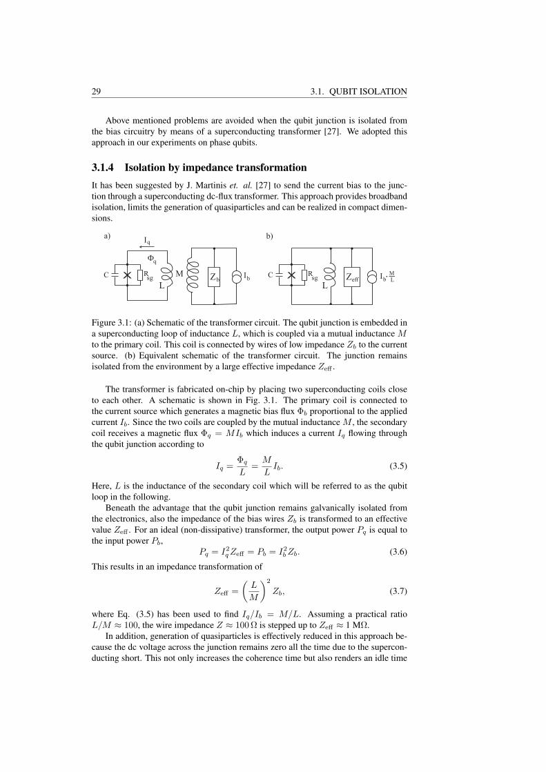
3.1.4 Isolation by impedance transformationIt has been suggested by J. Martinis et. al. [27] to send the current bias to the junc-tion through a superconducting dc-flux transformer. This approach provides broadbandisolation, limits the generation of quasiparticles and can be realized in compact dimen-sions.
L
M Z IbXC
a) b)
bRsg
LZ Ibeff
ML
Iq
Φq
XC Rsg
Figure 3.1: (a) Schematic of the transformer circuit. The qubit junction is embedded ina superconducting loop of inductance L, which is coupled via a mutual inductance Mto the primary coil. This coil is connected by wires of low impedance Zb to the currentsource. (b) Equivalent schematic of the transformer circuit. The junction remainsisolated from the environment by a large effective impedance Zeff .
The transformer is fabricated on-chip by placing two superconducting coils closeto each other. A schematic is shown in Fig. 3.1. The primary coil is connected tothe current source which generates a magnetic bias flux Φb proportional to the appliedcurrent Ib. Since the two coils are coupled by the mutual inductance M , the secondarycoil receives a magnetic flux Φq = MIb which induces a current Iq flowing throughthe qubit junction according to
Iq =Φq
L=
M
LIb. (3.5)
Here, L is the inductance of the secondary coil which will be referred to as the qubitloop in the following.
Beneath the advantage that the qubit junction remains galvanically isolated fromthe electronics, also the impedance of the bias wires Zb is transformed to an effectivevalue Zeff . For an ideal (non-dissipative) transformer, the output power Pq is equal tothe input power Pb,
Pq = I2q Zeff = Pb = I2
b Zb. (3.6)
This results in an impedance transformation of
Zeff =(
L
M
)2
Zb, (3.7)
where Eq. (3.5) has been used to find Iq/Ib = M/L. Assuming a practical ratioL/M ≈ 100, the wire impedance Z ≈ 100Ω is stepped up to Zeff ≈ 1 MΩ.
In addition, generation of quasiparticles is effectively reduced in this approach be-cause the dc voltage across the junction remains zero all the time due to the supercon-ducting short. This not only increases the coherence time but also renders an idle time

CHAPTER 3. THE FLUX-BIASED PHASE QUBIT 30
after each measurement unnecessary, which is otherwise essential to allow unpairedelectrons to recondense into Cooper pairs.
3.2 rf-SQUID principlesBy embedding the junction in the superconducting loop, the circuit becomes an rf-SQUID [8, 9]. In this section, the principles of the rf-SQUID are reviewed.
3.2.1 Potential energyFlux quantization links the total flux Φq in the rf-SQUID loop to the phase drop ϕacross the junction [8],
ϕ +2πΦq
Φ0= 2πn, (3.8)
where n is an integer. From this equation, the phase-flux relation
ϕ = −2πΦq
Φ0, (3.9)
is deduced for n = 0. The Josephson phase ϕ is in turn related by the first Josephsonequation (2.6) to the supercurrent flowing in the loop, which using Eq. (3.9) reads
Iq = −Ic sin(2πΦq/Φ0). (3.10)
Due to the loop inductance L, this current Iq generates a magnetic flux which adds upto an externally applied flux Φext. The resulting total flux threading the qubit loop Φq
is thereforeΦq = Φext + LIq = Φext − LIc sin(2πΦq/Φ0). (3.11)
In Figure 3.2, Φq given by Eq. (3.11) is plotted for different values of the parameterβL ≡ 2πLIc/Φ0. For βL > 1, the flux in the loop Φq is multivalued in some regionsof the external flux Φext, which causes Φq to switch in a hysteretic manner betweenflux states when the external magnetic flux is varied. This behavior was first observedexperimentally in the year 1967 by Silver and Zimmermann [66]. The plot of the loopcurrent versus the external flux shown in Fig. 3.2 (b) reveals that the switching betweenflux states is related to a reversal of the circulation direction of the loop current, whileits amplitude is always smaller than the critical current of the junction.
The potential energy of the rf-SQUID is the sum of the junction energy given inEq. (2.16) and the magnetic energy LI2
q /2 which is stored in the loop inductance L.Rewriting Eq. (3.11) to obtain the circulating current in the form Iq = (Φq −Φext)/L,we arrive at the rf-SQUID potential
U(ϕ) = EJ
[1− cos ϕ +
(ϕ− 2πΦext/Φ0)2
2βL
], (3.12)
using the Josephson energy EJ = ~IC/2e. This potential has the form of a parabolacentered at ϕ0 = 2πΦext/Φ0 and modulated by a cosine. As it is shown in Fig. 3.3,for larges values of βL the potential has many minima, while for βL < 1 only a singleminimum exists. Each minimum corresponds to a certain number of flux quanta in theloop, and accordingly, the mentioned switching between flux states is associated witha transition between the wells.

31 3.2. RF-SQUID PRINCIPLES
0
0.5
1
1.5
2
0 0.5 1 1.5 2
0
0.5
Φext
/ Φ0
β = 3l
Φq
/Φ
0
-0.5
0.80.1
I q/
Φ0
β = 3l
0.8
0.1
(a)
(b)
Figure 3.2: (a) Total magnetic flux in the qubit loop Φq/Φ0 versus the externally ap-plied flux Φext/Φ0 for different values of the parameter βL. The switching betweenflux states is indicated by arrows. (b) Dependence of the current Iq/Ic circulating inthe loop on the externally applied flux Φext/Φ0 for different values of the parameterβL.
Aiming at operating the rf-SQUID as a phase qubit, for a given junction criticalcurrent the loop inductance is designed such that 1 < βL < 4.6. This results in apotential that has not more than two minima for all values of externally applied fluxand one single minimum for Φext ≈ 0. If βL is larger than 4.6, it is still possible tooperate the rf-SQUID as a phase qubit, but in this case more than one minima exist inthe potential at all values of external flux, and therefore it becomes more difficult toinitialize the flux state of the qubit in a certain well.
By changing the external magnetic flux Φext, the double well potential appearsto be tilted as plotted in Fig. 3.4 (a). This allows to adjust the depth of the potentialwells in situ. Analogously to the critical current Ic of a biased Josephson junction,for the rf-SQUID there exists a critical flux Φc where the potential barrier between theshallow and the deep well vanishes. Its value can be found from the condition thatthe inflection point of the potential coincides with the position of the minimum of the
CHAPTER 3. THE FLUX-BIASED PHASE QUBIT 32
−2 −1 0 1 2 3
0
5
10
15
Phase difference ϕ
U /
EJ
β = 0.8l
β = 3l
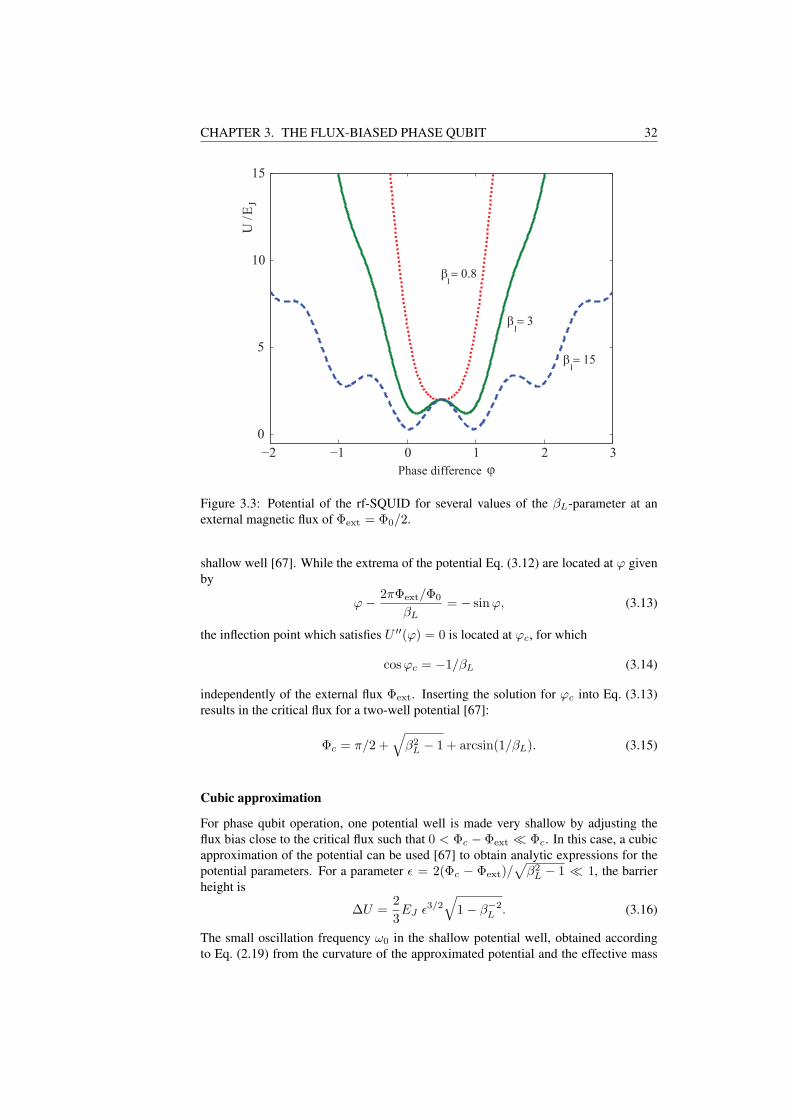
β = 15l
Figure 3.3: Potential of the rf-SQUID for several values of the βL-parameter at anexternal magnetic flux of Φext = Φ0/2.
shallow well [67]. While the extrema of the potential Eq. (3.12) are located at ϕ givenby
ϕ− 2πΦext/Φ0
βL= − sin ϕ, (3.13)
the inflection point which satisfies U ′′(ϕ) = 0 is located at ϕc, for which
cosϕc = −1/βL (3.14)
independently of the external flux Φext. Inserting the solution for ϕc into Eq. (3.13)results in the critical flux for a two-well potential [67]:
Φc = π/2 +√
β2L − 1 + arcsin(1/βL). (3.15)
Cubic approximation
For phase qubit operation, one potential well is made very shallow by adjusting theflux bias close to the critical flux such that 0 < Φc − Φext ¿ Φc. In this case, a cubicapproximation of the potential can be used [67] to obtain analytic expressions for thepotential parameters. For a parameter ε = 2(Φc − Φext)/
√β2
L − 1 ¿ 1, the barrierheight is
∆U =23EJ ε3/2
√1− β−2
L . (3.16)
The small oscillation frequency ω0 in the shallow potential well, obtained accordingto Eq. (2.19) from the curvature of the approximated potential and the effective mass
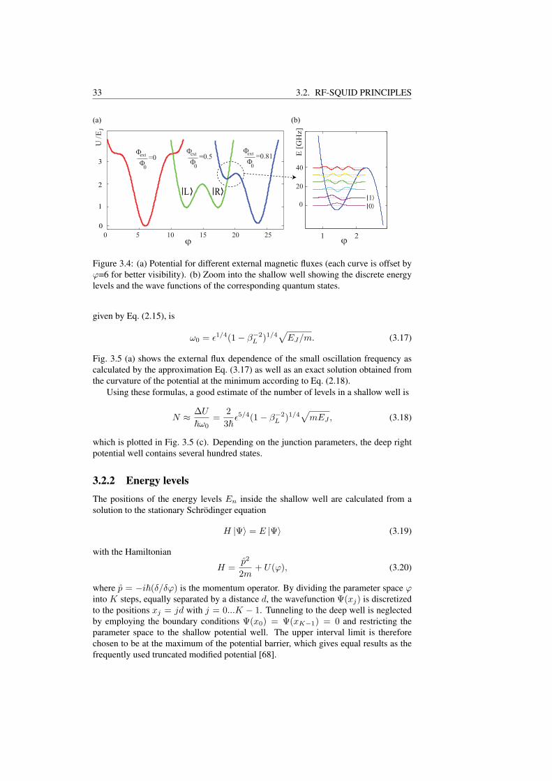
33 3.2. RF-SQUID PRINCIPLES
0 5 10 15 20 25
Φext=0
Φ0
R >L >
ϕ
Φext=0.5
Φ0
Φext=0.81
Φ0
3
1
0
2
1 2
0
20
40
ϕ
E [
GH
z]
U /
EJ
(a) (b)
0>
1>
Figure 3.4: (a) Potential for different external magnetic fluxes (each curve is offset byϕ=6 for better visibility). (b) Zoom into the shallow well showing the discrete energylevels and the wave functions of the corresponding quantum states.
given by Eq. (2.15), is
ω0 = ε1/4(1− β−2L )1/4
√EJ/m. (3.17)
Fig. 3.5 (a) shows the external flux dependence of the small oscillation frequency ascalculated by the approximation Eq. (3.17) as well as an exact solution obtained fromthe curvature of the potential at the minimum according to Eq. (2.18).
Using these formulas, a good estimate of the number of levels in a shallow well is
N ≈ ∆U
~ω0=
23~
ε5/4(1− β−2L )1/4
√mEJ , (3.18)
which is plotted in Fig. 3.5 (c). Depending on the junction parameters, the deep rightpotential well contains several hundred states.
3.2.2 Energy levelsThe positions of the energy levels En inside the shallow well are calculated from asolution to the stationary Schrodinger equation
H |Ψ〉 = E |Ψ〉 (3.19)
with the Hamiltonian
H =p2
2m+ U(ϕ), (3.20)
where p = −i~(δ/δϕ) is the momentum operator. By dividing the parameter space ϕinto K steps, equally separated by a distance d, the wavefunction Ψ(xj) is discretizedto the positions xj = jd with j = 0...K − 1. Tunneling to the deep well is neglectedby employing the boundary conditions Ψ(x0) = Ψ(xK−1) = 0 and restricting theparameter space to the shallow potential well. The upper interval limit is thereforechosen to be at the maximum of the potential barrier, which gives equal results as thefrequently used truncated modified potential [68].

CHAPTER 3. THE FLUX-BIASED PHASE QUBIT 34
number of levels
external flux (Φ /Φ )c
7
8
9
Ic: 1.7 uA, Cap: 0.85 pF, L:720 pH
0.2
0.3
0.4
0.5
0.9 0.91 0.92 0.93 0.94 0.95 0.962
4
6
8
10
(exact)
SSEQ
(approx.)0
ω / 2π0
ω / 2π
(E -E ) / h1 0
GH
zG
Hz
(a)
(b)
(c)
anharmonicity
10(ω - ω ) / 2π
21
ext
Figure 3.5: (a) Solid line: Transition frequency between the ground and first excitedstates, calculated numerically from the stationary Schrodinger equation. Dashed line:Approximation to the small oscillation frequency as given in Eq. (3.17). Dotted line:small oscillation frequency calculated from the curvature of the exact potential. (b)Difference in transition frequencies ω10 and ω21. (c) Approximated number of levelsin the shallow potential well, Eq. (3.18). Parameters of sample UCSB-SiN.
By approximating the second derivative δ2Ψ/δϕ2 as
δ2Ψδϕ2
≈ 1d2
(Ψ(xj−1 − 2Ψ(xj + Ψ(xj+1)) , (3.21)
Eq. (3.19) is evaluated at each point xj . This results in a set of K − 1 linear equationswhich are written as a matrix equation. Applying standard numerical algorithms, theposition of the nth energy levels En as well as the corresponding wavefunction Ψn
result as the nth eigenvalue and eigenfunction, respectively, of the matrix. In Fig. 3.4(b), the resulting wavefunctions of such a calculation are shown, for comparison usingqubit parameters as stated in Ref. [68] of C = 0.85 pF, L = 720 pH, Ic = 1.7µA andan external flux of Φext = 0.845Φ0. For the same parameters, Fig. 3.5 (a) shows the
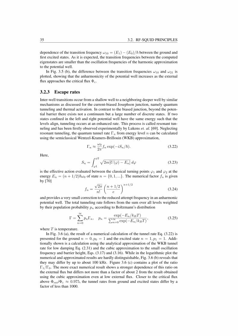
35 3.2. RF-SQUID PRINCIPLES
dependence of the transition frequency ω10 = (E1)− (E0)/~ between the ground andfirst excited states. As it is expected, the transition frequencies between the computedeigenstates are smaller than the oscillation frequencies of the harmonic approximationto the potential well.
In Fig. 3.5 (b), the difference between the transition frequencies ω10 and ω21 isplotted, showing that the anharmonicity of the potential well increases as the externalflux approaches the critical flux Φc.
3.2.3 Escape ratesInter-well transitions occur from a shallow well to a neighboring deeper well by similarmechanisms as discussed for the current-biased Josephson junction, namely quantumtunneling and thermal activation. In contrast to the biased junction, beyond the poten-tial barrier there exists not a continuum but a large number of discrete states. If twostates confined in the left and right potential well have the same energy such that thelevels align, tunneling occurs at an enhanced rate. This process is called resonant tun-neling and has been firstly observed experimentally by Lukens et. al. [69]. Neglectingresonant tunneling, the quantum tunnel rate Γn from energy level n can be calculatedusing the semiclassical Wentzel-Kramers-Brillouin (WKB) approximation,
Γn ≈ ω0
2πfn exp(−iSn/~). (3.22)
Here,
Sn =∫ ϕ2
ϕ1
√2m[U(ϕ)− En] dϕ (3.23)
is the effective action evaluated between the classical turning points ϕ1 and ϕ2 at theenergy En = (n + 1/2)~ω0 of state n = 0, 1, .... The numerical factor fn is givenby [70]
fn =√
2π
n!
(n + 1/2
e
)n+1/2
(3.24)
and provides a very small correction to the reduced attempt frequency in an anharmonicpotential well. The total tunneling rate follows from the sum over all levels weightedby their population probability pn according to Boltzmann’s distribution
Γ =∞∑
n=0
pnΓn, pn =exp(−En/kBT )∑∞
n=0 exp(−En/kBT ), (3.25)
where T is temperature.In Fig. 3.6 (a), the result of a numerical calculation of the tunnel rate Eq. (3.22) is
presented for the ground n = 0, p0 = 1 and the excited state n = 1, p1 = 1. Addi-tionally shown is a calculation using the analytical approximation of the WKB tunnelrate for low damping Eq. (2.31) and the cubic approximation to the small oscillationfrequency and barrier height, Eqs. (3.17) and (3.16). While in the logarithmic plot thenumerical and approximated results are hardly distinguishable, Fig. 3.6 (b) reveals thatthey may differ by up to about 100 kHz. Figure 3.6 (c) contains a plot of the ratioΓ1/Γ0. The more exact numerical result shows a stronger dependence of this ratio onthe external flux but differs not more than a factor of about 2 from the result obtainedusing the cubic approximation even at low external flux. Closer to the critical fluxabove Φext/Φc ≈ 0.975, the tunnel rates from ground and excited states differ by afactor of less than 1000.

CHAPTER 3. THE FLUX-BIASED PHASE QUBIT 36
100
105
1010
0.94 0.95 0.96 0.97
1010
100
105
103
cubic approximation
WKB
Γ1
Γ0
Γ1 / Γ0
Γ (WKB) - Γ (cubic approx.)1 1
Γ (cubic approx.) - Γ (WKB)0 0
(a)
(b)
(c)
Φ /Φcext
[s
]-1
[s
]-1
Figure 3.6: (a) Rates of quantum tunneling from the ground state and the first excitedstate in an rf-SQUID. Solid lines are computed numerically and dashed lines are ob-tained using the cubic approximation. (b) Difference between numerical and approxi-mated results for the ground state rate Γ0 (solid line) and the excited state Γ1 (dashedline). (c) Ratio of the tunnel rates Γ1/Γ0, calculated numerically (solid line) and usingthe cubic approximation (dashed line). Sample parameters were Ic = 1.7 µA, L = 0.72nH and C = 0.7 pF for comparability to [68] and are similar to sample UCSB-SiN.

37 3.3. QUBIT OPERATION
3.3 Qubit operationThe operation of the single junction interferometer as a phase qubit is accomplishedby applying a flux bias sequence composed of dc- and microwave frequency signals asillustrated in Fig. 3.7. In this section, an overview of the necessary steps is given, whilequbit measurement and flux state readout are discussed in more detail in Sec. 4.3 andSec. 3.4, respectively.
q
I DC_SQ
Φ
0
time
dc-pulse
0
µW-pulse
sequence
0 >
1 ωR>
01ν Γ1, DC
Γ1
resetprepare
qubit op
measurement
readout
h
reset
0 >
1 >
freeze
Iµw
Figure 3.7: Top: Timing profile of the magnetic flux bias Φq applied to the qubit.Bottom: Bias current sent to the readout SQUID.
I) Initialization. To initialize the qubit, its flux state is reset to a defined value andits phase state to the one of lowest energy in the corresponding potential well.Given that the parameter βL < 4.6, it suffices to switch the applied magneticflux to zero such that only a single potential well remains. Keeping this fluxlevel for a time much larger than the energy relaxation time T1 ensures that thequbit is initialized in the ground state |0〉. For larger values of βL > 4.6 thereexist always more than one potential minima. Initialization in a certain well inthis case is still possible by using the so-called ’shaker’ technique [71], in whichan oscillating external flux is applied to induce escape from all potential wells ofhigher energy towards the global minimum.
II) Preparation. The external flux Φq is adjusted adiabatically to a value near thecritical flux Φc to make the potential well in which the phase is confined veryshallow. While the exact value of Φq can be chosen to result in the desiredenergy difference between the two qubit states, it underlies two limitations. Onthe one hand, it must not be too large such that the first excited state does notescape from the shallow well during the qubit operation. On the other hand, asmaller value of Φc results in a deeper potential well which is more harmonic, i.e.the transition frequencies between neighboring states are less distinct from eachother. The external flux must hence be large enough to result in a potential well

CHAPTER 3. THE FLUX-BIASED PHASE QUBIT 38
of sufficient anharmonicity, ensuring that higher excited states are not populatedby a microwave tuned to the |0〉 to |1〉 transition frequency.
III) Qubit operation. After the external flux has reached the working point, logi-cal qubit operations are performed by a sequence of dc-currents and resonantmicrowave pulses. Since microwave pulses of frequency ωµw = E1 − E0/~change the individual state population undergoing Rabi oscillation, they can beused to realize the Haddamard transformation and the logical NOT gate. A dc-pulse can be used to implement the phase gate by introducing a small detuningwhich changes the Larmor frequency and hence the precession velocity of theBloch vector.
IV) Qubit measurement. After sending the microwave pulse, a short but still adia-batic dc-flux pulse is applied which raises the excited state close to the top ofthe potential barrier. It is possible to adjust the amplitude and duration of thismeasurement pulse such that only the excited state tunnels to the deep right well,whereas the ground state remains in the shallow left well. Thereby, the phaseeigenstates |0〉 and |1〉 are mapped to macroscopically distinct flux states in theshallow and deep wells, respectively. This technique [34] allows to distinguishthe phase eigenstates with a fidelity [68] close to 100 %.
IV) State readout. After application of the measurement dc-pulse, the applied mag-netic flux is reduced, hereby increasing the barrier height separating the twowells in order to avoid further inter-well transitions. Whether the qubit is nowin the left or right well is determined by measuring the corresponding magneticfield in the qubit loop by means of an inductively coupled dc-SQUID.
3.4 ReadoutSeveral methods can be used to measure the flux state of the phase qubit. One of them[72] directly determines the circulation direction of the loop current by a measurementof the critical current of an additional junction incorporated in the loop. Less invasivetechniques are based on a measurement of the flux generated from the loop current byusing an inductively coupled dc-SQUID. In this section, the circuit design requirementsfor the widely used method of flux detection by a switching-current measurement ofthe dc-SQUID are discussed. Beyond that, the principles of a dispersive readout basedon a measurement of the dc-SQUID inductance are presented as an outlook.
3.4.1 Principles of the dc-SQUIDA dc-SQUID consists of two Josephson junctions embedded in a superconductingloop [8, 9] as shown in Fig. (3.8).
From the flux quantization condition, the relation between the phase differencesacross the two junctions ϕ1 and ϕ2 is found as
ϕ1 − ϕ2 =2π
Φ0Φsq =
2π
Φ0(Φa + LJ), (3.26)
where the flux in the dc-SQUID loop Φsq has contributions from the externally appliedflux Φa and the flux generated from the current J circulating in the loop of inductanceLsq= L1 +L2. An applied bias current Ib distributes among junctions 1 and 2 equally,
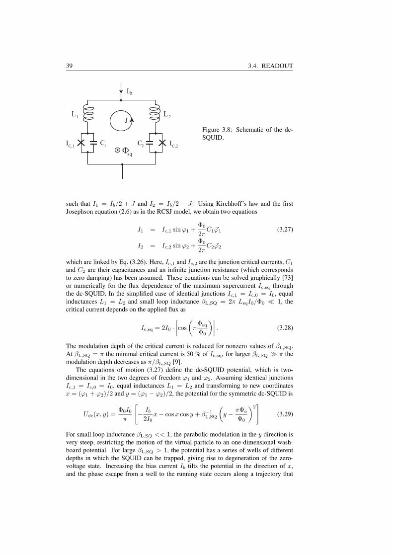
39 3.4. READOUT
L
XC
Ib
Φsq
IC,22
2L
X CIC,1 1
1J
Figure 3.8: Schematic of the dc-SQUID.
such that I1 = Ib/2 + J and I2 = Ib/2 − J . Using Kirchhoff’s law and the firstJosephson equation (2.6) as in the RCSJ model, we obtain two equations
I1 = Ic,1 sin ϕ1 +Φ0
2πC1ϕ1 (3.27)
I2 = Ic,2 sin ϕ2 +Φ0
2πC2ϕ2
which are linked by Eq. (3.26). Here, Ic,1 and Ic,2 are the junction critical currents, C1
and C2 are their capacitances and an infinite junction resistance (which correspondsto zero damping) has been assumed. These equations can be solved graphically [73]or numerically for the flux dependence of the maximum supercurrent Ic,sq throughthe dc-SQUID. In the simplified case of identical junctions Ic,1 = Ic,0 = I0, equalinductances L1 = L2 and small loop inductance βL,SQ = 2π LsqI0/Φ0 ¿ 1, thecritical current depends on the applied flux as
Ic,sq = 2I0 ·∣∣∣∣cos
(π
Φsq
Φ0
)∣∣∣∣ . (3.28)
The modulation depth of the critical current is reduced for nonzero values of βL,SQ.At βL,SQ = π the minimal critical current is 50 % of Ic,sq, for larger βL,SQ À π themodulation depth decreases as π/βL,SQ [9].
The equations of motion (3.27) define the dc-SQUID potential, which is two-dimensional in the two degrees of freedom ϕ1 and ϕ2. Assuming identical junctionsIc,1 = Ic,0 = I0, equal inductances L1 = L2 and transforming to new coordinatesx = (ϕ1 + ϕ2)/2 and y = (ϕ1 − ϕ2)/2, the potential for the symmetric dc-SQUID is
Udc(x, y) =Φ0I0
π
[− Ib
2I0x− cos x cos y + β−1
L,SQ
(y − πΦa
Φ0
)2]
(3.29)
For small loop inductance βL,SQ << 1, the parabolic modulation in the y direction isvery steep, restricting the motion of the virtual particle to an one-dimensional wash-board potential. For large βL,SQ > 1, the potential has a series of wells of differentdepths in which the SQUID can be trapped, giving rise to degeneration of the zero-voltage state. Increasing the bias current Ib tilts the potential in the direction of x,and the phase escape from a well to the running state occurs along a trajectory that

CHAPTER 3. THE FLUX-BIASED PHASE QUBIT 40
connects the minimum of the well with the lowest saddle point in the vicinity. For acertain zero-voltage state, the critical current Ic,sq can be found from a potential anal-ysis by imposing the constraint that at Ib = Ic,sq the minimum of one well coincideswith a neighboring saddle point [74]. Any asymmetry in either the critical current of thetwo junctions or the inductances between the two branches results in a shift of the fluxvalue where the critical current of the SQUID is maximum [75]. Experimental data ofthe mean switching current dependence on external flux, obtained from an asymmetricdc-SQUID of βL,SQ ≈ 25 and critical current Ic,sq ≈ 21.8µA, is shown in Fig. 3.9.
8
10
12
14
16
18
20
-0.8 -0.6 -0.4 -0.2 0 0.2 0.4 0.6 0.8
magnetic field [Φ ]
swit
chin
g c
urr
ent
[µ A
]
0
Figure 3.9: Switching currents vs. magnetic bias flux for an asymmetric and large in-ductance dc-SQUID. The grey scale reflects the switching probability, increasing fromwhite to black. At a given bias flux, several peaks in the switching-current distribu-tion reflect the degeneracy of the zero-voltage state in the two dimensional washboardpotential. Sample: Hyp100.
During operation of the phase qubit, the bias current of the dc-SQUID is set to avalue that minimizes the coupling between the dc-SQUID’s degree of freedom and theflux that it receives from the qubit [76]. For example, a symmetric dc-SQUID of lowinductance βL,SQ < 1 can be described by a single degree of freedom ϕsq, which isrelated to its bias current by the Josephson relation
Isq = Ic,sq sin ϕsq = 2I0 ·∣∣∣∣cos
(π
Φsq
Φ0
)∣∣∣∣ sin ϕsq, (3.30)
where Eq. 3.28 is used. Solving this equation for ϕsq results in
ϕsq = sin−1
[Isq
2I0
∣∣∣∣cos(
πΦsq
Φ0
)∣∣∣∣−1
], (3.31)

41 3.4. READOUT
which shows that for zero bias current Isq = 0 the dc-SQUID phase ϕsq is not cor-related to the external flux Φsq and hence the dc SQUID remains isolated from thequbit.
3.4.2 Switching-current readoutAs it was described before, after the logical qubit operations its phase eigenstates areprojected into separate wells of the qubit potential which differ by one flux quantumin the qubit loop. In this section, I describe design requirements and methods of dataevaluation which allow to detect this flux signal by switching-current measurements ona readout dc-SQUID.
X
X X
MR
V
Φq Φsq
Isq
Figure 3.10: Schematic of the phase qubitsystem. The coil in the left part of the fig-ure provides bias magnetic flux Φq to thequbit. The junction in the qubit loop is ca-pacitively coupled to a microwave sourcefor resonant qubit control. The dc-SQUIDis coupled to the qubit loop by the mutualinductance MR to read out the qubit fluxstate by a switching-current measurement.
Fig. 3.10 shows that the readout dc-SQUID is coupled by the mutual inductanceMR to the qubit loop. The flux signal that must be detectable is
∆Φsq = MR∆Iq ≈ MR
LΦ0, (3.32)
where ∆Iq ≈ Ic (see Fig. 3.2) is the change of the circulating current associated to achange of the qubit potential well. For the reasons discussed in section 3.1.4, sufficientqubit isolation requires the ratio MR/L to be ≈ 10−2, which limits the flux signal∆Φsq to the order of 10 mΦ0. The method to detect this small flux change is based onthe magnetic field dependence of the dc-SQUID critical current Ic,sq, which is periodicin Φ0 as discussed in the preceding section.
The most direct way to determine Ic,sq is to record the statistical probability distri-bution P (Ib) of bias currents Isw at which the SQUID switches to the non-zero voltagestate. In a widely used method [77], a linear current ramp dIb/dt is used, in which casethe switching-current histogram takes the form
P (Ib) = Γ(Ib,Φa)(
dIb
dt
)−1(
1−∫ I
0
P (I ′) dI ′)
. (3.33)
Here, Γ(Ib,Φa) is the escape rate from the superconducting state which depends ex-ponentially on the critical current Ic,sq and thus on the flux in the dc-SQUID Φa. Theresult of a numerical calculation of the histogram Eq. (3.33), using the quantum tunnelrate Eq. (2.31), is shown in Fig. 3.11 (a).
In order to detect flux changes, a practically useful observable is the mean switch-ing current 〈Isw〉, which directly relates to the SQUID critical current. The statistical

CHAPTER 3. THE FLUX-BIASED PHASE QUBIT 42
spread σ (the standard deviation which is also the width of the probability distributionhistogram P (Ib)) originates in the probabilistic nature of the switching process, andhas contributions from quantum, thermal and bias current fluctuations [78].
0.94 0.96 0.98
0
50
100
150
200
Switching current I sw [µ A]
P(I)
0 2 4 6 8 10
2
4
6
8
Capacitance [pF]
[nA
]
0.85
0.9
0.95
1
C = 1 pF
C = 4 pF
σ
I< >swσ
(a) (b)
I<
>sw
[µ A
]
Figure 3.11: (a) Switching current distributions P (Isw) for a single small Josephsonjunction of 1 µA critical current with capacitances of C=1 pF (left histogram) and C=4pF (right histogram). The corresponding mean switching currents are indicated by ver-tical dashed lines, and the standard deviations σ by horizontal lines at half the histogramheight. (b) Dependence of the histogram width σ (left axis) and mean switching cur-rent (right axis). Both plots are calculated from the quantum tunnel rate Eq. (2.31) anda ramp rate of 1 mA/s.
Single-shot readout
In order to distinguish the two qubit flux states |L〉 and |R〉 at maximum contrast, thehistograms P (Ib) corresponding to these states must not overlap. If this criterium isfulfilled, it becomes possible to determine by a single switching current measurementwhether the qubit was in the left or right well. This so-called single shot readout re-quires the flux difference ∆Φsq to result in a shift of the mean switching current ∆Isw
which is at least about four times larger than the standard deviation (see Fig. 3.12).Using Eq. (3.32), the single-shot criterium can be written as
∆Isw =MR
L
∂Isw
∂Φa& 4σ, (3.34)
In this formula, ∂Isw/∂Φa is the change of the mean switching current with flux inthe dc-SQUID, which depends on the working point and is zero at the maximum ofthe Ic,sq(Φa) relation. Large values of βL,SQ, which may be necessary to achieve therequired mutual inductance MR, reduce the modulation of the mean switching currentas discussed in the previous section.
The mutual inductance mediates dissipation in the dc-SQUID and generates back-action to the qubit. While the back-action scales as M2
R/LLsq, dissipation in the qubitis proportional to the inverse effective dc-SQUID damping impedance Z−1
sq , which istransformed to the qubit via Z−1 = Z−1
sq (MR/L)2. A detailed discussion of decoher-ence effects due to coupling to the readout SQUID is given in Ref. [76].
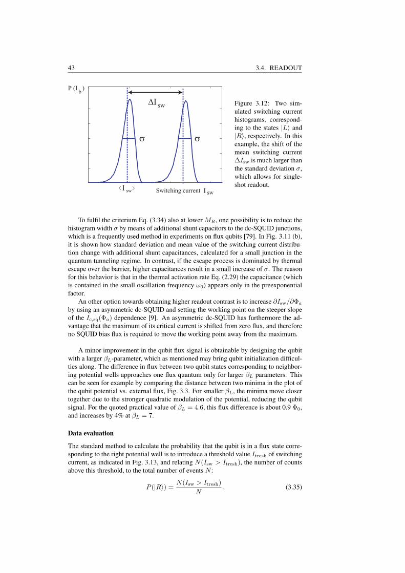
43 3.4. READOUT
P (I )
σ
∆I sw
Switching current I sw
b
σ
I< >sw
Figure 3.12: Two sim-ulated switching currenthistograms, correspond-ing to the states |L〉 and|R〉, respectively. In thisexample, the shift of themean switching current∆Isw is much larger thanthe standard deviation σ,which allows for single-shot readout.
To fulfil the criterium Eq. (3.34) also at lower MR, one possibility is to reduce thehistogram width σ by means of additional shunt capacitors to the dc-SQUID junctions,which is a frequently used method in experiments on flux qubits [79]. In Fig. 3.11 (b),it is shown how standard deviation and mean value of the switching current distribu-tion change with additional shunt capacitances, calculated for a small junction in thequantum tunneling regime. In contrast, if the escape process is dominated by thermalescape over the barrier, higher capacitances result in a small increase of σ. The reasonfor this behavior is that in the thermal activation rate Eq. (2.29) the capacitance (whichis contained in the small oscillation frequency ω0) appears only in the preexponentialfactor.
An other option towards obtaining higher readout contrast is to increase ∂Isw/∂Φa
by using an asymmetric dc-SQUID and setting the working point on the steeper slopeof the Ic,sq(Φa) dependence [9]. An asymmetric dc-SQUID has furthermore the ad-vantage that the maximum of its critical current is shifted from zero flux, and thereforeno SQUID bias flux is required to move the working point away from the maximum.
A minor improvement in the qubit flux signal is obtainable by designing the qubitwith a larger βL-parameter, which as mentioned may bring qubit initialization difficul-ties along. The difference in flux between two qubit states corresponding to neighbor-ing potential wells approaches one flux quantum only for larger βL parameters. Thiscan be seen for example by comparing the distance between two minima in the plot ofthe qubit potential vs. external flux, Fig. 3.3. For smaller βL, the minima move closertogether due to the stronger quadratic modulation of the potential, reducing the qubitsignal. For the quoted practical value of βL = 4.6, this flux difference is about 0.9 Φ0,and increases by 4% at βL = 7.
Data evaluation
The standard method to calculate the probability that the qubit is in a flux state corre-sponding to the right potential well is to introduce a threshold value Itresh of switchingcurrent, as indicated in Fig. 3.13, and relating N(Isw > Itresh), the number of countsabove this threshold, to the total number of events N :
P (|R〉) =N(Isw > Itresh)
N. (3.35)

CHAPTER 3. THE FLUX-BIASED PHASE QUBIT 44
3.33.12.9
0
0.2
0.4
0.6
0.8
1
external flux [a.u.]
8 9
0
1
2
3
switching current I [µA]sw
70 % 100 %
(a) (b)
P(I) R>P ( )
Ithresh
Figure 3.13: (a) Switching current distributions which are broadened due to thermalactivation. Left and right histograms correspond to the qubit being in state |R〉 and |L〉,respectively. The smaller histogram corresponds to equal probability of the two states.Dashed lines are polynomial fits. (b) The probability to measure the state |R〉 versusexternally applied flux. The blue dotted curve is calculated using the standard method,resulting in a maximum contrast of 70%. The red solid curve has been obtained fromweighted fits to the histograms, and reconstructs the two states with 100% contrast.
If the two histograms are not completely separated, switching current events in theregion of histogram overlap can not be attributed to one or the other state, and loss ofcontrast occurs. This is shown in Fig. 3.13 (b) as the dashed curve calculated accordingto Eq. (3.35).
In practical qubit measurements, statistics about the state population are alwaysacquired because of the probabilistic nature of quantum mechanics. A single shotmeasurement is therefore not necessary as long as it is still possible to reconstruct theindividual state contribution from the statistical data set.
Our method to reconstruct the qubit state population from overlapping histogramsbeyond the single shot limit is the following. The qubit is first prepared in state |L〉,recording the switching current probability histogram P (I) generated by only thisstate. This histogram is fitted to an arbitrary function fL(I). For simplicity, we are us-ing a 10 degree polynomial truncated between minimal and maximal measured switch-ing currents as the fitting function. Fitting to a physically correct distribution, whichis an integral function of the exponential escape rate, would require more computingtime and an adaption of the model depending on the sample. The same procedure isrepeated on a histogram obtained from measurements of a qubit prepared purely in thestate |R〉, obtaining the fitting function fR(I). All further histograms are then fitted tothe function
P (I) = P (|1〉) fR(I) + [1− P (|1〉)] fL(I), (3.36)
hereby obtaining P (|1〉), the population of the excited qubit state |1〉, as the only fittingparamter.
In Fig. 3.13 (a), histograms of the qubit prepared in state |L〉, |R〉 and in a superpo-sition state are shown together with the fitting functions drawn as dashed lines. Figure
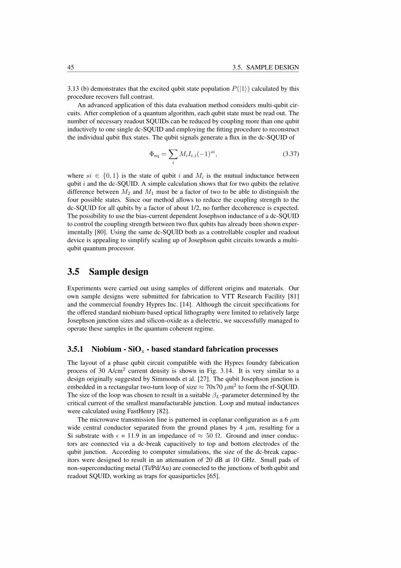
45 3.5. SAMPLE DESIGN
3.13 (b) demonstrates that the excited qubit state population P (|1〉) calculated by thisprocedure recovers full contrast.
An advanced application of this data evaluation method considers multi-qubit cir-cuits. After completion of a quantum algorithm, each qubit state must be read out. Thenumber of necessary readout SQUIDs can be reduced by coupling more than one qubitinductively to one single dc-SQUID and employing the fitting procedure to reconstructthe individual qubit flux states. The qubit signals generate a flux in the dc-SQUID of
Φsq =∑
i
MiIc,i(−1)si, (3.37)
where si ∈ 0, 1 is the state of qubit i and Mi is the mutual inductance betweenqubit i and the dc-SQUID. A simple calculation shows that for two qubits the relativedifference between M2 and M1 must be a factor of two to be able to distinguish thefour possible states. Since our method allows to reduce the coupling strength to thedc-SQUID for all qubits by a factor of about 1/2, no further decoherence is expected.The possibility to use the bias-current dependent Josephson inductance of a dc-SQUIDto control the coupling strength between two flux qubits has already been shown exper-imentally [80]. Using the same dc-SQUID both as a controllable coupler and readoutdevice is appealing to simplify scaling up of Josephson qubit circuits towards a multi-qubit quantum processor.
3.5 Sample designExperiments were carried out using samples of different origins and materials. Ourown sample designs were submitted for fabrication to VTT Research Facility [81]and the commercial foundry Hypres Inc. [14]. Although the circuit specifications forthe offered standard niobium-based optical lithography were limited to relatively largeJosephson junction sizes and silicon-oxide as a dielectric, we successfully managed tooperate these samples in the quantum coherent regime.
3.5.1 Niobium - SiOx - based standard fabrication processes
The layout of a phase qubit circuit compatible with the Hypres foundry fabricationprocess of 30 A/cm2 current density is shown in Fig. 3.14. It is very similar to adesign originally suggested by Simmonds et al. [27]. The qubit Josephson junction isembedded in a rectangular two-turn loop of size ≈ 70x70 µm2 to form the rf-SQUID.The size of the loop was chosen to result in a suitable βL-parameter determined by thecritical current of the smallest manufacturable junction. Loop and mutual inductanceswere calculated using FastHenry [82].
The microwave transmission line is patterned in coplanar configuration as a 6 µmwide central conductor separated from the ground planes by 4 µm, resulting for aSi substrate with ε = 11.9 in an impedance of ≈ 50 Ω. Ground and inner conduc-tors are connected via a dc-break capacitively to top and bottom electrodes of thequbit junction. According to computer simulations, the size of the dc-break capac-itors were designed to result in an attenuation of 20 dB at 10 GHz. Small pads ofnon-superconducting metal (Ti/Pd/Au) are connected to the junctions of both qubit andreadout SQUID, working as traps for quasiparticles [65].

CHAPTER 3. THE FLUX-BIASED PHASE QUBIT 46
bottom layer
top layer
junction
via
qubit
dc-SQUIDdc-break
microwave line
flux bias coil quasiparticle trap
100 µm
Figure 3.14: Design of sample Hyp30 for the 30 A/cm2 Hypres process.
The size and position of the readout dc-SQUID loop were chosen to result in asufficiently large mutual inductance, typically about 10 pH, to allow detection of thequbit flux state in a single-shot measurement, as discussed in Sec. 3.4.2. The bias andvoltage lines are connected symmetrically to the dc-SQUID loop such that an appliedbias current would divide equally between the two branches if their inductances wereequal. In this case, no net magnetic flux is generated in the qubit loop and the qubitremains protected from fluctuations in the dc-SQUID bias current. To keep this advan-tage for an asymmetric dc-SQUID, in one branch of the dc-SQUID a single junction isplaced, while the other branch contains a series combination of two junctions of twicethe critical current each [27]. Since the Josephson inductance Eq. (2.11) is inverselyproportional to the critical current, a series combination of two junctions has the sameinductance as a single smaller junction of half the critical current. Thus, as long as nobias current is applied, the SQUID remains symmetric.
The coil to apply bias flux to the qubit is designed gradiometrically in the form ofan ’8’, so that the current will flow as indicated by the arrows in Fig. 3.14. The read-out dc-SQUID is placed symmetrically with respect to this biasing coil such that theflux received from each half of the ’8’-shaped coil is of same magnitude but oppositedirection. This cancels changes of the dc-SQUID operation point when the qubit fluxis varied.
The mutual inductance Mqb between qubit and flux bias coil was chosen to beMqb ≈ 2 pH, such that a coil current of 1 mA results in an induced qubit flux ofabout one Φ0. Although a smaller mutual inductance would increase qubit isolation,it is impractical to apply larger currents to on-chip coils due to the risk of heatingthe sample. While the risk of exceeding the critical current of thin superconductingfilms is limited by designing the flux line with a larger width, heating in the non-superconducting wire sections which are thermally anchored to the mixing chambermay be strong enough to increase the reachable base temperature by tens of milikelvin.

47 3.5. SAMPLE DESIGN
The dissipated power grows quadratically with the applied current. Furthermore, ifcontact resistances were present in the Aluminum bonds, heating would occur directlyon the sample chip [60].
bottom layertop layer
junctionvia
bonding pad
microwave line qubitreadout
dc-SQUID
flux bias
coil
100 µm
Figure 3.15: Design of sample VTT30 for the 30 A/cm2 VTT process.
Gradiometric design
Fluctuations of the magnetic field experienced by the qubit may constitute a relevantsource of decoherence. They give rise to a low-frequency fluctuation of the energy levelseparation, resulting in dephasing. Since the qubit loop must be made large enough toobtain the required inductance, this device is more sensitive to field fluctuations thanflux qubits, in which the geometric inductance is replaced by the Josephson inductanceof additional junctions [59, 11, 83]. The fluctuations can be due to vibrational motionof the sample in the background (earth) magnetic field, or can be generated by ac powerlines and vacuum pumps in the vicinity of the sample.
A geometric solution to this problem is to redesign the phase qubit system withgradiometric coils. Figure 3.16 shows an improved layout, in which the rf-SQUIDinductance is drawn in the shape of an ’8’, which can be seen as a single coil whoseopposite halves are twisted by 180o. A homogenous external field will not induce anyscreening currents in such a coil since the current driving force is opposite in eachof its two halves which will hence cancel each other. To be able to read out the fluxinside this twisted loop, the dc-SQUID (seen as the smaller ’8’-shaped structure tothe right of the qubit) was also designed in a gradiometric configuration. This has theadditional advantage of immunity to background field fluctuations also for the readoutSQUID. The wires to current-bias the dc-SQUID are connected in the middle of the ’8’-shape, where bottom and top metalization layers overlap. By visualizing the directionof the bias current flow in the dc-SQUID, one can see that current fluctuations of equalamplitude in both branches will not affect the qubit. In contrast to the non-gradiometric
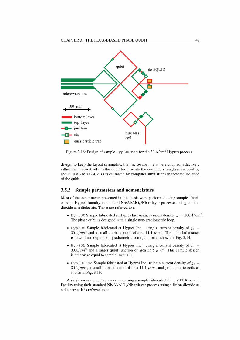
CHAPTER 3. THE FLUX-BIASED PHASE QUBIT 48
bottom layer
top layer
junction
via
quasiparticle trap
100 µm
microwave line
qubitdc-SQUID
flux bias
coil
Figure 3.16: Design of sample Hyp30Grad for the 30 A/cm2 Hypres process.
design, to keep the layout symmetric, the microwave line is here coupled inductivelyrather than capacitively to the qubit loop, while the coupling strength is reduced byabout 10 dB to ≈ -30 dB (as estimated by computer simulation) to increase isolationof the qubit.
3.5.2 Sample parameters and nomenclatureMost of the experiments presented in this thesis were performed using samples fabri-cated at Hypres foundry in standard Nb/Al/AlOx/Nb trilayer processes using siliciondioxide as a dielectric. Those are referred to as
• Hyp100 Sample fabricated at Hypres Inc. using a current density jc = 100A/cm2.The phase qubit is designed with a single non-gradiometric loop.
• Hyp30S Sample fabricated at Hypres Inc. using a current density of jc =30A/cm2 and a small qubit junction of area 11.1 µm2. The qubit inductanceis a two-turn loop in non-gradiometric configuration as shown in Fig. 3.14.
• Hyp30L Sample fabricated at Hypres Inc. using a current density of jc =30A/cm2 and a larger qubit junction of area 35.5 µm2. This sample designis otherwise equal to sample Hyp100.
• Hyp30Grad Sample fabricated at Hypres Inc. using a current density of jc =30A/cm2, a small qubit junction of area 11.1 µm2, and gradiometric coils asshown in Fig. 3.16.
A single measurement run was done using a sample fabricated at the VTT ResearchFacility using their standard Nb/Al/AlOx/Nb trilayer process using silicion dioxide asa dielectric. It is referred to as
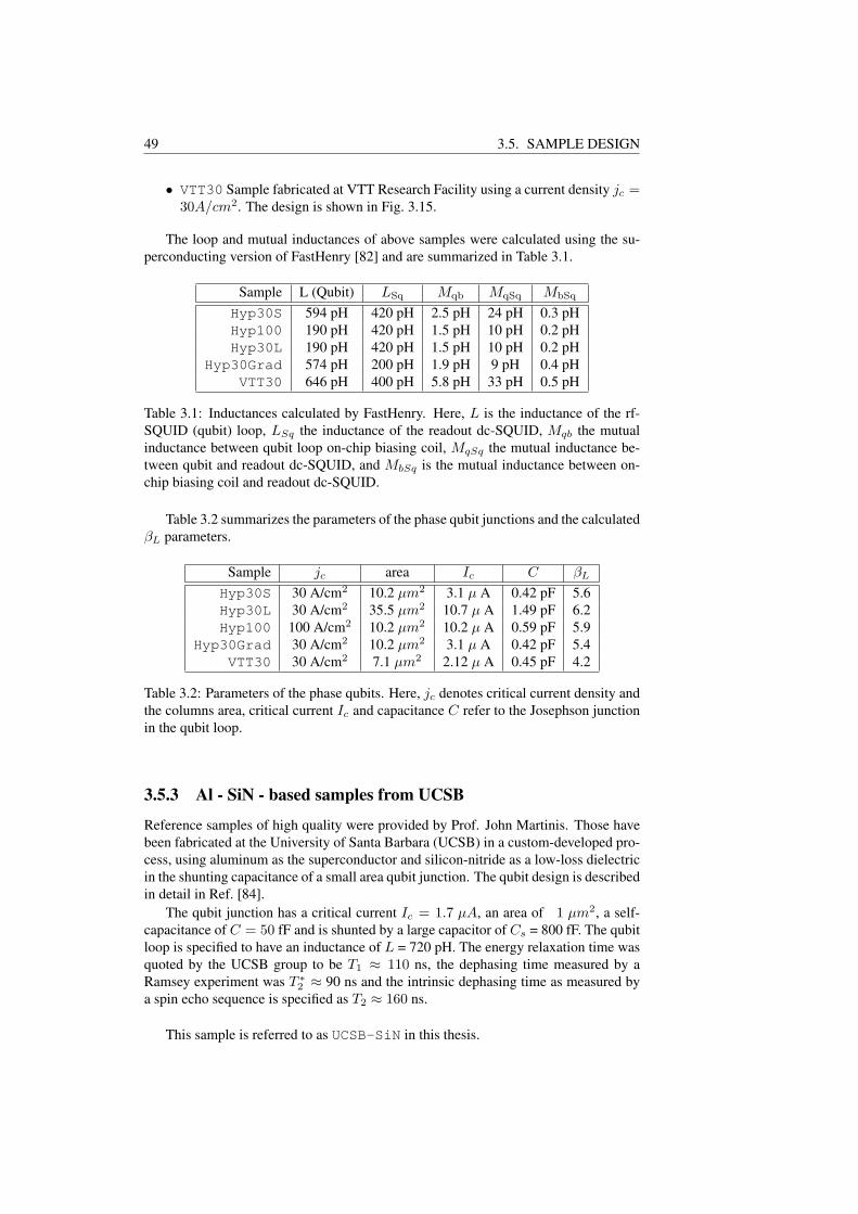
49 3.5. SAMPLE DESIGN
• VTT30 Sample fabricated at VTT Research Facility using a current density jc =30A/cm2. The design is shown in Fig. 3.15.
The loop and mutual inductances of above samples were calculated using the su-perconducting version of FastHenry [82] and are summarized in Table 3.1.
Sample L (Qubit) LSq Mqb MqSq MbSq
Hyp30S 594 pH 420 pH 2.5 pH 24 pH 0.3 pHHyp100 190 pH 420 pH 1.5 pH 10 pH 0.2 pHHyp30L 190 pH 420 pH 1.5 pH 10 pH 0.2 pH
Hyp30Grad 574 pH 200 pH 1.9 pH 9 pH 0.4 pHVTT30 646 pH 400 pH 5.8 pH 33 pH 0.5 pH
Table 3.1: Inductances calculated by FastHenry. Here, L is the inductance of the rf-SQUID (qubit) loop, LSq the inductance of the readout dc-SQUID, Mqb the mutualinductance between qubit loop on-chip biasing coil, MqSq the mutual inductance be-tween qubit and readout dc-SQUID, and MbSq is the mutual inductance between on-chip biasing coil and readout dc-SQUID.
Table 3.2 summarizes the parameters of the phase qubit junctions and the calculatedβL parameters.
Sample jc area Ic C βL
Hyp30S 30 A/cm2 10.2 µm2 3.1 µ A 0.42 pF 5.6Hyp30L 30 A/cm2 35.5 µm2 10.7 µ A 1.49 pF 6.2Hyp100 100 A/cm2 10.2 µm2 10.2 µ A 0.59 pF 5.9
Hyp30Grad 30 A/cm2 10.2 µm2 3.1 µ A 0.42 pF 5.4VTT30 30 A/cm2 7.1 µm2 2.12 µ A 0.45 pF 4.2
Table 3.2: Parameters of the phase qubits. Here, jc denotes critical current density andthe columns area, critical current Ic and capacitance C refer to the Josephson junctionin the qubit loop.
3.5.3 Al - SiN - based samples from UCSB
Reference samples of high quality were provided by Prof. John Martinis. Those havebeen fabricated at the University of Santa Barbara (UCSB) in a custom-developed pro-cess, using aluminum as the superconductor and silicon-nitride as a low-loss dielectricin the shunting capacitance of a small area qubit junction. The qubit design is describedin detail in Ref. [84].
The qubit junction has a critical current Ic = 1.7 µA, an area of 1 µm2, a self-capacitance of C = 50 fF and is shunted by a large capacitor of Cs = 800 fF. The qubitloop is specified to have an inductance of L = 720 pH. The energy relaxation time wasquoted by the UCSB group to be T1 ≈ 110 ns, the dephasing time measured by aRamsey experiment was T ∗2 ≈ 90 ns and the intrinsic dephasing time as measured bya spin echo sequence is specified as T2 ≈ 160 ns.
This sample is referred to as UCSB-SiN in this thesis.

CHAPTER 3. THE FLUX-BIASED PHASE QUBIT 50
3.6 Experimental technique
3.6.1 Wiring and filtering
A prominent feature of superconducting qubits is the opportunity to control them con-veniently through directly attached wires. However, strong coupling to environmen-tal degrees of freedom via these wires and fluctuations in the biasing signals presentsources of decoherence. As a particular challenge, the control circuitry must be de-signed to protect the qubit from noise sources and on the other hand provide the chan-nels to control and monitor the qubit state.
A single phase qubit requires three signal channels. Two of them serve to controlthe qubit by transmitting magnetic flux bias and microwave currents. The third is thereadout channel, which is connected to the dc-SQUID. To reduce the noise level, astandard technique is to narrow the bandwidth of the signal cables. However, this isnot an option for the flux line, because it serves to both control the level of constantmagnetic bias flux and to transmit dc-pulses as short as one nanosecond to allow forfast control of the Larmour frequency and state readout. The microwave line must betransparent in a wide frequency range up to the qubit resonance frequency of up to 20GHz, but can be equipped with a dc-break acting as a high-pass filter. Therefore, forqubit control we use standard coaxial cables of a certified bandwidth of 18 GHz, butreduce the noise by coupling them very weakly to the qubit. Moreover, to increasethe signal-to-noise ratio, both these lines are equipped with SMA-type attenuators [85]of 10 dB at the 1.4 K temperature stage, while the microwave line uses an additional10 dB attenuator at the sample temperature. In earlier experiments, we noticed that astrong parasitic resonance occurring in the microwave line was due to attenuators [86]which became superconducting at temperatures below about 0.8 K.
The bias line of the readout dc-SQUID is designed to have a bandwidth limited toabout 5 KHz. As shown in Fig. 3.17, several filters are used at different temperaturestages. Both bias current and voltage sensing lines are equipped with commercial feed-through filters at room temperature, followed by RC-filters at 1.4 K temperature. At ashort distance to the sample chip, these lines pass through custom-made capacitivelyshunted copper powder filters which are designed to have an attenuation of more than80 dB above a frequency of 1 GHz [87]. To measure the dc-SQUID voltage differen-tially, we connect it by a twisted pair to the room temperature amplifier. The dc-SQUIDbias is sent through a single copper wire and the cryostat ground serves as the currentreturn path. A current-divider of factor ≈ 50 is inserted in the current line at the 1.4 Ktemperature stage to improve the signal-to-noise ratio. Our experience showed that thisconfiguration reduces greatly the sensitivity of the dc-SQUID measurement to noisecurrents flowing in ground loops which exist in the room temperature electronics aswell as interference from equipment powered from the mains supply when connectedto the cryostat, like oscilloscope or temperature controller.
The current-divider is realized from standard SMD resistors, which can dramati-cally change their resistances at low temperature. As a consequence, it is not knownexactly how much current is flowing through the readout dc-SQUID during the exper-iment. For qubit measurements, however, this knowledge is not required, but it alwaysremains possible to measure the current-dividing ratio by using the differential voltagelines for current-biasing and the current line for the voltage measurement.

51 3.6. EXPERIMENTAL TECHNIQUE
X X
copper-powder
filters
V
I
T = 300 K T = 1.8 K mixing chamber
240 Ω 240 Ω
10 Ω
270 Ω 270 Ω
270 Ω 270 Ω
33 nF
33 nF
66 nF
100 nH
2 nF
100 nH
2 nF
100 nH
2 nF
Figure 3.17: Schematic of the dc-SQUID wiring, consisting of EMI filters at roomtemperature, custom-made RC-filters at 1.8 K temperature, and capacitively shuntedcopper-powder filters at mixing chamber temperature.
3.6.2 Sample holder
Our sample housing is a copper cell of dimensions about 20 mm x 20 mm x 5 mm, inwhich up to four sample chips of 5x5 mm size can be glued at the same time. Mea-surements show that cavity resonance in the sample cell occurs around 8 GHz. Thincopper wires as well as six coaxial cables enter the cell from the bottom and are sol-dered to copper bonding pads surrounding the sample cell. We are using Al bondingwires of lengths up to about 5 mm to realize the connection to on-chip bonding pads,whereas those for the microwave currents are kept as short as possible and realizedby three parallel wires in a coplanar configuration. To protect the qubits from mag-netic field fluctuations, the inside of the sample housing is covered by a thin layer ofaluminum and a cylindrical lead shield surrounds the sample cell. To avoid trappingof vortices in the superconducting shields or on-chip niobium films during the cool-down, the sample holder is surrounded by two cylinders made of cryoperm [88]. Thesample holder is then thermally anchored to the mixing chamber of an Oxford Instru-ments Kelvinox He3/He4 dilution refrigerator which has a base temperature of about15 mK. The cryostat is placed in a commercial shielded room, which is grounded butgalvanically isolated from the gas handling system.
3.6.3 Electronics
The custom-made analog electronics generate the low frequency part of the qubit fluxbias, serve for dc-SQUID readout and provide an isolating interface to the externalcomputer for data acquisition. A careful grounding scheme allows to power the elec-tronics from a transformer connected to a filtered mains supply inside the shieldedroom. We found no difference in the qubit performance when the electronics wasdriven from batteries. A mains transformer greatly extends the long-term stability ofthe experiment up to several weeks. Figure 3.18 provides a schematic of the experi-

CHAPTER 3. THE FLUX-BIASED PHASE QUBIT 52
mental setup, which is explained in the following.
ON
Out
OFF
DAC
Out 1
Out 2
Out 3reset
level
field 1
level
field 2
level
TRIG
APG
flip
flop
X
trigger
STOP START
X X
ramp
generator
time
counter
STOP
CH 1
CH 2
TRIG
START
hi-speed
pulsegen
µW-source
readout-
dc-pulse
PC
XXXX XX
Figure 3.18: Schematic of the experimental setup. The measurement sequence isstarted by a trigger pulse generated by the high-speed pulse generator shown in thelower left corner.
Qubit flux bias
To operate the phase qubit, its magnetic bias flux is switched between three levels asshown in Fig. (3.7). These are a reset level, at which the qubit potential has a singleminimum, the working point, at which a shallow potential well allows to operate in thetwo-level limit, and a freeze level at which the barrier between the two wells is large.To generate the required flux sequence, we connect two current sources in parallel tothe on-chip coil. These sources are controlled by a voltage in the range of ± 10 V andgenerate currents in a switchable range of 10−2 to 10−7 A/V. The dc-voltages corre-sponding to the flux levels are delivered by a set of 16-bit precision digital-to-analogconverters [89]. These are equipped with a serial interface that allows cascading of mul-tiple converters in a daisy-chain, such that only one signal input is necessary. To avoidthe presence of digital noise in the electronics during qubit operation, the DAC clocksignal is generated by a custom-built logic circuit only throughout reprogramming thevoltage levels. The digital data are encoded in a pulse-width modulated signal, whichis created by a National Instruments output interface card in the controlling computerand sent to the DAC module via an optical fiber line featuring galvanic isolation.
As it is shown in Fig. 3.18, the desired flux level is selected by the state of twoswitches which connect the current source control input to different DAC voltage out-puts. These are realized by an integrated circuit of analog switches [90] which are
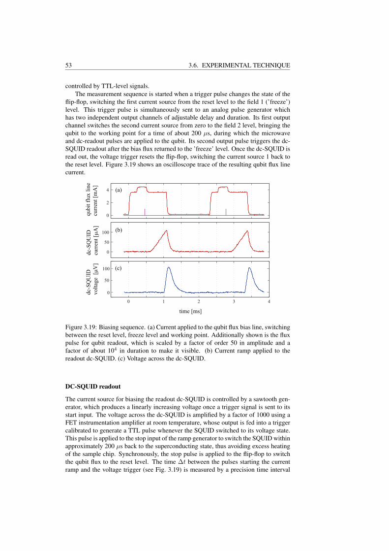
53 3.6. EXPERIMENTAL TECHNIQUE
controlled by TTL-level signals.The measurement sequence is started when a trigger pulse changes the state of the
flip-flop, switching the first current source from the reset level to the field 1 (’freeze’)level. This trigger pulse is simultaneously sent to an analog pulse generator whichhas two independent output channels of adjustable delay and duration. Its first outputchannel switches the second current source from zero to the field 2 level, bringing thequbit to the working point for a time of about 200 µs, during which the microwaveand dc-readout pulses are applied to the qubit. Its second output pulse triggers the dc-SQUID readout after the bias flux returned to the ’freeze’ level. Once the dc-SQUID isread out, the voltage trigger resets the flip-flop, switching the current source 1 back tothe reset level. Figure 3.19 shows an oscilloscope trace of the resulting qubit flux linecurrent.
0
2
4
0
50
100
0 1 2 3 4
(a)
(b)
(c)
qu
bit
flu
x l
ine
curr
ent
[mA
]d
c-S
QU
ID
curr
ent
[µA
]
dc-
SQ
UID
vo
ltag
e [µ
V]
0
50
100
time [ms]
Figure 3.19: Biasing sequence. (a) Current applied to the qubit flux bias line, switchingbetween the reset level, freeze level and working point. Additionally shown is the fluxpulse for qubit readout, which is scaled by a factor of order 50 in amplitude and afactor of about 104 in duration to make it visible. (b) Current ramp applied to thereadout dc-SQUID. (c) Voltage across the dc-SQUID.
DC-SQUID readout
The current source for biasing the readout dc-SQUID is controlled by a sawtooth gen-erator, which produces a linearly increasing voltage once a trigger signal is sent to itsstart input. The voltage across the dc-SQUID is amplified by a factor of 1000 using aFET instrumentation amplifier at room temperature, whose output is fed into a triggercalibrated to generate a TTL pulse whenever the SQUID switched to its voltage state.This pulse is applied to the stop input of the ramp generator to switch the SQUID withinapproximately 200 µs back to the superconducting state, thus avoiding excess heatingof the sample chip. Synchronously, the stop pulse is applied to the flip-flop to switchthe qubit flux to the reset level. The time ∆t between the pulses starting the currentramp and the voltage trigger (see Fig. 3.19) is measured by a precision time interval

CHAPTER 3. THE FLUX-BIASED PHASE QUBIT 54
counter [91], which is placed outside the shielded room and galvanically isolated fromthe analog electronics by means of optical fibers. With the knowledge of the currentramp rate dI/dt, the switching current Isw = dI
dt ∆t is obtained with high resolution. Adetailed description of this part of the experimental setup is given in [78].
The whole pulse sequence comprising qubit operation and SQUID readout is re-peated at typical rates of 200 to 400 times per second, which are limited by the timenecessary to do the current-ramp measurement and subsequent idle time for cool-down,in total of about 2 ms. Higher repetition rates would be possible if the readout dc-SQUID is connected using cables of larger bandwidth, or by using a dispersive readoutscheme [92, 93]. One data point for a given parameter set is usually averaged over1000 to 5000 repetitions.
Data acquisition and evaluation
The measurement computer controls microwave and pulse generators and receives thedata from the time counter via a GPIB interface. An extensive software package hasbeen developed in Matlab [94] to program arbitrary parameter sweeps and allow forfast on-line data evaluation. It also features one-click data fitting, automatic readoutpulse calibration routines and a large variety of plotting possibilities.
3.6.4 Microwave pulse modulationTo permit the observation of the state evolution of a driven qubit, the controlling mi-crowave pulse must be shorter than the coherence time, which can be limited to justa few nanoseconds. Since commercial microwave pulse modulators have minimumpulse durations of typically about 20 ns, a prevalent method utilizes microwave mixersfor modulation of a continuous wave.
0 5 10 15 20
−60
−40
−20
0
frequency [GHz]
atte
nuat
ion R
L
[d
B]
10-5
10-4
10-3
10-2
-40
-30
-20
-10
att
enuati
on a
t 10 G
Hz [
dB
]
current into port I [A]
(a) (b)
no current to port I
5.8 mA applied to port I
Figure 3.20: (a) Signal attenuation from port R to port L vs. microwave frequency, forapplied currents to port I of zero (bottom curve) and 5.8 mA (top curve). (b) Measuredattenuation at a signal frequency of 10 GHz vs. current applied to the I port. Minimalattenuation is obtained at a current of about 20 mA.
A microwave mixer is a three port device in which the two ports named L and R arecoupled by Schottky diodes which are connected to the third port named I. The level ofsignal attenuation between the L and R ports is controllable by a dc-current applied tothe I-port, which switches the diodes. Immediate response and fast signal rise times of
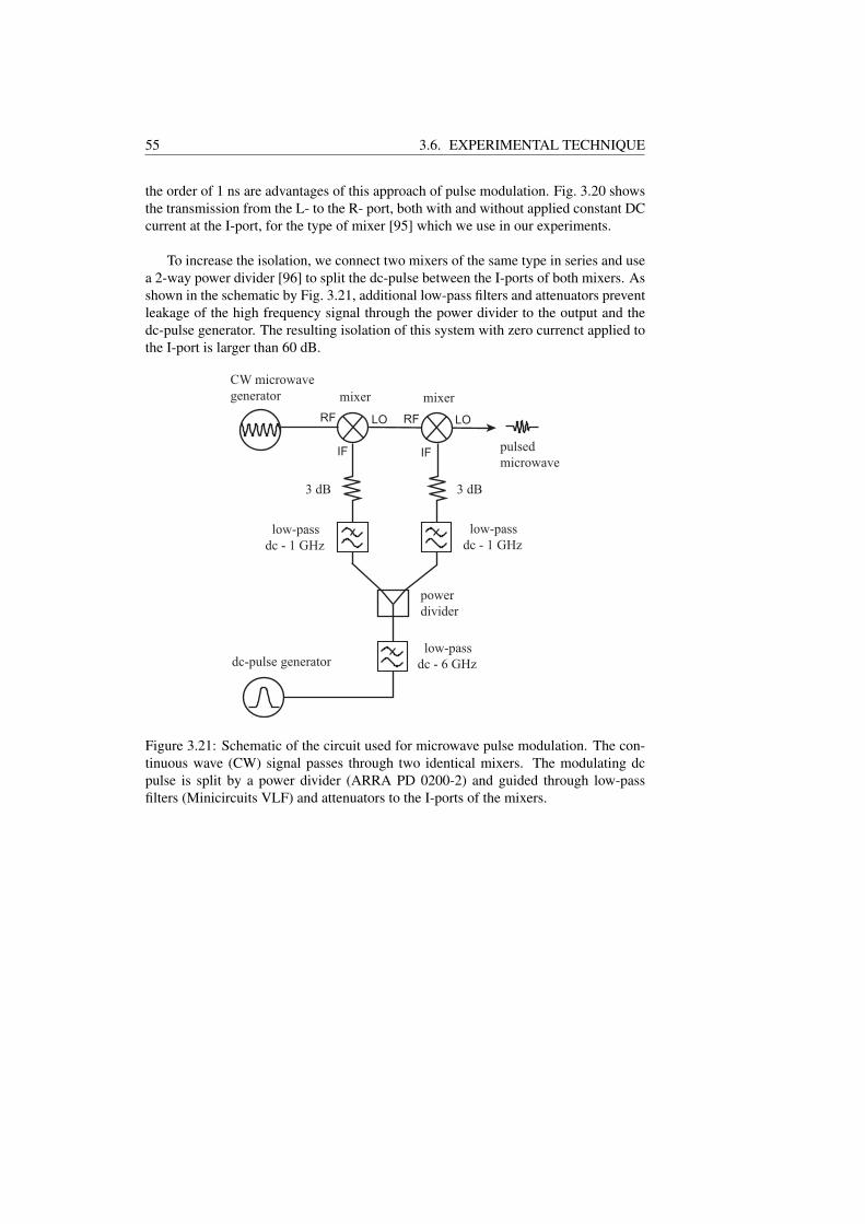
55 3.6. EXPERIMENTAL TECHNIQUE
the order of 1 ns are advantages of this approach of pulse modulation. Fig. 3.20 showsthe transmission from the L- to the R- port, both with and without applied constant DCcurrent at the I-port, for the type of mixer [95] which we use in our experiments.
To increase the isolation, we connect two mixers of the same type in series and usea 2-way power divider [96] to split the dc-pulse between the I-ports of both mixers. Asshown in the schematic by Fig. 3.21, additional low-pass filters and attenuators preventleakage of the high frequency signal through the power divider to the output and thedc-pulse generator. The resulting isolation of this system with zero currenct applied tothe I-port is larger than 60 dB.
CW microwave
generator mixer
power
divider
mixer
IFIF
LO LORFRF
pulsed
microwave
dc-pulse generator low-pass
dc - 6 GHz
3 dB3 dB
low-pass
dc - 1 GHz
low-pass
dc - 1 GHz
Figure 3.21: Schematic of the circuit used for microwave pulse modulation. The con-tinuous wave (CW) signal passes through two identical mixers. The modulating dcpulse is split by a power divider (ARRA PD 0200-2) and guided through low-passfilters (Minicircuits VLF) and attenuators to the I-ports of the mixers.

CHAPTER 3. THE FLUX-BIASED PHASE QUBIT 56

Chapter 4
Experimental results
4.1 Sample characterization
Once the sample has been cooled to milikelvin temperature, the dependence Isw(Φext)of the dc-SQUID switching current on external flux is acquired in a wide range tocharacterize the sample. Such a data set allows to estimate the critical currents and mu-tual inductances in the phase qubit system. Fig. 4.1 shows the result of an Isw(Φext)measurement for sample Hyp100, displaying the positions of histogram peaks in theswitching-current distribution. The horizontal scale on top of this figure has been re-calculated to display the flux Φsq in the dc-SQUID loop in units of Φ0, which is givenby the periodicity of the dc-SQUID critical current modulation.
The discrete steps appearing on the Isw(Φext) - pattern are the signature of thequbit undergoing transitions between wells at certain values of external flux. To makethe hysteresis between inter-well transitions visible, the external flux was swept intwo directions. As indicated in the figure, the periodicity at which these steps occurcorresponds to one flux quantum in the qubit loop. Renormalizing the horizontal axis tothe flux in the qubit loop Φq, as indicated by the bottom scale of Fig. 4.1, the parameterβL can be obtained from the measured hysteresis. As shown in Fig. 4.2, the hysteresisis linear for βL > 1 and exceeds one flux quantum above βL = 4.6. For the shown data,the hysteresis is estimated to be ≈ (1.39 ± 0.02) Φ0, resulting in βL ≈ 5.85 ± 0.09which is in accordance to the designed values as presented in Tab. 3.2.
The measurement of the βL value allows for a good estimation of the critical currentof the qubit junction, because the inductance L of the qubit loop depends only on itsgeometry. Loop inductances can therefore be precisely calculated with the aid of theFastHenry program up to an estimated uncertainty of 2.5 %. Likewise, the criticalcurrent of the dc-SQUID is measured from the modulation depth ∆I ′sq as shown inFig. 4.1, which depends on the βL,SQ - parameter [9]. From the shown data of sampleHyp100, we obtain βL,SQ ≈ 25±1, which corresponds to a dc-SQUID critical currentIc,sq ≈ (19.6± 0.8)µA.
The mutual inductance MqSq between qubit and dc-SQUID is estimated near aqubit step on a linear branch of the Isw(Φext) pattern as shown in the inset to Fig. 4.1.When the qubit switches between potential wells, the dc-SQUID switching currentchanges by a certain amount ∆Ic,sq. By comparing the value of external flux ∆Φ ′
sq
required to result in an equal change of ∆Ic,sq, the mutual inductance is calculatedas MqSq = ∆Φ ′
sq/∆Iq . The change in circulating current ∆Iq can be calculated
57
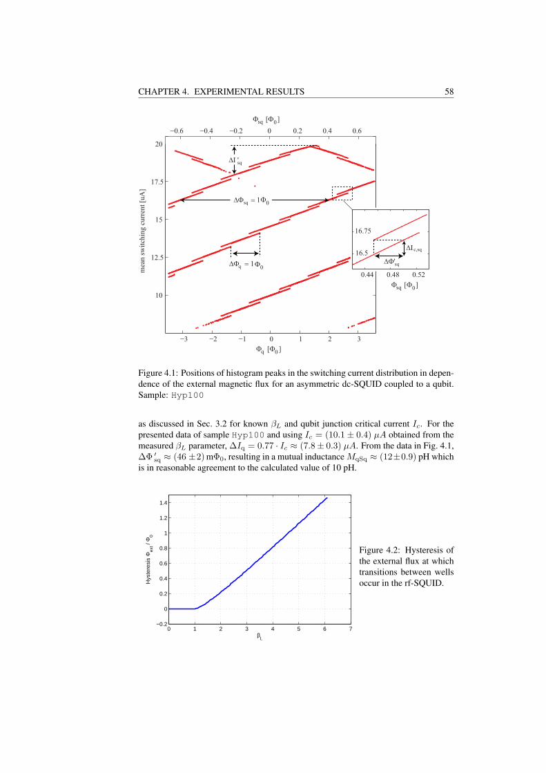
CHAPTER 4. EXPERIMENTAL RESULTS 58
−0.6 −0.4 −0.2 0 0.2 0.4 0.6
10
12.5
15
17.5
20
Φ [Φ ]
mea
n s
wit
chin
g c
urr
ent
[uA
]
0
−3 −2 −1 0 1 2 3
sq
Φ [Φ ]0q
0.44 0.48 0.52
16.5
16.75
∆Φ' sq
Φ [Φ ]0sq
∆Φ = 1 q Φ0
∆Φ = 1 sq Φ0
∆Ι ' sq
∆Ιc,sq
Figure 4.1: Positions of histogram peaks in the switching current distribution in depen-dence of the external magnetic flux for an asymmetric dc-SQUID coupled to a qubit.Sample: Hyp100
as discussed in Sec. 3.2 for known βL and qubit junction critical current Ic. For thepresented data of sample Hyp100 and using Ic = (10.1± 0.4) µA obtained from themeasured βL parameter, ∆Iq = 0.77 · Ic ≈ (7.8± 0.3) µA. From the data in Fig. 4.1,∆Φ ′
sq ≈ (46 ±2) mΦ0, resulting in a mutual inductance MqSq ≈ (12±0.9) pH whichis in reasonable agreement to the calculated value of 10 pH.
0 1 2 3 4 5 6 7−0.2
0
0.2
0.4
0.6
0.8
1
1.2
1.4
βL
Hys
tere
sis
Φex
t / Φ
0
Figure 4.2: Hysteresis ofthe external flux at whichtransitions between wellsoccur in the rf-SQUID.
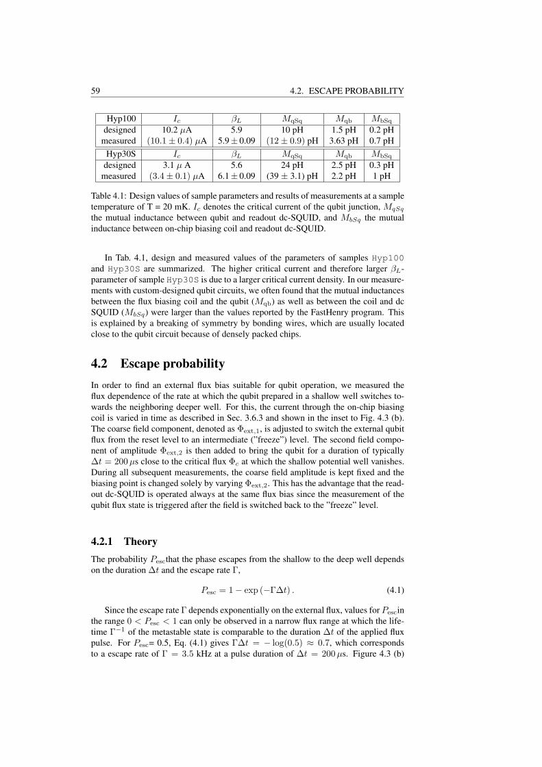
59 4.2. ESCAPE PROBABILITY
Hyp100 Ic βL MqSq Mqb MbSq
designed 10.2 µA 5.9 10 pH 1.5 pH 0.2 pHmeasured (10.1± 0.4) µA 5.9± 0.09 (12± 0.9) pH 3.63 pH 0.7 pH
Hyp30S Ic βL MqSq Mqb MbSq
designed 3.1 µ A 5.6 24 pH 2.5 pH 0.3 pHmeasured (3.4± 0.1) µA 6.1± 0.09 (39 ± 3.1) pH 2.2 pH 1 pH
Table 4.1: Design values of sample parameters and results of measurements at a sampletemperature of T = 20 mK. Ic denotes the critical current of the qubit junction, MqSq
the mutual inductance between qubit and readout dc-SQUID, and MbSq the mutualinductance between on-chip biasing coil and readout dc-SQUID.
In Tab. 4.1, design and measured values of the parameters of samples Hyp100and Hyp30S are summarized. The higher critical current and therefore larger βL-parameter of sample Hyp30S is due to a larger critical current density. In our measure-ments with custom-designed qubit circuits, we often found that the mutual inductancesbetween the flux biasing coil and the qubit (Mqb) as well as between the coil and dcSQUID (MbSq) were larger than the values reported by the FastHenry program. Thisis explained by a breaking of symmetry by bonding wires, which are usually locatedclose to the qubit circuit because of densely packed chips.
4.2 Escape probabilityIn order to find an external flux bias suitable for qubit operation, we measured theflux dependence of the rate at which the qubit prepared in a shallow well switches to-wards the neighboring deeper well. For this, the current through the on-chip biasingcoil is varied in time as described in Sec. 3.6.3 and shown in the inset to Fig. 4.3 (b).The coarse field component, denoted as Φext,1, is adjusted to switch the external qubitflux from the reset level to an intermediate (”freeze”) level. The second field compo-nent of amplitude Φext,2 is then added to bring the qubit for a duration of typically∆t = 200 µs close to the critical flux Φc at which the shallow potential well vanishes.During all subsequent measurements, the coarse field amplitude is kept fixed and thebiasing point is changed solely by varying Φext,2. This has the advantage that the read-out dc-SQUID is operated always at the same flux bias since the measurement of thequbit flux state is triggered after the field is switched back to the ”freeze” level.
4.2.1 TheoryThe probability Pescthat the phase escapes from the shallow to the deep well dependson the duration ∆t and the escape rate Γ,
Pesc = 1− exp (−Γ∆t) . (4.1)
Since the escape rate Γ depends exponentially on the external flux, values for Pescinthe range 0 < Pesc < 1 can only be observed in a narrow flux range at which the life-time Γ−1 of the metastable state is comparable to the duration ∆t of the applied fluxpulse. For Pesc= 0.5, Eq. (4.1) gives Γ∆t = − log(0.5) ≈ 0.7, which correspondsto a escape rate of Γ = 3.5 kHz at a pulse duration of ∆t = 200 µs. Figure 4.3 (b)
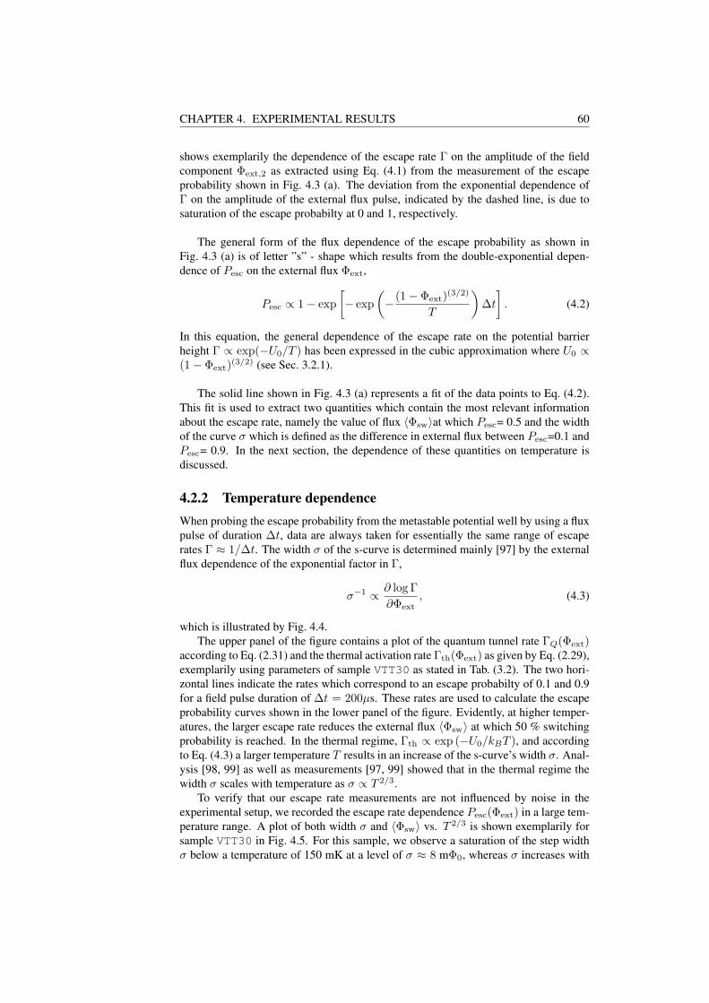
CHAPTER 4. EXPERIMENTAL RESULTS 60
shows exemplarily the dependence of the escape rate Γ on the amplitude of the fieldcomponent Φext,2 as extracted using Eq. (4.1) from the measurement of the escapeprobability shown in Fig. 4.3 (a). The deviation from the exponential dependence ofΓ on the amplitude of the external flux pulse, indicated by the dashed line, is due tosaturation of the escape probabilty at 0 and 1, respectively.
The general form of the flux dependence of the escape probability as shown inFig. 4.3 (a) is of letter ”s” - shape which results from the double-exponential depen-dence of Pesc on the external flux Φext,
Pesc ∝ 1− exp[− exp
(− (1− Φext)(3/2)
T
)∆t
]. (4.2)
In this equation, the general dependence of the escape rate on the potential barrierheight Γ ∝ exp(−U0/T ) has been expressed in the cubic approximation where U0 ∝(1− Φext)(3/2) (see Sec. 3.2.1).
The solid line shown in Fig. 4.3 (a) represents a fit of the data points to Eq. (4.2).This fit is used to extract two quantities which contain the most relevant informationabout the escape rate, namely the value of flux 〈Φsw〉at which Pesc= 0.5 and the widthof the curve σ which is defined as the difference in external flux between Pesc=0.1 andPesc= 0.9. In the next section, the dependence of these quantities on temperature isdiscussed.
4.2.2 Temperature dependenceWhen probing the escape probability from the metastable potential well by using a fluxpulse of duration ∆t, data are always taken for essentially the same range of escaperates Γ ≈ 1/∆t. The width σ of the s-curve is determined mainly [97] by the externalflux dependence of the exponential factor in Γ,
σ−1 ∝ ∂ log Γ∂Φext
, (4.3)
which is illustrated by Fig. 4.4.The upper panel of the figure contains a plot of the quantum tunnel rate ΓQ(Φext)
according to Eq. (2.31) and the thermal activation rate Γth(Φext) as given by Eq. (2.29),exemplarily using parameters of sample VTT30 as stated in Tab. (3.2). The two hori-zontal lines indicate the rates which correspond to an escape probabilty of 0.1 and 0.9for a field pulse duration of ∆t = 200µs. These rates are used to calculate the escapeprobability curves shown in the lower panel of the figure. Evidently, at higher temper-atures, the larger escape rate reduces the external flux 〈Φsw〉 at which 50 % switchingprobability is reached. In the thermal regime, Γth ∝ exp (−U0/kBT ), and accordingto Eq. (4.3) a larger temperature T results in an increase of the s-curve’s width σ. Anal-ysis [98, 99] as well as measurements [97, 99] showed that in the thermal regime thewidth σ scales with temperature as σ ∝ T 2/3.
To verify that our escape rate measurements are not influenced by noise in theexperimental setup, we recorded the escape rate dependence Pesc(Φext) in a large tem-perature range. A plot of both width σ and 〈Φsw〉 vs. T 2/3 is shown exemplarily forsample VTT30 in Fig. 4.5. For this sample, we observe a saturation of the step widthσ below a temperature of 150 mK at a level of σ ≈ 8 mΦ0, whereas σ increases with

61 4.2. ESCAPE PROBABILITY
2.1 2.2 2.3 2.4 2.5 2.6 2.7
0.1
0.5
0. 9
1
10
102
103
104
105
esca
pe
Rat
e [s
]es
cap
e p
rob
abil
ity
P
esc
1
-1
0
σ
Φext,2
Φext,1
∆t
Φ [a.u.]ext 2
(a)
(b)
<Φ >sw
Figure 4.3: (a) Escape probability vs. the amplitude of an external flux pulse Φext,2 of∆t = 200µs duration, measured on sample VTT30. (b) Escape rate calculated fromthe data shown in (a). Inset: timing profile of the external flux, which is composedfrom two pulses of amplitudes Φext,1 and Φext,2, respectively. Both field componentshave a rise time of ≈ 20µs.
temperature as expected proportionally to T 2/3 up to ≈ 22 mΦ0 at T = 800 mK. Thesolid lines drawn in Fig. 4.5 are extracted from numerically calculated s-curves usingthe sum of thermal and quantum escape rates Γth(T ) + ΓQ. Calculation of these lineswas done by using the design values of sample VTT30 as stated in Tab. (3.2) and fit-ting the junction capacitance, resulting in C = 0.2 pF. In Fig. 4.5 (b), the data pointswere shifted (but not scaled) along the vertical flux axis to make them coincide with thecalculated external flux at the lowest temperature. This is justified because the criticalflux Φc is per se not a measurable quantity [100].
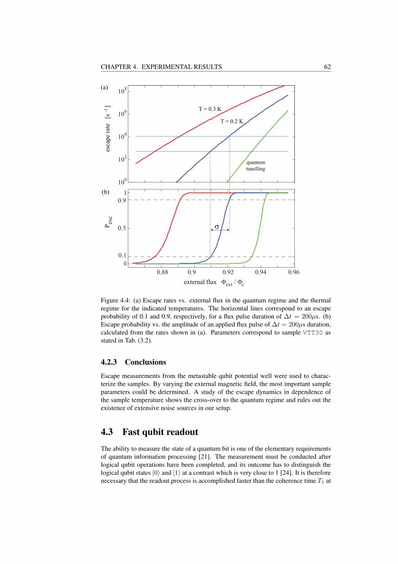
CHAPTER 4. EXPERIMENTAL RESULTS 62
100
102
104
106
108
0.88 0.9 0.92 0.94 0.96
0
0.1
0.5
0.9
1
Pes
ces
cap
e ra
te
[s
]
-1 T = 0.3 K
T = 0.2 K
quantum
tunelling
σ
Φ / Φext cexternal flux
(a)
(b)
Figure 4.4: (a) Escape rates vs. external flux in the quantum regime and the thermalregime for the indicated temperatures. The horizontal lines correspond to an escapeprobability of 0.1 and 0.9, respectively, for a flux pulse duration of ∆t = 200µs. (b)Escape probability vs. the amplitude of an applied flux pulse of ∆t = 200µs duration,calculated from the rates shown in (a). Parameters correspond to sample VTT30 asstated in Tab. (3.2).
4.2.3 Conclusions
Escape measurements from the metastable qubit potential well were used to charac-terize the samples. By varying the external magnetic field, the most important sampleparameters could be determined. A study of the escape dynamics in dependence ofthe sample temperature shows the cross-over to the quantum regime and rules out theexistence of extensive noise sources in our setup.
4.3 Fast qubit readout
The ability to measure the state of a quantum bit is one of the elementary requirementsof quantum information processing [21]. The measurement must be conducted afterlogical qubit operations have been completed, and its outcome has to distinguish thelogical qubit states |0〉 and |1〉 at a contrast which is very close to 1 [24]. It is thereforenecessary that the readout process is accomplished faster than the coherence time T1 at

63 4.3. FAST QUBIT READOUT
6
10
14
18
22
0 0.1 0.2 0.3 0.4 0.5 0.6 0.7 0.8 0.9
wid
th
[ mΦ
0]
Temperature [K ]
50
% P
osi
tio
n [
rel.
]Φ
02/32/3
0.82
0.86
0.9
0.94
σ
0.1 0.2 0.3 0.4 0.5 0.60.02 0.80.7
Temperature [K]
(a)
(b)
Figure 4.5: Temperature dependence of the inter-well transition, measured on sampleVTT30. (a) width of the qubit step in units of the flux quantum Φ0. (b) externalflux at which the escape probability is equal to 50 %. Data points in (b) were shiftedto meet the calculated position at the lowest temperature. Solid lines in both panelswere calculated numerically leaving the junction capacitance as the only free fittingparameter. Indicated by the arrow is the temperature ≈ 150 mK above which thermalescape occurs.
which depolarization of the qubit states occurs.
4.3.1 Theory
For superconducting phase qubits, a measurement technique has been implementedwhich complies with above requirements [34, 35, 36]. Its principle is to shortly reducethe potential barrier of the well which contains the qubit states to allow the excited stateof higher energy to tunnel into a macroscopically distinguishable state. The groundstate remains in the initial well in this readout procedure.
In flux-biased phase qubits, this is accomplished by applying a dc-pulse of fluxwhich increases the total flux in the qubit loop. Its effect is to provide an additional tiltin the qubit potential as shown in Fig. 4.6 (a), increasing the escape rate towards theneighboring potential well for all states which are contained in the shallow potentialwell. However, since the escape rate of the excited state is typically a factor of 102
- 103 higher than the one of the ground state, it is possible to adjust the duration andamplitude of the flux pulse such that during its application only the excited state escapesat large probability.

CHAPTER 4. EXPERIMENTAL RESULTS 64
60 70 80 90
0
0.2
0.4
0.6
0.8
1
1 0Γ1
(a) (b)
mΦ /Φcdc
ϕ
U
P esc
Figure 4.6: (a) Illustration of the effect of the readout dc-pulse on the qubit potential.Dashed lines show the potential well before the dc-pulse was applied, solid lines thepotential during the readout pulse. (b) The calculated escape probability for a qubitprepared in states |0〉 and |1〉, read out by a gaussian readout pulse of duration Wdc
= 2 ns and amplitude Φdc. Also shown by the red solid line is the readout contrastas the difference between the two curves. The dashed lines are calculated by takinginto account energy relaxation during the readout at a T1 - time of 1 ns, resulting in amaximum readout contrast of 0.93. Calculations were done using parameters of sampleVTT30.
Figure 4.6 (b) illustrates the increase of the escape probability Pescwith the ampli-tude Φdc of a readout flux pulse for the two cases when the qubit was prepared in eitherthe ground or excited state. For these calculations, a gaussian-shaped readout dc-pulsecreates the time-dependent external flux
Φext(t) = Φs + Φdc · exp[− (t− w)2
2 w2
]. (4.4)
Here, Φs is the starting value of bias flux (at which qubit operations are done), Φdc isthe amplitude of the gaussian flux pulse and w is its width which is related to the fullwidth at half maximum Wdc by w = Wdc/(2
√2 log 2). The escape probability was
then obtained by numerical integration of the equation
Pesc = 1− exp(−
∫Γ(t)dt
), (4.5)
where Γ(t) = p0Γ0(t)+ p1Γ1(t) is the sum of the escape rates of the two states whosepopulation probabilities are p0 = 1 − p1 and p1, respectively. This rate is calculatedfrom the WKB-result for quantum tunneling Eq. (2.31) and depends on time accordingto the time-varying external flux Eq. (4.4).
We define the fidelity of the readout as the difference between the obtained escapeprobabilities of the excited state and the ground state. Figure 4.6 (b), which was cal-culated using parameters of sample VTT30 and a readout pulse duration Wdc = 2 ns,shows that the maximal contrast of 0.99 is very close to 100 % since the curves for thetwo states are well separated. The decay of the excited state due to energy relaxation

65 4.3. FAST QUBIT READOUT
during the readout pulse was taken into account by correcting the excited state popula-tion by the factor exp(−t/T1), where T1 is the lifetime of state |1〉. The result of sucha calculation, using T1 = 1 ns, is shown by the dashed lines in Fig. 4.6 (b), reaching amaximal readout fidelity of 93%.
4.3.2 Sources of readout errors
In a real experiment, several mechanisms contribute to a reduction of the attainablereadout fidelity, of which the most prominent are those related to a change of the levelpopulation during the readout process. This can be due to energy relaxation, which isavoidable by using very short and fast rising readout pulses. However, when a shortpulse is to be used, its amplitude must be made large enough to reach flux values atwhich the excited state tunnels in a time which is comparable to the readout pulseduration. The readout hence occurs close to the critical flux where the ratio Γ1/Γ0 de-creases as it is shown in Fig. 3.6, and therefore also the measurement fidelity decreases.
A short readout pulse may furthermore act non-adiabatically and alter the statepopulations when its fourier components are resonant to transitions to upper levels.Analysis [68] has shown that for typical phase qubits (having transition frequenciesω10/2π ≈ 10 GHz) the probability of nonadiabatic excitation is of order 10−2 forlinear readout pulses of 500 ps rise times but is further reduced to below 10−4 forgaussian-shaped pulses.
During application of the readout pulse, the qubit resonance frequency is continu-ously reduced and may be changed by a factor of up to 1/2. If there exists a parasiticresonator [27] below the qubit working frequency, the readout pulse may sweep thequbit through their common resonance. Given that it is coupled sufficiently strong, thecoherent oscillations in the resulting four-state system may be fast enough to changethe qubit state [34]. Lastly, for flux-biased phase qubits, a measurement error due toresonant tunneling, which occurs when the states in the left well and the deep right wellalign, has been considered [68]. While this mechanism may in principle give rise to arepopulation of the shallow well once tunneling to the deep well occurred, the stronglyincreased energy relaxation rate from highly excited states in the deep well renders thispossibility unlikely.
4.3.3 Experimental results
Similar to above described calculations, the readout fidelity has been probed exper-imentally by recording the escape probability curves versus the amplitude of an ap-plied dc-flux pulse. The result, obtained from sample VTT30, is shown in Fig. 4.7for three different readout pulse widths. The excited state was populated by a reso-nant microwave π-pulse whose duration was 1.2 ns as found by observing coherentoscillations at the same bias parameters. The largest readout fidelity of 78.3 % wasobtained for the shortest dc-pulse of 1 ns width, while for the longest pulse of duration5 ns the fidelity decreased to 19.6 % due to significant energy relaxation during thereadout. Since for this sample the time Td, which is the half-lifetime during which theamplitude of driven coherent oscillation decays to 1/e, is about 4 ns, decoherence oc-curs already during the populating microwave pulse. This can explain the significantlyreduced maximum readout contrast. During a microwave pulse of duration Tµw, bothstates approach 50% population due to decoherence resulting in a finally equal rate of
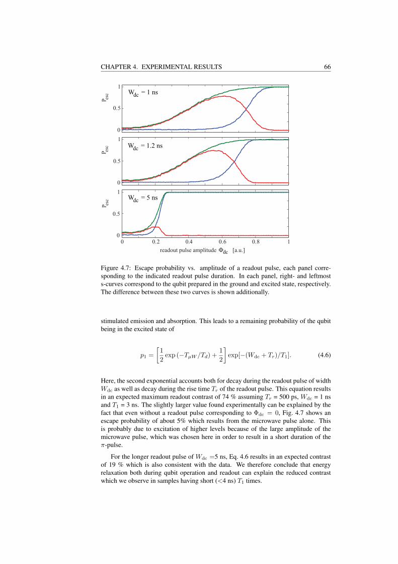
CHAPTER 4. EXPERIMENTAL RESULTS 66
0
0.5
1
0
0.5
1
0 0.2 0.4 0.6 0.8 1
readout pulse amplitude [a.u.]
P esc
0
0.5
1
P esc
P esc
Φ dc
W = 1 nsdc
W = 1.2 nsdc
W = 5 nsdc
Figure 4.7: Escape probability vs. amplitude of a readout pulse, each panel corre-sponding to the indicated readout pulse duration. In each panel, right- and leftmosts-curves correspond to the qubit prepared in the ground and excited state, respectively.The difference between these two curves is shown additionally.
stimulated emission and absorption. This leads to a remaining probability of the qubitbeing in the excited state of
p1 =[12
exp (−TµW /Td) +12
]exp[−(Wdc + Tr)/T1]. (4.6)
Here, the second exponential accounts both for decay during the readout pulse of widthWdc as well as decay during the rise time Tr of the readout pulse. This equation resultsin an expected maximum readout contrast of 74 % assuming Tr = 500 ps, Wdc = 1 nsand T1 = 3 ns. The slightly larger value found experimentally can be explained by thefact that even without a readout pulse corresponding to Φdc = 0, Fig. 4.7 shows anescape probability of about 5% which results from the microwave pulse alone. Thisis probably due to excitation of higher levels because of the large amplitude of themicrowave pulse, which was chosen here in order to result in a short duration of theπ-pulse.
For the longer readout pulse of Wdc =5 ns, Eq. 4.6 results in an expected contrastof 19 % which is also consistent with the data. We therefore conclude that energyrelaxation both during qubit operation and readout can explain the reduced contrastwhich we observe in samples having short (<4 ns) T1 times.
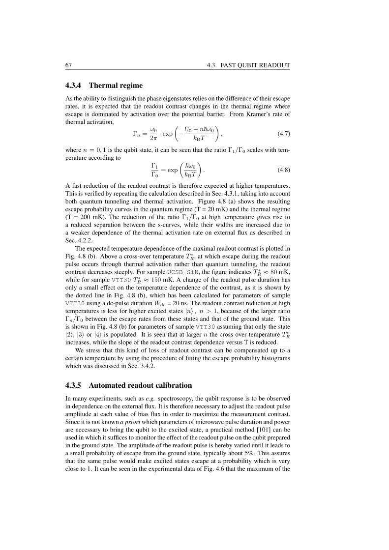
67 4.3. FAST QUBIT READOUT
4.3.4 Thermal regimeAs the ability to distinguish the phase eigenstates relies on the difference of their escaperates, it is expected that the readout contrast changes in the thermal regime whereescape is dominated by activation over the potential barrier. From Kramer’s rate ofthermal activation,
Γn =ω0
2π· exp
(−U0 − n~ω0
kBT
), (4.7)
where n = 0, 1 is the qubit state, it can be seen that the ratio Γ1/Γ0 scales with tem-perature according to
Γ1
Γ0= exp
(~ω0
kBT
). (4.8)
A fast reduction of the readout contrast is therefore expected at higher temperatures.This is verified by repeating the calculation described in Sec. 4.3.1, taking into accountboth quantum tunneling and thermal activation. Figure 4.8 (a) shows the resultingescape probability curves in the quantum regime (T = 20 mK) and the thermal regime(T = 200 mK). The reduction of the ratio Γ1/Γ0 at high temperature gives rise toa reduced separation between the s-curves, while their widths are increased due toa weaker dependence of the thermal activation rate on external flux as described inSec. 4.2.2.
The expected temperature dependence of the maximal readout contrast is plotted inFig. 4.8 (b). Above a cross-over temperature T ∗R, at which escape during the readoutpulse occurs through thermal activation rather than quantum tunneling, the readoutcontrast decreases steeply. For sample UCSB-SiN, the figure indicates T ∗R ≈ 80 mK,while for sample VTT30 T ∗R ≈ 150 mK. A change of the readout pulse duration hasonly a small effect on the temperature dependence of the contrast, as it is shown bythe dotted line in Fig. 4.8 (b), which has been calculated for parameters of sampleVTT30 using a dc-pulse duration Wdc = 20 ns. The readout contrast reduction at hightemperatures is less for higher excited states |n〉 , n > 1, because of the larger ratioΓn/Γ0 between the escape rates from these states and that of the ground state. Thisis shown in Fig. 4.8 (b) for parameters of sample VTT30 assuming that only the state|2〉, |3〉 or |4〉 is populated. It is seen that at larger n the cross-over temperature T ∗Rincreases, while the slope of the readout contrast dependence versus T is reduced.
We stress that this kind of loss of readout contrast can be compensated up to acertain temperature by using the procedure of fitting the escape probability histogramswhich was discussed in Sec. 3.4.2.
4.3.5 Automated readout calibrationIn many experiments, such as e.g. spectroscopy, the qubit response is to be observedin dependence on the external flux. It is therefore necessary to adjust the readout pulseamplitude at each value of bias flux in order to maximize the measurement contrast.Since it is not known a priori which parameters of microwave pulse duration and powerare necessary to bring the qubit to the excited state, a practical method [101] can beused in which it suffices to monitor the effect of the readout pulse on the qubit preparedin the ground state. The amplitude of the readout pulse is hereby varied until it leads toa small probability of escape from the ground state, typically about 5%. This assuresthat the same pulse would make excited states escape at a probability which is veryclose to 1. It can be seen in the experimental data of Fig. 4.6 that the maximum of the

CHAPTER 4. EXPERIMENTAL RESULTS 68
40 50 60 70 80
0
0.2
0.4
0.6
0.8
1
0 0.2 0.4 0.6 0.8 1
0
0.2
0.4
0.6
0.8
1
40 50 60 70 80
1 0
1 0
mΦ /Φcdc
read
ou
t co
ntr
ast
P esc
(a)T = 0.02 K T = 0.2 K
(b)
temperature [K]
mΦ /Φcdc
W = 20 nsdc
UCSB-SiN,
W = 20 nsdc
VTT, 1
VTT, 2
VTT, 3
W = 2 nsdc
VTT, 4
Figure 4.8: (a) Escape probability Pesc vs. readout pulse amplitude Φdc at T = 20 mK(left panel) and T = 200 mK (right panel), for the qubit prepared in state |0〉 and |1〉.The readout contrast is given by the maximal difference between the two curves. (b)Maximum of the readout contrast vs. temperature. Dashed line: sample UCSB-SiN,readout pulse duration Wdc = 20 ns. Other lines: sample VTT30, readout pulse du-ration Wdc = 2 ns, except dotted line: Wdc = 20 ns. The Ket-vector indicates whichexcited state is populated by 100%.
readout contrast is indeed found at readout pulse amplitudes which result in a smallescape probability from the ground state.
For automated readout calibration we implemented a function in the measurementsoftware which finds a suitable amplitude using the binary search algorithm. It beginsby measuring the reference escape probability Pref when the readout pulse is switchedoff. The pulse amplitude is then varied, after each change recording the escape proba-bility from a set of 500 samples. The algorithm stops when the guessed readout pulseamplitude results in an escape probability which is in the range of 4 to 8 % larger thanPref , which usually requires less than 10 iterations. Calibration values are then storedin a table which is used for subsequent experiments.
Figure 4.9 shows that the automatically calibrated readout pulse amplitude dependslinearly on the external flux, as expected. It is therefore sufficient to run the calibrationprocedure at a few flux values within the range of the experiment and use the results of
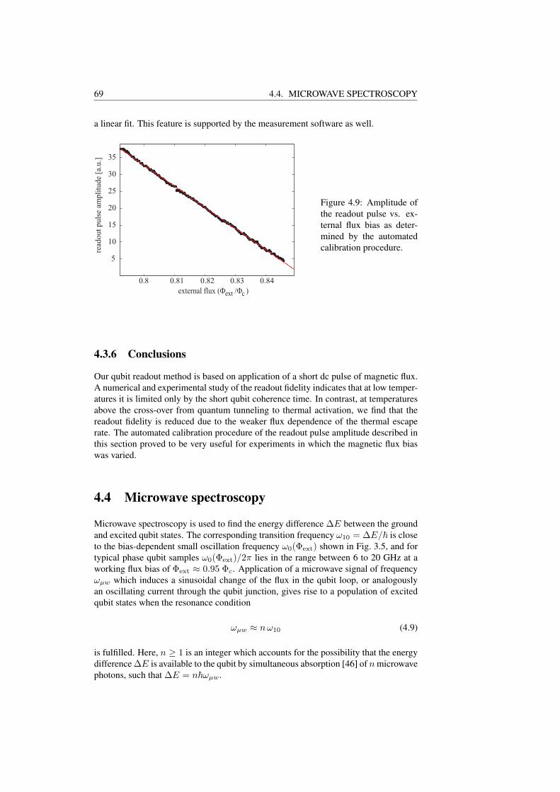
69 4.4. MICROWAVE SPECTROSCOPY
a linear fit. This feature is supported by the measurement software as well.
0.8 0.81 0.82 0.83 0.84
5
10
15
20
25
30
35
external flux (Φ /Φ )cext
read
out
pu
lse
ampli
tud
e [a
.u.]
Figure 4.9: Amplitude ofthe readout pulse vs. ex-ternal flux bias as deter-mined by the automatedcalibration procedure.
4.3.6 Conclusions
Our qubit readout method is based on application of a short dc pulse of magnetic flux.A numerical and experimental study of the readout fidelity indicates that at low temper-atures it is limited only by the short qubit coherence time. In contrast, at temperaturesabove the cross-over from quantum tunneling to thermal activation, we find that thereadout fidelity is reduced due to the weaker flux dependence of the thermal escaperate. The automated calibration procedure of the readout pulse amplitude described inthis section proved to be very useful for experiments in which the magnetic flux biaswas varied.
4.4 Microwave spectroscopy
Microwave spectroscopy is used to find the energy difference ∆E between the groundand excited qubit states. The corresponding transition frequency ω10 = ∆E/~ is closeto the bias-dependent small oscillation frequency ω0(Φext) shown in Fig. 3.5, and fortypical phase qubit samples ω0(Φext)/2π lies in the range between 6 to 20 GHz at aworking flux bias of Φext ≈ 0.95 Φc. Application of a microwave signal of frequencyωµw which induces a sinusoidal change of the flux in the qubit loop, or analogouslyan oscillating current through the qubit junction, gives rise to a population of excitedqubit states when the resonance condition
ωµw ≈ nω10 (4.9)
is fulfilled. Here, n ≥ 1 is an integer which accounts for the possibility that the energydifference ∆E is available to the qubit by simultaneous absorption [46] of n microwavephotons, such that ∆E = n~ωµw.
CHAPTER 4. EXPERIMENTAL RESULTS 70
4.4.1 The resonantly driven spin-12
system
The dynamics of the resonantly driven spin- 12 system are described by the Bloch equa-
tions [102]
d〈σx(t)〉dt
=[γ〈σ(t)〉 × ~B(t)
]x− 〈σy(t)〉
T2(4.10)
d〈σy(t)〉dt
=[γ〈σ(t)〉 × ~B(t)
]y− 〈σy(t)〉
T2(4.11)
d〈σz(t)〉dt
=[γ〈σ(t)〉 × ~B(t)
]z− 〈σz(t)〉 − σ0
T1, (4.12)
which characterize the time evolution of the spin σ with gyromagnetic ratio γ in thetime-dependent magnetic field
~B(t) = Bx(t), By(t), Bz. (4.13)
These equations contain the energy relaxation time T1 and the phase coherence timeT2 as well as the thermally-induced population of the excited state σ0 = tanh (∆E/kBT ).The static longitudinal field component Bz is related to the Larmor frequency
ω10 = ∆E/~ = γBz, (4.14)
at which the spin precesses around the z-axis. For phase qubits, the Larmor frequencyis determined by the energy difference between the qubit states ∆E. The Bloch equa-tions can be solved analytically when the time-dependent transversal field rotates at theLarmor frequency around the z-axis, so that it follows the precessing spin:
Bx(t) = Bt cos(ω10t); By(t) = Bt sin(ω10t). (4.15)
In a frame rotating at the Larmor frequency, this results in an effective constant transver-sal field. Since the phase qubit is merely a pseudo-spin, it is not possible to apply arotating transversal field, but only a sinusoidal drive which has transversal as well aslongitudinal components. However, the longitudinal component, which modulates theLarmor frequency, can be neglected in practical experiments where the Rabi frequencyat which the spin rotates around the x-axis is much smaller than the precession fre-quency [103].
Experimentally, spectroscopy is done by using a microwave pulse of duration τµw >T1 to ensure that eventual coherent oscillation in the state population decay towards aconstant probability of remaining in the excited state. This corresponds to a steady statedσ/dt = 0. Immediately after the microwave pulse, the readout dc-pulse is applied toprobe the qubit state, hereby realizing a measurement of the z-component 〈σz〉. Ameasurement of the escape probability in dependence of microwave frequency or ex-ternal flux bias then displays a resonance curve which has the form of a Lorentziangiven by [104]
〈σz〉 =
1− ω2
R T1T2
1 +(
ω10−ωµwT2
)2
+ ω2R T1T2
σ0. (4.16)
Here, ωR ∝ Jn(α) is the Rabi frequency, which is for a n-photon process proportionalto the nth order Bessel function of the first kind Jn(α) of the normalized amplitude of

71 4.4. MICROWAVE SPECTROSCOPY
the driving field α ∝ Bx for By = 0. [105]. For the one-photon process, ωR scaleslinearly with α as long as ωR ¿ ω10.
From Eq. (4.16) it follows that the full width at half maximum of the resonancecurve is
σ =2T2
√1 + ω2
R T1 T2 (4.17)
and the amplitude of the resonance is
A =ω2
R T1 T2
1 + ω2R T1 T2
σ0. (4.18)
4.4.2 Spectroscopy at small drive amplitude
0.92 0.94 0.96 0.98
0
2
4
6
8
0
0.1
0.2
esca
pe
pro
bab
ilty
P esc
6.3 GHz7 GHz
7.5 GHz
8 GHz
external flux (Φ /Φ )cext
mic
row
ave
freq
uen
cy [
GH
z]
Figure 4.10: Top panel: The applied microwave frequency plotted vs. the value ofexternal flux at which the resonance peak is found. Solid line is a fit to the smalloscillation frequency ω0/2π, resulting in Ic = 1.65µA and C = 832 fF for a fixedinductance L = 720 pH. Bottom panel: Resonance peaks in the escape probability,obtained by varying the external flux. Solid lines are fits to Lorentz curves. The shownresonance curves have Q-factors of ≈ 100, which are limited by the drive amplitude.Data has been taken using sample UCSB-SiN.
Resonance curves obtained from sample UCSB-SiN are plotted in the bottompanel of Fig. 4.10, using a microwave pulse of 200 ns duration at the frequencies in-dicated in the figure. The value of external flux at which these resonances are located

CHAPTER 4. EXPERIMENTAL RESULTS 72
depends on the chosen microwave frequency as shown in the top panel of Fig. 4.10.Here, the solid line is obtained from a fit of the resonance positions to a numericalcalculation of the small oscillation frequency ω0, using the junction critical current andcapacitance as free parameters. However, this data does not allow to determine thesample parameters exactly, since the externally applied flux is known only up to anadditive constant. This third fitting parameter is therefore required which is not inde-pendent of the qubit parameters.
4.4.3 Parasitic resonances the setup
Our attainable resolution of microwave spectroscopy is limited by the parasitic reso-nances in our experimental setup. These give rise to a frequency modulation of themicrowave power that couples to the qubit, hereby changing the amplitude and widthof the resonance peak. Figure 4.11 shows exemplarily the result of spectroscopy per-formed on sample HYP100 using a fixed microwave power. The strong oscillation inthe width of the trace is due to harmonics of a parasitic resonance of about 300 MHz.At frequencies where much power couples to the qubit, we observe a second peakwhich is due to a higher-order transition as described in the next section. In principle,it is possible to avoid this effect by adjusting the microwave power at each frequencyto the frequency-dependent coupling coefficient between source and qubit, which canbe evaluated from the amplitude of the resonance peak using Eq. (4.18).
0.94 0.945 0.95 0.955
external flux Φ / Φcext
25
24
23
24.5
23.5
22.5
0.4
0.3
0.2
0.1
Pesc
mic
row
ave
freq
uen
cy
Figure 4.11: Spectroscopy on sample Hyp100.
Parasitic resonances can also be visualized in situ by measuring the frequency de-pendence of the power that is required to induce an off-resonant escape from a veryshallow potential well as shown in Fig. 4.12. This data was acquired without using areadout pulse by biasing the qubit close the critical flux where the escape probabilityfrom the ground state was about 20%. An automated program varied the microwave
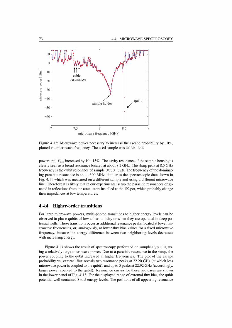
73 4.4. MICROWAVE SPECTROSCOPY
7 7.5 8 8.5 9
−60
−50
−40
−30
−20
−10
0
10
microwave frequency [GHz]
mic
row
ave
pow
er [
dB
m]
sample holderqubit
cableresonances
Figure 4.12: Microwave power necessary to increase the escape probability by 10%,plotted vs. microwave frequency. The used sample was UCSB-SiN.
power until Pesc increased by 10 - 15%. The cavity resonance of the sample housing isclearly seen as a broad resonance located at about 8.2 GHz. The sharp peak at 8.5 GHzfrequency is the qubit resonance of sample UCSB-SiN. The frequency of the dominat-ing parasitic resonance is about 300 MHz, similar to the spectroscopic data shown inFig. 4.11 which was measured on a different sample and using a different microwaveline. Therefore it is likely that in our experimental setup the parasitic resonances origi-nated in reflections from the attenuators installed at the 1K-pot, which probably changetheir impedances at low temperatures.
4.4.4 Higher-order transitions
For large microwave powers, multi-photon transitions to higher energy levels can beobserved in phase qubits of low anharmonicity or when they are operated in deep po-tential wells. These transitions occur as additional resonance peaks located at lower mi-crowave frequencies, or, analogously, at lower flux bias values for a fixed microwavefrequency, because the energy difference between two neighboring levels decreaseswith increasing energy.
Figure 4.13 shows the result of spectroscopy performed on sample Hyp100, us-ing a relatively large microwave power. Due to a parasitic resonance in the setup, thepower coupling to the qubit increased at higher frequencies. The plot of the escapeprobability vs. external flux reveals two resonance peaks at 22.20 GHz (at which lessmicrowave power is coupled to the qubit), and up to 5 peaks at 22.92 GHz (accordingly,larger power coupled to the qubit). Resonance curves for these two cases are shownin the lower panel of Fig. 4.13. For the displayed range of external flux bias, the qubitpotential well contained 8 to 5 energy levels. The positions of all appearing resonance
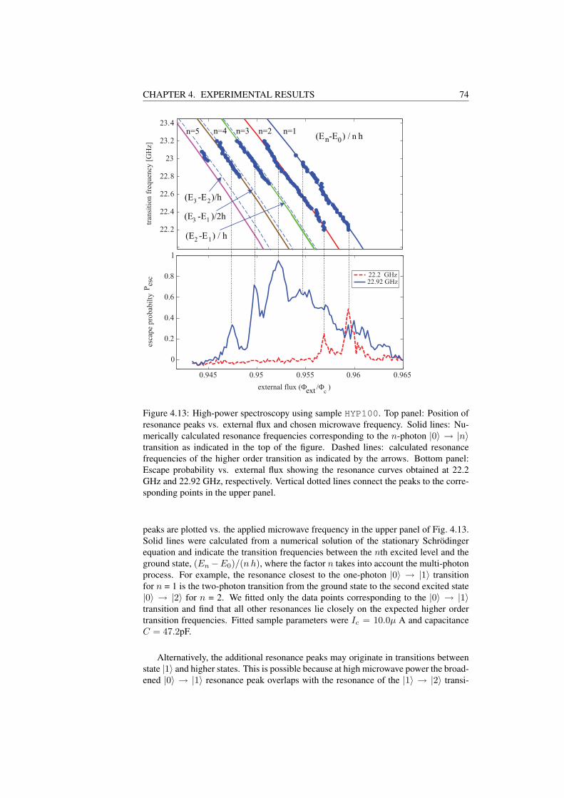
CHAPTER 4. EXPERIMENTAL RESULTS 74
0.945 0.95 0.955 0.96 0.965
22.2
22.4
22.6
22.8
23
23.2
23.4
tran
siti
on f
requen
cy [
GH
z]
0
0.2
0.4
0.6
0.8
1
esca
pe
pro
bab
ilty
Pes
c 22.2 GHz22.92 GHz
external flux (Φ /Φ )cext
(E -E ) / n hn 0
n=1n=2n=3n=4n=5
(E -E )/h3 2
(E -E )/2h3 1
(E -E ) / h2 1
Figure 4.13: High-power spectroscopy using sample HYP100. Top panel: Position ofresonance peaks vs. external flux and chosen microwave frequency. Solid lines: Nu-merically calculated resonance frequencies corresponding to the n-photon |0〉 → |n〉transition as indicated in the top of the figure. Dashed lines: calculated resonancefrequencies of the higher order transition as indicated by the arrows. Bottom panel:Escape probability vs. external flux showing the resonance curves obtained at 22.2GHz and 22.92 GHz, respectively. Vertical dotted lines connect the peaks to the corre-sponding points in the upper panel.
peaks are plotted vs. the applied microwave frequency in the upper panel of Fig. 4.13.Solid lines were calculated from a numerical solution of the stationary Schrodingerequation and indicate the transition frequencies between the nth excited level and theground state, (En−E0)/(n h), where the factor n takes into account the multi-photonprocess. For example, the resonance closest to the one-photon |0〉 → |1〉 transitionfor n = 1 is the two-photon transition from the ground state to the second excited state|0〉 → |2〉 for n = 2. We fitted only the data points corresponding to the |0〉 → |1〉transition and find that all other resonances lie closely on the expected higher ordertransition frequencies. Fitted sample parameters were Ic = 10.0µ A and capacitanceC = 47.2pF.
Alternatively, the additional resonance peaks may originate in transitions betweenstate |1〉 and higher states. This is possible because at high microwave power the broad-ened |0〉 → |1〉 resonance peak overlaps with the resonance of the |1〉 → |2〉 transi-
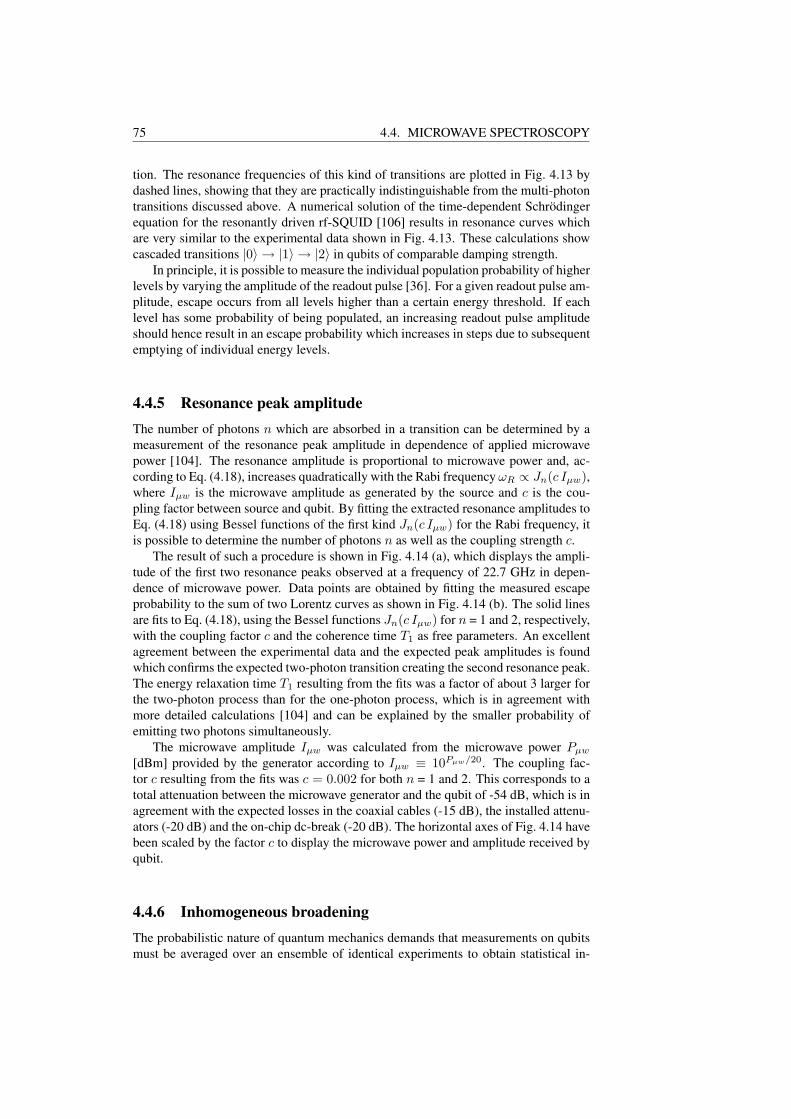
75 4.4. MICROWAVE SPECTROSCOPY
tion. The resonance frequencies of this kind of transitions are plotted in Fig. 4.13 bydashed lines, showing that they are practically indistinguishable from the multi-photontransitions discussed above. A numerical solution of the time-dependent Schrodingerequation for the resonantly driven rf-SQUID [106] results in resonance curves whichare very similar to the experimental data shown in Fig. 4.13. These calculations showcascaded transitions |0〉 → |1〉 → |2〉 in qubits of comparable damping strength.
In principle, it is possible to measure the individual population probability of higherlevels by varying the amplitude of the readout pulse [36]. For a given readout pulse am-plitude, escape occurs from all levels higher than a certain energy threshold. If eachlevel has some probability of being populated, an increasing readout pulse amplitudeshould hence result in an escape probability which increases in steps due to subsequentemptying of individual energy levels.
4.4.5 Resonance peak amplitudeThe number of photons n which are absorbed in a transition can be determined by ameasurement of the resonance peak amplitude in dependence of applied microwavepower [104]. The resonance amplitude is proportional to microwave power and, ac-cording to Eq. (4.18), increases quadratically with the Rabi frequency ωR ∝ Jn(c Iµw),where Iµw is the microwave amplitude as generated by the source and c is the cou-pling factor between source and qubit. By fitting the extracted resonance amplitudes toEq. (4.18) using Bessel functions of the first kind Jn(c Iµw) for the Rabi frequency, itis possible to determine the number of photons n as well as the coupling strength c.
The result of such a procedure is shown in Fig. 4.14 (a), which displays the ampli-tude of the first two resonance peaks observed at a frequency of 22.7 GHz in depen-dence of microwave power. Data points are obtained by fitting the measured escapeprobability to the sum of two Lorentz curves as shown in Fig. 4.14 (b). The solid linesare fits to Eq. (4.18), using the Bessel functions Jn(c Iµw) for n = 1 and 2, respectively,with the coupling factor c and the coherence time T1 as free parameters. An excellentagreement between the experimental data and the expected peak amplitudes is foundwhich confirms the expected two-photon transition creating the second resonance peak.The energy relaxation time T1 resulting from the fits was a factor of about 3 larger forthe two-photon process than for the one-photon process, which is in agreement withmore detailed calculations [104] and can be explained by the smaller probability ofemitting two photons simultaneously.
The microwave amplitude Iµw was calculated from the microwave power Pµw
[dBm] provided by the generator according to Iµw ≡ 10Pµw/20. The coupling fac-tor c resulting from the fits was c = 0.002 for both n = 1 and 2. This corresponds to atotal attenuation between the microwave generator and the qubit of -54 dB, which is inagreement with the expected losses in the coaxial cables (-15 dB), the installed attenu-ators (-20 dB) and the on-chip dc-break (-20 dB). The horizontal axes of Fig. 4.14 havebeen scaled by the factor c to display the microwave power and amplitude received byqubit.
4.4.6 Inhomogeneous broadeningThe probabilistic nature of quantum mechanics demands that measurements on qubitsmust be averaged over an ensemble of identical experiments to obtain statistical in-
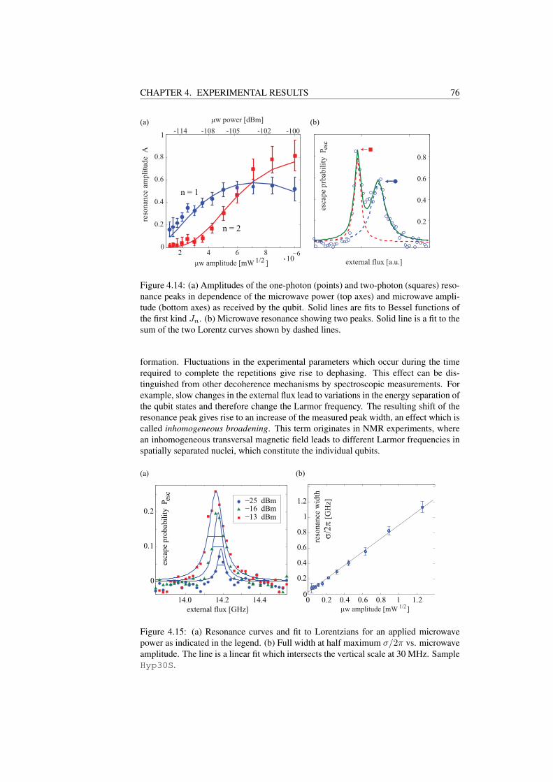
CHAPTER 4. EXPERIMENTAL RESULTS 76
2 4 6 810
−60
0.2
0.4
0.6
0.8
1
µw amplitude [mW ]
reso
nan
ce a
mp
litu
de
A
1/2
-108-114 -100-102
µw power [dBm]
-105
n = 1
n = 20.2
0.4
0.6
0.8
esca
pe
prb
abil
ity
P e
sc
(a) (b)
external flux [a.u.]
Figure 4.14: (a) Amplitudes of the one-photon (points) and two-photon (squares) reso-nance peaks in dependence of the microwave power (top axes) and microwave ampli-tude (bottom axes) as received by the qubit. Solid lines are fits to Bessel functions ofthe first kind Jn. (b) Microwave resonance showing two peaks. Solid line is a fit to thesum of the two Lorentz curves shown by dashed lines.
formation. Fluctuations in the experimental parameters which occur during the timerequired to complete the repetitions give rise to dephasing. This effect can be dis-tinguished from other decoherence mechanisms by spectroscopic measurements. Forexample, slow changes in the external flux lead to variations in the energy separation ofthe qubit states and therefore change the Larmor frequency. The resulting shift of theresonance peak gives rise to an increase of the measured peak width, an effect which iscalled inhomogeneous broadening. This term originates in NMR experiments, wherean inhomogeneous transversal magnetic field leads to different Larmor frequencies inspatially separated nuclei, which constitute the individual qubits.
0 0.2 0.4 0.6 0.8 1 1.20
0.2
0.4
0.6
0.8
1
1.2
µw amplitude [mW ]1/214.2 14.414.0
0
0.1
0.2
external flux [GHz]
−25 dBm−16 dBm−13 dBm
reso
nan
ce w
idth
σ/2
π [
GH
z]
esca
pe
pro
bab
ilit
y
P esc
(a) (b)
Figure 4.15: (a) Resonance curves and fit to Lorentzians for an applied microwavepower as indicated in the legend. (b) Full width at half maximum σ/2π vs. microwaveamplitude. The line is a linear fit which intersects the vertical scale at 30 MHz. SampleHyp30S.
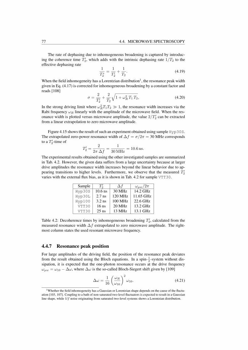
77 4.4. MICROWAVE SPECTROSCOPY
The rate of dephasing due to inhomogeneous broadening is captured by introduc-ing the coherence time T ′2, which adds with the intrinsic dephasing rate 1/T2 to theeffective dephasing rate
1T ∗2
=1T ′2
+1T2
. (4.19)
When the field inhomogeneity has a Lorentzian distribution1, the resonance peak widthgiven in Eq. (4.17) is corrected for inhomogeneous broadening by a constant factor andreads [108]
σ =2T ′2
+2T2
√1 + ω2
R T1 T2, (4.20)
In the strong driving limit where ω2RT1T2 À 1, the resonance width increases via the
Rabi frequency ωR linearly with the amplitude of the microwave field. When the res-onance width is plotted versus microwave amplitude, the value 2/T ′2 can be extractedfrom a linear extrapolation to zero microwave amplitude.
Figure 4.15 shows the result of such an experiment obtained using sample Hyp30S.The extrapolated zero-power resonance width of ∆f = σ/2π = 30 MHz correspondsto a T ′2-time of
T ′2 =2
2π ∆f=
130MHz
= 10.6 ns.
The experimental results obtained using the other investigated samples are summarizedin Tab. 4.2. However, the given data suffers from a large uncertainty because at largerdrive amplitudes the resonance width increases beyond the linear behavior due to ap-pearing transitions to higher levels. Furthermore, we observe that the measured T ′2varies with the external flux bias, as it is shown in Tab. 4.2 for sample VTT30.
Sample T ′2 ∆f ωµw/2πHyp30S 10.6 ns 30 MHz 14.2 GHzHyp30L 2.7 ns 120 MHz 11.65 GHzHyp100 3.2 ns 100 MHz 22.6 GHzVTT30 16 ns 20 MHz 13.2 GHzVTT30 25 ns 13 MHz 13.1 GHz
Table 4.2: Decoherence times by inhomogeneous broadening T ′2, calculated from themeasured resonance width ∆f extrapolated to zero microwave amplitude. The right-most column states the used resonant microwave frequency.
4.4.7 Resonance peak positionFor large amplitudes of the driving field, the position of the resonance peak deviatesfrom the result obtained using the Bloch equations. In a spin- 1
2 -system without dis-sipation, it is expected that the one-photon resonance occurs at the drive frequencyωµw = ω10 −∆ω, where ∆ω is the so-called Bloch-Siegert shift given by [109]
∆ω =116
(ωR
ω10
)2
ω10. (4.21)
1Whether the field inhomogeneity has a Gaussian or Lorentzian shape depends on the cause of the fluctu-ation [103, 107]. Coupling to a bath of non-saturated two-level fluctuators is expected to result in a Gaussianline shape, while 1/f noise originating from saturated two-level systems shows a Lorentzian distribution.

CHAPTER 4. EXPERIMENTAL RESULTS 78
For not too strong driving ωR < ω10, i.e. ωR ∝ Iµw, this equation predicts a smallcorrection to the peak position which scales quadratically in the drive amplitude Iµw.In practical experiments where typically ωR/ω10 < 0.1 and ω10/2π ≈ 10 GHz, theBloch-Siegert shift is about 6 MHz and thus is expected to be negligible.
0 0.2 0.4 0.6 0.8
22.2
22.4
22.6
22.8
µw amplitude [mW ]1/2
reso
nan
ce p
osi
tio
n [
GH
z]
0
200
400
600
[MH
z]0 1.20.4 0.8
µw amplitude [mW ]1/2
ω / 2πR12
∆ω / 2π
(a) (b)
Figure 4.16: (a) Position of resonance, normalized to the applied microwave frequencywhich was 22.8 GHz. (b) Drive amplitude dependence of resonance shift ∆ω (cir-cles) and half the Rabi frequency ωR (squares), both observed at the same microwavefrequency. The two lines have equal slope. Sample Hyp100.
Experimentally, we observe a much stronger influence of the drive amplitude onthe peak position as it is shown in Fig. 4.16 (a). The resonance peak is shifted linearlywith the drive amplitude towards lower frequencies. This is expected for dissipativesystems [103], for which the shift of the resonance frequency can be estimated as
∆ω =ωR
2. (4.22)
This equation is verified by Fig. 4.16 (b), showing the microwave amplitude depen-dence of both the resonance shift ∆ω and half the Rabi frequency ωR/2. The Rabifrequency was obtained by fitting a damped sinusoidal to the coherent oscillations ob-served in the time domain as described in Sec. 4.6. Both kind of data points wereobtained at a microwave frequency of 22.8 GHz in the same measurement run. Theresonance shift shows the same dependence on drive amplitude as half the Rabi fre-quency, and moreover differs absolutely by only a small amount (about 70 MHz for theshown data), hereby clearly confirming Eq. (4.22).
4.4.8 ConclusionsExtensive measurements were done using microwave spectroscopy. In the strong driv-ing regime, we observed transitions to higher levels in the qubit potential well, whichare characterized by additional resonance peaks. A detailed analysis of the resonancepeak amplitudes allowed us to identify the transition mechanism underlying a certainpeak as a two-photon process. We observed a shift of the resonance peak position inthe strong driving limit toward lower frequencies. The magnitude of this shift, which
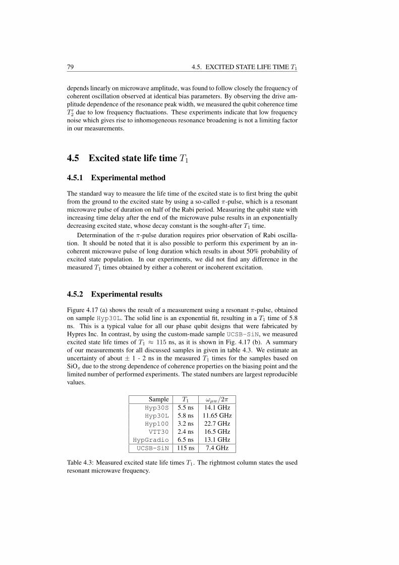
79 4.5. EXCITED STATE LIFE TIME T1
depends linearly on microwave amplitude, was found to follow closely the frequency ofcoherent oscillation observed at identical bias parameters. By observing the drive am-plitude dependence of the resonance peak width, we measured the qubit coherence timeT ′2 due to low frequency fluctuations. These experiments indicate that low frequencynoise which gives rise to inhomogeneous resonance broadening is not a limiting factorin our measurements.
4.5 Excited state life time T1
4.5.1 Experimental method
The standard way to measure the life time of the excited state is to first bring the qubitfrom the ground to the excited state by using a so-called π-pulse, which is a resonantmicrowave pulse of duration on half of the Rabi period. Measuring the qubit state withincreasing time delay after the end of the microwave pulse results in an exponentiallydecreasing excited state, whose decay constant is the sought-after T1 time.
Determination of the π-pulse duration requires prior observation of Rabi oscilla-tion. It should be noted that it is also possible to perform this experiment by an in-coherent microwave pulse of long duration which results in about 50% probability ofexcited state population. In our experiments, we did not find any difference in themeasured T1 times obtained by either a coherent or incoherent excitation.
4.5.2 Experimental results
Figure 4.17 (a) shows the result of a measurement using a resonant π-pulse, obtainedon sample Hyp30L. The solid line is an exponential fit, resulting in a T1 time of 5.8ns. This is a typical value for all our phase qubit designs that were fabricated byHypres Inc. In contrast, by using the custom-made sample UCSB-SiN, we measuredexcited state life times of T1 ≈ 115 ns, as it is shown in Fig. 4.17 (b). A summaryof our measurements for all discussed samples in given in table 4.3. We estimate anuncertainty of about ± 1 - 2 ns in the measured T1 times for the samples based onSiOx due to the strong dependence of coherence properties on the biasing point and thelimited number of performed experiments. The stated numbers are largest reproduciblevalues.
Sample T1 ωµw/2πHyp30S 5.5 ns 14.1 GHzHyp30L 5.8 ns 11.65 GHzHyp100 3.2 ns 22.7 GHzVTT30 2.4 ns 16.5 GHz
HypGradio 6.5 ns 13.1 GHzUCSB-SiN 115 ns 7.4 GHz
Table 4.3: Measured excited state life times T1. The rightmost column states the usedresonant microwave frequency.

CHAPTER 4. EXPERIMENTAL RESULTS 80
0 100 200 300 4000
0.2
0.4
0.6
0.8
readout pulse delay [ns]
esca
pe
pro
bab
ilty
P
esc
readout pulse
µw-π−pulse
0.1
0.2
0.3
0.4
0.5
0.6
0 5 10 15 20 25 30
readout pulse delay [ns]
esca
pe
pro
bab
ilty
P
esc
T 6 ns1~~
T 115 ns1~~
(a)
(b)
0.7
Figure 4.17: Escape probability vs. the delay between populating microwave pulse andreadout pulse as indicated in the inset. Solid lines are fits to an exponential function.(a) Sample Hyp30L, 2000 counts per data point. (b) Sample UCSB-SiN, 1000 countsper data point.
4.5.3 Conclusions
The qubit coherence time T1 due to energy relaxation was measured by directly ob-serving the exponentially decaying population of the excited state in the time domain.The samples fabricated in standard technology using SiO2 as a dielectric for insula-tion between metallic layers showed rather short T1 times of below 8 ns. In a samplewhich was fabricated in a custom process featuring a smaller qubit junction and SiNx
as dielectric, we measured T1 times of about 100 ns. This confirms that the fidelity ofconventionally fabricated phase qubits is limited by a large density of two-level fluctu-ators, which reside in oxide dielectrics and couple to the qubit.

81 4.6. RABI OSCILLATION
4.6 Rabi oscillationApplication of a transverse resonant field induces Rabi oscillations between the twoqubit states as long as the system remains coherent. These oscillations are essential toquantum computation because by this mechanism single qubit operations are realized.The first experimental observations of Rabi oscillation in superconducting qubits weretherefore important milestones in the study of macroscopic quantum coherence andopened the door to the implementation of a solid-state quantum computer.
4.6.1 TheorySolving the Bloch equations (4.12) for the expectation value of the spin’s z-component〈~σz〉 when driven by the rotating transversal field ~Bt(t) results in [108, 103]
〈~σz〉 = e−t/τ1
(sin(ωR t)
ωR τ2+ cos(ωR t)
). (4.23)
This describes an oscillation which is damped with a time constant τ1 given by themean of the coherence times T1 and T2,
2τ1
=1T1
+1T2
. (4.24)
The life time of Rabi oscillation is therefore expected to be a combination of the co-herence times T1 and T2. The oscillation frequency ωR, corrected for damping, reads
ωR =√
γ2B2t − 1/(τ2
2 ), (4.25)
where2τ2
=1T2− 1
T1. (4.26)
For the phase qubit, the transversal driving field is realized by adding a microwavecomponent Iµw sin(ωµwt + ϕ) to the current flowing through the junction. In terms ofthe microwave amplitude Iµw and neglecting damping, the Rabi frequency translatesinto [110]
ωR = γBt =Iµw
2
√1
2~ω10C, (4.27)
where C is the junction capacitance and ω10 the qubit’s Larmor frequency. An actualimplementation of a phase qubit is expected to differ in many aspects from a spin asdescribed by the Bloch equations. Superseding the limitation to non-rotating drivingfields is the existence of higher excited states, which at stronger driving can take partin coherent oscillations. On the other hand, nonlinear and eventually even coherentcoupling to parts of the environment can lead to distinctive features in qubit state evo-lution.
Excitation to higher energy levels
The phase qubit must be operated in a potential well which is made deep enough toavoid escape of the excited state by tunneling. This has the consequence that the po-tential well always contains more than one excited state. Population of the secondexcited state by a microwave which is tuned in resonance to the |0〉 → |1〉 transition

CHAPTER 4. EXPERIMENTAL RESULTS 82
frequency ω10 is expected [111, 112] when the Rabi frequency ωR is comparable tothe anharmonicity ∆ω = ω10 − ω21. As it was shown in Fig. 3.5, the anharmonic-ity of the potential well for typical phase qubits depends on the flux bias and is a fewhundred MHz. Short coherence times in turn dictate observation of Rabi oscillationon a time scale of 10 ns which requires Rabi frequencies of order 100 MHz. For low-quality phase qubits, this leaves only a small parameter range in which transitions tohigher excited states can be avoided. However, theory [113] has shown that a smalloff-resonant transition probability to higher states can be corrected by suitably shapedpulse sequences for sufficiently long coherence times.
Taking into account the possibility of leakage to the second excited qubit state, thepopulation of state |1〉 up to terms quadratical in ωR reads [112]
p1(t) =[1− 3
2
( ωR
2 ∆ω
)2]2
· sin2
ωR
[1−
( ωR
2∆ω
)2]
t
. (4.28)
This equation shows that the oscillation frequency ΩR scales with the amplitude of themicrowave field as
ΩR ∝ Iµw
(1− κ I2
µw
), (4.29)
describing a quadratic bend-off of the observed frequency ΩR from the linear depen-dence on drive amplitude. Equation (4.28) predicts a reduced amplitude of the first ex-cited state population due to leakage into higher states. However, this leakage does notnecessarily reduce the amplitude of observed oscillations, as higher excited states maytake part in coherent oscillations. Modelling a strongly driven phase qubit operatedin the multi-level limit [36] predicted coherent oscillations of nearly 100% amplitudebetween the ground and mostly the 4th and 5th excited states. Since the state readoutvia a dc-flux pulse is usually calibrated to merely distinguish the ground state fromhigher states, the amplitude reduction predicted by Eq. (4.28) may not observed in ourexperiments.
Coupling to parasitic fluctuators
The observation of anti-crossings in the microwave spectrum [27] has demonstratedthat contemporary phase qubits suffer from coherent coupling to parasitic two-levelfluctuators (TLF) which exist in the dielectrics used in junction fabrication. A TLF hasthe two eigenstates |g〉 and |e〉 and is characterized by its resonance frequency ωTLF
and the coupling strength to the qubit J . In resonance at δ = ωTLF − ω10 = 0,the eigenstates of the coupled system are linear combinations of the states |1g〉 and|0e〉 [34]. This gives rise to an oscillatory redistribution of the energy between qubitand parasitic resonator, where the frequency of this oscillation is given by the couplingstrength J which also determines the size of the anti-crossing given by J/h .In a continuously driven qubit-fluctuator system at δ = 0, the probability to measurethe first excited qubit state is calculated [112] as
p1(t) u12
[1− cos
(J t
2~
)cos
(Btt
~
)], (4.30)
where fluctuator damping is neglected and the typical experimental case |Bt|/J À 1is assumed. This equation describes an oscillation at the Rabi frequency ωR = Bt/~

83 4.6. RABI OSCILLATION
which is modulated by the beating frequency J/2~.It has been shown experimentally [34] that the damping rate γ of a TLF can be compa-rable to the qubit decoherence rates. If, in contrast, the parasitic resonators are highlydamped and γ À J , the excited state population will show damped oscillations at asingle frequency,
p1(t) u12
[1− e−J2t/4~γ cos
(Btt
~
)]. (4.31)
4.6.2 Measurement of Rabi oscillation
To observe Rabi oscillation at a chosen microwave frequency, the value of externalflux bias at which the qubit resonance peak is located is first determined by microwavespectroscopy. The duration τµw of the resonant microwave pulse is then varied, herebyadjusting the delay of the calibrated readout pulse such that it always occurs at the endof the microwave pulse. The probability to measure the qubit in the excited state thendisplays the damped oscillations p1(t) described by Eq. (4.28), where the time scale tis given by the microwave pulse duration.
To assure that the readout pulse occurs at the end of the microwave pulse, it maybe necessary to compensate a difference in the signal propagation delay between thecoaxial cables used to send microwave and readout pulses. This is done by sending ananosecond-long resonant microwave pulse of large amplitude and recording the es-cape probability in dependence of the readout pulse delay relative to the microwavepulse. A rapid increase in Pesc then indicates the readout delay at which both pulsesarrive at the qubit simultaneously.
4.6.3 Results of SiOx - based samples
In our experiments on commercially fabricated phase qubits made of niobium as thesuperconductor and SiOx as dielectric, we measured the longest coherence times withsamples of low current density and small qubit junctions. Figure 4.18 shows the bestRabi oscillations which we obtained from such kind of chip using sample Hyp30Sat a driving frequency of ωµw/2π = 13.3 GHz2. Changing the microwave power, weobserve the expected increase of the oscillation frequency.
To extract the oscillation frequency ωR, full amplitude AR and decay time Td, wefit the data to the function
Pesc = P0 + (AR/2) e−t/Td [sin(ωR t + ϕR) + Ab] , (4.32)
as it is shown by the solid line in Fig. 4.18. Here, P0 is a constant offset, ϕR an oscil-lation phase, and Ab is an offset which depends on the current oscillation amplitude.This last fitting parameter is required because at large microwave power we observethat Pesc tends to saturate exponentially after a mean time which is about Td at a highvalue, as it can be seen in the top panel of Fig. 4.18. We may explain this behavior byincoherent population of higher excited states.
2The indicated microwave power or amplitude always corresponds to the signal level at the generatoroutput. If not mentioned explicitly, data has been taken at a temperature of about 20 mK.
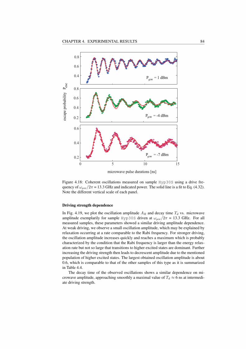
CHAPTER 4. EXPERIMENTAL RESULTS 84
µw
µw
µw
0 5 10 15
0.2
0.4
0.6
0.2
0.4
0.6
0.8
0.4
0.6
0.8
esc
microwave pulse durations [ns]
esca
pe
pro
bab
ilit
y P
P = 1 dBm
P = -4 dBm
P = -7 dBm
Figure 4.18: Coherent oscillations measured on sample Hyp30S using a drive fre-quency of ωµw/2π = 13.3 GHz and indicated power. The solid line is a fit to Eq. (4.32).Note the different vertical scale of each panel.
Driving strength dependence
In Fig. 4.19, we plot the oscillation amplitude AR and decay time Td vs. microwaveamplitude exemplarily for sample Hyp30S driven at ωµw/2π = 13.3 GHz. For allmeasured samples, these parameters showed a similar driving amplitude dependence.At weak driving, we observe a small oscillation amplitude, which may be explained byrelaxation occurring at a rate comparable to the Rabi frequency. For stronger driving,the oscillation amplitude increases quickly and reaches a maximum which is probablycharacterized by the condition that the Rabi frequency is larger than the energy relax-ation rate but not so large that transitions to higher excited states are dominant. Furtherincreasing the driving strength then leads to decrescent amplitude due to the mentionedpopulation of higher excited states. The largest obtained oscillation amplitude is about0.6, which is comparable to that of the other samples of this type as it is summarizedin Table 4.4.
The decay time of the observed oscillations shows a similar dependence on mi-crowave amplitude, approaching smoothly a maximal value of Td ≈ 6 ns at intermedi-ate driving strength.

85 4.6. RABI OSCILLATION
0
0.1
0.3
0.5
0.7
0 0.2 0.4 0.6 0.8 1.00
2
4
6
8
osc
illa
tion d
ecay
tim
e T
[
ns]
d
microwave amplitude [ mW]
osc
illa
tion a
mpli
tud
e A
(a)
(b)
R
Figure 4.19: Dependence of the coherent oscillation amplitude (top panel) and decaytime (bottom panel) on microwave amplitude, measured on sample Hyp30S using adrive frequency of ωµw/2π = 13.3 GHz. Error bars indicate the confidence intervalresulting from the fitting procedure as described in the text. Dashed lines are guides tothe eye.
Sample Td AR ωµw/2π ωR/2πHyp30S 6.0 ns 0.6 12.7 - 14.2 GHz 50 - 900 MHzHyp30L 2.8 ns 0.5 11.65 400 - 1300 MHzHyp100 2.5 ns 0.65 22.6 180 - 550 MHzVTT30 4.0 ns 0.65 12.8 - 17.3 200 - 1800 MHz
Table 4.4: Results of coherent oscillation measurements in SiOx - based samples. Os-cillation decay time Td and amplitude AR are largest obtainable values, averaged overmeasurements using resonant microwaves in the indicated frequency range ωµw andoscillation frequencies ωR. The stated oscillation amplitude AR is not scaled by themeasurement contrast.
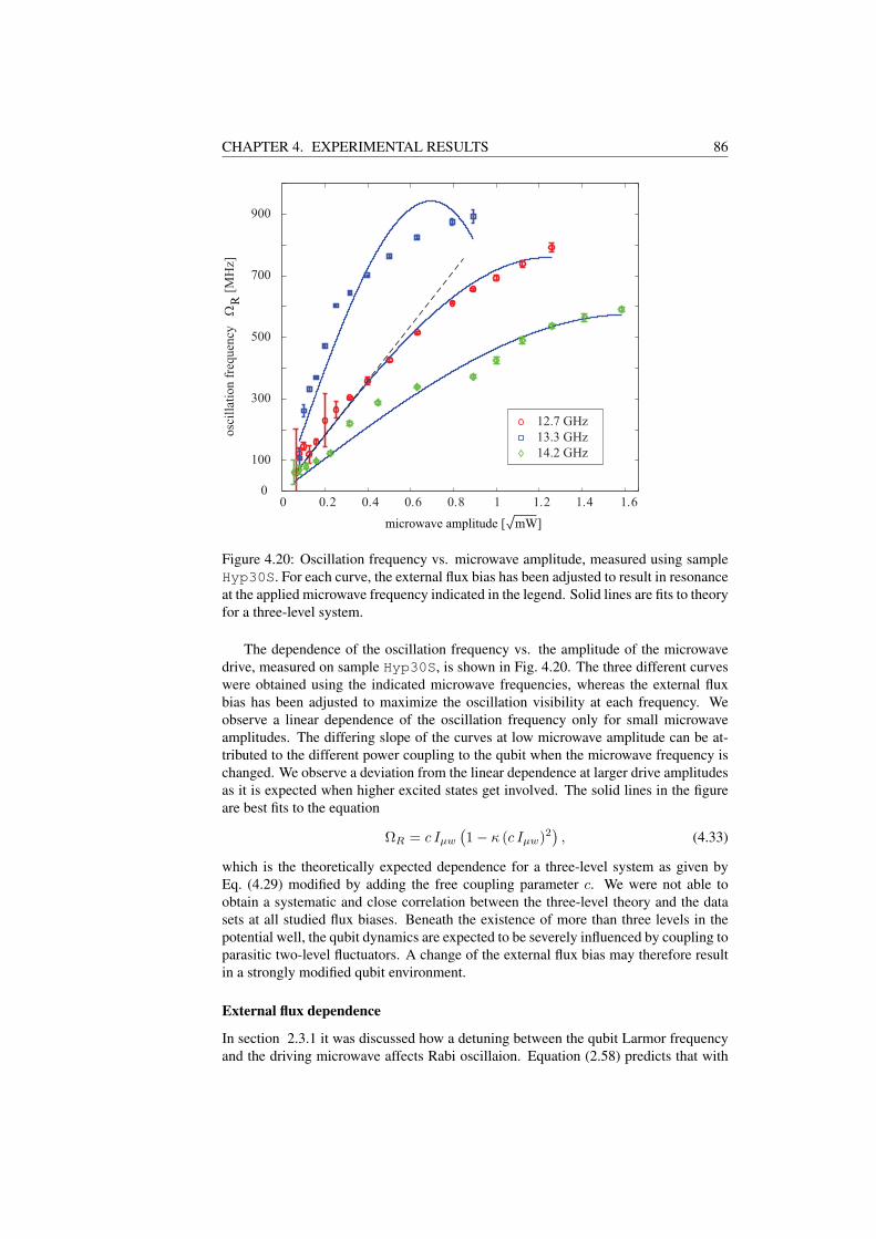
CHAPTER 4. EXPERIMENTAL RESULTS 86
0 0.2 0.4 0.6 0.8 1 1.2 1.4 1.60
100
300
500
700
900
osc
illa
tion f
requen
cy Ω
[MH
z]
12.7 GHz
13.3 GHz
14.2 GHz
microwave amplitude [ mW]
R
Figure 4.20: Oscillation frequency vs. microwave amplitude, measured using sampleHyp30S. For each curve, the external flux bias has been adjusted to result in resonanceat the applied microwave frequency indicated in the legend. Solid lines are fits to theoryfor a three-level system.
The dependence of the oscillation frequency vs. the amplitude of the microwavedrive, measured on sample Hyp30S, is shown in Fig. 4.20. The three different curveswere obtained using the indicated microwave frequencies, whereas the external fluxbias has been adjusted to maximize the oscillation visibility at each frequency. Weobserve a linear dependence of the oscillation frequency only for small microwaveamplitudes. The differing slope of the curves at low microwave amplitude can be at-tributed to the different power coupling to the qubit when the microwave frequency ischanged. We observe a deviation from the linear dependence at larger drive amplitudesas it is expected when higher excited states get involved. The solid lines in the figureare best fits to the equation
ΩR = c Iµw
(1− κ (c Iµw)2
), (4.33)
which is the theoretically expected dependence for a three-level system as given byEq. (4.29) modified by adding the free coupling parameter c. We were not able toobtain a systematic and close correlation between the three-level theory and the datasets at all studied flux biases. Beneath the existence of more than three levels in thepotential well, the qubit dynamics are expected to be severely influenced by coupling toparasitic two-level fluctuators. A change of the external flux bias may therefore resultin a strongly modified qubit environment.
External flux dependence
In section 2.3.1 it was discussed how a detuning between the qubit Larmor frequencyand the driving microwave affects Rabi oscillaion. Equation (2.58) predicts that with

87 4.6. RABI OSCILLATION
increasing detuning ∆ = |ω10 − ωµw| the oscillation frequency is increased, ΩR =√ωR
2 + ∆2, while its amplitude is reduced by a factor ωR2/(ωR
2∆2). Plotting the es-cape probability color coded vs. microwave pulse duration and detuning should there-fore result in the so-called chevron-pattern.
In our current experimental setup, due to the frequency-dependent coupling to thequbit caused by transmission line resonances, it is more convenient to create a detuningby changing the external flux bias rather than the microwave frequency .
800
600
400
200
0
-200
-400
-600
det
un
ing
∆
[M
Hz]
0.7
0.6
0.5
0.4
0.3
0.25 10 15 20 25
microwave pulse duration [ns]
Pesc
Figure 4.21: Escape probability Pesc (color-coded) in dependence of microwave pulseduration and detuning ∆. The detuning was realized by changing the external flux biasat a fixed microwave frequency of 14.2 GHz. Sample Hyp30S.
In Fig. 4.21, a chevron pattern measured using sample Hyp30S driven at ωµw/2π =14.2 GHz is presented. The vertical axis shows the detuning ∆ = (ωµw − ω10)/2π,which was converted from the applied external flux to frequency using spectroscopydata. A linear approximation of the resonance frequency dependence on external fluxin vicinity of the resonance at 14.2 GHz was hereby used.
The figure shows the expected increase of the oscillation frequency when the exter-nal flux is increased starting from the exact resonance, which results in a flatter poten-tial well having a smaller transition frequency ω10 < ωµw. However, close to the exactresonance the oscillation visibility rapidly decreases. We speculate that this is due toan increased probability of inducing transitions to higher levels when the microwavefrequency is slightly smaller than the |0〉 → |1〉 transition frequency, as in this casethe microwave is closer to the |1〉 → |2〉 resonance. Further reducing the detuning for∆ < -500 MHz, the system remains in the ground state, as the microwave frequency isbelow the |0〉 → |1〉 transition frequency.
For the same data, Fig. (4.22) contains plots of the characteristic oscillation pa-rameters obtained by fitting the datasets at each detuning. The oscillation frequencyplotted in Fig. 4.22 (a) follows closely the theoretical detuning dependence as expected

CHAPTER 4. EXPERIMENTAL RESULTS 88
detuning ∆ [MHz]
−600 −400 −200 0 200 400 600 800 1000
400
600
800
1000
0
0.5
1
0
5
10
15
osc
illa
tion
freq
uen
cy [M
Hz]
osc
illa
tion
ampli
tude
Aosc
illa
tion
dec
ay t
ime
T [n
s]R
d
ΩR
(a)
(b)
(c)
Figure 4.22: External flux dependence of the coherent oscillation in sample Hyp30S.(a) oscillation frequency, (b) oscillation amplitude, (c) oscillation decay time.
from Eq. (2.58), which is plotted by the solid line without free parameters. The smalldeviation can be explained by the only approximated flux to frequency conversion.The oscillation amplitude AR shown in Fig. 4.22 (b), in contrast, shows the mentioneddecrease for ∆ / 0. We find a maximum visibility of Rabi oscillation for positive de-tuning. This does not confirm the expectation for a two-state system, which is plottedby the solid line again using Eq. (2.58). The data of extracted oscillation decay timesTd, plotted in Fig. 4.22 (c), suggest that the longest coherence times are obtained closeto resonance, as expected. However, as the oscillation visibility at this point is verysmall, the uncertainty in this data is pretty large.
4.6.4 Results of SiNx - based samplesTo verify that the short coherence times we observed on standardly fabricated sam-ples are not limited by our experimental setup, we also measured the custom-made,high-quality phase qubit sample UCSB-SiN provided by the group of J. Martinis [84].Figure 4.23 contains a selection of Rabi oscillation data which we measured on thissample. Using experimental conditions identical to the measurements described above,we obtained decay times of Td ≈ 110 ns, a factor of about 20 times longer than in thesamples based on Nb-SiOx technology. These data agree with the independent findings[84], and thus it is safe to conclude that our measurement apparatus does not introduce

89 4.6. RABI OSCILLATION
additional sources of decoherence which might affect the qubit dynamics on a timescale of less than 100 ns.
0.2
0.3
0.4
0.3
0.5
0.7
esca
pe
pro
bab
ilit
y
Pes
c
0 50 100 150 2000.2
0.4
0.6
0.8
microwave pulse duration [ns]
P = -27 dBmµw
P = -19 dBmµw
P = -13 dBmµw
Figure 4.23: Rabi oscillation observed in sample UCSB-SiN, using a microwave fre-quency of 6.0 GHz at the indicated powers. At this particular flux bias, the oscillationsshowed a beating.
At certain values of external flux bias, we observe a beating in the coherent oscil-lation amplitude as shown in Fig. 4.23. The beating frequency depends on the Rabifrequency. This can be explained by coherent coupling to a parasitic two-level fluctua-tor as discussed in Sec. 4.6.1. While we observe this effect also in SiOx-based samples,their short coherence times and larger expected density of parasitic fluctuators usuallyhinders observation of more than one beating period.
The dependence of the Rabi oscillation frequency on microwave amplitude is shownin Fig. 4.24 for a set of applied drive frequencies in the range of 6.0 to 8.7 GHz. Simi-larly to SiOx-based samples, the oscillation frequency bends off from the linear depen-dence at large Rabi frequencies. It can be seen from this data that in a shallow potentialwell, corresponding to smaller drive frequencies, bending-off occurs at higher Rabifrequencies than that for the deep potential well. Also, at high drive amplitudes theoscillation frequency appears to saturate at a value which corresponds approximatelyto the anharmonicity of the potential well. For example, at a flux bias resulting in a res-onance frequency of ω10/2π = 6.5 GHz, the anharmonicity is (ω10 − ω21)/2π ≈ 600MHz and at ω10/2π = 8.7 GHz it is ≈ 200 MHz (see Fig. 3.5). However, the curvesobtained at 7.8 GHz and 8.15 GHz driving frequencies fall out of this direct propor-
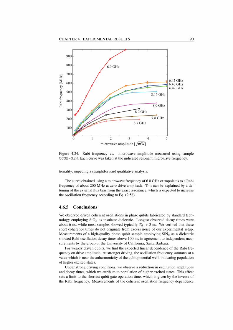
CHAPTER 4. EXPERIMENTAL RESULTS 90
0 1 2 3 4 5
100
200
300
400
500
600
700
800
900
Rab
i fr
equen
cy [
MH
z]
6.0 GHz
6.45 GHz6.40 GHz6.42 GHz
8.15 GHz
8.0 GHz
8.2 GHz
7.8 GHz
8.7 GHz
microwave amplitude [ mW]
Figure 4.24: Rabi frequency vs. microwave amplitude measured using sampleUCSB-SiN. Each curve was taken at the indicated resonant microwave frequency.
tionality, impeding a straightforward qualitative analysis.
The curve obtained using a microwave frequency of 6.0 GHz extrapolates to a Rabifrequency of about 200 MHz at zero drive amplitude. This can be explained by a de-tuning of the external flux bias from the exact resonance, which is expected to increasethe oscillation frequency according to Eq. (2.58).
4.6.5 Conclusions
We observed driven coherent oscillations in phase qubits fabricated by standard tech-nology employing SiOx as insulator dielectric. Longest observed decay times wereabout 6 ns, while most samples showed typically Td ≈ 3 ns. We verified that theseshort coherence times do not originate from excess noise of our experimental setup.Measurements of a high-quality phase qubit sample employing SiNx as a dielectricshowed Rabi oscillation decay times above 100 ns, in agreement to independent mea-surements by the group of the University of California, Santa Barbara.
For weakly driven qubits, we find the expected linear dependence of the Rabi fre-quency on drive amplitude. At stronger driving, the oscillation frequency saturates at avalue which is near the anharmonicity of the qubit potential well, indicating populationof higher excited states.
Under strong driving conditions, we observe a reduction in oscillation amplitudesand decay times, which we attribute to population of higher excited states. This effectsets a limit to the shortest qubit gate operation time, which is given by the inverse ofthe Rabi frequency. Measurements of the coherent oscillation frequency dependence

91 4.7. RAMSEY FRINGES
on drive amplitude support the notion that higher excited states become populated whenthe Rabi frequency is comparable to the qubit anharmonicity.
4.7 Ramsey fringes
4.7.1 TheoryIn the Bloch-sphere representation of the qubit state, Rabi oscillation can be understoodas originating from continuous rotation of the Bloch-vector around the ~x- or the ~y axis.In a Ramsey experiment [114], it is also possible to observe the precession around the~z-axis. Since these rotations do not change the ~z-component of the Bloch vector, theyare not affected by energy relaxation, but only by dephasing. This allows to directlymeasure the effective dephasing rate 1/T ∗2 , which is the sum of the dephasing rate byinhomogeneous broadening and the intrinsic dephasing rate,
1T ∗2
=1T ′2
+1T2
. (4.34)
Iµw 2π
∆t
free precession
0 > z 0 >
1 >
x
y
t
1 >
Φext
t readout
2π
Figure 4.25: Illustration of the Ramsey experiment in the Bloch-sphere representationof the qubit state (top) and sequence of microwave and readout pulses (bottom). (a)A π/2-pulse rotates the Bloch-vector by 90 from |0〉 to the equator. (b) The vectorprecesses freely around the ~z-axis during the time ∆t. (c) A second π/2-pulse projectsthe acquired phase to the ~z-axis. The qubit state is measured by the readout dc-fluxpulse immediately afterwards.
Because only the ~z-component of the Bloch vector is observable, a method is re-quired to realize a phase-dependent projection to the ~z-axis. A pulse sequence suitableto visualize the spin precession and dephasing is illustrated in Fig. 4.25. First, a so-called π/2-pulse is applied, which rotates the Bloch-vector by 90 to the equatorialplane. The duration of such a microwave pulse corresponds to one quarter of the Rabi

CHAPTER 4. EXPERIMENTAL RESULTS 92
oscillation period, as it is determined beforehand at identical bias parameters. Thequbit now undergoes free precession around the ~z-axis at the Larmor frequency ω10.After a variable delay time ∆t, a second π/2-pulse is applied. The outcome of thissecond rotation now depends on the phase acquired during the time interval ∆t.
If the microwave is tuned exactly to the Larmor frequency, it creates an effectivelyconstant transversal field pointing to a fixed direction in the ~x− ~y-plane in the rotatingframe, where no precession occurs. In contrast, if the microwave is detuned from theLarmor frequency, the effective field appears from the rotating frame to be rotatingaround the ~z-axis at the frequency ∆ = ωµw − ω10. In this case, the second π/2-pulsein the Ramsey sequence can be understood as creating a rotation around either the ~x-or ~y-axis, depending on the phase (ωµw − ω10)∆t the microwave pulse acquired withrespect to the rotating frame during the time ∆t. The probability that the second π/2microwave pulse rotates the Bloch vector to the excited state |1〉 therefore oscillates atthe Ramsey frequency
ωRamsey = (ωµw − ω10) = ∆, (4.35)
which is equal to the detuning. Dephasing occurring during the free precession cyclethen gives rise to a Ramsey fringe visibility which decays exponentially at the rate1/T ∗2 .
4.7.2 Experimental resultsFigure 4.26 shows the result of a Ramsey experiment performed on sample UCSB-SiNusing two microwave pulses of frequency 7.7 GHz and duration 1.5 ns, which weredetuned from the Larmor frequency by ≈ 300 MHz.
0 20 40 60 80 100 120
0. 2
0. 4
0. 6
0. 8
free precession time [ns]∆ t
T 90 ns2~~
esca
pe
pro
bab
ilit
y P
esc
*
Figure 4.26: Result of an experiment to measure Ramsey oscillation using sampleUCSB-SiN. The solid line connects measured data points, the dotted line is a fit to asine function decaying exponentially with a time constant of T ∗2 = 90 ns.
The escape probability was measured by applying the readout dc-pulse immediatelyafter the second microwave pulse. It shows the expected oscillation at the detuning

93 4.7. RAMSEY FRINGES
frequency when the separation between the two pulses ∆t is varied. Fitting theseRamsey fringes to an exponentially decaying cosine, as shown by the dotted line inFig. 4.26, results in a dephasing time of T ∗2 ≈ 90 ns, in accordance to independentmeasurements using a similar sample [84].
8.3
8.2
8.1
8.0
7.9
7.8
7.7
7.6
0.9
0.8
0.7
0.6
0.5
0.4
0.3
0.2
0.1
- pulse separation ∆t [ns]π
2
Pesc
mic
row
ave
freq
uen
cy [
GH
z]
0 10 20 30 40 50 60
7.6 7.7 7.8 7.9 8 8.1 8.2 8.3
0
100
200
300
400
microwave frequency [GHz]
Ram
sey
fre
qu
ency
[M
Hz]
(a)
(b)
Figure 4.27: (a) Escape probability (color-coded) vs. the time delay between two π/2-pulses and the microwave frequency. Ramsey oscillation is observed at all frequenciesexcept near the exact resonance close to 8.0 GHz. (b) Ramsey oscillation frequency vs.microwave frequency used to generate the π/2-pulses. Dashed lines have unity slopeand originate at 8.0 GHz.
The amplitude of the Ramsey oscillation shows a low-frequency beating. This isexpected to originate from the finite duration of the microwave π/2-pulses, duringwhich some precession occurs when the detuning is large. In an improved pulse se-quence [101], this is circumvented by using two π/2-pulses always at exact resonanceand creating the detuning by a change of the Larmor frequency through a dc-flux pulsebetween the microwave pulses.
To check whether the observed Ramsey frequency indeed corresponds to the de-tuning, we repeated the measurement for several microwave frequencies. This data is
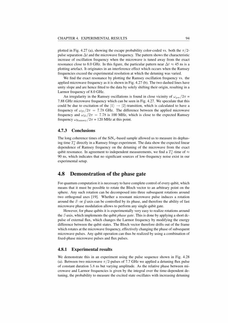
CHAPTER 4. EXPERIMENTAL RESULTS 94
plotted in Fig. 4.27 (a), showing the escape probability color-coded vs. both the π/2-pulse separation ∆t and the microwave frequency. The pattern shows the characteristicincrease of oscillation frequency when the microwave is tuned away from the exactresonance close to 8.0 GHz. In this figure, the particular pattern near ∆t ≈ 45 ns is aplotting artefact. It originates in an interference effect which occurs when the Ramseyfrequencies exceed the experimental resolution at which the detuning was varied.
We find the exact resonance by plotting the Ramsey oscillation frequency vs. theapplied microwave frequency as it is shown in Fig. 4.27 (b). The two dashed lines haveunity slope and are hence fitted to the data by solely shifting their origin, resulting in aLarmor frequency of 8.0 GHz.
An irregularity in the Ramsey oscillations is found in close vicinity of ωµw/2π =7.88 GHz microwave frequency which can be seen in Fig. 4.27. We speculate that thiscould be due to excitation of the |1〉 → |2〉-transition, which is calculated to have afrequency of ω21/2π = 7.78 GHz. The difference between the applied microwavefrequency and ω21/2π = 7.78 is 100 MHz, which is close to the expected Ramseyfrequency ωRamsey/2π = 120 MHz at this point.
4.7.3 ConclusionsThe long coherence times of the SiNx-based sample allowed us to measure its dephas-ing time T ∗2 directly in a Ramsey fringe experiment. The data show the expected lineardependence of Ramsey frequency on the detuning of the microwave from the exactqubit resonance. In agreement to independent measurements, we find a T ∗2 -time of ≈90 ns, which indicates that no significant sources of low-frequency noise exist in ourexperimental setup.
4.8 Demonstration of the phase gateFor quantum computation it is necessary to have complete control of every qubit, whichmeans that it must be possible to rotate the Bloch vector to an arbitrary point on thesphere. Any such rotation can be decomposed into three subsequent rotations aroundtwo orthogonal axes [19]. Whether a resonant microwave pulse induces a rotationaround the ~x- or ~y-axis can be controlled by its phase, and therefore the ability of fastmicrowave phase modulation allows to perform any single qubit gate.
However, for phase qubits it is experimentally very easy to realize rotations aroundthe ~z-axis, which implements the qubit phase gate. This is done by applying a short dc-pulse of external flux, which changes the Larmor frequency by modifying the energydifference between the qubit states. The Bloch vector therefore drifts out of the framewhich rotates at the microwave frequency, effectively changing the phase of subsequentmicrowave pulses. Any qubit operation can thus be realized by using a combination offixed-phase microwave pulses and flux pulses.
4.8.1 Experimental resultsWe demonstrate this in an experiment using the pulse sequence shown in Fig. 4.28(a). Between two microwave π/2-pulses of 7.7 GHz we applied a detuning flux pulseof constant duration 5.8 ns but varying amplitude. As the relative phase between mi-crowave and Larmor frequencies is given by the integral over the time-dependent de-tuning, the probability to measure the excited state oscillates with increasing detuning
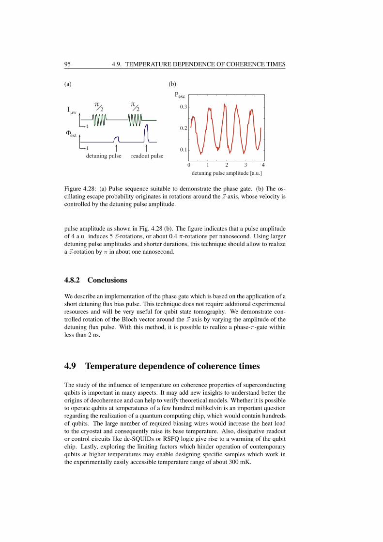
95 4.9. TEMPERATURE DEPENDENCE OF COHERENCE TIMES
4 3 2 10
0.1
0.2
0.3
detuning pulse amplitude [a.u.]
detuning pulse readout pulse
P
2π
2π
esc
(a) (b)
Iµw
tΦ
t
ext
Figure 4.28: (a) Pulse sequence suitable to demonstrate the phase gate. (b) The os-cillating escape probability originates in rotations around the ~z-axis, whose velocity iscontrolled by the detuning pulse amplitude.
pulse amplitude as shown in Fig. 4.28 (b). The figure indicates that a pulse amplitudeof 4 a.u. induces 5 ~z-rotations, or about 0.4 π-rotations per nanosecond. Using largerdetuning pulse amplitudes and shorter durations, this technique should allow to realizea ~z-rotation by π in about one nanosecond.
4.8.2 Conclusions
We describe an implementation of the phase gate which is based on the application of ashort detuning flux bias pulse. This technique does not require additional experimentalresources and will be very useful for qubit state tomography. We demonstrate con-trolled rotation of the Bloch vector around the ~z-axis by varying the amplitude of thedetuning flux pulse. With this method, it is possible to realize a phase-π-gate withinless than 2 ns.
4.9 Temperature dependence of coherence times
The study of the influence of temperature on coherence properties of superconductingqubits is important in many aspects. It may add new insights to understand better theorigins of decoherence and can help to verify theoretical models. Whether it is possibleto operate qubits at temperatures of a few hundred milikelvin is an important questionregarding the realization of a quantum computing chip, which would contain hundredsof qubits. The large number of required biasing wires would increase the heat loadto the cryostat and consequently raise its base temperature. Also, dissipative readoutor control circuits like dc-SQUIDs or RSFQ logic give rise to a warming of the qubitchip. Lastly, exploring the limiting factors which hinder operation of contemporaryqubits at higher temperatures may enable designing specific samples which work inthe experimentally easily accessible temperature range of about 300 mK.

CHAPTER 4. EXPERIMENTAL RESULTS 96
4.9.1 TheoryWhen it is possible to truncate the phase qubit to a two-level system it can be describedas a spin-1/2 system which has the Hamiltonian
Hq = −12~∆σx +
12εσz, (4.36)
where ε is the difference of state energies and 12~∆ is the transition matrix element. If
the latter is large, the system oscillates between its two states at the Rabi frequency ∆.
Decoherence is modelled in the Caldeira-Leggett approach [52] as resulting fromcoupling of the spin to an infinite set of harmonic oscillators. The dilemma that whilequantum mechanics requires a system to evolve unitarily but dissipation is experiencedas a non-reversible effect is hereby solved - the energy is distributed among a largenumber of degrees of freedom and unlikely to return to the spin. The coupled systemis thus described by the so-called ”spin-boson” Hamiltonian [52, 115, 60]
H = Hq +∑α
(12mαω2
αx2α +
p2α
2mα
)+
12q0σz
∑α
Cαxα, (4.37)
where the second term summarizes the α harmonic oscillators of the bath, each having acoordinate xα , mass mα, momentum pα and eigen frequency ωα. The third term addsthe interaction between the spin and the bath, where a linear coupling of strength Cα
between the coordinates of the oscillators and the z-component of the spin is assumed.In thermal equilibrium, all information about the boson bath is contained in the
spectral density function J(ω) [115]
J(ω) =π
2~∑α
C2α
mα ωαδ(ω − ωα), (4.38)
where the Dirac δ-functions add to a continuous function in the limit of infinitely manybath modes [60]. For an electric circuit having an impedance Z(ω), the spectral densityfunction is [60]
J(ω) = ωRQ
Re[Z(ω)], (4.39)
where RQ = h/(2e)2 is the superconducting resistance quantum and Re[Z(ω)] de-notes the real part of the circuit impedance.
Knowledge of the noise spectrum allows to derive the temperature dependence ofthe relaxation time T1 and dephasing time T2 [115, 116, 117, 118]. For finite temper-ature T ,
T−11 ∝ J(ω) coth
~ω2kBT
ω→∆E/~(4.40)
T−12 ∝ T−1
1
2ω→∆E/~
+ J(ω) coth~ω
2kBTω→0
. (4.41)
Equation (4.40) shows that the relaxation rate is only affected by bath modes at thequbit frequency ω10 = ∆E/~. The dephasing rate Eq. (4.41) has a contribution from
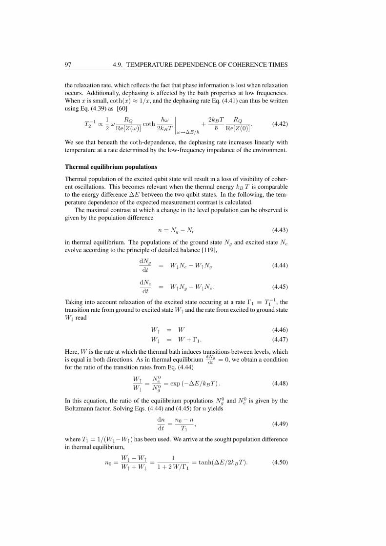
97 4.9. TEMPERATURE DEPENDENCE OF COHERENCE TIMES
the relaxation rate, which reflects the fact that phase information is lost when relaxationoccurs. Additionally, dephasing is affected by the bath properties at low frequencies.When x is small, coth(x) ≈ 1/x, and the dephasing rate Eq. (4.41) can thus be writtenusing Eq. (4.39) as [60]
T−12 ∝ 1
2ω
RQ
Re[Z(ω)]coth
~ω2kBT
ω→∆E/~+
2kBT
~RQ
Re[Z(0)]. (4.42)
We see that beneath the coth-dependence, the dephasing rate increases linearly withtemperature at a rate determined by the low-frequency impedance of the environment.
Thermal equilibrium populations
Thermal population of the excited qubit state will result in a loss of visibility of coher-ent oscillations. This becomes relevant when the thermal energy kB T is comparableto the energy difference ∆E between the two qubit states. In the following, the tem-perature dependence of the expected measurement contrast is calculated.
The maximal contrast at which a change in the level population can be observed isgiven by the population difference
n = Ng −Ne (4.43)
in thermal equilibrium. The populations of the ground state Ng and excited state Ne
evolve according to the principle of detailed balance [119],
dNg
dt= W↓Ne −W↑Ng (4.44)
dNe
dt= W↑Ng −W↓Ne. (4.45)
Taking into account relaxation of the excited state occuring at a rate Γ1 ≡ T−11 , the
transition rate from ground to excited state W↑ and the rate from excited to ground stateW↓ read
W↑ = W (4.46)W↓ = W + Γ1. (4.47)
Here, W is the rate at which the thermal bath induces transitions between levels, whichis equal in both directions. As in thermal equilibrium dNg
dt = 0, we obtain a conditionfor the ratio of the transition rates from Eq. (4.44)
W↑W↓
=N0
e
N0g
= exp (−∆E/kBT ) . (4.48)
In this equation, the ratio of the equilibrium populations N0g and N0
e is given by theBoltzmann factor. Solving Eqs. (4.44) and (4.45) for n yields
dn
dt=
n0 − n
T1, (4.49)
where T1 = 1/(W↓−W↑) has been used. We arrive at the sought population differencein thermal equilibrium,
n0 =W↓ −W↑W↑ + W↓
=1
1 + 2 W/Γ1= tanh(∆E/2kBT ). (4.50)

CHAPTER 4. EXPERIMENTAL RESULTS 98
The last expression, which is the most important result of this section, has been ob-tained using Eq. (4.48) and the identity
tanh(∆E/2kBT ) =1− exp(∆E/kBT )1 + exp(∆E/kBT )
. (4.51)
The maximal measurement contrast, assuming that it is limited only by the thermal bathequilibrating the population of the two qubit levels, hence follows the tanh dependencegiven in Eq. (4.50). At the temperature where kBT = ∆E, the contrast is expected todrop to n0 = 46 %.
Integration of Eq. (4.49) shows that the system reaches thermal equilibrium after amean time which is equal to the energy relaxation time T1:
n(t) = n0
(1− e−t/T1
). (4.52)
A similar calculation is used to find the equilibrium population difference nD in adriven system. In the incoherent limit, the drive gives rise to a transition rate ΓD whichis equal for both directions |g〉 ↔ |e〉, similar as the thermal bath. Detailed balance inthis case results in
dnD
dt= −2ΓD n. (4.53)
Finally, combining the rates Eq. (4.53) and Eq. (4.49),
dnD0
dt= −2Wn +
n0 − n
T1, (4.54)
we arrive at the population difference nD0 in steady state dnD0/dt = 0 for the continu-ously driven system coupled to a thermal bath,
nD0 =n0
1 + 2W/Γ1. (4.55)
4.9.2 Measurement limitationsIn order to observe the phase dynamics at higher temperatures it is essential to avoidthermal activation out of the shallow potential well. As it was discussed in Sec. 2.2.5,the activation rate increases exponentially as the potential barrier height becomes com-parable to the thermal energy kBT . At high temperatures it is therefore required tooperate in a deep potential well where thermal activation can be neglected.
On the other hand, the possibility to use an rf-SQUID as a quantum bit is build onthe ability to truncate it to a two-state system. This requires the qubit potential to besufficiently anharmonic, hereby separating higher states through the different transitionfrequencies between neighboring levels. However, as energy relaxation (and tunneling)give rise to a certain width of each energy level, this is only guaranteed as long as thecondition
~ω21 +12(δE1 + δE2) ¿ ~ω01 (4.56)
is satisfied. Here, δEn is the full width of level n arising from its finite lifetime τn andωfi is the transition frequency from level i to level f , see Fig. 4.29 for illustration. Thefinite width of the ground state is hereby given by the tunnel rate through the potentialbarrier.
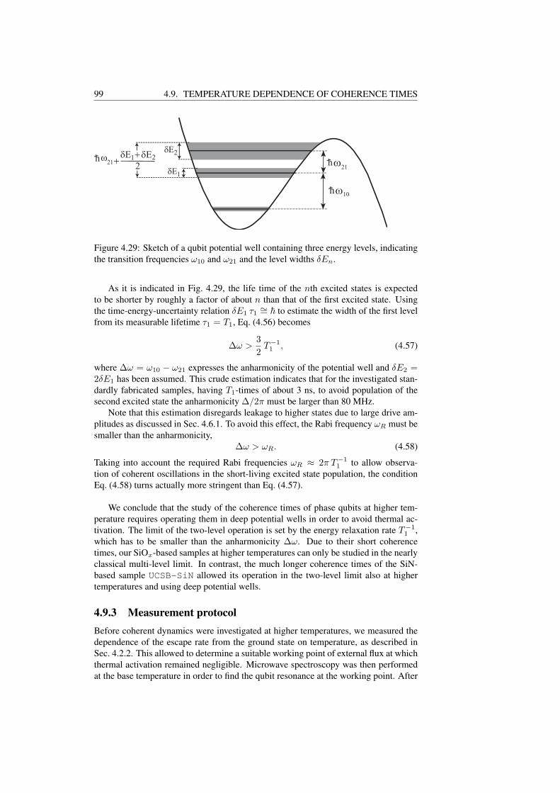
99 4.9. TEMPERATURE DEPENDENCE OF COHERENCE TIMES
δΕ2
ω21
ω10
δE1
h
h ω
21h
δE1 δE2+
2+
Figure 4.29: Sketch of a qubit potential well containing three energy levels, indicatingthe transition frequencies ω10 and ω21 and the level widths δEn.
As it is indicated in Fig. 4.29, the life time of the nth excited states is expectedto be shorter by roughly a factor of about n than that of the first excited state. Usingthe time-energy-uncertainty relation δE1 τ1
∼= ~ to estimate the width of the first levelfrom its measurable lifetime τ1 = T1, Eq. (4.56) becomes
∆ω >32
T−11 , (4.57)
where ∆ω = ω10 − ω21 expresses the anharmonicity of the potential well and δE2 =2δE1 has been assumed. This crude estimation indicates that for the investigated stan-dardly fabricated samples, having T1-times of about 3 ns, to avoid population of thesecond excited state the anharmonicity ∆/2π must be larger than 80 MHz.
Note that this estimation disregards leakage to higher states due to large drive am-plitudes as discussed in Sec. 4.6.1. To avoid this effect, the Rabi frequency ωR must besmaller than the anharmonicity,
∆ω > ωR. (4.58)
Taking into account the required Rabi frequencies ωR ≈ 2π T−11 to allow observa-
tion of coherent oscillations in the short-living excited state population, the conditionEq. (4.58) turns actually more stringent than Eq. (4.57).
We conclude that the study of the coherence times of phase qubits at higher tem-perature requires operating them in deep potential wells in order to avoid thermal ac-tivation. The limit of the two-level operation is set by the energy relaxation rate T−1
1 ,which has to be smaller than the anharmonicity ∆ω. Due to their short coherencetimes, our SiOx-based samples at higher temperatures can only be studied in the nearlyclassical multi-level limit. In contrast, the much longer coherence times of the SiN-based sample UCSB-SiN allowed its operation in the two-level limit also at highertemperatures and using deep potential wells.
4.9.3 Measurement protocolBefore coherent dynamics were investigated at higher temperatures, we measured thedependence of the escape rate from the ground state on temperature, as described inSec. 4.2.2. This allowed to determine a suitable working point of external flux at whichthermal activation remained negligible. Microwave spectroscopy was then performedat the base temperature in order to find the qubit resonance at the working point. After

CHAPTER 4. EXPERIMENTAL RESULTS 100
observation of coherent oscillations at the working point, external flux bias, microwavefrequency and amplitude were varied by small amounts in order to maximize the oscil-lation amplitude and life time.
All measurements presented in the remainder of this chapter were obtained whilekeeping the qubit bias parameters constant at all temperatures. In order to preservehigh measurement contrast the amplitude of the readout pulse had to be reduced athigh temperatures, where qubit escape from the excited state to the deep well becomespossible not only by quantum tunnelling but also by thermal activation over the barrier.We adjusted the readout amplitude at each temperature by the automated calibrationprocedure described in Sec. 4.3.5.
The width of the measured switching-current histogram of the readout dc-SQUIDincreases in the thermal regime, which reduces the contrast between the two qubitstates. We therefore separated the contributions of the two states to the readout SQUIDswitching-current distribution by the fitting procedure using weighted histograms ofthe two flux states as described in Sec. 3.4.2.
A complete data set to observe the temperature dependence of coherent oscillationconsists of approximately 8000 histograms. At each of the typically 40 temperaturevalues in the range of 20 mK to 800 mK, the escape probability was probed for about200 values of the microwave pulse duration. As each histogram comprises at least 1000measurements, in total about 8 million measurements were acquired at a typical rate of300 measurements per second. Up to five minutes were necessary to allow for stabi-lization of the dilution unit temperature at every set point. One complete measurementthus took a time of more than 10 hours. The stability of the external qubit parametersduring this time was guaranteed by using a mains supply to energize the biasing elec-tronics. It was impossible to measure in an automated fashion at temperatures above800 mK because the He3/He4-mixture began to evaporate at about 900 mK.
4.9.4 Temperature dependence of Rabi oscillations
Results of SiOx - based samples
We measured the influence of temperature on coherent oscillations in the SiOx basedsamples Hyp30S and VTT30, both having comparable coherence times and qubit pa-rameters. In the following we only present results obtained on sample VTT30, whichwere similar to those acquired using the other sample.
Figure 4.30 (a) displays coherent oscillations in sample VTT30 at the indicatedtemperatures. The microwave drive frequency was ωµw/2π = 16.5 GHz and its ampli-tude was adjusted to result in a coherent oscillation frequency of ωR/2π = 750 MHz.For the same bias parameters, Fig. 4.30 (a) contains the result of a measurement of theoscillation frequency dependence on drive amplitude, indicating that the chosen ampli-tude of ≈ 0.28
√mW was small enough to remain in the linear regime. The observed
oscillations decay at the lowest temperature with a time constant of about 4 ns, as it istypical for all our SiOx - based samples. Remarkably, even at the highest temperatureof 800 mK oscillations can be clearly seen, though their amplitude and decay time areboth reduced by about a factor of 2.
A systematic evaluation of the temperature dependence of coherent oscillation am-plitude and decay time is given by the data presented in Fig. 4.31, using the fittingprocedure described in Sec. 4.6.3. This figure also includes measurements using dif-

101 4.9. TEMPERATURE DEPENDENCE OF COHERENCE TIMES
0 2 4 6 8 10 12 140
0.5
1
1.5
2
2.5
microwave pulse duration [ns]
T = 20 mK
T = 220 mK
T = 420 mK
T = 620 mK
T = 800 mK
0 0.2 0.4 0.6 0.8
200
600
1000
1400
osc
illa
tio
n f
req
uen
cy [
MH
z]
microwave amplitude [ mW]
esca
pe
pro
bab
ilit
y
Pes
c
(a)
(b)
Figure 4.30: (a) Coherent oscillations observed using sample VTT30, driven at 16.5GHz microwave frequency and amplitude 0.28
√mW, at the indicated temperatures.
Each curve is offset by Pesc=0.5 for clarity. (b) Coherent oscillation frequency vs.microwave drive amplitude at identical bias parameters, measured at T=20 mK.
ferent external flux biases, corresponding to qubit resonances at 15.7 GHz, 16.5 GHzand 17.3 GHz. At 15.7 GHz, the coherent oscillation frequency was ωR/2π = 750MHz and thus equal to the 16.5 GHz data, while for 17.3 GHz it was with ωR/2π =830 MHz about 10 % larger. The oscillation frequency changed with temperature lessthan ≈ 2 %, which is within the confidence intervals of the fits. Figure 4.31 (a) showsthat for all datasets the oscillation amplitude remained unchanged below a temperatureof about 200 mK and then decreased monotonically to approximately 50% of its valueat the highest measured temperature of 800 mK. The solid lines in this figure are plots

CHAPTER 4. EXPERIMENTAL RESULTS 102
0.3
0.4
0.5
0.6
0.7
0.8
osc
illa
tion a
mpli
tude
0 0.2 0.4 0.6 0.8 1
1.5
2
2.5
3
3.5
4
Temperature [K]
osc
illa
tion d
ecay
ti
me
[ns]
17.3 GHz
16.5 GHz
15.7 GHz
17.3 GHz
16.5 GHz
15.7 GHz
4.5
Figure 4.31: (a) Coherent oscillation amplitude (top) and decay time (bottom) ver-sus temperature, measured using sample VTT30. Each data set corresponds to anadjusted magnetic field resulting in resonance at the applied microwave frequencyωµw/2π indicated in the legend. In (a), the solid lines show the expected contrastfollowing C0 · tanh(~ωµw/2kBT ) and the dashed line is the expected contrast for a|0〉 ↔ |2〉-oscillation. In (b), the solid lines show the expected T1-times Eq. (4.60) for∆E = ~ωµw. Error bars in the insets give average confidence intervals of the fits.
to the equation
C(T ) = C0 tanh(~ωµw
2kBT
), (4.59)
which according to Eq. (4.50) is the theoretical expectation for the oscillation visibilityreduction due to thermal population of the first excited qubit state. For these plots, C0
was set to the observed amplitude at the lowest temperature and ωµw corresponds to theapplied microwave frequency. The oscillation amplitude measured in the most shallowpotential well using 15.7 GHz microwave frequency does indeed show the expected

103 4.9. TEMPERATURE DEPENDENCE OF COHERENCE TIMES
temperature dependence, while the other two data sets display a larger amplitude thanexpected at high temperatures. This could be explained by assuming that the oscillationin the deeper potential wells involves the second excited state, which is less affected bythermal population due to its about twice larger energy. The dashed line in Fig. 4.31 (a)is a plot of Eq. (4.51) using ωµw/2π = 2·16.5 GHz to show the expected contrast of a|0〉 ↔ |2〉 oscillation. However, as it was pointed out before, the effective environmentof the qubit may change drastically when changing the flux bias due to coupling toparasitic fluctuators, rendering a quantitative analysis difficult.
The temperature dependence of the oscillation lifetime obtained from the same datais shown in Fig. 4.31 (b). The difference in the absolute values of the lifetimes whenchanging the flux bias may be interpreted either as being due to varying coupling toparasitic resonators or to an increased probability of leakage to higher levels for deeperpotential wells. For phase qubits, the expected temperature dependence of the energyrelaxation time was given by Eq. (3.1.2), which is shown in the figure by the solid linesbeing plots of the equation
T1 = 2 T 01
[1 + coth
(∆E
2kBT
)]−1
, (4.60)
where ∆E = ~ωµw was the applied microwave frequency and T 01 is the fitting pa-
rameter for the lifetime at zero temperature. In contrast to the oscillation amplitude,the theoretical expectation for the relaxation time is more closely met by the datasetsobtained at 16.5 GHz and 17.3 GHz driving frequencies. The dataset obtained at 15.7GHz shows a weaker temperature dependence. As it was mentioned in Sec. 4.6.1, thedecay rate of Rabi oscillation is determined by the mean of relaxation and dephasingrates. Comparing the decay rate of Rabi oscillation to the temperature dependence ofthe T1 time is therefore inaccurate. Nevertheless, relaxation contributes a large part tothe dephasing rate as it was shown by Eq. (4.41).
Results of the SiNx - based sample
The temperature dependence of coherent oscillations in the high-quality qubit sampleUCSB-SiN was measured using microwave frequencies in the range of 7.4 GHz to 8.7GHz. Figure 4.32 exemplarily shows data obtained using 7.4 GHz drive frequency atthree temperatures. At 15 mK, the oscillations showed a life time of about 100 ns andan amplitude corrected for histogram overlap of about 0.85, whereas at 335 mK bothamplitude and life time were substantially smaller. The results obtained by fitting theoscillations to exponentially decaying sine functions are summarized in Fig. 4.33 forthree external flux biases adjusted to result in resonance at the chosen microwave drivefrequency indicated in the legends.
The oscillation amplitudes display a distinct behavior which is shown in Fig. 4.33(a). Increasing the temperature, the amplitude of the oscillation taken at 7.4 GHz is re-duced slowly up to a temperature of about 250 mK, beyond which it decreases rapidlyand reaches zero at 350 mK. The data for 8.0 GHz microwave frequency does notdepend on temperature below about 300 mK, but quickly approaches zero close to400 mK. Most peculiar, the oscillation amplitude recorded using 8.7 GHz drive fre-quency first drops by about 30 % at 200 mK, but with further increasing the temper-ature reaches a maximum value at 315 mK, which is actually larger than its value at15 mK. Beyond the maximum, the oscillation decays quickly and at a similar rate as
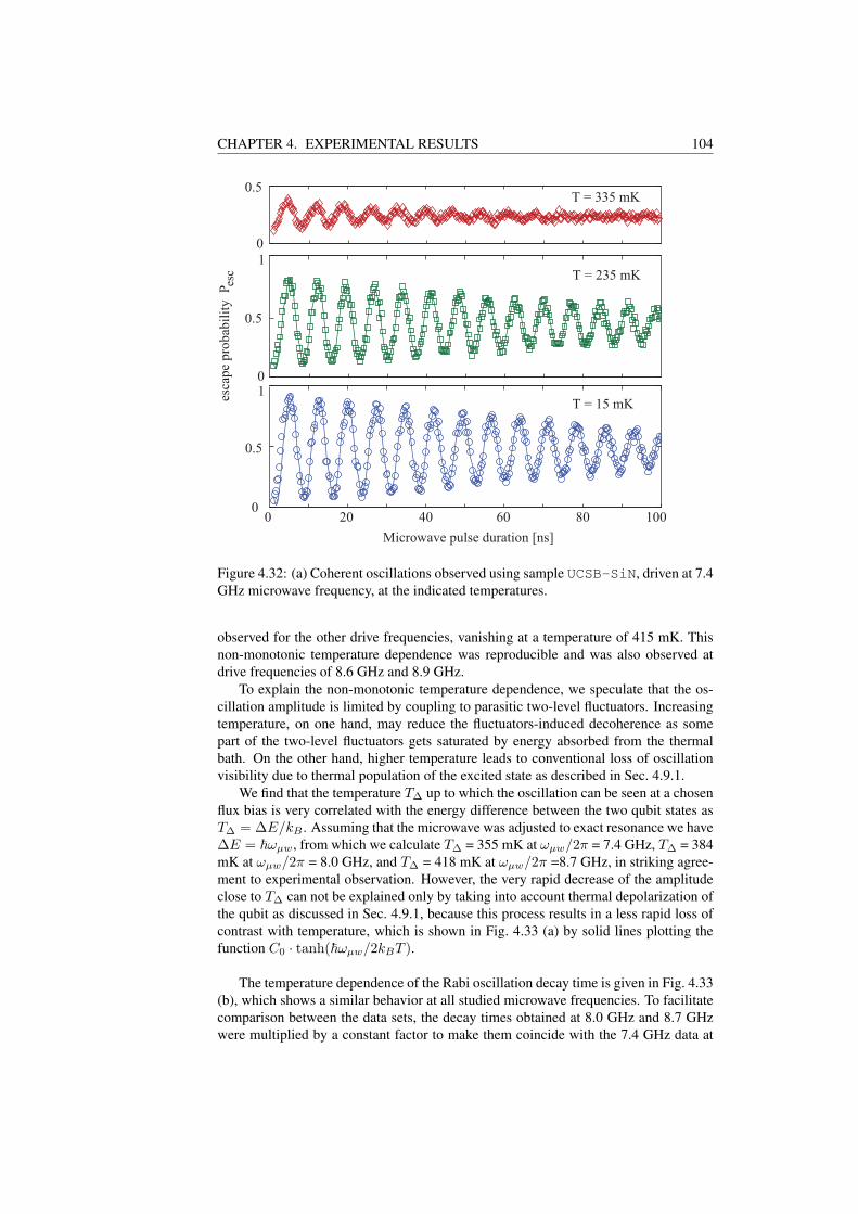
CHAPTER 4. EXPERIMENTAL RESULTS 104
0 20 40 60 80 1000
0.5
1
0.5
0
0.5
Microwave pulse duration [ns]
T = 15 mK
T = 235 mK
T = 335 mK
1
0
esca
pe
pro
bab
ilit
y P
esc
Figure 4.32: (a) Coherent oscillations observed using sample UCSB-SiN, driven at 7.4GHz microwave frequency, at the indicated temperatures.
observed for the other drive frequencies, vanishing at a temperature of 415 mK. Thisnon-monotonic temperature dependence was reproducible and was also observed atdrive frequencies of 8.6 GHz and 8.9 GHz.
To explain the non-monotonic temperature dependence, we speculate that the os-cillation amplitude is limited by coupling to parasitic two-level fluctuators. Increasingtemperature, on one hand, may reduce the fluctuators-induced decoherence as somepart of the two-level fluctuators gets saturated by energy absorbed from the thermalbath. On the other hand, higher temperature leads to conventional loss of oscillationvisibility due to thermal population of the excited state as described in Sec. 4.9.1.
We find that the temperature T∆ up to which the oscillation can be seen at a chosenflux bias is very correlated with the energy difference between the two qubit states asT∆ = ∆E/kB . Assuming that the microwave was adjusted to exact resonance we have∆E = ~ωµw, from which we calculate T∆ = 355 mK at ωµw/2π = 7.4 GHz, T∆ = 384mK at ωµw/2π = 8.0 GHz, and T∆ = 418 mK at ωµw/2π =8.7 GHz, in striking agree-ment to experimental observation. However, the very rapid decrease of the amplitudeclose to T∆ can not be explained only by taking into account thermal depolarization ofthe qubit as discussed in Sec. 4.9.1, because this process results in a less rapid loss ofcontrast with temperature, which is shown in Fig. 4.33 (a) by solid lines plotting thefunction C0 · tanh(~ωµw/2kBT ).
The temperature dependence of the Rabi oscillation decay time is given in Fig. 4.33(b), which shows a similar behavior at all studied microwave frequencies. To facilitatecomparison between the data sets, the decay times obtained at 8.0 GHz and 8.7 GHzwere multiplied by a constant factor to make them coincide with the 7.4 GHz data at

105 4.9. TEMPERATURE DEPENDENCE OF COHERENCE TIMES
0
0.2
0.4
0.6
0.8
1
osc
ilat
ion a
mpli
tude
7.4 GHz
8 GHz
8.7 GHz
0 0.1 0.2 0.3 0.4 0.50
20
40
60
80
100
120
Temperature [K]
osc
illa
tion d
ecay
tim
e [n
s]
7.4 GHz
8 GHz
8.7 GHz
(a)
(b)
Figure 4.33: (a) Amplitude of coherent oscillation vs. temperature obtained at theindicated microwave frequency ωµw/2π. Solid lines: expected contrast followingC0 · tanh(~ωµw/2kBT ), dashed line: expected contrast for a |0〉 ↔ |2〉-oscillation.(b) Coherent oscillation lifetime Td vs. temperature. Solid lines: expected T1-timeEq. (4.60) for ∆E = ~ωµw, dashed line: Eq. (4.60) for ∆E = 2 ~ωµw for ωµw/2π=8.0GHz.
the temperature of 15 mK. These decay times at the lowest temperature were 29.5 ns at8.0 GHz and 42.5 ns at 8.7 GHz. The scaled plots show that the oscillation decay timedoes not depend on temperature up to about 300 mK and rapidly decreases at highertemperatures, similarly to the oscillation amplitude.
The solid lines in Fig. 4.33 (b) are plots of the T1 time Eq. (4.60), showing the[1 + coth(∆E/kBT )]−1 - behavior. In contrast to the data for the SiOx-based sam-ple VTT30, none of the datasets fits to this dependence. The model predicts a smooth
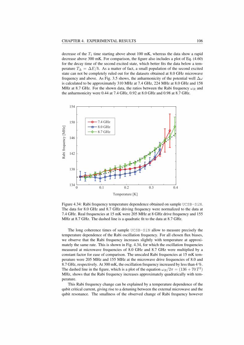
CHAPTER 4. EXPERIMENTAL RESULTS 106
decrease of the T1 time starting above about 100 mK, whereas the data show a rapiddecrease above 300 mK. For comparison, the figure also includes a plot of Eq. (4.60)for the decay time of the second excited state, which better fits the data below a tem-perature T∆ = ∆E/~. As a matter of fact, a small population of the second excitedstate can not be completely ruled out for the datasets obtained at 8.0 GHz microwavefrequency and above. As Fig. 3.5 shows, the anharmonicity of the potential well ∆ωis calculated to be approximately 310 MHz at 7.4 GHz, 224 MHz at 8.0 GHz and 158MHz at 8.7 GHz. For the shown data, the ratios between the Rabi frequency ωR andthe anharmonicity were 0.44 at 7.4 GHz, 0.92 at 8.0 GHz and 0.98 at 8.7 GHz.
0 0.1 0.2 0.3 0.4134
138
142
146
150
154
Temperature [K]
Rab
i fr
equ
ency
[M
Hz]
7.4 GHz
8.0 GHz
8.7 GHz
Figure 4.34: Rabi frequency temperature dependence obtained on sample UCSB-SiN.The data for 8.0 GHz and 8.7 GHz driving frequency were normalized to the data at7.4 GHz. Real frequencies at 15 mK were 205 MHz at 8 GHz drive frequency and 155MHz at 8.7 GHz. The dashed line is a quadratic fit to the data at 8.7 GHz.
The long coherence times of sample UCSB-SiN allow to measure precisely thetemperature dependence of the Rabi oscillation frequency. For all chosen flux biases,we observe that the Rabi frequency increases slightly with temperature at approxi-mately the same rate. This is shown in Fig. 4.34, for which the oscillation frequenciesmeasured at microwave frequencies of 8.0 GHz and 8.7 GHz were multiplied by aconstant factor for ease of comparison. The unscaled Rabi frequencies at 15 mK tem-perature were 205 MHz and 155 MHz at the microwave drive frequencies of 8.0 and8.7 GHz, respectively. At 300 mK, the oscillation frequency increased by less than 4 %.The dashed line in the figure, which is a plot of the equation ωR/2π = (136 + 70 T 2)MHz, shows that the Rabi frequency increases approximately quadratically with tem-perature.
This Rabi frequency change can be explained by a temperature dependence of thequbit critical current, giving rise to a detuning between the external microwave and thequbit resonance. The smallness of the observed change of Rabi frequency however
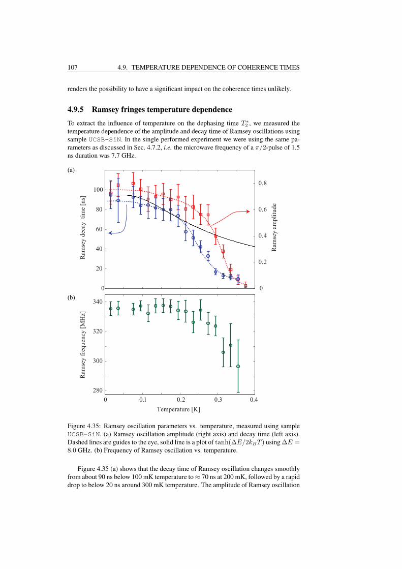
107 4.9. TEMPERATURE DEPENDENCE OF COHERENCE TIMES
renders the possibility to have a significant impact on the coherence times unlikely.
4.9.5 Ramsey fringes temperature dependence
To extract the influence of temperature on the dephasing time T ∗2 , we measured thetemperature dependence of the amplitude and decay time of Ramsey oscillations usingsample UCSB-SiN. In the single performed experiment we were using the same pa-rameters as discussed in Sec. 4.7.2, i.e. the microwave frequency of a π/2-pulse of 1.5ns duration was 7.7 GHz.
0 0.1 0.2 0.3 0.4
0
0.2
0.4
0.6
0.8
Temperature [K]
Ram
sey a
mpli
tude
0
20
40
60
80
100
Ram
sey d
ecay
ti
me
[ns]
280
300
320
340
Ram
sey f
requen
cy [
MH
z]
(a)
(b)
Figure 4.35: Ramsey oscillation parameters vs. temperature, measured using sampleUCSB-SiN. (a) Ramsey oscillation amplitude (right axis) and decay time (left axis).Dashed lines are guides to the eye, solid line is a plot of tanh(∆E/2kBT ) using ∆E =8.0 GHz. (b) Frequency of Ramsey oscillation vs. temperature.
Figure 4.35 (a) shows that the decay time of Ramsey oscillation changes smoothlyfrom about 90 ns below 100 mK temperature to≈ 70 ns at 200 mK, followed by a rapiddrop to below 20 ns around 300 mK temperature. The amplitude of Ramsey oscillation
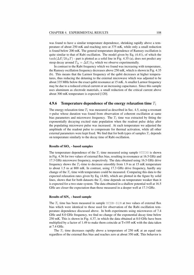
CHAPTER 4. EXPERIMENTAL RESULTS 108
was found to have a similar temperature dependence, shrinking rapidly above a tem-perature of about 250 mK and reaching zero at 375 mK, while only a small reductionis found below 200 mK. The general temperature dependence of Ramsey oscillation isquite similar to that of Rabi oscillation. The model given by Eq. (4.41), of which thetanh(∆E/2kBT ) - part is plotted as a solid line in Fig. 4.35 (a), does not predict anysteep decay around T∆ = ∆E/kB which we observe experimentally.
In contrast to the Rabi frequency which we found was increasing with temperature,the Ramsey oscillation frequency decreases above 250 mK, which is shown in Fig. 4.35(b). This means that the Larmor frequency of the qubit decreases at higher tempera-tures, thus reducing the detuning to the external microwave which was adjusted to beabout 335 MHz below the exact qubit resonance at 15 mK. A smaller Larmor frequencymay be due to a reduced critical current or an increasing capacitance. Since this sampleuses aluminum as electrode materials, a small reduction of the critical current aboveabout 300 mK temperature is expected [120].
4.9.6 Temperature dependence of the energy relaxation time T1
The energy relaxation time T1 was measured as described in Sec. 4.5, using a resonantπ-pulse whose duration was found from observation of coherent oscillation at samebias parameters and microwave frequency. The T1 time was extracted by fitting theexponentially decaying excited state population when the readout pulse delay afterthe populating microwave pulse was increased. At each temperature we adjusted theamplitude of the readout pulse to compensate for thermal activation, while all otherexternal parameters were kept fixed. We find that for both types of samples T1 dependson temperature similarly to the decay time of Rabi oscillation.
Results of SiOx - based samples
The temperature dependence of the T1 time measured using sample VTT30 is shownin Fig. 4.36 for two values of external flux bias, resulting in resonance at 16.5 GHz and17.3 GHz microwave frequency, respectively. The data obtained using 16.5 GHz drivefrequency shows the T1-time to decrease smoothly from 1.9 ns at 15 mK temperatureto about 1.5 ns at 800 mK. In contrast, using 17.3 GHz drive frequency, hardly anychange of the T1 time with temperature could be measured. Comparing this data to theexpected relaxation rates given by Eq. (4.60), which are plotted in the figure by solidlines, shows that for both datasets the T1-time depends on temperature weaker than itis expected for a two-state system. The data obtained in a shallow potential well at 16.5GHz are closer the expectation than those measured in a deeper well at 17.3 GHz.
Results of SiNx - based sample
The T1 time has been measured in sample UCSB-SiN at two values of external fluxbias which were identical to those used for observation of the Rabi oscillation tem-perature dependence discussed above. In both experiments using microwaves of 7.4GHz and 8.0 GHz frequency, we find no change of the exponential decay time below250 mK. This is shown in Fig. 4.37, in which the data obtained at 8.0 GHz have beenmultiplied by a factor of 1.49 to make them coincide at T=195 mK with the data takenat 7.4 GHz.
The T1 time decreases rapidly above a temperature of 250 mK at an equal rateregardless of the external flux bias and reaches zero at about 350 mK. This behavior is
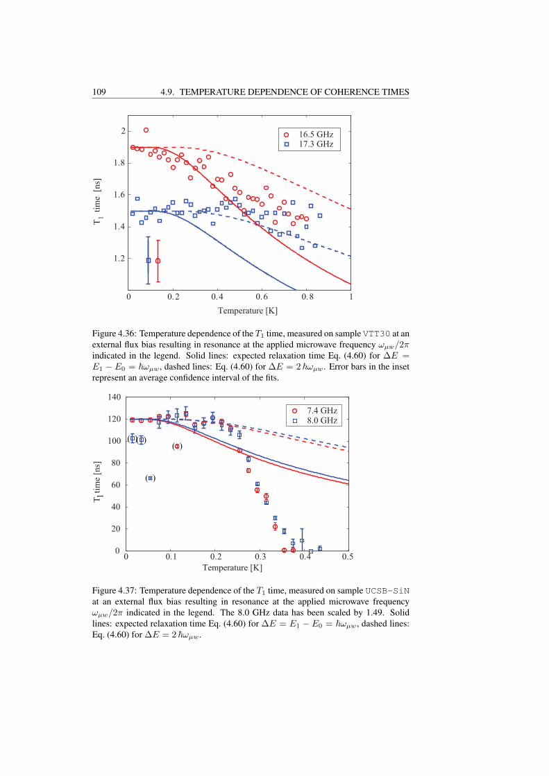
109 4.9. TEMPERATURE DEPENDENCE OF COHERENCE TIMES
0 0.2 0.4 0.6 0.8 1
1.2
1.4
1.6
1.8
2
Temperature [K]
T1
tim
e [
ns]
16.5 GHz17.3 GHz
Figure 4.36: Temperature dependence of the T1 time, measured on sample VTT30 at anexternal flux bias resulting in resonance at the applied microwave frequency ωµw/2πindicated in the legend. Solid lines: expected relaxation time Eq. (4.60) for ∆E =E1 − E0 = ~ωµw, dashed lines: Eq. (4.60) for ∆E = 2 ~ωµw. Error bars in the insetrepresent an average confidence interval of the fits.
0 0.1 0.2 0.3 0.4 0.50
20
40
60
80
100
120
140
Temperature [K]
T1 t
ime
[ns]
7.4 GHz8.0 GHz
( )
( )( )( )
Figure 4.37: Temperature dependence of the T1 time, measured on sample UCSB-SiNat an external flux bias resulting in resonance at the applied microwave frequencyωµw/2π indicated in the legend. The 8.0 GHz data has been scaled by 1.49. Solidlines: expected relaxation time Eq. (4.60) for ∆E = E1 − E0 = ~ωµw, dashed lines:Eq. (4.60) for ∆E = 2 ~ωµw.
CHAPTER 4. EXPERIMENTAL RESULTS 110
very similar to the Rabi oscillation data taken at the same bias parameters. Accordingly,the expected temperature dependence of the relaxation time Eq. (4.60) does not fit thedata.
4.10 ConclusionsIn this section, we present the results of a systematic study of the temperature depen-dence of coherence times in phase qubits. In order to avoid thermal activation, at highertemperatures it is necessary to operate the qubit in a deep potential well. As this reducesthe anharmonicity of the well, parasitic population of higher excited states can only beavoided for small drive amplitude and, accordingly, small Rabi frequency. Since ourNb/SiOx - based samples have short coherence times of below 8 ns, we must drive themstrongly to allow for observation of several periods of the Rabi oscillation before de-coherence occurs. Therefore, these qubits were operated in the multi-level limit usingthe deep potential well required at higher temperatures. In contrast, the qubit samplewhich was made using SiNx as a dielectric could be operated in the two-state quantumlimit also at higher temperature. This is due to its much longer coherence time of about100 ns.
We observed semi-classical Rabi-like oscillations in samples operated in the multi-level limit up to temperatures of 900 mK. Hereby, a loss of contrast due to thermalactivation in the detector dc SQUID is avoided by a newly implemented data evalua-tion procedure which is based on weighted fitting of the switching-current distribution.A systematic evaluation of the temperature dependence of the Rabi-like oscillation am-plitude and decay time shows that these values depend only weakly on temperature insamples operated in the multi-level limit. The same is true for the temperature depen-dence of the T1 time.
The Al/SiNx-sample which was operated in the two-level quantum limit showed aqualitatively different temperature dependence. The T1 time, the decay time of Rabioscillations and the T ∗2 time, which was measured from a Ramsey fringe experiment,altogether rapidly decrease close to the temperature where the thermal energy kBT isequal to the energy difference ∆E of the two qubit states. Below this temperature,which for the used samples was ≈ 400 mK, the coherence times depend only weaklyon temperature. The Rabi oscillation amplitude in contrast showed a particular non-monotonic temperature dependence when the qubit was operated in very deep potentialwells.
These peculiar results do not agree with the temperature dependence which is ex-pected from models describing thermal population of the excited state and taking intoaccount accelerated relaxation at higher temperatures. These models predict a strongertemperature dependence of decoherence for low temperatures. The rapid decrease ofcoherence time, which was observed in the sample operated in the two-level limit whenkBT ≈ ∆E, also is not expected from these models.
We speculate that, at low temperatures, qubit coherence is limited by a mecha-nism which gets less effective at higher temperatures. Such a mechanism could bethe coupling of the qubit to a bath of two-level fluctuators, which saturate at highertemperatures.

Summary
In this thesis, the coherent dynamics of superconducting phase quantum bits (qubits)are studied. A flux-biased phase qubit consists of a superconducting loop which is in-terrupted by a Josephson junction. The single degree of freedom of such a device is thephase difference ϕ of the superconducting order parameter across the junction, whichdepends on the magnetic flux threading the loop. As the logical states, a phase qubituses two eigenstates of the Josephson phase ϕ which are kept confined in a metastablepotential well. An externally applied magnetic flux is used to control the energy differ-ence between the two qubit states.
I describe the phase qubit principles and designs of samples which were fabri-cated using a standard commercial photolithographic process. These samples weresuccessfully operated in the quantum regime, demonstrating coherent qubit control bymicrowave and dc flux pulses.
The experimental methods required to operate phase qubits in the coherent quan-tum regime are discussed. For qubit readout, we implement a technique which is basedon the application of a short magnetic flux pulse. It reaches a contrast close to 100%,which is limited only at higher temperatures by thermal activation occurring duringthe readout pulse. Microwave spectroscopy was used to characterize the energy levelstructure of the samples. For strong driving, we observed transitions to higher ex-cited qubit states induced by multi-photon absorption processes. We evaluate the qubitcoherence time T ′2 by analyzing the resonance peak width dependence of microwavepower. These experiments indicate the existence of decoherence sources which giverise to inhomogeneous resonance broadening.
A prominent source of phase qubit decoherence is energy relaxation, which wemeasure directly by observing the exponential decay of the excited state. The samplesfabricated in standard technology had T1 decay times of less than 8 ns. Short coherencetimes in this type of qubits are due to a coupling of the qubit to a large number of two-level fluctuators which reside in the oxide dielectrics used in junction fabrication. Thisis confirmed by our measurements on a sample which was made using SiNx dielectric,showing a much longer T1 time of about 100 ns.
Logical operations on the phase qubit are accomplished by resonant interactionwith an applied microwave field, inducing coherent Rabi oscillation between the energylevels. We observe these oscillations in the time domain by driving the qubits withmicrowave pulses of varying duration. In standard samples fabricated using SiO2-dielectric, the oscillations decay after a mean time of about 3 - 5 ns. In the SiNx-basedsample, we observe Rabi oscillation decay times of about 100 ns, in agreement withindependent measurements of the UCSB group. This confirms that the noise level in
111

SUMMARY 112
our experimental setup is low enough not to affect the coherent dynamics on the studiedtime scale.
For weakly driven qubits, the Rabi frequency depends linearly on drive amplitude,as expected. At strong driving, we find a saturation of the oscillation frequency at avalue which is close to the anharmonicity of the qubit potential well, which indicatesthat higher excited states are taking part in coherent oscillations.
Using the high quality SiNx-based sample, we demonstrate a Ramsey fringe ex-periment and characterize qubit decoherence caused by dephasing. In agreement withindependent measurements, we find a dephasing time of T ∗2 ≈ 90 ns, which indicatesthat no significant sources of low-frequency noise exist in our experimental setup. Ina similar experiment, we demonstrate an implementation of the phase gate which isbased on the application of a short detuning flux bias pulse. This technique will beuseful for qubit state tomography.
We performed a first systematic study of the temperature dependence of coherencetimes in phase qubits. In order to avoid thermal activation, at higher temperatures itis necessary to operate the qubit in a deep potential well. As this reduces the anhar-monicity of the well, parasitic population of higher excited states can only be avoidedfor small drive amplitude and, accordingly, small Rabi frequency. Since our Nb/SiOx-based samples have short coherence times of below 8 ns, we must drive them stronglyfor observation of several periods of the Rabi oscillation. Therefore, these qubits wereoperated in the multi-level limit using the deep potential wells required at higher tem-peratures. In contrast, the qubit sample which was made using SiNx as a dielectriccould be operated in the two-state quantum limit also at high temperature due to itslong coherence time.
Semi-classical Rabi-like oscillations were observed in samples operated in the multi-level limit up to temperatures of 900 mK. Hereby, a loss of contrast due to thermal ac-tivation in the detector dc SQUID is avoided by a newly implemented data evaluationprocedure which is based on weighted fitting of the switching-current distribution. Asystematic evaluation of the temperature dependence of the Rabi-like oscillation am-plitude and decay time shows that these values depend only weakly on temperature insamples operated in the multi-level limit. A similar result was obtained for the temper-ature dependence of the T1 time.
In contrast, the Al/SiNx-sample which was operated in the two-level quantum limitshowed a qualitatively different temperature dependence. The T1 time, the decay timeof Rabi oscillations and the T ∗2 time, which was measured from a Ramsey fringe exper-iment, altogether rapidly decrease close to the temperature where the thermal energykBT is equal to the energy difference ∆E of the two qubit states. Below this tem-perature, which for the used sample was ≈ 400 mK, the coherence times depend onlyweakly on temperature. The Rabi oscillation amplitude in contrast showed a particularnon-monotonic temperature dependence when the qubit was operated in very deep po-tential wells.These striking new results remain to be analyzed by theoretical models dealing withmechanisms that cause decoherence in superconducting Josephson junction qubits. Ourexperimental results also suggest that currently existing qubits can be operated at muchhigher temperatures than those reported till now, without degrading already achievedcoherence times.

Zusammenfassung
Diese Dissertation fasst die Ergebnisse einer Untersuchung der quantenkoharentenZeitentwicklung von supraleitenden Phasen-Quantenbits (Qubits) zusammen. Diesebestehen aus einer supraleitenden Schleife, die durch einen kleinen Josephson-Kontaktunterbrochen ist. Der einzige Freiheitsgrad eines solchen Systems ist die Phasendif-ferenz ϕ des supraleitenden Ordnungsparameters uber dem Kontakt, welche vom mag-netischen Fluss durch die Schleife abhangt. Ein Phasenqubit verwendet als logischeZustande zwei Eigenzustande der Josephson-Phase ϕ, wobei diese auf eine metasta-bile Potentialmulde beschrankt werden. Die Energiedifferenz zwischen den beidenZustanden des Qubits wird durch einen angelegten magnetischen Fluss kontrolliert.
Ich beschreibe die Grundlagen des Phasen-Qubits und stelle das Design der Probenvor, welche mittels eines standardisierten photolithographischen Verfahrens kommer-ziell hergestellt wurden. Diese Proben wurden erfolgreich im Quantenregime be-trieben, wobei die Manipulation des Qubitzustandes mittels Mikrowellen- und Mag-netfeldpulsen demonstriert wurde.
Es werden die zum Betrieb von Phasen-Qubits im koharenten Quantenregime not-wendigen experimentellen Methoden dargelegt. Zum Auslesen des Qubits verwendenwir ein Verfahren, welches auf der Erzeugung eines kurzen Magnetfeldpulses basiert.Gemaß einer numerischen Untersuchung dieses Verfahrens erwarten wir eine hoheAuslesegenauigkeit von nahezu 100 %, die lediglich bei hohen Temperaturen durchthermische Aktivierung wahrend der Dauer des Magnetfeldpulses begrenzt wird.
Wir charakterisieren die Struktur der Energieniveaus der Proben mittels Mikrow-ellenspektroskopie. Im Fall großer Mikrowellenamplituden beobachten wir Ubergangezu hoher angeregten Qubitzustanden, welche durch Mehrphotonenabsorption entste-hen. Wir haben die Koharenzzeit T ′2 der Proben durch eine Analyse der Abhangigkeitder Resonanzlinienbreite von der Mikrowellenamplitude bestimmt. Diese Experimentedeuten darauf hin, dass in den getesteten standard-Qubits die Ursache der Dekoharenzauch zu inhomogener Resonanzlinienverbreiterung fuhrt.
Die hauptsachliche Ursache von Dekoharenz bei Phasen-Qubits ist Energierelax-ation. Diese fuhrt zum Zerfall des angeregten Qubitzustandes, welchen wir im zeitlichenVerlauf direkt beobachten. Die in standardisierten Prozessen hergestellten Qubits zeigteneine Zerfallszeit T1 von weniger als 8 ns. Solch kurze Koharenzzeiten sind in diesenProben bedingt durch die Kopplung des Qubits an eine grosse Zahl von zwei-NiveauZustanden, welche im SiO2-Dielektrikum des Josephson-Kontaktes bestehen. Dieswurde durch unsere Messungen an einem Qubit bestatigt, welches in einem speziellenProzess unter Verwendung eines SiNx-Dielektrikums hergestellt wurde und entsprech-end lange Koharenzzeiten von T1 ≈ 100 ns zeigt.
113

ZUSAMMENFASSUNG 114
Logische Qubit-Operationen werden durch resonante Wechselwirkung mit einemangelegten Mikrowellenfeld erreicht, die zur Erzeugung von Rabi-Oszillationen in derBesetzung der Energieniveaus fuhrt. Wir beobachten diese Oszillationen im zeitlichenVerlauf unter Verwendung eines Mikrowellenpulses variabler Dauer. In herkommlichenProben, die unter Verwendung eines SiO2-Dielektrikums hergestellt wurden, zeigendiese Oszillationen eine Abklingzeit von 3 bis 5 ns. In den Proben, die auf SiNx-Dielektrikum basieren, beobachten wir Abklingzeiten der Rabi-Oszillation von etwa100 ns in Ubereinstimmung mit unabhangigen Messungen. Dieses Ergebnis bestatigt,dass der Rauschpegel unseres experimentellen Aufbaus niedrig genug ist, um die ko-harente Qubit-Dynamik auf einer Zeitskala von 100 ns nicht zu beeintrachtigen.
Bei kleiner angelegter Mikrowellenleistung messen wir die erwartete lineare Ab-hangigkeit der Rabi-Frequenz von der Amplitude der Anregung. Bei hoheren Leistun-gen beobachten wir eine Sattigung der Oszillationsfrequenz bei einem Wert nahe derAnharmonizitat der die Qubitzustande enthaltenden Potentialmulde. Dies deutet da-rauf hin, dass bei diesen Leistungen hohere Qubitzustande angeregt werden und an derkoharenten Oszillation teilnehmen.
Unter Verwendung des hochwertigen, auf SiNx-basierenden Qubits demonstrierenwir ein Experiment zur Messung von Ramsey-Oszillationen, welches erlaubt, den An-teil von Dephasierung an der Dekoharenz zu bestimmen. In Ubereinstimmung mit un-abhangigen Messungen beobachten wir eine Dephasierungszeit von T ∗2 ≈ 90 ns, wasdarauf schliessen lasst, dass in unserem experimentellen Aufbau keine signifikantenQuellen von niederfrequentem Rauschen vorhanden sind. In einem ahnlichen Experi-ment zeigen wir die Realisierung des Phasengatters, welches auf der Erzeugung eineskurzen Magnetfeldpulses zur Verstimmung des Qubits basiert. Diese Methode wirdsich fur tomographische Messungen des Qubitzustandes als nutzlich erweisen.
Wir prasentieren die erste systematische Untersuchung der Temperaturabhangigkeitder Koharenzzeiten in Phasenqubits. Bei hohen Temperaturen muss thermische Ak-tivierung dadurch vermieden werden, dass das Qubit in einer tiefen Potentialmulde be-trieben wird. Da dies die Anharmonizitat der Potentialmulde verkleinert, kann eineungewunschte Anregung hoher Qubitzustande nur bei kleiner Anregungsamplitudeund enstprechend kleiner Rabi-Frequenz vermieden werden. Da unsere auf Nb/SiOx-basierenden Proben sehr kurze Koharenzzeiten von weniger als 8 ns haben, ist esnotwendig, diese mit hoher Anregungsamplitude zu betreiben, um einige Perioden derRabi-Oszillation beobachten zu konnen. Es ist deshalb unmoglich, diese Proben alsZweiniveausystem in den bei hohen Temperaturen notwendigen tiefen Potentialmuldenzu betreiben. Im Unterschied dazu ist es moglich, die uber ein Dielektrikum aus SiNx
verfugende Probe auch bei hoheren Temperaturen im Zweiniveau-Quantenlimit zu be-treiben.
Unter Verwendung der als Mehrniveausystem betriebenen Proben konnten wir semi-klassische Oszillationen, welche Rabioszillationen ahneln, bis zu einer maximalenTemperatur von 900 mK beobachten. Hierbei konnte eine Abnahme des Messkon-trastes aufgrund von thermischer Aktivierung im Detektor-DC-SQUID durch eine neuar-tige Methode der Datenauswertung vermieden werden, welche auf einer Regression-sanalyse der Schaltstrom-Wahrscheinlichkeitsverteilung basiert. Eine systematischeAuswertung der Temperaturabhangigkeiten von Amplitude und Abklingzeit der semik-lassischen Oszillationen sowie der Lebenszeit des angeregten Zustandes T1 erbrachte,dass diese Werte nur schwach von der Temperatur abhangen.
Im Gegensatz hierzu zeigt die als Zweiniveau-System betriebene Probe eine quali-tativ unterschiedliche Temperaturabhangigkeit. Die T1-Zeit, die Abklingzeit der Rabi-
115
Oszillation als auch die Abklingzeit T ∗2 der Ramsey-Oszillation nahmen schnell absobald die Probentemperatur einen Wert erreichte, bei dem die thermische Energy kBTgleich der Energiedifferenz ∆E zwischen den beiden Qubitzustanden ist. Unterhalbdieser Temperatur, welche fur die verwendete Probe bei ca. 400 mK liegt, hangen dieKoharenzzeiten nur schwach von der Temperatur ab.
Diese bemerkenswerten neuen Ergebnisse mussen in theoretischen Modellen Be-rucksichtigung finden, die die Dekoharenz von auf Josephson-Kontakten basieren-den Qubits beschreiben. Unsere Experimente zeigen daruber hinaus, dass momentanverfugbare Qubits bei sehr viel hoheren Temperaturen betrieben werden konnen als esbisher bekannt war.

ZUSAMMENFASSUNG 116
Bibliography
[1] E. Schrodinger, Naturwissenschaften 48, 49, 50, 807, 823, 844 (1935).
[2] R. Voss and R. Webb, Phys. Rev. Lett. 47, 265 (1981).
[3] M. Devoret, J. Martinis, and J. Clarke, Phys. Rev. Lett. 55, 1908 (1985).
[4] J. M. Martinis, M. H. Devoret, and J. Clarke, Phys. Rev. Lett. 55, 1543 (1985).
[5] M. H. Devoret, D. Esteve, and J. M. Martinis, Phys. Rev. B 36, 58 (1987).
[6] J. E. Mooij, T. P. Orlando, L. Levitov, L. Tian, C. H. van der Wal, and S. Lloyd,Science 285, 1036 (1999).
[7] J. R. Friedman, V. Patel, W. Chen, S. K. Tolpygo, and J. E. Lukens, nature 406,43 (2000).
[8] A. Barone and G. Paterno, Physics and Applications of the Josephson Effect(Wiley, New York, 1982).
[9] J. Clarke and A. Braginski, SQUID Handbook, vol. 1 (WILEY-VCH, 2004).
[10] J. Martinis, S. Nam, J. Aumentado, and C. Urbina, Phys. Rev. Lett. 89, 117901(2002).
[11] I. Chiorescu, Y. Nakamura, C. J. Harmans, and J. E. Mooij, Science 299, 186(2003).
[12] Y. Nakamura, Y. A. Pashkin, and J. S. Tsai, nature 398, 786 (1999).
[13] D. Vion, A. Aassime, A. Cottet, P. Joyez, H. Pothier, C. Urbina, D. Esteve, andM. Devoret, Science 296, 286 (2002).
[14] Hypres Inc., Elmsford, NY 10523, U.S.A.
[15] A. Steane, quant-ph/9708022 (1997).
[16] E. Rieffel and W. Polak, quant-ph/9809016 (1998).
[17] R. Feynman, Int. J. Theor. Phys. 21 (1982).
[18] D. Deutsch, Proc. R. Soc. Lond. 400, 97 (1985).
[19] M. A. Nielsen and I. L. Chuang, Quantum Computation and Quantum Informa-tion (Cambridge University Press, 2000).
117
BIBLIOGRAPHY 118
[20] R. Hughes et. al., A quantum information science and technology roadmap(2004), http://qist.lanl.gov/qcomp map.shtml.
[21] D. P. DiVincenzo, Fortschritte der Physik 48, 771 (2000),http://arxiv.org/abs/quant-ph/0002077.
[22] K. Likharev and V. Semenov, IEEE Trans. Appl. Supercond. 1, 3 (1991).
[23] S. O. Valenzuela, W. D. Oliver, D. M. Berns, K. K. Berggren, L. S. Levitov, andT. P. Orlando, Science 314, 1589 (2006).
[24] P. Shor, Phys. Rev. A 52, 2493 (1995).
[25] A. Steane, Phys. Rev. Lett. 77, 793 (1996).
[26] R. C. Bialczak, R. McDermott, M. Ansmann, M. Hofheinz, N. Katz,E. Lucero, M. Neeley, A. D. O’Connell, H. Wang, A. N. Cle-land, et al., 1/f flux noise in josephson phase qubits (2007),http://www.citebase.org/abstract?id=oai:arXiv.org:0708.2125.
[27] R. Simmonds, K. Lang, D. A. Hite, S. Nam, D. P. Pappas, and J. Martinis, Phys.Rev. Lett. 93, 0770031 (2004).
[28] S. Lloyd, Phys. Rev. Lett. 75, 346 (1995).
[29] R. McDermott, R. W. Simmonds, M. Steffen, K. B. Cooper, K. Cicak, K. D.Osborn, S. Oh, D. P. Pappas, and J. M. Martinis, Science 307, 1299 (2005).
[30] J. Clarke, T. L. Robertson, B. Plourde, A. Garcıa-Martinez, P. Reichardt, D. V.Harlingen, B. Chesca, R. Kleiner, Y. Makhlin, G. Schon, et al., Physica ScriptaT102, 173 (2002).
[31] T. Filippov, S. Tolpygo, J. Mannik, and J. Lukens, IEEE Trans. Appl. Supercond.13, 1005 (2003).
[32] M. G. Castellano, F. Chiarello, R. Leoni, D. Simeone, G. Torrioli, C. Cosmelli,and P. Carelli, Applied Physics Letters 86, 152504 (2005).
[33] A. Blais, A. M. van den Brink, and A. M. Zagoskin, Phys. Rev. Lett. 12, 127901(2003).
[34] K. B. Cooper, M. Steffen, R. McDermott, R. Simmonds, S. Oh, D. Hite, D. Pap-pas, and J. Martinis, Phys. Rev. Lett. 93, 180401 (2004).
[35] J. Lisenfeld, Probing quantum states in josephson junctions by microwaves(2003), diploma thesis, Friedrich-Alexander Universitat Erlangen-Nurnberg.
[36] J. Claudon, F. Balestro, F. Hekking, and O. Buisson, Phys. Rev. Lett. 93, 187003(2004).
[37] B. Josephson, Phys. Lett. 1, 251 (1962).
[38] W. C. Stewart, Appl. Phys. Lett 12, 277 (1968).
[39] D. E. McCumber, J. Appl. Phys. 39, 3113 (1968).
[40] M. Weihnacht, Phys. Stat. Sol. 32, K169 (1969).
119 BIBLIOGRAPHY
[41] M. Devoret, D. Esteve, and C. Urbina, Macroscopic Quantum Effects inthe Current-Biased Josephson Junction (Elsevier Science Publishers, 1992),chap. 6.
[42] M. Devoret, J. M. Martinis, D. Esteve, and J. Clarke, Phys. Rev. Lett. 53, 1260(1984).
[43] J. E. Marchese, M. Cirillo, and N. Grønbech-Jensen, Europ. Phys. Journ. onSpecial Topics 147, 333 (Aug. 2007), arXiv:0708.3701.
[44] M. V. Fistul and A. V. Ustinov, Phys. Rev. B 63, 024508 (2000).
[45] L. D. Landau and E. M. Lifschitz, Mechanik (Akademie-Verlag Berlin, 1976).
[46] A. Wallraff, T. Duty, A. Lukashenko, and A. V. Ustinov, Phys. Rev. Lett. 90,370031 (2003).
[47] H. A. Kramers, Physica 7, 284 (1940).
[48] H. Grabert, P. Olschowski, and U. Weiss, Phys. Rev. B 36, 1931 (1987).
[49] M. Buttiker, E. Harris, and R. Landauer, Phys. Rev. B 28, 1268 (1983).
[50] K. K. Likharev, Dynamics of Josephson junctions and circuits (Gordon andBreach Science, 1986).
[51] A. O. Caldeira and A. J. Leggett, Phys. Rev. Lett. 46, 211 (1981).
[52] A. O. Caldeira and A. J. Legget, Ann. of Phys. 149, 374 (1983).
[53] P. Silvestrini, V. G. Palmieri, B. Ruggiero, and M. Russo, Phys. Rev. Lett. 79,3046 (1997).
[54] I. Affleck, Phys. Rev. Lett. 46, 388 (1981).
[55] J. M. Martinis, M. H. Devoret, and J. Clarke, Phys. Rev. B 35, 4682 (1987).
[56] C. Cohen-Tannoudji, B. Diu, and F. Laloe, Quantum Mechanics, vol. 1 (Wiley-Interscience, 1977).
[57] S. Han, Y. Yang, and X. e. a. Chu, Science Magazine 293, 1457 (2001).
[58] J. M. Martinis, S. Nam, J. Aumentado, K. M. Lang, and C. Urbina, Phys. Rev.B. 67, 094510 (2003).
[59] C. H. van der Wal, A. C. J. ter Haar, F. K. Wilhelm, R. N. Schouten, C. Harmans,T. P. Orlando, S. Lloyd, and J. E. Mooij, Science 290, 773 (2000).
[60] T. L. Robertson, Fundamentals of Flux-based Quantum Computing, Ph.D. the-sis, University of California, Berkely (2005).
[61] R. Simmonds, D. Hite, R. McDermott, M. Steffen, K. Cooper, K. Lang, J. Marti-nis, and D. Pappas, Quantum Computation: solid state systems (Springer Verlag,Berlin, 2005), chap. Junction Materials Research using Phase Qubits.
[62] D. Esteve, M. H. Devoret, and J. M. Martinis, Phys. Rev. B 34, 158 (1986).

BIBLIOGRAPHY 120
[63] A. Berkley, A Josephson junction qubit, Ph.D. thesis, University of Maryland(2003).
[64] R. M. Lewis, H. Paik, S. K. Dutta, T. A. Palomaki, K. Mitra, B. K. Cooper,A. Przybysz, C. J. Anderson, J. R.and Lobb, and F. C. Wellstood, QuantumInformation and Computation IV (2006), vol. 6244 of Proceedings of the SPIE,chap. Some properties of a dc SQUID qubit.
[65] K. Lang, S. Nam, J. Aumentado, C. Urbina, and J. M. Martinis, IEEE Transac-tions on Applied Superconductivity 13, 2003 (2003).
[66] J. Zimmermann and A. Silver, Phys. Rev. 157, 317 (1967).
[67] A. G. Kofman, Q. Zang, J. M. Martinis, and A. N. Korotkov, Phys. Rev. B 75,014524 (2007).
[68] Q. Zhang, A. G. Kofman, J. Martinis, and A. N. Korotkov, Phys. Rev. B 74,2145181 (2006).
[69] R. Rouse, S. Han, and J. E. Lukens, Phys. Rev. Lett. 75, 1614 (Aug 1995).
[70] K. Likharev, Physica B p. 1079 (1981).
[71] V. Lefevre-Seguin, E. Turlot, C. Urbina, D. Esteve, and M. H. Devoret, Phys.Rev. B. 46, 5507 (1992).
[72] F. Chiarello, P. Carelli, M. G. Castellano, C. Cosmelli, L. Gangemi, R. Leoni,S. Poletto, D. Simeone, and G. Torrioli, Supercond. Sci. Tech. 18, 1370 (2005).
[73] V. Schmidt, P. Muller, and A. Ustinov, The Physics of Superconductors (SpringerVerlag Berlin, 1997).
[74] V. Lefevre-Seguin, E. Turlot, C. Urbina, D. Esteve, and M. Devoret, Phys. Rev.B 91, 5507 (1992).
[75] F. Balestro, J. Claudon, J. Pekola, and O. Buisson, Phys. Rev. Lett. 46, 158301(2003).
[76] C. van der Wal, F. Wilhelm, C. Harmans, and J. Mooij, Eur. Phys. J. B 31, 111(2003).
[77] T. A. Fulton and L. N. Dunkleberger, Phys. Rev. B 9, 4760 (1974).
[78] A. Wallraff, A. Lukashenko, C. Coqui, T. Duty, and A. V. Ustinov, Rev. Sci.Instr. 74, 3740 (2003).
[79] T. L. Robertson, B. L. T. Plourde, T. Hime, S. Linzen, P. A. Reichardt, F. K.Wilhelm, and J. Clarke, Phys. Rev. B 72, 024513 (2005).
[80] T. Hime, P. Reichardt, B. Plourde, T. Robertson, C.-E. Wu, A. Ustinov, andJ. Clarke, Science 314, 1427 (2006).
[81] VTT Technical Research Center, Finland.
[82] Whiteley Research Inc., Sunnyvale, CA 94086, U.S.A., FastHenry v3.0wr.

121 BIBLIOGRAPHY
[83] E. Il’ichev, N. Oukhanski, A. Izmalkov, T. Wagner, M. Grajcar, H.-G. Meyer,A. Y. Smirnov, A. M. van den Brink, M. H. S. Amin, and A. M. Zagoskin, Phys.Rev. Lett 91, 097906 (2003).
[84] M. Steffen, M. Ansmann, R. McDermott, N. Katz, R. Bialczak, E. Lucero,M. Neeley, E. Weig, A. Cleland, and J. Martinis, Phys. Rev. Lett. 97, 050502(2006).
[85] Aeroflex / Inmet Inc., Ann Arbor, MI 48103, U.S.A., http://www.aeroflex-inmet.com.
[86] Huber + Suhner GmbH, D-82024 Taufkirchen, Germany,http://www.hubersuhner.de.
[87] A. Lukashenko and A. V. Ustinov, to appear in Rev. Sci. Instr. (2007).
[88] Vacuumschmelze GmbH & Co. KG, D-63450 Hanau,http://www.vacuumschmelze.de.
[89] Texas Instruments, DAC714 datasheet, http://www-s.ti.com/sc/ds/dac714.pdf.
[90] Maxim Integrated Products, http://www.maxim-ic.com.
[91] Stanford Research Systems, SR 620 universal time interval counter.
[92] Y. S. Greenberg, A. Izmalkov, M. Grajcar, E. Il’ichev, W. Krech, and H.-G.Meyer, Phys. Rev. B 66, 224511 (2002).
[93] A. Lupascu, C. J. Verwijs, R. N. Schouten, C. J. Harmans, and J. E. Mooij, Phys.Rev. Lett. 93, 177006 (2004).
[94] The Mathworks Inc., http://www.mathworks.com.
[95] Marki Microwave Inc., M8-0420, http://www.markimicrowave.com.
[96] ARRA inc., power divider model 0200-2, http://www.arra.com/.
[97] D. Schwartz, B. Sen, C. Archie, and J. Lukens, Phys. Rev. Lett. 55, 1547 (1985).
[98] J. Kurkijarvi, Phys. Rev. B 6, 832 (1972).
[99] H. Grabert, P. Olschowski, and U. Weiss, Phys. Rev. B. 32, 2712 (1985).
[100] H. Grabert, P. Olschowski, and U. Weiss, Phys. Rev. Lett. 57, 265 (1986).
[101] R. McDermott, M. Steffen, M. Ansmann and J.M. Martinis, private communi-cation.
[102] F. Bloch, Phys. Rev. 70, 460 (1946).
[103] M. Goordon, Theory of Josephson persistent-current qubits with driving anddissipation, Master’s thesis, Delft University of Technology (2002).
[104] S. Saito, M. Thorwart, H. Tanaka, M. Ueda, H. Nakano, K. Semba, andH. Takayanagi, Phys. Rev. Lett. 93, 037001 (2004).
[105] Y. Nakamura, Y. A. Pashkin, and J. S. Tsai, Phys. Rev. Lett. 87, 246601 (2002).
BIBLIOGRAPHY 122
[106] A. Ratchov, Etude du couplage de petits systemes quantiques avec leur environ-nement: fluctutations et decoherence a basse temperature, Ph.D. thesis, Univer-site Joseph Fourier, Grenoble (2005).
[107] M. Weissman, Rev. Mod. Phys. 60, 537 (1988).
[108] A. Abragam, The Principles of Nuclear Magnetism (Oxford University Press,Glassgow, 1961).
[109] F. Bloch and A. Siegert, Phys. Rev. 57, 522 (1940).
[110] L. Ku and C. Yu, Phys. Rev. B 72, 024526 (2005).
[111] M. Amin, Low Temp. Phys. 32, 198 (2006).
[112] F. Meier and D. Loss, Phys. Rev. B 71, 094519 (2005).
[113] L. Tian and S. Lloyd, Phys. Rev. A 62, 050301 (2000).
[114] N. F. Ramsey, Phys. Rev. 78, 695 (1950).
[115] L. Tian, S. Lloyd, and T. Orlando, Phys. Rev. B 65, 144516 (2002).
[116] F. K. Wilhelm, M. J. Storcz, C. H. van der Wal, C. J. P. M. Harmans, and J. E.Mooij, Adv. Solid State Phys. 43, 763 (2003).
[117] A. Leggett, S. Chakravarty, A. Dorsey, M. Fisher, A. Garg, and W. Zwerger,Rev. Mod. Phys. 59, 1 (1987).
[118] M. Grifoni, E. Paladino, and U. Weiss, Eur. Phys. J. B 10, 719 (1999).
[119] C. Slichter, Principles of magnetic resonance (Springer Verlag, 1990).
[120] V. Ambegaokar and A. Baratoff, Phys. Rev. Lett. 10, 486 (1963).

List of Publications
• J. Lisenfeld, A. Lukashenko, and A.V. Ustinov, High-contrast readout of su-perconducting qubits beyond the single-shot resolution limit, to be published inAppl. Phys. Lett. (2007)
• J. Lisenfeld, A. Lukashenko, M. Ansmann, J. M. Martinis, and A.V. Ustinov,Temperature dependence of coherent oscillations in Josephson phase qubits,Phys. Rev. Lett. 99, 170504 (2007)
• X. Jin, J. Lisenfeld, Y. Koval, A. Lukashenko, A.V. Ustinov, and P. Muller, En-hanced Macroscopic Quantum Tunneling in Bi2Sr2CaCu2O8+δ Intrinsic Joseph-son Junction Stacks, Phys. Rev. Lett. 96, 177003 (2006)
• J. Lisenfeld, A. Lukashenko, and A.V. Ustinov, Macroscopic quantum coher-ence in rf-SQUIDs, Proceedings of the International Symposium on MesoscopicSuperconductivity and Spintronics, NTT R&D Center, Atsugi, Kanagawa, Japan(2006)
• B. Ivlev, G. Pepe, R. Latempa, A. Barone, F. Barkov, J. Lisenfeld, and A.V. Usti-nov, Extreme multiphoton phenomena in Josephson junctions: Euclidean reso-nance, Phys. Rev. B 72, 094507 (2005)
• A. Wallraff, A. Lukashenko, J. Lisenfeld, A. Kemp, M. Fistul, Y. Koval, andA.V. Ustinov, Quantutm dynamics of a single vortex, Nature 425, 155 (2003).
123