Experiments for Theorists
35
Experiments for Theorists Suzanne Staggs Chicago Spectrum Workshop; May 2015
Transcript of Experiments for Theorists

Experiments for Theorists Suzanne Staggs
Chicago Spectrum Workshop; May 2015

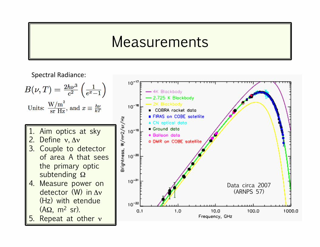
Measurements
Data circa 2007 (ARNPS 57)
Spectral Radiance:
More decades of frequency than Dale showed earlier
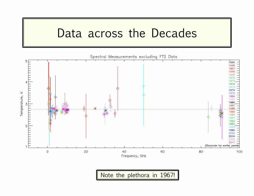
Data across the Decades
Note the plethora in 1967!
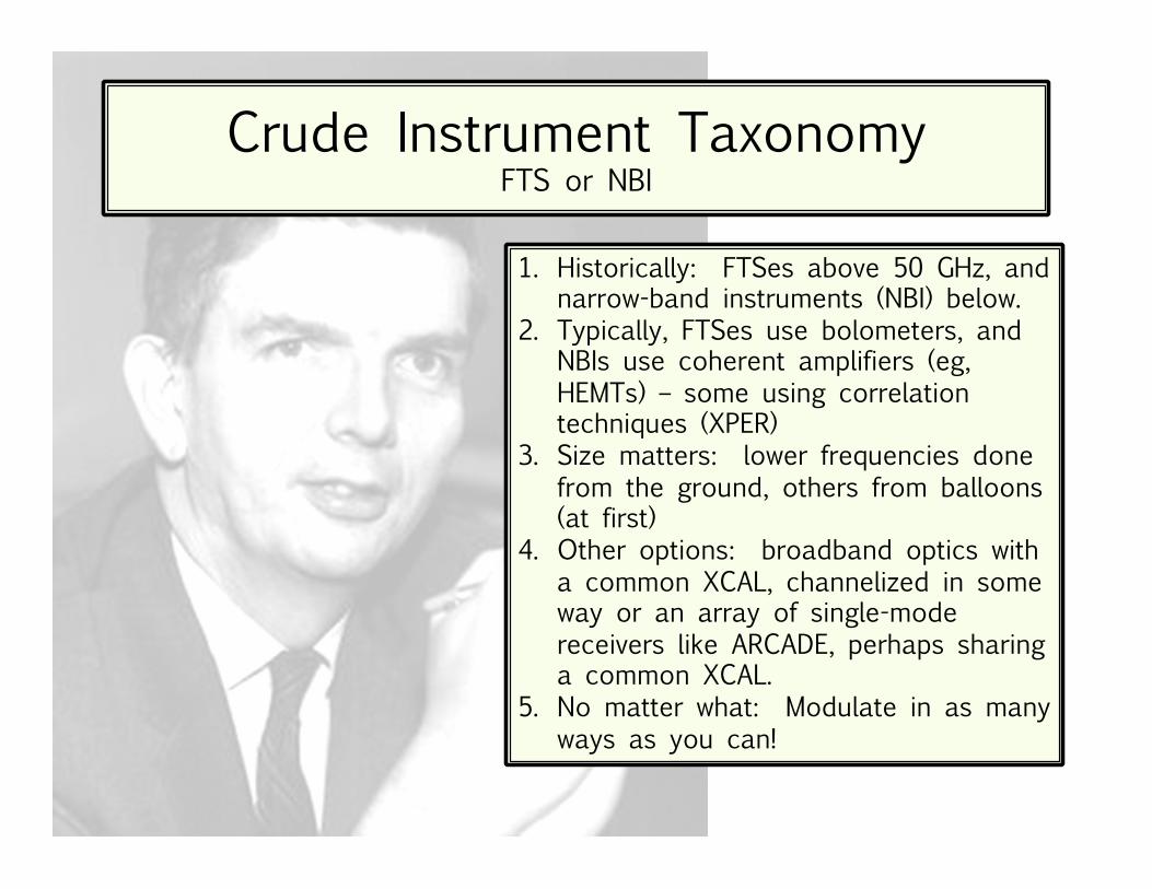
1. Historically: FTSes above 50 GHz, and narrow-band instruments (NBI) below.
2. Typically, FTSes use bolometers, and NBIs use coherent amplifiers (eg, HEMTs) – some using correlation techniques (XPER)
3. Size matters: lower frequencies done from the ground, others from balloons (at first)
4. Other options: broadband optics with a common XCAL, channelized in some way or an array of single-mode receivers like ARCADE, perhaps sharing a common XCAL.
5. No matter what: Modulate in as many ways as you can!
Crude Instrument Taxonomy FTS or NBI
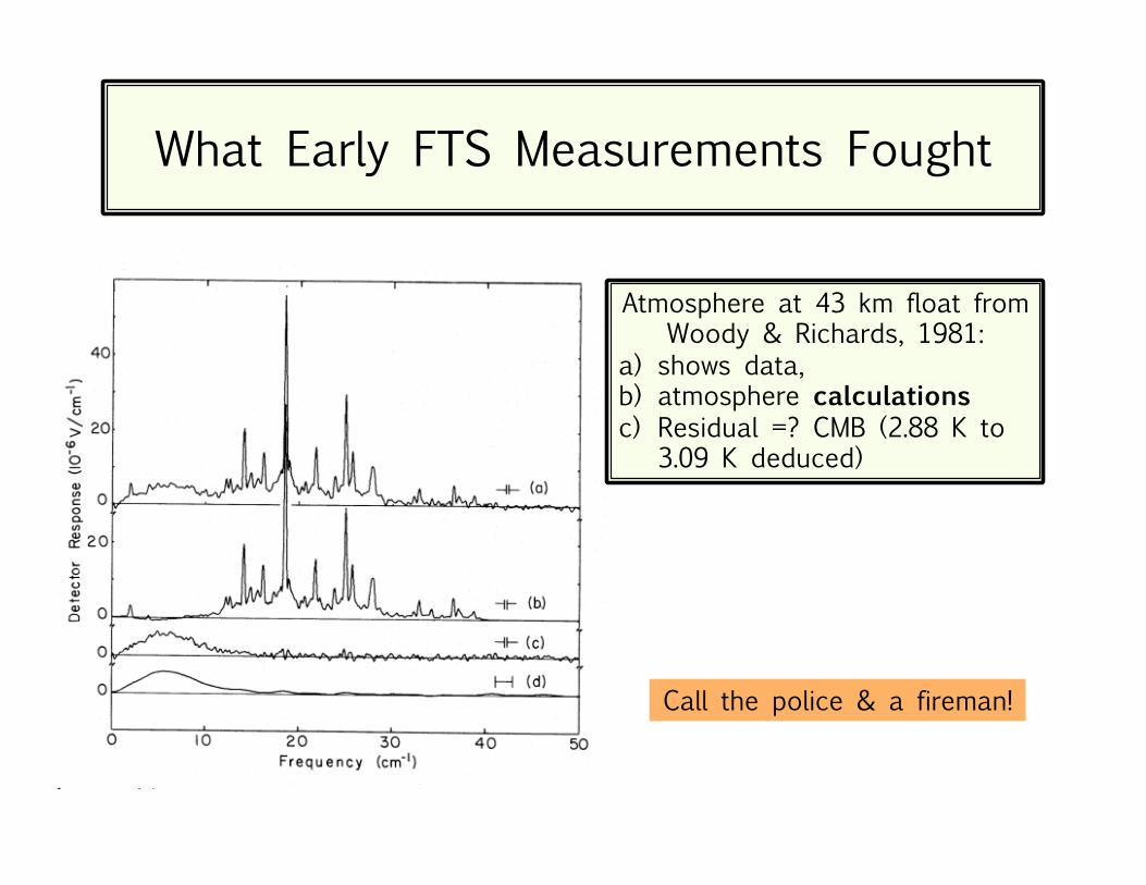
What Early FTS Measurements Fought
Atmosphere at 43 km float from Woody & Richards, 1981:
a) shows data, b) atmosphere calculations c) Residual =? CMB (2.88 K to
3.09 K deduced)
Call the police & a fireman!
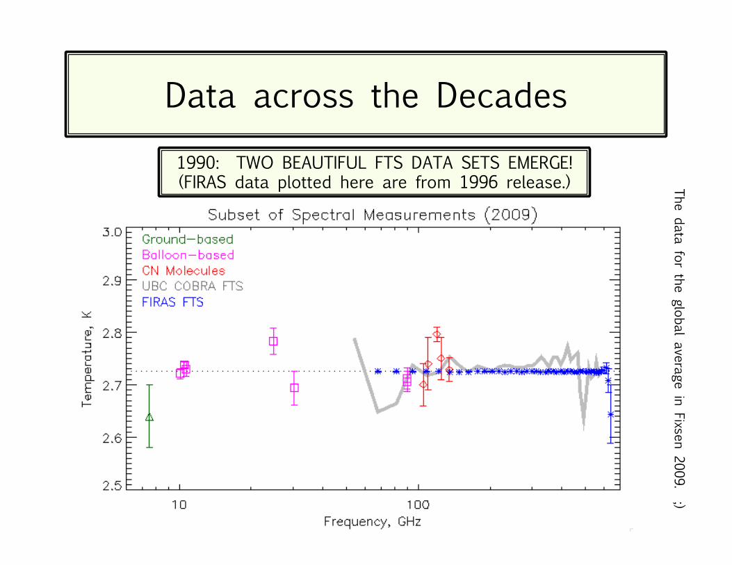
Data across the Decades The data for the global average in Fixsen 2009. ;)
1990: TWO BEAUTIFUL FTS DATA SETS EMERGE! (FIRAS data plotted here are from 1996 release.)
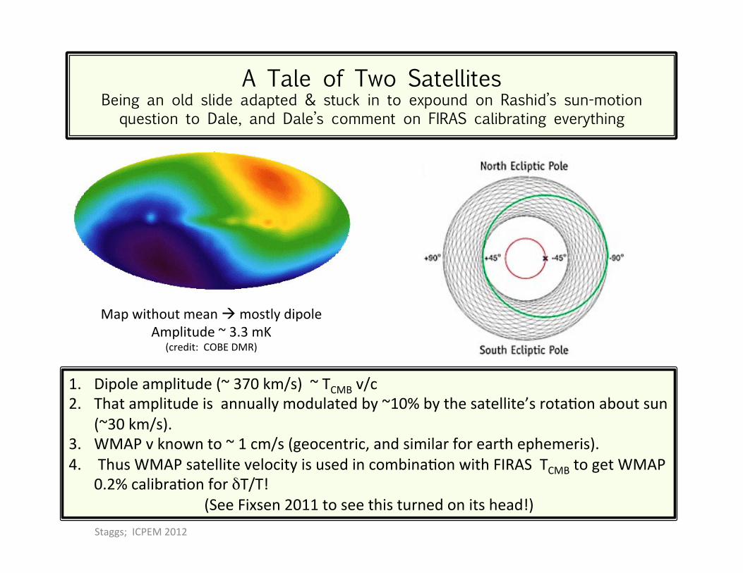
A Tale of Two Satellites Being an old slide adapted & stuck in to expound on Rashid’s sun-motion
question to Dale, and Dale’s comment on FIRAS calibrating everything
Map without mean à mostly dipole Amplitude ~ 3.3 mK
(credit: COBE DMR)
1. Dipole amplitude (~ 370 km/s) ~ TCMB v/c 2. That amplitude is annually modulated by ~10% by the satellite’s rotaNon about sun
(~30 km/s). 3. WMAP v known to ~ 1 cm/s (geocentric, and similar for earth ephemeris). 4. Thus WMAP satellite velocity is used in combinaNon with FIRAS TCMB to get WMAP
0.2% calibraNon for δT/T! (See Fixsen 2011 to see this turned on its head!)
Staggs; ICPEM 2012
Measurements
Data circa 2007 (ARNPS 57)
Spectral Radiance:
1. Aim optics at sky 2. Define ν, Δν 3. Couple to detector
of area A that sees the primary optic subtending Ω
4. Measure power on detector (W) in Δν (Hz) with etendue (AΩ, m2 sr).
5. Repeat at other ν

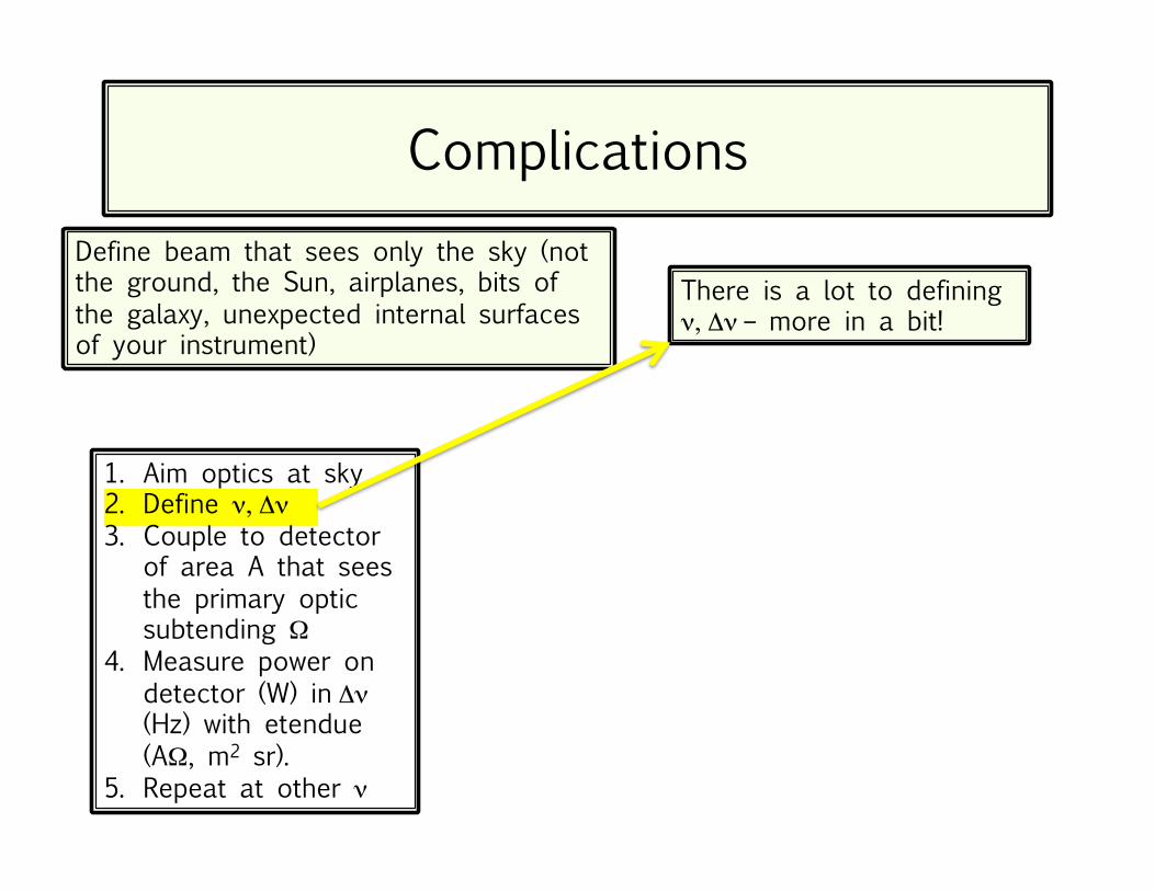
Complications
1. Aim optics at sky 2. Define ν, Δν 3. Couple to detector
of area A that sees the primary optic subtending Ω
4. Measure power on detector (W) in Δν (Hz) with etendue (AΩ, m2 sr).
5. Repeat at other ν
Define beam that sees only the sky (not the ground, the Sun, airplanes, bits of the galaxy, unexpected internal surfaces of your instrument)
1. Aim optics at sky 2. Define ν, Δν 3. Couple to detector
of area A that sees the primary optic subtending Ω
4. Measure power on detector (W) in Δν (Hz) with etendue (AΩ, m2 sr).
5. Repeat at other ν
Complications Define beam that sees only the sky (not the ground, the Sun, airplanes, bits of the galaxy, unexpected internal surfaces of your instrument)
There is a lot to defining ν, Δν – more in a bit!
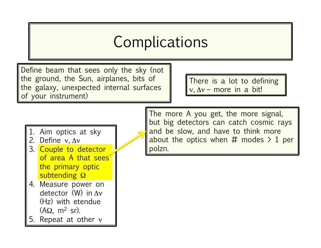
The more A you get, the more signal, but big detectors can catch cosmic rays and be slow, and have to think more about the optics when # modes > 1 per polzn.
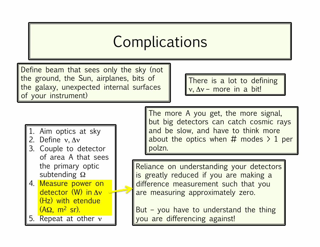
1. Aim optics at sky 2. Define ν, Δν 3. Couple to detector
of area A that sees the primary optic subtending Ω
4. Measure power on detector (W) in Δν (Hz) with etendue (AΩ, m2 sr).
5. Repeat at other ν
Complications Define beam that sees only the sky (not the ground, the Sun, airplanes, bits of the galaxy, unexpected internal surfaces of your instrument)
There is a lot to defining ν, Δν – more in a bit!
Reliance on understanding your detectors is greatly reduced if you are making a difference measurement such that you are measuring approximately zero. But – you have to understand the thing you are differencing against!
The more A you get, the more signal, but big detectors can catch cosmic rays and be slow, and have to think more about the optics when # modes > 1 per polzn.

Calibrations
1. Idea: compare to an extremely good blackbody (XCAL) at TCMB 2. The chicken and the egg: how do you know the XCAL is as
good as you need? a) Kirchoff helps – you can use precision instruments and
measure reflections from a hot source in the lab b) Griffiths, Born & Wolf & Jackson help too c) If you ask for too much, materials may let you down (eg, by
having unexpected resonances in their dielectric ‘constants’) 3. Borrowing a page from FIRAS: If you can parameterize the XCAL
deviations from perfection you can fit them out... (PIXIE 30 thermometers: yeah, baby!)
4. Note that a 3 nK distortion of unkown shape requires -90 dB! 5. Measure as much as you can in situ (eg, change its DC
temperature, force gradients, move it in and out, etc)
Frequencies
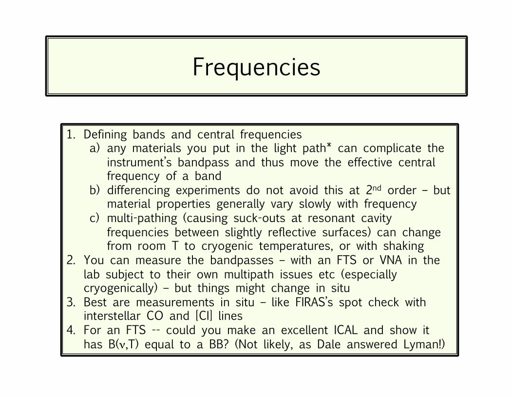
1. Defining bands and central frequencies a) any materials you put in the light path* can complicate the
instrument’s bandpass and thus move the effective central frequency of a band
b) differencing experiments do not avoid this at 2nd order – but material properties generally vary slowly with frequency
c) multi-pathing (causing suck-outs at resonant cavity frequencies between slightly reflective surfaces) can change from room T to cryogenic temperatures, or with shaking
2. You can measure the bandpasses – with an FTS or VNA in the lab subject to their own multipath issues etc (especially cryogenically) – but things might change in situ
3. Best are measurements in situ – like FIRAS’s spot check with interstellar CO and [CI] lines
4. For an FTS -- could you make an excellent ICAL and show it has B(ν,T) equal to a BB? (Not likely, as Dale answered Lyman!)
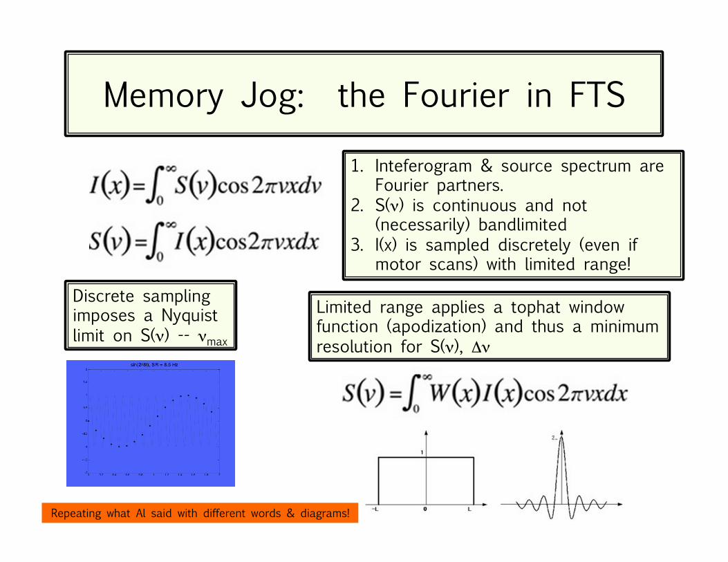
Memory Jog: the Fourier in FTS
1. Inteferogram & source spectrum are Fourier partners.
2. S(ν) is continuous and not (necessarily) bandlimited
3. I(x) is sampled discretely (even if motor scans) with limited range!
Discrete sampling imposes a Nyquist limit on S(ν) -- νmax
Limited range applies a tophat window function (apodization) and thus a minimum resolution for S(ν), Δν
Repeating what Al said with different words & diagrams!

PIXIE Apodization
Slide borrowed from Dale Fixsen’s Okinawa talk in 2012.

Detector Sensitivities
Converting between NEP (units W Hz-1/2) and NET (units mK s1/2)
To get power for a single mode: integrate over frequency and the etendue AΩ. For x <<1, and a tophat, eg: P = kTΔν
Note, for CMB, x=1 for ν=59 GHz. Also note, for small x nγ=(ex-1)-1 is large.
For x<<1, dP/dT = kΔν, independent of ν. In general,
Two last details: 1. There is a conversion
factor 2 between Hz-1 and s! The former implies sine waves and the latter square waves.
2. Need to account for instrument losses (throughput η<1).
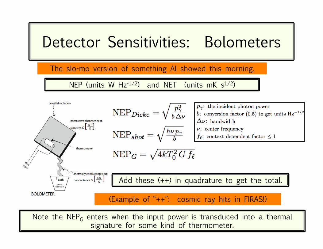
Detector Sensitivities: Bolometers
NEP (units W Hz-1/2) and NET (units mK s1/2)
Add these (++) in quadrature to get the total.
Note the NEPG enters when the input power is transduced into a thermal signature for some kind of thermometer.
(Example of “++”: cosmic ray hits in FIRAS!)
The slo-mo version of something Al showed this morning.
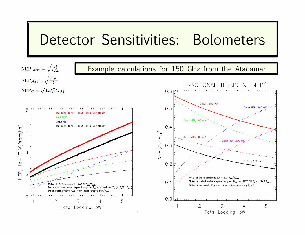
Detector Sensitivities: Bolometers
Example calculations for 150 GHz from the Atacama:
∝
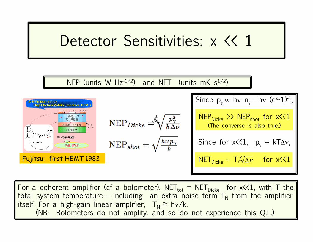
Detector Sensitivities: x << 1
NEP (units W Hz-1/2) and NET (units mK s1/2)
Fujitsu: first HEMT 1982
For a coherent amplifier (cf a bolometer), NETtot = NETDicke for x<<1, with T the total system temperature – including an extra noise term TN from the amplifier itself. For a high-gain linear amplifier, TN hν/k. (NB: Bolometers do not amplify, and so do not experience this Q.L.)
Since pγ hν nγ =hν (ex-1)-1,
NEPDicke >> NEPshot for x<<1 (The converse is also true.)
Since for x<<1, pγ ~ kTΔν,
NETDicke ~ T/ for x<<1
∝Δν
Δν
≥
≥

Detector Sensitivities: Coda I
NEP (units W Hz-1/2) and NET (units mK s1/2)
Radiometer Equation: δT = Tsys / (Δν )t
where δT is the error after t seconds of integration, and Tsys includes TN for coherent amplifiers, and where x<<1 (but remember x = x(T).)
If you want more – Caves, PRD 26, 1817 (1982) expounds on the quantum limit for linear amplifiers in general in a perspicuous and charming paper.
Radiometer Equation: δT = Tsys /
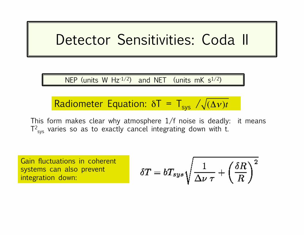
Detector Sensitivities: Coda II
NEP (units W Hz-1/2) and NET (units mK s1/2)
This form makes clear why atmosphere 1/f noise is deadly: it means T2
sys varies so as to exactly cancel integrating down with t.
(Δν )t
Gain fluctuations in coherent systems can also prevent integration down:
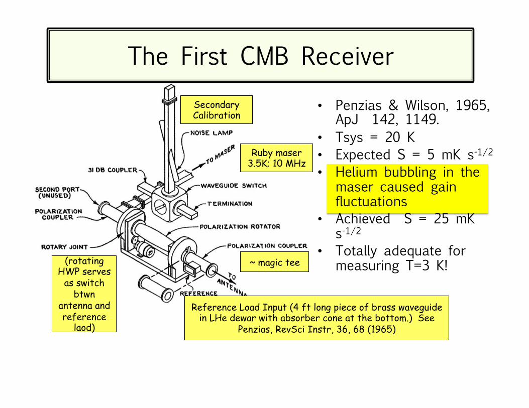
Ruby maser 3.5K; 10 MHz
(rotating HWP serves
as switch btwn
antenna and reference
laod)
~ magic tee
Reference Load Input (4 ft long piece of brass waveguide in LHe dewar with absorber cone at the bottom.) See
Penzias, RevSci Instr, 36, 68 (1965)
The First CMB Receiver Secondary Calibration
• Penzias & Wilson, 1965, ApJ 142, 1149.
• Tsys = 20 K • Expected S = 5 mK s-1/2 • Helium bubbling in the
maser caused gain fluctuations
• Achieved S = 25 mK s-1/2
• Totally adequate for measuring T=3 K!
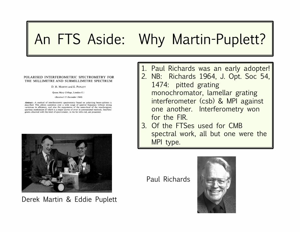
An FTS Aside: Why Martin-Puplett?
1. Paul Richards was an early adopter! 2. NB: Richards 1964, J. Opt. Soc 54,
1474: pitted grating monochromator, lamellar grating interferometer (csb) & MPI against one another. Interferometry won for the FIR.
3. Of the FTSes used for CMB spectral work, all but one were the MPI type.
Paul Richards
Derek Martin & Eddie Puplett

An FTS Aside: Why Martin-Puplett?
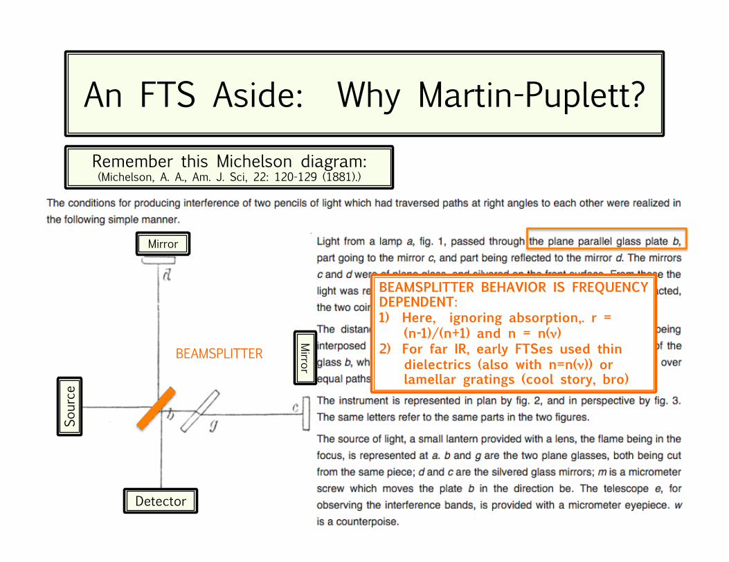
Remember this Michelson diagram: (Michelson, A. A., Am. J. Sci, 22: 120-129 (1881).)
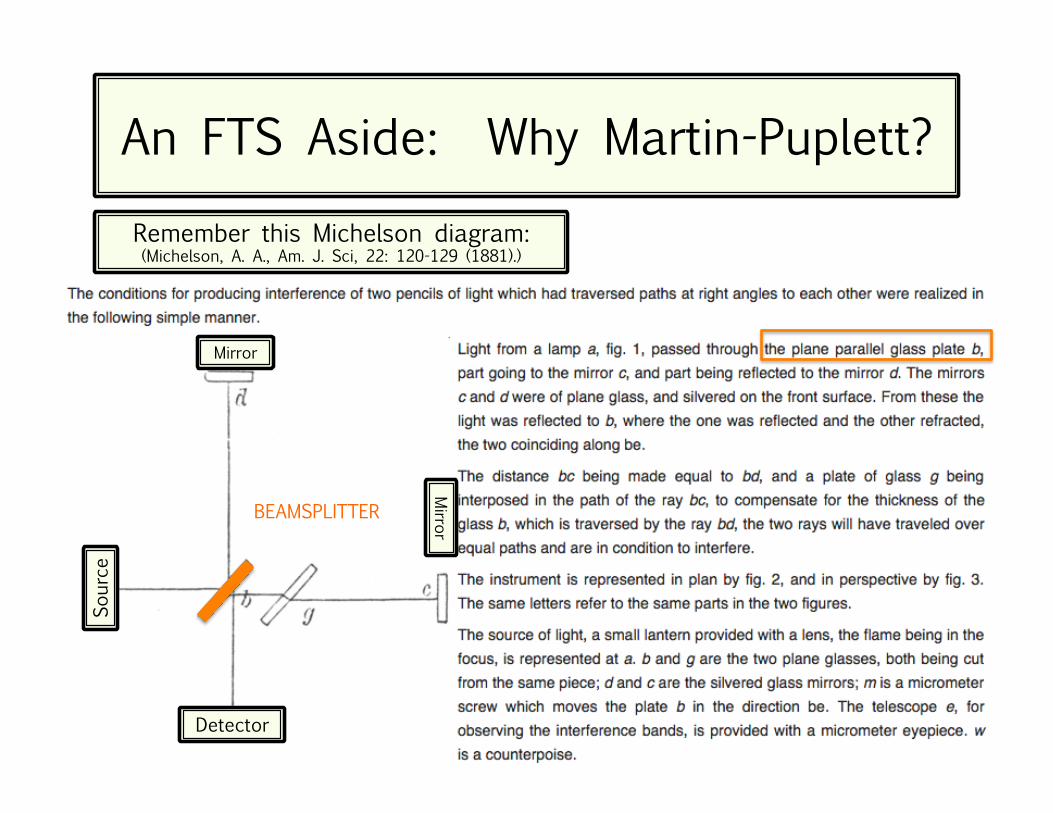
An FTS Aside: Why Martin-Puplett? So
urce
Detector
Mirror
Mirror
BEAMSPLITTER
Remember this Michelson diagram: (Michelson, A. A., Am. J. Sci, 22: 120-129 (1881).)
An FTS Aside: Why Martin-Puplett? So
urce
Detector
Mirror
Mirror
BEAMSPLITTER
Remember this Michelson diagram: (Michelson, A. A., Am. J. Sci, 22: 120-129 (1881).)
BEAMSPLITTER BEHAVIOR IS FREQUENCY DEPENDENT: 1) Here, ignoring absorption,. r =
(n-1)/(n+1) and n = n(ν) 2) For far IR, early FTSes used thin
dielectrics (also with n=n(ν)) or lamellar gratings (cool story, bro)
Pin
Pout
BS
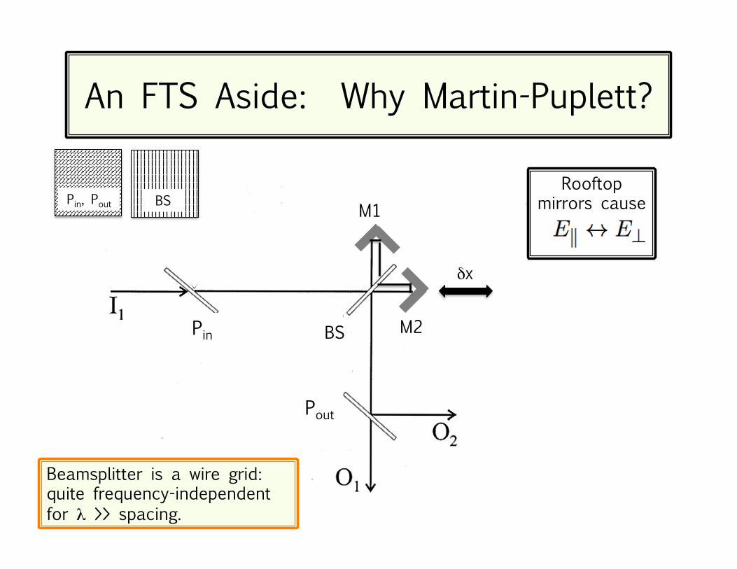
An FTS Aside: Why Martin-Puplett?
Pin, Pout BS M1
M2
δx
Rooftop mirrors cause
E ß> Ey
Beamsplitter is a wire grid: quite frequency-independent for λ >> spacing.
Pin
Pout
BS
An FTS Aside: Why Martin-Puplett?
Pin, Pout BS M1
M2
δx
Rooftop mirrors cause
E ß> Ey
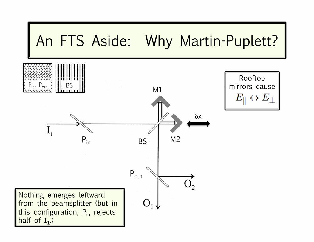
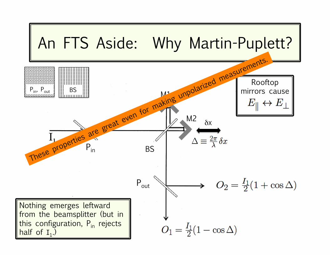
Nothing emerges leftward from the beamsplitter (but in this configuration, Pin rejects half of I1.)

An FTS Aside: Why Martin-Puplett?
Pin
Pout
BS
M1
M2 δx
Pin, Pout BS
Nothing emerges leftward from the beamsplitter (but in this configuration, Pin rejects half of I1.)
Rooftop mirrors cause
E ß> Ey
Foreshadows form of PIXIE 2-beam outputs!
An FTS Aside: Why Martin-Puplett?
Pin
Pout
BS
M1
M2 δx
Pin, Pout BS
Nothing emerges leftward from the beamsplitter (but in this configuration, Pin rejects half of I1.)
Rooftop mirrors cause
E ß> Ey
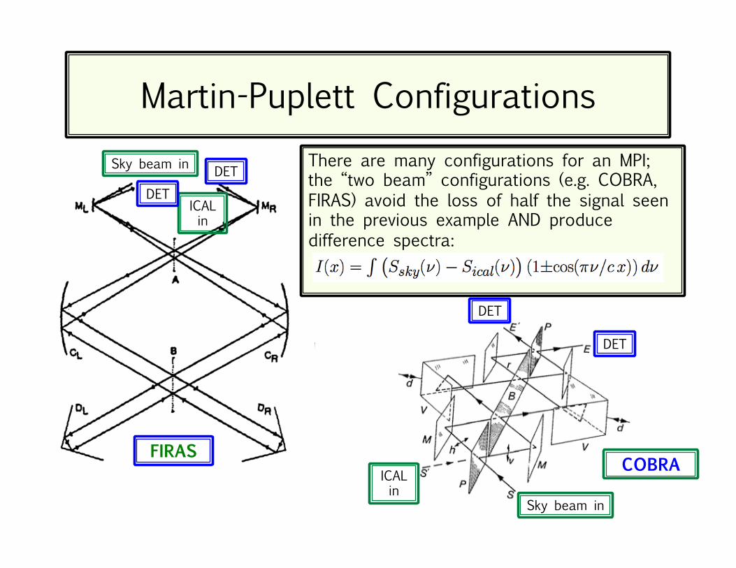
Martin-Puplett Configurations There are many configurations for an MPI; the “two beam” configurations (e.g. COBRA, FIRAS) avoid the loss of half the signal seen in the previous example AND produce difference spectra:
Sky beam in
ICAL in
DET DET
FIRAS
Sky beam in
ICAL in
DET
DET
COBRA
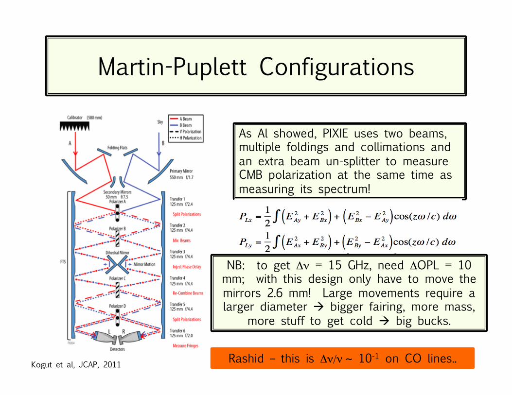
Martin-Puplett Configurations
As Al showed, PIXIE uses two beams, multiple foldings and collimations and an extra beam un-splitter to measure CMB polarization at the same time as measuring its spectrum!
Kogut et al, JCAP, 2011
NB: to get Δν = 15 GHz, need ΔOPL = 10 mm; with this design only have to move the mirrors 2.6 mm! Large movements require a larger diameter à bigger fairing, more mass,
more stuff to get cold à big bucks.
Rashid – this is Δν/ν ~ 10-1 on CO lines..
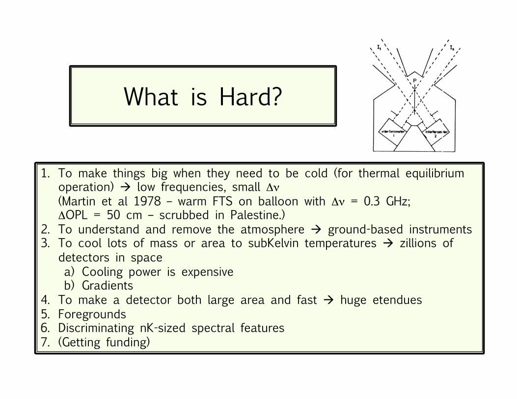
What is Hard?
1. To make things big when they need to be cold (for thermal equilibrium operation) à low frequencies, small Δν (Martin et al 1978 – warm FTS on balloon with Δν = 0.3 GHz; ΔOPL = 50 cm – scrubbed in Palestine.)
2. To understand and remove the atmosphere à ground-based instruments 3. To cool lots of mass or area to subKelvin temperatures à zillions of
detectors in space a) Cooling power is expensive b) Gradients
4. To make a detector both large area and fast à huge etendues 5. Foregrounds 6. Discriminating nK-sized spectral features 7. (Getting funding)
Hard <> Impossible!
END