Experimenting with Independent And-Parallel Prolog using Standard Prolog M. V. Hermenegi ldo herme@fi.upm.es or herme@cs.utexas.edu

M. Carro borisOfi .upm.es

Universidad Politecnica de Madrid (UPM) Facultad de Informatica 28660-Boadilla del Monte, Madrid - SPAIN

Abstract

This paper presents an approximation to the study of parallel systems using sequential tools. The Independent And-parallelism in Prolog is an example of parallel processing paradigm in the framework of logic programming, and implementations like <fc-Prolog uncover the potential performance of parallel processing. But this potential can also be explored using only sequential systems. Being the spirit of this paper to show how this can be done with a standard system, only standard Prolog will be used in the implementations included. Such implementations include tests for parallelism in And-Prolog, a correctness-checking meta-interpreter of <fc-Prolog and a simulator of parallel execution for <fc-Prolog.

1 Introduction

There are many types of parallel processors in the marketplace today, and multiprocessor systems are expected to be the norm in the very near future. However, the amount of software that can exploit the performance potential of these machines is still very small. This is due to two main reasons:

• Traditionally, to exploit fully potential multiprocessors, issues like task dependencies and even machine topology had to be considered. This is a task that can become extremely difficult and highly error-prone. Karp points out [10] that "the problem with manual parallelization is that much of the work needed is too hard for people to do. For instance, only compilers can be trusted to do the dependency analysis needed to parallelize programs on shared-memory systems."

• In addition, the programming languages that are conventionally parallelized have a complex imperative semantics which makes compiler analysis difficult and forces users to employ control mechanisms that hide the parallelism in the problem.

These two drawbacks can be somewhat avoided with the progress to systems that do not require explicit creation and mapping of processes to a given topology and with the appear­ance and success of declarative languages. Declarative languages and, in particular, logic programming languages, require far less explication of control (thus preserving much more of the parallelism in the problem). In addition, their semantics makes them comparatively

more amenable to compile-time analysis and program parallelization. In other words, such programs preserve more the intrinsic parallelism in the problem, make it easier to extract in an automatic fashion, and allow the techniques being used to be proved correct. Therefore, we will focus on parallelism in a logic programming framework. Some questions might posed:

• How good is the automatic parallelizers performance? In other words, how much par­allelism and conditions of parallelism can be automatically uncovered?

• How much do the parallelism tests cost, and how ought them be implemented?

• In real applications, how often do the parallelism conditions hold, i.e., how much real parallelism can be achieved?

The aim of this paper is to show how such questions can be explored without the needing of neither a parallel system nor very elaborated software. This paper is not intended to be a piece of theoretical work, but rather a practical one to be consulted by those who want to explore parallelism "in their garage". Our purpose is to develop code to check parallelism conditions in &-Prolog and to interpret &-Prolog, giving, as well, information about the performance of the tested programs. It is to be noted that all this work has been done in Prolog, so that it can run on any standard system.

We will proceed as follows: in Section 2 independent And-parallelism will be explained. &-Prolog system features will be presented in Section 3. In Section 4 some code related with run-time checks will be discussed; this will be continued in Section 5. The first meta-interpreter will be developed in Section 6, and in Section 7 a simulator of &-Prolog will be introduced.

2 Overview of Independent And-Parallelism

Two kinds of parallelism are being currently studied in the Prolog arena: Or- and And-parallelism; several models have been proposed to take advantage of the opportunities they offer (see, for example, [3], [13], [1], [5], [11], [18], [4], [17], [15] and their references). Or-parallelism refers to the parallelism between clauses of a predicate, while And-parallelism refers to parallelism between goals in a clause body. But it may not be advantageous to run all goals in parallel: conditions of data dependency and efficiencyrestrict the set of parallelizable goals. IAP model selects particular goals based on efficiency considerations: only goals such that the result of one does not depend of the results of the others can be run in parallel. Such goals are called independent, and independence is a sufficient condition for parallel execution.

The theoretical research on And-parallel Prolog provides the following results [9, 8]:

• (Correctness and completeness) If only independent goals are executed in parallel the solutions obtained are the same as those produced by standard sequential execution.1

• In the absence of failure, parallel execution does not generate additional work (with respect to sequential execution) while actual execution time is reduced.

• In the case of failure the parallel execution is guaranteed to be no slower than the sequential execution.

lrThe finite failure set can be larger, this being understood as a desirable characteristic.

Although independence can be checked at run-time, it is more efficient to check it at compile time. Conditions of independence are given in [8, 9], and are usually expressed in terms of groundness and independence of variables. Groundness and independence refer to the existence of variables in a term and to the sharing of variables between two (or more) terms, respectively. Let T be a term and var(T) the set of all free variables in T. Then groundness and independence are defined as follows:

Definition 1 (Groundness) A term T is ground if the set of all variables in T is empty: ground{T) = var{T) = 0.

Definition 2 (Strict independence) Two terms T and U are said to be strictly indepen­dent if they do not share variables: indep(T,U) = var{T) f| var{U) = 0.

In absence of side effects, ground goals can run in parallel with any other goal, and strictly independent goals can also run in parallel.

3 Overview of the &-Prolog System

The &-Prolog system comprises a parallelizing compiler aimed at uncovering IAP and an execution model/run-time system aimed at exploiting such parallelism. The run-time system is based on the Parallel WAM (PWAM) model, an extension of RAP-WAM [5, 6], itself an extension of the Warren Abstract Machine (WAM) [16]. Figure 1 shows the conceptual structure of the &-Prolog system. Although the compiler components are depicted in this figure as separate modules, they have been integrated into the Prolog run-time environment in the usual way. It is a complete Prolog implementation, offering full compatibility with the DECsystem-20/Quintus Prolog ("Edinburgh") standard, plus supporting the &-Prolog language extensions, which will be described in section 3.1.

3.1 The &-Prolog Language

We define a new language called &-Prolog as a vehicle for expressing and implementing strict and non-strict IAP. &-Prolog is essentially Prolog, with the addition of the parallel conjunc­tion operator "&" (used in place of "," -comma- when goals are to be executed concurrently)2

and a set of parallelism-related builtins, which includes several types of groundness and in­dependence checks, and synchronization primitives. Combining these primitives with the normal Prolog constructs, such as "->" (if-then-else), users can conditionally trigger paral­lel execution of goals. For syntactic convenience, an additional construct is also provided: the Conditional Graph Expression (CGE). A CGE has the general form (i_cond => goal\ & goal2 & . . . & goaljsj) where the goak are either normal Prolog goals or other CGEs and Lcond is a condition which, if satisfied, guarantees the mutual independence of the goaks. The CGE can be viewed simply as syntactic sugar for the Prolog conditional construct:

( i-cond -> goal\ & goali & . . . & goalj^ ; goal\ , goali , • • • , goaljy )

2 The backward operational semantics (backtracking) of the "&" construct is conceptually equivalent to standard backtracking except that dependency information is used to economically perform a limited form of intelligent backtracking. See [7, 5] for details.

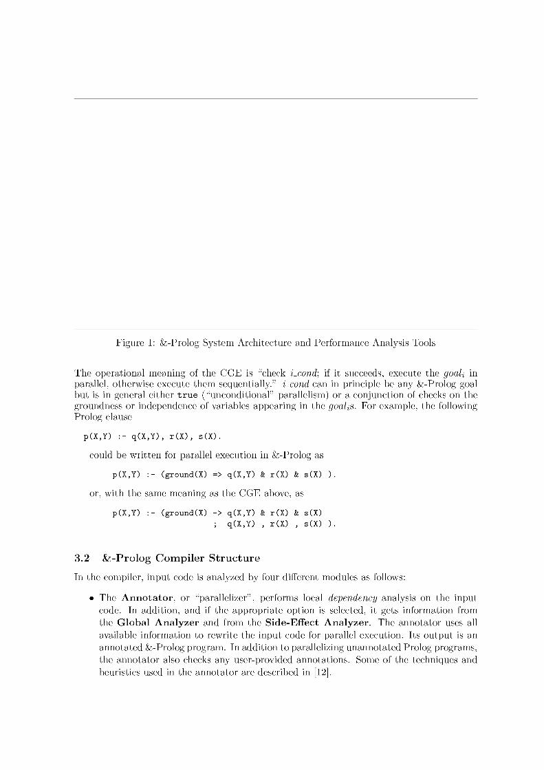
Figure 1: &-Prolog System Architecture and Performance Analysis Tools

The operational meaning of the CGE is "check Lcond; if it succeeds, execute the goak in parallel, otherwise execute them sequentially." Lcond can in principle be any &-Prolog goal but is in general either t rue ("unconditional" parallelism) or a conjunction of checks on the groundness or independence of variables appearing in the goaks. For example, the following Prolog clause

p(X,Y) : - q (X ,Y) , r ( X ) , s ( X ) .

could be written for parallel execution in &-Prolog as

p(X,Y) : - (ground(X) => q(X,Y) & r (X) & s(X) ) .

or, with the same meaning as the CGE above, as

p(X,Y) : - (ground(X) -> q(X,Y) & r (X) & s(X) ; q(X,Y) , r (X) , s(X) ) .

3.2 &-Prolog Compiler Structure

In the compiler, input code is analyzed by four different modules as follows:

• The Annota tor , or "parallelizer", performs local dependency analysis on the input code. In addition, and if the appropriate option is selected, it gets information from the Global Analyzer and from the Side-Effect Analyzer. The annotator uses all available information to rewrite the input code for parallel execution. Its output is an annotated &-Prolog program. In addition to parallelizing unannotated Prolog programs, the annotator also checks any user-provided annotations. Some of the techniques and heuristics used in the annotator are described in [12].

• The global analyzer interprets the given program over an abstract domain (specifically designed to precisely highlight dependence information) and infers information about the possible run-time substitutions at all points of the program.

• The side-effect analyzer annotates each non-builtin predicate and clause of the given program as pure, or as containing or calling a side-effect.

• The low-level PWAM Compiler (an extension of the SICStus0.5 WAM compiler [2]) produces PWAM code from a given &-Prolog program.

4 Implementing Groundness and Independence Checks

Groundness and independence checks are essential for a full exploitation of parallelism; in most cases the compiler cannot extract all the information needed to ensure the correctness of parallel execution, and run-time tests turn out to be necessary to uncover the possible parallelism. Therefore, a given program can show different degrees of parallelism according to the toplevel query; this characteristic is not easily found in imperative languages. These tests take some time to be completed, but it is expected that that the gain of parallel execution compensate largely for it. They can be implemented as natives, but it will be shown how they can be easily implemented in Prolog. Both versions (native and coded in Prolog) can be found in the &-Prolog system builtins.

Although the definition of groundness and independence is very clear, practical checks can be full or conservative. "Full checks" means that no wrong decision will ever be made; on the other hand, conservative checks sometimes do not give us the correct answer, but the wrong answer given is always the safest: for example, a ground term can be decided to be non ground, but the opposite can never occur. We will concentrate now on full checks; conservative checks will be discussed in Section 5.

4.1 Full Groundness Check

The definition of groundness suggests a naive implementation: the term to be inspected is traversed and its variables collected in a set. Then the emptyness of the set is checked. If the set is empty the term is ground.

naive_ground(T):-se t_of .va r i ab les (T , S) , empty_set(S).

This is a correct method, but traversing the whole term is always necessary. An easy improvement stems from the following consideration: a term is non ground if it contains at least one variable. So all we have to do is to traverse the term and stop when the first variable is found, with the result of non groundness. If no variable is found, the term is ground.

Here follows the groundness check as it appears in the &-Prolog system3 builtins. Free variables are not ground; terms are traversed from the last component to the first, and each component is also tested for groundness. This also covers the case of an atom, which is simply a term of arity 0.

3As we said before, in addition to this code the &-Prolog system includes code for testing groundness and independence written in C.

ground(Term):-nonvar(Term), functor(Term,_,N), ground(N,Term).

ground(N,Term):-N > 0, arg(N,Term,Arg), ground(Arg), Nl i s N- l , ground(Nl,Term).

ground(0,_) .

It is clear that this algorithm is better than the naive one when the term is non ground. But it should be noted that in the future sofisticated analysis and better compiler technology could be able to give better conditions of parallelism. So it is likely that goals annotated as parallelizable be almost always run in parallel (perhaps using low-level synchronization), and the conditions of parallelism would rarely fail. The point in this is that the above implementation of ground/1 takes its advantage over the naive-ground/'1 implementation when the term is non ground, i.e., when the test fails. If the tests are expected to fail very few times, the real performance of the naive_ground/l will be very close to ground/1, being the first clearer and closer to the logic definition.

4.2 Full Independence Check

Again, the naive independence test is based on the definition. It consists of traversing the two terms collecting their sets of variables and checking its intersection:

naive_indep(Tl, T2) : -se t_of_var iables(Tl , S I ) , se t_of .va r iab les (T2 , S2), i n t e r s e c t i o n ( S l , S2, I ) , empty_set(I) .

intersection/1 is supposed to be able to make the intersection of two sets of variables, which implies checking their logic identity. The cost of this implementation is very high: two terms have to be traversed and one intersection has to be done. Recalling the definition of independence, it is easy to see that the groundness of one term implies the independence of the two terms; so we can assure independence as soon as on term is found to be ground.

less_naive_indep(Tl , T2) : - \+ naive_dep2(Tl, T2). naive_dep2(Tl, T2) : -

se t_of_var iables(Tl , S I ) , \+ empty_set(SI) , se t_of .va r iab les (T2 , S2), \+ empty_set(S2), i n t e r s e c t i o n ( S l , S2, I ) , \+ empty_set(I) .

Should the terms be often ground, this test is, on the average, faster than naiveJndep/2, but slightly slower otherwise.

A better algorithm for checking independence is as follows: the first term is traversed and each variable found is marked, i.e., unified with a given value. Then the other term is traversed; if a mark is found, we know that at least one variable was shared. The use of cut and fail automatically resets to unbound the marked variables. One improvement added to this algorithm is that if no variables are found when the first term is traversed, there is no need of traversing the second one.

indep(A,B) :-

mark(A,Ground), °/0 Ground is var if A ground

nonvar(Ground), °/0 If 1st argument was ground, no need to proceed

marked(B), !, fail.

indep(_,_).

mark('$Space$Oddity$', no ) :- !. °/0 Found a variable, mark it

mark( Atom , _ ) :- atomic(Atom),!.

mark(Complex , GR) :- mark(Complex,1,GR).

mark(Args,Mth,GR) :-

arg(Mth,Args,ThisArg),!,

mark(ThisArg,GR),

Nth is Mth+1,

mark(Args,Nth,GR). mark(_,_,_).

marked( Term ) :-

functor(Term,F,A),

( A > 0, !, marked(Term,1)

; F = '$Space$0ddity$' ).

marked(Args,Mth) :-

arg(Mth,Args,ThisArg),!, ( marked(ThisArg) ; Nth is Mth+1,

marked(Args,Nth)).

In comparison with the two first implementations, this one traverses the two terms only in the worst case, which is a significant improvement.

5 Other Groundness and Independence Checks

In this section other approaches to groundness and independence checks are discussed. In some cases they are only variations or suggestions of improvements over former algorithms, but in other cases they represent a completely new approach. First of all it will be shown how to count the number of variables in a term, because it will be used in some examples.

5.1 Counting Variables

Most Prologs have an efficiently implemented builtin predicate, numbervars/2, which is used to find out and number the number of different variables in a term. This predicate can be used to implement easily groundness and independence checks. We will show here how it can be implemented in Prolog.

We will use a technique similar to that of Section 4.2: each variable will be marked with a different number, and the number of marks used will give us the number of variables. This will bind all free variables; to undo the bindings the technique is to record the number of variables found and then fail. When the second alternative is tried, variable bounds are reset and the recorded number can be recovered and erased.

°/0 numbervar s (T , N) i f t h e number of v a r s of t h e term T i s N.

numbervars(Term, _ ) : -

numbervars(Term, 0, Number),

recorda('$NvArS', Number, _ ) , fail. °/0 We record and fail numbervars(_, Number):-

recorded('$NvArS', Number, Ref), °/0 Collect the recorded number erase(Ref).

°/0 Count the number of different vars, using accumulation parameter

numbervars(X,N,Nl)

numbervars(A,N,N)

numbervars(F,N,Nl)

var(X), !, Nl is N+l, X='$VAR'(N).

atomic(A), !.

numbervars(0,F,N,Nl).

numbervars(I,F,N,Nl) :-II is 1+1, arg(Il,F,X),

numbervars(X,N,NO), !,

numbervars(II,F,NO,Nl). numbervars(_,_,N,N).

Note that numbervars/2 always traverses the whole term.

5.2 Groundness Checks

The groundness check already seen explicitly traverses the term to be inspected; this performs a full check. The number of variables of the term can also be used: a term is ground if it contains no variables at all. So it can be written:

nvground (Te rm) : - numberva r s (Te rm,0 ) .

This has a major drawback: the whole term has to be always traversed by numbervars/2, while ground/1 can decide non groundness when the first variable is found. Now, let's sup­pose we have a huge ground term. Both ground/1 and nvground/1 will have to traverse it completely. This poses a problem: in case of very large terms, it can be more expensive decid­ing about the groundness than giving up the search and running the goals sequentially. This can be partially controlled with a new version of the groundness test in which the maximum depth search is given. If this level is reached and no variable has been found yet, the term is conservatively supposed non ground. It should be noted that the search done is depth-first, so the meaning of the failure of the predicate is not the absence of variables in the N first levels of the term tree, but the existence of a path of length N from the tree root which does not contain variables. The code is as follows:

l g r o u n d ( T e r m , D e p t h ) : -Depth>0, nonva r (Te rm) , f u n c t o r ( T e r m , _ , N ) , NDepth i s D e p t h - 1 , lg round(N,Term,NDepth) .

l g r o u n d ( N , T e r m , D e p t h ) : -N>0, a r g ( N , T e r m , A r g ) , l g r o u n d ( A r g , D e p t h ) , Nl i s N - l ,

l g r o u n d ( N l , T e r m , D e p t h ) . l g r o u n d ( 0 , _ , _ ) .

Last, the minimum groundness check and the simpler one; it is highly conservative but also very efficient, because it relies completely on a native predicate. It only checks if the term is an atom. A wrong answer will be given only if the term is a non ground structure, and in this case it is supposed to be ground, which is safe.

mground(Term) : - a tomic (Te rm) .

5.3 Independence Checks

We will proceed here as we did in the previous section. First of all we will show how number-vars/2 can be used to make an independence check of two terms. The underlying idea is very simple: if the terms A and B are independent, then the number of variables in foo(A, B) is the sum of the number of variables in A plus the number of variables in B, because no variables are shared by A and B.

nvindep(A, B ) : -numbervars(A, Na) , numbervars (B, Nb) , numbervars ( foo(A, B ) , Nfoo) , Nfoo i s Na + Nb.

Again, these terms have to be completely traversed. The technique used in less-naiveJndep/2 can be applied here: if a term contains no variables, the two terms are independent.

nvindep2(A, B ) : - \+ nvdep(A, B ) . nvdep(A, B ) : -

numbervars(A, 0 , Na ) , Na \== 0 , numbervars (B, 0 , Nb) , Nb \== 0 , numbervars ( foo(A, B ) , 0 , Nfoo) , Nfoo \== Na + Nb.

It should be pointed out that we are using here numbervars/3 instead of numbervars/2, so that there is a gain of efficiency (no recording is needed). The terms A and B remain untouched after the call to nvindep/2 due to the negation.

The problem of big terms also arises when testing for independence. The solution is the same: a depth limit can be given in the initial call. If the search tries to go beyond this limit, it will fail.

°/0 T e s t s i ndependence , w i th a l i m i t e d s e a r c h d e p t h

l i n d e p ( T A , T B , D e p t h ) : - \+ ldep(TA,TB,Dep th ) .

ldep(TA,TB,Depth):-

lmark(TA,Depth, Ground), °/0 if lmark succeeds, it all depends on lmarked.

lmarked(TB,Depth).

ldep(_,_,_). °/0 i.e. if lmark fails, conclude it is dependent.

°/0 Marks all variables in Term with a magic value or fails if deeper than Depth.

lmark C$$Mark' , _ ) : - ! .

lmark(A,_) :- atomic(A), !.

lmark(F,Depth) :- ND is Depth-1, ND > 0, lmark(l,F,ND).

lmark(I,F,D) :-

arg(I,F,ArgI), !, lmark(ArgI,D), NI is 1+1, lmark(NI,F,D).

lmark(_,_,_,_).

7o Succeeds if F contains a magic value or is larger than Depth.

lmarked(F,D) :-

functor(F,_,A), ( A=0,

F == '$$Mark' ; ND is D-l,

( ND < 0 ; lmarked(l,F,D))).

lmarked(I,F,D) :-

arg(I,F,Arg), !, ( lmarked(Arg,D) ; II is 1+1,

lmarked(Il,F,D)).

To finish with this section we will look at the minimum independence check: two terms A and B are independent if they are variables which do not share. In fact this is DeGroot's algorithm, and is a very fast test, because in a WAM implementation of Prolog it is reduced to the dereferencing of the variables and the comparison of two addresses.

mindep(A, B ) : - v a r ( A ) , v a r ( B ) , A \== B.

6 Meta-Interpreting &-Prolog

In most cases it is necessary to simulate a system, being the reasons very different: the system does not exist yet or does not work correctly or is not available at a given time and/or place. Anyway, a simulation is always interesting, because it is usually cheaper to develop and experiment with, and easier to modify than the real system.

In this section we will simulate &-Prolog execution through the development of a small meta-interpreter completely written in Prolog. The possibility of running in standard Pro­log systems true &-Prolog programs annotated with CGEs is, therefore, offered, as well as the opportunity of checking the correctness of annotated &-Prolog programs and automatic parallelization tools.

6.1 A Minimum Meta-interpreter

A minimum meta-interpreter for &-Prolog has to deal with the two new operators intro­duced: "&" and "=>". "&" will be given the same behavior as ",", and "=>" will ignore independence and groundness tests. If the following code is loaded on to a sequential Prolog system it will be capable of running &-Prolog programs, but no checking for groundness or independence will be done.

: - o p U O l O . x f y , [ ( & ) ] ) . : - o p ( 1 0 2 0 , x f x , [ ( = > ) ] ) .

_ => B : - c a l l ( B ) .

A & B : - c a l l ( A ) , c a l l ( B ) .

6.2 A Correctness-Checking Meta-Interpreter

As we said before, run-time checks are necessary to ensure a safe parallel execution. Even more, they are essential to simulate the behavior of &-Prolog, because the success or failure of checks drives the execution through parallelism or sequentiality. Our meta-interpreter will be improved to take into account the tests at the left of the "=>" operator and simulate or not parallelism according to the results of these tests. They can be arbitrary &-Prolog goals, but the most interesting ones are those related to groundness and independence. The ones we implemented in Section 4 and Section 5 can be freely used. It is also interesting to know how many CGEs have been satisfied and how many goals have been run in parallel, because this number can be used as a raw indication of the performance and correctness of the CGE tests.

The improvement over the former version is that the A = > B construction behaves as follows: if A fails, the goals in B are sequentially executed and a CGE failure is annotated. Otherwise, a CGE success is annotated and independence checks are made on the goals in B at run time. If these checks succeed, parallel execution of goals is simulated. If not, a warning is reported, but parallelism is also simulated. Simulating parallelism merely consists of running goals sequentially and annotating the number of goals executed. The reason for doing independence tests after succeeding the in CGE conditions is that it is possible that way to detect errors in the generation of the conditions.

This meta-interpreter does not allow the simple construction A & B; it must always be done through a CGE: (true = > A & B). To use this code p-cgeJnfo/0 has to be called between executions; collected statistics will be shown and reset. Statistics are automatically initialized when the code is first loaded.

: - o p U O l O . x f y , [ ( & ) ] ) . p a r _ c a l l ( ( A & B & O ) : - ! ,

r e c o r d _ i n c ( ' $ p a r g o a l s ' ) , c a l l ( A ) , p a r _ c a l l ( ( B & O ) .

p a r _ c a l l ( ( A & B)) : -record_inc('$pargoals'), call(A),

record_inc('$pargoals'), call(B).

°/0 If the goal is to be sequentially run, no statistics need to be updated

seq_call((A & B & O ) :- ! ,

call (A), seq_call((B & O ) .

seq_call((A & B)) :-

call(A), call(B).

°/0 For C => B: first pass conditions, then check goals for independence.

:- op(1020,xfx,[(=>)]).

C => B :-

call(C), !,

record_inc('$cge_successes'),

check_goals_or_complain(B), par_call(B).

C => B :-

record_inc('$cge_failures'),

seq_call(B).

check_goals_or_complain(B)

check_goals_or_complain(B)

write('*** Warning

write(B), nl.

- check_goals(B), !.

these parallel goals are not independent!'), nl,

°/0 Check each goal against the following ones

check_goals((A & Rest)):-

Rest = (B & NewRest), !,

check_flat_goals((A & Rest)),

check_goals((B & NewRest)). check_goals((A & B)):- indep([[A,B]]).

check_flat_goals((A & Rest)):-

Rest = (B & NewRest), !,

indep([[A,B]]), check_flat_goals((A & NewRest)).

check_flat_goals((A & B)):- indep([[A,B]]).

record_init(X):-

recorded(X,_,Ref), !, erase(Ref),

recorda(X,0,_). record_init(X):- recorda(X,0,_).

record_inc(X):-

recorded(X,Old,Ref), erase(Ref), New is Old +1, recorda(X,New,_).

p_cge_info:-recorded('$cge_successes',S,_),

recorded('$cge_failures',F,_),

recorded('$pargoals',P,_),

write(S), write(' CGEs succeeded, ' ) , nl,

write(F), write(' CGEs failed.'), nl, write(P), write(' Goals executed in parallel.'), nl,

record_init('$cge_successes'),

record_init('$pargoals'),

record_init('$cge_failures').

init :- record_initC$cge_successes'),

record_init('$pargoals'),

record_init('$cge_failures'),

write('[*** CGE counters initialized.]'), nl,

write('[*** Please remember to call p_cge_info/0 between runs.]'), nl.

7 Computing Performance of &-Prolog

The statistics collected by the meta-interpreter developed in Section 6.2 concern directly the correctness and performance of CGE tests. However, although a crude measure of parallel goals is given, no information about the performance gain attained through parallelism is ob­tained. We will show how to collect more significant statistics about the potential performance gained by &-Prolog programs. There are some characteristics that can be of interest:

• Execution time is the most cited datum about a system performance. But we are using standard Prolog throughout this report, so it is supposed that a parallel computer with &-Prolog is not available and it is not possible to measure the real execution time.

• As an approximation, we could count the number of unifications during an execution using a meta-interpreter written in Prolog. This has been done and results reported by Shen [14]. The resulting code is rather large. The aim here is to provide a minimum performance evaluation system.

• A quite simple but significant statistic could be the number of heads traversed during an execution; we will focus on it. This assumes that every head has the same computational cost, but later we will see how to achieve a better control over this point.

From now on, we will refer to the number of heads traversed as time, emphasizing it is a measure of the time spent in an execution. In section 6.2 we developed a metainterpreter. In this section we use the alternative of transforming the programto achieve satisfactory results.

7.1 First Approach

Suppose we have a Prolog program and we want to count the number of heads traversed during its execution. An easy technique to do this is to transform the original program into another one which counts the number of heads traversed. One way to do this is by adding two extra parameters to each predicate:

p(X, Y):- q(X, Y), r(X). p(a).

is transformed into

p(X, Y, HIn, H O u t ) : - q(X, Y, HIn, H2) , r ( X , H2, H3) , HOut i s H3 + 1. p ( a , HIn, H O u t ) : - HOut i s HIn + 1.

The heads traversed are counted using an input parameter and an output parameter. In a goal conjunction the output parameter of each goal is the input parameter of the next one. The head input parameter is the first goal input parameter, and the last goal output parameter plus one is the head output parameter.

In fact this will count the number of heads traversed, but only those traversed in the path from the toplevel goal to the solution, i.e., the time spent in alternatives tried but failed is

not computed. That is not what we want since the time wasted on unsuccessful search is always time to be taken into account.4

7.2 Dealing with Failure

Taking into account the failing paths would lead us to a very complicated meta-interpreter, which would have to deal explicitly with the backtracking and the cut (!). It Is much easier to transform the original program, automatically or by hand, to make it snoop itself through side effects. Side effects are necessary because of the unbinding done on backtracking; they are the only way in which saved results can be reconsulted after backtracking has been done.

We will introduce directly the basic idea of our snooper. Suppose we have a predicate p/1 defined as

p ( Y ) : - q(X, Y ) , r ( Y ) . p ( a ) .

This predicate is given a reference by its father (the predicate which calls it). Such reference acts like an unique bank account number to which the accounting of the work made by p/1 is to be addressed. This reference is preserved through execution and backtracking, thus reflecting the amount of work done by p/1. Of course, q/2 and r/1 must receive their own references. The point is that the work done by them is separately accounted and added to that of p/1 through its reference. Let's see how the transformed predicate looks like:

p(R, Y) : - °/0 R references the time spent by p/2 inc_time(R), seq_time(q(_, X, Y), R), seq_time(r(_, Y), R).

p(R, a ) : - inc_time(R).

First of all, every predicate must increment its arity by one to make room for the ref­erence; the variable R is the reference passed by the caller, and must be different from all other variables in the head and be placed in first place. This does not affect the number of successfully matched heads. incJ.ime/1 deals with the increment of time: the time charged to the reference passed as its argument is incremented by one. Each goal in the clause must be passed as an argument to seqJ.ime/2, which executes it. R must also be passed to seqJ.ime/2 so that the reference to charge in the time spent by q/3 and r/2 be known by it. The void argument in q/3 and r/2 is the one needed for the reference, but it is not relevant at this level. Seeking for a new reference and properly accounting the time spent is seq-time/2 business.

The toplevel goal must be called with the predicate explore/2, which acts as an interface, initializing the global time and providing the first reference, explore/1 is to be called as explore(Goal, Time), where Goal is the goal to be solved; successive solutions (if there is any) are given on backtracking. Time is the time taken to find the actual solution; after the last solution is found a message is issued, notifying the time past from the last solution to the end of the search. If the search is stopped before it ends, garbage will remain in the database, and incorrect results would be obtained later. To avoid this the predicate clean/0 is provided. It can be called at any time, but it must be always called after an incomplete search.

Supporting parallel calls is also very easy. Let's suppose the following predicate

p ( Y ) : - q(X, Y) & r ( Y ) , s ( X ) . p ( a ) .

4Remember one golden rule: failing search paths should be pruned as soon as possible.

and that q/2 and r/1 meet conditions to run in parallel. The transformation to be done is similar, but we have to use a different driver for the parallel predicates:

p(R, Y ) : -i n c _ t i m e ( R ) , p a r _ t i m e ( [ q ( _ , X, Y ) , r ( _ , Y ) ] , R ) , s e q _ t i m e ( s ( _ , X) , R ) .

p(R, a ) : - i n c _ t i m e ( R ) .

Again, the parallel goals must be enclosed within the parallel driver, in this list, and the reference passed from driver to driver. The parallelism is supposed to be ideal: the number of processors is unbound, no time is spent on scheduling, nor in creating parallel agents, etc. The model described in Section 3.1 is exactly followed with respect to the account of times.

It Is to be noted that the predicates must be rewritten (if needed) so that the goals be simple, i.e., something like

p(X):- q(X) & (r(Y),s(X, Y)).

must be firstly transformed into

p ( X ) : - q(X) & aux(X, Y) . aux(X, Y ) : - r ( Y ) , s (X, Y) .

Also, the standard CGE notation is not supported. It means that the A = > B & C construction must be rewritten as A -> B & C; B, C, and then transformed to include the sequential and parallel drivers. An example will be given below.

The general transformation is as follows:

• Each predicate to be snooped must be rewritten so that a new parameter appears in the first position of the head. This parameter represents a reference to the time spent by this predicate.

• Snooped predicates must be called through the drivers seq-time/2 and par-time/2. The reference of the father is the second parameter of the drivers.

• An increment of time must be placed in every snooped predicate, usually after the head.

Actually, the rules above are only a general indication. They do not have to be strictly obeyed, and interesting results can be obtained. We will focus on this point in the next section.

7.3 Tricky Account ings

It is the rewriter responsability to decide what cost to assign to each predicate: for example, in predicates with very complicated heads the cost of unifying them can be higher than the unit. The way to do it is using the provided predicate add-time/2 as follows:

p(R, f (X , [ a , b , k ( 0 , 1 ) | _ ] , g ( 0 , X, - 1 ) ) ) : - add_t ime(R, 2 ) .

R is the reference passed by the father. The head is quite complicated, and add-time(R, 2) keeps track of this by adding a penalty of two units of time. On the other hand, it is possible not to add time at all in a clause, thus making it inexpensive.

Builtin predicates also spend time, but in general it is not a good idea to modify them (being it impossible in case of native predicates). To take this into account, a given amount of time can simply be added after success of such goals. Let's have a look at this example:

one_zero(X, Y ) : - number(X), number(Y), X + Y =\= 0 , X * Y =:= 0.

In addition to the initial call, there are some tests which take some time. A possible way to take this into account is

one_zero(R, X, Y ) : -i n c _ t i m e ( R ) , number(X), number(Y), i n c _ t i m e ( R ) , X + Y =\= 0 , X * Y =:= 0 , add_t ime(R, 2 ) .

In fact, this is a step towards a higher time control; for example, unification control time can be as fine as desired by hand-coding the head in the body using a WAM-like Prolog code. Referring to the example with the complicated unification, it could be rewritten as:

p(R, A l ) : -i n c _ t i m e ( R ) , Al = f (X, X3, X4), i n c _ t i m e ( R ) , X4 = g ( 0 , X, - 1 ) , i n c _ t i m e ( R ) , X5 = [a , b , X 6 | _ ] , i n c _ t i m e ( R ) , X6 = k ( 0 , 1 ) , i n c _ t i m e ( R ) .

In this way, parameter passing is decomposed in a step-by-step fashion, each step being considered separately. Unfortunately indexing has been impacted by the use of call/1, which means that in this case the accounting cannot be very accurate. To conclude, not every user predicate has to be transformed, but only those which are selected to contribute to their father execution time.

We will show now a full example of how to transform a well known benchmark: hanoi with granularity control. The initial code is as follows:

a p p e n d ( [ ] , L , L ) . a p p e n d ( [ H | L ] , L 1 , [ H I T ] ) : - a p p e n d ( L , L I , T ) .

hanoi(l, _, A,_,C,[mv(A,C)]). hanoi(N, G, A,B,C,M) :-

N > 1, Nl is N - 1,

(grain(N, G) => hanoi(Nl,G,A,C,B,M1) & hanoi(Nl,G,B,A,C,M2)),

append(Ml,[mv(A,C)|M2],M).

grain(N, G):- N < G.

main(N, G):- hanoi(_, N, G, a, b, c, _ ) .

In the transformed code we will consider that arithmetical operations spend two time units, and that the grain control is costless (this is only an example, to cover all possibilities). If grain control is costless, there is no real need to transform the predicate grain/2, and can be left as is. The CGE has to be rewritten, and the final code is:

append(R, [ ] , L , L ) : - i n c _ t i m e ( R ) . append(R, [ H | L ] , L 1 , [H|T]) : - i n c _ t i m e ( R ) ,

s e q _ t i m e ( a p p e n d ( _ , L , L 1 , T ) , R ) .

hanoi(R, 1, _, A,_,C,[mv(A,C)]):- inc_time(R). hanoi(R, N, G, A,B,C,M) :- inc_time(R),

N > 1, Nl is N - 1,

add_time(R, 2), °/0 Penalty for arithmetical operations

( g r a i n ( N , G) -> % Gra in c o n t r o l ^ inexpensive. p a r _ t i m e ( [ h a n o i ( _ , N l , G , A , C , B , M l ) , h a n o i ( _ , N l , G , B , A , C , M 2 ) ] , R)

; s e q _ t i m e ( h a n o i ( _ , N l , G, A, C, B, Ml ) , R ) , s e q _ t i m e ( h a n o i ( _ , N l , G, B, A, C, M2), R)

) ,

seq_time(append(_, Ml,[mv(A,C)|M2],M), R) .

grain(N, G):- N < G.

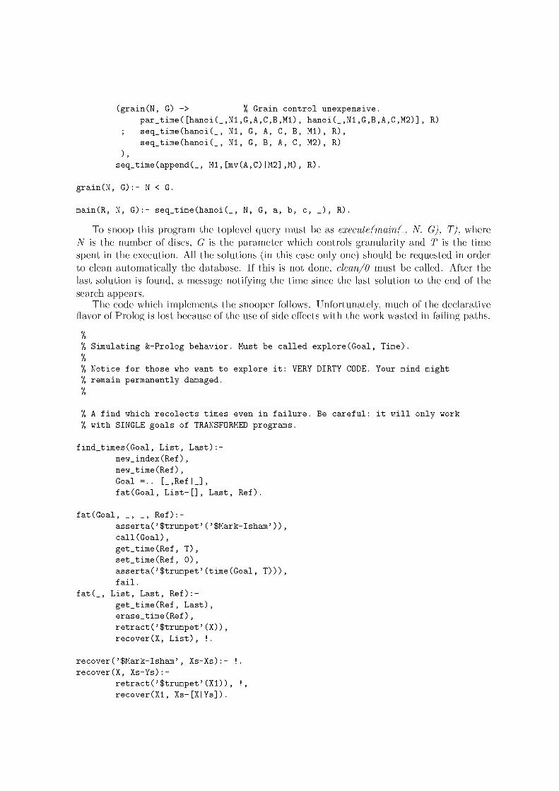
main(R, N, G):- seq_time(hanoi(_, N, G, a, b, c, _ ) , R).

To snoop this program the toplevel query must be as execute (main (-, N, G), T), where N is the number of discs, G is the parameter which controls granularity and T is the time spent in the execution. All the solutions (in this case only one) should be requested in order to clean automatically the database. If this is not done, clean/0 must be called. After the last solution is found, a message notifying the time since the last solution to the end of the search appears.

The code which implements the snooper follows. Unfortunately, much of the declarative flavor of Prolog is lost because of the use of side effects with the work wasted in failing paths.

7. °/0 Simulating &-Prolog behavior. Must be called explore (Goal, Time).

7. °/0 Notice for those who want to explore it: VERY DIRTY CODE. Your mind might 7o remain permanently damaged. 7.

°/0 A find which recolects times even in failure. Be careful: it will only work

% with SINGLE goals of TRANSFORMED programs.

find_times(Goal, List, Last):-

new_index(Ref),

new_time(Ref),

Goal =.. [_,Ref|_],

fat(Goal, List-[], Last, Ref).

fat(Goal, _, _, Ref):-

asserta('$trumpet'('$Mark-Isham')), call(Goal),

get_time(Ref, T), set_time(Ref, 0),

asserta('$trumpet'(time(Goal, T))),

fail. fat(_, List, Last, Ref):-

get_time(Ref, Last), erase_time(Ref),

retract('$trumpet'(X)),

recover(X, List), !.

recover('$Mark-Isham', Xs-Xs):- !. recover(X, Xs-Ys):-

retract('$trumpet'(XI)), !,

recover(Xl, Xs-[X|Ys]).

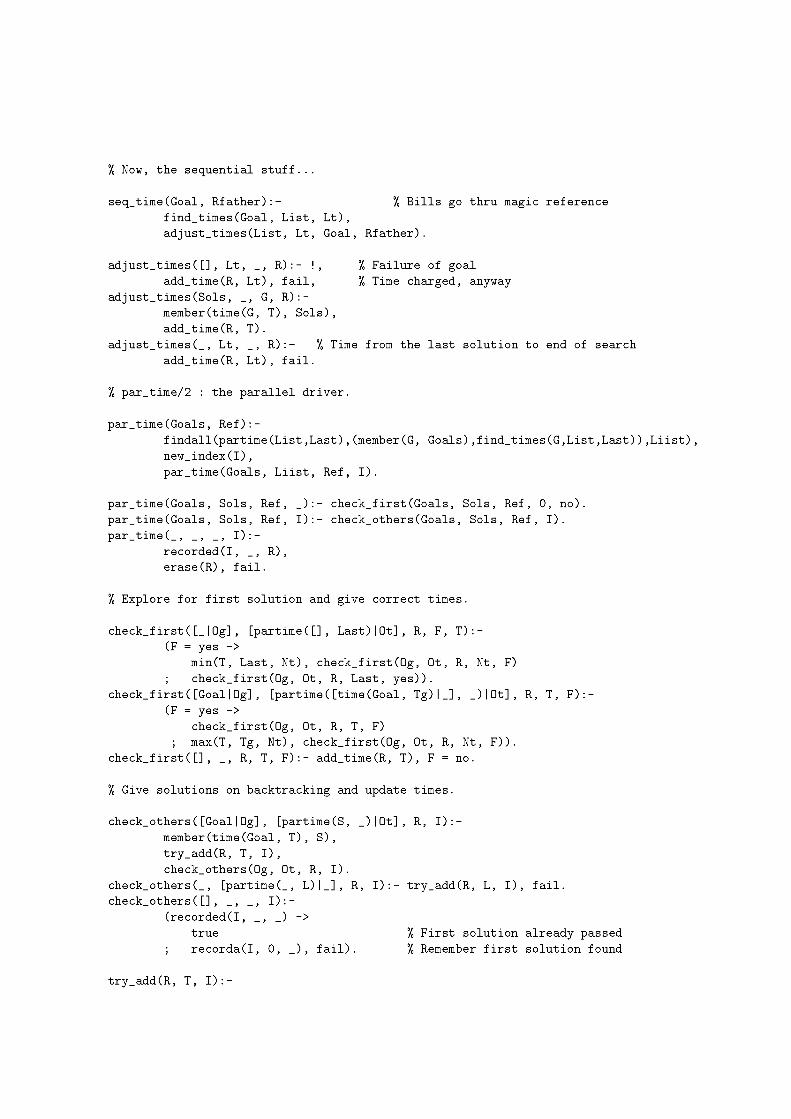
7o Now, the sequential stuff...

seq_time(Goal, Rfather):- °/0 Bills go thru magic reference

find_times(Goal, List, Lt), adjust_times(List, Lt, Goal, Rfather).

adjust_times([], Lt, _, R):- !, °/0 Failure of goal

add_time(R, Lt), fail, °/0 Time charged, anyway adjust_times(Sols, _, G, R):-

member(time(G, T), Sols),

add_time(R, T). adjust_times(_, Lt, _, R):- °/0 Time from the last solution to end of search

add_time(R, Lt), fail.

°/0 par_time/2 : the parallel driver.

par_time(Goals, Ref):-

findall(partime(List,Last),(member(G, Goals),find_times(G,List,Last)),Liist),

new_index(I),

par_time(Goals, Liist, Ref, I).

par_time(Goals, Sols, Ref, _ ) : - check_first(Goals, Sols, Ref, 0, no). par_time(Goals, Sols, Ref, I):- check_others(Goals, Sols, Ref, I). par_time(_, _, _, I):-

recordedd, _, R) , erase(R), fail.

°/0 Explore for first solution and give correct times.

check_first([_|0g], [partime([], Last)|0t], R, F, T):-(F = yes ->

min(T, Last, Nt), check_first(Og, Ot, R, Nt, F) ; check_first(Og, Ot, R, Last, yes)).

check_first([Goal|Og], [partime([time(Goal, Tg)|_], _)|0t], R, T, F):-(F = yes ->

check_first(0g, Ot, R, T, F) ; max(T, Tg, Nt), check_first(0g, Ot, R, Nt, F)).

check_first([], _, R, T, F):- add_time(R, T), F = no.

°/0 Give solutions on backtracking and update times.

check_others([Goal|Og], [partime(S, _)|0t], R, I):-

member(time(Goal, T), S),

try_add(R, T, I),

check_others(0g, Ot, R, I ) . check_others(_, [partime(_, L ) | _ ] , R, I ) : - try_add(R, L, I ) , f a i l . check_others ( [ ] , _, _, I ) : -

( r e c o r d e d d , _, _) -> true °/0 First solution already passed

; recorda(I, 0, _ ) , fail). °/0 Remember first solution found

try_add(R, T, I):-

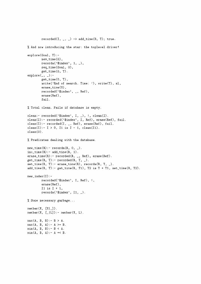
recorded(I, _, _) -> add_time(R, T); true.

7o And now introducing the star: the toplevel driver!

explore(Goal, T):-

new_time(0), recorda('$index', 1, _ ) , seq_time(Goal, 0), get_time(0, T).

explore(_, _ ) : -get_time(0, T), write('End of search. Time: ' ) , write(T), nl, erase_time(0), recorded('$index', _, Ref), erase(Ref), fail.

°/0 Total clean. Fails if database is empty.

clean:- recorded('$index', I, _ ) , !, clean(I).

clean(I) clean(I)

clean(I)

clean(O).

- recorded('$index', I, Ref), erase(Ref), fail. - recorded(I, _, Ref), erase(Ref), fail.

- I > 0, II is I - 1, clean(Il).

°/0 Predicates dealing with the database.

new_time(R):- recorda(R, 0, _ ) .

inc_time(R):- add_time(R, 1).

erase_time(R):- recorded(R, _, Ref), erase(Ref).

get_time(R, T) set_time(R, T) add_time(R, T)

- recorded(R, T, _ ) . - erase_time(R), recorda(R, T, _ ) .

- get_time(R, Tl), T2 is T + Tl, set_time(R,

new_index(I):-

recorded('$index', I, Ref), !,

erase(Ref), II is I + 1,

recorda('$index', II, _ ) .

°/0 Some necessary garbage...

member(X, [X|_]).

member(X, [_IL]):- member(X, L).

max(A, B, B)

max(A, B, A) min(A, B, B)

min(A, B, A)

- B > A.

- A >= B. - B < A.

- A =< B.

8 Conclusions

We have seen how the parallel behavior of a language can be experimented with in a sequential environment; this allows real performance of parallel programs to be tested. It should also be noted the use of standard Prolog through this paper, which makes it possible to simulate and study &-Prolog in a great variety of systems. Parallel conditions tests are easily implemented as well as a meta-interpreter. The task of constructing a simulator which give us execution times is quite tricky, but is achieved without the needing of generating traces nor explicitly implementing the control of Prolog.

All the code in this paper can be simultaneously loaded on to a sequential system, giving a environment in which parallel execution of logic programs can be experimented with. We hope this environment to be useful to all those desiring to try parallelism in their sequential computers.

9 Acknowledgements

The authors would like to thank the Swedish Institute for Computer Science (SICS) for allowing the use of SICStus-Prolog V0.5 as the starting point for the implementation of &-Prolog. We would also like to thank Maria Jose Garcia de la Banda, Francisco Bueno Carrillo, Lee Naish and Richard Warren.

References

[1] P. Biswas, S. Su, and D. Yun. A Scalable Abstract Machine Model to Support Limited-OR/Restricted AND Parallelism in Logic Programs. In Fifth International Conference and Symposium on Logic Programming, pages 1160-1179, Seattle,Washington, 1988.

[2] M. Carlsson. Sicstus Prolog User's Manual. Po Box 1263, S-16313 Spanga, Sweden, February 1988.

[3] D. DeGroot. Restricted AND-Parallelism. In International Conference on Fifth Gener­ation Computer Systems, pages 471-478. Tokyo, November 1984.

[4] G. Gupta and B. Jayaraman. Compiled And-Or Parallelism on Shared Memory Multi­processors. In 1989 North American Conference on Logic Programming, pages 332-349. MIT Press, October 1989.

[5] M. Hermenegildo. An Abstract Machine Based Execution Model for Computer Archi­tecture Design and Efficient Implementation of Logic Programs in Parallel. PhD thesis, Dept. of Electrical and Computer Engineering (Dept. of Computer Science TR-86-20), University of Texas at Austin, Austin, Texas 78712, August 1986.

[6] M. Hermenegildo. An Abstract Machine for Restricted AND-parallel Execution of Logic Programs. In Third International Conference on Logic Programming, number 225 in Lecture Notes in Computer Science, pages 25-40. Imperial College, Springer-Verlag, July 1986.

[7] M. Hermenegildo and R. I. Nasr. Efficient Management of Backtracking in AND-parallelism. In Third International Conference on Logic Programming, number 225 in LNCS, pages 40-55. Imperial College, Springer-Verlag, July 1986.

[8] M. Hermenegildo and F. Rossi. On the Correctness and Efficiency of Independent And-Parallelism in Logic Programs. In 1989 North American Conference on Logic Program­ming, pages 369-390. MIT Press, October 1989.

[9] M. Hermenegildo and F. Rossi. Non-Strict Independent And-Parallelism. In 1990 Inter­national Conference on Logic Programming, pages 237-252. MIT Press, June 1990.

[10] A.H. Karp and R.C. Babb. A Comparison of 12 Parallel Fortran Dialects. IEEE Software, September 1988.

[11] Y.-J. Lin. A Parallel Implementation of Logic Programs. PhD thesis, Dept. of Computer Science, University of Texas at Austin, Austin, Texas 78712, August 1988.

[12] K. Muthukumar and M. Hermenegildo. The CDC, UDG, and MEL Methods for Auto­matic Compile-time Parallelization of Logic Programs for Independent And-parallelism. In Int'l. Conference on Logic Programming, pages 221-237. MIT Press, June 1990.

[13] B. Ramkumar and L. V. Kale. Compiled Execution of the Reduce-OR Process Model on Multiprocessors. In 1989 North American Conference on Logic Programming, pages 313-331. MIT Press, October 1989.

[14] K. Shen and M. Hermenegildo. A Simulation Study of Or- and Independent And-parallelism. In International Logic Programming Symposium, pages 135-151. MIT Press, October 1991.

[15] P. Szeredi. Performance Analysis of the Aurora Or-Parallel Prolog System. In 1989 North American Conference on Logic Programming. MIT Press, October 1989.

[16] D.H.D. Warren. An Abstract Prolog Instruction Set. Technical Report 309, SRI Inter­national, 1983.

[17] D.H.D. Warren. The SRI Model for OR-Parallel Execution of Prolog—Abstract Design and Implementation. In International Symposium on Logic Programming, pages 92-102. San Francisco, IEEE Computer Society, August 1987.

[18] H. Westphal and P. Robert. The PEPSys Model: Combining Backtracking, AND- and OR- Parallelism. In Symp. of Logic Prog., pages 436-448, August 1987.