Experimental Investigations of NH3/CO2 Cascade and Transcritical ...
106
Experimental Investigations of NH3/CO2 Cascade and Transcritical CO2 Refrigeration Systems in Supermarkets M A N U S T A I L I K I T T H A M M A N I T Master of Science Thesis Stockholm, Sweden 2007
Transcript of Experimental Investigations of NH3/CO2 Cascade and Transcritical ...

Experimental Investigations of NH3/CO2 Cascade and Transcritical
CO2 Refrigeration Systems in Supermarkets
M A N U S T A I L I K I T T H A M M A N I T
Master of Science Thesis Stockholm, Sweden 2007
Experimental Investigations of NH3/CO2 Cascade and Transcritical CO2
Refrigeration Systems in Supermarkets
MANUSTAI LIKITTHAMMANIT
Master of Science Thesis Refrigeration Technology 2007:420 KTH School of Energy and Environmental Technology Division of Applied Thermodynamic and Refrigeration
SE-100 44 STOCKHOLM

Master of Science Thesis EGI 2007/ETT:420
Experimental Investigations of NH3/CO2 Cascade and Transcritical CO2 Refrigeration
Systems in Supermarkets
Manustai Likitthammanit
Approved
2007-06-28 Examiner
Samer Sawalha Supervisor
Björn Palm Commissioner
Installatörernas Utbildingscentrum and Sveriges Energi & Kylcentrum (IUC&SEK)
Contact person Jörgen Rogstam Laboratory Manager
Abstract An important consideration in refrigeration improvements in supermarkets, in terms of performance and environmental friendly is due to large energy consumption and refrigerant emission in supermarkets. To achieve this goal, the use of CO2 as an alternative option is being tested, with several installations already running in different European countries. The installation types running include: the indirect CO2 system, the cascade NH3/CO2, and the transcritical CO2 system. The use of CO2 as the only working fluid in the refrigeration system compared to the cascade concept means that the temperature difference in the cascade condenser will not exist which may improve the COP. This thesis is part of a project where, three refrigeration system solutions for supermarkets: R404A, NH3/CO2 cascade, and transcritical CO2 have been designed and built in the IUC laboratory at Katrineholm. The three different systems were designed to fulfill the requirements of medium size Swedish supermarket. Capacities were scaled down while keeping the load ratio comparable. The tests of these three systems were designed to simulate the conditions in a real supermarket under different weather conditions. The systems were equipped with extensive instrumentations to collect data and perform online diagnosis. Several variations of the system solutions were applied for validation and possible modifications. The tasks of this project were divided into three parts: First, transcritical CO2 refrigeration system was built, investigated, and evaluated. Its results were used to compare the NH3 system of NH3/CO2 cascade refrigeration system in terms of performance. Second, this study also compared the performance and energy consumption between the NH3/CO2 cascade system and the R404A refrigeration system.

Third, two different capacity control methods (on-off and frequency converter) of the NH3 compressor in the NH3/CO2 cascade refrigeration system were investigated and compared in terms of performance. The results of the experiment show that the COP of the investigated NH3/CO2 cascade system both at low temperature and medium temperature level is higher than R404A refrigeration system in all points of different cooling water temperatures. It also demonstrates that the COP of cascade system at low temperature level was around 20% higher than R404A system. As well with COP at medium temperature level, it is much higher than R404A system approximately 70-80%. Since a pump in R404A system was bigger than desired size, the comparison of COP without consideration of pump power at medium temperature level is also evaluated. The result shows that the COP of NH3/CO2 cascade system is still larger than R404A system about 40 – 58%. In the NH3 system, the result shows that at 20 and 25˚C of cooling water temperature, the electric input power of NH3 compressor between two different speed control types are not a big different. However, at 30˚C of cooling water temperature, NH3 compressor with on-off control ran longer time, which increased the difference of electric input power 8.34% higher than with frequency control. Thus the result shows that the COP of NH3 system with frequency control at 30˚C of cooling water temperature is 8.4% higher than with on-off control. The result also presents that the maximum COP of transcritical CO2 system was 2.5, 2.12, 1.91, and 1.54 at 15, 20, 25, and 30˚C of cooling water temperature, respectively. The performance comparison between transcritical CO2 and NH3 system shows that the COP of transcritical CO2 system is much lower than NH3 system. At 20 and 30˚C of cooling water temperature, for instance, the COP of transcritical CO2 system was lower around 48 and 51%, respectively, than NH3 system. However the evaluation of compressor data from Dorin Company demonstrates that the transcritical CO2 system with single stage compressor has higher performance than two stages compressor, which increases about 18.5 % of the COP at 30˚C of cooling water temperature. Moreover it illustrates the COP of transcritical CO2 system can be improve around 6 % when it operates without evaporator at -8˚C of evaporating temperature. Based on the experience, investigation and evaluation of the systems; NH3/CO2 cascade, R404A, and transcritical CO2 system, it can conclude that the use of frequent speed control for NH3 compressor shows higher performance than on-off control for NH3 system. In addition, using of NH3/CO2 cascade system has better solution for refrigeration in supermarket than R404A system. As well, the use of NH3 system in high stage of CO2 cascade system has higher performance than transcritical CO2 system. However, there are more important factors, such as cost of components, leakage rates, amount of charge, and heat recovery, that have to be considered to find the best solution for refrigeration in supermarket.

KTH – Stockholm, Sweden Department of Energy Technology Manustai Likitthammanit
4
ACKNOWLEDGEMENTS
The ‘CO2 in Supermarket Refrigeration’ project was initiated as an agreement between Installatörernas Utbildingscentrum and Sveriges Energi & Kylcentrum (IUC&SEK) and KTH Applied Thermodynamics and Refrigeration Division. The project was managed by IUC and financially supported from the companies Ahlsell, Huurre, AGA, WICA and ICA. This project was also financed by Energimyndigheten (STEM). This thesis work was involved in this project. First of all, I would like to express my sincere gratitude to Jörgen Rogstam and Per-Olof Nilsson from Installatörernas Utbildingscentrum and Sveriges Energi & Kylcentrum (IUC&SEK) in Katrineholm. During my time here with this thesis, Jörgen, you showed amazingly how to analysis the data, and incredibly ideas and suggestion to me. Thanks also for financial support during January to June. As well with P.O., you also showed unbelievable knowledge in practical work and from your experiences. When I worked with you, it looked like you knew everything. Also thanks for being my support, company and friend, and a lot of valuable suggestions. Furthermore, I would like to thank my supervisor, Samer Sawalha, for his help, support, advices and valuable comments. Particularly, to correct the thesis report, I knew it might make you crazy with my complicated writing. I would also like to thank my Thai friend Wimolsiri Pridasawas for her help and a lot of good suggestions at the beginning of this thesis period. Finally, I would like to thank the Swedish Refrigeration Associations (SKTF), which gave me a scholarship “Bäckströms stipendium” to work with this thesis during July to December. Manustai Likitthammanit June 2007 Stockholm, Sweden

KTH – Stockholm, Sweden Department of Energy Technology Manustai Likitthammanit
5
TABLE OF CONTENTS
ABSTRACT........................................................................................................................ 2 ACKNOWLEDGEMENTS................................................................................................ 4 TABLE OF CONTENTS.................................................................................................... 5 LIST OF FIGURES ............................................................................................................ 7 LIST OF TABLES............................................................................................................ 11 NOMENCLATURE AND DEFINITION ........................................................................ 13 1 INTRODUCTION ......................................................................................................... 15
1.1 Energy Usage in Supermarkets......................................................................... 15 1.2 Refrigerants in Supermarket ................................................................................... 17 1.3 Application of carbon dioxide in supermarket refrigeration................................... 19
1.3.1 Different system configurations for CO2 in supermarket applications ........... 20 1.3.1.1 CO2 Indirect Refrigeration Application ....................................................... 20 1.3.1.2 Cascade System with CO2............................................................................ 20 1.3.1.3 Transcritical Cycle ........................................................................................ 21
2 CO2 AS REFRIGERANT ............................................................................................. 22 2.1 Properties, Advantages and Disadvantages of CO2 ............................................... 22
3. TRANSCRITICAL CO2 CYCLE ................................................................................ 25 3.1 Fundamentals of CO2 Transcritical Cycle.............................................................. 25 3.2 Thermodynamics Losses......................................................................................... 26
4. APPLICATIONS OF CO2 TRANSCRITICAL CYCLE............................................. 29 4.1 Transcritical CO2 for Cooling Applications........................................................... 29
4.1.1 Automotive Air-Conditioning.......................................................................... 29 4.1.2 Commercial Refrigeration ............................................................................... 30 4.1.3 Transport Refrigeration.................................................................................... 31
4.2 Transcritical CO2 for Heating Applications ........................................................... 32 4.2.1 Water heating application ................................................................................ 32 4.2.2 Automotive Heat Pump ................................................................................... 33 4.2.3 Dryer ................................................................................................................ 34
5. THE EXPERIMENTAL FACILITIES......................................................................... 35 5.1 NH3/CO2 Cascade Refrigeration System............................................................... 35
5.1.1 NH3 Unit.......................................................................................................... 35 5.1.2 CO2 system...................................................................................................... 36
5.2 R404A Refrigeration System.................................................................................. 39 5.2.1 The Overall System of R404A Refrigeration System...................................... 39 5.2.2 Components ..................................................................................................... 40
5.3 Transcritical CO2 Refrigeration System................................................................. 43 5.3.1 The Overall System of Transcritical CO2 system ........................................... 43 5.3.2 Two-Stage Compressor.................................................................................... 45 5.3.3 Heat Exchangers .............................................................................................. 45 5.3.5 Oil Separator .................................................................................................... 49 5.3.6 Oil Cooler......................................................................................................... 49 5.3.7 Expansion Valve .............................................................................................. 50

KTH – Stockholm, Sweden Department of Energy Technology Manustai Likitthammanit
6
5.3.8 Heat Source...................................................................................................... 51 5.3.10 Pipes and Tube Dimension ............................................................................ 52 5.3.11 The Measurement and Controller Facilities................................................... 52 5.3.10.1 Positions of Pressure Transducers .............................................................. 53 5.3.10.2 Positions of Thermocouples........................................................................ 53 5.3.12 Safety Device ................................................................................................. 57
6. THE OVERALL SYSTEM ANALYSIS ..................................................................... 59 6.1 The Investigation and Evaluation of R404A and NH3/CO2 Cascade Refrigeration System........................................................................................................................... 59
6.1.1 The Conditions for Comparison....................................................................... 59 6.1.1.1 Freezing cabinets .......................................................................................... 59 6.1.1.2 Medium temperature cabinets....................................................................... 60 6.1.1.3 Air Temperature and relative humidity in the IUC&SEK lab ...................... 61 6.1.2 NH3/CO2 Cascade Refrigeration System........................................................ 63 6.1.3 R404A Refrigeration System........................................................................... 66
6.2 The investigation and evaluation of two different capacity control types (on-off and variable speed) of NH3 compressor in NH3/CO2 cascade refrigeration system.......... 67 6.3 The investigation and evaluation of transcritical CO2 refrigeration system .......... 67
7. EXPERIMENT RESULTS........................................................................................... 70 7.1 Results of NH3/CO2 Cascade Refrigeration System.............................................. 70
7.1.1 The System’s Temperatures............................................................................. 70 7.1.2 Cooling Capacity ............................................................................................. 73 7.1.4 The Coefficient of Performance (COP) ........................................................... 74
7.2 Results of R404A Refrigeration System................................................................. 74 7.2.1 The Systems’ Temperature .............................................................................. 74 7.2.2 Cooling Capacity ............................................................................................. 77 7.2.3 Electric Power Consumption and Energy Consumption ................................. 77 7.2.4 The Coefficient of Performance (COP) ........................................................... 78
7.3 Results of Two Capacity Control Methods of NH3 Compressor Comparison....... 78 7.3.1 The System’s Temperature .............................................................................. 78 7.3.2 Cooling Capacity, Electric Power Consumption, Energy Consumption and COP........................................................................................................................... 79
7.4 Transcritical CO2 Refrigeration System................................................................. 81 8. DISCUSSION AND CONCLUSION........................................................................... 88
8.1 Comparison between NH3/CO2 Cascade and R404A System............................... 88 8.2 Comparison of Two Speed Control Types of NH3 System.................................... 93 8.3 Comparison of Transcritical CO2 System and NH3/CO2 Cascade System........... 95
8.3.1 Comparison of Transcritical CO2 System and NH3 System........................... 99 8.3.2 Possible Improvement on Transcritical CO2 System ...................................... 99
9. REFERENCES ........................................................................................................... 104

KTH – Stockholm, Sweden Department of Energy Technology Manustai Likitthammanit
7
LIST OF FIGURES Figure 1: Typical Electricity Use of a Grocery Store in the US ............................... 16 Figure 2: Energy Usage in a Medium-Sized Supermarket in Sweden .................. 17 Figure 3: Refrigerant Distribution from a Supermarket Chain in Sweden 2003 ... 18 Figure 4: Vapour Pressure of CO2 and Other Common Refrigerants................... 22 Figure 5: Phase and Pressure -Temperature Diagram of CO2 [7] ........................ 23 Figure 6: Vapour Density of CO2 and Other Common Refrigerants [8]................ 23 Figure 7: Transcritical CO2 Cycle in Pressure-Enthalpy Diagram ......................... 25 Figure 8: Influence of Varying High Side Pressure on the COP in Transcritical Region at Different Gas Cooler Exit Temperatures [8]. ........................................... 26 Figure 9: T-s Diagram Showing Thermodynamic Losses in CO2 Refrigeration Cycle Compared to R-134a Refrigeration Cycle [7]. ................................................ 27 Figure 10: Relation between the Cooling COP and Exit Temperature of Gas Cooler Compared to R-22 and R-134a [7] ................................................................. 28 Figure 11: Components Used in FCHV and Air-Conditioning System and Schematic Diagram of the System [11] ...................................................................... 30 Figure 12: Basic Schematic Diagram of MT and LT System [12] .......................... 30 Figure 13: Sanyo CO2 Refrigeration Unit for Coca Cola Vending Machine [14] . 31 Figure 14: Sanyo’s CO2 Heat Pump Distributed in Sweden by Ahlsell [10]......... 33 Figure 15: Transcritical CO2 for Automotive Heat Pump System Tested in Audi 4A car [17]. ...................................................................................................................... 33 Figure 16: The Fluid Bed Dryer with CO2 as Refrigerant and Drawing of the Fluid Bed Dryer......................................................................................................................... 34 Figure 17: Schematic of the NH3 unit and the NH3/CO2 Cascade Refrigeration System in IUC&SEK Lab............................................................................................... 35 Figure 18: Picture of NH3 Bock Reciprocating Compressor ................................... 36 Figure 19: Picture of Cascade Condenser Heat Exchanger Installed in the Facility........................................................................................................................................... 36 Figure 20: Picture of CO2 Compressor ...................................................................... 37 Figure 21: Picture of CO2 Accumulation Tank .......................................................... 37 Figure 22: Picture of CO2 Pump.................................................................................. 38 Figure 23: Picture of Two Simulators.......................................................................... 38 Figure 24: Schematic Diagram of R404A Refrigeration System Both in Medium Temperature Level (left) and Freezing Temperature (right).................................... 39 Figure 25: Two Simulators both for Freezer and Medium Temperature Level, and another Load for Freezer .............................................................................................. 40 Figure 26: Helical Oil Separators and Copeland Scroll Compressors Used for Cooling Cabinets. ........................................................................................................... 41 Figure 27: Picture of Accumulators both for Medium Temperature Level and Freezing Temperature Level ........................................................................................ 41 Figure 28: The Brine Pump .......................................................................................... 42
KTH – Stockholm, Sweden Department of Energy Technology Manustai Likitthammanit
8
Figure 29: Picture of Bizter Compressor Used in Freezing Cabinets and ALCO Controls Oil Separators ................................................................................................. 42 Figure 30: Schematic Diagram of the Transcritical CO2 System ........................... 44 Figure 31: Picture of Transcritical CO2 system......................................................... 44 Figure 32: Picture of the Two-Stage CO2 Compressor ........................................... 45 Figure 33: Picture of the Gas Cooler .......................................................................... 46 Figure 34: Picture of the Evaporator (Cascade Condenser) ................................... 46 Figure 35: Picture of Intermediate Heat Exchanger ................................................. 47 Figure 36: Picture of Internal Heat Exchanger .......................................................... 47 Figure 37: Picture of Inside of Accumulator (left) and Accumulator (right) ........... 48 Figure 38: Picture of Small Hole for Releasing Oil from CO2 Refrigerant ............ 48 Figure 39: Picture of Inside Oil Separator (left) and Oil Separator (right) ............. 49 Figure 40: Picture of Oil Cooler.................................................................................... 50 Figure 41: Picture of Expansion Valve........................................................................ 50 Figure 42: Shut and Shut Control Used to Add Heat in the System ...................... 51 Figure 43: Water Supply for Gas Cooler and Intermediate Heat Exchanger ....... 52 Figure 44: Diagram for Evaporating Pressure Control (left), Expansion Valve Control (middle) and for Shut Control (right).............................................................. 55 Figure 45: The Display of Data on Computer Screen .............................................. 56 Figure 46: Pictures of Thermistors and Oil Pressure Alarm.................................... 57 Figure 47: Pictures of Electromechanical Pressure and Relief Valve ................... 58 Figure 48: Product Dummies and Product Temperature Measurement Point in Freezing Cabinets .......................................................................................................... 60 Figure 49: Product Dummies and Product Temperature Measurement Point in Cooling Cabinet 2 as the Example. ............................................................................. 61 Figure 50: Air Temperature in the Laboratory Set around 20 ˚C............................ 62 Figure 51: Psychometric Chart, which presents the higher humidity, the higher enthalpy. .......................................................................................................................... 62 Figure 52: The Relative Humidity in the Lab.............................................................. 63 Figure 53: Diagram of Energy Balance around the two stage CO2 compressor. 68 Figure 54: Air and Product Temperatures in Freezing Cabinet 1 of NH3/CO2 Cascade System ............................................................................................................ 70 Figure 55: Air and 2 Product Temperatures in Cooling Cabinet of NH3/CO2 Cascade System ............................................................................................................ 71 Figure 56: Operating Temperatures of the NH3/CO2 Cascade System at 20˚C of Cooling Water Temperature. ........................................................................................ 72 Figure 57: Operating Temperatures of the NH3/CO2 Cascade System at 25˚C of Cooling Water Temperature ......................................................................................... 72 Figure 58: Temperatures of Boundary Conditions in the NH3/CO2 Cascade System at 30˚C of Cooling Water Temperature ........................................................ 72 Figure 59: Operating temperatures of the R404A system with 15˚C of Cooling Water Temperature ........................................................................................................ 75 Figure 60: Operating temperatures of the R404A system with 20˚C of Cooling Water Temperature ........................................................................................................ 76

KTH – Stockholm, Sweden Department of Energy Technology Manustai Likitthammanit
9
Figure 61: Operating temperatures of the R404A system with 25˚C of Cooling Water Temperature ........................................................................................................ 76 Figure 62: Operating temperatures of the R404A system with 30˚C of Cooling Water Temperature ........................................................................................................ 77 Figure 63: Electric Power Consumption of NH3 Compressor when Compressor Was Running with Frequency and On-Off Control ................................................... 79 Figure 64: Cooling Capacities and Electric Input Powers at 25˚C of Cooling Water Temperature at Different Discharge Pressures ............................................. 81 Figure 65: Cooling Capacities and Electric Input Powers at 30˚C of Cooling Water Temperature at Different Discharge Pressures ............................................. 82 Figure 66: COP at Different Discharge Pressures at 25˚C of Cooling Water Temperature.................................................................................................................... 82 Figure 67: COP at Different Discharge Pressures at 30˚C of Cooling Water Temperature.................................................................................................................... 83 Figure 68: Cooling Capacities and Electric Input Powers at 15˚C of Cooling Water Temperature at Different Discharge Pressures ............................................. 83 Figure 69: Cooling Capacities and Electric Input Powers at 20˚C of Cooling Water Temperature at Different Discharge Pressures ............................................. 84 Figure 70: COP at Different Discharge Pressures at 15˚C of Cooling Water Temperature.................................................................................................................... 84 Figure 71: COP at Different Discharge Pressures at 20˚C of Cooling Water Temperature.................................................................................................................... 85 Figure 72: COPs of the NH3/CO2 Cascade System................................................ 89 Figure 73: COPs of the R404A System...................................................................... 89 Figure 74: The Performance Comparison of Freezer and Medium Temperature Circuits in NH3/CO2 Cascade and R404A System .................................................. 90 Figure 75: COP Comparison in Percentage of Low and Medium Temperature Circuits, NH3/CO2 Cascade is related to R404A System ....................................... 91 Figure 76: The Performance Comparison of Medium Temperature Circuit in Percentage without Consideration of Pump Power .................................................. 92 Figure 77: Total COP Comparison of NH3/CO2 Cascade and R404A Systems. 93 Figure 78: Electric Input Power Consumption for Both On-Off and Frequency Converter Control ........................................................................................................... 94 Figure 79: Ammonia unit and total system COPs with On-Off and Frequency Controls of the NH3 Compressor ................................................................................ 94 Figure 80: The plot of test’s conditions at 30 ˚C of cooling water temperature with different discharge pressures ....................................................................................... 96 Figure 81: The plot of test’s conditions at 25 ˚C of cooling water temperature with different discharge pressures ....................................................................................... 97 Figure 82: The plot of test’s conditions at 15 ˚C of cooling water temperature with different discharge pressures ....................................................................................... 98 Figure 83: The plot of test’s conditions at 20 ˚C of cooling water temperature with different discharge pressures ....................................................................................... 98

KTH – Stockholm, Sweden Department of Energy Technology Manustai Likitthammanit
10
Figure 84: The Performance Comparison between Transcritical CO2 System and NH3 System .................................................................................................................... 99 Figure 85: The Performance Comparison between Single and Two Stages CO2 Compressor from Dorin’s Compressor Data............................................................ 100 Figure 86: COPs of Single-stage Transcritical, Two-Stage Transcritical and NH3 Systems ......................................................................................................................... 101 Figure 87: Schematic Diagram of the Transcritical CO2 System without Cascade Condenser ..................................................................................................................... 102 Figure 88: COPs of Single-stage Transcritical, Two-Stage Transcritical and NH3 Systems at Evaporating Temperature of -11°C and Single-stage Transcritical at Evaporating Temperature of -8°C.............................................................................. 102

KTH – Stockholm, Sweden Department of Energy Technology Manustai Likitthammanit
11
LIST OF TABLES
Table 1: Regulation of CFC, HCFC, and HFC Refrigerants in Sweden [2] .......... 18 Table 2: Comparison for Selected Refrigerants of Required Pipe Sizes at -30 ˚C Saturated Suction Temperature and -10 ˚C Saturated Condensing Temperature [3] ...................................................................................................................................... 19 Table 3: The Primary Refrigeration Piping Consist the Following Insider Tube Diameter .......................................................................................................................... 52 Table 4: Different Cascade System Cooling Capacities at Different Cooling Water Temperature.................................................................................................................... 73 Table 5: Different Cascade System Input Powers at Different Cooling Water Temperature.................................................................................................................... 74 Table 6: Cascade System’s Coefficient of Performances at Different Cooling Water Temperature ........................................................................................................ 74 Table 7: R404A System Cooling Capacities at different Cooling Water Temperature.................................................................................................................... 77 Table 8: R404A system Electric Input Powers and Energy Consumptions at Different Cooling Water Temperatures of R404A Refrigeration System............... 77 Table 9: R404A system COPs at Different Cooling Water Temperatures ............ 78 Table 10: Products and System Temperatures of NH3/CO2 Cascade System with Frequency Control of NH3 Compressor ............................................................. 78 Table 11: Products and System Temperatures of NH3/CO2 Cascade System with On-Off Control of NH3 Compressor .................................................................... 79 Table 12: Cooling Capacities at Different Cooling Water Temperatures of the Cascade System with Frequency Control of the NH3 Compressor ....................... 79 Table 13: System’s Electric Power Consumption and Energy Consumption at Different Cooling Water Temperature of the Cascade System with Frequency Control of the NH3 Compressor................................................................................... 80 Table 14: System’s Electric Power Consumption and Energy Consumption at Different Cooling Water Temperature of the Cascade System with On-Off Control of the NH3 Compressor ................................................................................................ 80 Table 15: System’s Coefficient of Performance at Different Inlet Water Temperatures of the Cascade System with Frequency Control of the NH3 Compressor..................................................................................................................... 80 Table 16: System’s Coefficient of Performance at Different Inlet Water Temperatures of the Cascade System with On-Off Control of the NH3 Compressor..................................................................................................................... 80 Table 17: Intermediate Pressure, CO2 Mass Flow Rate and CO2 Compressor Isentropic Efficiency Results at 15˚C of Cooling Water Temperature at Different Discharge Pressures ..................................................................................................... 85

KTH – Stockholm, Sweden Department of Energy Technology Manustai Likitthammanit
12
Table 18: Capacities of system’s heat exchangers at 15˚C of Cooling Water Temperature at Different Discharge Pressures......................................................... 85 Table 19: Intermediate Pressure, CO2 Mass Flow and CO2 Compressor Results at 20˚C of Cooling Water Temperature in Different Discharge Pressures............ 86 Table 20: Capacities in Each Component at 20˚C of Cooling Water Temperature in Different Discharge Pressures ................................................................................. 86 Table 21: Intermediate Pressure, CO2 Mass Flow and CO2 Compressor Results at 25˚C of Cooling Water Temperature in Different Discharge Pressures............ 86 Table 22: Capacities in Each Component at 25˚C of Cooling Water Temperature in Different Discharge Pressures ................................................................................. 86 Table 23: Intermediate Pressure, CO2 Mass Flow and CO2 Compressor Results at 30˚C of Cooling Water Temperature in Different Discharge Pressures............ 87 Table 24: Capacities in Each Component at 30˚C of Cooling Water Temperature in Different Discharge Pressures ................................................................................. 87
KTH – Stockholm, Sweden Department of Energy Technology Manustai Likitthammanit
13
NOMENCLATURE AND DEFINITION
HVAC: Heating, Ventilation and Air-conditioning CFC: (Chlorofluorocarbon) any of various halocarbon compounds consisting of carbon, hydrogen, chlorine, and fluorine. HCFC: (Hydro chlorofluorocarbons) are halogenated compounds containing carbon, hydrogen, chlorine and fluorine. They have shorter atmospheric lifetimes than CFCs and deliver less reactive chlorine to the stratosphere where the “ozen layer” is found. Annex 31: It is a project established under the auspices of the International Energy Agency’s (IEA) Energy Conservation in Buildings and Community Systems Programme. It examines how energy and life cycle assessment (LCA) tools and methods can be used to reduce the energy-related impact of buildings on interior, local and global environments. Ozone Depletion Potential (ODP) [2] – The ODP of a chemical compound is the relative amount of degradation to the ozone layer it can cause, with trichlorofluoromethane (R-11) being fixed at an ODP of 1.0. Global Warming Potential (GWP) [3] – The GWP is a measure of how much a given mass of greenhouse gas is estimated to contribute to global warming. It is a relative scale which compares the gas in question to that of the same mass of carbon dioxide (whose GWP is by definition 1). A GWP is calculated over a specific time interval and the value of this must be stated whenever a GWP is quoted or else the value is meaningless. COP: Coefficient of performance LCCP: Life Cycle Climate Performance Q& : Cooling capacity (kW) m& : Refrigerant mass flow rate (kg/s) Cp : Specific heat (kJ/ kg*K) dT : Temperature difference (ºC) dh : Enthalpy difference (kJ/kg)
vη : Volumetric efficiency of the compressor (-)
isη : Isentropic efficiency (-)

KTH – Stockholm, Sweden Department of Energy Technology Manustai Likitthammanit
14
sV& : Swept volume flow (m3/h)
inρ : Density of the refrigerant at the inlet to the compressor (kg/m3)
srV& : Compressor displacement volume n : Compressor speed (rpm)
rn : Compressor rated speed (rpm)
outletP : Discharge pressure (bar)
inletP : Suction pressure (bar)
lossesη : Compressor thermal efficiency (-)
eleccompE ,& : Compressor electrical power (kW)
shaftcompE ,& : Compressor mechanical power (kW)
compdh : Compressor enthalpy difference (kJ/kg)
pumpE& : Pump power (kW) I : Current (A) V : Voltage (V) Pr: Product dummies in cabinets F: Frequency converter control On-Off: On-Off control Subscripts W: Water side Trans: Transcritical system cascad: Cascade system Pierre: Based on Pierre’s correlation comp: Compressor shaft: Mechanical shaft work evap: evaporator losses: Efficiency losses in the compressor sim: Simulator is: isentropic in: Inlet out: Outlet

KTH – Stockholm, Sweden Department of Energy Technology Manustai Likitthammanit
15
1 INTRODUCTION Supermarkets consume a lot of energy, particularly in the refrigeration part. In addition, supermarkets also have large refrigerant emissions, which is the second refrigerant emission source after mobile air-conditioning. Thus, development of an efficient and environmentally friendly refrigeration system in supermarkets will help reducing the energy consumption and the impact on the environment. To decrease environmental impact from refrigeration, the use of natural refrigerants, such as water, air, hydrocarbon, ammonia, and CO2, instead of CFC, HCFC, and HFC has been increasing. However, for supermarkets, water and air have not been interesting alternatives because of high freezing point for the water and low theoretical efficiency of Brayton cycle for air. Ammonia, hydrocarbons, and CO2 have a broader range of application, and are used in much more conventional systems. Among these, CO2 is the only non-flammable and non-toxic fluid that can also operate in a vapor compression cycle below 0˚C. Thus, CO2 has the potential to offer environmental and personal safety in a system. There are also many advantages using CO2 as refrigerant, such as low refrigerant cost, low pressure and temperature drops, low volume flow rate, high vapor density, good heat transfer characteristics, and good compatibility with oil. Furthermore, using CO2 as refrigerant in transcritical refrigeration system can avoid a different temperature in cascade condenser of NH3/CO2 cascade system since CO2 will absorb heat from CO2 in sub-cycle directly without cascade condenser. Consequently, the use CO2 refrigeration system in supermarket has become potential alternative for conventional solutions.
1.1 Energy Usage in Supermarkets From Annex 31 [1], supermarkets are the most intensive buildings in the commercial sector that consume a lot of energy. It is estimated that supermarkets in industrialized countries consume 3-5% of the total electricity usage. In the USA, this accounts for about 2-3 million kWh per year for supermarkets with about 3700-5600 m2 sales area. In groceries, the national average electricity intensity is estimated of 565 kWh/m2 per year.

KTH – Stockholm, Sweden Department of Energy Technology Manustai Likitthammanit
16
As for Sweden, supermarkets consume about 3% of the electricity consumption (1,800 million kWh/year) [2]. The total energy consumption in a hypermarket (about 7000 m2) is about 326 kWh/m2 per year while the total energy consumption in small neighborhood shops (about 600 m2) is about 471 kWh/m2 per year [2]. Figure 1 presents typical electricity use of a grocery store in the US. There are six main electricity uses in a supermarket: for refrigeration, lighting, ventilation, cooling, heating, and cooking. Electricity use in refrigeration is the highest which is around 39% [2]. In the case of a medium-sized supermarket in Sweden, refrigeration consumes the highest of the electricity which is approximately 47% compared with lighting (27%), HVAC (13%), kitchen (3%), and outdoor (5%) [2]. Figure 2 shows the typical electricity use of a grocery store in US.
Refrigeration 39%
Lighting23%
Cooling11%
Ventilation4%
Heating13%
Miscellaneous3%
Water Heating2% Cooking
5%
Refrigeration Lighting Cooling VentilationHeating Miscellaneous Water Heating Cooking
Figure 1: Typical Electricity Use of a Grocery Store in the US

KTH – Stockholm, Sweden Department of Energy Technology Manustai Likitthammanit
17
refrigeration , 47%
Lighting, 27%
HVAC, 13%
kitchen, 3%
Outdoor, 5%
Other, 5%
refrigeration Lighting HVAC kitchen Outdoor Other
Figure 2: Energy Usage in a Medium-Sized Supermarket in Sweden Moreover, it is estimated that the refrigerant losses from refrigeration in supermarkets are annually around 15-30 % of total charge which is the second refrigerant emission source after mobile air-conditioning [1]. Consequently, improvements on refrigeration system in supermarkets can help to cut the energy consumption and reduce the impact on the environment from refrigerant loss.
1.2 Refrigerants in Supermarket From the prediction [3], the average global temperature will be increased between 1.5 and 4.5˚C in the next 100 years. The cause of global warming is mainly from the emission of greenhouse gases into the Earth’s atmosphere. Commercial refrigeration, including supermarket has large emissions by sector which is around 37% of the worldwide refrigerant emissions [2]. Refrigeration applications contributions to global warming are classified as direct and indirect. For direct contribution in supermarket applications, greenhouse gas emissions occur through the leakage of HFC’s used in refrigeration systems for display and storage of food. The indirect contribution comes from the production of CO2 gas through energy consumption where supermarkets are large consumers of electricity. According to the effect of the CFCs and HCFCs on the ozone layer, discovered during the 1970s, the usage of ozone-depleting CFC refrigerants has been banned by 1990s, followed by the phase-out of HCFCs in the early 2000’s. However, the use of the HFCs is still legal and commonplace.
KTH – Stockholm, Sweden Department of Energy Technology Manustai Likitthammanit
18
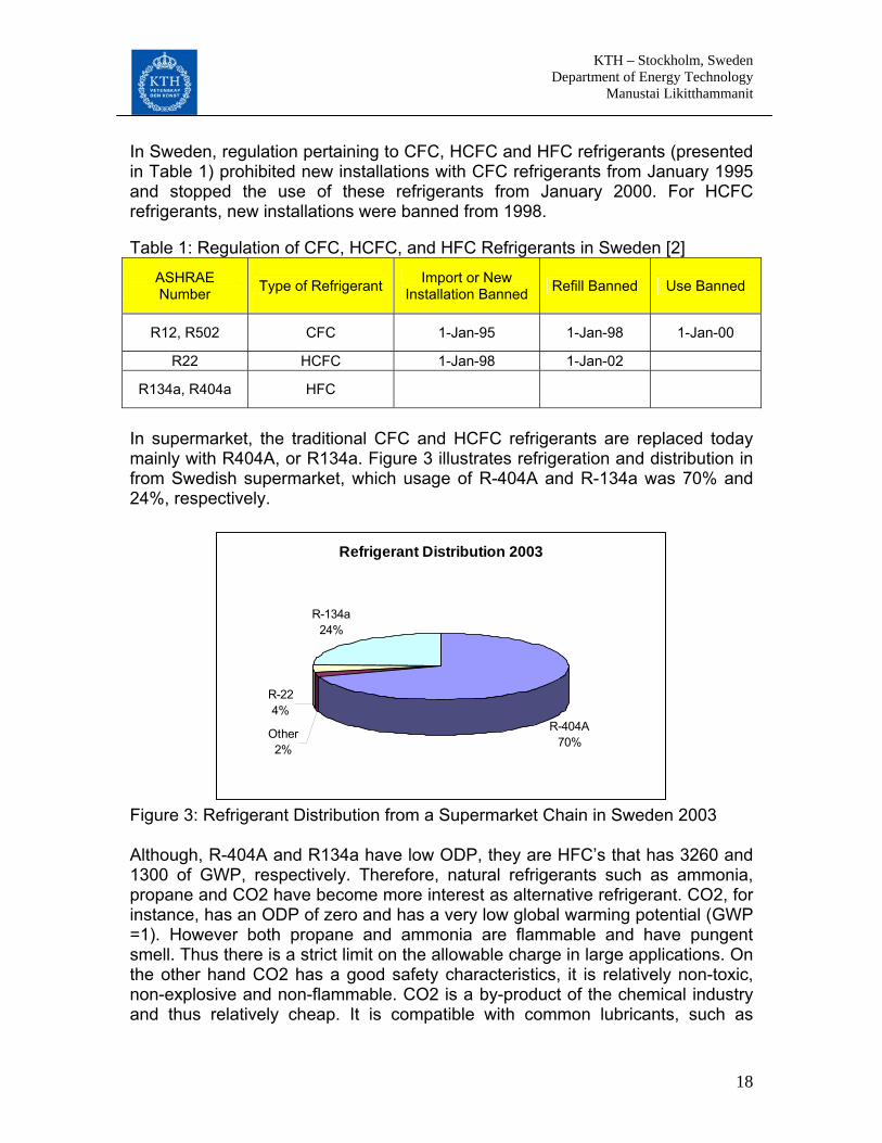
In Sweden, regulation pertaining to CFC, HCFC and HFC refrigerants (presented in Table 1) prohibited new installations with CFC refrigerants from January 1995 and stopped the use of these refrigerants from January 2000. For HCFC refrigerants, new installations were banned from 1998. Table 1: Regulation of CFC, HCFC, and HFC Refrigerants in Sweden [2]
ASHRAE Number Type of Refrigerant Import or New
Installation Banned Refill Banned Use Banned
R12, R502 CFC 1-Jan-95 1-Jan-98 1-Jan-00
R22 HCFC 1-Jan-98 1-Jan-02
R134a, R404a HFC
In supermarket, the traditional CFC and HCFC refrigerants are replaced today mainly with R404A, or R134a. Figure 3 illustrates refrigeration and distribution in from Swedish supermarket, which usage of R-404A and R-134a was 70% and 24%, respectively.
Refrigerant Distribution 2003
R-404A70%
Other2%
R-224%
R-134a24%
Figure 3: Refrigerant Distribution from a Supermarket Chain in Sweden 2003 Although, R-404A and R134a have low ODP, they are HFC’s that has 3260 and 1300 of GWP, respectively. Therefore, natural refrigerants such as ammonia, propane and CO2 have become more interest as alternative refrigerant. CO2, for instance, has an ODP of zero and has a very low global warming potential (GWP =1). However both propane and ammonia are flammable and have pungent smell. Thus there is a strict limit on the allowable charge in large applications. On the other hand CO2 has a good safety characteristics, it is relatively non-toxic, non-explosive and non-flammable. CO2 is a by-product of the chemical industry and thus relatively cheap. It is compatible with common lubricants, such as

KTH – Stockholm, Sweden Department of Energy Technology Manustai Likitthammanit
19
elastomers mineral oils, polyol esters (POE), polyalphaolefines (PAO), polyalkylene glycols (PAG) and alkyl naphthenes (AN), and common construction materials. Furthermore, due to high volumetric capacity, the size of components and piping system are quite small compared to ammonia and R-404A‘s, that shows in table 2, which results in minimum charge of CO2 system and make it almost an ideal fluid to be used in the refrigerated space with relatively large quantities. Table 2: Comparison for Selected Refrigerants of Required Pipe Sizes at -30 ˚C Saturated Suction Temperature and -10 ˚C Saturated Condensing Temperature [3]
Refrigerant R-404A R-717 R-744
Capacity 150 kW 150 kW 150 kW
Circuit penalty 1.4 K 1.5 K 0.8 K
Velocity 11.3 m/s 25.6 m/s 7.7 m/s
Diameter 101.6 mm 72.6 mm 50.8 mm
Dry suction Line
Area 8107 mm2 4139 mm2 2026 mm2
Velocity 0.6 m/s 0.3 m/s 1.1 m/s
Diameter 38.1 mm 25.4 mm 25.4 mm Liquid Line
Area 1140 mm2 506 mm2 506 mm2 This leaves carbon dioxide as the only natural refrigerant candidate to be used in supermarket refrigeration.
1.3 Application of carbon dioxide in supermarket refrigeration Since the revival of CO2 as alternative refrigerant, most of the research work has been focusing on the usage of carbon dioxide in mobile air conditioning and heat pump application. For instance, a group in Europe has been founded in July 2000 with the name of Carbon Dioxide Interest Group (c-dig) initially to share the knowledge for industrial applications. Also IIR-Gustav Lorentzen series of conferences for natural refrigerants show the growing research interests in the field.
KTH – Stockholm, Sweden Department of Energy Technology Manustai Likitthammanit
20
For supermarket refrigeration applications, the three main solutions where CO2 is applied are the indirect cascade and transcritical systems.
1.3.1 Different system configurations for CO2 in supermarket applications
1.3.1.1 CO2 Indirect Refrigeration Application In commercial refrigeration, the main technology that was commercially utilized was to use CO2 as secondary refrigerant in indirect systems for freezing temperature applications. CO2 has been successfully used in indirect system solution, the pumping power needed is quite small compared to conventional brine system, and this is due to the small CO2 volume flow rate and the resulting low pressure drop. The small volume flow rate is due to the phase changing process on the CO2 side which also contributes to improving heat transfer on the refrigerant side compared to the cases with non-phase changing fluids, such as conventional brines.
1.3.1.2 Cascade System with CO2 To eliminate the temperature difference in the extra heat exchanger needed to transfer heat to CO2 in the indirect loop, a system using CO2 as refrigerant in low stage of a cascade system has been developed. A cascade refrigeration system with CO2 in the low temperature stage and other refrigerants, such as ammonia, propane, and R-404A, in the high stage is an interesting solution that has been tested in several supermarkets. In Denmark, for instance, propane/CO2 system was installed in small supermarket, “Dagli Brugsen”, in Odense, Denmark in 2000[5]. Propane was used at the high temperature level (-14/25˚C), while CO2 is used at the low temperature level (-32/-10˚C).The system operated at around 21 kW for cooling and 10 kW or freezing. This project illustrated very interesting results that energy consumption of propane/CO2 is less than conventional R-404A systems. Although investment cost of propane/CO2 was between 12-20% higher, it can be decrease to around 10% if the system is larger (approx 60 kW for cooling and 30 kW for freezing). In Netherlands, the first NH3/CO2 cascade system, which has NH3 as primary refrigerant and CO2 as secondary refrigerant, is installed in supermarket in Bunschoten[6]. It operates in two parallel cascade heat exchangers where condensing temperature of CO2 cycle is -12˚C and evaporating temperature of

KTH – Stockholm, Sweden Department of Energy Technology Manustai Likitthammanit
21
NH3 is -16˚C. The NH3 condenses at a temperature of 10 C above the ambient temperature. The two NH3 screw compressors can operate in range from 20 kW to 76.4 kW as one of the compressors is frequency controlled. For CO2 circuit, direct expansion and a CO2 compressor provides the freezing section with CO2 of 10.8 kW, while in cooling section, pump is used to circulate CO2 providing cooling capacity of 63.7 kW. The result shows that the annual energy saving is 13-18% compared to R-404A. Moreover investment costs are expected to be lower than those of a conventional system due to the governmental subsidies. However without these subsidies the investment was 28% higher with a payback period of approximately eight years due to lower operational cost.
1.3.1.3 Transcritical Cycle The temperature difference that exists in the cascade condenser in the cascade system will decrease the evaporating temperature on the high stage and will reduce system’s COP. An efficient transcritical CO2 system will by-pass the need for cascade condenser which may improvement the COP. During operation at high ambient air temperature the CO2 system will operate in transcritical cycle most of the time heat rejection then takes place by cooling the compressed fluid at supercritical high-side pressure.
KTH – Stockholm, Sweden Department of Energy Technology Manustai Likitthammanit
22
2 CO2 AS REFRIGERANT
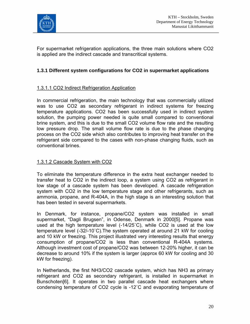
2.1 Properties, Advantages and Disadvantages of CO2 According to ASHRAE standard 34, CO2 is in a group A1 which is the group of the refrigerants that does not have an identified toxicity at concentration below 400 ppm, thus it has good safety characteristics. From environmental point of view, it has no ODP and GWP of 1. Figure 4 presents vapour of CO2 and other common refrigerants. CO2 vapor pressure is much higher than other refrigerants and its volumetric refrigeration capacity (22,545 kJ/ m3 at 0˚C) is 3-10 times higher than other refrigerants, such as R410A, R404A, R407C, R22, R134a, R12, Propane, and Ammonia [8].
Figure 4: Vapour Pressure of CO2 and Other Common Refrigerants. Figure 5 presents phase and pressure – temperature diagram of CO2. The critical pressure and temperature of CO2 are 73.8 bar and 31.1˚C, respectively. Its temperature and pressure for the triple point are -56.6˚C and 5.2 bar, respectively.

KTH – Stockholm, Sweden Department of Energy Technology Manustai Likitthammanit
23
Figure 5: Phase and Pressure -Temperature Diagram of CO2 [7] Owing to the low critical temperature, CO2 will be much closer to the critical point than with conventional refrigerants. The density of CO2, as shown in Figure 6, changes rapidly with temperature near the critical point, and the density ratio of CO2, which is used to determine the flow pattern and heat transfer coefficient, is much smaller than other refrigerants.
Figure 6: Vapour Density of CO2 and Other Common Refrigerants [8]. CO2 is an inert gas, hence the choice of metallic materials for piping and components does not generally present a problem, provided dry CO2 is used and the maximum design pressures can be handled by system components. Heat transfer of carbon dioxide is one interesting characteristic as it is superior to other refrigerants. High vapor density, low surface tension by one order of magnitude, and low vapor viscosity considerably influence the convective and nucleate boiling characteristics of CO2. These results in heat transfer coefficient

KTH – Stockholm, Sweden Department of Energy Technology Manustai Likitthammanit
24
of CO2 that are greater than those of conventional refrigerant by 2-3 times at the same saturation temperature while its two phase pressure drops are significantly smaller [7]. The low pressure drop and the low volume flow rate, result in lower the energy consumption of the pump in the indirect circuit which will give CO2 a major advantage compared to brine based systems. Moreover, another advantage of CO2 as refrigerant is the small components and pipes’ diameter that can be used; this is due to its high working pressure and low pressure drop. This has favored carbon dioxide in application which requires compact design due to limited space availability. CO2 is also a chemical non-active substance and most of oils do not react with it, bigger concern is the reaction with the refrigerant in the high stage in case of mixing. Good solubility in the refrigerant is a good characteristic of oil which means good transport of oil and oil separation may not needed. An issue to consider with CO2 lubrication is that usually oils are lighter than CO2 and if they are not miscible in it they will float on the surface thus will be hard to separate. The amount of oil needed for CO2 compressor is much smaller than that is needed for an ammonia compressor which saves in the running cost. Using an oil free compressor is an option, the installation cost is high but it still saves in the oil system and the price of the oil itself, but the maintenance cost is expected to be higher. From construction point of view, a disadvantage with CO2 as a refrigerant is the high working pressure. This pressure is much higher than that of the other natural and synthetic refrigerants, as explained above. Therefore, stronger components must be designed to handle CO2 in the transcritical cycle. Industries, for instance, have already started succeeding in coping with the related problems providing proper safety strategies and components design. Furthermore, CO2 is denser than air and it can displace the oxygen in the space. Both characteristics can be dangerous in case of leakage, especially in reduced spaces. Symptoms associated with the inhalation of air containing CO2 are presented in [19]. Detection and good ventilation systems should be placed in a plant which uses CO2 as refrigerant. If any liquid CO2 leakage happens in the system, it will pass through its triple point (-56.6ºC at 5.2 bar), ‘dry ice’ will appear and the leakage may be sealed by itself. In spite of being a good factor from safety point of view, it represents a risk in case of the need to release CO2 liquid through a relief valve [19].

KTH – Stockholm, Sweden Department of Energy Technology Manustai Likitthammanit
25
3. TRANSCRITICAL CO2 CYCLE
3.1 Fundamentals of CO2 Transcritical Cycle Figure 7 demonstrates transcritical CO2 cycle in pressure and enthalpy diagram. The CO2 system will operate above critical point (31.1˚C and 73.8 bar) in the transcritical region. In the transcritical region, the temperature is independent of the pressure and there is no saturation condition. Moreover, it is not only temperature that has mainly effect on the specific enthalpy but also the pressure.
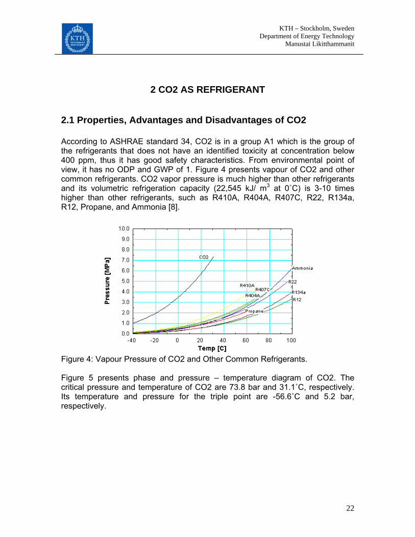
Figure 7: Transcritical CO2 Cycle in Pressure-Enthalpy Diagram For the COP in transcritical region, COP value in transcritical area is a function of discharge pressure and gas cooler outlet temperature. For every gas cooler outlet temperature (Tout), there is a discharge pressure that gives a maximum or optimum value of COP in transcritical area, as shown in Figure 8. At 35˚C of Tout, for instance, the theoretical maximum COP is reached at pressure of 85.9 bar, while at 45˚C, the optimum is at 109.8 bar [8].
KTH – Stockholm, Sweden Department of Energy Technology Manustai Likitthammanit
26
Figure 8: Influence of Varying High Side Pressure on the COP in Transcritical Region at Different Gas Cooler Exit Temperatures [8]. This kind of system is most suitable for cold climate or where cold heat sinks are available. In this case, the operation of such plants will be mostly in the sub-critical region. However, if hot water production is needed then it is possible to effectively utilize the transcritical side of the cycle for hot water production, which will improve the cycle’s overall efficiency. When the ambient temperature reduces so the plant will operate in subcritical region, by-pass must be used in order to eliminate the first expansion device which is the one that controls the discharge pressure. It will not be needed in this operating condition, and the receiver that follows that expansion device will be accumulating condensate from the condenser (gas cooler).
3.2 Thermodynamics Losses In transcritical cycle, there are two main thermodynamic losses, heat rejection loss and throttling loss. The larger throttling loss in refrigeration cycle depends on temperature before and after throttling device, and also by refrigerant properties. Figure 9 represents the average temperature of CO2 in the heat rejection side is higher compared to R-134a.

KTH – Stockholm, Sweden Department of Energy Technology Manustai Likitthammanit
27
Figure 9: T-s Diagram Showing Thermodynamic Losses in CO2 Refrigeration Cycle Compared to R-134a Refrigeration Cycle [7]. When CO2 is used in hot water heat pump applications, the thermodynamics loss can be reduced. The temperature curve of the cooled CO2 refrigerant matches the heating-up curve of water better than in the case of R-134a. For cooling CO2 system, the thermodynamic loss can be minimized by allowing the CO2 exit temperature from the gas cooler to approach the air or water inlet temperature as closely as possible. Due to high heat rejection and throttling losses, the cooling COP of CO2 system is very sensitive to the exit temperature of the gas cooler. Figure 10 shows relation between the cooling COP and Exit Temperature of gas cooler compared to R-22 and R-134a.

KTH – Stockholm, Sweden Department of Energy Technology Manustai Likitthammanit
28
Figure 10: Relation between the Cooling COP and Exit Temperature of Gas Cooler Compared to R-22 and R-134a [7] However, there are some methods to limit the thermodynamic losses, such as usage of two stages compression cycle with inter-cooler. There also have been several research works to increase the performance of cooling system, such as the use of internal heat exchanger, multi-stage expansion, and ejector, as can be seen in next chapter. Consequently, although, there is a lack of efficiency of theoretical transcritical CO2 cycle, the transcritical CO2 may still compete with other refrigerant.
KTH – Stockholm, Sweden Department of Energy Technology Manustai Likitthammanit
29
4. APPLICATIONS OF CO2 TRANSCRITICAL CYCLE
4.1 Transcritical CO2 for Cooling Applications
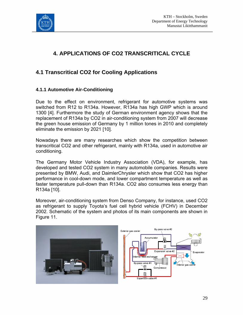
4.1.1 Automotive Air-Conditioning Due to the effect on environment, refrigerant for automotive systems was switched from R12 to R134a. However, R134a has high GWP which is around 1300 [4]. Furthermore the study of German environment agency shows that the replacement of R134a by CO2 in air-conditioning system from 2007 will decrease the green house emission of Germany by 1 million tones in 2010 and completely eliminate the emission by 2021 [10]. Nowadays there are many researches which show the competition between transcritical CO2 and other refrigerant, mainly with R134a, used in automotive air conditioning. The Germany Motor Vehicle Industry Association (VDA), for example, has developed and tested CO2 system in many automobile companies. Results were presented by BMW, Audi, and DaimlerChrysler which show that CO2 has higher performance in cool-down mode, and lower compartment temperature as well as faster temperature pull-down than R134a. CO2 also consumes less energy than R134a [10]. Moreover, air-conditioning system from Denso Company, for instance, used CO2 as refrigerant to supply Toyota’s fuel cell hybrid vehicle (FCHV) in December 2002. Schematic of the system and photos of its main components are shown in Figure 11.

KTH – Stockholm, Sweden Department of Energy Technology Manustai Likitthammanit
30
Figure 11: Components Used in FCHV and Air-Conditioning System and Schematic Diagram of the System [11]
4.1.2 Commercial Refrigeration For commercial refrigeration, CO2 is used mostly as secondary refrigerant in indirect systems, particularly in Scandinavian countries. In Sweden, for instance, by the year 2002, there are about 60 plants running with capacities ranging from 10 to 280 kW [7]. However, for transcritical CO2 system in commercial applications, many systems have been installed in northern Europe. For instance, on November 25, 2004, the first hypermarket in Switzerland using CO2 direct expansion system for both medium (MT) and low temperature (LT) refrigeration was opened. It uses three multi compressor refrigeration systems, refrigerated display cases totaling sales run of 180 meters, nine cold rooms (200 m2 base area), and five walk-in freezers (around 90 m2 base area). The basic diagram of the system is presented in Figure 12.
Figure 12: Basic Schematic Diagram of MT and LT System [12] The low temperature system is designed as cascade system, which has 28 kW of cooling capacity. For the medium temperature system, it is split between two refrigeration racks of identical capacities; it has 322 kW of cooling capacity. On the other hand, 472 kW of heat is rejected to ambient air in a CO2 gas cooler of V-block configuration. The result shows that the CO2 refrigeration system consumes less energy than R404A for out door air temperatures below 28˚C. At 35˚C, the energy consumption is 13% higher for the CO2 system. Capatal investment for this transcritical CO2 system is currently higher than R404A direct expansion system [12].

KTH – Stockholm, Sweden Department of Energy Technology Manustai Likitthammanit
31
While in light commercial application, such as the vending machine, shown in Figure 13, CO2 is becoming an interesting alternative. The Coca Cola Company has announced during the one-day conference “Refrigerants, Naturally”, “CO2- based refrigeration is currently the best option for the global needs of Coca-Cola’s sales and marketing equipment”, (cooling Coca Cola). According to a publication of Sanyo [14], it described a comparison between a transcritical CO2-refrigeration cycle and R-134a designed for Coca Cola vending machines. For this project, the CO2-compressor, which is of the hermetic 2-stage rolling piston design, and a combined gas cooler-intercooler as well as a suction line heat exchanger (SLHX), is used. The system worked under the ambient condition of 32.2˚C and 65 % of humidity. The result illustrated that the energy consumption in the vending machine is claimed to be 17% less than in original R-134a vending machines under actual field tests [14]. Moreover, tests done by Denfoss, have been published in 2004 at the IIR-Nature Working Fluids Conference in Glasgow [15]. In this project, results show that the use of transcritical CO2 system can save the energy by around 18% and 37% of double door cooler and vending machine, respectively, compared to the baseline HFC-technology including the consumption of 2 fans and lights at the ambient condition of 32˚C and 65% of humidity. In this ambient condition, the optimum discharge pressure is between 85 and 95 bar.
Figure 13: Sanyo CO2 Refrigeration Unit for Coca Cola Vending Machine [14]
4.1.3 Transport Refrigeration CO2 was used as refrigerant for transportation in ships until 1950’s, and then it was gradually phased out due to the technical problems of the high pressure and low critical temperature, also the discovery of new refrigerants at that time contributed to undermining the development in CO2 side. However, today, CO2 is renewed in the area of transport again with two main reasons. First, it is because of high density and volumetric refrigerating of CO2 at low temperatures, compared to alternatives such as hydrocarbons or ammonia, which allows the design of compact systems. Second, the use of CO2 is the worldwide availability and the regulation of HFC fits well with the global nature of the transport refrigeration industry.
KTH – Stockholm, Sweden Department of Energy Technology Manustai Likitthammanit
32
According to Man-Hoe Kim et al’s paper [7], the test results on a prototype CO2 system for truck refrigeration gave COP data that matched equally sized systems using R-502 and R-507. From the prediction of a Danish study [6], the performance of refrigerating systems for transport containers resulted with COP values that are 15–20% below those of R-134a systems, not including the effects of differences in compressor efficiency and refrigerant-side pressure drops. Furthermore, the research by Jakobsen and Neksa [10] shows very similar COP values in freezing mode for CO2 and R-134a over the full range of ambient temperature. In cooling mode, the excess capacity is much greater with R-134a than with CO2 due to differences in refrigerant properties. When the influence on COP by suction throttling or cylinder unloading was included, the estimated COP in freezing mode became slightly (3–10%) higher for the CO2 system than for the R-134a system. One problem with CO2 may be the very high compressor discharge temperature for freezing operation at high ambient temperature.
4.2 Transcritical CO2 for Heating Applications According to the thermodynamic properties of CO2 that there is high heat rejection to heat to the heat sink and matching of cure between CO2 and cooling media, it lets CO2 to be favorable for heating application. There are many heating applications that use CO2 as refrigerant and most of them have been already applied commercially, such as heat pump for auto mobile, residential heating, and water heating.
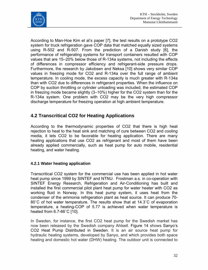
4.2.1 Water heating application Transcritical CO2 system for the commercial use has been applied in hot water heat pump since 1999 by SINTEF and NTNU. Frostman a.s. in co-operation with SINTEF Energy Research, Refrigeration and Air-Conditioning has built and installed the first commercial pilot plant heat pump for water heater with CO2 as working fluid in Norway. In this heat pump system, it uses heat from the condenser of the ammonia refrigeration plant as heat source. It can produce 70-80˚C of hot water temperature. The results show that at 14.3˚C of evaporation temperature, a heating-COP of 5.77 is achieved when water temperature is heated from 6.7-66˚C [10]. In Sweden, for instance, the first CO2 heat pump for the Swedish market has now been released by the Swedish company Ahlsell. Figure 14 shows Sanyo’s CO2 Heat Pump Distributed in Sweden. It is an air source heat pump for hydraulic heating systems, developed by Sanyo, and which provides both space heating and domestic hot water (DHW) heating. The outdoor unit is connected to
KTH – Stockholm, Sweden Department of Energy Technology Manustai Likitthammanit
33
a specially designed storage tank, where the DHW is circulated in two coils placed inside the storage tank. The heat pump, which is capacity-controlled by a variable-speed control (inverter), is claimed to deliver 4.5 kW of heat capacity down to an outdoor air temperature of -15 °C, it heats the water up to +70 °C [10].
Figure 14: Sanyo’s CO2 Heat Pump Distributed in Sweden by Ahlsell [10]
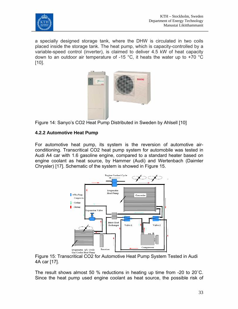
4.2.2 Automotive Heat Pump For automotive heat pump, its system is the reversion of automotive air-conditioning. Transcritical CO2 heat pump system for automobile was tested in Audi A4 car with 1.6 gasoline engine, compared to a standard heater based on engine coolant as heat source, by Hammer (Audi) and Wertenbach (Daimler Chrysler) [17]. Schematic of the system is showed in Figure 15.
Figure 15: Transcritical CO2 for Automotive Heat Pump System Tested in Audi 4A car [17]. The result shows almost 50 % reductions in heating up time from -20 to 20˚C. Since the heat pump used engine coolant as heat source, the possible risk of

KTH – Stockholm, Sweden Department of Energy Technology Manustai Likitthammanit
34
extended heating up time for the engine was of some concern. Measurements presented the added load on the engine by the heat pump compressor, the heating-up time was in fact slightly reduced even when heat was absorbed from the coolant circuit [17]. Moreover, according to Tamura’s et al paper [19], the transcritical CO2 heat pump for medium-sized car is successfully developed. The transcritical CO2 heat pump is compared with R134a system. With the use of micro tubes for the indoor and outdoor heat exchangers and double micro tube for the water-refrigerant heat exchanger, the result shows that the COP ratio between transcritical CO2 and R134a heat pump is 1.31. Transcritical CO2 heat pump is also tested for American military vehicles. It is compared with R134 heat pump with different ambient temperatures (-10 to 20˚C) and indoor temperature range -10 to 20˚C. The mass flow is constant over the indoor (0.134 m3/s) and outdoor coils (0.434 m3/ s) with compressor speed at 950 rpm. The results show that the capacity can be increased with increasing of high side pressure; engine heat can be used exclusively to reduce emission during startup instead of being diverted immediately for cabin comfort; steady state capacity is not significantly degraded by low ambient temperature [18].
4.2.3 Dryer Another interesting application of transcritical CO2 cycle is heat pump dryer. An example is a prototype fluidised bed heat pump dryer with CO2 as refrigerant, which is built at the Dewatering R&D Laboratory at SINTEF and NTNU [24]. Figure 16 represents the fluid bed dryer with CO2 as refrigerant and drawing of the fluid bed dryer.
Figure 16: The Fluid Bed Dryer with CO2 as Refrigerant and Drawing of the Fluid Bed Dryer
KTH – Stockholm, Sweden Department of Energy Technology Manustai Likitthammanit
35
5. THE EXPERIMENTAL FACILITIES Three experimental facilities, NH3/CO2 cascade, conventional R404A, and transcritical CO2 refrigeration system, were built in IUC laboratory. Explanation of these systems can be found in the following sections.
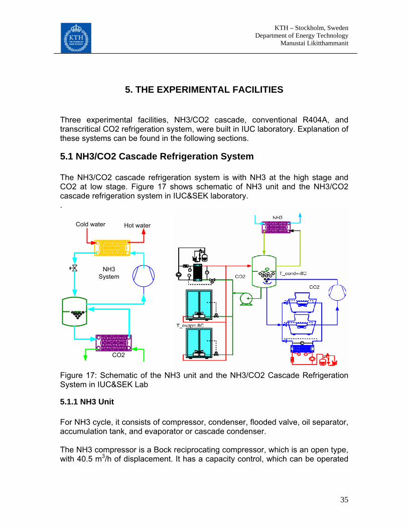
5.1 NH3/CO2 Cascade Refrigeration System The NH3/CO2 cascade refrigeration system is with NH3 at the high stage and CO2 at low stage. Figure 17 shows schematic of NH3 unit and the NH3/CO2 cascade refrigeration system in IUC&SEK laboratory. .
gure 17: Schematic of the NH3 unit and the NH3/CO2 Cascade Refrigeration
5.1.1 NH3 Unit
or NH3 cycle, it consists of compressor, condenser, flooded valve, oil separator,
he NH3 compressor is a Bock reciprocating compressor, which is an open type,
NH3System
Cold water Hot water
CO2
FiSystem in IUC&SEK Lab
Faccumulation tank, and evaporator or cascade condenser. Twith 40.5 m3/h of displacement. It has a capacity control, which can be operated

KTH – Stockholm, Sweden Department of Energy Technology Manustai Likitthammanit
36
both full load and half load. It has a 25 bar of maximum pressure and 700-1450 rpm of permissible range of rotation speeds.
Figure 18: Picture of NH3 Bock Reciprocating Compressor The cascade condenser is a plate heat exchanger that is specially selected to handle the pressure difference that will exist between CO2 and NH3, which is around 28 bars for CO2 at -8˚C and about 2.7 bars for NH3 at -12˚C.
Figure 19: Picture of Cascade Condenser Heat Exchanger Installed in the Facility
5.1.2 CO2 system The CO2 cycle consists of a compressor, accumulation tank, safety device, pump, oil separator, 2 freezing cabinets, 2 cooling cabinets, and 2 simulators. The CO2 compressor is a Copeland scroll compressor which can be operated between around -37 ˚C and -8 ˚C of temperature and 4.1 m3/h of displacement. It also has slight glass used to show oil level inside CO2 compressor. Figure 20 presents the picture of CO2 compressor.

KTH – Stockholm, Sweden Department of Energy Technology Manustai Likitthammanit
37
Slight Glass
Figure 20: Picture of CO2 Compressor
The accumulation tank has a capacity to contain 180 liters of CO2 which was installed with an electronic level indicator. It can stand a pressure of up to 40 bars or 6˚C. For protection from over pressure in the tank, the safety device was installed. The safety valve opens when the pressure reaches 38 bars. However, the opening of safety device can be avoided, which protects loss of CO2 refrigerant by using of a bleed valve, which will be opened when the pressure reaches 35 bars.
Figure 21: Picture of CO2 Accumulation Tank
KTH – Stockholm, Sweden Department of Energy Technology Manustai Likitthammanit
38
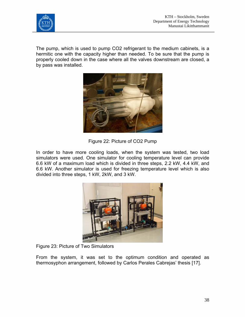
The pump, which is used to pump CO2 refrigerant to the medium cabinets, is a hermitic one with the capacity higher than needed. To be sure that the pump is properly cooled down in the case where all the valves downstream are closed, a by pass was installed.
Figure 22: Picture of CO2 Pump In order to have more cooling loads, when the system was tested, two load simulators were used. One simulator for cooling temperature level can provide 6.6 kW of a maximum load which is divided in three steps, 2.2 kW, 4.4 kW, and 6.6 kW. Another simulator is used for freezing temperature level which is also divided into three steps, 1 kW, 2kW, and 3 kW. Figure 23: Picture of Two Simulators From the system, it was set to the optimum condition and operated as thermosyphon arrangement, followed by Carlos Perales Cabrejas’ thesis [17].

KTH – Stockholm, Sweden Department of Energy Technology Manustai Likitthammanit
39
5.2 R404A Refrigeration System R404A refrigeration system is operated with R404A directly for freezing cabinets and indirectly for medium temperature cabinets. It has been designed and built in a separate project which investigates conventional refrigeration system. This system solution was chosen based on surveys among main companies in this field. This kind of system was commonly used in medium and large Swedish supermarkets, which could give a small charge in medium temperature circuit. For its system, it is quite different than NH3/CO2 cascade refrigeration system. Figure 24 represent schematic diagram of R404A refrigeration system.
Figure 24: Schematic Diagram of R404A Refrigeration System Both in Medium Temperature Level (left) and Freezing Temperature (right)
5.2.1 The Overall System of R404A Refrigeration System The R404 system can be divided into three parts where chillers No.1 and No.2 are used for cooling cabinets, and the third is use for freezing cabinets. In this system, R404A is used for both freezing and cooling cabinets. However, for cooling cabinets indirect system with Propylene glycol is used. In operation of the medium temperature circuit, brine goes through the chiller No. 2 to exchange heat with the primary refrigerant (R404A) in the evaporator. When it needs more cooling capacity, the electronic valve at chiller No.1 will open and then brine will go through the evaporator to exchange heat with R404A. This means compressor No.1 helps No.2 in providing the required cooling capacity when the load increases. After the brine exchanges heat with R404A in the evaporators, it will mix before flowing into the cabinets; this may result in some losses because

KTH – Stockholm, Sweden Department of Energy Technology Manustai Likitthammanit
40
of the different temperature. On the other hand, refrigerant R404A in the system rejects the condensers heat to a water loop. The freezers chiller No.3 is a direct expansion system. When the Bizter compressor operates, the refrigerant (R404A) is compressed with compressor and then exchanges heat with water in the condenser. After that, the refrigerant is reduced its pressure by expansion valve and then it goes though a freezing simulator and two freezing cabinets.
5.2.2 Components As can be seen in Figure 24, the R404A refrigeration system consists of three separate circuits: two are used for medium temperature cabinets and the other is used for freezers. Simulators are used when the system needs more loads. One simulator for cooling temperature level can provide 6 kW of a maximum load which is divided in three steps, 2 kW, 4 kW, and 6 kW. Another simulator is used for freezing temperature level which is also divided into three steps, 1.5 kW, 3 kW, and 4.5 kW. Moreover, for freezing temperature level, there is another simulator load, which is 2 kW. Thus the total load, which can provide for freezing cabinets, is 6.5 kW.
2 kW load
Figure 25: Two Simulators both for Freezer and Medium Temperature Level, and another Load for Freezer For medium temperature cabinets, two identical compressors are used. They are Copeland scroll type compressor. They have 20.9 m3/h of swept volume at 50 Hz of frequency and 32 bar of maximum pressure. They are connected with oil
KTH – Stockholm, Sweden Department of Energy Technology Manustai Likitthammanit
41
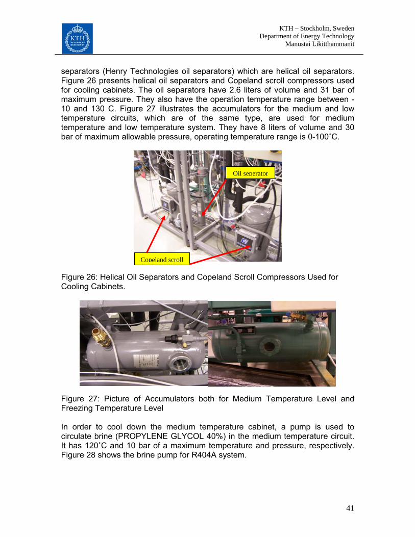
separators (Henry Technologies oil separators) which are helical oil separators. Figure 26 presents helical oil separators and Copeland scroll compressors used for cooling cabinets. The oil separators have 2.6 liters of volume and 31 bar of maximum pressure. They also have the operation temperature range between -10 and 130 C. Figure 27 illustrates the accumulators for the medium and low temperature circuits, which are of the same type, are used for medium temperature and low temperature system. They have 8 liters of volume and 30 bar of maximum allowable pressure, operating temperature range is 0-100˚C. Oil seperator
Copeland scroll
Figure 26: Helical Oil Separators and Copeland Scroll Compressors Used for Cooling Cabinets. Figure 27: Picture of Accumulators both for Medium Temperature Level and Freezing Temperature Level In order to cool down the medium temperature cabinet, a pump is used to circulate brine (PROPYLENE GLYCOL 40%) in the medium temperature circuit. It has 120˚C and 10 bar of a maximum temperature and pressure, respectively. Figure 28 shows the brine pump for R404A system.

KTH – Stockholm, Sweden Department of Energy Technology Manustai Likitthammanit
42
Figure 28: The Brine Pump For freezing cabinet, a semi-hermetic reciprocating Bizter compressor has 63.5 m3/ h of swept volume at 50 Hz of frequency. Maximum high pressure is 28 bars. It is connected with oil separator (ALCO Controls oil separators), which has 2.76 liters of volume and 31 bar of maximum pressure. They also have the operating temperature range between -10 and 150 C. Moreover, the accumulators, as shown in Figure 27, have 18 liters of volume and 43.1 bar of maximum allowable pressure, they can be operated between -18 and 120˚C. Figure 29 represents the picture of Bizter compressor and ALCO Controls oil separators. Figure 29: Picture of Bizter Compressor Used in Freezing Cabinets and ALCO Controls Oil Separators
KTH – Stockholm, Sweden Department of Energy Technology Manustai Likitthammanit
43
5.3 Transcritical CO2 Refrigeration System
5.3.1 The Overall System of Transcritical CO2 system Due to the temperature different in cascade condenser of NH3/CO2 cascade system, which can decrease COP of the system, the use of CO2 in both high and low stages can solve this problem. The use of CO2 both high and low stages will avoid the usage of cascade condenser. Without cascade condenser, however, oil separator has to work well to collect oil not to accumulate in the tank. Therefore, in this experiment, the system was tested without sub system. The evaporator was installed instead of the tank to avoid potential oil problems. Figure 30 shows schematic diagram of transcritical CO2 refrigeration system, which consists of 2-stage compressor, intermediate heat exchanger, oil separator, internal heat exchanger, expansion valve, cascade condenser, and accumulator. For the working of transcritical CO2 system, evaporator is used to exchanger heat with brine controlled its temperature by shut control as described above. Then only liquid of CO2 refrigerant will flows to accumulate in accumulation, which is used to separate between liquid and vapour of CO2. Only CO2 vapour from accumulator will go out and exchange heat with CO2 from gas cooler to get some superheat which can avoid liquid go to the compressor. After that CO2 vapour will be compressed by CO2 compressor at first stage before it goes though the intermediate heat exchanger to exchange heat with water supply from IUC&SEK laboratory. The outlet water temperature of intermediate heat exchanger can be controlled by adjusting of water flow rate at the inlet of intermediate heat exchanger. Before CO2 refrigerant goes though the gas cooler, it is compressed by CO2 compressor at second stage and then it is separated oil with oil separator. While CO2 vapour goes to the gas cooler, separated oil is accumulated in the bottom of oil separator. When the level of oil is too low, the automatic valve will open and the oil will be sucked back to the compressor. After the CO2 goes out from gas cooler, temperature of CO2 will decrease by passing the internal heat exchanger which helps to increase cooling capacity. Finally, pressure of CO2 will be reduced by expansion valve before go back to evaporator. Figure 31 presents the picture of transcritical CO2 system.

KTH – Stockholm, Sweden Department of Energy Technology Manustai Likitthammanit
44
27 kW
Water
Water
5 kW
7 kW
4 kW
29 kW
9 kW
Transcritical CO2 systemGas Cooler
Oil Seperator
Compressor stage 2
Intermediate HEX
Compressor stage 1
Internal HEX
Accumulator
Evaporator
Brin Figure 30: Schematic Diagram of the Transcritical CO2 System
Figure 31: Picture of Transcritical CO2 system

KTH – Stockholm, Sweden Department of Energy Technology Manustai Likitthammanit
45
5.3.2 Two-Stage Compressor Two-stage compressor operates with 7 and 4 kW of input power in the first and second stage, respectively. It is a Dorin semi-hermetic compressor which has 2900 rpm of compressor speed and 10.3 m3/h of swept volume [18]. Furthermore, this compressor has been designed to resist pressure of 100 bar in suction and 163 bar in discharge with two safety relief valves. The maximum tolerated pressure difference is 90 bar. The maximum allowable temperature at the high pressure is 180˚C. It operates with on-off control. Figure 32 shows the picture of the two-stage CO2 compressor.
Discharge 2nd
Discharge 1st stage Suction 2nd stage
Suction 1st
Figure 32: Picture of the Two-Stage CO2 Compressor
5.3.3 Heat Exchangers The gas cooler, evaporator, and intermediate heat exchanger are the Supermax TM all welded plate heat exchanger which incorporates the benefits of plate and frame exchangers without gaskets [22], they are counter-flow heat exchanger. The gas cooler, as shown in Figure 33, has 29 kW of capacity and 48 plates. It can operate under 130 bar of the maximum tested pressure and 100˚C of the maximum designed temperature. In addition, there are 6.07 and 4.08 liters of volume for CO2 and water, respectively.

KTH – Stockholm, Sweden Department of Energy Technology Manustai Likitthammanit
46
CO2 inlet
CO2 Water
Water outlet
Figure 33: Picture of the Gas Cooler Figure 34 presents the evaporator (cascade condenser) which has a capacity of 27 kW the number of plates is 80. It can operate with 91bar of a maximum designed pressure and 50˚C of a maximum designed temperature. The evaporator has 10.37 and 6.97 liters of volume for CO2 and water, respectively.
Figure 34: Picture of the Evaporator (Cascade Condenser) To reduce the discharge temperature and input power to the system, an intermediate heat exchanger is used to reject heat between the compressor stages. The intermediate heat exchanger has 26 plates and a capacity of 9 kW. It can with stand similar conditions as the evaporator, and has 3.54 and 2.38 liters of volume for CO2 and water, respectively. Figure 35 shows the picture of intermediate heat exchanger.
CO2 outlet Water inlet
CO2 inlet
Water outlet

KTH – Stockholm, Sweden Department of Energy Technology Manustai Likitthammanit
47
From gas cooler
To comp
From Accumulator
To expansion valve
Figure 35: Picture of Intermediate Heat Exchanger
CO2 inlet
Water outlet
Water inlet
CO2 outlet
For the internal heat exchanger, as presented in Figure 36, which can stand pressure up to 200 bar, it is different with other heat exchangers as it is a shell and tube heat exchanger with around 5 kW of capacity. The heat is exchanged between CO2 from gas cooler, which has 0.064 liters of volume, and CO2 from accumulator, which has 0.3 liters of volume. Figure 36: Picture of Internal Heat Exchanger 5.3.4 Accumulator Accumulator, which can stand pressure up to 200 bar and has a volume of around 3.013 liters, is located between cascade condenser and inter cooler which is used to separate vapor from the liquid of CO2 refrigerant before vapor of

KTH – Stockholm, Sweden Department of Energy Technology Manustai Likitthammanit
48
carbon dioxide refrigerant goes through the inter cooler and then to two stage compressor. It is designed by Jörgen Rogstam and Per-Olof Nilsson at IUC&SEK (Installatörernas Utbildningscentrum and Sveriges Energi & Kylcentrum). The reference of Its design is the accumulator for automotive air conditioning system [23]. However, the accumulator used in automotive air conditioning is used R134a as refrigerant. While the accumulator is in operation, CO2 refrigerant flows from the cascade condenser into the accumulator, vapor will be separated from the liquid and sucked out by the compressor, liquid CO2 will remain at the bottom of the accumulator. Error! Reference source not found. presents the pictures of the accumulator opened and closed. Any oil flowing in the system, after the oil separator will be dissolved in the accumulator liquid. Therefore, a 1mm hole is made in the suction line to return some of the oil to the compressor, the hole in the suction line can be seen in Figure 38.
CO2 vapor
CO2 liquid and vapor inlet
Figure 37: Picture of Inside of Accumulator (left) and Accumulator (right)
Small hole for releasing oil Figure 38: Picture of Small Hole for Releasing Oil from CO2 Refrigerant
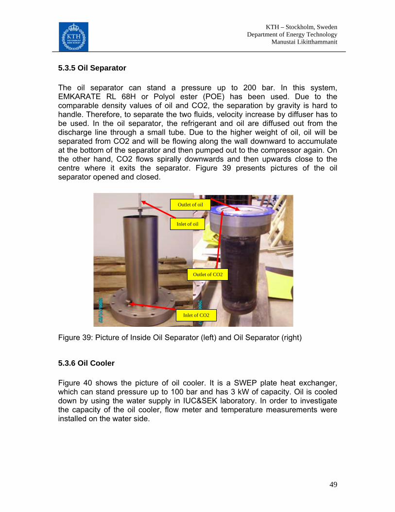
KTH – Stockholm, Sweden Department of Energy Technology Manustai Likitthammanit
49
5.3.5 Oil Separator The oil separator can stand a pressure up to 200 bar. In this system, EMKARATE RL 68H or Polyol ester (POE) has been used. Due to the comparable density values of oil and CO2, the separation by gravity is hard to handle. Therefore, to separate the two fluids, velocity increase by diffuser has to be used. In the oil separator, the refrigerant and oil are diffused out from the discharge line through a small tube. Due to the higher weight of oil, oil will be separated from CO2 and will be flowing along the wall downward to accumulate at the bottom of the separator and then pumped out to the compressor again. On the other hand, CO2 flows spirally downwards and then upwards close to the centre where it exits the separator. Figure 39 presents pictures of the oil separator opened and closed.
Inlet of CO2
Outlet of CO2
Outlet of oil
Inlet of oil
Figure 39: Picture of Inside Oil Separator (left) and Oil Separator (right)
5.3.6 Oil Cooler Figure 40 shows the picture of oil cooler. It is a SWEP plate heat exchanger, which can stand pressure up to 100 bar and has 3 kW of capacity. Oil is cooled down by using the water supply in IUC&SEK laboratory. In order to investigate the capacity of the oil cooler, flow meter and temperature measurements were installed on the water side.

KTH – Stockholm, Sweden Department of Energy Technology Manustai Likitthammanit
50
Figure 40: Picture of Oil Cooler
5.3.7 Expansion Valve The expansion valve is a Danfoss electronic valve. It consists of two parts: one is the controller (ICAD 60DS) and the other is the valve (ICMT). For ICAD 600S, it can be set with on off digital input and it can operate in the temperature range between -30˚C and 50˚C. It has 140 bar of maximum working pressure and can be operated with volume flow rate range between 0.6-4.6 m3/h. Error! Reference source not found. shows picture of the expansion valve.
Figure 41: Picture of Expansion Valve
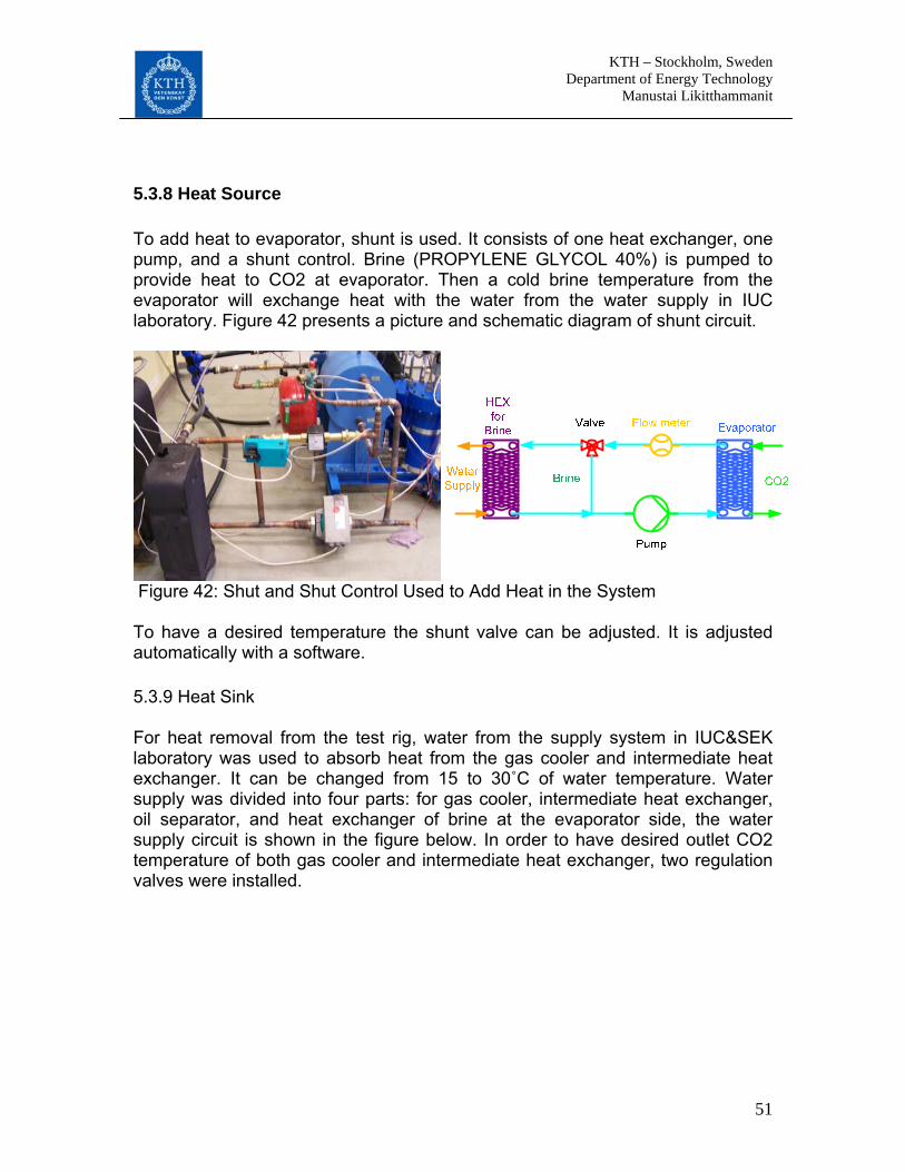
KTH – Stockholm, Sweden Department of Energy Technology Manustai Likitthammanit
51
5.3.8 Heat Source To add heat to evaporator, shunt is used. It consists of one heat exchanger, one pump, and a shunt control. Brine (PROPYLENE GLYCOL 40%) is pumped to provide heat to CO2 at evaporator. Then a cold brine temperature from the evaporator will exchange heat with the water from the water supply in IUC laboratory. Figure 42 presents a picture and schematic diagram of shunt circuit.
Figure 42: Shut and Shut Control Used to Add Heat in the System To have a desired temperature the shunt valve can be adjusted. It is adjusted automatically with a software. 5.3.9 Heat Sink For heat removal from the test rig, water from the supply system in IUC&SEK laboratory was used to absorb heat from the gas cooler and intermediate heat exchanger. It can be changed from 15 to 30˚C of water temperature. Water supply was divided into four parts: for gas cooler, intermediate heat exchanger, oil separator, and heat exchanger of brine at the evaporator side, the water supply circuit is shown in the figure below. In order to have desired outlet CO2 temperature of both gas cooler and intermediate heat exchanger, two regulation valves were installed.

KTH – Stockholm, Sweden Department of Energy Technology Manustai Likitthammanit
52
Figure 43: Water Supply for Gas Cooler and Intermediate Heat Exchanger
5.3.10 Pipes and Tube Dimension The piping system can be divided into two parts: one for the CO2 cycle and the other for water, which is used to cool down the refrigerant in heat exchangers. For primary CO2 cycle, all of pipes are stainless steel pipes, which have two diameters (16 mm and 12 mm). Table 3 shows the primary circuit piping and the corresponding internal diameters. Table 3: The Primary Refrigeration Piping Consist the Following Insider Tube Diameter
Tube Suction Tube Length (cm) Tube inside diameter (mm) Suction line 37 16 Comp 1st stage and Internal Ex 82 12 Internal Ex and Comp 2nd stage 18.5 12 Comp 2nd stage and Oil separator 113 12 Discharge line 132 12 Gas cooler and inter cooler 90.5 12 Liquid line 75 12 Cascade condenser and Accumulator 63 12 Accumulator and Inter cooler 15 16
5.3.11 The Measurement and Controller Facilities The measurement devices consist of the main part listed below:
• Agilent data acquisition device • Shunt control (Inlet water temperature control in evaporator)

KTH – Stockholm, Sweden Department of Energy Technology Manustai Likitthammanit
53
• Expansion valve control • Oil level control • 2 flow turbine type meters • Power meter • Others (pressure gages, light alarms, and on-off switch control)
At the first step of testing the system running in short periods, 21 thermocouples and 10 pressure transducers have been connected to various points in the system both in CO2 and water sides. Below is a list of the measuring points.
5.3.10.1 Positions of Pressure Transducers
1. At CO2 inlet of stage 1st compressor (P_Comp1_In) 2. At CO2 outlet of stage 1st compressor (P_Comp1_Out) 3. At CO2 inlet of stage 2nd compressor (P_Comp2_In) 4. At CO2 outlet of stage 2nd compressor (P_Comp2_Out) 5. At CO2 inlet of gas cooler (P_Gascooler_In) 6. At CO2 outlet of gas cooler (P_Gascooler_out) 7. At CO2 inlet of expansion valve (P_ExpanV_In) 8. At CO2 inlet of evaporator (P_Evap_In) 9. At CO2 outlet of evaporator (P_Evap_Out) 10. At CO2 outlet of accumulator (P_Accum_Out)
5.3.10.2 Positions of Thermocouples
1. At CO2 inlet of stage 1st compressor (T_Comp1_In) 2. At CO2 outlet of stage 1st compressor (T_Comp1_Out) 3. At water inlet of intermediate heat exchanger (T_W_MHEX_In) 4. At water outlet of intermediate heat exchanger (T_W_MHEX_Out) 5. At CO2 inlet of stage 2nd compressor (T_Comp2_In) 6. At CO2 outlet of stage 2nd compressor (T_Comp2_Out) 7. Before oil return valve (T_Oil_Return_Bef) 8. After oil return valve (T_Oil_Return_Af) 9. At oil inlet of oil cooler (T_Oil_HEX_In) 10. At oil outlet of oil cooler (T_Oil_HEX_Out) 11. At water outlet of oil cooler (T_W_OilCooler_Out) 12. At CO2 inlet of gas cooler (T_Gascooler_In) 13. At CO2 outlet of gas cooler (T_Gascooler_Out) 14. At water outlet of gas cooler(T_W_Gascooler_Out) 15. At CO2 inlet of expansion valve (T_ExpanV_In) 16. At water inlet of evaporator (T_W_Evap_In) 17. At water outlet of evaporator (T_W_Evap_Out) 18. At CO2 outlet of evaporator (T_Evap_Out) 19. At CO2 outlet of accumulator (T_Accum_Out)

KTH – Stockholm, Sweden Department of Energy Technology Manustai Likitthammanit
54
20. At water outlet of water supply (T_W_Supply_Out) To measure water flow rate, two turbine type flow meters were installed at brine side of the evaporator and water side of the oil cooler. All thermocouples, pressure transducers, flow meter, and power meter were connected though Agilent data acquisition device where it was possible to track the system trends on computer. To collect data to the computer, Agilent VEE Pro software, was used. For controlling software, there are 3 main parts. First is to control evaporating pressure. According to Figure 8, COP of transcritical system is influenced by varying high side pressure; this investigation needs to have a constant evaporating pressure. The software reads the evaporating pressure from pressure transducer in voltage (V) and converts it to the pressure, following the relation that 1 to 5 voltages corresponds 1 to 150 bar (absolute pressure) as can be seen in equation [3-12]. Then the evaporating pressure signal is fed to PID controller to regulate the shunt valve. Second is to control heat source. In this case, the inlet water temperature of evaporator is used as the reference. It is measured by a thermocouple and is fed into PID controller. Then it is also sent to control the shunt valve. Final is to control the expansion valve. The expansion valve is controlled in order to get the optimum COP, outlet CO2 temperature of the gas cooler is used as the reference. When it is read, it is converted to optimum pressure before it is sent in to PID control. The equation below is used to relate the gas cooler outlet temperature to the optimum discharge pressure, it is a curve fit of the optimum discharge pressure at different gas cooler exist temperatures. Figure 44 illustrates the diagrams of three controllers.
1.6)__*7.2( −= OutGascoolerTPopt (1)

KTH – Stockholm, Sweden Department of Energy Technology Manustai Likitthammanit
55
Figure 44: Diagram for Evaporating Pressure Control (left), Expansion Valve Control (middle) and for Shut Control (right) To demonstrate the important values on a computer screen during testing, all data are collected in term array through Agilent data acquisition device and then they were separated into 3 main parts: temperature, pressure, and electric power consumption, as can be seen in Figure 45. For pressures, voltage signals (V) from different pressure transducers were collected and converted into different pressures.
25.37)*25.37(551035.01_1_ −++= VInCompP (2)
25.37)*25.37(319720.01_1_ −++= VOutCompP (3)
25.37)*25.37(481674.01_2_ −+−= VinCompP (4)
25.37)*25.37(591114.01_2_ −+−= VOutCompP (5)
25.37)*25.37(604454.01__ −+−= VInGascoolerP (6)
25.37)*25.37(806211.11__ −++= VOutGascoolerP (7) 25.37)*25.37(400914.01__ −+−= VInExpanVP (8)
25.37)*25.37(379503.01__ −+−= VInEvapP (9)

KTH – Stockholm, Sweden Department of Energy Technology Manustai Likitthammanit
56
25.37)*25.37(525316.01__ −+−= VOutEvapP (10)
25.37)*25.37(306009.01__ −++= VOutAccumP (11)
For temperatures, all temperatures were read in °C, which are directly displayed in computer screen. For electric power consumption, pulses from power meters are collected and convert to kW. Furthermore, there were some more important values, such as optimum discharged pressure, optimum intermediate pressure, superheat in the evaporator, accumulator, and before the compressor. For the optimum discharged pressure, it could be seen in equation [1] above, while for the optimum intermediate pressure, it can be related to the CO2 outlet temperature of the intermediate heat exchanger, the following correlation which is a curve fit of the optimum intermediate pressure can be used as a guideline. In order to avoid CO2 liquid flowing into the compressor, the superheat value was displayed on the computer screen. If no superheat, for example, CO2 compressor must be stopped. On the computer screen, optimum discharge and intermediate pressures were also shown to give an idea of how the system is running and perform the proper adjustments. The figure below shows how the data values are displayed on the computer screen.
Figure 45: The Display of Data on Computer Screen

KTH – Stockholm, Sweden Department of Energy Technology Manustai Likitthammanit
57
For the proper control of oil level, a regulation valve was installed on the oil return line. When the oil level is too low, the valve is opened manually to return the oil in the separator back to the compressor. The oil in the compressor also had temperature control which has a range between 30 and 65˚C.
5.3.12 Safety Device To know if oil pressure (90 bar) and thermistors (temperature sensor of an electric motor in CO2 compressor, respectively, reach dangerous levels, light alarms are installed. Figure 46 presents pictures of thermistors and oil pressure alarm.
Figure 46: Pictures of Thermistors and Oil Pressure Alarm. Safety valves in the compressor were calibrated at 158 bar for high pressure and at 97 bar for low pressure. Electro-mechanical pressure switch was also installed. It was set at 110 bar of a maximum permissible pressure at discharge pressure. Furthermore, two relief valves which were calibrated at 130 bar for high pressure and 80 bar for low pressure. They were also installed to release CO2 from the system when the CO2 pressure is too high. Figure 47 presents the picture of electromechanical pressure and relief valve.

KTH – Stockholm, Sweden Department of Energy Technology Manustai Likitthammanit
58
Figure 47: Pictures of Electromechanical Pressure and Relief Valve
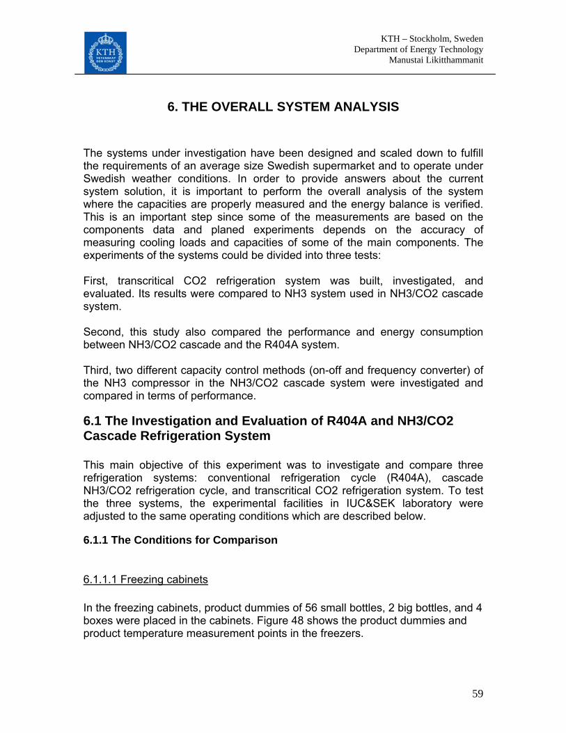
KTH – Stockholm, Sweden Department of Energy Technology Manustai Likitthammanit
59
6. THE OVERALL SYSTEM ANALYSIS The systems under investigation have been designed and scaled down to fulfill the requirements of an average size Swedish supermarket and to operate under Swedish weather conditions. In order to provide answers about the current system solution, it is important to perform the overall analysis of the system where the capacities are properly measured and the energy balance is verified. This is an important step since some of the measurements are based on the components data and planed experiments depends on the accuracy of measuring cooling loads and capacities of some of the main components. The experiments of the systems could be divided into three tests: First, transcritical CO2 refrigeration system was built, investigated, and evaluated. Its results were compared to NH3 system used in NH3/CO2 cascade system. Second, this study also compared the performance and energy consumption between NH3/CO2 cascade and the R404A system. Third, two different capacity control methods (on-off and frequency converter) of the NH3 compressor in the NH3/CO2 cascade system were investigated and compared in terms of performance.
6.1 The Investigation and Evaluation of R404A and NH3/CO2 Cascade Refrigeration System This main objective of this experiment was to investigate and compare three refrigeration systems: conventional refrigeration cycle (R404A), cascade NH3/CO2 refrigeration cycle, and transcritical CO2 refrigeration system. To test the three systems, the experimental facilities in IUC&SEK laboratory were adjusted to the same operating conditions which are described below.
6.1.1 The Conditions for Comparison
6.1.1.1 Freezing cabinets In the freezing cabinets, product dummies of 56 small bottles, 2 big bottles, and 4 boxes were placed in the cabinets. Figure 48 shows the product dummies and product temperature measurement points in the freezers.
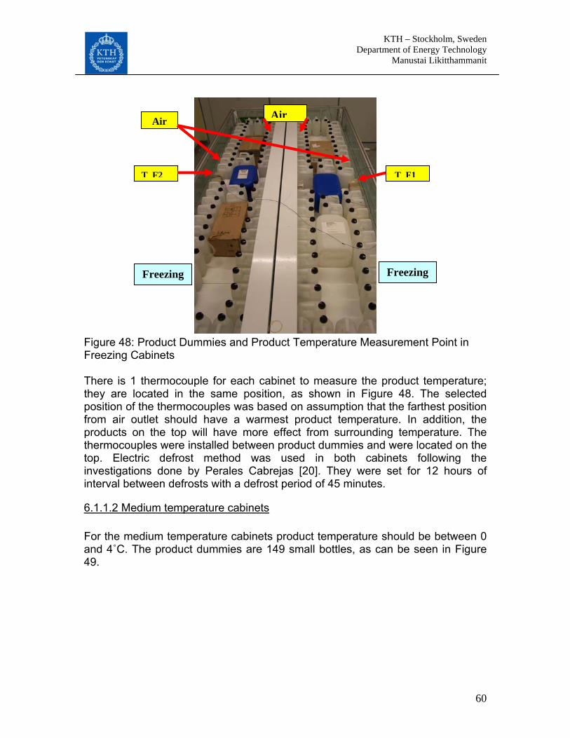
KTH – Stockholm, Sweden Department of Energy Technology Manustai Likitthammanit
60
Freezing Freezing
T F2 T F1
Air Air Figure 48: Product Dummies and Product Temperature Measurement Point in Freezing Cabinets There is 1 thermocouple for each cabinet to measure the product temperature; they are located in the same position, as shown in Figure 48. The selected position of the thermocouples was based on assumption that the farthest position from air outlet should have a warmest product temperature. In addition, the products on the top will have more effect from surrounding temperature. The thermocouples were installed between product dummies and were located on the top. Electric defrost method was used in both cabinets following the investigations done by Perales Cabrejas [20]. They were set for 12 hours of interval between defrosts with a defrost period of 45 minutes.
6.1.1.2 Medium temperature cabinets For the medium temperature cabinets product temperature should be between 0 and 4˚C. The product dummies are 149 small bottles, as can be seen in Figure 49.
KTH – Stockholm, Sweden Department of Energy Technology Manustai Likitthammanit
61
T M2 ProductT_M2_AirIn
T_M2_AirOut
Figure 49: Product Dummies and Product Temperature Measurement Point in Cooling Cabinet 2 as the Example. Temperature measurements where done in similar way as done in the freezers. Positions of the thermocouples are shown in Figure 49. The selected positions of the thermocouples were based on the investigations done by Perales Cabrejas [17]. For the defrost parameters of cooling cabinets, refrigeration was stopped for a certain period in order to melt the frost using the heat of the surrounding air. They were set for 24 hours of interval between defrosts and 45 minutes for each defrost period.
6.1.1.3 Air Temperature and relative humidity in the IUC&SEK lab Air temperature in the laboratory influences the cooling capacity of the cabinets. So it was kept almost constant and around 20˚C.Error! Reference source not found. Figure 50 shows air temperature in the laboratory.

KTH – Stockholm, Sweden Department of Energy Technology Manustai Likitthammanit
62
Figure 50: Air Temperature in the Laboratory Set around 20 ˚C High humidity will also increase the cooling load in the cabinets due to condensation of water and frost forming on the evaporator, cabinets and the products. Figure 51 presents Psychometric chart, which shows the higher humidity, the higher enthalpy.
Figure 51: Psychometric Chart, which presents the higher humidity, the higher enthalpy.

KTH – Stockholm, Sweden Department of Energy Technology Manustai Likitthammanit
63
Figure 52: The Relative Humidity in the Lab
6.1.2 NH3/CO2 Cascade Refrigeration System The ammonia compressor was used to determine the mass flow rate of the refrigerant which would then be used to calculate the cooling capacity of the ammonia system. The swept volume of the compressor is known from the manufacturer data. Measuring the rotational speed of the compressor, temperatures and pressures around it gave all the data needed to calculate the mass flow of the refrigerant. According to Perales Cabrejas [17], the volumetric efficiency which was used in the mass flow calculations of ammonia cycle, had to be adjusted. The formula could be expressed below:
)063.0exp(094.1,inlet
outletadjustedV P
P⋅−⋅=η (12)
To calculate mass flow of ammonia cycle, the volumetric efficiency, the density at suction line, and swept volume flow were need:
(13) insNH Vm ρη ⋅⋅= && v3
The compressor had a displacement of 40.5 msrV 3/ h in full capacity mode and 20.25 m3/ h for reduced capacity (half capacity) mode both at rated speed of 1450 rpm. Swept volume flow in m
rn3/s at a given speed could then be calculated
using the relation:
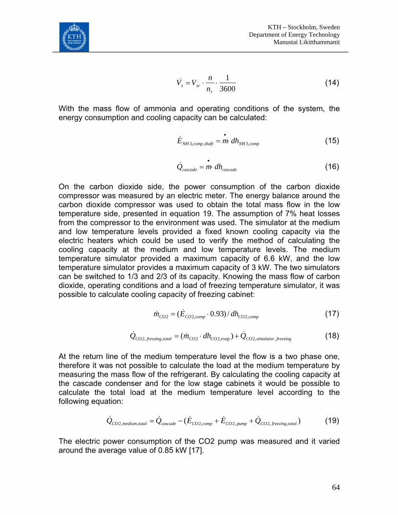
KTH – Stockholm, Sweden Department of Energy Technology Manustai Likitthammanit
64
36001
⋅⋅=r
srs nnVV& (14)
With the mass flow of ammonia and operating conditions of the system, the energy consumption and cooling capacity can be calculated:
compNHshaftcompNH dhmE ,3,,3 ⋅=•
& (15)
cascadecascade dhmQ ⋅=•
& (16)
On the carbon dioxide side, the power consumption of the carbon dioxide compressor was measured by an electric meter. The energy balance around the carbon dioxide compressor was used to obtain the total mass flow in the low temperature side, presented in equation 19. The assumption of 7% heat losses from the compressor to the environment was used. The simulator at the medium and low temperature levels provided a fixed known cooling capacity via the electric heaters which could be used to verify the method of calculating the cooling capacity at the medium and low temperature levels. The medium temperature simulator provided a maximum capacity of 6.6 kW, and the low temperature simulator provides a maximum capacity of 3 kW. The two simulators can be switched to 1/3 and 2/3 of its capacity. Knowing the mass flow of carbon dioxide, operating conditions and a load of freezing temperature simulator, it was possible to calculate cooling capacity of freezing cabinet:
compCOcompCOCO dhEm ,2,22 /)93.0( ⋅= && (17)
freezingsimulatorCOevapCOCOtotalfreezingCO QdhmQ ,,2,22,,2 )( &&& +⋅= (18)
At the return line of the medium temperature level the flow is a two phase one, therefore it was not possible to calculate the load at the medium temperature by measuring the mass flow of the refrigerant. By calculating the cooling capacity at the cascade condenser and for the low stage cabinets it would be possible to calculate the total load at the medium temperature level according to the following equation:
)( ,,2,2,2,,2 totalfreezingCOpumpCOcompCOcascadetotalmediumCO QEEQQ &&&&& ++−= (19) The electric power consumption of the CO2 pump was measured and it varied around the average value of 0.85 kW [17].
KTH – Stockholm, Sweden Department of Energy Technology Manustai Likitthammanit
65
The coefficient of performance (COP) was used to evaluate the performance of the system and it was also used for comparisons between the different systems. To evaluate different cascade system sections, four COPs can be defined. First, for the ammonia system, the COP could be evaluated by knowing the cooling capacity at cascade condenser and the total energy consumption of ammonia compressor, which could express as this formula:
compNHcascadeNH EQCOP ,33 / &&= (21) Second, for COP for the low temperature level, the COP was evaluated using the useful refrigerating capacities from low temperature level divided by the total energy consumption used to cool the products only in freezing cabinets. In order to calculate energy consumption used to cool down the products in freezing cabinets, the COP of ammonia system and the cooling capacity of low temperature level were used according to the following relations:
3,2,,2,3 /)( NHcompCOtotalfreezingCOfreezingNH COPEQE &&& += (22)
compCOfreezingNHtotalfreezingCO EEE ,2,3,,2&&& += (23)
totalfreezingCOtotalfreezingCOtotalfreezngCO EQCOP ,,2,,2,,2 / &&= (24)
Third, for the system of medium temperature level, the COP was evaluated in the same way as the COP of low temperature level, the used formulas are shown below:
3,2,,2,3 /)( NHpumpCOtotalmediumCOmediumNH COPEQE &&& += (25)
pumpCOmediumNHtotalmediumCO EEE ,2,3,,2&&& += (26)
totalmediumCOtotalmediumCOtotalmediumCO EQCOP ,,2,,2,,2 / &&= (27)
Final, the overall system COP was evaluated using the useful refrigerating capacities from both medium and low temperature levels divided by the sum of the carbon dioxide compressor and power consumption of pump plus the ammonia compressor as follows:
compNHcompCOpumpCO
totalfreezingCOtotalmediumCOTotalCONH EEE
QQCOP
,3,2,2
,,2,,2,2_3 &&&
&&
++
+= (28)
KTH – Stockholm, Sweden Department of Energy Technology Manustai Likitthammanit
66
6.1.3 R404A Refrigeration System The R404A system analysis was not much different from the cascade system. The system could be divided in two parts; the medium temperature and low temperature levels. The mass flow rate of R404A for both parts, shown in Figure 24, can be calculated by energy balance around each compressor in a similar way to the CO2 compressor in the cascade system, explained in the section above.
The simulators at both medium and low temperature levels can provide a fixed known cooling capacity via the electric heaters. The total cooling capacity of medium temperature level is then calculated as follows:
mediumsimsystemmediumARsystemmediumARtotalmediumAR QQQQ ,2,,4041,,404,,404 ++= (29) The energy consumption of the brine pump at the medium temperature level is calculated by measuring the current and voltage [equation 30]. This pump operated at variable speed; thus, to evaluate its energy consumption the average of the maximum and minimum energy consumptions was used:
IVE pumpbrine ⋅⋅= 3, (30)
Three different COPs of R404A system was defined: for low temperature level, for medium temperature level, and for the overall system. The COP of freezing temperature level is calculated by using the cooling capacity of low temperature level and the energy consumption of compressor No.3 in Figure 24:
3,404,,404,,404 / compARtotalfreezingARtotalfreezingAR EQCOP = (31)
In a similar was the COP of medium temperature level is calculated as:
(32) )/( ,2,4041,404,,404,,404 pumpbrinecompARcompARtotalmediumARtotalmediumAR EEEQCOP &++= The overall system COP is calculated using the useful refrigerating capacities from both medium and low temperature levels divided by the sum of the energy consumption of three compressors and the pump:
3,4042,4041,404,
,,,404
compARcompARcompARpumpbrine
totalfreezingtotalmediumTotalAR EEEE
QQCOP
+++
+=
&&&
&& (33)

KTH – Stockholm, Sweden Department of Energy Technology Manustai Likitthammanit
67
6.2 The investigation and evaluation of two different capacity control types (on-off and variable speed) of NH3 compressor in NH3/CO2 cascade refrigeration system Two different capacity control methods (on-off and variable frequency speed) of the NH3 compressor were investigated and compared in term of power consumption. The conditions in the laboratory were set in the same as pervious test both in air temperature and relative humidity. The period of each test is 4 hours. To avoid effect from defrost, it was turned off during the test. For the system analysis, between equation 12 and 16 for NH3/CO2 could be used.
6.3 The investigation and evaluation of transcritical CO2 refrigeration system The main objective of this experiment is to investigate and evaluate transcritical CO2 refrigeration system. For technical concerns and limited time frame, the transcritical CO2 system was investigated and evaluated separately without being connected to the low temperature circuit. The cooling capacity of the evaporator is calculated from the brine loop side, shown in Figure 42. With two thermocouples in brine inlet and outlet of evaporator, and flow meter at inlet of the brine side, the cooling capacity is calculated according to the following equation:
)*(* _______ OutEvapBInEvapBEvapBEvapBEvapB TTCpmQ −= && (34)
Electric power consumption of the compressor is measured and the system COP is calculated as follows:
eleEvapB EQCOP /_= (35) CO2 mass flow was calculated by performing energy balance around the CO2 compressor according to the diagram in Figure 53. As shown in equation 36, energy input, which consists of electric input power and input energy at suction line, has to be equal with energy output, which consists of capacity of oil cooler, energy loss to surrounding, capacity of intercooler, and output power at discharge line.

KTH – Stockholm, Sweden Department of Energy Technology Manustai Likitthammanit
68
Electric Input Power
Inlet Energy
Capacity of InMHEX
Capacity of Oil Cooler
Energy loss
outlet Energy
Figure 53: Diagram of Energy Balance around the two stage CO2 compressor
lossInMHEXOilCoolerOutndCompCOInstCompCOelec QQQhmhmE &&&&&& +++=+ )*()*( _22_12 (36)
Or
lossOilCoolerndCompCOstCompCOelec QQdhmdhmE &&&&& +++= )*()*( 2212
The capacity of the intercooler can be calculated by using the mass flow rate and conditions at the inlet and outlet of intercooler:
)(* _1__2_2 OutstCompInndCompCOInMHEW hhmQ −= && (37)
7% of energy loss in the compressor was assumed where:
100/*7 eleloss EQ && = (38) Knowing the CO2 mass flow, capacities in gas cooler and internal heat exchanger can be calculated as follows:
)(* __2 OutGascoolerInGascoolerCOgascooler hhmQ −= && (39)
)(* __2 InEvapOutGascoolerCOInHEX hhmQ −= && (40)
Input powers and isentropic efficiencies in CO2 compressor both in two stages were calculated according to:
KTH – Stockholm, Sweden Department of Energy Technology Manustai Likitthammanit
69
)(* _1_121 InstCompOutstCompCOst hhmE −= && (41)
)(* _2_222 InndCompOutndCompCOnd hhmE −= && (42)
)/()( _1__1__1__1_1 InstCompOutstCompInstCompisstCompst hhhh −−=η (43)
)/()( _2__2__2__2_2 InndCompOutndCompInndCompisndCompnd hhhh −−=η (44)
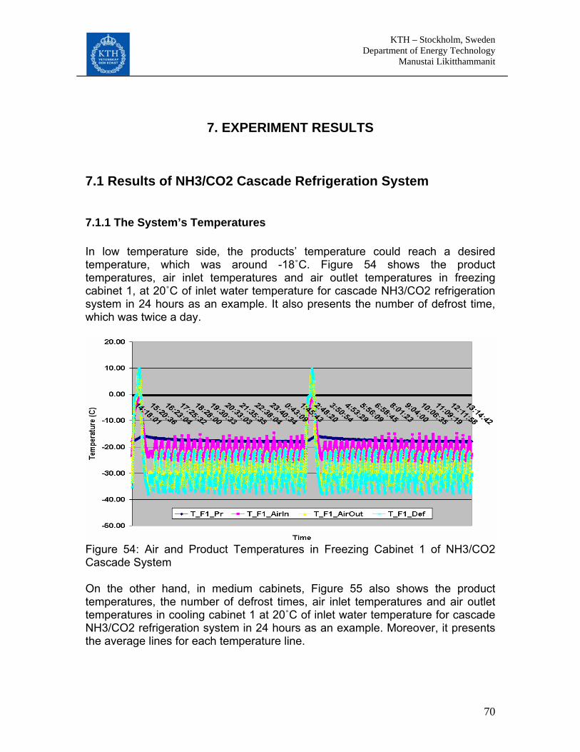
KTH – Stockholm, Sweden Department of Energy Technology Manustai Likitthammanit
70
7. EXPERIMENT RESULTS
7.1 Results of NH3/CO2 Cascade Refrigeration System
7.1.1 The System’s Temperatures In low temperature side, the products’ temperature could reach a desired temperature, which was around -18˚C. Figure 54 shows the product temperatures, air inlet temperatures and air outlet temperatures in freezing cabinet 1, at 20˚C of inlet water temperature for cascade NH3/CO2 refrigeration system in 24 hours as an example. It also presents the number of defrost time, which was twice a day.
Figure 54: Air and Product Temperatures in Freezing Cabinet 1 of NH3/CO2 Cascade System On the other hand, in medium cabinets, Figure 55 also shows the product temperatures, the number of defrost times, air inlet temperatures and air outlet temperatures in cooling cabinet 1 at 20˚C of inlet water temperature for cascade NH3/CO2 refrigeration system in 24 hours as an example. Moreover, it presents the average lines for each temperature line.
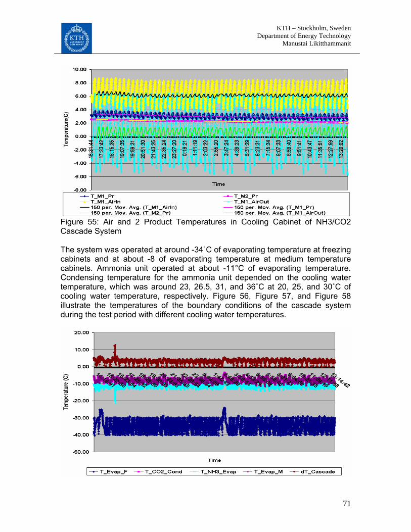
KTH – Stockholm, Sweden Department of Energy Technology Manustai Likitthammanit
71
Figure 55: Air and 2 Product Temperatures in Cooling Cabinet of NH3/CO2 Cascade System The system was operated at around -34˚C of evaporating temperature at freezing cabinets and at about -8 of evaporating temperature at medium temperature cabinets. Ammonia unit operated at about -11°C of evaporating temperature. Condensing temperature for the ammonia unit depended on the cooling water temperature, which was around 23, 26.5, 31, and 36˚C at 20, 25, and 30˚C of cooling water temperature, respectively. Figure 56, Figure 57, and Figure 58 illustrate the temperatures of the boundary conditions of the cascade system during the test period with different cooling water temperatures.

KTH – Stockholm, Sweden Department of Energy Technology Manustai Likitthammanit
72
Figure 56: Operating Temperatures of the NH3/CO2 Cascade System at 20˚C of Cooling Water Temperature.
Figure 57: Operating Temperatures of the NH3/CO2 Cascade System at 25˚C of Cooling Water Temperature
Figure 58: Temperatures of Boundary Conditions in the NH3/CO2 Cascade System at 30˚C of Cooling Water Temperature

KTH – Stockholm, Sweden Department of Energy Technology Manustai Likitthammanit
73
7.1.2 Cooling Capacity As explained earlier, the mass flow rate of CO2 refrigerant in CO2 cycle was calculated by measured power consumption and the 7% of loss in the compressor power. In NH3 system, its mass flow rate was calculated using manufacturer data. With measured values of pressure and temperature, the cooling capacity in the system could be found. Cooling capacity values were averaged from 24 hours tests. System cooling capacities are divided into five categories: low and medium temperature simulators (Q_F_sim and Q_M_sim), freezing cabinets (Q_F), medium temperature cabinets (Q_M), and cascade condenser (Q_cascade). Tests have been run with four different cooling water temperatures (T_water), as shown in Table 4: Different Cascade System Cooling Capacities at Different Cooling Water Temperature. Table 4: Different Cascade System Cooling Capacities at Different Cooling Water Temperature also presents the total cooling capacities in freezing (Q_F_total) and medium circuits (Q_M_total), and in the overall system (Q_Total). Table 4: Different Cascade System Cooling Capacities at Different Cooling Water Temperature
Cooling capacity (˚C) (kW)
T_water Q_F_sim Q_F Q_F_total Q_M Q_M_sim Q_M_total Q_Total Q_cadcade 20 2.00 3.39 5.39 8.72 4.40 13.12 18.51 20.56 25 2.00 3.32 5.32 8.57 4.40 12.97 18.28 20.33 30 2.00 3.34 5.34 8.98 4.40 13.38 18.72 20.80
As see in Table 4: Different Cascade System Cooling Capacities at Different Cooling Water Temperature, thus, the total cooling capacities at 20, 25, and 30 ˚C of cooling water temperature were around 18.51 kW, 18.28 kW, and 18.72 kW, respectively. 7.1.3 Input Power and Power Consumption As demonstrate before, the electric input power of the CO2 pump (E_Pump_ele) was taken from Carlos’ thesis [17], which was measured and it varied around the average value of 0.85 kW. Also with the electric power consumption of CO2 compressor (E_CO2_ele) and ammonia compressor (E_NH3_ele), they were measured with electric meter, as shown in Table 5: Different Cascade System Input Powers at Different Cooling Water Temperature with different cooling water temperatures. In Table 5: Different Cascade System Input Powers at Different Cooling Water Temperature, it also presents the input power of both compressors (E_CO2_Comp, E_NH3_Comp) and the total electric power consumption (E_total_ele).
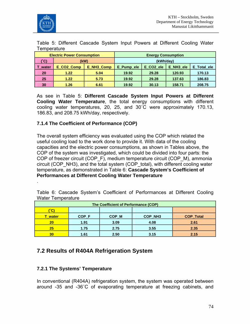
KTH – Stockholm, Sweden Department of Energy Technology Manustai Likitthammanit
74
Table 5: Different Cascade System Input Powers at Different Cooling Water Temperature
Electric Power Consumption Energy Consumption (˚C) (kW) (kWh/day)
T_water E_CO2_Comp E_NH3_Comp E_Pump_ele E_CO2_ele E_NH3_ele E_Total_ele 20 1.22 5.04 19.92 29.28 120.93 170.13 25 1.22 5.73 19.92 29.28 137.63 186.83 30 1.26 6.61 19.92 30.13 158.71 208.75
As see in Table 5: Different Cascade System Input Powers at Different Cooling Water Temperature, the total energy consumptions with different cooling water temperatures, 20, 25, and 30˚C were approximately 170.13, 186.83, and 208.75 kWh/day, respectively.
7.1.4 The Coefficient of Performance (COP) The overall system efficiency was evaluated using the COP which related the useful cooling load to the work done to provide it. With data of the cooling capacities and the electric power consumptions, as shown in Tables above, the COP of the system was investigated, which could be divided into four parts: the COP of freezer circuit (COP_F), medium temperature circuit (COP_M), ammonia circuit (COP_NH3), and the total system (COP_total), with different cooling water temperature, as demonstrated in Table 6: Cascade System’s Coefficient of Performances at Different Cooling Water Temperature . Table 6: Cascade System’s Coefficient of Performances at Different Cooling Water Temperature
The Coefficient of Performance (COP) (˚C)
T_water COP_F COP_M COP_NH3 COP_Total 20 1.91 3.09 4.08 2.61 25 1.75 2.75 3.55 2.35 30 1.61 2.50 3.15 2.15
7.2 Results of R404A Refrigeration System
7.2.1 The Systems’ Temperature In conventional (R404A) refrigeration system, the system was operated between around -35 and -36˚C of evaporating temperature at freezing cabinets, and
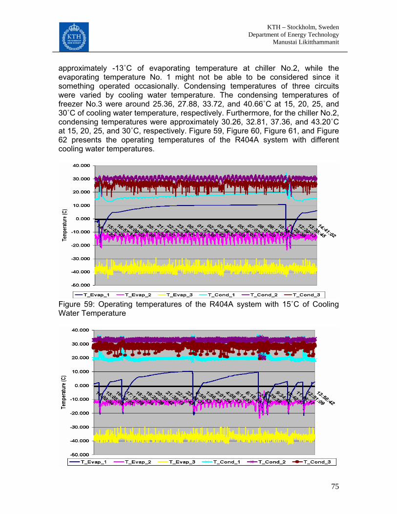
KTH – Stockholm, Sweden Department of Energy Technology Manustai Likitthammanit
75
approximately -13˚C of evaporating temperature at chiller No.2, while the evaporating temperature No. 1 might not be able to be considered since it something operated occasionally. Condensing temperatures of three circuits were varied by cooling water temperature. The condensing temperatures of freezer No.3 were around 25.36, 27.88, 33.72, and 40.66˚C at 15, 20, 25, and 30˚C of cooling water temperature, respectively. Furthermore, for the chiller No.2, condensing temperatures were approximately 30.26, 32.81, 37.36, and 43.20˚C at 15, 20, 25, and 30˚C, respectively. Figure 59, Figure 60, Figure 61, and Figure 62 presents the operating temperatures of the R404A system with different cooling water temperatures.
Figure 59: Operating temperatures of the R404A system with 15˚C of Cooling Water Temperature

KTH – Stockholm, Sweden Department of Energy Technology Manustai Likitthammanit
76
Figure 60: Operating temperatures of the R404A system with 20˚C of Cooling Water Temperature
Figure 61: Operating temperatures of the R404A system with 25˚C of Cooling Water Temperature
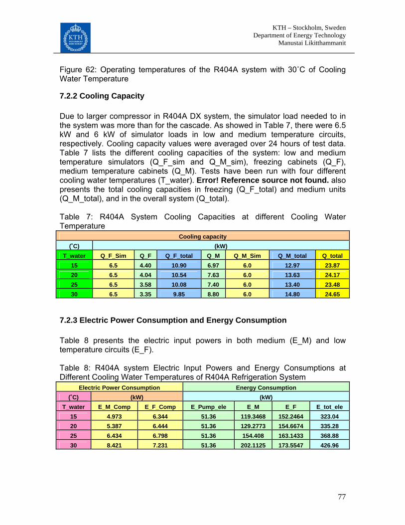
KTH – Stockholm, Sweden Department of Energy Technology Manustai Likitthammanit
77
Figure 62: Operating temperatures of the R404A system with 30˚C of Cooling Water Temperature
7.2.2 Cooling Capacity Due to larger compressor in R404A DX system, the simulator load needed to in the system was more than for the cascade. As showed in Table 7, there were 6.5 kW and 6 kW of simulator loads in low and medium temperature circuits, respectively. Cooling capacity values were averaged over 24 hours of test data. Table 7 lists the different cooling capacities of the system: low and medium temperature simulators (Q_F_sim and Q_M_sim), freezing cabinets (Q_F), medium temperature cabinets (Q_M). Tests have been run with four different cooling water temperatures (T_water). Error! Reference source not found. also presents the total cooling capacities in freezing (Q_F_total) and medium units (Q_M_total), and in the overall system (Q_total). Table 7: R404A System Cooling Capacities at different Cooling Water Temperature
Cooling capacity (˚C) (kW)
T_water Q_F_Sim Q_F Q_F_total Q_M Q_M_Sim Q_M_total Q_total 15 6.5 4.40 10.90 6.97 6.0 12.97 23.87 20 6.5 4.04 10.54 7.63 6.0 13.63 24.17 25 6.5 3.58 10.08 7.40 6.0 13.40 23.48 30 6.5 3.35 9.85 8.80 6.0 14.80 24.65
7.2.3 Electric Power Consumption and Energy Consumption Table 8 presents the electric input powers in both medium (E_M) and low temperature circuits (E_F). Table 8: R404A system Electric Input Powers and Energy Consumptions at Different Cooling Water Temperatures of R404A Refrigeration System
Electric Power Consumption Energy Consumption (˚C) (kW) (kW)
T_water E_M_Comp E_F_Comp E_Pump_ele E_M E_F E_tot_ele 15 4.973 6.344 51.36 119.3468 152.2464 323.04 20 5.387 6.444 51.36 129.2773 154.6674 335.28 25 6.434 6.798 51.36 154.408 163.1433 368.88 30 8.421 7.231 51.36 202.1125 173.5547 426.96

KTH – Stockholm, Sweden Department of Energy Technology Manustai Likitthammanit
78
7.2.4 The Coefficient of Performance (COP) Table 9 presents the COP of medium (COP_M), and low temperature circuits (COP_F), and the overall of the system (COP_total_ele). Table 9: R404A system COPs at Different Cooling Water Temperatures
The Coefficient of Performance (COP) (˚C)
T_water COP_M COP_F COP_total_ele 15 2.12 1.72 1.94 20 2.09 1.64 1.89 25 1.81 1.48 1.67 30 1.6 1.36 1.51
7.3 Results of Two Capacity Control Methods of NH3 Compressor Comparison
7.3.1 The System’s Temperature The new CO2 compressor and the new orifice, discussed earlier, were used for this test. The system was tested for three cooling water temperatures of 20, 25, and 30˚C with 4 hours period for each test point. The operating temperatures of the system in the two methods are presented in the tables below. The product temperatures in freezing cabinets were around -17.4 to -17.9˚C. On the other hand, in medium temperature cabinets product temperatures were about 2.5 and 2.8˚C. Evaporating temperatures were approximately -34 to -34.6 and -7.8 to -8˚C of low temperature and medium temperature circuits, respectively. Evaporating temperature of the ammonia unit, were about -10.7 to -11.3˚C. In the NH3 condenser, the condensing temperature is influenced by the cooling water temperature, which increased from 23.3 to 33˚C and from 23.2 to 33˚C for frequency and on-off controls when inlet water temperature increased from 20 to 30˚C. Table 10: Products and System Temperatures of NH3/CO2 Cascade System with Frequency Control of NH3 Compressor
Product Temp Evap Temp Cascade Cond Temp Cond Temp (˚C) (˚C) (˚C) (˚C) (˚C)
T_water T_F T_M T_F T_M T_CO2_Cond T_NH3_Evap dT_Cas Cond T_NH3_Cond 20 -17.43 2.54 -34.37 -7.97 -8.22 -10.74 2.51 23.29 25 -17.39 2.54 -34.18 -7.79 -8.03 -10.65 2.62 28.24 30 -17.42 2.56 -34.18 -7.81 -8.12 -10.70 2.58 32.98

KTH – Stockholm, Sweden Department of Energy Technology Manustai Likitthammanit
79
Table 11: Products and System Temperatures of NH3/CO2 Cascade System with On-Off Control of NH3 Compressor
Product Temp Evap Temp Cascade Cond Temp Cond Temp (˚C) (˚C) (˚C) (˚C) (˚C)
T_water T_F T_M T_F T_M T_CO2_Cond T_NH3_Evap dT_Cas Cond T_NH3_Cond 20 -17.65 2.74 -34.24 -7.78 -8.11 -11.25 3.14 23.17 25 -17.63 2.84 -34.11 -8.00 -8.32 -11.17 2.85 28.08 30 -17.87 2.77 -34.57 -7.78 -8.10 -11.02 2.92 32.95
7.3.2 Cooling Capacity, Electric Power Consumption, Energy Consumption and COP As shown in Table 12, the two simulator loads were set to 2 and 4.4 kW for low temperature and medium temperature levels, respectively. The time intervals between the tests were very short and the conditions in the laboratory were kept constant so the cooling capacities in both capacity control methods were similar. Electric power consumptions of for both control methods were measured and plotted in Figure 63. Furthermore, Table 13, Table 14, Table 15, and Table 16 present the electric power consumption, energy consumption and COP of tests for the two capacity control methods.
Figure 63: Electric Power Consumption of NH3 Compressor when Compressor Was Running with Frequency and On-Off Control Table 12: Cooling Capacities at Different Cooling Water Temperatures of the Cascade System with Frequency Control of the NH3 Compressor
Cooling capacity

KTH – Stockholm, Sweden Department of Energy Technology Manustai Likitthammanit
80
(˚C) (kW) T_water Q_F_sim Q_F Q_F_total Q_M Q_M_sim Q_M_total Q_Total Q_cadcade
20 2.00 3.68 5.68 8.65 4.40 13.05 18.72 20.75 25 2.00 3.74 5.74 8.31 4.40 12.71 18.45 20.45 30 2.00 3.40 5.40 7.30 4.40 11.70 17.10 19.06
Table 13: System’s Electric Power Consumption and Energy Consumption at Different Cooling Water Temperature of the Cascade System with Frequency Control of the NH3 Compressor
Electric Power Consumption Energy Consumption (˚C) (kW) (kWh/day)
T_water E_CO2_Comp E_NH3_Comp E_Pump_ele E_CO2_ele E_NH3_ele E_Total_ele 20 1.20 4.93 19.92 28.69 118.34 166.95 25 1.17 5.69 19.92 28.03 136.58 184.53 30 1.13 5.90 19.92 27.11 141.67 188.70
Table 14: System’s Electric Power Consumption and Energy Consumption at Different Cooling Water Temperature of the Cascade System with On-Off Control of the NH3 Compressor
Electric Power Consumption Energy Consumption (˚C) (kW) (kWh/day)
T_water E_CO2_Comp E_NH3_Comp E_Pump_ele E_CO2_ele E_NH3_ele E_Total_ele 20 1.20 4.96 19.92 28.69 118.96 167.58 25 1.17 5.71 19.92 28.03 137.10 185.05 30 1.13 6.39 19.92 27.11 153.48 200.51
Table 15: System’s Coefficient of Performance at Different Inlet Water Temperatures of the Cascade System with Frequency Control of the NH3 Compressor
The Coefficient of Performance (COP) (˚C)
T_water COP_F COP_M COP_NH3 COP_Total 20 2.02 3.16 4.21 2.69 25 1.87 2.76 3.59 2.40 30 1.73 2.48 3.23 2.18
Table 16: System’s Coefficient of Performance at Different Inlet Water Temperatures of the Cascade System with On-Off Control of the NH3 Compressor
The Coefficient of Performance (COP) (˚C)
T_water COP_F COP_M COP_NH3 COP_Total 20 2.01 3.15 4.19 2.68

KTH – Stockholm, Sweden Department of Energy Technology Manustai Likitthammanit
81
25 1.87 2.76 3.58 2.39 30 1.64 2.32 2.98 2.05
7.4 Transcritical CO2 Refrigeration System To compare the transcritical CO2 with NH3 unit, the evaporating pressure was kept at 26 bar (around -11˚C) by PID control which similar to the evaporating temperature of the NH3 unit. The high pressure was controlled by adjusting the opening of the expansion valve to find the optimum high pressure which results in the highest COP, as shown in Figure 8. The transcritical CO2 system was tested for four points of cooling water temperatures 15, 20, 25 and 30˚C. As a limitation for the maximum high pressure, the system was not tested for higher than 92 bar of discharge pressure. At 25˚C of cooling water temperature, the system was tested for four points of discharge pressure, 76, 82, 87, and 91 bar. While at 30˚C of cooling water temperature, the system was tested for three different discharge pressures, 86, 88, and 92 bar. Figure 64, Figure 65, Figure 66 and Figure 67 present the cooling capacity and electric input power, and COP in different high pressure at 25 and 30˚C of cooling water temperature, respectively.
Figure 64: Cooling Capacities and Electric Input Powers at 25˚C of Cooling Water Temperature at Different Discharge Pressures
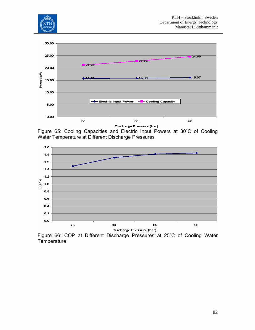
KTH – Stockholm, Sweden Department of Energy Technology Manustai Likitthammanit
82
Figure 65: Cooling Capacities and Electric Input Powers at 30˚C of Cooling Water Temperature at Different Discharge Pressures
Figure 66: COP at Different Discharge Pressures at 25˚C of Cooling Water Temperature

KTH – Stockholm, Sweden Department of Energy Technology Manustai Likitthammanit
83
Figure 67: COP at Different Discharge Pressures at 30˚C of Cooling Water Temperature At 15 and 20˚C of cooling water temperatures, the system was tested for five points of cooling water temperature. Figure 68 and Figure 69 present the cooling capacity and electric input power at 15 and 20˚C of cooling water temperatures. Figure 70 and Figure 71 show the COP of the system at different discharge pressures.
Figure 68: Cooling Capacities and Electric Input Powers at 15˚C of Cooling Water Temperature at Different Discharge Pressures
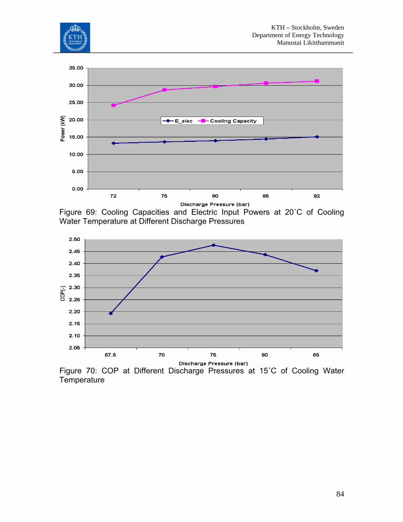
KTH – Stockholm, Sweden Department of Energy Technology Manustai Likitthammanit
84
Figure 69: Cooling Capacities and Electric Input Powers at 20˚C of Cooling Water Temperature at Different Discharge Pressures
Figure 70: COP at Different Discharge Pressures at 15˚C of Cooling Water Temperature

KTH – Stockholm, Sweden Department of Energy Technology Manustai Likitthammanit
85
Figure 71: COP at Different Discharge Pressures at 20˚C of Cooling Water Temperature In addition, from the heat balance, CO2 mass flow, the cooling capacities in each heat exchanger, input power and isentropic efficiency in both two stages of CO2 compressor could be investigated. Table 17 presents the intermediate pressure, which was around 52 bar, and the CO2 mass flow rate, which was about 0.143 to 0.145 kg/s at 15˚C of cooling water temperature. It also shows input power and isentropic efficiency of the first stage compressor, which were around 8.2 kW and 58%, respectively. At second stage, input power and isentropic efficiency were around 3 kW and 62%. In Table 18, the different kinds of heat exchangers’ capacities are listed. Table 17: Intermediate Pressure, CO2 Mass Flow Rate and CO2 Compressor Isentropic Efficiency Results at 15˚C of Cooling Water Temperature at Different Discharge Pressures
Bar M_CO2 Eta_k_1st E_1st Eta_k_2st E_2st HP MP Kg/s % kW % kW 85 52 0.145 57.04 8.26 70.13 3.84 80 52 0.144 57.53 8.14 66.47 3.55 75 52 0.144 58.22 8.08 62.21 3.22 70 54 0.144 59.52 8.26 57.57 2.63
67.5 53 0.143 59.94 8.15 54.16 2.45 Table 18: Capacities of system’s heat exchangers at 15˚C of Cooling Water Temperature at Different Discharge Pressures
Bar Q_Gascooler Q_MHEX Q_InHEX Q_OilCooler HP kW kW kW kW 85 31.12 9.70 1.04 1.43 80 30.56 9.40 1.06 1.41

KTH – Stockholm, Sweden Department of Energy Technology Manustai Likitthammanit
86
75 30.37 8.98 1.06 1.36 70 30.15 7.60 1.14 1.36
67.5 10.48 7.42 18.21 1.37 Similar tables as above are generated for 20, 25, 30˚C of cooling water temperature and presented as follows. Table 19: Intermediate Pressure, CO2 Mass Flow and CO2 Compressor Results at 20˚C of Cooling Water Temperature in Different Discharge Pressures
Bar M_C Eta_k_1st E_1st Eta_k_2st E_2st HP MP Kg/s % kW kW kW 92 54 0.141 57.22 8.48 74.53 4.05 85 53 0.142 58.06 8.35 71.26 3.71 80 53 0.142 58.56 8.26 67.53 3.37 75 54 0.140 58.11 8.33 63.87 2.96 72 54 0.139 58.77 8.25 59.88 2.68
Table 20: Capacities in Each Component at 20˚C of Cooling Water Temperature in Different Discharge Pressures
Bar Q_Gascooler Q_MHEX Q_InHEX Q_OilCooler HP kW kW kW kW 92 29.71 9.19 1.17 1.51 85 29.10 8.83 1.22 1.42 80 28.65 8.42 1.24 1.38 75 28.12 7.63 1.24 1.36 72 12.19 7.24 7.89 1.35
Table 21: Intermediate Pressure, CO2 Mass Flow and CO2 Compressor Results at 25˚C of Cooling Water Temperature in Different Discharge Pressures
Bar M_C Eta_k_1st E_1st Eta_k_2st E_2st HP MP Kg/s % kW % kW 90 55 0.142 56.83 8.87 76.29 3.89 86 54 0.141 57.45 8.75 73.65 3.62 80 55 0.141 57.69 8.75 69.65 3.20 76 55 0.141 58.21 8.77 66.35 2.85
Table 22: Capacities in Each Component at 25˚C of Cooling Water Temperature in Different Discharge Pressures
Bar Q_Gascooler Q_MHEX Q_InHEX Q_OilCooler HP kW kW kW kW 90 27.87 8.53 1.39 1.30 86 26.89 8.28 1.44 1.25 80 25.34 7.58 1.65 1.25 76 15.13 6.88 0.37 1.21

KTH – Stockholm, Sweden Department of Energy Technology Manustai Likitthammanit
87
Table 23: Intermediate Pressure, CO2 Mass Flow and CO2 Compressor Results at 30˚C of Cooling Water Temperature in Different Discharge Pressures
Bar m_C Eta_k_1st E_1st Eta_k_2st E_2st HP MP kg/s % kW % kW 92 57 0.147 56.29 9.73 74.27 4.15 88 57 0.147 56.38 9.68 72.17 3.95 86 57 0.149 55.95 9.74 71.13 3.80
Table 24: Capacities in Each Component at 30˚C of Cooling Water Temperature in Different Discharge Pressures
Bar Q_Gascooler Q_MHEX Q_InHEX Q_OilCooler High Pressure kW kW kW kW
92 28.713 7.574 1.655 1.228 88 27.021 7.447 1.742 1.254 86 25.721 7.182 1.957 1.244
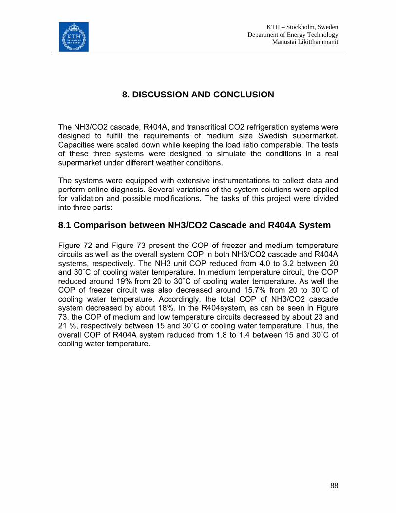
KTH – Stockholm, Sweden Department of Energy Technology Manustai Likitthammanit
88
8. DISCUSSION AND CONCLUSION
The NH3/CO2 cascade, R404A, and transcritical CO2 refrigeration systems were designed to fulfill the requirements of medium size Swedish supermarket. Capacities were scaled down while keeping the load ratio comparable. The tests of these three systems were designed to simulate the conditions in a real supermarket under different weather conditions. The systems were equipped with extensive instrumentations to collect data and perform online diagnosis. Several variations of the system solutions were applied for validation and possible modifications. The tasks of this project were divided into three parts:
8.1 Comparison between NH3/CO2 Cascade and R404A System Figure 72 and Figure 73 present the COP of freezer and medium temperature circuits as well as the overall system COP in both NH3/CO2 cascade and R404A systems, respectively. The NH3 unit COP reduced from 4.0 to 3.2 between 20 and 30˚C of cooling water temperature. In medium temperature circuit, the COP reduced around 19% from 20 to 30˚C of cooling water temperature. As well the COP of freezer circuit was also decreased around 15.7% from 20 to 30˚C of cooling water temperature. Accordingly, the total COP of NH3/CO2 cascade system decreased by about 18%. In the R404system, as can be seen in Figure 73, the COP of medium and low temperature circuits decreased by about 23 and 21 %, respectively between 15 and 30˚C of cooling water temperature. Thus, the overall COP of R404A system reduced from 1.8 to 1.4 between 15 and 30˚C of cooling water temperature.

KTH – Stockholm, Sweden Department of Energy Technology Manustai Likitthammanit
89
Figure 72: COPs of the NH3/CO2 Cascade System
Figure 73: COPs of the R404A System Performance comparisons of the two systems can be divided into three categories, the performance comparison of freezer circuit, medium temperature circuit, and overall system. In freezer circuit, the COP of NH3/CO2 cascade system was lower than R404A system, particularly at low cooling water temperature, as presented in Figure 74. At 20˚C of cooling water temperature, for instance, the COP of NH3/CO2 in freezing temperature circuit, which was 1.91, was higher than R404A system, which was 1.64. Furthermore, Figure 74 also

KTH – Stockholm, Sweden Department of Energy Technology Manustai Likitthammanit
90
illustrates the COP of medium temperature circuit in NH3/CO2 cascade system was much higher than R404A system.
Figure 74: The Performance Comparison of Freezer and Medium Temperature Circuits in NH3/CO2 Cascade and R404A System Figure 75 shows the COP comparison of low and medium temperature circuits in percentage. COPs of the cascade system are related, in percentages, to the values of the R404A system. As shown in Figure 75: COP Comparison in Percentage of Low and Medium Temperature Circuits, NH3/CO2 Cascade is related to R404A System Due to a large pumping power in the medium temperature circuit in R404A system, the COP was also compared without considering the pumping power in medium temperature circuits of both cascade and R404A systems. Figure 76 shows that the performance of medium temperature circuit in NH3/CO2 cascade system was still higher than R404A system by around 40-58%.

KTH – Stockholm, Sweden Department of Energy Technology Manustai Likitthammanit
91
Figure 76: The Performance Comparison of Medium Temperature Circuit in Percentage without Consideration of Pump Power , the COP of the low temperature circuit in the NH3/CO2 cascade system was higher than R404A system by around 17 and 18% at 20 and 30˚C of cooling water temperature. In medium temperature circuit, the COP of NH3/CO2 cascade system was much higher than R404A system, by about 70-80%.
Figure 75: COP Comparison in Percentage of Low and Medium Temperature Circuits, NH3/CO2 Cascade is related to R404A System Due to a large pumping power in the medium temperature circuit in R404A system, the COP was also compared without considering the pumping power in

KTH – Stockholm, Sweden Department of Energy Technology Manustai Likitthammanit
92
medium temperature circuits of both cascade and R404A systems. Figure 76 shows that the performance of medium temperature circuit in NH3/CO2 cascade system was still higher than R404A system by around 40-58%.
Figure 76: The Performance Comparison of Medium Temperature Circuit in Percentage without Consideration of Pump Power Figure 77 is a plot of the total system COP, it shows that the overall COP of NH3/CO2 cascade system was higher than the R404A system in all the tested cooling water temperature points.

KTH – Stockholm, Sweden Department of Energy Technology Manustai Likitthammanit
93
Figure 77: Total COP Comparison of NH3/CO2 Cascade and R404A Systems Furthermore, there are more explanations that why the cascade system has better performance than R404A system. At the medium temperature level, R404A system had to operate lower evaporating temperature than the cascade system since the R404A system had a superheat in evaporator and additional temperature difference in the heat exchange that connects the secondary loop with the primary. At 25 ˚C of cooling water temperature, for example, the evaporating temperature in medium temperature circuit of R404A system was around -16˚C, while it was about -8˚C in the cascade system. Consequently, R404A system consumed more power than the cascade system. Moreover, the pumping power of R404A system was an important factor to decrease the system’s performance since brine pump is usually larger than CO2 pump. Although load ratio for the cascade system was higher than R404A system, which means that R404A system could have been improved in terms total COP, the COP will not be improved much if the R404A system has more loads at medium temperature circuit. Based on the results and the above discussion it can be concluded that the NH3/CO2 cascade system has higher COP than the tested R404A system and it also proved to be a good alternative to R404A system for supermarket refrigeration.
8.2 Comparison of Two Speed Control Types of NH3 System The results show that NH3 compressor with on-off control consumed more electric input power than with frequency converter at high cooling water temperature as shown in Figure 78. At 30˚C of cooling water temperature, NH3 compressor with on-off control had around 8% higher electric power consumption than with frequency converter control. On the other hand, at 20˚C of cooling water temperature, the compressor had almost same power consumption in both control methods cases.
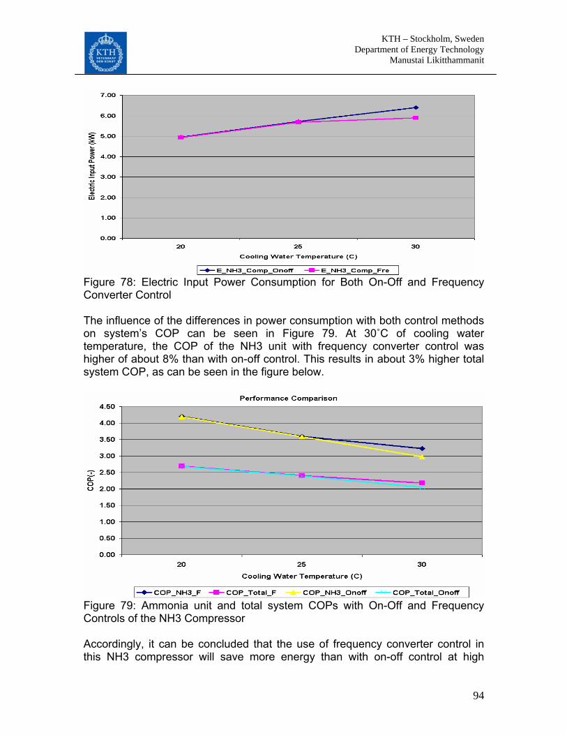
KTH – Stockholm, Sweden Department of Energy Technology Manustai Likitthammanit
94
Figure 78: Electric Input Power Consumption for Both On-Off and Frequency Converter Control The influence of the differences in power consumption with both control methods on system’s COP can be seen in Figure 79. At 30˚C of cooling water temperature, the COP of the NH3 unit with frequency converter control was higher of about 8% than with on-off control. This results in about 3% higher total system COP, as can be seen in the figure below.
Figure 79: Ammonia unit and total system COPs with On-Off and Frequency Controls of the NH3 Compressor Accordingly, it can be concluded that the use of frequency converter control in this NH3 compressor will save more energy than with on-off control at high
KTH – Stockholm, Sweden Department of Energy Technology Manustai Likitthammanit
95
ambient temperature. However to be installed in an actual plant, the economical factors need to be considered since frequency converter control is more expensive.
8.3 Comparison of Transcritical CO2 System and NH3/CO2 Cascade System In order to avoid any potential oil return problems in early runs of the system, the high stage CO2 system was tested without being connected to the low and medium temperature circuits, as shown in Figure 30. The PID controller maintained the evaporating pressure at 26 bar or 11˚C, which was used to compared to NH3 system in NH3/CO2 cascade system. The system was tested in four different cooling water temperatures, 15, 20, 25, and 30˚C. The result shows that 30˚C of cooling water temperature the maximum COP of the system could not be found due to limitations on discharge pressure of 100 bar. A reason for not identifying the optimum pressure might be that the CO2 compressor does not fit well for the operating temperature range, it was designed for low temperature application (below -20˚C). Theoretical optimum discharge pressure for heat sink temperatures of 30˚C is 88.4 bars. When the compressor operates at pressures higher than the theoretical optimum the isentropic efficiency increases which improves and COP and an optimum cannot be distinguished. Figure 80 presents the plot of test’s conditions at 30˚C of cooling water temperature with different discharge pressures, the black line show the theoretical optimum discharge pressure.

KTH – Stockholm, Sweden Department of Energy Technology Manustai Likitthammanit
96
-200 -100 05x101
9x101
h [kJ/kg]
P [b
ar]
35°C
30°C
CarbonDioxide
92 bars92 bars88 bars88 bars
86 bars86 bars
Pinter=57 bar
Popt=88,4 bar, Pinter;opt=56 barPopt=88,4 bar, Pinter;opt=56 bar
Tw=30°C
Figure 80: The plot of test’s conditions at 30 ˚C of cooling water temperature with different discharge pressures As well with the test at 25˚C of cooling water temperature, the maximum COP of the system could also not be found. Theoretical optimum discharge pressure for heat sink temperatures of 25˚C is about 75 bars. Figure 81 presents the plot of test’s conditions at 25˚C of cooling water temperature with different discharge pressures, the black line show the theoretical optimum discharge pressure.

KTH – Stockholm, Sweden Department of Energy Technology Manustai Likitthammanit
97
Figure 81: The plot of test’s conditions at 25 ˚C of cooling water temperature with different discharge pressures On the other hand, when the system operates sub-critically, there is no optimum COP. Thus at 15 and 20˚C of cooling water temperature, the system should operate with saturated liquid at the outlet of gas cooler and 2-3˚C of temperature difference in internal heat exchanger, as shown in black line of Figure 82 and Figure 83. Figure 82 and Figure 83 present the plot of test’s condition at 15 and 20˚C of cooling water temperature with different discharge pressures, respectively. A reason for different result between from experiment and theory might be the same reason as above that the CO2 compressor does not fit well for the operating temperature range.

KTH – Stockholm, Sweden Department of Energy Technology Manustai Likitthammanit
98
Figure 82: The plot of test’s conditions at 15 ˚C of cooling water temperature with different discharge pressures
Figure 83: The plot of test’s conditions at 20 ˚C of cooling water temperature with different discharge pressures
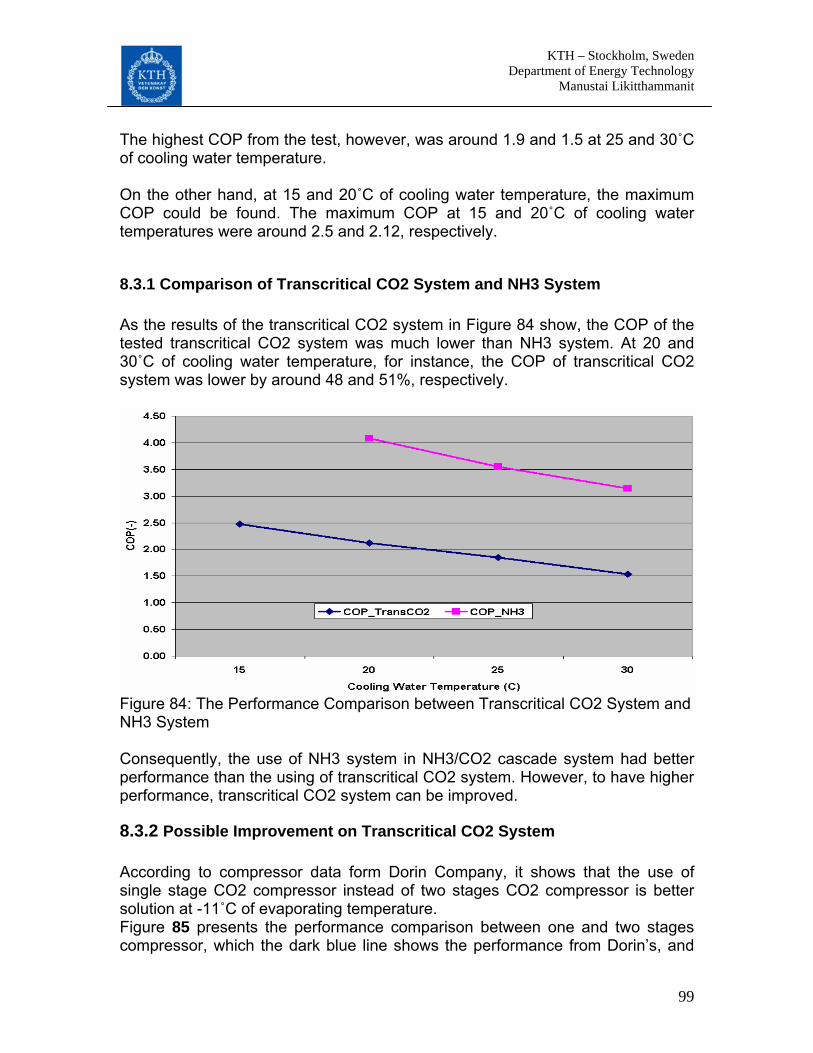
KTH – Stockholm, Sweden Department of Energy Technology Manustai Likitthammanit
99
The highest COP from the test, however, was around 1.9 and 1.5 at 25 and 30˚C of cooling water temperature. On the other hand, at 15 and 20˚C of cooling water temperature, the maximum COP could be found. The maximum COP at 15 and 20˚C of cooling water temperatures were around 2.5 and 2.12, respectively.
8.3.1 Comparison of Transcritical CO2 System and NH3 System As the results of the transcritical CO2 system in Figure 84 show, the COP of the tested transcritical CO2 system was much lower than NH3 system. At 20 and 30˚C of cooling water temperature, for instance, the COP of transcritical CO2 system was lower by around 48 and 51%, respectively.
Figure 84: The Performance Comparison between Transcritical CO2 System and NH3 System Consequently, the use of NH3 system in NH3/CO2 cascade system had better performance than the using of transcritical CO2 system. However, to have higher performance, transcritical CO2 system can be improved.
8.3.2 Possible Improvement on Transcritical CO2 System According to compressor data form Dorin Company, it shows that the use of single stage CO2 compressor instead of two stages CO2 compressor is better solution at -11˚C of evaporating temperature. Figure 85 presents the performance comparison between one and two stages compressor, which the dark blue line shows the performance from Dorin’s, and

KTH – Stockholm, Sweden Department of Energy Technology Manustai Likitthammanit
100
the yellow and pink line show the performance form estimated Dorin’s data. They were compared at 11˚C of evaporating temperature, 5˚C of temperature difference in gas cooler, 90 bar of high pressure and 35˚C of CO2 outlet temperature from gas cooler.
Figure 85: The Performance Comparison between Single and Two Stages CO2 Compressor from Dorin’s Compressor Data Using single stage CO2 compressor shows that the COP of the transcritical system can be increased by about 18.5% at 30 of cooling water temperature, shown in Figure 86. At 20˚C of cooling water temperature, for example, the COP with single stage compressor was improved by approximate 23%.

KTH – Stockholm, Sweden Department of Energy Technology Manustai Likitthammanit
101
Figure 86: COPs of Single-stage Transcritical, Two-Stage Transcritical and NH3 Systems With the use of transcritical CO2 system, CO2 from high stage can directly absorb heat in CO2 tank without cascade condenser, as shown in Figure 87. Thus, the evaporating temperature in transcritical CO2 system can be increased to -8˚C, which can reduce the input power to the compressor. Figure 88 shows the performance improvement of transcritical CO2 without cascade condenser. At 30˚C of cooling water temperature, for instance, the system without cascade condenser had better performance of about 6%. At 75 bar of high pressure, the performance can be improved by around 8.4% at 20˚C of cooling water temperature.

KTH – Stockholm, Sweden Department of Energy Technology Manustai Likitthammanit
102
Water5 kW
29 kWTranscritical CO2 System with Single Stage Compressor
Gas Cooler
Oil Seperator
Compressor
Internal HEX
CO2 tank
Figure 87: Schematic Diagram of the Transcritical CO2 System without Cascade Condenser
Figure 88: COPs of Single-stage Transcritical, Two-Stage Transcritical and NH3 Systems at Evaporating Temperature of -11°C and Single-stage Transcritical at Evaporating Temperature of -8°C
KTH – Stockholm, Sweden Department of Energy Technology Manustai Likitthammanit
103
With improvement of transcritical CO2 refrigeration system in terms of COP, the results show that the transcritical CO2 system still had lower performance than the NH3 system. Consequently, the use of tested NH3 system in cascade CO2 is better solution than the transcritical CO2 system in terms of COP. However, there are important factors, such as cost of components, leakage rates, amount of charge, and heat recovery, which have to be considered to find the best solution for refrigeration in supermarkets.

KTH – Stockholm, Sweden Department of Energy Technology Manustai Likitthammanit
104
9. REFERENCES [1] Annex 31 Advanced Modeling and Tools for Analysis of Energy Use in Supermarket Systems, IEA Heat Pump Centre, SP Swedish National Testing and Research Institute. [2] Arias, J., Energy Usage in Supermarkets Modelling and Field Measurements, Doctoral thesis, Department of Energy Technology, Royal Institute of Technology, Stockholm, Sweden, (2005). [3] Cambell, A., Maidment, G.G. and Missenden, J.F., A Natural Refrigerant System for Supermarkets using CO2 as a Refrigerant, CIBSE National Conference, (March 2006) [4] Granryd, E., Ekroth, I., Ludqvist, P., Melinder, Ǻ., Palm, B., and Rohlin, P., Refrigeration Engineering, Department of Energy Technology, KTH, Stockholm, Sweden, (2003). [5] Kim G. Christensen and P.Bertilsen, Danish Technological Institute and Danfoss, Refrigeration Systems in Supermarkets with Propane and CO2 –Energy Consumption and Economy, the 2003 International Congress of Refrigeration. [6] Gerrit Jan v. Reissen, M.Sc. TNO Environmental and Process Innovation, NH3/CO2 supermarket refrigeration system with CO2 in the cooling and freezing section, Holland utan datering [7] Kim, M.-H., et al., Fundamental Process and System Design Issues in CO2 Vapor Compression Systems, Department of Mechanical Engineering, Korea Advanced Institute of Science and Technology, South Korea, (2003). [8] Sawalha, S., Soleimani,A., Rogstam,J., CO2 in Supermarket Refrigeration - 1st phase report. 2006, IUC, (Dec 2005). [9] Pierluigi Schiesaro and Horst Kruse, Development of a two stage CO2 supermarket system, R&D Deparment ARNEG S.p.A 35020, Campo San Marino, Italy [10] Petter Neksa, CO2 as Refrigerant for Systems in Transcritical Operation Principles and Technology SINTEF Energy Research, NO-7465, Trondheim, NORWAY, (Sep 2004) [11] Denso, World First CO2 Air Conditioning System, Toyota Motor Show 2003 [12] Linda, First CO2 Refrigeration System for Medium and Low Temperature Refrigeration at Swiss Mega Store, (Feb 2005) [13] Horst Kruse, Rainer Jakobs, and Hans Russmann , On the energy efficiency of carbon dioxide in small commercial cooling applications, Forschungszentrum für Kältetechnik und Wärmepumpen GmbH, Hannover, Germany [14] Yamasaki, H. et al.: Introduction of Transcritical Refrigeration Cycle Utilizing CO2 as Working Fluid.17th International Compressor Engineering Conference at Purdue. 2004.
KTH – Stockholm, Sweden Department of Energy Technology Manustai Likitthammanit
105
[15] Veje, C., Süss, J.: The Transcritical CO2 Cycle in Light Commercial Refrigeration Applications. 6th Gustav Lorentzen Conference, Glasgow.2004. [16] IEA Heat Pump Newsletter Volume 23 No.2/2005 [17] Hans Hammer, Carbon Dioxide (R 744) as supplementary heating device, AUDI AG, (July 2000) [18] Experimental investigations of an automotive heat pump prototype for military, SUV and compact car, 4th IIR-Gustav Lorentzen conference [19] Tamura, Yakumaru, and Nishiwaki, Experimental study on automotive cooling and heaing air-conditioning system using CO2 as refrigerant, Osaka, Japan, (Nov 2005) [20] Carlos Perales Cabrejas, Parametric Evaluation of a NH3/CO2 cascade system for supermarket refrigeration in laboratory environment, Master of science thesis in refrigeration, Department of Energy and Technology, KTH, Sweden, (2006) [21] Dorin Innovation, CO2 Range paper; Available from: www.dorin.com (2006-12-11) [22] SuperMax Plate Heat Exchanger & Heat Exchangers; Available from: www.tranter.com (2006-12-02) [23] Shujun Wang, Modeling and experimental investigation of accumulators for automotive air conditioning systems, International Journal of Refrigeration, 2006 [24] Trygve M. Eikevik, Ingvald Strømmen, Odilio Alves-Filho, Heat Pump Fluidised Bed Dryer with CO2 as Refrigerant – Measurements of COP and SMER, Norwegian University of Science and Technology (NTNU)