Experimental investigations and simulations of the control ...
17
3 rd European supercritical CO2 Conference September 19-20, 2019, Paris, France 2019-sCO2.eu-148 EXPERIMENTAL INVESTIGATIONS AND SIMULATIONS OF THE CONTROL SYSTEM IN SUPERCRITICAL CO2 LOOP Ales Vojacek* Research Centre Řež Řež, Czech Republic [email protected] Tomas Melichar Research Centre Řež Řež, Czech Republic Petr Hajek Research Centre Řež Řež, Czech Republic Frantisek Doubek Research Centre Řež Řež, Czech Republic Timm Hoppe XRG Simulation GmbH Hamburg, Germany ABSTRACT An efficient instrumentation and control system (I&C), which is adaptable to loads variations (temperature, pressure, mass flow), is essential for design of power units working with supercritical CO2 (sCO2) to ensure high sCO2 cycle performance with quick response. Hence, sophisticated model- based control system design, supported by dynamic system- level modelling, simulations, and experimental verification is needed. This technical paper presents experimental tests and numerical simulations of the control system of the experimental supercritical CO2 loop at Research Centre Rez (CVR), Czech Republic. The measurements covered testing of temperature, pressure and mass flow controllers. Set-up of the controllers and dynamic response of the system are investigated for several transient scenarios in supercritical and subcritical pressures including transition of the pseudocritical region. The experimental set-up along with the boundary conditions are described in detail, hence the gained data set can be used for benchmarking of system thermal hydraulic codes. Such a benchmarking was performed with the open source Modelica- based code ClaRa using the simulation environment DYMOLA 2019. INTRODUCTION The power cycle using sCO2 is an innovative concept which is a competitive alternative to the dominated steam Rankine cycle, gas Brayton cycle or their combination. The sCO2 cycles have a clear potential to attain comparable or even higher cycle efficiencies than conventional steam Rankine/ or Brayton gas cycles [1], [2]. The sCO2 combine many advantages of both the steam Rankine cycle (minimizing the power requirement for compressing the working fluid + heat rejection at low temperatures) and Brayton gas cycle (small size, modular design, fast built units). It also achieves a high degree of thermal recuperation as both Brayton and Rankine cycles. The research activities on sCO2 power plants are progressively increasing during the last decades and there is a growing interest in the worldwide sCO2 events as well. It certainly shows a significant market potential. A report by Sandia Nat. Lab. [3] claims the prospective is to bring the sCO2 cycle to technical readiness level 6 (till 2020) paving the way to demonstration projects (from 2020) and to commercialization (from 2025). The outlook is in line with the testimony of currently running sCO2 projects in Europe, e.g. sCO2-Flex [4]. A number of investigators have carried out extensive experimental tests and analyses of sCO2. However, their work is rather limited to the component behavior studies, i.e. heat transfer and pressure drop models in heaters/coolers/heat exchangers [5], [6], [7]. An exhaustive literature survey on research in supercritical heat transfer is reported in [8]. Very few data can be found on operation and analysis of compressors and turbines [1], [9]-[13]. This is due to the fact that first prototypes of turbomachines are being just built. What is missing is simulation tool which is validated on models of the system level (component interaction) on both steady states and dynamic transients including control system interactions. The main objective of this work is to provide evidence that the open source Modelica-based code ClaRa [14] is suitable for modeling steady states and transient scenarios along with Proportional Integral Derivative (PID) controllers’ actions and their tuning in sCO2 environment. For this purpose, CVR has performed number of experimental tests in the sCO2 facility, located in CVR in the Czech Republic. As a part of experimental campaign, three steady states were selected (covering different temperature levels and pressures) in order to benchmark the numerical model at first place. A set of relevant parameters are given later in the text along with a detailed description of the experimental facility (loop geometry, nominal DOI: 10.17185/duepublico/48916
Transcript of Experimental investigations and simulations of the control ...

3rd
European supercritical CO2 Conference
September 19-20, 2019, Paris, France
2019-sCO2.eu-148
EXPERIMENTAL INVESTIGATIONS AND SIMULATIONS OF THE CONTROL
SYSTEM IN SUPERCRITICAL CO2 LOOP
Ales Vojacek*
Research Centre Řež
Řež, Czech Republic
Tomas Melichar
Research Centre Řež
Řež, Czech Republic
Petr Hajek
Research Centre Řež
Řež, Czech Republic
Frantisek Doubek
Research Centre Řež
Řež, Czech Republic
Timm Hoppe
XRG Simulation GmbH
Hamburg, Germany
ABSTRACT
An efficient instrumentation and control system (I&C),
which is adaptable to loads variations (temperature, pressure,
mass flow), is essential for design of power units working with
supercritical CO2 (sCO2) to ensure high sCO2 cycle
performance with quick response. Hence, sophisticated model-
based control system design, supported by dynamic system-
level modelling, simulations, and experimental verification is
needed. This technical paper presents experimental tests and
numerical simulations of the control system of the experimental
supercritical CO2 loop at Research Centre Rez (CVR), Czech
Republic. The measurements covered testing of temperature,
pressure and mass flow controllers. Set-up of the controllers
and dynamic response of the system are investigated for several
transient scenarios in supercritical and subcritical pressures
including transition of the pseudocritical region. The
experimental set-up along with the boundary conditions are
described in detail, hence the gained data set can be used for
benchmarking of system thermal hydraulic codes. Such a
benchmarking was performed with the open source Modelica-
based code ClaRa using the simulation environment DYMOLA
2019.
INTRODUCTION
The power cycle using sCO2 is an innovative concept
which is a competitive alternative to the dominated steam
Rankine cycle, gas Brayton cycle or their combination. The
sCO2 cycles have a clear potential to attain comparable or even
higher cycle efficiencies than conventional steam Rankine/ or
Brayton gas cycles [1], [2]. The sCO2 combine many
advantages of both the steam Rankine cycle (minimizing the
power requirement for compressing the working fluid + heat
rejection at low temperatures) and Brayton gas cycle (small
size, modular design, fast built units). It also achieves a high
degree of thermal recuperation as both Brayton and Rankine
cycles. The research activities on sCO2 power plants are
progressively increasing during the last decades and there is a
growing interest in the worldwide sCO2 events as well. It
certainly shows a significant market potential. A report by
Sandia Nat. Lab. [3] claims the prospective is to bring the sCO2
cycle to technical readiness level 6 (till 2020) paving the way to
demonstration projects (from 2020) and to commercialization
(from 2025). The outlook is in line with the testimony of
currently running sCO2 projects in Europe, e.g. sCO2-Flex [4].
A number of investigators have carried out extensive
experimental tests and analyses of sCO2. However, their work
is rather limited to the component behavior studies, i.e. heat
transfer and pressure drop models in heaters/coolers/heat
exchangers [5], [6], [7]. An exhaustive literature survey on
research in supercritical heat transfer is reported in [8]. Very
few data can be found on operation and analysis of compressors
and turbines [1], [9]-[13]. This is due to the fact that first
prototypes of turbomachines are being just built. What is
missing is simulation tool which is validated on models of the
system level (component interaction) on both steady states and
dynamic transients including control system interactions.
The main objective of this work is to provide evidence that
the open source Modelica-based code ClaRa [14] is suitable for
modeling steady states and transient scenarios along with
Proportional Integral Derivative (PID) controllers’ actions and
their tuning in sCO2 environment. For this purpose, CVR has
performed number of experimental tests in the sCO2 facility,
located in CVR in the Czech Republic. As a part of
experimental campaign, three steady states were selected
(covering different temperature levels and pressures) in order to
benchmark the numerical model at first place. A set of relevant
parameters are given later in the text along with a detailed
description of the experimental facility (loop geometry, nominal
DOI: 10.17185/duepublico/48916

2 DOI: 10.17185/duepublico/48916
pressures, temperatures, heating power and mass flow rate, etc.)
to allow preparation of the computational models.
Once the numerical model was cross-checked, the tuning
procedure of the PID controllers was performed. There are
number of different control loops in the sCO2 loop at CVR.
However, as the control mode is most often associated with
temperature, hence the temperature controller at the outlet of
the heater 2 (H2) was selected to be subject of this work. Many
various tuning methods have been proposed from 1942 up to
now for gaining better and more acceptable control system
response based on our desirable control objectives such as
percent of overshoot, integral of absolute value of the error,
settling time, manipulated variable behavior and etc. One of the
most common PID controller tuning technique used in industry
was consolidated and evaluated both from experimental data as
well as from the numerical model. The tuning method chosen
was the Cohen-Coon method [15] where process dynamics is
based on a first order plus deadtime model. The tuning settings
was calculated using the Cohen-Coon rules [16] and
implemented in both real and Modelica controller. Afterwards,
several tests were carried out in order to ensure the response is
in line with the overall control objective of the loop.
Above mentioned procedure was conducted for a specific
thermal hydraulic condition (pressure, temperature) in the
sCO2 experimental loop. For linear processes, where the
process characteristics do not change significantly with time or
load conditions, then using the set fixed PID parameters will
probably be sufficient to ensure effective control. In the case of
non-linear processes, however, being limited to a single set of
fixed parameters can become problematic. One would need to
set the parameters for the worst case, i.e. giving a very low
gain, not to cause instabilities in higher gain conditions. In
order to find the best overall response, independent sets of PID
parameters are needed. Hence, numbers of tests with different
conditions were executed with numerical models and different
PID sets were derived. Finally, the new sets were implemented
in the numerical model and checked for improvements in the
control of a process.
The presented results in this paper will benefit to
researchers, designers, software engineers, thermal hydraulic
specialists, and operators of sCO2 energy systems through the
shared measured data in a unique sCO2 facility.
DESCRIPTION OF THE LOOP AND GEOMETRY
SPECIFICATIONS
The sCO2 experimental loop at CVR was constructed
within SUSEN (Sustainable Energy) project in 2017. This
unique facility enables component testing of sCO2 Brayton
cycle such as compressor, turbine, HX, valves and to study key
aspects of the cycle (heat transfer, erosion, corrosion etc.) with
wide range of parameters: temperature up to 550°C, pressure up
to 30 MPa and mass flow rate up to 0.35 kg/s. The loop is
designed to represent sCO2 Brayton cycle behavior.
Although the sCO2 loop characteristics are not
prototypical of the foreseen sCO2 power plant, the experiments
on this simplified facility is sufficient to assess the capability of
the numerical codes to deal with the thermal-hydraulic behavior
of the sCO2 loop. One of the adaptation of the loop is that a
radial compressor expected on the prospective sCO2 power
plant is substituted by a piston type pump. In addition, a turbine
is replaced by a reduction valve.
Annex A shows the piping and instrumentation diagram
(PID) of the loop. The primary circuit is marked in thick red
and it consists of following main components:
The piston-type main pump (MP), which circulates
sCO2 through the circuit with the variable speed drive
for the flow rate control.
The high and low temperature regenerative heat
exchangers (HTR HX/LTR HX), which recuperate the
heat, hence reduce the heating and cooling power.
The 4 electric heaters (H1/1, H1/2, H2, H3), which
have in total a maximum power of 110 kW and raise
the temperature of sCO2 to the desired test section
(TS) inlet temperature up to 550°C.
The reduction valve which consists of series of orifices
to reduce the pressure and together with oil
(Marlotherm SH) cooler (CH2) represent a turbine.
The water cooler (CH1) cools down the sCO2 at the
inlet of the MP by water cooling circuit. The
secondary water cooling circuit is cooled by tertiary
water cooling circuit. PI&D of the sCO2 loop does not
depict tertiary water cooling circuit for simplification
matter of the benchmark exercise. The complete sets
of boundary conditions are defined for the secondary
water cooling circuit allowing this reduced approach.
Air driven filling (reciprocating) compressor (gas
booster station) which pumps the sCO2 from the CO2
bottles and also controls the operating pressure.
Exhaust system for the excess amount of sCO2
The P&ID of the sCO2 loop contains all installed key
measurement devices, such as a mass flow meter, Pt-100
sensors, thermocouples, pressure sensors and wattmeters.
The nomenclature of the measurement devices respects the
KKS identification system for power plants.
The uncertainties provided by the measurement
devices, transducer, input card, and control system are
summarized in Annex B. The errors correspond to
calibration certificates and manufacturer’s instructions.
Just for a matter of clarity, the zig-zag line at the P&ID
stands for the oil cooler CH2 and connected pipeline. This
line was closed during testing campaign since it was not
needed to have extra cooling power in oil cooling circuit.
The main operating parameters of the primary circuit
are shown in Table 1.
Table 1: The main operating parameters of the sCO2 primary
loop.
Maximum operation pressure 25 MPa
Maximum pressure 30 MPa
Maximum operation 550°C

3 DOI: 10.17185/duepublico/48916
temperature
Maximum temperature in HTR 450°C
Maximum temperature in LTR 300°C
Nominal mass flow 0.35 kg/s
The sCO2 loop layout is depicted in Figure 1 and the top
view of the built facility is shown in Figure 2.
Figure 1: 3D CAD model of the sCO2 loop.
Figure 2: A view from the top on the built sCO2 loop.
Table 2 summarizes parameters of the MP and the
schematic cross-section of the MP is shown in Figure 3.
Table 2: Parameters of the main pump.
Device Main Pump - PAX-3-30-
18-250-YC-CRYO-drive
9/FM
Nominal inlet pressure 12.5 MPa
Nominal outlet pressure 25 MPa
Maximal outlet pressure 30 MPa
Nominal inlet temperature 25°C
Maximum inlet temperature 50°C
Nominal isentropic efficiency 0.7
Rotational speed (manufacturer
data)
250÷1460 rpm
Volumetric flowrate
(manufacturer data)
5÷30 l/min.
Rotational speed -> Volumetric
flowrate (measurement data)
555 rpm -> 9.8 l/min
935 rpm -> 16.7 l/min
Figure 3: Cross-section of main pump.
In Table 3, the main parameters of the filling compressor
are listed.
Table 3: Parameters of the filling compressor.
Device Filling compressor - DLE5-15-
GG-C
Nominal inlet pressure of
CO2
0.5 MPa
Nominal outlet pressure 6.5 MPa
Maximum outlet pressure 30 MPa
Nominal flowrate 15 standard litre per minute
Nominal air pressure 0.6 MPa
Geometric parameters of the heat exchanging components
of the sCO2 loop needed for preparation of the model are
described in
Annex C. The parameters needed for the model settings
such as pipe diameters and lengths, layouts of heat exchangers
and heaters and materials are listed for each component
according to PI&D scheme in the Annex A.
The geometry of HTR heat exchangers is demonstrated in
Figure 4. It is a counter-current shell and tube heat exchanger
and it concludes of 2 U-tube modules. The LTR heat exchanger
is of a same type and it includes 6 U-tube modules.

4 DOI: 10.17185/duepublico/48916
Figure 4: HTR heat exchanger.
The geometry of the tube plate LTR/HTR heat exchanger
of inserted in a shell is displayed in Figure 5.
Figure 5: LTR/HTR heat exchanger tube plate in a shell.
The cross cut of electrical heater rod of H1/1, H1/2, H2 and H3
is shown in Figure 6.
Figure 6: Electrical heater rod cross cut.
The cross cut of electrical heaters of H1/1, H1/2 H3 are
shown in Figure 7 and H2 in Figure 8. All heaters are equipped
with guiding tube Ø 36 x 2 mm which directs the flow around
the electrical heater rods. This tube is plugged on both ends.
Figure 7: Electrical heater H1/1, H1/2 and H3 cross cut.
Figure 8: Electrical heater H2 cross cut.
The electrical heater H3 with nominal power 20 kW is
positioned at the bypass of the LTR in order to simulate the
behavior of a recompression cycle.
The pressure loss coefficients of the valves related to cross-
section areas of corresponding pipelines (inner diameter 14
mm) are listed in Table 4.
Table 4: Pressure loss coefficient of the fully-open valves
Valve type Pressure loss coefficient [-]
Reduction valve
(characteristic in Table 5) 827
Control valves
(linear characteristic) 14
Closing valves
(“hot” part of the loop) 12
Closing valves
(“cold” part of the loop) 4
The reduction valve characteristic Opening versus Kv/Kvs
of the reduction valve is displayed in Table 5. Averaged values
of Kv/Kvs from all measured data covering temperature range
50°C ÷ 450°C are given (no data from manufacturer are
available).
Table 5: Characteristic of the of the reduction valve.
Opening [%] Kv/Kvs [-]
0 0.09
40.5 0.45
45 0.52
50 0.59
55 0.65
60 0.70
65 0.74
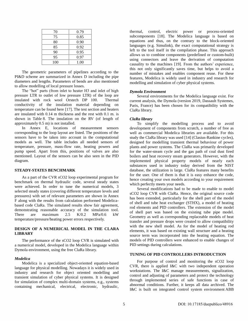
5 DOI: 10.17185/duepublico/48916
70 0.79
75 0.85
80 0.90
85 0.92
90 0.95
95 0.97
100 1.00
The geometric parameters of pipelines according to the
PI&D scheme are summarized in Annex D including the pipe
diameters and lengths. Parameters of bends are also mentioned
to allow modelling of local pressure losses.
The “hot” parts (from inlet to heater H3 and inlet of high
pressure LTR to outlet of low pressure LTR) of the loop are
insulated with rock wool Orstech DP 100. Thermal
conductivity of the insulation material depending on
temperature can be found here [17]. The test section and heaters
are insulated with 0.14 m thickness and the rest with 0.1 m. is
shown in Table 8. The insulation on the RV (of length of
approximately 0.5 m) is not installed.
In Annex E, locations of measurement sensors
corresponding to the loop layout are listed. The positions of the
sensors have to be taken into account in the computational
models as well. The table includes all needed sensors of
temperature, pressure, mass-flow rate, heating powers and
pump speed. Apart from this, positions of valves are also
mentioned. Layout of the sensors can be also seen in the PID
diagram.
STEADY-STATES BENCHMARK
As a part of the CVR sCO2 loop experimental program for
benchmark on thermal hydraulic code, several steady states
were achieved. In order to tune the numerical models, 3
selected steady states (covering different temperature levels and
pressures) with set of relevant parameters are shown in Annex
F along with the results from calculation performed Modelica-
based code ClaRa. The simulated results show fair agreement,
demonstrating reasonable accuracy of the simulation tool.
There are maximum 2.5 K/0.2 MPa/0.6 kW
temperature/pressure/heating power errors respectively.
DESIGN OF A NUMERICAL MODEL IN THE CLARA
LIBRARY
The performance of the sCO2 loop CVR is simulated with
a numerical model, developed in the Modelica language within
Dymola environment, using the free ClaRa library.
Modelica
Modelica is a specialized object-oriented equation-based
language for physical modelling. Nowadays it is widely used in
industry and research for object oriented modelling and
transient simulation of cyber physical systems. It is designed
for simulation of complex multi-domain systems, e.g., systems
containing mechanical, electrical, electronic, hydraulic,
thermal, control, electric power or process-oriented
subcomponents [18]. The Modelica language is based on
equations and thus, on the contrary to the block-oriented
languages (e.g. Simulink), the exact computational strategy is
left to the tool itself in the compilation phase. This approach
allows us to combine components (predefined or custom-built)
using connectors and leave the derivation of computation
causality to the machines [19]. From the authors’ experience,
this not only significantly saves time, but helps to avoid a
number of mistakes and enables component reuse. For these
features, Modelica is widely used in industry and research for
modelling and simulation of cyber physical systems.
Dymola Environment
Several environments for the Modelica language exist. For
current analysis, the Dymola (version 2019, Dassault Systemes,
Paris, France) has been chosen for its compatibility with the
ClaRa library.
ClaRa library
To simplify the modelling process and to avoid
development of components from scratch, a number of free as
well as commercial Modelica libraries are available. For this
study the ClaRa library was used [14] (Clasius-Rankine cycles),
designed for modelling transient thermal behaviour of power
plants and power systems. The ClaRa was primarily developed
for the water-steam cycle and the gas path of coal dust fired
boilers and heat recovery steam generators. However, with the
implemented physical property models of nearly each
substances used in industry today derived from the NIST
database, the utilization is large. ClaRa features many benefits
for the user. One of them is that it is easy enhance the code,
hence creating your own models according to your requirement
which perfectly meets your needs.
Several modifications had to be made to enable to model
sCO2 loop CVR with ClaRa. Hence, the original source code
has been extended, particularly for the shell part of the model
of shell and tube heat exchanger (STHX), a model of heating
rod elements and PID controllers. The extension of the model
of shell part was based on the existing tube pipe model.
Geometry as well as corresponding replaceable models of heat
transfer and pressure drops were created to allow compatibility
with the new shell model. As for the model of heating rod
elements, it was based on existing wall structure and a heating
source term was incorporated into the heating equation. The
models of PID controllers were enhanced to enable changes of
PID settings during calculations.
TUNING OF PID CONTROLLERS INTRODUCTION
For purpose of control and monitoring the sCO2 loop
CVR, there is applied I&C with two independent operation
workstations. The I&C manage measurements, signalization,
control and adjusting of parameters and protect the technology
through implemented series of safe functions in case of
abnormal conditions. Further, it keeps all data archived. The
I&C is built on integrated control system environment ABB

6 DOI: 10.17185/duepublico/48916
FREELANCE with ABB – AC900F control units and S800 I/O
[21] modules directly attached on terminal units (for binary
signals) and Siemens ET200M (for analog signals) [22].
Accurate control is critical to every process. As a means of
ensuring that tasks such as production, distribution and
treatment processes are carried out under the right conditions
for the right amount of time and in the right quantities, control
devices form a crucial part of virtually every industrial process.
Currently the PID algorithm is the most popular feedback
controller used in industry. Having a three term functionality
that deals with transient and steady-state responses, the PID
controller offers a simple, inexpensive, yet robust algorithm
that can provide excellent performance, despite the varied
dynamic characteristics of the process or plant being controlled
[23]. To get the best out of the PID controllers, many tuning
techniques have been developed over the past several decades.
The very first techniques are dated to 1942 when Ziegler and
Nichols published their paper. They have come with a closed-
loop and open-loop method. The principles of these methods
still provide the foundation of many of the auto tune algorithms
used in many modern industrial applications. Despite its
simplicity, the Ziegler Nichols closed loop method can take a
long time to perform and also has the potential to create
uncontrolled oscillations, which affects control stability. Eleven
years after Ziegler and Nichols published their findings, in
1953, Cohen and Coon published a new tuning method. Like
the Ziegler-Nichols open loop rules, the Cohen-Coon rules aim
for a quarter-amplitude damping response. The Cohen-Coon
tuning rules are suited to a wider variety of processes than
the Ziegler-Nichols tuning rules. The Ziegler-Nichols rules
work well only on processes where the dead time is less
than half the length of the time constant. The Cohen-Coon
tuning rules work well on processes where the dead time
is less than two times the length of the time constant (and it can
be stretched even further if required) [16]. Hence, the Cohen-
Coon method has been used in this paper.
It is often forgotten or simply not known that different
tuning rules were developed for different versions of the PID
controller algorithm. The engineer responsible for tuning a
control loop must be aware of the form of the algorithm used
for the PID controller. The main PID structures (Interactive,
Non-interactive and parallel) are very well described in [16].
The Cohen-Coon rule, used in this paper, utilizes the Non-
interactive algorithm. The algorithm is described in equation
(1).
𝑪𝑶 = 𝑲𝒄 ∙ (𝒆(𝒕) +𝟏
𝑻𝒊∫ 𝒆(𝒕) 𝒅𝒕 + 𝑻𝒅
𝒅𝒆(𝒕)
𝒅𝒕) (1)
The Cohen-Coon tuning rule uses three process
characteristics: process gain (GP), dead time (td), and time
constant (Tau). These are determined by doing a step test and
analyzing the results. In order to derive these characteristics,
the PID controller which is subject of the tuning needs to be in
manual and the system has to be stabilized. A step change in the
controller output (CO) is introduced and after the process
variable (PV) stabilizes at a new value, the characteristics can
be determined according to Figure 9. The size of this step
should be large enough that the process variable moves well
clear of the process noise/disturbance level.
Figure 9: Schematic figure of Cohen-Coon characteristics.
Calculation of new tuning settings using the Cohen-Coon
tuning rule is described in Table 6.
Table 6: Cohen-Coon rule [16]. Kc Ti Td
P controller 1.03
𝐺𝑃(
𝑇𝑎𝑢
𝑡𝑑+ 0.34)
PI controller 0.9
𝐺𝑃(
𝑇𝑎𝑢
𝑡𝑑+ 0.092) 3.33𝑡𝑑 (
𝑇𝑎𝑢 + 0.092𝑡𝑑
𝑇𝑎𝑢 + 2.22𝑡𝑑)
PD
controller
1.24
𝐺𝑃(
𝑇𝑎𝑢
𝑡𝑑+ 0.129) 0.27𝑡𝑑 (
𝑇𝑎𝑢 − 0.324𝑡𝑑
𝑇𝑎𝑢 + 0.129𝑡𝑑)
PID
controller
1.35
𝐺𝑃(
𝑇𝑎𝑢
𝑡𝑑+ 0.185) 2.5𝑡𝑑 (
𝑇𝑎𝑢 + 0.185𝑡𝑑
𝑇𝑎𝑢 + 0.611𝑡𝑑) 0.37𝑡𝑑 (
𝑇𝑎𝑢
𝑇𝑎𝑢 + 0.185𝑡𝑑)
One has to be careful when calculating the process gain GP
according to equation (2), since normalized values needs to be
implemented, i.e. the total change obtained in PV has to be
converted to a percentage of the span of the measuring device.
Similarly to the change of CO in percentage.
𝑮𝑷 = 𝒄𝒉𝒂𝒏𝒈𝒆 𝒊𝒏 𝑷𝑽 [%]
𝒄𝒉𝒂𝒏𝒈𝒆 𝒊𝒏 𝑪𝑶 [%](2)
TUNING OF PID CONTROLLERS AND COMPARISON
WITH MEASSURED DATA
There are number of different control loops in the sCO2
loop at CVR. However, as the control mode is most often
associated with temperature, hence the temperature controller at
the outlet of the heater 2 (H2) was selected to be subject of this
work.
As described in previous chapter, the Cohen-Coon method
is used in this paper to determined PID controller constant. Two
step changes in the heater 2 (H2) during a stabilized system
were introduced and process variable (T_CO2_H2_out -
1LKD40CT004) curves have been generated.
Step-up
Firstly, a sudden step-up increase in H2 power output
(from initial 6.2 kW to final 10.9 kW) was initiated at stable
system. The response curve of the process variable
(temperature outlet from H2) is shown in Figure 10.

7 DOI: 10.17185/duepublico/48916
Figure 10: Response curve of temperature outlet from H2
during step-up test.
Step-down
In order to verify the first test, second step test was
conducted after the stabilization of parameters in the system. A
sudden step-down decrease in H2 power output (from initial
10.9 kW to final 6.6 kW) was initiated at stable system. The
response curve of the process variable (temperature outlet from
H2) is shown in Figure 11.
Figure 11: Response curve of temperature outlet from H2
during step-down.
In both cases, the simulated results from the ClaRa model
follows the measured values of the process variable very well.
The total maximum error calculated from absolute temperatures
in Kelvins, does not exceeds 0.5 %.
Table 7 summarizes the PID tuning settings from both tests
including the settings derived from simulations. Note that
calculated controller gain (Kc) is according to recommendation
[16] divided the by two to reduce overshoot and improve
stability. For clarity, the process gain (GP) was calculated as
follows (the step-up experimental values are shown):
𝑮𝑷 =
𝒄𝒉𝒂𝒏𝒈𝒆 𝒊𝒏 𝑷𝑽 [𝑲]
𝒓𝒂𝒏𝒈𝒆 𝒐𝒇 𝑷𝑽 [𝑲]
𝒄𝒉𝒂𝒏𝒈𝒆 𝒊𝒏 𝑪𝑶 [𝒌𝑾]
𝒓𝒂𝒏𝒈𝒆 𝒐𝒇 𝑪𝑶 [𝒌𝑾]
=𝟏𝟓𝟓.𝟑− 𝟏𝟑𝟎
𝟔𝟎𝟎−𝟎𝟏𝟎.𝟗 −𝟔.𝟐
𝟑𝟎−𝟎
= 𝟎. 𝟐𝟕 (3)
Table 7: PID tuning settings for measured and simulated
data
Kc Ti Td
Step-up test – measured 29.14 5.60 0.85
Step-down test - measured 26.79 5.97 0.90
Average - measured 27.96 5.79 0.88
Step-up test – simulated 26.79 5.35 0.81
Step-down test - simulated 26.33 5.24 0.79
Average - simulated 26.56 5.30 0.80
The PID constants obtained from both experimental tests
are in very good agreement. The discrepancy of the PID sets
derived from simulations and experiment is within 10%. One of
the possible explanation for error results from the fact that the
dead time for both test cases are relatively small (around 2.2 s),
hence even a small error (of few tenths of seconds) in
determination the dead time from the tangent line at inflection
point can lead to significant inaccuracy in the PID constants.
In order to provide complete data for benchmark exercises,
all relevant parameters of the sCO2 loop CVR at steady state
conditions, prior to the step changes, are summarized in
ANNEX G. In addition, the simulated results are shown,
providing further evidence about the capability of the numerical
code capturing the measured values.
TUNING OF PID CONTROLLERS FOR MULTIPLE
PROCESS CONDITIONS
Fluid properties of the sCO2 near the critical point
experiences highly non-linear variations. This is one of the key
enabling features for the sCO2, however on the other hand, it
presents challenges for modeling, and exhibits unique behavior
during transients which greatly complicate the control of the
system. To demonstrate that series of response curves with
different conditions (pressure 10 MPa ÷ 20 MPa, temperature
30 °C ÷ 400 °C) were simulated and tuning constants of the
PID controller were derived using Cohen-Coon method for
each case. Once again, the temperature outlet from heater H2
was selected as a process variable. Notice that the parametric
values of pressures stated here are meant to be pressures at the
heater H2 where the response test took place, i.e. high pressure
side of the loop (from outlet of the main circulation pump to
reduction valve). Further, mass flow rate through the sCO2 loop
was kept constant at 0.13 kg/s and so do the low pressure
values (7.65 MPa) to maintain a core of similarity with the PID
tuning in the previous chapter. Hence, 10 MPa at the high
pressure side was the minimum value for a given low pressure
7.65 MPa taking into account the pressure losses through the
loop.
The resulted tuned controller gains (Kc) for different
conditions in the sCO2 loop are plotted in Figure 12. Since the
120
130
140
150
160
0 20 40 60 80 100 120
Tem
per
atu
re [°C
]
Time [s]
PID - Tuning- Temp_H2_out_Step_Up
T_measurement
tangent
T_simmulation
InflectionPoint
120
130
140
150
160
0 20 40 60 80 100 120
Tem
per
atu
re [°C
]
Time [s]
PID - Tuning- Temp_H2_out_Step_Down
T_measurement
tangent
T_simmulation
InflectionPoint

8 DOI: 10.17185/duepublico/48916
integral and derivative time constants did not varied
significantly and stayed in a relatively small range (Ti = 4 s ÷ 6
s and Td = 0.6 s ÷ 1 s), they are not shown here explicitly. From
the Figure 12 it can be observed that the controller gains follow
the behavior of heat capacity. The specific heat capacity (cp) is
peaking at so called pseudo-critical temperatures and similarly
the controller gains. This effect is growing closer it gets to the
critical pressure. The behavior of controller gains can be
explained as follows. Where the cp is higher, there the PID
controller needs higher gain in order to have sufficiently fast
response. On the other hand, where cp is smaller, there the PID
controller needs lower gain not to cause oscillations. Note that
controller gains are gain divided the by two to reduce overshoot
and improve stability.
Figure 12: Calculated values of controller gains and specific
heat capacities at different pressures and temperatures.
Once the new sets of PID controller were derived, they
were tested on several examples. Following figures Figure 13,
Figure 14 and Figure 15 shows the behavior of PID controller
of the temperature outlet from H2 during the step change of set
point. For demonstration, two extreme PID sets were chosen
together with manually tuned constants. One extreme case
represents the parameters tuned for the highest cp approx. 8
kJ·kg-1
·K-1
(Kc=118, Ti=3.7 s, Td=0.6 s) and the other for the
lowest cp approx. 1 kJ·kg-1
·K-1
(Kc=25, Ti=5 s, Td=1 s). Both
were derived from previous calculation tuned by Cohen-Coon
method. For the manually tuned PID following constants were
used (Kc=25, Ti=20 s, Td=1 s), i.e. the setting was the same as
for the case with the lowest cp, only the integral time constant
quadrupled.
Figure 13: Outlet temperatures of H2 at 10MPa controlled by
PID with different settings (set point at 45°C).
Figure 14: Outlet temperatures of H2 at 10MPa controlled by
PID with different settings (set point at 100°C).
Figure 15: Outlet temperatures of H2 at 10MPa controlled by
PID with different settings (set point at 400°C).
0
20
40
60
80
100
120
140
0
1
2
3
4
5
6
7
8
9
30 80 130 180
Kc[
-]
cp[k
J/kg
K]
T[°C]
cp at 10 MPa
cp at 15 MPa
cp at 20 MPa
Kc at 10 MPa
Kc at 15 MPa
Kc at 20 MPa
40
45
50
55
60
0 20 40 60 80 100 120
Tem
per
atu
re [°C
]
Time [s]
T_tuned_for_high_cp
T_tuned_for_low_cp
T_tuned_manual
set point
90
95
100
105
110
115
120
0 20 40 60 80
Tem
per
atu
re [°C
]
Time [s]
T_tuned_for_high_cp
T_tuned_for_low_cp
T_tuned_manual
set point
390
395
400
405
410
415
420
0 20 40 60
Tem
per
atu
re [°C
]
Time [s]
T_tuned_for_high_cp
T_tuned_for_low_cp
T_tuned_manual
set point

9 DOI: 10.17185/duepublico/48916
It can be observed that the process variable, controlled by
PID with settings tuned for high cp, exhibits comparatively
high overshoots and instabilities, especially for the higher
temperatures test cases (above 100°C). Improvement can be
seen for the low cp tuning. It still exhibits quite high
overshoots, however the oscillations were significantly
reduced. The manually tuned controller behaves well for all 3
tested temperatures. It shows no overshoots, no oscillations,
only for the test at 45°C, time for the process variable to settle
is quite long (100 s) and it could be improve by increasing the
controller gain.
CONCLUSION
The paper shows a comprehensive insight into the
experimental investigations and simulations of the sCO2 loop
in CVR. Rather than focusing on separate component behavior,
this study aims on a system level (component interaction) for
both steady states and dynamic transients including control
system interactions and PID tuning techniques. Particularly, this
paper contains valuable experimental data of the sCO2 loop and
their comparison with simulations.
The first part of the paper presents the sCO2 loop, and
shows its configuration and specifications. This includes the
design parameters of all main components as well as the P&I
diagram with measurements and their positions in the system
and the piping. Altogether three sets of measured steady states
data are outlined and together with detail description of the
loop it gives necessary information for performing the
benchmark exercise on numerical codes. Such a benchmark
was performed with the open source Modelica-based code
ClaRa using the simulation environment DYMOLA 2019. The
simulated results show fair agreement with measured data,
demonstrating reasonable accuracy of the simulation tool.
There are maximum 2.5 K/0.2 MPa/0.6 kW
temperature/pressure/heating power errors respectively. Further
measurements and simulations were carried out, particularly
transients, however it is out of the page limit for the paper.
Hence, the results of these analyses will be published
somewhere else.
Once the numerical model on steady states was validated,
the transient tests covering the tuning procedure of the PID
controllers were performed. The scope of the study is to give a
first approximation of tuning parameters of such a system. For
this purpose, one of the most utilized tuning technique, the
Cohen-Coon (C-C) method, was deployed. The temperature
controller at the outlet of the heater 2 (H2) was selected to be
subject of this work. A sudden step-up/step-down
increase/decrease in H2 power output respectively at a given
condition was executed. The response temperature curves were
analyzed and PID constants for the controller were calculated.
The PID constants obtained from both experimental tests are in
very good agreement. The discrepancy of the PID sets derived
from simulations and experiment is within 10%.
For the sake of highly non-linear behavior of sCO2, series
of response curves with different conditions (pressure 10 MPa
÷ 20 MPa, temperature 30 °C ÷ 400 °C) were simulated in
order to find the optimum PID settings for all prospective
conditions for sCO2 loop in CVR. It was observed that the
resulted controller gains follow behavior of the specific heat
capacity, hence they were peaking at the pseudocritical points.
This naturally intensifies closer it gets to the supercritical
pressure. Hence, near the pseudocritical temperatures and
supercritical pressures the PID would need to be given various
customized sets of constants for particular conditions. Far from
the pseudocritical temperatures, single PID setting should be
sufficient.
Once the new sets of PID controller were derived, they
were tested on several examples. It has been found that the
tuned PID constants according to C-C method exhibits
relatively high overshoots. It is due to the fact that different
tuning techniques gives preferences to fast response prior to
stable behavior. The results from the paper indicates that C-C
method prefers fast response. Hence, if one would like to use
sole set of PID for all different conditions then it is
recommended to use the settings tuned for lower values of cp,
i.e. with lower controller gain. Otherwise, the system might
oscillates in low cp regions. One has to understand that derived
PID constants according to C-C method are just first
approximations and further manual tuning are inevitable. In this
paper the manually tuned parameters were based on the C-C
tuning setting for low cp case and only the integral time
constant was quadrupled. With this PID setting the performance
of the controller was very much improved with practically
representative actions.
Further investigations are planed including deployment of
several other tuning techniques in order to improve predictions
of the PID settings. In addition, other control loops of the sCO2
experimental facility in CVR, i.e. mass flow through the cycle
driven by circulation pump with frequency convertor or
pressure in the system driven by reduction valve etc., are
prospective to be tested.
NOMENCLATURE
cp Specific heat capacity, J·kg-1
·K-1
D Diameter, m
e(t) Error (Set point – Process variable)
H Enthalpy, J·kg-1
Kc Controller gain
Kv Flow coefficient of the valve, m3·h
-1
Kvs Kv at a fully-open valve position, m3·h
-1
L Length, m
m Mass flow, kg·s-1
p Pressure, Pa
P Power, W
T Temperature, K
Ti Integral time constant
Td Derivative time constant
ρ Density, kg·m-3

10 DOI: 10.17185/duepublico/48916
ACRONYMS
C-C Cohen-Coon
CH1 Water cooler
CH2 Oil cooler
CO Control output signal of PID controller
GP Process gain
H1/1 Electric heater
H1/2 Electric heaters
H2 Electric heaters
H3 Electric heaters
HP High pressure
HTR High temperature regenerative heat exchanger
I&C Instrumentation and control system
KKS Identification system for power plants
LP Low pressure
LTR Low temperature regenerative heat exchanger
MP Main pump
PID Proportional Integral Derivative
P&ID Piping and instrumentation diagram
PV Process value
RV Reduction valve
sCO2 Supercritical CO2
td Dead time (time difference between the change in CO
and the intersection of the tangential line and the
original PV level)
Tau Time constant (time difference between intersection at
the end of dead time, and the PV reaching 63% of its
total change)
STHX Shell and tube heat exchanger
ACKNOWLEDGEMENTS
This paper has been conducted within the sCO2-Flex
project which has received funding from the European Union’s
Horizon 2020 research and innovation programme under grant
agreement N° 764690.
REFERENCES
[1] DOSTAL V.: A supercritical carbon dioxide cycle for
next generation nuclear reactors [Ph.D. thesis]. Department of
Nuclear Engineering, Massachusetts Institute of Technology
(MIT); 2004.
[2] BRUN K.; FRIEDMAN P.; DENNIS R.:
Fundamentals and Applications of Supercritical Carbon
Dioxide (SCO2) Based Power Cycles. 1st edition, Elsevier
Science & Technology, 2017.
[3] MENDEZ, C.M., ROCHAU G.: sCO2 Brayton Cycle: Roadmap to sCO2 Power Cycles NE Commercial Applications,
SANDIA REPORT, SAND2018-6187, Printed June 2018,
Albuquerque, New Mexico.
[4] CAGNAC, A., 2018, “The supercritical co2 cycle for
flexible & sustainable support to the electricity system (sco2-
flex),” Electricité de France, Avenue de Wagram 22, 75008,
Paris 08, Accessed Apr. 4, 2019, http://www.sco2-flex.eu/.
[5] BRINGER, R.P.; SMITH, J.M.: Heat transfer in the
critical region. AIChE J. 3 (1), 49–55, 1957.
[6] PETUKHOV, B.S.; KRASNOSCHEKOV, E.A.;
PROTOPOPOV, V.S.: An investigation of heat transfer to fluids
flowing in pipes under supercritical conditions. In: International
Developments in Heat Transfer: Papers presented at the 1961
International Heat Transfer Conference, ASME, University of
Colorado, Boulder, Colorado, USA, 8–12 January, Part III,
Paper 67, pp. 569–578, 1961.
[7] DUFFEY, R.B.; PIORO, I.L.: Experimental heat
transfer of supercritical carbon dioxide flowing inside channels
(survey), Nuclear Engineering and Design 235 (2005) 913–924.
[8] VOJACEK, A. ET AL.: Challenges in supercritical
CO2 power cycle technology and first operational experience at
CVR, 2nd European sCO2 Conference, Duisburg-Essen,
August 2018, DOI: 10.17185/duepublico/46075.
[9] WRIGHT, S.A. ET AL.: Operation and Analysis of a
Supercritical CO2 Brayton Cycle, SAND2010-0171,
Albuquerque, New Mexico, Sep. 2010.
[10] UTAMURA, M. ET. AL.: Demonstration of
supercritical CO2 closed regenerative brayton cycle in a bench
scale experiment. Proceedings of ASME Turbo Expo 2012,
June 11-15, 2012, Copenhagen, Denmark, GT2012-68697.
[11] HACKS A. J.; VOJACEK A.; DOHMEN H. J.;
BRILLERT D.: Experimental Investigation of the sCO2-HeRo
Compressor. 2018-sCO2.eu-115, 2nd European supercritical
CO2 Conference, August, 2018.
[12] AHN, Y. ET. AL.: Design consideration of
supercritical CO2 power cycle integral experiment loop, Energy
86 (2015) 115-127.
[13] CHO, J. ET. AL.: Research on the development of a
small-scale supercritical carbon dioxide power cycle
experimental test loop, The 5th International Symposium -
Supercritical CO2 Power Cycles, March 28-31, 2016, San
Antonio, Texas.
[14] NIELSEN, L.: TLK-Thermo GmbH,
“Dyncap/Dynstart | ClaRa – Simulation of Clausius-Rankine
cycles | TLK-Thermo GmbH, Braunschweig | XRG Simulation
GmbH, Hamburg | Institut für Thermofluiddynamik (TUHH),
Hamburg | Institut für Energietechnik (TUHH), Hamburg.”
[Online]. Available: https://www.claralib.com/. [Accessed: 4-
Apr-2019].
[15] COHEN, G. H.; G. A. COON (1953): "Theoretical
consideration of retarded control."Trans. ASME, 75, pp. 827-
834.
[16] SMUTS, J.F.: Control notes – Reflection of a process
control practitioner. [Online]. Available:
http://blog.opticontrols.com. [Accessed: 4-Apr-2019].
[17] Division Isover, Saint-Gobain Construction Products
CZ a.s., Masarykova 197, 517 50 Častolovice. [Online].

11 DOI: 10.17185/duepublico/48916
Available: https://www.isover.cz/en/products/orstech-dp-100. .
[Accessed: 4-Apr-2019].
[18] CASELLA F.; LEVA, A.: “Modelling of thermo-
hydraulic power generation processes using Modelica,” Math.
Comput. Model. Dyn. Syst., vol. 12, no. 1, pp. 19–33, Feb.
2006.
[19] KOFRANEK, J. ET. AL.: “Causal or acausal
modeling: labour for humans or labour for machines,” in
Technical Computing Prague, 2008, pp. 1–16.
[20] NIST Reference Fluid Thermodynamic and Transport
Properties Database (REFPROP): Version 10.
[21] Ulrich Spiesshofer, ABB Asea Brown Boveri Ltd,
Affolternstrasse 44, 8050 Zurich, Switzerland Available:
https://new.abb.com/control-systems/essential-
automation/freelance. [Accessed: 4-Apr-2019].
[22] Siemens Aktiengesellschaft Werner-von-Siemens-
Straße 1, 80333 Munich, Germany Available:
https://w3.siemens.com/mcms/distributed-io/en/ip20-
systems/et200m/interface-modules/pages/default.aspx.
[Accessed: 4-Apr-2019].
[23] LI, Y.; ANG, K.H.; CHONG, G.C.Y. (2006) PID
control system analysis and design. IEEE Control Systems
Magazine 26(1):pp. 32-41.
[24] ZIEGLER, J. G.; NICHOLS, N.B.: “Optimum
Settings for Automatic Controllers,” Transactions of the ASME,
Vol. 64, 1942, pp. 759-768.

12 DOI: 10.17185/duepublico/48916
ANNEX A
PIPING AND INSTRUMENTATION DIAGRAM (P&ID) OF THE SCO2 LOOP, CVR
ANNEX B
UNCERTAINTY OF THE MEASUREMENT DEVICES IN SCO2 LOOP, CVR
Variable Range Unit Description Device
error
Transducer error Input card
error
Control system
error
Total error
msCO2 0 - 0.7 kg/s mass flow rate
1LKB10CF001,
1LKB70CF00 1Rheonik (RHM12)
0.15 %
from 1.66
kg/s
Rawet - PX310S Siemens
SM 331
ABB freelance +/- 0.007 kg/s
0.1 % from range 0.4 % from
range
0.1 % from
range
T_sCO2 0 - 600 °C TC (type K) T_sCO2, Omega
+/- 0.5 K for
(0÷100°C)
+/- 0.6 K for
300°C
+/- 1.4 K for
500°C
Rawet - PX310S Siemens SM 331
ABB freelance +/- 4.1 K for (0÷100°C)
+/- 4.2 K for
300°C +/- 5 K for 500°C
0.1 % from range 0.4 % from
range
0.1 % from
range
p_sCO2_LP 0 - 15 MPa sCO2 pressures at low pressure side of
0.15 % from range
Rawet - PX310S Siemens SM 331
ABB freelance +/- 0.11 MPa

13 DOI: 10.17185/duepublico/48916
the loop, GE (UNIK
5000)
0.1 % from range 0.4 % from
range
0.1 % from
range
p_sCO2_HP 0 - 30 MPa sCO2 pressures at high pressure side of
the loop , GE
(UNIK 5000)
0.15 % from range
Rawet - PX310S Siemens SM 331
ABB freelance +/- 0.23 MPa
0.1 % from range 0.4 % from range
0.1 % from range
P_H1/1-2
P_H2,3 0 - 30 kW electric power of
heaters, MT Brno 0.75 %
from range Rawet - PX310S Siemens
SM 331 ABB freelance +/- 0.4 kW
0.1 % from range 0.4 % from range
0.1 % from range
T_water 0 - 120 °C water temperature of
the cooling circuit, JSP (Pt 100)
0.15K+0.2
% from range
Rawet - PX310S Siemens
SM 331
ABB freelance +/- 1.1 K
0.1 % from range 0.4 % from range
0.1 % from range
mwater 0 – 3.8 kg/s water mass flow rate
of the cooling circuit, turbine
flowmeter, Hoffer
1.1 % from
range
- - ABB freelance +/- 0.046 kg/s
- - 0.1 % from
range
ANNEX C
UNCERTAINTY OF THE MEASUREMENT DEVICES IN SCO2 LOOP, CVR
Component Geometry
HTR + LTR
(counter-flow shell and tube-type from SS 321)
Length of HTR = 20 m (2 x U-tube vertical), 3 x 2 = 6 high pressure flanges Ø 110 mm (height 25 mm) and the same 6 low
pressure flanges Length of LTR = 60 m (6 x U-tube vertical), 7 x 2 = 14 high pressure flanges Ø 110 mm (height 25 mm) and the same 14
low pressure flanges
Number of internal tubes = 7, Internal tube Ø 10 x 1.5 mm, Shell Ø 50 x 5 mm.
H1/1 + H1/2 (30 + 30 kW)
(from SS 321)
Length = 0.95 m, Number of heating rods = 2 x 6, Diameter of a heating rod Ø 8 mm (cladding tube Ø 8 x 1 mm SS 321, ceramic (MgO) filling Ø 6 x 1 mm, ceramic (Al2O3) filling Ø 4 x 1.75 mm, Ø 0.5 mm wire Kanthal alloy (FeCrAl)), Shell
Ø 100 x 20 mm, guiding tube Ø 36 x 2 mm with plugs on both ends
H2
(30 kW) (from Inconel 625)
Length = 0.95 m, Number of heating rods = 2 x 6, Diameter of a heating rod 8 mm (ceramic filling and wire as in H1/1 +
H1/2), Shell Ø 73 x 6.5 mm, 2 x 1 = 2 flanges Ø 110 mm (height 25 mm), guiding tube Ø 36 x 2 mm with plugs on both ends
H3
(20 kW)
(from SS 321)
Length = 0.75 m, Number of heating rods = 2 x 6, Diameter of a heating rod Ø 8 mm (ceramic filling and wire as in H1/1 +
H1/2), Shell Ø 100 x 20 mm, guiding tube Ø 36 x 2 mm with plugs on both ends
CH1 (counter-flow shell and tube-type from
SS)
Length = 7.5 m, Number of internal tubes = 7, Internal tube Ø 10 x 1.5 mm, Shell Ø 43 x 1.5 mm
CH2
(counter-flow shell and tube-type from Inconel 625 (CO2 side)/SS 321 (oil
side))
Length = 1.8 m, Number of internal tubes = 7, Internal tube Ø 10 x 1.5 mm, Shell Ø 43 x 1.5 mm, 2 x 2 = 4 high flanges Ø
110 mm (height 25 mm)
TS (from Inconel 625)
Length = 2 m, Shell Ø 73 x 6.5 mm, 2 x 2 = 4 high flanges Ø 140 mm (height 26 mm)
Reduction valve
(from SS 321)
Body weight 125 kg, Length = 0.5 m
Control valves (3x)
(from SS 321)
Body weight 5 kg, Length = 0.3 m
(each)
Closing valves Body weight 1 kg, Length = 0.3 m

14 DOI: 10.17185/duepublico/48916
*(“hot” part of the loop)
(from SS 321)
(each)
Closing valves
**(“cold” part of the loop) (from SS 321)
Body weight 5 kg, Length = 0.3 m
(each)
* The “hot” part of the loop is from inlet of heater H3 and inlet of high pressure LTR to outlet of low pressure LTR.
** The “cold” part is the rest of the loop (from outlet of low pressure LTR to inlet to heater H3 and inlet of high pressure LTR.
ANNEX D
PIPELINE GEOMETRY OF THE SCO2 LOOP
Line 1 Pipeline from MP to T-junction LTR by-pass Length = 2.6 m, 1x90° Bend, Tube Ø 22 x 4 mm
Line 2 Pipeline from T-junction LTR by-pass to LTR Length = 6.8 m, 6x90° Bend, Tube Ø 22 x 4 mm
Line 3 LTR by-pass Length = 7.6 m, 2x90° Bend, Tube Ø 22 x 4 mm
Line 4 Pipeline from outlet of high pressure LTR to inlet of high pressure HTR Length = 0.7 m, 2x90° Bend, Tube Ø 22 x 4 mm
Line 5 Pipeline from outlet of high pressure HTR to T-junction at the inlet of H1/1 and H1/2 Length = 1 m, 1x90° Bend, Tube Ø 22 x 4 mm
Line 6a/6b 2 identical pipelines from T-junction at the inlet of H1/1 and H1/2 to H1/1 and H1/2 Length = 1.4 m, 1x60° Bend, Tube Ø 22 x 4 mm
Line 7a/7b 2 identical pipelines from H1/1 and H1/2 to T-junction at the outlet of H1/1 and H1/2 Length = 1.5 m, 1x60° Bend, Tube Ø 22 x 4 mm
Line 8 Pipeline from T-junction outlet of H1/1 and H1/2 to H2 Length = 1.9 m, 2x90° Bend, Tube Ø 22 x 4 mm
Line 9 Pipeline from H2 to test section Length = 2 m, 2x90° Bend, Tube Ø 22 x 4 mm
Line 10 Pipeline from test section to reduction valve Length = 1.9 m, 1x90° Bend, Tube Ø 22 x 4 mm
Line 11 Pipeline from reduction valve to T-junction of line 12a/13 Length = 8.4 m, 8x90° Bend, Tube Ø 20 x 3 mm
Line 12a Pipeline from T-junction of line 12a/13 to T-junction CH2 by-pass (inlet of CH2 by-pass) Length = 0.4 m, 1x60° Bend, Tube Ø 20 x 3 mm
Line 12b Pipeline from T-junction CH2 by-pass (inlet of CH2 by-pass) to T-junction of line 12b/13 Length = 0.4 m, 1x60° Bend, Tube Ø 20 x 3 mm
Line 13 Pipeline from T-junction of line 12a/13 to T-junction of line 12b/13 to Length = 0.9 m, 2x60° Bend, Tube Ø 20 x 3 mm
Line 14 Pipeline CH2 by-pass Length = 5.5 m, 4x90° Bend, Tube Ø 20 x 3 mm
Line 15a Pipeline from T-junction of line 15a/16 to T-junction CH2 by-pass (outlet of CH2 by-pass) Length = 0.4 m, 1x60° Bend, Tube Ø 20 x 3 mm
Line 15b Pipeline from T-junction CH2 by-pass (outlet of CH2 by-pass) to T-junction of line 15b/16 Length = 0.4 m, 1x60° Bend, Tube Ø 20 x 3 mm
Line 16 Pipeline from T-junction of line 15a/16 to T-junction of line 15b/16 Length = 0.9 m, 2x60° Bend, Tube Ø 20 x 3 mm
Line 17 Pipeline from T-junction of line 15b/16 to inlet of low pressure HTR Length = 0.8 m, 1x90° Bend, Tube Ø 20 x 3 mm
Line 18 Pipeline from outlet of low pressure HTR to inlet of low pressure LTR Length = 0.7 m, 2x90° Bend, Tube Ø 22 x 4 mm
Line 19 Pipeline from outlet of low pressure LTR to CH1 Length = 1.8 m, 2x90° Bend, Tube Ø 20 x 3 mm
Line 20 Pipeline from CH1 to MP Length = 4.4 m, 7x90° Bend, Tube Ø 20 x 3 mm
ANNEX E
POSITION OF THE MEASUREMENT SENSORS
Measurement type Position Pipeline
m_CO2_MP (1LKB70CF001) 3.9 m prior to MP inlet line 20
m_CO2_LTR (1LKB10CF001) 1.6 m from MP outlet line 1
rotational speed_MP (1LKC10CS001) MP line 1
power_H1/1 (1LKD40CE011A) H1/1 line 6b,7b
power_H1/2 (1LKD40CE011B) H1/2 line 6a,7a
power_H2 (1LKD40CE011C) H2 line 8,9
power_H3 (1LKD10CE011) H3 line 3
p_CO2_MP_in (1LKB70CP001) 3.4 m prior to MP inlet line 20
T_CO2_MP_in (1LKB70CT001) 5.1 m prior to MP inlet line 20
p_CO2_MP_out (1LKB10CP001) 1.6 m from MP outlet line 1
T_CO2_MP_out (1LKB10CT001) 1.6 m from MP outlet line 1
position_valve_LTR_in (1LKB10CG001) control valve LTR inlet line 2
position_valve_LTR_by-pass (1LKB11CG001) control valve LTR by-pass line 3
T_by-pass LTR (1LKB12CT001) 0.8 m from H3 outlet line 3
p_CO2_LTR_p_high_side_in (1LKB10CP003) LTR high pressure inlet line 2
T_CO2_LTR_p_high_side_in (1LKB10CT002) LTR high pressure inlet line 2
p_CO2_LTR_p_high_side_out (1LKB20CP001) HTR high pressure inlet line 4
T_CO2_LTR_p_high_side_out (1LKB20CT001) HTR high pressure inlet line 4
T_CO2_HTR_p_high_side_out (1LKB30CT001) HTR high pressure outlet line 5
p_CO2_HTR_p_high_side_out (1LKB30CP001) HTR high pressure outlet line 5
T_CO2_H1/1_H1/2_in (1LKD40CT001) H1/1, H1/2 inlet (T-junction) line 5
T_CO2_H1/1_out (1LKD40CT002) H1/1, H1/2 outlet (T-junction) line 7b
T_CO2_H1/2_out (1LKD40CT003) H1/1, H1/2 outlet (T-junction) line 7a
T_CO2_H2_out (1LKD40CT004) 1.2 m from H2 outlet line 9
p_CO2_RV_in (1LKB31CP001) TS outlet line 10

15 DOI: 10.17185/duepublico/48916
T_CO2_RV_in (1LKB31CT001) TS outlet line 10
position of RV (1LKB31CG001) RV line 11
position_valve_CH2_by-pass (1LKB40CG001) control valve CH2 by-pass line 14
p_CO2_HTR_p_low_side_in (1LKB42CP001) HTR low pressure inlet line 17
T_CO2_HTR_p_low_side_in (1LKB42CT001) HTR low pressure inlet line 17
p_CO2_HTR_p_low_side_out (1LKB50CP001) HTR low pressure outlet line 18
T_CO2_HTR_p_low_side_out (1LKB50CT001) HTR low pressure outlet line 18
p_CO2_LTR_p_low_side_out (1LKB60CP001) LTR low pressure outlet line 19
T_CO2_LTR_p_low_side_out (1LKB60CT001) LTR low pressure outlet line 19
m_H2O_CH1 (1PGG20CF001) 1.4 m prior to CH1 inlet water circuit
T_H2O_CH1_in (1PGG20CT001) CH1 inlet water circuit
T_H2O_CH1_out (1PGG30CT001) CH1 outlet water circuit
ANNEX F
MEASSURED AND CALCULATED STEADY STATE PARAMETERS
parameter Unit 5_meass 5_sim error_abs 37_meass 37_sim error_abs 61_meass 61_sim error_abs
m_CO2_MP (1LKB70CF001) kg/s 0.227 0.225 0.0 0.187 0.188 0.0 0.198 0.198 0.0
m_CO2_LTR (1LKB10CF001) kg/s 0.227 0.225 0.0 0.187 0.188 0.0 0.198 0.198 0.0
power_H1/1
(1LKD40CE011A) kW 0.806 0.959 -0.2 6.539 6.731 -0.2 3.077 2.676 0.4
power_H1/2
(1LKD40CE011B) kW 0.932 0.959 0.0 6.688 6.731 0.0 3.190 2.676 0.5
power_H2 (1LKD40CE011C) kW 26.865 27.452 -0.6 17.634 17.672 0.0 28.075 28.022 0.1
power_H3 (1LKD10CE011) kW 0.000 0.000 0.0 0.000 0.000 0.0 0.000 0.000 0.0
p_CO2_MP_in (1LKB70CP001) MPa 8.821 8.841 0.0 7.502 7.529 0.0 7.968 7.989 0.0
T_CO2_MP_in
(1LKB70CT001) °C 21.259 21.172 0.1 19.267 19.291 0.0 16.913 16.916 0.0
p_CO2_MP_out (1LKB10CP001) MPa 19.820 19.997 -0.2 20.591 20.806 -0.2 19.920 20.177 -0.3
T_CO2_MP_out
(1LKB10CT001) °C 33.980 35.394 -1.4 38.708 36.335 2.4 30.709 31.384 -0.7
position_valve_LTR_in
(1LKB10CG001) % 100.000 100.000 0.0 100.000 100.000 0.0 100.000 100.000 0.0
position_valve_LTR_by-pass (1LKB11CG001) % 0.000 0.000 0.0 0.000 0.000 0.0 0.000 0.000 0.0
p_CO2_LTR_p_high_side_in
(1LKB10CP003) MPa 19.828 19.944 -0.1 20.624 20.767 -0.1 19.944 20.136 -0.2
T_CO2_LTR_p_high_side_in
(1LKB10CT002) °C 32.697 35.059 -2.4 36.755 35.920 0.8 29.060 31.102 -2.0
T_CO2_HTR_p_high_side_out (1LKB30CT001) °C 70.975 71.993 -1.0 208.699 206.823 1.9 342.986 343.688 -0.7
p_CO2_HTR_p_high_side_out
(1LKB30CP001) MPa 19.670 19.794 -0.1 20.506 20.655 -0.1 19.808 19.994 -0.2
T_CO2_H1/1_H1/2_in
(1LKD40CT001) °C 71.363 71.945 -0.6 209.193 206.702 2.5 344.299 343.570 0.7
T_CO2_H1/1_out (1LKD40CT002) °C 75.001 75.000 0.0 259.999 260.000 0.0 365.060 365.000 0.1
T_CO2_H1/2_out
(1LKD40CT003) °C 74.996 75.000 0.0 259.989 260.000 0.0 365.055 365.000 0.1
T_CO2_H2_out
(1LKD40CT004) °C 122.019 123.820 -1.8 328.064 329.504 -1.4 470.081 472.544 -2.5
p_CO2_RV_in (1LKB31CP001) MPa 19.697 19.700 0.0 20.508 20.510 0.0 19.768 19.770 0.0
T_CO2_RV_in
(1LKB31CT001) °C 123.183 123.471 -0.3 328.633 328.275 0.4 470.068 470.686 -0.6
position of RV
(1LKB31CG001) % 63.000 63.000 0.0 57.000 57.000 0.0 60.000 60.000 0.0
position_valve_CH2_by-pass (1LKB40CG001) % 100.000 100.000 0.0 100.000 100.000 0.0 100.000 100.000 0.0
p_CO2_HTR_p_low_side_in
(1LKB42CP001) MPa 9.270 9.050 0.2 7.939 7.705 0.2 8.436 8.171 0.3
T_CO2_HTR_p_low_side_in °C 77.759 77.781 0.0 300.213 300.189 0.0 447.576 447.592 0.0

16 DOI: 10.17185/duepublico/48916
(1LKB42CT001)
p_CO2_LTR_p_low_side_out
(1LKB60CP001) MPa 8.877 8.894 0.0 7.562 7.574 0.0 8.020 8.032 0.0
T_CO2_LTR_p_low_side_out
(1LKB60CT001) °C 42.177 43.981 -1.8 39.155 39.484 -0.3 37.825 39.390 -1.6
*Note that all pressures are gauge pressures.
ANNEX G
MEASSURED AND CALCULATED STEADY STATE PARAMETERS
parameter Unit
step-
Up_meass step-Up error_abs
step-
Down_meass step-Down error_abs
m_CO2_MP (1LKB70CF001) kg/s 0.001 0.000 0.0 0.001 0.132 -0.1
m_CO2_LTR (1LKB10CF001) kg/s 0.131 0.132 0.0 0.131 0.132 0.0
power_H1/1 (1LKD40CE011A) kW 3.116 3.821 -0.7 1.295 2.123 -0.8
power_H1/2
(1LKD40CE011B) kW 3.169 3.821 -0.7 1.373 2.123 -0.7
power_H2 (1LKD40CE011C) kW 6.206 6.128 0.1 10.901 11.200 -0.3
power_H3 (1LKD10CE011) kW 15.381 14.131 1.2 14.705 13.247 1.5
p_CO2_MP_in
(1LKB70CP001) MPa 7.581 7.533 0.0 7.493 7.433 0.1
T_CO2_MP_in (1LKB70CT001) °C 16.152 16.047 0.1 16.236 16.047 0.2
p_CO2_MP_out
(1LKB10CP001) MPa 10.346 10.457 -0.1 10.465 10.723 -0.3
T_CO2_MP_out
(1LKB10CT001) °C 17.663 19.454 -1.8 17.947 19.889 -1.9
position_valve_LTR_in (1LKB10CG001) % 0.000 1.000 -1.0 0.000 1.000 -1.0
position_valve_LTR_by-pass
(1LKB11CG001) % 100.000 100.000 0.0 100.000 100.000 0.0
T_by-pass LTR (1LKB12CT001) °C 44.978 45.000 0.0 45.000 45.000 0.0
p_CO2_LTR_p_high_side_in
(1LKB10CP003) MPa 10.359 10.416 -0.1 10.476 10.683 -0.2
T_CO2_HTR_p_high_side_out
(1LKB30CT001) °C 73.478 69.844 3.6 87.678 82.396 5.3
p_CO2_HTR_p_high_side_out (1LKB30CP001) MPa 10.326 10.396 -0.1 10.450 10.662 -0.2
T_CO2_H1/1_H1/2_in
(1LKD40CT001) °C 73.506 69.684 3.8 87.697 82.229 5.5
T_CO2_H1/1_out
(1LKD40CT002) °C 100.030 100.000 0.0 100.015 100.002 0.0
T_CO2_H1/2_out (1LKD40CT003) °C 100.032 100.000 0.0 100.009 100.002 0.0
T_CO2_H2_out
(1LKD40CT004) °C 130.007 130.000 0.0 156.473 157.108 -0.6
p_CO2_RV_in
(1LKB31CP001) MPa 10.333 10.320 0.0 10.453 10.579 -0.1
T_CO2_RV_in (1LKB31CT001) °C 131.158 129.322 1.8 157.165 156.287 0.9
position of RV
(1LKB31CG001) % 100.029 100.029 0.0 100.029 100.029 0.0
position_valve_CH2_by-pass
(1LKB40CG001) % 99.337 99.337 0.0 99.617 99.617 0.0
p_CO2_HTR_p_low_side_in (1LKB42CP001) MPa 7.768 7.649 0.1 7.684 7.549 0.1
T_CO2_HTR_p_low_side_in
(1LKB42CT001) °C 116.219 114.154 2.1 142.026 139.466 2.6
p_CO2_LTR_p_low_side_out
(1LKB60CP001) MPa 7.597 7.557 0.0 7.509 7.458 0.1
T_CO2_LTR_p_low_side_out (1LKB60CT001) °C 43.855 43.218 0.6 43.919 43.302 0.6
*Note that all pressures are gauge pressures.

This text is made available via DuEPublico, the institutional repository of the University ofDuisburg-Essen. This version may eventually differ from another version distributed by acommercial publisher.
DOI:URN:
10.17185/duepublico/48916urn:nbn:de:hbz:464-20191002-164705-5
This work may be used under a Creative Commons Attribution 4.0License (CC BY 4.0) .
Published in: 3rd European sCO2 Conference 2019