Experimental Investigation of Vortex Generator Effect on ... · = reference area . S ... x =...

Experimental Investigation of Vortex Generator Effect on Two- and Three-Dimensional NASA Common Research

Models

Shunsuke Koike1, Kazuyuki Nakakita2, Tsutomu Nakajima3, Seigo Koga4, Mamoru Sato5, Hiroshi Kanda6, Kazuhiro Kusunose7, Mitsuhiro Murayama8, Yasushi Ito9, and Kazuomi Yamamoto10

Japan Aerospace Exploration Agency, Chofu, Tokyo, 182-8522

Aerodynamic characteristics of two- and three-dimensional NASA common research model (2D-CRM and 3D-CRM) with co-rotating vortex generators (VGs) were investigated to clarify the influence of the three-dimensionality of the wings on the VGs effect. The base height of the VGs was 1.5 times of the boundary layer thickness at the VGs location. The direction of the VGs on the 3D-CRM was toe-out which meant the leading edge of the VGs turned to the wing tip. The Mach numbers in the 2D- and 3D-CRM experiment were 0.74 and 0.85 considering the sweepback angle of the 3D-CRM. The lift coefficient and the oil flow visualization showed that the effect of the VGs on the 3D-CRM was much larger than that on the 2D-CRM. From the comparison between the experiments and the CFD results, we concluded that the difference between 2D- and 3D-CRM was mainly caused by the cross-flow due to the swept wing. The cross-flow enhances the effect of the co-rotating toe-out VGs on the swept wings. The installation drag of VGs was also investigated for the 3D-CRM and validated an empirical method to estimate the installation drag. At CL conditions below the design CL = 0.5, the VGs increased the total drag as expected, while at CL conditions above the design CL, the VGs decreased the total drag because the VGs suppressed the separation and the effect exceeded the installation drag of the VGs.

Nomenclature AoA = angle of attack AR = aspect ratio of vortex generator defined by Eq. (11) Av = angle of vortex generators

1 Researcher, Institute of Aeronautical Technology, 7-44-1 Jindaiji-Higashi, Chofu, Tokyo, 182-8522, Japan, Member AIAA.

2 Senior Researcher, Institute of Aeronautical Technology, 7-44-1 Jindaiji-Higashi, Chofu, Tokyo, 182-8522, Japan, Senior Member AIAA.

3 Researcher, Institute of Aeronautical Technology, 7-44-1 Jindaiji-Higashi, Chofu, Tokyo, 182-8522, Japan, Non-Member AIAA.

4 Engineer, Institute of Aeronautical Technology, 7-44-1 Jindaiji-Higashi,Chofu, Tokyo, 182-8522, Japan, Member AIAA.

5 Associate Senior Researcher, Institute of Aeronautical Technology, 7-44-1 Jindaiji-Higashi, Chofu, Tokyo, 182-8522, Japan, Non-Member AIAA.

6 Associate Senior Researcher, Institute of Aeronautical Technology, 7-44-1 Jindaiji-Higashi, Chofu, Tokyo, 182-8522, Japan, Non-Member AIAA.

7 Visiting Researcher, Institute of Aeronautical Technology, 7-44-1 Jindaiji-Higashi, Chofu, Tokyo, 182-8522, Japan, Non-Member AIAA.

8 Associate Senior Researcher, Institute of Aeronautical Technology, 6-13-1 Osawa, Mitaka, Tokyo 181-0015, Japan, Senior Member AIAA.

9 Researcher, Institute of Aeronautical Technology, 6-13-1 Osawa, Mitaka, Tokyo 181-0015, Japan, Senior Member AIAA.

10 Associate Principal Researcher, Institute of Aeronautical Technology, 6-13-1 Osawa, Mitaka, Tokyo 181-0015, Japan, Senior Member AIAA.

American Institute of Aeronautics and Astronautics

1

Dow

nloa

ded

by N

ASA

LA

NG

LE

Y R

ESE

AR

CH

CE

NT

RE

on

Janu

ary

30, 2

018

| http

://ar

c.ai

aa.o

rg |

DO

I: 1

0.25

14/6

.201

5-12

37

53rd AIAA Aerospace Sciences Meeting

5-9 January 2015, Kissimmee, Florida

10.2514/6.2015-1237

Copyright © 2015 by the authors.

Published by the American Institute of Aeronautics and Astronautics, Inc., with permission.

AIAA SciTech Forum

http://crossmark.crossref.org/dialog/?doi=10.2514%2F6.2015-1237&domain=pdf&date_stamp=2015-01-03

b = span length C = chord length CC = coefficient of axial force CD = drag coefficient CDfvg = drag coefficient of isolated vortex generator on a flat plate wing CL = lift coefficient Cm = pitching moment coefficient CN = coefficient of normal force Cp = pressure coefficient Dv = distance between adjacent vortex generators Hv = height of vortex generator i = number of pressure taps of 2D-CRM Lv = length of vortex generator mvg = magnification factor for isolated vortex generator M = Mach number ni = total number of pressure taps of 2D-CRM NVG = number of vortex generators on half wing p = static pressure p0 = total pressure q = dynamic pressure Re = Reynolds number S = reference area Svg = area of isolated vortex generator U = velocity x = coordinate of uniform flow direction Xv = location of vortex generators in chord direction y = coordinate of spanwise direction z = coordinate of height direction αvg = angle of vortex generator to the flow direction (= Av) δ = 99% boundary layer thickness at vortex generator location ∆CDvg = installation drag of isolated vortex generator η = fraction of wing semi-span (= y / (b/2)) Subscript Clean = physical properties in the case without vortex generators TE = physical properties at trailing edge vg = physical properties of isolated vortex generator or at the location of vortex generator VG = physical properties in the case with vortex generators ∞ = physical properties of uniform flow

I. Introduction ortex generators (VGs) are aerodynamic devices which produce streamwise vortices. Those streamwise vortices entrain the outer flow into the boundary layer and improve velocity profile in the boundary layer.

Consequently, the VGs suppress the undesired separation and improve the performance of aerodynamic devices. In this research, we focus on the VGs which suppress the shock induced separation in transonic flow. Those VGs are effective for the suppression of flow separation and the shock wave oscillation1, 2. Hence many aircraft have those VGs on their wings to increase the cruise speed and to allow more flight maneuvers. Although those VGs have been used for aircraft for a long time and several design guidelines3-5 have been reported, their basic physics has not been fully understood. The parameter of the VGs, height, length, interval, location, and angle are often designed empirically. Objective of this research is to understand the physics of the VGs effects, and to acquire guidelines of optimal design of VGs on aircraft wings. To efficiently meet the goals, both wind tunnel tests6, 7 and Computational Fluid Dynamics (CFD) simulations8-10 have been conducted. In this paper, the results of the wind tunnel tests are reported. To examine the influence of wing three- dimensionality on the VGs effect, the experiment was conducted using a two dimensional airfoil of the NASA common research model (2D-CRM)11 and a JAXA’s 80% scale NASA Common Research Model (3D-CRM)12-17.

V


2

Dow

nloa

ded

by N

ASA

LA

NG

LE

Y R

ESE

AR

CH

CE

NT

RE

on

Janu

ary

30, 2

018

| http

://ar

c.ai

aa.o

rg |

DO

I: 1

0.25

14/6

.201

5-12

37

The effect of the rectangular co-rotating VGs on the lift force was compared between 2D- and 3D-CRM cases. Flow visualization was also conducted in both experiments to clarify the flow fields produce by the VGs. In order to investigate the penalty of the VGs, the installation drag of the VGs was also investigated for the 3D-CRM. The results of the CFD related to the present experiments are reported in the companion paper10 by Ito et al. Although the influence of several parameters of VGs were investigated for the 2D-CRM, only the influence of the height and the interval of VGs are described in this paper to focus on the comparison between the 2D- and 3D-CRM. The influences of the other parameters of VGs on the 2D-CRM and a NASA SC(2)-051818 airfoil which had no sweepback angle were shown in Ref.7. The VGs effect on the NASA SC(2)-0518 was qualitatively same as that on the 2D-CRM for the parameters of the height and the interval of VGs. Based on these comparisons, we conducted the experiments for the 3D-CRM in this research.

A. Experiment of 2D-CRM 1. 2D-CRM

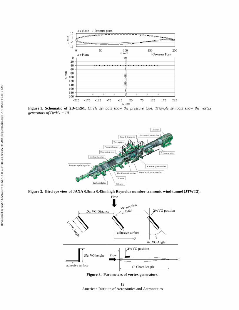
Figure 1 shows the airfoil of the 2D-CRM11. It was based on the airfoil of the 3D-CRM at η = 65% considering the sweepback angle of 31.5 degrees. The trailing edge was blunt. The chord and span length were 200 mm and 450 mm, respectively. Sweepback angle was zero. Main material of the model was stainless steel (HPM38).

The position of the pressure taps were shown as the circle symbols in Fig. 1. The 2D-CRM had three lines of the pressure taps on the upper surface and one line of those on the lower surface in the chord direction. The model also had a line of the pressure taps in the spanwise direction at x/C = 94 %. The total number of the pressure taps was 80.

In order to produce turbulent boundary layer, lines of disk roughness (Aeronautical Trip Dots, 3.1 mil Silver matte, CAD Cut inc.) were attached at x/C = 10 % on the upper and on the lower surface of the model. The height of the roughness was 0.0031 inch (79 µm) which was a little higher than the height of the estimation using the method in Ref. 19. The diameter and interval of the roughness disks were 0.05 inch and 0.1 inch, respectively.

2. Wind Tunnel

The experiments of the 2D-CRM were conducted in JAXA 0.8m x 0.45m high Reynolds number transonic wind tunnel (JTWT2)20, 21. Figure 2 presents the JTWT2. The JTWT2 is a high pressure blow down wind tunnel. The height and width of the test section were 800 mm and 450 mm, respectively. The top and bottom walls have slots to realize the transonic flow conditions.

The model was supported by both ends using supporters. There was no gap between the model and the side walls. To reduce the influence of the side walls, the boundary layer on the side walls was evacuated through the rigimesh plates upstream of the airfoil model. In this evacuation, an ejector system was used to increase the suction mass flow rate.

The design Mach number of the 3D-CRM was 0.85. Considering the effect of the sweepback angle of the 3D-CRM and the interference of the wind tunnel walls, the nominal Mach number before the wall interference correction was determined as 0.74. The averaged Mach number after the wall interference correction was 0.736. The nominal Reynolds number based on the chord length was 5 x 106. The Reynolds number of 5 x 106 was same as that of the NASA’s CRM experiments for forth drag prediction workshops (DPW-4)12. On this condition, duration time of the wind tunnel experiment was 60 s. The data for the six angles of attack were measured in one blow.

3. Vortex Generators

The effect of rectangular co-rotating VGs was investigated in this experiment. Figure 3 shows the shape and the parameters of VGs. Table 1 presents the experimental conditions for the 2D-CRM. Figure 4 shows the photos of the VGs and the 2D-CRM.

A line of the rectangular VGs was installed at Xv/C of 0.2. The heights of VGs Hv were 1.2 mm and 2.4 mm. The height of 1.2 mm was 1.5 times of the boundary layer thickness δ at the location of the VGs. The boundary layer thickness was estimated from CFD result. The deviation from the specified height of VGs was less than 0.05 mm. The VGs were made of stainless steel whose thickness was 0.1 mm. The lengths of VGs Lv were 4 times of the heights. The angle of VGs to the uniform flow direction Av was 20 degrees. The leading edge of all VGs turned to the left side. The intervals of adjacent VGs Dv were 10, 20, and 40 times of the VGs height. The relation between the VGs and pressure taps are shown in Fig. 1. The triangle symbols in Fig. 1 show the VGs location when the Dv/Hv was 10. The VGs on the center line (y = 0 mm) remained for all cases.

Generally, the size of VGs in the wind tunnel experiment is small since models are much smaller than the real wings. One of the difficulties of the VGs experiment is how to precisely attach the small VGs to the wing model and how to easily detach them in order to examine the many configurations of the line of VGs. The enough adhesive strength is also needed to withstand the aerodynamic force. In order to realize the wind tunnel experiment, we used a


3

Dow

nloa

ded

by N

ASA

LA

NG

LE

Y R

ESE

AR

CH

CE

NT

RE

on

Janu

ary

30, 2

018

| http

://ar

c.ai

aa.o

rg |

DO

I: 1

0.25

14/6

.201

5-12

37

jig and an acrylic-based adhesive (SKYLOCK RD-57G, VA-05, NIKKA SEIKO). The adhesive strength was 22.5 N/mm2. The VGs attached with the acrylic-based adhesive was easily detached with hot water. Details of the VGs installation are described in Ref. 6 and 7.

4. Measurement Techniques

The effect of the VGs was quantitatively investigated from the pressure distributions on the airfoil. The pressure from the 80 ports on the airfoil surface was measured with scanning-type pressure gauge. The uncertainty of the Cp was less than 0.02 except the region close to a shock wave and it was about 0.2 around the shock wave location. Pressure coefficients Cp, Mach number M, angle of attack AoA, and lift coefficient CL were corrected by Sawada’s method22, 23 to eliminate the influence of the interference of top and bottom wall. In order to use Sawada’s method, the static pressure on the top and bottom wall were measured with the static pressure rails. The pressure was measured at sampling rate of 1 ms. 20 points were sampled and averaged for the each pressure port. Since the response rate of the pressure measurement system was too slow, time resolved pressure data could not been obtained. However, the averaged pressure distributions clearly revealed the VGs effect as described in the section of results. In order to easily compare the VGs effect, the lift coefficients were calculated from the pressure distribution on the surface of the airfoil using the following equations. Here, i is the number of the pressure port. The order of the number i is as follows, leading edge – upper surface – trailing edge – lower surface – leading edge.

)sin()cos( AoACAoACC CNL −= (1)

( ) ( )[ ] ( ) ( )[ ]∑=

−+×++−

=in

ippN ixixiCiC

CC

1

112

1 (2)

( ) ( )[ ] ( ) ( )[ ]∑=

−+×++−

=in

ippC iziziCiC

CC

1

112

1 (3)

The uncertainty of the lift coefficient CL was less than 0.02 except the correction error of the wall interference.

As described in Ref. 23, Sawada’s correction method is not appropriate when the lift slop is not linear. Hence, strictly speaking, the corrected values under the shock wave oscillating condition have the correction error. However, the corrected values are shown in this paper in order to continuously show the data plot. The correction does not change the evaluation of the VGs effect in this experiment. The uncorrected values are suitably mentioned to clearly show the experimental conditions.

Oil flow visualization technique was used to investigate the flow pattern on the suction surface of the wing. The oil consisted of liquid paraffin, titanium dioxide as a dye, and a little oleic acid. The color of dye was white. The visualization data were recorded with a video camera mounted outside the test section on the top wall in the plenum chamber. The behavior of the oil pattern during each run was recorded continuously and specific scenes were captured from the movie data.

Color schlieren technique was used to visualize the shock waves and the expansion waves on the airfoil. The diameter of the concaved mirror was 300 mm. The light source was a xenon lamp. The schlieren images were recorded by a video camera. The recording was conducted both in the pressure measurement and in the oil flow visualization. Schlieren images were useful to monitor the flow and the model conditions.

B. Experiment of 3D-CRM 1. JAXA’s 80 % Scale NASA CRM

The NASA CRM consists of a contemporary supercritical transonic wing and a fuselage representative of a wide body commercial transport aircraft. The design Mach number and lift coefficient are 0.85 and 0.5, respectively, at a Reynolds number of 40 x 106. Details of the model are explained in Ref. 12 and on a web site13 prepared by NASA’s Langley Research Center (LaRC).

The JAXA CRM wind tunnel model (3D-CRM) is an 80 % scale of NASA’s wind tunnel model. Its size corresponds to 2.16 % of the assumed scale of the CRM. The model was sized for the JAXA 2m x 2m transonic wind tunnel (JTWT) such that the ratio of the model to the test section size is approximately the same as that for the National Transonic Facility (NTF). Reference area, reference chord, and span are 0.179014 m2, 0.15131 m, and 1.26927 m, respectively. Details of the model are explained in Ref. 17.


4

Dow

nloa

ded

by N

ASA

LA

NG

LE

Y R

ESE

AR

CH

CE

NT

RE

on

Janu

ary

30, 2

018

| http

://ar

c.ai

aa.o

rg |

DO

I: 1

0.25

14/6

.201

5-12

37

Figure 5 shows the photos of JAXA’s 80 % scale NASA CRM with VGs. The experimental conditions for the model were same as those in Ref. 17. The experiments were conducted in a configuration without the engine nacelles and the pylons. The model was supported by a dorsal sting. The WBT0 (wing/body/tail = 0 deg.) model configuration was selected. In order to produce a turbulent boundary layer on the model surface, disk roughness (Aeronautical Trip Dots, CAD Cut inc.) were attached on the main wings and the horizontal stabilizers at 10% chord length and on the fuselage at 1.5% of its length. The diameter and the distance of adjacent trip dot centers were 0.05 inch and 0.1 inch. The heights were calculated using the method in Ref. 19 with total pressure of 100 kPa. As mentioned below, the total pressure of the experimental conditions was 120 kPa. Hence the height of the trip dots was a little higher than the proper height. The height of the trip dots on the body, outer wings and horizontal stabilizers was 0.0031 inch. The heights on the inner-wings and the mid-wings were 0.0039 inch and 0.0035 inch, respectively.

2. Wind Tunnel

The experiments for the 3D-CRM were conducted in the JTWT. A bird-eye view drawing of the tunnel is shown in Fig. 6. The JTWT is a continuous pressurized wind tunnel. All tests were performed in the tunnel’s No. 4 cart which had porous walls. The size of the cart was 2 m in height, 2 m in width, and 4.13 m length. Nominal Mach number was 0.85. Corrected Mach number was a little lower than the nominal Mach number, 0.848. Total pressure and total temperature were 120 kPa and around 50 °C. The resulting nominal Reynolds number was 2.27 x 106. Although the Reynolds number of 2.27 x 106 was almost the half of the Reynolds number of 5 x 106 in the 2D-CRM experiments, as mentioned below, the experimental conditions of the ratio Hv/δ = 1.5 was fixed in the both experiments in order to make the similarity conditions.

3. Vortex Generators

Table 2 presents the experimental conditions of VGs for the 3D-CRM. The effect of rectangular co-rotating type VGs was investigated in this experiment. The design parameter for the VG geometry and setting was determined at a representative spanwise section on the outer wing where the shock induced flow separation starts as AoA increases. Height of all VGs for the 3D-CRM was 0.8 mm. The height of 0.8 mm was about 1.5 times of the boundary layer thickness δ at the representative spanwise location and about 2 times of δ near the wing tip. The thickness δ was estimated from a CFD result. The ratio Hv/δ of 1.5 is same as that in the case of Hv of 1.2 mm for the 2D-CRM experiments. The lengths of VGs Lv were 4 times of the height Hv. Hence the shape of the VGs for the 3D-CRM was same as that for the 2D-CRM.

The VGs attached on the wing were shown in Fig. 5. The rectangular VGs was installed at a line around Xv/C of 0.2. It was almost same as the location of that in the 2D-CRM experiments. The VGs were attached from η = 0.4 to the wing tip. The intervals of adjacent VGs Dv were 20, 40, and 80 times of the VGs height. The numbers of the VGs for each case were 23, 12, and 6 for each side of wing. The VGs on the η = 0.4 remained for all cases.

The direction of the VGs was toe-out which meant the leading edge of the VGs turned to the wing tip. Hence, from the view point of the downstream of the model, the direction of the vortex was clockwise on the right wing and counter clockwise on the left wing. The angle of VGs to the body axis was 32.6 degrees, which corresponds to the flow direction on the wing surface Av of 20 degrees at the representative spanwise location. Av = 20 degrees was same as the angle in the 2D-CRM experiments.

The VGs were made of stainless steel whose thickness was 0.1 mm. The deviation from the specified height of VGs was less than 0.05 mm. In the same way as the 2D-CRM experiments, we used jigs and an acrylic-based adhesive (SKYLOCK RD-57G, VA-05, NIKKA SEIKO). The experiment was conducted for the three cases decreasing the number of VGs. Unnecessary VGs were detached with hot water to investigate the larger interval case.

4. Measurement Techniques

Figure 7 shows the diagram of the measurement system. The measurement system was same as that in the previous research17. The balance used in the tests was the TB-M6-04 which was moment-type balance and the most frequently used in the JTWT. The precision of the drag measurement was less than 2 x 10-4 in this experiment. The force data and physical property of the uniform flow were corrected by the analyzing system of the Digital/Analog-Hybrid Wind Tunnel (DAHWIN)24-26 which made it possible to compare the results of CFD and wind tunnel test in real time. The influence of the support and the wing deformation were not eliminated by the corrections.

The model surface has 370 pressure taps: 325 taps on the left and right wings, 12 taps on the fuselage, and 33 taps on horizontal stabilizers. The wing taps are arranged on nine spanwise wing stations (η = 0.131, 0.201, 0.283,


5

Dow

nloa

ded

by N

ASA

LA

NG

LE

Y R

ESE

AR

CH

CE

NT

RE

on

Janu

ary

30, 2

018

| http

://ar

c.ai

aa.o

rg |

DO

I: 1

0.25

14/6

.201

5-12

37

0.397, 0.502, 0.603, 0.727, 0.846, and .950). The pressure taps are located mainly on the lower surface of the right wing and the upper surface of the left wing. The detailed arrangement of the pressure taps was shown in Ref. 17. To measure the surface pressure, PSI 64-port ESP modules with digital temperature compensation were installed in the model fuselage, and pressure data are acquired by a System 8400.

Oil flow visualization technique was used to investigate the flow pattern on the suction surface of the wing. The oil consisted of silicon oil and fluorescent pigment. Illuminating the ultraviolet light, the photos of the fluorescence from the oil were taken after the test.

II. Results

A. Results of 2D-CRM 1. Lift Coefficient

Hereafter, the physical values of the 2D-CRM experiments, M, Cp, CL, and AoA, are values after the wind tunnel wall corrections. The uncorrected values are expressed as the setting values.

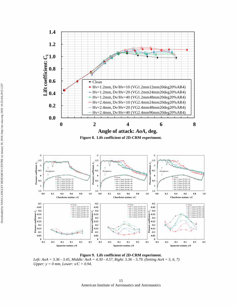
In the 2D-CRM experiments, lift coefficients were calculated from pressure coefficients Cp in order to evaluate the VGs effect quantitatively. Figure 8 shows the lift coefficient CL of the 2D-CRM. The vertical and horizontal axes show the CL and the angle of attack AoA. Closed circle symbols show the CL of the case without VGs (clean). Other closed and open symbols show the CL for the cases with VGs of Hv = 1.2 mm and 2.4mm, respectively.

In the clean case, the AoA to indicate the maximum CL was around 3.5 degrees. The CL of the clean continuously decreased after 3.5 degrees as the AoA increased. When the Dv/Hv was 10 (Red square symbols), the effect of the VGs clearly observed from the CL curves. The CL of the Dv/Hv = 10 were higher than that of the clean case at the AoA higher than 3.5 degrees. The effect of the VGs decreased as the Dv/Hv increased. The CL of Dv/Hv = 20 (Blue triangle) was smaller than those of Dv/Hv = 10. The effect of the VGs had little when the Dv/Hv was 40 (Green diamond).

2. Pressure Coefficient

Figure 9 presents the pressure coefficients Cp in the 2D-CRM experiments. The vertical axis is reversed to show the Cp in the manner that the upper line is the Cp profile on the suction surface. Upper figures show the Cp profiles on the center line. Lower figures show the Cp profile at x/C = 0.94 on the suction surface. In Fig. 9, the curves of the Cp at the same setting AoA are shown in the same graph. Because of the correction for the wall interference, the AoA of those cases were a little different from each other.

The characteristics of the Cp profiles on the buffet condition are the decrease of the Cp gradient around the shock wave location and the decrease of the Cp around the trailing edge. Since the instantaneous Cp profiles were averaged in the measurement, the gradient of the Cp around the shock wave location became low when the shock wave oscillated. Because of the flow separation, the Cp around the trailing edge was low on the buffet condition. Those characteristics were confirmed from the comparison between the schlieren movies and the Cp profiles.

At the AoA of 3.36 - 3.45, the shock wave didn’t oscillate in all cases. The gradient of the Cp around x/C = 0.6 was high and the profile of the Cp at x/C = 0.94 was almost flat and high. The difference between the clean and the VGs cases could be observed only in the region around VGs. The Cp of the VGs cases had peak around x/C = 0.2 because of the shock wave from the VGs.

At the AoA of 4.30 - 4.57, the Cp of the clean shows the buffet condition. The Cp gradient around x/C = 0.4 was low because of the shock wave oscillation. The Cp at x/C = 0.94 was not flat. The Cp around y/b = 0 decreased because of the flow separation. The VGs suppressed the shock wave oscillation and the flow separation when the Dv/Hv was 10. The Cp profiles of the Dv/Hv = 10 were different from that of the clean case. The gradient of Cp was still large around x/C = 0.5. The Cp at x/C = 0.94 was still almost flat and almost same as that at the AoA of 3.36 - 3.45. In the cases of Dv/Hv = 20, the effect of the VGs could be observed from the Cp at x/C = 0.94. The profiles of Dv/Hv = 20 were higher than that of the clean. The effect of VGs was small when the Dv/Hv = 40.

At the AoA of 5.36 – 5.79, the VGs of Dv/Hv = 10 and Hv = 1.2 mm still suppressed the buffet. The Cp gradient around x/C = 0.4 was high. The Cp at x/C = 0.94 was still almost flat and almost same as that at the AoA of 3.36 - 3.45 around the center line. The effect of VGs decreased as the Dv/Hv increased. In the case of Dv/Hv = 20 and 40, the profiles indicates that the shock wave oscillated on the suction surface.

3. Oil Flow Visualization

The oil flow images on the suction and left side of the airfoil are shown in Fig. 10. In Fig. 10, upper side is upstream and lower side is downstream. Oil flow images were obtained only for the clean case and the VGs case of


6

Dow

nloa

ded

by N

ASA

LA

NG

LE

Y R

ESE

AR

CH

CE

NT

RE

on

Janu

ary

30, 2

018

| http

://ar

c.ai

aa.o

rg |

DO

I: 1

0.25

14/6

.201

5-12

37

Hv = 1.2 mm. To show the location of the chord direction, lines and makers were painted on the model at x/C = 0.3, 0.4, 0.5, 0.6, 0.7, 0.8, and 0.9.

In the clean case, an oil line straightly spreads in the spanwise direction around x/C = 0.5 at AoA = 3.37. From the schlieren images and the pressure data, the straight oil line corresponds to the front of the separation bubble produced by the shock wave. At the AoA = 4.57, the straight oil line is still observed. But, the left side of the line is broken. At the AoA = 5.79, the straight oil line disappear. So the separation produced by the shock wave was oscillated.

When the Dv/Hv was 10, a characteristic wavy pattern spreads in the spanwise direction around x/C = 0.5. The wavy pattern was produced by the interaction between the shock wave and the VGs vortices. From AoA = 3.45 to 5.37, the wavy pattern could be observed. As the Dv/Hv increased, the wavy pattern became unclear. At AoA = 5.69, the wavy pattern of Dv/Hv = 40 almost disappears.

When the Dv/Hv was 10, the distance between the adjacent vortices was small. Hence the almost region were influenced by the vortices as shown in the wavy pattern of Dv/Hv = 10. When the Dv/Hv was 40, the straight lines spread in the spanwise direction between the wavy patterns. Those regions were not affected by the VGs vortices. As shown in Fig. 8, the effect of VGs was large at the Dv/Hv =10 and the effect was little at the Dv/Hv =40. When the VGs vortices do not fill the wing span at the shock wave location, the VGs do not suppress the shock wave oscillation for the 2D-CRM.

4. Schlieren Photographs

Figure 11 shows the schlieren photographs of the clean and the VGs case (Dv/Hv =10 and Hv = 1.2 mm). Because of the shock wave oscillation, the shock wave around x/C = 0.6 was not observed in the clean case at AoA = 4.57 and 5.79. In the VGs case, the shock wave was clearly observed at AoA = 4.38 although the shock wave was a little unclear at AoA = 5.37. The VGs suppressed the shock wave oscillation when the Dv/Hv was 10. Although the photos are not shown in Fig. 11, the VGs affected the shock wave oscillation on the schlieren movie even if the Dv/Hv was 40 at AoA = 4.53. The shock wave oscillated intermittently in the case.

B. Results of 3D-CRM 1. Aerodynamic Coefficients

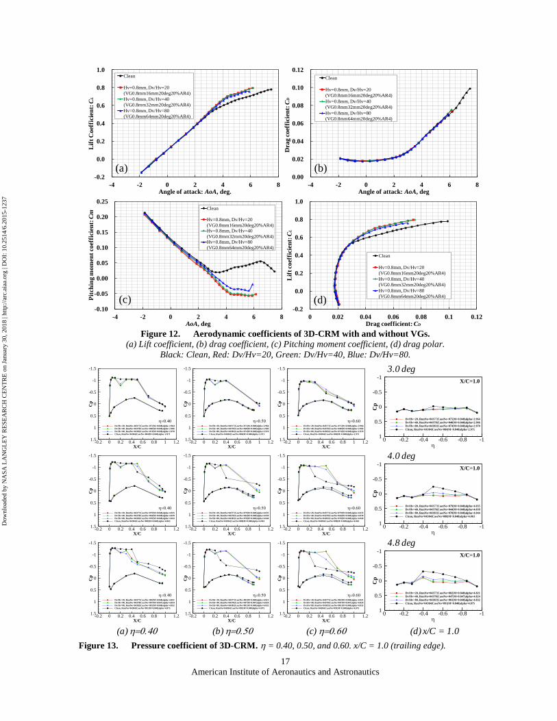
Hereafter, the physical values of the 3D-CRM experiments are values after the corrections of the DAHWIN24-26. Figure 12 presents lift, drag, and pitching moment coefficients and drag polar of the 3D-CRM. Circle symbols show the case without VGs (Clean). Square, diamond, and triangle symbols show the VGs cases of Dv/Hv = 20, 40, and 80, respectively. The height of the VGs was 0.8 mm in the 3D-CRM experiments. As mentioned above, the ratio of VG’s height Hv/δ was 1.5 which was same as that of Hv = 1.2mm in the 2D-CRM experiments.

For all VGs cases, the VGs improved the CL and the Cm at the high angle of attack. The CLs of VG cases are higher than that of the clean case. The Cm continuously decreased to about 4.4 degrees. It is important that the VGs for the 3D-CRM maintained their effect from Dv/Hv = 20 to 80. The effect of the VGs on 2D-CRM was little at Dv/Hv = 40. So the effect of VGs for the 3D-CRM was much larger than that for the 2D-CRM. The quantitative comparison of the 2D and 3D cases are described in section C.

The CD increased at low AoA because of the installation drag of the VGs. However, the CD decreased at high AoA since the separation was suppressed by the VGs. The details of the drag penalty are described in section D.

2. Pressure Coefficient

The pressure coefficient Cp on the wings shows the spatial information of the VGs effect. Figure 13 presents the Cp at η = 0.40, 0.50, and 0.60 and trailing edge x/C = 1.0. At AoA = 3.0, the Cp of the clean is a little lower than that of other cases at x/C = 1.0 and η = 0.50. The Cp indicates that the separation started around η = 0.50 of the trailing edge in the clean case. In the VGs cases, the separation was suppressed at the point.

The effect of VGs are clear at AoA = 4.0 and 4.8. The shock wave position was almost same as that at AoA = 3.0 in the VGs cases although the position moved upstream in the clean case. The Cp of the trailing edge decreased from η = -0.73 to -0.40 in the clean case. The Cp indicates that the separation area around trailing edge increased as the AoA increased in the clean case. In the VGs cases, the Cp was still higher than that in the clean case. The separation was suppressed by the VGs.

3. Oil Flow Visualization

The oil flow images on the suction and right wings are shown in Fig. 14 and Fig. 15. In both figures, upper side is upstream and lower side is downstream. The oil was painted on the wing surface from x/C = 0.2 for clean case and x/C = 0.3 for VGs cases to avoid the interaction between the oil and the disk roughness and between the oil and the


7

Dow

nloa

ded

by N

ASA

LA

NG

LE

Y R

ESE

AR

CH

CE

NT

RE

on

Janu

ary

30, 2

018

| http

://ar

c.ai

aa.o

rg |

DO

I: 1

0.25

14/6

.201

5-12

37

VGs. Hence, the upper boundary of the oil images is not the line of wing leading edge. White two direction arrows in the images of the clean case show the region where the Cp on the trailing edge decreased from that at the low AoA. So, the arrows roughly show the separation region around the trailing edge. In Fig. 14, the oil flow images of the VGs case of Dv/Hv = 40 are shown. Figure 15 shows the oil flow images of the all VGs cases at AoA = 4.0.

In Fig. 14, the large separation area appeared in the clean case at AoA = 4.0 and 4.8. The separation area mainly expanded to the outer board from AoA = 3.0 to 4.8. The effect of VGs is clear at these angles. In Fig. 14 and Fig. 15, the large separation area does not appear in the VGs cases. The separation area was segregated by the vortices produced by the VGs.

The trajectory of the vortices can be estimated from lines spreading to the chord direction. As shown in Fig. 15, the interval of the adjacent vortices were large when the Dv/Hv = 40 and 80. In these cases, the VG’s vortices did not fill the area of the wing at the shock wave location. In the 2D-CRM experiments, the effect of the VGs was little in such cases. However, the effect of the VGs was clear for the 3D-CRM even if the vortices did not fill the wing.

C. Comparison between 2D- and 3D-CRM Generally each VG produces installation drag on cruise conditions. Hence small number of VGs and large

interval of adjacent VGs are better for the drag penalty. The VGs on the 3D-CRM had a large effect at Dv/Hv = 80 although the VGs on the 2D-CRM had little at Dv/Hv = 40. The VGs effect on the 3D-CRM is more desirable than that on the 2D-CRM.

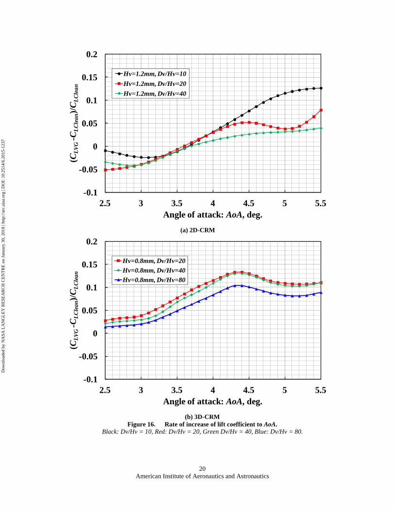
In order to quantitatively show the difference between 2D and 3D cases, a rate of increase of the lift coefficient CL (= (CLVG - CLClean) / CLClean) was calculated using the spline interpolation. Figure 16 (a) and (b) show the rate of the CL increase for the 2D-CRM and the 3D-CRM, respectively. Only the data of Hv/δ = 1.5 are shown for the comparison. The horizontal axis shows the AoA. The values of the low and the high AoA were doubtful because the spline interpolation was used and the number of the points was limited. Hence the low and the high AoA were eliminated from the Fig. 16.

In the 2D-CRM cases, the maximum rate of the CL increase is over ten percent at Dv/Hv = 10. The rate decreased rapidly as the Dv/Hv increased. The rate of Dv/Hv = 40 was less than half of the rate of Dv/Hv = 10. In the 3D-CRM cases, the rate was about ten percent for all cases. The maximum rate of Dv/Hv = 40 was almost same as that of Dv/Hv = 20. Although the rate of the Dv/Hv = 80 was a little smaller than other cases, the effect of the VGs was clear from Fig. 16 (b).

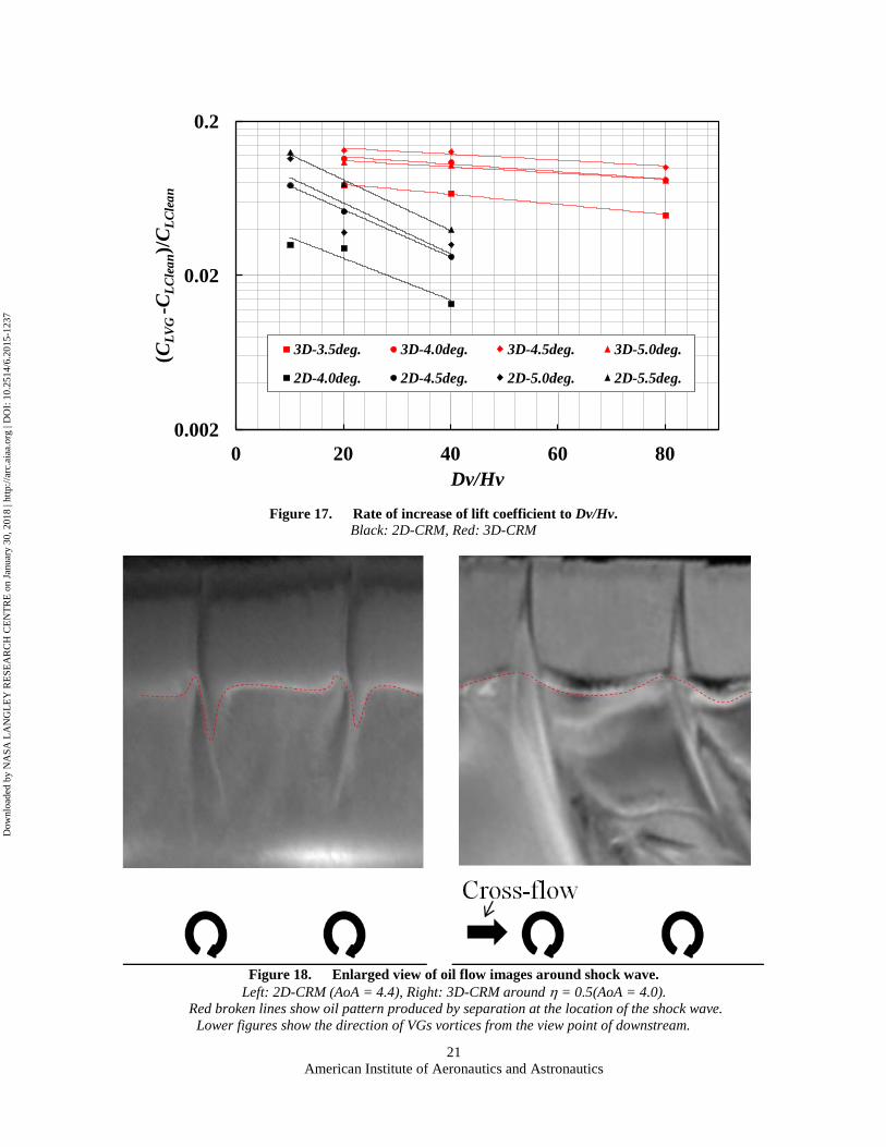
Figure 17 presents the rate of the CL increase to the Dv/Hv at the several AoA. The AoAs higher than the buffet conditions were selected in Fig. 17. The lines show exponential approximation curves. As the Dv/Hv increased, the rate rapidly decreased in the 2D cases. However, the rate maintained from the Dv/Hv = 20 to 80 in the 3D cases.

Figure 18 shows the enlarged view of the oil flow images of 2D- and 3D-CRM at Dv/Hv = 40. The images of 3D-CRM was around η = 0.5. In the 2D-CRM case, the VG’s vortex affected the limited region at the location of the shock wave. Although the oil line curved upstream and downstream on upwash and downwash side of the vortex, the straight oil line spread in the spanwise direction between the vortices. This straight line is similar to the oil line in the clean case and the straight line is the region where the influence of the vortex is little. In the 3D-CRM case, such a straight region could not be observed at the shock wave location. The all region was affected by the vortices and the oil lines mildly curved at the shock wave location. These oil patterns indicate that the influence of the VGs on the 3D-CRM was larger than that on the 2D-CRM.

The effect of the VGs was observed mainly on the mid span of the 3D-CRM. The primal difference between the mid span of the 3D-CRM and the 2D-CRM is sweepback angle. On the swept wings, cross-flow which is perpendicular to the axis of VG vortex appears because of the pressure gradient in the spanwise direction. Hence we considered the difference of the VGs effect between the 2D- and 3D-CRM was mainly caused by the cross-flow.

In the companion paper10, Ito et al. investigated the influence of the sweepback angle on the VGs effect using CFD. The influence of the sweepback angles was extracted to calculate flow fields on infinite two-dimensional swept wings. The results of the CFD agreed with the experimental results. The toe-out VGs on the swept wings was more effective than the VGs on the unswept wing because the cross-flow around the VG’s vortex enhanced the VGs effect. In addition, the surface stream lines of the CFD for unswept and swept wings were similar to the oil flow patterns of 2D- and 3D-CRM experiments shown in Fig. 18. From these results, we concluded that the effect of cross-flow was the main reason of the difference between the 2D- and 3D-CRM. The cross-flow is essentially important for the VGs effect.


8

Dow

nloa

ded

by N

ASA

LA

NG

LE

Y R

ESE

AR

CH

CE

NT

RE

on

Janu

ary

30, 2

018

| http

://ar

c.ai

aa.o

rg |

DO

I: 1

0.25

14/6

.201

5-12

37

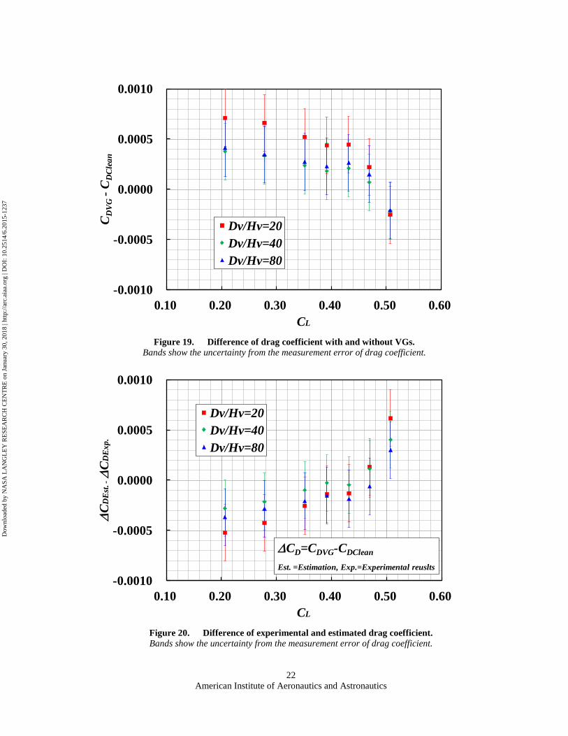
D. Penalty of VGs for 3D-CRM As shown in Fig. 12, the VGs increased the drag coefficient at low AoA. Figure 19 shows the difference between

the drag coefficient of the clean and the VGs cases (CDVG - CDClean). The horizontal axis shows the lift coefficient CL. Spline interpolation was used in order to obtain the difference CDVG - CDClean.

As shown in Fig. 19, the VGs increased the drag coefficient when the CL was less than 0.5. The drag increase of Dv/Hv = 20 was highest in the three cases. The drag coefficient was decreased by the VGs at the lift coefficient little larger than the design value of 0.5. The VGs suppressed the separation and the effect exceeded the installation drag of the VGs.

The installation drag of VGs (CDVG - CDClean) was estimated using the method in Ref. 27. The drag was estimated by the next equations. The several values in these equations can be obtained from the measurement values for the clean case and from the design parameters of VGs.

( )SSCFmC vgDfvgvgDvg ≅∆ (4)

90.F = (2) 52

2

2200124

M201M201600

2 .

TE

M..

TE

.vg

vg ..

UU

UU

.m

+

+

= ∞

−∞

∞

∞

(5)

( ) 21

72

22 11M70

M51

−+−= ∞

∞∞pC.

UU (6)

( )

21

72

2

22

1M70

M40252M

−

+

+=

∞

∞

pC.

.. (7)

vgLDfvg tanCC α= (8)

( ) ( )2020 vgLL vgCC αα == (9)

( ) 220 216706850031170 )AR(.AR..C

vgL −+==α (10)

LvHvAR 2

= (11)

LvHvSvg = (12)

Avvg =α (13) Here, ∆CDvg is the installation drag of isolated VG. The mvg is a magnification factor for isolated VG on a transonic-transport airplane. CDfvg is the drag coefficient of isolated VG on a flat plate wing. Svg and S are area of the isolated VG and reference area of the model, respectively. U and M are velocity and Mach number. Subscript TE and vg show the location of trailing edge and vortex generator for those values U and M.

Figure 20 shows the difference between the estimated installation drag ∆CDEst. and the experimental data ∆CDExp.. The ∆CDEst. is the total installation drag of VGs. If the estimation is appropriate, the values are close to zero. In Fig. 20, the difference was close to zero when the CL is larger than 0.35 and lower than 0.50. The estimation method is appropriate for the initial estimation of the installation drag of VGs.

III. Conclusions Aerodynamic characteristics of two- and three-dimensional NASA common research model (2D-CRM and 3D-

CRM) with co-rotating vortex generators (VGs) were investigated for several intervals of adjacent VGs Dv to clarify the influence of the three-dimensionality of the wings on the VGs effect.

In the 2D-CRM experiments, the nominal Mach number of the uniform flow was 0.74 considering the sweepback angle of the 3D-CRM. The nominal Reynolds number was 5 x 106. The base height of the VGs Hv was 1.5 times of the boundary layer thickness δ at the VGs location. The result of the pressure measurement and the flow


9

Dow

nloa

ded

by N

ASA

LA

NG

LE

Y R

ESE

AR

CH

CE

NT

RE

on

Janu

ary

30, 2

018

| http

://ar

c.ai

aa.o

rg |

DO

I: 1

0.25

14/6

.201

5-12

37

visualization showed the VGs on the 2D-CRM suppressed the buffet and increased the lift when the Dv/Hv was 10. However the VGs had little effect when the Dv/Hv was 40.

In the 3D-CRM experiments, the ratio of Hv/δ was determined as 1.5 in the same way as the 2D-CRM experiment. The direction of the VGs was toe-out which meant the leading edge of the VGs turned to the wing tip. The nominal Mach and Reynolds numbers were 0.85 and 2.27 x 106, respectively. The VGs on the 3D-CRM increased the lift and suppressed the separation on the wing even if the Dv/Hv was 80.

The comparison between the results of the 2D- and 3D-CRM showed that the effect of the VGs on the 3D-CRM was much larger than that on the 2D-CRM.The rate of the CL increase to the Dv/Hv rapidly decreased in the 2D-CRM cases as the Dv/Hv increased. However, the rate maintained from the Dv/Hv = 20 to 80 in the 3D-CRM cases. From the comparison between the experiments and the CFD results obtained by Ito et al. in the companion paper, we concluded that the difference between 2D- and 3D-CRM was mainly caused by the cross-flow due to the sweepback angles of the 3D-CRM wings. The cross-flow enhances the effect of the co-rotating toe-out VGs on the 3D-CRM wings. The effect of the cross-flow is essentially important for the estimation of the VGs effect.

The penalty of the VGs on the drag coefficient was also investigated in the 3D-CRM experiments. The drag of the 3D-CRM with VGs was higher than that in the clean case when the lift coefficient CL was less than 0.5. The drag of the 3D-CRM with VGs was lower than that in the clean case when the CL was higher than 0.5 because the VGs suppressed the separation and the effect exceeded the installation drag of the VGs. The estimation method proposed by Kusunose and Yu was appropriate for the initial estimation of installation drag of VGs.

Acknowledgments The experiments were conducted in JAXA wind tunnel technology center (WINTEC). The authors would like to

thank to the members of WINTEC.

References 1Pearcey, H. H., “Shock-Induced Separation and its Prevention,” in Lachmann, G. V. (Ed.), Boundary Layer and Flow

Control, Its Principles and Application, Vol. 2, Pergamon Press, Oxford, 1961. 2Pearcey, H. H. and Holder, D. W., “Examples of the Effects of Shock-Induced Boundary Layer Separation in Transonic

Flight,” ARC/R&M 3510, 1967. 3Engineering Science and Data Unit (ESDU) 93024, “Vortex Generators for Control of Shock-Induced Separation Part1:

Introduction and Aerodynamics,” 1993. 4Engineering Science and Data Unit (ESDU) 93025, “Vortex Generators for Control of Shock-Induced Separation Part2:

Guide to Use of Vane Vortex Generators,” 1994. 5Engineering Science and Data Unit (ESDU) 93026, “Vortex Generators for Control of Shock-Induced Separation Part3:

Example of Applications of Vortex Generators to Aircraft,” 1995. 6Koike, S., Sato, M., Kanda, H., Nakajima, T., Nakakita, K., Kusunose, K., Murayama, M., Ito, Y., and Yamamoto, K.,

“Experiment of Vortex Generators on NASA SC(2)-0518 Two Dimensional Wing for Buffet Reduction,” Proceedings of the 2013 Asia-Pacific International Symposium on Aerospace Technology, Takamatsu, Japan, Nov.20-22, 2013.

7Koike, S., Sato, M., Kanda, H., Nakajima, T., Nakakita, K., Kusunose, K., Murayama, M., Ito, Y., and Yamamoto, K., “Effect of Vortex Generators on Two-Dimensional Wings in Transonic Flows,” JAXA Research and Development Report, JAXA-RR-14-002, 2014 (in Japanese).

8Ito, Y., Murayama, M. and Yamamoto, K., “High-Quality Unstructured Hybrid Mesh Generation for Capturing Effects of Vortex Generators,” AIAA Paper 2013-0554, 51st AIAA Aerospace Sciences Meeting Including the New Horizons Forum and Aerospace Exposition, Grapevine, TX, January 2013, DOI: 10.2514/6.2013-554.

9Ito, Y., Murayama, M. and Yamamoto, K., “Efficient and Accurate Evaluation of Aircraft in Different Configurations with Automatic Local Remeshing,” AIAA Paper 2013-2711, 21st AIAA Computational Fluid Dynamics Conference, San Diego, CA, June 2013, DOI: 10.2514/6.2013-2711.

10Ito, Y., Yamamoto, K., Kusunose, K., Koike, S., Nakakita, K., Murayama, M., and Tanaka, K., “Effect of Vortex Generators on Transonic Swept Wings,” 53rd AIAA Aerospace Sciences Meeting, Kissimmee, FL, January 2015, to be presented.

11CRM.65.airfoil sections, http://commonresearchmodel.larc.nasa.gov/crm-65-airfoil-sections/ [cited 24 June 2014]. 12Vassberg, J., Dehaan, M., Rivers, M. and Wahls, R., “Development of a Common Research Model for Applied CFD

Validation Studies,” AIAA Paper 2008-6919, 26th AIAA Applied Aerodynamics Conference, Honolulu, HI, 2008, DOI: 10.2514/6.2008-6919.

13NASA Common Research Model, http://commonresearchmodel.larc.nasa.gov/ [cited 24 June 2014]. 14Ueno, M., Kohzai, M., Koga, S., Kato, H., Nakakita, K. and Sudani, N., “80% Scaled NASA Common Research Model

Wind Tunnel Test of JAXA at Relatively Low Reynolds Number,” AIAA Paper 2013-0493, 51st AIAA Aerospace Sciences Meeting Including the New Horizons Forum and Aerospace Exposition, Grapevine, TX, 2013, DOI: 10.2514/6.2013-493.


10

Dow

nloa

ded

by N

ASA

LA

NG

LE

Y R

ESE

AR

CH

CE

NT

RE

on

Janu

ary

30, 2

018

| http

://ar

c.ai

aa.o

rg |

DO

I: 1

0.25

14/6

.201

5-12

37

15Koga, S., Kohzai, M., Ueno, M., Nakakita, K. and Sudani, N., “Analysis of NASA Common Research Model Dynamic Data in JAXA Wind Tunnel Tests,” AIAA Paper 2013-0495, 51st AIAA Aerospace Sciences Meeting Including the New Horizons Forum and Aerospace Exposition, Grapevine, TX, 2013, DOI: 10.2514/6.2013-495.

16Kohzai, M., Ueno, M., Koga, S. and Sudani, N., “Wall and Support Interference Corrections of NASA Common Research Model Wind Tunnel Tests in JAXA,” AIAA Paper 2013-0963, 51st AIAA Aerospace Sciences Meeting Including the New Horizons Forum and Aerospace Exposition, Grapevine, TX, 2013, DOI: 10.2514/6.2013-963.

17Ueno, M., Kohzai, T., and Koga, S., “Transonic Wind Tunnel Test of the NASA CRM (Volum1),” JAXA Research and Development Memorandum, JAXA-RM-13-017E, 2014.

18Harris, C. D., “NASA Supercritical Airfoils—a Matrix of Family-Related Airfoils,” NASA Technical Paper 2969, 1990. 19Braslow, A. L., and Knox, E. C., “Simplified Method for Determination of Critical Height of Distributed Roughness

Particles for Boundary-Layer Transition at Mach Numbers from 0 to 5,” NACA-TN-4363, 1958. 20Second Aerodynamics Division Staff “Construction and Performance of NAL Two-Dimensional Transonic Wind Tunnel,”

National Aerospace Lab., Rept. TR-647T, 1982 (in Japanese). 21Two-Dimensional Transonic Wind Tunnel Staff “Revitalization of NAL Two-Dimensional Transonic Wind Tunnel,”

National Aerospace Lab., Rept. TM-744, 1999 (in Japanese). 22Sawada, H., “A Genearal Correction Method of the Interference in 2-Dimensional Wind Tunnels with Ventilated Walls,”

Transactions of the Japan Society for Aeronautical and Space Sciences, Vol. 21, No.52, 1978, pp. 57-68. 23Sawada, H., Sakakibara, S., Sato, M., and Kanda, H., “Wall Interference Estimation of the NAL’s Two-Dimensional Wind

Tunnel,” National Aerospace Lab., Rept. TR-829, 1984 (in Japanese). 24Kawamoto, I., Oguni, Y., Nakamura, S., and Hosoe, N., “Corrections to the Experimental Data of the NAL-TWT –Mach

Number and Buoyancy Corrections,” Proceedings of 30th fluid dynamics conference, 1998, pp. 365-368 (in Japanese). 25Kohzai, M., Ueno, M., Shiohara, T., Komatsu, Y., Karasawa, T., Koike, A., Sudani, N., Ganaha, Y., Kon, N., Haraguchi, T.,

and Nakamura, A., ”Calibration of the test section Mach number in the JAXA 2m x 2m Transonic Wind Tunnel,” Proceedings of the Wind Tunnel Technology Association 77th meeting, JAXA Special Publication, JAXA-SP-06-026, 2007, pp. 6-14 (in Japanese).

26Hidaka, A., Kuchiishi, S., Koike, A., Kohzai, M., and Morita, Y., “Wall Interference Correction by the Panel Method for the JAXA 2m x 2m Transonic Wind Tunnel,” JAXA Research and Development Report, JAXA-RR-07-033, 2007 (in Japanese).

27Kusunose, K. and Yu, N. J., “Vortex Generator Installation Drag on an Airplane near Its Cruise Condition,” Journal of Aircraft, Vol. 40, No. 6, 2003, pp. 1145-1151, DOI: 10.2514/2.7203.


11

Dow

nloa

ded

by N

ASA

LA

NG

LE

Y R

ESE

AR

CH

CE

NT

RE

on

Janu

ary

30, 2

018

| http

://ar

c.ai

aa.o

rg |

DO

I: 1

0.25

14/6

.201

5-12

37

020406080

100120140160180200

-225 -175 -125 -75 -25 25 75 125 175 225

Pressure Portsx-y Plane

x, m

m

y, mm

x, mm

z, m

m

-15-55

15

0 50 100 150 200

Pressure portsx-z plane

Figure 1. Schematic of 2D-CRM. Circle symbols show the pressure taps. Triangle symbols show the vortex generators of Dv/Hv = 10.

Pressure regulating valve

Settling chamber

Contraction cone

Plenum chamber

Test section

Sting & Strut unit

Diffuser

The second throat valve

Perforated plate

Schlieren glass window

Boundary layer suction ductFlexible nozzle section

Screens

SilencerPerforated plate

Figure 2. Bird eye view of JAXA 0.8m x 0.45m high Reynolds number transonic wind tunnel (JTWT2).

Flow

adhesive surface

Dv: VG Distance

Av: VG Angle

Xv: VG position

y

Hv: VG height

adhesive surface

Xv: VG position

C: Chord length

xFlow

Figure 3. Parameters of vortex generators.


12

Dow

nloa

ded

by N

ASA

LA

NG

LE

Y R

ESE

AR

CH

CE

NT

RE

on

Janu

ary

30, 2

018

| http

://ar

c.ai

aa.o

rg |

DO

I: 1

0.25

14/6

.201

5-12

37

Figure 4. Photos of 2D-CRM with vortex generators.

Table 1. Parameters of 2D-CRM experiments.

Experimental conditions Hv , mm Hv/δ ∗1 Dv , mm Dv/Hv Av , deg Xv/C Lv/Hv (AR)VG1.2mm12mm20deg20%AR4 1.2 1.5 12 10 20 0.2 4VG1.2mm24mm20deg20%AR4 1.2 1.5 24 20 20 0.2 4VG1.2mm48mm20deg20%AR4 1.2 1.5 48 40 20 0.2 4VG2.4mm24mm20deg20%AR4 2.4 3.0 24 10 20 0.2 4VG2.4mm48mm20deg20%AR4 2.4 3.0 48 20 20 0.2 4VG2.4mm96mm20deg20%AR4 2.4 3.0 96 40 20 0.2 4

*1 δ is boundary layer thickness estimated from CFD results.

Figure 5. Photos of JAXA’s 80% scale NASA CRM (3D-CRM) with vortex generators.


13

Dow

nloa

ded

by N

ASA

LA

NG

LE

Y R

ESE

AR

CH

CE

NT

RE

on

Janu

ary

30, 2

018

| http

://ar

c.ai

aa.o

rg |

DO

I: 1

0.25

14/6

.201

5-12

37

Figure 6. Bird eye view of JAXA 2m x 2m transonic wind tunnel (JTWT).

Table 2. Parameters of 3D-CRM experiments.

Experimental conditions Hv , mm Hv/δ Dv , mm Dv/Hv Av , deg*2 VG direction Xv/C *3 Lv/Hv (AR) η N VG*4

VG0.8mm16mm20deg20%AR4 0.8 1.5 16 20 20 Toe-out about 0.2 4 0.4 - wing tip 23VG0.8mm32mm20deg20%AR4 0.8 1.5 32 40 20 Toe-out about 0.2 4 0.4 - wing tip 12VG0.8mm64mm20deg20%AR4 0.8 1.5 64 80 20 Toe-out about 0.2 4 0.4 - wing tip 6

*2 Av shows VGs angle to the flow direction on a main wing. Angle to the body axis is 32.6 degrees.*3Xv/C is depend on the η. Xv/C in the table shows the location on the outboard.*4 N VG is the number of VGs on a half wing.

*1 δ is boundary layer thickness estimated from CFD results.

Figure 7. Measurement system of JAXA’s 80% scale NASA CRM (3D-CRM).


14

Dow

nloa

ded

by N

ASA

LA

NG

LE

Y R

ESE

AR

CH

CE

NT

RE

on

Janu

ary

30, 2

018

| http

://ar

c.ai

aa.o

rg |

DO

I: 1

0.25

14/6

.201

5-12

37

0.0

0.2

0.4

0.6

0.8

1.0

1.2

1.4

0 2 4 6 8

Lift

coef

ficie

nt:C

L

Angle of attack: AoA, deg.

CleanHv=1.2mm, Dv/Hv=10 (VG1.2mm12mm20deg20%AR4)Hv=1.2mm, Dv/Hv=20 (VG1.2mm24mm20deg20%AR4)Hv=1.2mm, Dv/Hv=40 (VG1.2mm48mm20deg20%AR4)Hv=2.4mm, Dv/Hv=10 (VG2.4mm24mm20deg20%AR4)Hv=2.4mm, Dv/Hv=20 (VG2.4mm48mm20deg20%AR4)Hv=2.4mm, Dv/Hv=40 (VG2.4mm96mm20deg20%AR4)

Figure 8. Lift coefficient of 2D-CRM experiment.

-2

-1.5

-1

-0.5

0

0.5

1

1.50.0 0.2 0.4 0.6 0.8 1.0

Pres

sure

coe

ffic

ient

: Cp

Chordwise station: x/C

CleanHv=1.2mm, Dv/Hv=10Hv=1.2mm, Dv/Hv=20Hv=1.2mm, Dv/Hv=40Hv=2.4mm, Dv/Hv=10Hv=2.4mm, Dv/Hv=20Hv=2.4mm, Dv/Hv=40

Roughness

-2

-1.5

-1

-0.5

0

0.5

1

1.50.0 0.2 0.4 0.6 0.8 1.0

Pres

sure

coe

ffic

ient

: Cp



Roughness

-2

-1.5

-1

-0.5

0

0.5

1

1.50.0 0.2 0.4 0.6 0.8 1.0

Pres

sure

coe

ffic

ient

: Cp



Roughness

-0.5-0.45

-0.4-0.35

-0.3-0.25

-0.2-0.15

-0.1-0.05

0-0.5 -0.3 -0.1 0.1 0.3 0.5

Pres

sure

coe

ffic

ient

: Cp

Spanwise station: y/b


-0.5-0.45

-0.4-0.35

-0.3-0.25

-0.2-0.15

-0.1-0.05

0-0.5 -0.3 -0.1 0.1 0.3 0.5

Pres

sure

coe

ffic

ient

: Cp



-0.5-0.45

-0.4-0.35

-0.3-0.25

-0.2-0.15

-0.1-0.05

0-0.5 -0.3 -0.1 0.1 0.3 0.5

Pres

sure

coe

ffic

ient

: Cp



Figure 9. Lift coefficient of 2D-CRM experiment. Left: AoA = 3.36 - 3.45, Middle: AoA = 4.30 - 4.57, Right: 5.36 – 5.79. (Setting AoA = 5, 6, 7) Upper: y = 0 mm, Lower: x/C = 0.94.


15

Dow

nloa

ded

by N

ASA

LA

NG

LE

Y R

ESE

AR

CH

CE

NT

RE

on

Janu

ary

30, 2

018

| http

://ar

c.ai

aa.o

rg |

DO

I: 1

0.25

14/6

.201

5-12

37

Figure 10. Oil flow images of 2D-CRM experiment. (a) Clean, (b) Hv=1.2mm, Dv/Hv=10, (c) Hv=1.2mm, Dv/Hv=20, (d) Hv=1.2mm, Dv/Hv=40. Setting AoA = 5, 6, 7. Caption show the corrected AoA.

Figure 11. Schlieren photographs of 2D-CRM.

Upper: Clean, Lower: Hv = 1.2mm, Dv/Hv = 10, Setting AoA = 5, 6, 7. Captions show the corrected AoA.


16

Dow

nloa

ded

by N

ASA

LA

NG

LE

Y R

ESE

AR

CH

CE

NT

RE

on

Janu

ary

30, 2

018

| http

://ar

c.ai

aa.o

rg |

DO

I: 1

0.25

14/6

.201

5-12

37

-0.2

0.0

0.2

0.4

0.6

0.8

1.0

-4 -2 0 2 4 6 8

Lift

Coe

ffic

ient

: CL


Clean

Hv=0.8mm, Dv/Hv=20 (VG0.8mm16mm20deg20%AR4)Hv=0.8mm, Dv/Hv=40 (VG0.8mm32mm20deg20%AR4)Hv=0.8mm, Dv/Hv=80 (VG0.8mm64mm20deg20%AR4)

(a)

-0.10

-0.05

0.00

0.05

0.10

0.15

0.20

0.25

-4 -2 0 2 4 6 8

Pitc

hing

mom

ent c

oeff

icie

nt: C

m

AoA, deg

Clean


(c)

0.00

0.02

0.04

0.06

0.08

0.10

0.12

-4 -2 0 2 4 6 8

Dra

g co

effic

ient

: CD

Angle of attack: AoA, deg

Clean


(b)

-0.2

0.0

0.2

0.4

0.6

0.8

1.0

0 0.02 0.04 0.06 0.08 0.1 0.12

Lift

coef

ficie

nt: C

L

Drag coefficient: CD

Clean

Hv=0.8mm, Dv/Hv=20 (VG0.8mm16mm20deg20%AR4)Hv=0.8mm, Dv/Hv=40 (VG0.8mm32mm20deg20%AR4)Hv=0.8mm, Dv/Hv=80 (VG0.8mm64mm20deg20%AR4)(d)

Figure 12. Aerodynamic coefficients of 3D-CRM with and without VGs.

(a) Lift coefficient, (b) drag coefficient, (c) Pitching moment coefficient, (d) drag polar. Black: Clean, Red: Dv/Hv=20, Green: Dv/Hv=40, Blue: Dv/Hv=80.

X/C

Cp

-0.2 0 0.2 0.4 0.6 0.8 1 1.2

-1.5

-1

-0.5

0

0.5

1

1.5

Dv/Hv=20, RunNo=04377|CaseNo=075|M=0.848|alpha=2.964Dv/Hv=40, RunNo=04378|CaseNo=040|M=0.848|alpha=2.966Dv/Hv=80, RunNo=04383|CaseNo=074|M=0.848|alpha=2.970Clean, RunNo=04384|CaseNo=084|M=0.848|alpha=2.971

η=0.50

X/C

Cp

-0.2 0 0.2 0.4 0.6 0.8 1 1.2

-1.5

-1

-0.5

0

0.5

1

1.5


η=0.40

η

Cp

-1-0.8-0.6-0.4-0.20

-1

-0.5

0

0.5

1


X/C=1.0

X/C

Cp

-0.2 0 0.2 0.4 0.6 0.8 1 1.2

-1.5

-1

-0.5

0

0.5

1

1.5


η=0.60

X/C

Cp

-0.2 0 0.2 0.4 0.6 0.8 1 1.2

-1.5

-1

-0.5

0

0.5

1

1.5


η=0.40

X/C

Cp

-0.2 0 0.2 0.4 0.6 0.8 1 1.2

-1.5

-1

-0.5

0

0.5

1

1.5


η=0.50

η

Cp

-1-0.8-0.6-0.4-0.20

-1

-0.5

0

0.5

1


X/C=1.0

X/C

Cp

-0.2 0 0.2 0.4 0.6 0.8 1 1.2

-1.5

-1

-0.5

0

0.5

1

1.5


η=0.60

X/C

Cp

-0.2 0 0.2 0.4 0.6 0.8 1 1.2

-1.5

-1

-0.5

0

0.5

1

1.5


η=0.60

X/C

Cp

-0.2 0 0.2 0.4 0.6 0.8 1 1.2

-1.5

-1

-0.5

0

0.5

1

1.5


η=0.40

X/C

Cp

-0.2 0 0.2 0.4 0.6 0.8 1 1.2

-1.5

-1

-0.5

0

0.5

1

1.5


η=0.50

η

Cp

-1-0.8-0.6-0.4-0.20

-1

-0.5

0

0.5

1


X/C=1.0

(a) η=0.40 (b) η=0.50 (c) η=0.60 (d) x/C = 1.0

3.0 deg

4.0 deg

4.8 deg

Figure 13. Pressure coefficient of 3D-CRM. η = 0.40, 0.50, and 0.60. x/C = 1.0 (trailing edge).


17

Dow

nloa

ded

by N

ASA

LA

NG

LE

Y R

ESE

AR

CH

CE

NT

RE

on

Janu

ary

30, 2

018

| http

://ar

c.ai

aa.o

rg |

DO

I: 1

0.25

14/6

.201

5-12

37

Figure 14. Oil flow images of 3D-CRM.

Upper: AoA= 3.0, Middle: AoA = 4.0, Lower: AoA = 4.8 Left: Clean, Right: Dv/Hv=40


18

Dow

nloa

ded

by N

ASA

LA

NG

LE

Y R

ESE

AR

CH

CE

NT

RE

on

Janu

ary

30, 2

018

| http

://ar

c.ai

aa.o

rg |

DO

I: 1

0.25

14/6

.201

5-12

37

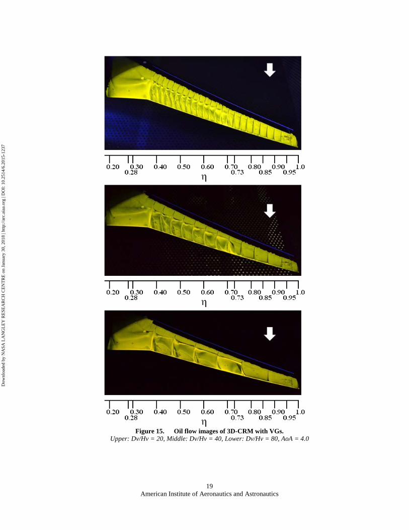
Figure 15. Oil flow images of 3D-CRM with VGs.

Upper: Dv/Hv = 20, Middle: Dv/Hv = 40, Lower: Dv/Hv = 80, AoA = 4.0


19

Dow

nloa

ded

by N

ASA

LA

NG

LE

Y R

ESE

AR

CH

CE

NT

RE

on

Janu

ary

30, 2

018

| http

://ar

c.ai

aa.o

rg |

DO

I: 1

0.25

14/6

.201

5-12

37

-0.1

-0.05

0

0.05

0.1

0.15

0.2

2.5 3 3.5 4 4.5 5 5.5

(CLV

G -C

LCle

an)/C

LCle

an


Hv=1.2mm, Dv/Hv=10Hv=1.2mm, Dv/Hv=20Hv=1.2mm, Dv/Hv=40

(a) 2D-CRM

-0.1

-0.05

0

0.05

0.1

0.15

0.2

2.5 3 3.5 4 4.5 5 5.5

(CLV

G -C

LCle

an)/C

LCle

an


Hv=0.8mm, Dv/Hv=20Hv=0.8mm, Dv/Hv=40Hv=0.8mm, Dv/Hv=80

(b) 3D-CRM

Figure 16. Rate of increase of lift coefficient to AoA. Black: Dv/Hv = 10, Red: Dv/Hv = 20, Green Dv/Hv = 40, Blue: Dv/Hv = 80.


20

Dow

nloa

ded

by N

ASA

LA

NG

LE

Y R

ESE

AR

CH

CE

NT

RE

on

Janu

ary

30, 2

018

| http

://ar

c.ai

aa.o

rg |

DO

I: 1

0.25

14/6

.201

5-12

37

0.002

0.02

0.2

0 20 40 60 80

(CLV

G -C

LCle

an)/C

LCle

an

Dv/Hv

3D-3.5deg. 3D-4.0deg. 3D-4.5deg. 3D-5.0deg.

2D-4.0deg. 2D-4.5deg. 2D-5.0deg. 2D-5.5deg.

Figure 17. Rate of increase of lift coefficient to Dv/Hv.

Black: 2D-CRM, Red: 3D-CRM

Figure 18. Enlarged view of oil flow images around shock wave.

Left: 2D-CRM (AoA = 4.4), Right: 3D-CRM around η = 0.5(AoA = 4.0). Red broken lines show oil pattern produced by separation at the location of the shock wave.

Lower figures show the direction of VGs vortices from the view point of downstream.


21

Dow

nloa

ded

by N

ASA

LA

NG

LE

Y R

ESE

AR

CH

CE

NT

RE

on

Janu

ary

30, 2

018

| http

://ar

c.ai

aa.o

rg |

DO

I: 1

0.25

14/6

.201

5-12

37

-0.0010

-0.0005

0.0000

0.0005

0.0010

0.10 0.20 0.30 0.40 0.50 0.60

C DV

G -

C DC

lean

CL

Dv/Hv=20Dv/Hv=40Dv/Hv=80

Figure 19. Difference of drag coefficient with and without VGs.

Bands show the uncertainty from the measurement error of drag coefficient.

-0.0010

-0.0005

0.0000

0.0005

0.0010

0.10 0.20 0.30 0.40 0.50 0.60

∆CD

Est

. -∆

CDE

xp.

CL

Dv/Hv=20Dv/Hv=40Dv/Hv=80

∆CD=CDVG-CDClean

Est. =Estimation, Exp.=Experimental reuslts

Figure 20. Difference of experimental and estimated drag coefficient. Bands show the uncertainty from the measurement error of drag coefficient.


22

Dow

nloa

ded

by N

ASA

LA

NG

LE

Y R

ESE

AR

CH

CE

NT

RE

on

Janu

ary

30, 2

018

| http

://ar

c.ai

aa.o

rg |

DO

I: 1

0.25

14/6

.201

5-12

37

Experimental Investigation of Vortex Generator Effect on ... · = reference area . S ... x =...

Documents

Transcript of Experimental Investigation of Vortex Generator Effect on ... · = reference area . S ... x =...