EXPERIMENTAL DESIGN AND ROBUST PARAMETER DESIGN IN ...
186
The Pennsylvania State University The Graduate School College of Engineering EXPERIMENTAL DESIGN AND ROBUST PARAMETER DESIGN IN MULTIPLE STAGE MANUFACTURING FOR NANO-ENABLED SURGICAL INSTRUMENTS A Dissertation in Industrial Engineering and Operations Research by Chumpol Yuangyai 2009 Chumpol Yuangyai Submitted in Partial Fulfillment of the Requirements for the Degree of Doctor of Philosophy December 2009
Transcript of EXPERIMENTAL DESIGN AND ROBUST PARAMETER DESIGN IN ...
The Pennsylvania State University
The Graduate School
College of Engineering
EXPERIMENTAL DESIGN AND ROBUST PARAMETER DESIGN
IN MULTIPLE STAGE MANUFACTURING FOR NANO-ENABLED SURGICAL
INSTRUMENTS
A Dissertation in
Industrial Engineering and Operations Research
by
Chumpol Yuangyai
2009 Chumpol Yuangyai
Submitted in Partial Fulfillment
of the Requirements
for the Degree of
Doctor of Philosophy
December 2009

The dissertation of Chumpol Yuangyai was reviewed and approved* by the
following:
Harriet Black Nembhard
Associate Professor of Industrial Engineering and
Bashore Career Professor
Dissertation Advisor
Chair of Committee
Sanjay Joshi
Professor of Industrial Engineering
Dennis K. J. Lin
Distinguished Professor of Statistics and Supply Chain Management
Affiliate Professor of Industrial Engineering
Mary Frecker
Professor of Mechanical Engineering
Paul Griffin
Professor of Industrial Engineering
Peter and Angela Dal Pezzo Head of Industrial and Manufacturing Engineering
*Signatures are on file in the Graduate School

iii
Abstract
The advent of rapid and exciting scientific advances in nanotechnology and
nanomanufacturing allows scientists and engineers to create new and sophisticated
products. However, the quality and yield of these products is still limited. Based on a
review of the literature, we recognized several opportunities to use statistically-based
design of experiments (DOE) and robust parameter design (RPD) in this field.
More specifically, along with a team of Penn State researchers, we have been
advancing a new multi-functional forceps-scissors (FS) instrument for minimally
invasive surgery (MIS). The lost mold rapid infiltration forming (LMRIF) process is
being developed to fabricate the tiny tool. There are many technical and quality issues
that need to be overcome. Furthermore, when this novel process is established in the
laboratory and ready to transition to full scale manufacturing, its continuing
repeatability and reproducibility must be assured.
In the experimentation to develop and refine the LMRIF process, there are
restrictions on the randomization, by which we mean that the allocation of the
experimental material and the order in which the individual trials of the experiment are
to be performed are not randomly determined because certain process variables are
‚hard to change" or ‚expensive to change" due to the nature of the multiple stages that
are involved in the process. Randomization, however, is one of the key principles in
DOE. If the principle of randomization is violated, and the typical approach to data
analysis is still employed, serious misinterpretation of the results may occur. This will

iv
lead to delays and/or diminished reliability in new product development. While there is
a rich history and body of literature on DOE, there is a gap between the literature and
the problem that we propose to address.
In this research, we develop the multistage fractional factorial split-plot
(MSFFSP) design with the combination of split-plot and split-block structure. Some
properties are derived and its application is demonstrated in the green-bar yield
improvement of the LMRIF process. Furthermore, we develop a framework of DOE and
RPD to expedite the transition of micro- and nano-scale technologies into robust
products that can be produced with minimum variability and defects.
To maximize the information obtained from the MSFFSP design, we extend an
algorithm from Bingham and Sitter (1999, 2001) to determine the optimal design under
two general criteria: maximum resolution and minimum aberration. The algorithm is
coded in MATLAB and is used to construct design catalogs for three and four stage
experiments. An application to the LMRIF process is explored.
In order to reduce the variability in the LMRIF process when it is transferred
from the laboratory scale to full scale manufacturing, we integrate the MSFFSP design
with the RPD concept. We focus on addressing multiple stages and multiple sets of noise
factors in this integration, which is convenient for the LMRIF process. A foundation for
using the concept is laid out and an optimal design catalog based on modified minimum
aberration criteria for the variation reduction is provided for two-stage experiments with
two sets of controllable factors and one set of noise factors. A computer code in

v
MATLAB is also constructed for this purpose, and it can be used for larger
experimentation. An application of the model is also explored for the improvement of
the fired FS yield of the LMRIF process.
The MSFFSP design and its integration with the RPD concept result in a more
rapid understanding of the interaction among process conditions, product
characteristics, and product reproducibility under constrained resources. This will not
only advance the field of quality engineering in nanomanufacturing, but also has
potential applications for other types of manufacturing.

vi
Table of Contents
List of Figures ................................................................................................................................ x
List of Tables ................................................................................................................................ xii
Acknowledgements .................................................................................................................... xv
Chapter 1. Introduction ......................................................................................................... 1
1.1 Background ................................................................................................................ 1
1.2 Motivation .................................................................................................................. 2
1.2.1 Quality Engineering Tools in Nanotechnology ............................................ 2
1.2.2 Devices for Minimally Invasive Surgery ....................................................... 4
1.3 Lost Mold Rapid Infiltration Forming Process...................................................... 9
1.4 Research Topics ....................................................................................................... 13
1.4.1 Multistage Design of Experiment ................................................................. 13
1.4.2 Robust Parameter Design for Multistage Experimentation ...................... 14
1.5 Research Objectives ................................................................................................. 15
1.6 Research Contributions .......................................................................................... 16
1.7 Outline of the Dissertation ..................................................................................... 17
Chapter 2. Literature Review.............................................................................................. 19
2.1 Introduction to Design of Experiments ................................................................ 20
2.2 OFAT: The Predominant Method Used in Practice ............................................ 22
2.3 Traditional Methods used in Research and Development ................................ 26
2.3.1 Completely Randomized Design (CRD) ...................................................... 27
vii
2.3.2 Two-level Factorial Design ............................................................................ 29
2.3.3 Response Surface Methodology (RSM) ........................................................ 31
2.3.4 Taguchi’s Method ............................................................................................ 34
2.4 Opportunities for Improvement in Experimentation ......................................... 35
2.5 Modern DOE Methods Appropriate for Nanotechnology and
Nanomanufacturing ................................................................................................ 37
2.5.1 Split-Plot Design and its Variants ................................................................. 38
2.5.2 Multistage Split-Plot Design .......................................................................... 41
2.5.3 Repeated Measures ......................................................................................... 42
2.5.4 Saturated and Supersaturated Design.......................................................... 43
2.5.5 Mixture Design ................................................................................................ 45
2.5.6 Computer Deterministic Experiments ......................................................... 46
2.5.7 Computer Generated Design: Alphabetical Optimal Design ................... 46
2.6 Summary of Nanotechnology Articles that use Statistical Experimentation .. 48
2.7 Remarks .................................................................................................................... 61
Chapter 3. Multistage Fractional Factorial Split-Plot Designs ....................................... 62
3.1 Yield Improvement for LMRIF Process ................................................................ 62
3.2 Choice of Design ...................................................................................................... 64
3.3 MSFFSP Design with Three-stage Experimentation .......................................... 66
3.4 Linear Model of the Three stage Split-Plot Design and Its Derivation ............ 73
3.4.1 Derivation ......................................................................................................... 73

viii
3.4.2 Analysis of the MSFFSP Design .................................................................... 83
3.5 MSFFSP Design Implementation for LMRIF process ......................................... 89
3.5.1 Implementation ............................................................................................... 89
3.5.2 Results, Analysis and Discussion .................................................................. 91
3.6 Remarks .................................................................................................................... 95
Chapter 4. Optimal Multistage Fractional Factorial Split-Plot Design ......................... 97
4.1 Optimal MSFFSP Designs ...................................................................................... 97
4.2 A Review of Finding a Minimum Aberration Fractional Factorial (MAFF)
Design and a Minimum Aberration Fractional Factorial Split-plot (MAFFSP)
Design ....................................................................................................................... 99
4.3 Finding the MA MSFFSP Design ........................................................................ 102
4.4 An Example from the LMRIF Process ................................................................ 106
4.5 Design Catalogs ..................................................................................................... 110
4.6 Remarks .................................................................................................................. 115
Chapter 5. MSFFSP Designs for Robust Parameter Design ......................................... 116
5.1 Introduction to Robust Parameter Design ......................................................... 116
5.2 LMRIF Process and RPD ...................................................................................... 118
5.3 RPD Modeling Strategies: Cross Array and Single Array ............................... 119
5.4 Split-plot Design and Robust Parameter Design .............................................. 122
5.5 Design Criteria for RPD MSFFSP Design ........................................................... 124
5.5.1 Effect Ordering Principle for RPD .............................................................. 124

ix
5.5.2 MSFFSP Design with RPD ........................................................................... 128
5.5.3 Finding the Optimal RPD MSFFSP Design ............................................... 129
5.6 Some Design Catalogs .......................................................................................... 129
5.7 Experimentation on the LMRIF Process ............................................................. 134
5.7.1 Experiment Structure .................................................................................... 135
5.7.2 Results and Discussion ................................................................................. 139
5.8 Remarks .................................................................................................................. 143
Chapter 6. Conclusion ....................................................................................................... 144
6.1 Summary................................................................................................................. 144
6.2 Research Contribution .......................................................................................... 146
6.3 Future work ............................................................................................................ 147
6.3.1 Integration of DOE and Reliability Study .................................................. 147
6.3.2 Other Criteria for Optimal Design .............................................................. 149
6.3.3 Different Design Structures in Each Stage ................................................. 150
6.3.4 Sequential and Multiple Responses for MSFFSP Design ........................ 150
6.3.5 MSFFSP Design and Analysis with Gage Repeatability and
Reproducibility .................................................................................................................. 152
6.4 Broader Impact ...................................................................................................... 152
References .................................................................................................................................. 154

x
List of Figures
Figure 1-1. Examples of MIS devices. ......................................................................................... 7
Figure 1-2. Forceps scissors (FS) geometry: image from Aguirre et al. (2008b, 2009). ........ 9
Figure 1-3. The lost mold rapid infiltration forming (LMRIF) process developed by
Antolino et al. (2009a, 2009b) for the nanomanufacturing of mesoscale ceramic
components. ................................................................................................................................. 10
Figure 1-4. Forceps scissors (FS) instrument made using the LMRIF process (Aguirre et
al., 2008b). ..................................................................................................................................... 12
Figure 2-1. Interaction plot of a process. .................................................................................. 24
Figure 2-2. OFAT experimentation. .......................................................................................... 25
Figure 2-3. Normal probability plot for the data from Kukovecz et al. (2005). .................. 31
Figure 2-4. A three dimensional response surface. ................................................................ 33
Figure 2-5. CRD, split-plot and split block designs arrangements. ..................................... 41
Figure 3-1. Two stage process. .................................................................................................. 65
Figure 3-2. CR, split-plot, and split-block design arrangements. ......................................... 66
Figure 3-3. Illustration of three-stage experimentation. ........................................................ 72
Figure 3-4. Main Effect Plots. ..................................................................................................... 94
Figure 5-1. Example of uncontrolled factors and noise factors in the LMRIF process. ... 119
Figure 5-2. Experimentation for RPD ..................................................................................... 136
Figure 5-3. Main Effect Plots, only C and Rep are significant. ............................................ 142

xi
Figure 6-1. Schematic diagram for the LMRIF process ........................................................ 151
xii
List of Tables
Table 1-1. Consequences of operation procedures (from Stassen et al 2005). Note that (-)
= negative, (+) = positive, (0) = neither negative nor positive consequences. ....................... 6
Table 2-1. Traditional DOE methods used in nanotechnology and nanomanufacturing. 27
Table 2-2. Four possible arrangements for the cake mix experiment (Box and Jones, 2000-
01). ................................................................................................................................................. 39
Table 2-3. DOE method and nanotechnology mapping. ....................................................... 48
Table 2-4. Summary of Articles in Nanotechnology .............................................................. 51
Table 3-1. Factors of interest. ..................................................................................................... 64
Table 3-2. Number of settings and number of runs in CR, FF, and MSSP design. ............ 67
Table 3-3. Design for a two stage experiment. ........................................................................ 69
Table 3-4. Factor confounding. .................................................................................................. 70
Table 3-5. Design table. .............................................................................................................. 71
Table 3-6. Number of settings in the MSFFSP design. ........................................................... 72
Table 3-7. ANOVA for a three stage split-plot design ........................................................... 84
Table 3-8. Error terms for each response. ................................................................................ 86
Table 3-9. Contrast effects and their error structure for the MSSP design, only main and
second-order terms are shown. ................................................................................................. 90
Table 3-10. Experimental runs and results. ............................................................................. 90
Table 3-11. ANOVA table .......................................................................................................... 92
xiii
Table 3-12. ANOVA in the case of CR design ......................................................................... 95
Table 4-1. Design for a two stage experimentation. ............................................................. 103
Table 4-2. Generalized search table for MSFFSP design. ..................................................... 104
Table 4-3. Factors of interest. ................................................................................................... 106
Table 4-4. Search table. ............................................................................................................. 108
Table 4-5. Design table. ............................................................................................................ 109
Table 4-6. Design catalog for three stage experimentation. ................................................ 111
Table 4-7: Design catalog for four stage experimentation. .................................................. 113
Table 5-1. Ranking for RPD suggested by Wu and Zhu (2003). ......................................... 125
Table 5-2. Effect ranking for robust parameter design (Bingham and Sitter, 2003). ........ 125
Table 5-3. Ranking for RPD suggested by Bingham and Sitter (2003). ............................. 126
Table 5-4. Word lengths pattern for RPD MSFFSP design. ................................................. 127
Table 5-5. Design catalog for CCN structure. ....................................................................... 131
Table 5-6. Design catalog for NCC structure. ....................................................................... 132
Table 5-7. Design catalog for CNC structure. ....................................................................... 133
Table 5-8. Factors and their level for the RPD for LMRIF process. .................................... 134
Table 5-9. Alias structure. ........................................................................................................ 135
Table 5-10. Number of settings in the RPD MSFFSP design. .............................................. 136
Table 5-11. Contrast effects and their error structure in the MSSP design. Only main and
second-order terms are displayed. ......................................................................................... 139
Table 5-12. Experimentation runs and results. ..................................................................... 139

xiv
Table 5-13. ANOVA table. ....................................................................................................... 140
Table 5-14. ANOVA Table in the case of complete randomization design. ..................... 143

xv
Acknowledgements
I am deeply indebted to Dr. Harriet Black Nembhard for her advice, direction,
and support. I certainly could not have completed this dissertation with her constant
support and encouragement. I am thankful to Drs. Sanjay Joshi, Mary Frecker, and
Dennis Lin their generosity in sharing their knowledge, experience, and time while
serving on my committee.
I am thankful for the forceps scissors development team at Penn State: Dr. James
H. Adair, Dr. Mary Frecker, Dr. Eric Mockensturm, Dr. Christoper Multstein, Gregory
Hayes, Nicholas Antolino, Rebecca Kirkpatric, and Milton Aguirre. A special note of
thanks goes to Dr. Adair for permitting me to work at the nanoparticulate center,
Material Research Laboratory, Penn State. I also thank Greg and Nick for helping me
with experimentation in the lost mold rapid infiltration forming (LMRIF) process.
I wish to express my sincere thanks to all my friends at Penn State for their
wonderful support. Special thanks go to Zhi (Zack) Yang and Rachel Abrahams. I also
thank to Dr. Navinchandra R. Acharya, Pannapa Chaengpetch, and Min-Jung Kim for
our discussions in the quality engineering and system transition (QUEST) lab. I also
thank Ronnarit Cheirsilp and Sittikorn Lapapong for their guidance and help in
MATLAB coding. I thank my all of Thai friends for their support, fun, and company.
I am deeply grateful to the Royal Thai Government for their full financial
support during my stay at Penn State. This great opportunity has allowed me to gain

xvi
incredible experience, advanced knowledge, and valuable research skill.
Finally, I will always be indebted to my parents, brother, and sister. They are my
source of love, joy, support, and motivation.

1
Chapter 1.
Introduction
1.1 Background
The advent of nanotechnology allows scientists and engineers to create novel and
sophisticated products such as nanowires, nanorods, and nanoparticles. In
manufacturing, however, the success of these products is still limited. As new products
involving nanotechnology become more complex, manufacturing them becomes more
difficult. Two big challenges to further progress are reproducibility and reliability in
obtaining a high-quality, high-yield output.
The integration of design of experiments (DOE) and robust parameter design
(RPD) in the new product development process is necessary to achieve high quality. As
Juran and Godfrey (1999) as well as Taguchi et al. (2005) point out, these quality tools
are also the key to business excellence. In particular, statistically based-DOE is a tool that
can expedite the learning process of researchers and engineers as they explore new
region and sufficient knowledge while minimizing resources (Hunter, 1999).
Furthermore, the RPD techniques can help engineers to understand the larger
implication of the manufacturing system in terms of quality improvement.
The use of statistical quality approaches in nanomanufacturing, however, is not
fully understood (Condra, 2001, Jeng et al., 2007, Nembhard, 2007). In this research, we

2
are specifically interested in DOE and RPD for multiple stage manufacturing of nano-
enabled medical devices. The motivation for this interest is discussed below.
1.2 Motivation
1.2.1 Quality Engineering Tools in Nanotechnology
The National Nanotechnology Initiative (NNI) defines nanotechnology as ‚the
understanding and control of matter at dimensions between approximately 1 and 100
nanometers, where unique phenomena enable novel applications. Encompassing
nanoscale science, engineering, and technology, nanotechnology involves imaging,
measuring, modeling, and manipulating matter at this length scale‛(www.nano.gov,
2009). Nanomanufacturing applies nanotechnology to manufacturing a new product or
new application.
Current research demonstrates that there are differences between conventional
large-scale and nanoscale applications in terms of quantum effects, statistical property
variations, and scaling-structure size due to the structure of nanomaterials and
dominant surface interaction (Wunderle and Michel, 2006). These effects endow the
nano-scale product with unique characteristics (Doumanidis, 2001). However, realizing
the potential of nanotechnology requires novel manufacturing methods that deviate
from currently practiced technologies.
Nanotechnology and nanomanufacturing is a promising area of research and
development because at the nanoscale, material properties are often different from their

3
macro-scale counterparts (Schulte, 2005). This has lead to the innovation of novel
materials such as nanowires, nanoparticles, nanorods, and nanocarbon. These materials
enable researchers to develop sophisticated products and services. The important issues
at this stage are minimizing the new product development cycle time, reducing
production waste, and decreasing variation of the product around the targeting values
of design variables (Page, 1993, Gryna et al., 2007).
The common approach to experimentation and development is that of changing
one factor at a time (OFAT) while keeping other factors constant. While methodical, this
approach is not efficient and may overlook important variable interactions (Ryan, 2007,
Montgomery, 2009). We reviewed the use of DOE techniques in several articles that
appeared in nanotechnology journals and found that the OFAT method had been used
frequently in published articles (a list is given in Section 2.1.1).
Traditional designs, such as the factorial or fractional factorial, are often
employed when DOE is used (e.g., Saravanan et al. 2001; Barglik et al. 2004; Gou et al.
2004; Panchapakesan et al. 2006; and Carrion et al. 2008); and there are some instances of
the use of response surface methodologies (Riddin et al. (2006), Kukovecz et al. (2005),
and Nourbakhsh et al. (2007)).
Throughout the body of reviewed literature, however, there was little evidence
or discussion of the randomization principle which is critical to test validity (Fisher,
1966). The experiments might have been completely randomized or completely
randomized in blocks, but the authors did not clearly communicate their methods. This

4
causes us to question whether they realized this critical point: failure to obey the
randomization principle or account for restrictions can lead to a misinterpretation of the
results. Chapter 2 discusses these issues in more detail.
In this work, we aim to advance a rigorous approach to scientific discovery in the
area of nano-enabled manufacturing. We believe that our work can serve as one bridge
to join the engineering statistics, and science communities and that better, shorter
research and development cycles will result.
1.2.2 Devices for Minimally Invasive Surgery
The development of minimally invasive surgery (MIS) is becoming more
important to current surgical practice. This surgical procedure, including both
transluminal and percutaneous approaches1, involves accessing the patient’s body
through small round tubes. Thin and rigid instruments as well as a small camera are
inserted to treat the patient’s internal tissue and organs. The MIS procedure can be used
in several types of operations, including laparoscopy (abdomenal operation), thorascopy
(chest operation), artheroscopy (joint operation), coloscopy (gastrointestinal tract
operation), hysterscopy (uterus operation), and angioscopy (blood vessel operation)
(Stassen et al., 2005).
1 Transluminal surgery refers to a procedure during which the medical devices pass through by way of a
lumen, the central space of a tube-shaped organ. Percutaneous surgery refers to a procedure which is performed through
the skin.

5
The MIS procedure is replacing the traditional open surgery because MIS has
several advantages for patients such as less surgical trauma, shorter hospital stays,
reduced postoperative use of narcotics, and quicker return to normal activity (Robinson
and Stiegmann 2004). However, there are also several disadvantages associated with
these techniques. Table 1-1 summarizes the advantages and disadvantages between
open surgery and laparoscopy (for more detail see Stassen et al, 2005). Note that many of
the disadvantages affect surgeons.
There is a significant interest in applying MIS techniques to a wider variety of
surgical procedures and in performing existing procedures more quickly and efficiently
(Robinson and Stiegmann 2004). This led to an effort to develop new devices, such as
those shown in Figure 1-1. Figure 1-1 (a) shows an optical endoscope that uses a small
flexible tube with a light and camera to allow a doctor to look inside the body. One
patented approach is to use a line for transmitting an image signal on the side of the
endoscope in order to eliminate the need for leading any cable out of the imaging unit
(Hibino and Kimura, 1988). Figure 1-1 (b) shows a multifunctional compliant forceps for
laparoscopy. It is 5.0 mm in diameter and is made from stainless steel in four pieces
using wire electrical discharge machining (Frecker et al., 2002, Frecker et al., 2005).

6
Table 1-1. Consequences of operation procedures (from Stassen et al 2005). Note that (-) =
negative, (+) = positive, (0) = neither negative nor positive consequences.
Aspect Operation Technique
Open surgery Laparoscopy
Patient Surgeon Patient Surgeon
Operation wound - +
Hospital stay - +
Recovery time, before going to work - +
Operation complexity + -
- Observation + -
- Handling + -
- Operation time + + - -
Disturbance + -
Wound infection - +
Number of persons in operation room + -
Training surgeons + - -
Online tele-consulting 0 +
Medical cost of surgery + - -
Overall cost of treatment - - + +

7
Figure 1-1. Examples of MIS devices.
The next generation of MIS is the natural orifice translumental endoscopic
surgery (NOTES). In NOTES, the endoscope is inserted into the mouth or other orifices.
The surgical instrument is inserted through the working channel of the endoscope
which is 2-4 mm. in diameter. The benefit of using this new surgical procedure includes
less invasive surgery with potentially no skin incisions. This leads to patient‘s less
physical discomfort and less skin scar (www.noscar.org).
(a) Optical endoscope (image from
www.guardianmt.com/flexiblee)
ndoscopesales.
(b) Multifunctional compliant forceps scissors for laparoscopy
(5.0mm diameter), US patent number 7,208,005.

8
Advancement in NOTES depends upon efforts to develop new devices such as
those in Figure 1-1b. Since in 2006, A Penn State collaborative team2 has been working to
advance the design and manufacturing capability of a multi-functional forceps scissors
device displayed in Figure 1-2, (Aguirre et al., 2008b, Aguirre et al., 2009). The design
and manufacturing of these devices are closely linked: the process imposes limitations
on dimensions and aspect ratios, which must be accounted for in the design process. In
addition, unique material properties of the nanoparticulate materials are obtained and
the technique is an ‚on-chip" fabrication method. Handling of the components is
minimal, which limits the amount of handling defects.
2 Over the past three years, this team has included Drs. Mary Frecker (PI) and Eric Mockensturm, mechanical
engineering; Drs. James H. Adair, and Christopher Muhlstein, material science; Dr. Donald Heany, engineering science
and mechanics; Drs. Sanjay Joshi and Harriet Nembhard, industrial and manufacturing engineering, and Nicholas
Antolino, Gregory Hayes, Milton Aquirre, Rebecca Kirkpatrick, Chumpol Yuangyai, graduate students. Works arising
from various phases of this collaboration include Antolino et al. (2009a, b), Aguirre et al. (2008b, 2009), and Yuangyai et al.
(2009). This research was supported by grant number STTR 0637850 and CMMI 0800122 from the National Science
Foundation and by grant number R21EB006488 from the National Institute of Biomedical Imaging and Bioengineering,
National Institute of Health.

9
Figure 1-2. Forceps scissors (FS) geometry: image from Aguirre et al. (2008b, 2009).
The small size of the device (its cross sectional diameter of a single arm is 400
microns and its width is 1.5 cm.), however, limits the use of electrical discharge
machining for its fabrication, resulting in the need for the development of alternate
manufacturing techniques. In order to fabricate this forceps, the lost mold rapid
infiltration forming process, originally prescribed by Antolino et al. (2009a, 2009b), has
been explored.
1.3 Lost Mold Rapid Infiltration Forming Process
The lost mold rapid infiltration forming (LMRIF) process is a lithography-based
lost mold approach composed of five sub processes: colloid preparation, gel-casting
preparation, mold fabrication, colloid deposition, and sintering. The process map is in
Figure 1-3.

10
Figure 1-3. The lost mold rapid infiltration forming (LMRIF) process developed by Antolino et
al. (2009a, 2009b) for the nanomanufacturing of mesoscale ceramic components.
Colloid Preparation: Well dispersed, high solids-loading slurries are needed to
obtain high strength, dense ceramic parts via gel-casting. In these slurries, yttria
stabilized tetragonal zirconia (Tosoh Corp. 3Y-TZP) is dispersed and concentrated by
chemically-aided attrition milling (CAAM). During CAAM, the spray-dried commercial
powder is added to deionized water containing ammonium polyacrylate (RT
Vanderbuilt, Darvan 821A) as the dispersant, and milled using zirconia milling media.
After particle size reduction is complete, the gel-casting precursor chemicals are added,
along with the binder and plasticizer.
Gel-casting Preparation: Methacrylamide (Sigma-Aldrich) and N,N’–
methylenebisacrylamide (Sigma-Aldrich) are used as the monomer and cross-linking
agent for gel-casting in a 6:1 mass ratio. The total monomer content is 20% by mass of
the water in the system. Ammonium peroxydisulfate (Sigma-Aldrich) and N’,N’,N’,N’–
tetramethylethylenediamine (Sigma-Aldrich) are used to initiate and catalyze the
monomers.
Mold Fabrication: Polycrystalline alumina substrates (Kyocera Corp.) are used
in order to avoid handling individual parts between processing steps. SU8 (Microchem
Colloid Preparation
Gel Casting
Mold Fabrication
Colloid Deposition
Sintering

11
Corp.) photoresist molds are fabricated on top of the substrates using a modified UV
lithography process. Initially, an antireflective coating of Barli-II90 is spin coated to
eliminate light from scattering off of the substrate surface. Secondly, a 25m underlayer
of SU8 photoresist is spin coated to form the bottom of the mold. Finally, an SU8 layer is
spin coated on and patterned in the desired mold dimensions using a UV-
photolithography approach.
Colloid Deposition: First, the gelation reaction is initiated, leaving a working
time of approximately 25 minutes. Following initiation, slurry is cast into the molds via a
screen printing squeegee at a rate of 10 cm/s. Multiple passes with the squeegee are
needed to ensure complete mold filling with no entrapped air bubbles. Gelation is then
allowed to complete in a 100% relative humidity nitrogen environment, to both
minimize drying and complete the gelation reaction.
Sintering: Substrates are placed into a standard box furnace in ambient
atmosphere where both mold removal and sintering take place. Sintered instruments
can be picked and placed for further characterization or testing, using a
micromanipulator. An example of the FS fabricated using this process is shown in
Figure 1-4. For more detail see Antolino et al. (2009a, 2009b).

12
Figure 1-4. Forceps scissors (FS) instrument made using the LMRIF process (Aguirre et al.,
2008b).
We refer to this development as nano-enabled because of the advances in the
science of nanoparticulates that make the meso-part design with micro-feature feasible.
Feasibility, however, is a long way from practical scale-up for manufacturing. At the
outset of this research, laboratory-based processing yielded less than 10 green parts out
of 10,000. Clearly, there is a need to overcome this situation. Furthermore, when process
is transitioned to full-scale manufacturing, the instrument’s continuing reproducibility
must be assured. Though there are many dimensions that need to be addressed, part of
the answer lies in developing a systematic framework for the required experimentation.
Addressing this issue forms the basis of this research.
In this research, we are interested and involving in developing the needed
statistical design and analysis for experimentation, and ensuring the production quality
of the FS instrument. Although our work will focus on the FS instrument, it will apply to
other mechanical components that are fabricated using multiple-stage manufacturing
13
processes or other processes which have a similar structure.
1.4 Research Topics
1.4.1 Multistage Design of Experiment
In many manufacturing settings, multiple-stage processes exist wherein it is
expensive or difficult to change the levels of some of the factors, or there are physical
restrictions to the process. Over the past years, researchers have focused their efforts on
effectively employing split-plot designs (and their variants) for a two-stage process. The
name ‚split-plot" comes from agricultural experiments in which large plots of land are
split into subplots within the large area. The split-plot design is one that has a two-factor
factorial arrangement of a whole plot factor and a subplot factor and the whole plot
experimental units are split into subplot units. This is to be distinguished from the split-
block design, where the whole plot unit is split and then regrouped before applying the
subplot treatments. Details and examples of these designs are further discussed in
Section 2.5.2.
The original work on split-plots was completed by Yates (1937) and Kempthorne
(1952) with developments offered by Taguchi (Taguchi, 1987, Taguchi et al., 1999,
Taguchi et al., 2005) and Box and Jones (2000-01) among others. Bingham and Sitter
(1999) introduced the concept of fractional factorial split-plot (FFSP) design in order to
further reduce the number of runs. Bingham and Sitter (1999, 2001) explored the trade-
off between cost of experimentation and degree of information obtained. Bingham and
14
Sitter (2003) also investigated robust parameter design where the primary interest is to
study which control factors have dispersion effects in order to minimize process
variation due to noise factors.
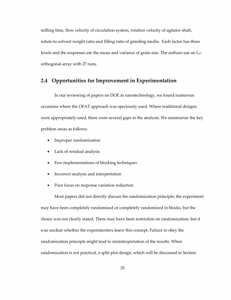
The multistage split-plot (MSSP) design is an extension of the split-plot design,
and can be thought of as having a single whole plot and a subsequent series of subplots
(Acharya and Nembhard, 2008). The format of the series of subplots can be split-plot
structure or split-block structure based on the nature of the experimentation. Vivacqua
and Bisgaard (2004, 2009), Acharya and Nembhard (2008), and Yuangyai et al. (2009)
suggest applying the split-plot, split-block, and combination of split-plot and split-block
structures to the multiple stage experiment. The MSSP design considerably decreases the
number of settings in experiments.
To reduce the number of settings and the number of runs in experimentation
while maintaining design efficiency, we posit that combining the MSSP and FFSP will be
an effective alternative. We refer to this design as the multistage fractional factorial split-
plot (MSFFSP) design.
1.4.2 Robust Parameter Design for Multistage Experimentation
Oftentimes, new products are successfully produced in laboratory settings but
when they are transitioned to full-scale manufacturing process the results are reversed
due to the fluctuations of uncontrollable factors such as process parameters, raw
materials, and customer uses. To solve these problems, Taguchi (1987) introduced the

15
concept of robust parameter design (RPD) to the quality engineering community.
RPD is a methodological technique to deal with two types of factors: controllable
and uncontrollable (noise) factors. The objective of RPD is to determine at which
controllable factors level to provide the output performance reaching the target desire
while the variability of the output is minimal when it is under noise factors.
For example, in the particle preparation stages of the lost mold rapid infiltration
process, there are five factors of interest: solids loading, gel, binder, milling time, and
milling chamber temperature. In laboratory settings, all five factors can be controlled;
however, when these stages are transferred to the manufacturing scales, the temperature
becomes difficult to control due to changes in the weather.
Little research focuses on RPD with restrictions on randomization. Recent
developments are discussed in Bingham and Sitter (2003) who study how to use the
split-plot design for RPD purposes. Therefore, it is necessary to develop a multistage
experimentation design with the RPD concept to facilitate situations where restriction on
randomization exists.
1.5 Research Objectives
The goal of this research is to develop an integrated framework for DOE and
RPD analysis to expedite the transition of micro- and nano-scale technologies into robust
products that can be produced with minimum variability and defects. In developing a
new manufacturing process for micro- and nano-scaled devices, due to its complexity,

16
there are ‚hard-to-change‛ product and process variables. Some of these hard-to-change
variables can have a compound effect on how parameters should be set across the stage
of the manufacturing process. Furthermore, the transfer from laboratory to
manufacturing settings often causes many discrepancies in terms of output performance
and process variability. While a rich history and body of literature on DOE and RPD
exists, there is a gap between the literature and the existing problem.
The objectives of this research project are to develop and analyze experimental
designs to:
1) incorporate the critical characteristics of multiple stage processing in micro- and
nano-scale manufacturing; and
2) integrate the concept of RPD in micro- and nano-scale new product
development.
We recognize the broad implications of developing a framework to understand
how to establish new products and processes at the nano-scale. In addition, there is the
potential of the work to be extended to other types of components beyond MIS
instrumentation.
1.6 Research Contributions
The research contributions are summarized as follows:
1. As only a multistage split-plot and multistage split-block model is currently
available, we extend the modeling and analysis of MSFFSP with the

17
combination of split-plot and split-block structure. This model is an
alternative for an experimenter who needs to reduce the number of settings
and number of runs, while maintaining design efficiency in experimentation.
However, the MSFFSP design disadvantages include difficulties to analyze the
data due to multiple errors terms and limited number of degree of freedom.
2. Optimal design catalogs for MSFFSP design are constructed based maximum
resolution and minimum aberration criteria. These catalogs help the
experimenter to obtain as much information as possible.
3. As an integration framework of MSFFSP design and RPD study is developed,
it will assist experimenters in avoiding the interaction between controllable
factors and noise factors. It will also allow us to identify sources of variability
in experimental data that reflect actual variability when the new process is
transferred to the manufacturing stage.
4. We illustrate the use of MSFFSP design and analysis as well as integration
with RPD by experimentation on the process to develop the FS instrument.
We believe the use of these models will be applicable to other areas.
1.7 Outline of the Dissertation
This research proposal is organized as follows. In Chapter 2, the literature review
related to DOE methods is discussed. Next, the MSFFSP design and analysis are
discussed in Chapter 3, followed by the optimal design for MSFFSP design in Chapter 4.

18
The robust parameter design with MSFFSP design and analysis are presented in Chapter
5. Finally, Chapter 6 provides a conclusion and direction for future research.

19
Chapter 2.
Literature Review
At the nano-scale, there are often very complex relationships among input design
parameters and process or product outputs. It would be prohibitively time consuming to
perform all of the combinatorially possible experiments in order to comprehend these
relationships. However, statistical design of experiments (DOE) is a technique that can
be used to efficiently explore the relationships and develop greater understanding.
Consequently, DOE is becoming increasingly central to the advancement of
nanotechnology and nanomanufacturing.
In this chapter, we begin with an introduction to DOE in Section 2.1. In Section
2.2, we discuss the one-factor-at-a-time (OFAT) approach which is often used among
scientists and engineers. In Section 2.3, we consider traditional methods implemented in
nanotechnology experimentation in practice. Opportunities for improvement are given
in Section 2.4. In Section 2.5, we propose modern DOE methods that are appropriate for
nanotechnology and nanomanufacturing. Section 2.6 provides a table of suggested DOE
methods that map to particular areas within nanotechnology as well as a table of all of
the articles in nanotechnology that we reviewed for this chapter that use statistical
experimentation. Section 2.7 gives some editorial remarks.
20
2.1 Introduction to Design of Experiments
DOE has been used in agriculture trials for over 70 years. Much of the early work
was conducted at the Rothamsted Experiment Station in England by R.A. Fisher
(Giesbrecht and Gumpertz, 2004, Ryan, 2007, Montgomery, 2009). The use of DOE then
spread to other areas such as the pharmaceutical industry, continuous and discrete
production processes, bio assay procedures, clinical trials, psychological experiments,
laboratory analysis, as well as business and economics studies (Neter et al., 1990,
Giesbrecht and Gumpertz, 2004).
Notwithstanding, the use of DOE is fairly uncommon in the field of
nanotechnology. One impediment is the lack of similar terminologies. For example,
‚parameter‛ refers to a controlled variable affecting the output of interest in
nanotechnology, whereas this term is referred to as a ‚factor‛ in a DOE context. In order
to establish a clear basis, we introduce some common DOE terminology as follows:
A Factor is a controllable variable of interest. The factor can be either
quantitative or qualitative. A quantitative factor can be measured on a numerical
scale. Some examples of a qualitative factors include the temperature of a
furnace, amount of a chemical, ratio of a material portion, weight of a substrate,
etc. A qualitative factor can be categorized into a group. Examples include type
of material, suppliers, operators, etc.
Factor levels are different values or types of factors in the range of interest.
A treatment or a treatment combination is one of the possible combinations

21
among all the factors level that apply to an experimental unit.
An Experimental unit is the smallest unit (it can be a physical unit or a
subject) to which one treatment combination applied independently.
A run or trial is an implementation of a treatment combination to an
experimental unit. Similar treatment combinations can be applied to several
different experimental units.
A Response is a qualitative or quantitative characteristic of an
experimental unit measured after we apply a treatment combination.
Understanding the response is regularly an objective of the experiment.
In order to obtain an appropriate design and analysis, Fisher (1966) identifies
three fundamental principles in performing the experiment: randomization, local control
(also called blocking), and replications. These can be explained as follows.
Randomization is a process that collects all sources of variation affecting the
treatment effects except those due to treatment itself. The randomization tends to
reduce the confounding of uncontrolled factors and controlled factors. It is very
important in experimental analysis because it is required to have a valid
estimation of random error3.
Local control or blocking is a technique that is used to segregate an uncontrolled
but known variation in an experiment not associated with the treatment effect.
3 This generally appears in analysis of variance (ANOVA) table which is a technique used to partition the total
variation into the variation of each of the source of variation listed in a response model.

22
The blocking should be designed to have maximum variation among blocks
(heterogeneous between blocks) but to have minimum variation with blocks
(homogeneous within blocks).
Replication refers to the replication of a treatment combination. It is needed for a
specific degree of precision for measuring treatment effects. It should be carefully
noted that replications are not multiple readings. Replication requirements are
stringent: to assure a proper replication, experimenters must reset every
condition in the experiment. If the treatment combinations are not reset, the
errors in the multiple readings are not independent. This, in turn, leads to the
violation of the randomization principle.
2.2 OFAT: The Predominant Method Used in Practice
The one factor at a time (OFAT) method is a basic approach that has been widely
used in science and engineering experimentation. The OFAT method is performed by
selecting a starting baseline by varying one factor level at a time while keeping other
factor levels constant. Then, the experimenter determines which level provides the best
result; that factor level is kept constant and the other factor levels are varied
sequentially. This method is methodological and may be suitable for some cases
depending upon the experimenter’s objectives. However, this method is not able to
estimate interaction effects among the factors. Furthermore, there is no guarantee that
the combination of the levels will provide optimal results (Daniel, 1973, Giesbrecht and

23
Gumpertz, 2004, Box, 2006, Ryan, 2007, Montgomery, 2009) .
Ryan (2007) provides a good example of an experiment where interaction among
factors cannot be estimated. Suppose that in an engineering department, two engineers
are asked to maximize process yield, where there are two factors of interest: temperature
(A) and pressure (B). Assume that the first engineer use the OFAT, whereas the second
engineer decides, to vary both factors simultaneously.
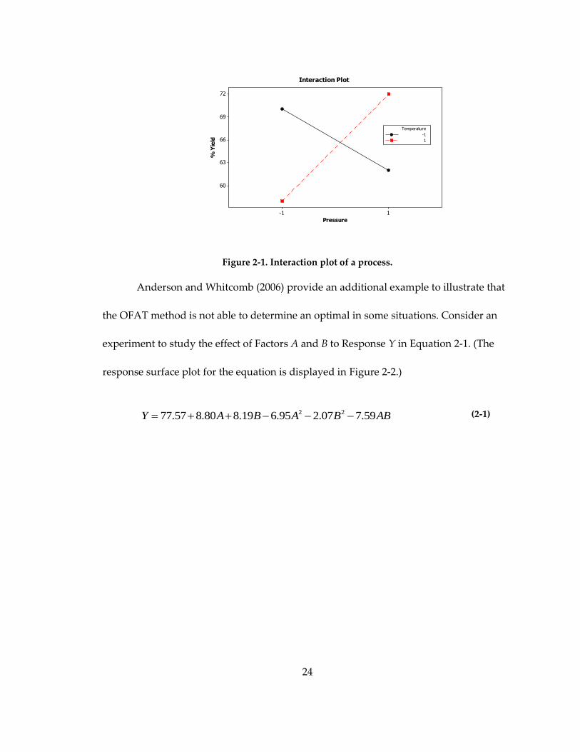
Assume the real process behaves as shown in Figure 2-1. If the first engineer
studies the process by initially keeping temperature at the low level and varying the
pressure from low to high, he would suggest that the best condition is to set the pressure
and temperature at the low level. However, if he starts the experiment by setting this
temperature at a high level and then varying the pressure, he would suggest the
opposite: to keep the pressure at a low level when the temperature is high. The results
could become rather confusing and possibly erroneous.
On the other hand, the second engineer does the experiment by considering all
treatment combinations. The results would lead him to conclude that it is best to use
high temperature and high pressure or low temperature and low pressure to increase
the yield due to interaction phenomenon of the temperature and the pressure.
24
Pressure
% Y
ield
1-1
72
69
66
63
60
Temperature
-1
1
Interaction Plot
Figure 2-1. Interaction plot of a process.
Anderson and Whitcomb (2006) provide an additional example to illustrate that
the OFAT method is not able to determine an optimal in some situations. Consider an
experiment to study the effect of Factors A and B to Response Y in Equation 2-1. (The
response surface plot for the equation is displayed in Figure 2-2.)
2 277.57 8.80 8.19 6.95 2.07 7.59Y A B A B AB (2-1)

25
Figure 2-2. OFAT experimentation.
If the experimenter varies Factor A from -2 to +2 and then plots a graph in Figure
2-2 (bottom left), it can be seen that the response Y is maximized when Factor A is set at
0.63. Following the OFAT method, the experimenter will keep Factor A at 0.63 as a
constant then vary Factor B. The result indicates that now the response increases from 80
to 82 by adjusting Factor B to 0.82 as shown in Figure 2-2 (bottom right). If we employ
OFAT, it would suggest keeping Factor A at 0.63 and Factor B at 0.82 in order to
maximize the response. However, in the real process Figure 2-2 (top), it can be clearly
seen that the Response Y can be increased up to 94.
From these two brief illustrations, it is easy to see why the OFAT approach is not
recommended for experimentation. Nevertheless, the OFAT method is widely used.
Anderson and Whitcomb (2007) suggested that a possible reason for this unfortunate

26
reality is because most basic coursework introduces and encourages the use of this
method. As demonstration, they provided an example that a physical science text for
ninth-graders in the US suggests using the OFAT for a motion experiment. Since DOE
coursework is not required across all science disciplines, OFAT often carries into
industrial, and even non statistical-academic settings.
We reviewed several articles that appeared in Nanotechnology and found that the
OFAT method has been used in many published papers: Unalan and Chhowalla (2005),
Pan et al. (2005), Buzea et al. (2005), Zhang et al. (2005), Xue et al. (2005), Dimaki et al.
(2005), Chen et al. (2006), Kim et al. (2006), Chen et al. (2006), Huang et al. (2006), Li et al.
(2006), Lee and Liu (2007), Mattila et al. (2007), Kim et al. (2007), Plank et al. (2008), and
Schneider (2009).
In the next sections, we will discuss several DOE methodologies that can be used
by experimenters in the nanotechnology field to gain a better understanding of a
process.
2.3 Traditional Methods used in Research and Development
In reviewing the literature that properly uses DOE in nanotechnology and
nanomanufacturing, we found that four types of traditional designs are employed:
completely randomized design (CRD); two-level factorial or fractional factorial design;
response surface methodology (RSM); and Taguchi’s method. The relevant articles are
summarized in Table 2-1. Even though these methods are relevantly recently applied in
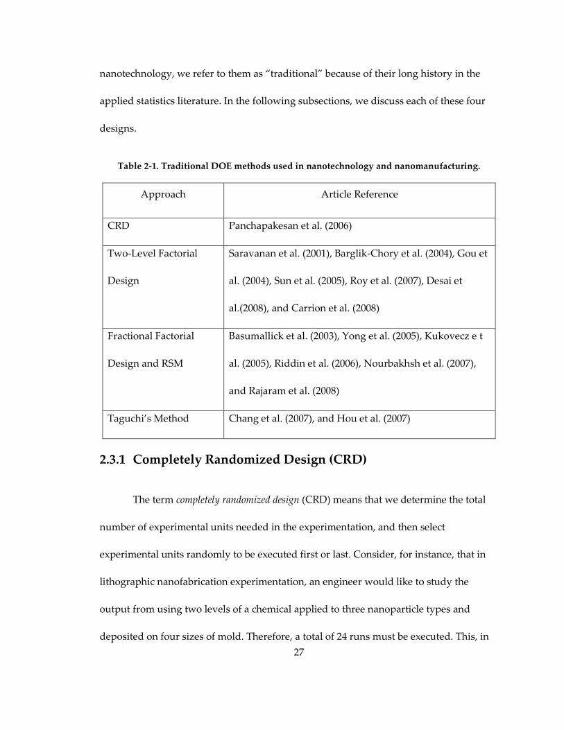
27
nanotechnology, we refer to them as ‚traditional‛ because of their long history in the
applied statistics literature. In the following subsections, we discuss each of these four
designs.
Table 2-1. Traditional DOE methods used in nanotechnology and nanomanufacturing.
Approach Article Reference
CRD Panchapakesan et al. (2006)
Two-Level Factorial
Design
Saravanan et al. (2001), Barglik-Chory et al. (2004), Gou et
al. (2004), Sun et al. (2005), Roy et al. (2007), Desai et
al.(2008), and Carrion et al. (2008)
Fractional Factorial
Design and RSM
Basumallick et al. (2003), Yong et al. (2005), Kukovecz e t
al. (2005), Riddin et al. (2006), Nourbakhsh et al. (2007),
and Rajaram et al. (2008)
Taguchi’s Method Chang et al. (2007), and Hou et al. (2007)
2.3.1 Completely Randomized Design (CRD)
The term completely randomized design (CRD) means that we determine the total
number of experimental units needed in the experimentation, and then select
experimental units randomly to be executed first or last. Consider, for instance, that in
lithographic nanofabrication experimentation, an engineer would like to study the
output from using two levels of a chemical applied to three nanoparticle types and
deposited on four sizes of mold. Therefore, a total of 24 runs must be executed. This, in

28
turn, implies that the experimenter would have to make 24 slurry preparations and
apply each to 24 molds. If experimenters make only six slurry preparations and then
divide the slurry to four portions and then deposit on the different molds, this
procedure is not a CRD. (To overcome this situation in practice, we suggest the use of a
split-plot design and its variants.)
The term factorial design which can be also called combination design or crossed
design means that all combinations of factor levels are executed. It is an efficient
approach when two or more factors are considered because factor interactions can be
estimated (Montgomery, 2009). However, the factorial design can be quite burdensome
because it requires the experimenter perform all possible combinations of all factor
levels. For example, consider a process that has two factors and each factor has four and
five levels, respectively. In this case, a total of 20 combinations must be randomized and
tested.
Example: Factorial design in a tin-oxide nanostructure synthesis process
Panchapakesan et al. (2006) studied the effects of seven gas types, three levels of
concentrations, six different types of seeded sensor (SnO2) and six grain size diameters
for the sensitivity of tin-oxide nanostructures on large area arrays of micro hotplates. In
this case, the authors used the full factorial design. There were 7×3×6×6 = 756 runs which
they claimed to be randomized using sophisticated software program. They presented
the results of the experiment using a graphical method.
An analysis of variance (ANOVA) would typically be conducted because we can

29
estimate the interaction of all four factors and also use the two-level factorial designs
with center points to reduce the number of run experimental runs.
2.3.2 Two-level Factorial Design
Two-level Full Factorial Design
Like the factorial design, the two-level factorial design requires all possible
combinations to be executed. However, instead of using several levels of each factor,
only two levels are selected. This design is helpful when used in the beginning of an
experimental effort in order to select only the potential significant factors, especially if
the experimenter has limited knowledge of the experiment.
Example: Two-level full factorial design in a single-wall nanotubes synthesis
process
Gou et al. (2004) provide a good example of using a two-level factorial design to
study the effect concentration of suspension, sonication time, and vacuum pressure to
the average and standard deviation of rope and pore size of single wall nanotubes
(SWNTs). Then they estimate the relationships between the response and factor by using
a regression method without the second-order effect. The authors could not optimize the
process, so further experimentation is required. Response surface methodology (RSM)
would be helpful to optimize the processes.

30
Two-level Fractional Factorial Design
If there are k factors of interest and the two-level factorial design is used, the
number of treatment combinations increases rapidly as k increases: the total number of
treatment combinations is 2k. However, under the assumption that the higher order
interactions have a smaller effect on the output compared to the main effects or the
second order effects, we can improve the cost and time of experimentation by reducing
the number of experiments by a half or even a quarter or an eighth of the original
design. With fewer experiments, there will be a loss of some information. A two-level
fractional factorial design is generally expressed in the form of 2k-p, where p is the
fraction of the full 2k factorial (that is, 1/2p).
Once a few key factors are determined, the experimenter may want to improve
the process by trying to optimize the process output. In this case, response surface
methodology (RSM) will be employed. This approach allows the experimenters to
estimate the second-order effect of factors that cannot be estimated from the two-level
factorial designs.
Example: Two-Level Fractional Factorial Design in a Single-Wall Carbon
Nanotubes Synthesis Process
Kukovecz et al. (2005) reported the use of a 27-4 design to study the effect of seven
factors on the carbon percentage and the quality descriptor number (QDN). The factors
are reaction temperature, reaction time, preheating time, catalyst mass, C2H2 volumetric
flow rate Ar volumetric flow rate and Fe:MgO molar ratio. The design is a resolution III
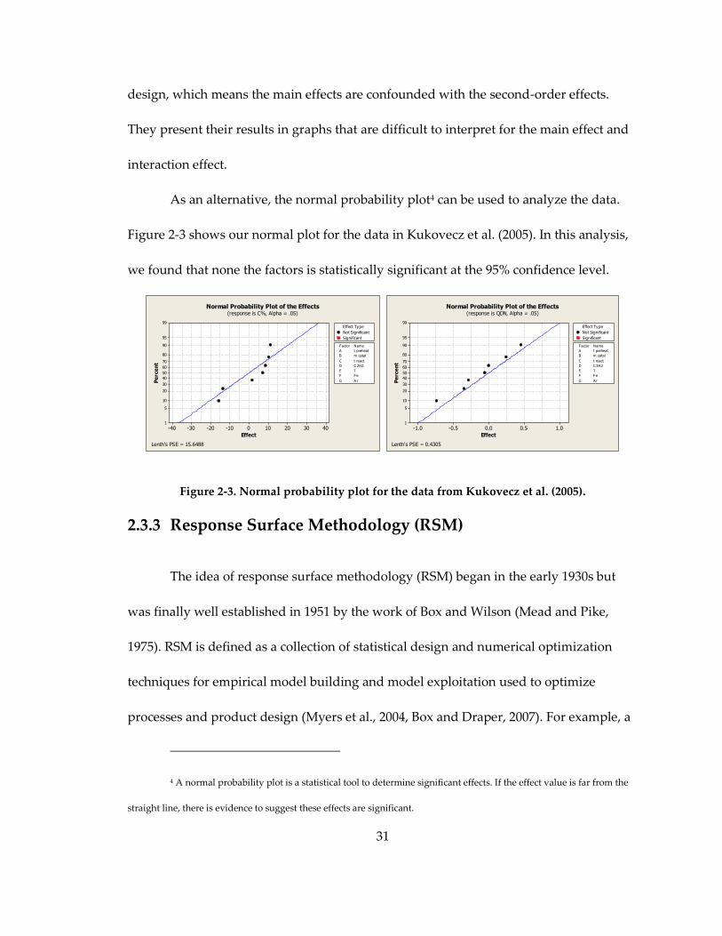
31
design, which means the main effects are confounded with the second-order effects.
They present their results in graphs that are difficult to interpret for the main effect and
interaction effect.
As an alternative, the normal probability plot4 can be used to analyze the data.
Figure 2-3 shows our normal plot for the data in Kukovecz et al. (2005). In this analysis,
we found that none the factors is statistically significant at the 95% confidence level.
Effect
Pe
rce
nt
403020100-10-20-30-40
99
95
90
80
70
60
50
40
30
20
10
5
1
Factor
C 2H2
E T
F Fe
G A r
Name
A t preheat
B m catal
C t react
D
Effect Type
Not Significant
Significant
Normal Probability Plot of the Effects(response is C%, Alpha = .05)
Lenth's PSE = 15.6488 Effect
Pe
rce
nt
1.00.50.0-0.5-1.0
99
95
90
80
70
60
50
40
30
20
10
5
1
Factor
C 2H2
E T
F Fe
G A r
Name
A t preheat
B m catal
C t react
D
Effect Type
Not Significant
Significant
Normal Probability Plot of the Effects(response is QDN, Alpha = .05)
Lenth's PSE = 0.4305
Figure 2-3. Normal probability plot for the data from Kukovecz et al. (2005).
2.3.3 Response Surface Methodology (RSM)
The idea of response surface methodology (RSM) began in the early 1930s but
was finally well established in 1951 by the work of Box and Wilson (Mead and Pike,
1975). RSM is defined as a collection of statistical design and numerical optimization
techniques for empirical model building and model exploitation used to optimize
processes and product design (Myers et al., 2004, Box and Draper, 2007). For example, a
4 A normal probability plot is a statistical tool to determine significant effects. If the effect value is far from the
straight line, there is evidence to suggest these effects are significant.
32
chemical engineer wishes to find the levels of temperature (X1) and pressure (X2) that
maximize the yield (Y) of a process. The process yield is a function of the levels of
temperature and pressure
1 2( , )y f x x
where ε is the error observed in the response Y. If the expected response is
1 2( ) ( , )E y f x x
then the surface is represented by
1 2( , )f x x
RSM is considered a sequential approach and consists of three steps: screening,
region seeking, and product/process characterization. Screening investigates which
factors of interest are significant. Note that the method is used in this stage can be a two-
level (fractional) factorial design. The surface can be estimated by the following first-
order model:
0 1 1 2 2 k ky x x x
The next step is to know whether the current response situation is in the optimal
region. If not, we have to employ region seeking to find a path to an optimal region.
Once the region is determined, the process phenomena can be estimated by a second-
order model:
2
0
1 1
k k
i i ii i ij i j
i i i j
y x x x x
The response surface is shown graphically as demonstrated in Figure 2-4. To
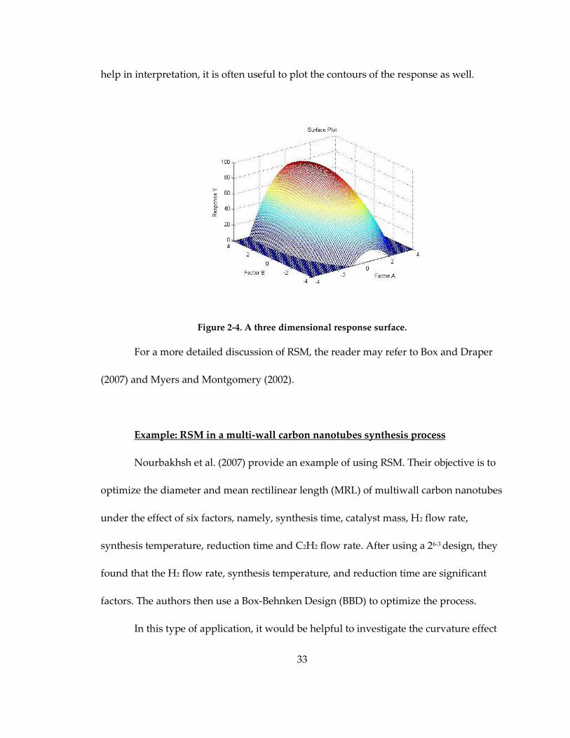
33
help in interpretation, it is often useful to plot the contours of the response as well.
Figure 2-4. A three dimensional response surface.
For a more detailed discussion of RSM, the reader may refer to Box and Draper
(2007) and Myers and Montgomery (2002).
Example: RSM in a multi-wall carbon nanotubes synthesis process
Nourbakhsh et al. (2007) provide an example of using RSM. Their objective is to
optimize the diameter and mean rectilinear length (MRL) of multiwall carbon nanotubes
under the effect of six factors, namely, synthesis time, catalyst mass, H2 flow rate,
synthesis temperature, reduction time and C2H2 flow rate. After using a 26-3 design, they
found that the H2 flow rate, synthesis temperature, and reduction time are significant
factors. The authors then use a Box-Behnken Design (BBD) to optimize the process.
In this type of application, it would be helpful to investigate the curvature effect

34
by adding center points and checking whether or not the optimal condition is in the
range of interest. If not, path searching should be done before completely employing the
BBD. The response surface graph demonstrates that the current solution is not yet
within the optimal region.
2.3.4 Taguchi’s Method
Genichi Taguchi’s methods have been widely known in industry for decades.
The central idea of his methods are the quality loss function and robust parameter
design (Taguchi et al., 1999, Taguchi et al., 2005). The quality loss function is used to
estimate costs when the product or process characteristics are shifted from the target
value. This is represented by the following equation:
2( ) ( )L y k y T
where L(y)is a cost incurred when the characteristic y is shifted from the target T and k is
constant depending on the process. This concept is known as parameter design, which is
a selection of a parameter level in order to make the process robust against
environmental changes with minimum variation.
There have been some criticisms of Taguchi’s approach in the applied statistics
literature. For example, it sometimes fails sometimes to consider the interaction effect of
factors much like fractional factorial design (Montgomery, 1996).
Example: Taguchi’s method in a nanoparticle wet milling process
Hou et al. (2007) applied the Taguchi method to study the effects of five factors:
35
milling time, flow velocity of circulation system, rotation velocity of agitator shaft,
solute-to solvent weight ratio and filling ratio of grinding media. Each factor has three
levels and the responses are the mean and variance of grain size. The authors use an L27
orthogonal array with 27 runs.
2.4 Opportunities for Improvement in Experimentation
In our reviewing of papers on DOE in nanotechnology, we found numerous
occasions where the OFAT approach was speciously used. Where traditional designs
were appropriately used, there were several gaps in the analysis. We summarize the key
problem areas as follows:
Improper randomization
Lack of residual analysis
Few implementations of blocking techniques
Incorrect analysis and interpretation
Poor focus on response variation reduction
Most papers did not directly discuss the randomization principle; the experiment
may have been completely randomized or completely randomized in blocks, but the
choice was not clearly stated. There may have been restriction on randomization, but it
was unclear whether the experimenters knew this concept. Failure to obey the
randomization principle might lead to misinterpretation of the results. When
randomization is not practical, a split-plot design, which will be discussed in Section

36
2.5.1 and 2.5.2, can often be used.
A few papers did not mention whether the output was tested for normality and
independence. This issue here is that the variance will be underestimated if a positive
correlation among responses exists. This could lead the experimenters to conclude that
certain factors are significant when, in actuality, they are not. Repeated measures, which
will be discussed in Section 2.5.3, can be used to address this situation.
The blocking technique was rarely used in the literature. This technique is
beneficial for segregating the uncontrolled factors out of the model. It was unclear
whether readings in some experiments were papers are replications or mere multiple
readings.
RSM is quite popular in nanotechnology literature. However, in some cases, the
results have been interpreted incorrectly. For example, if a two-level factorial design is
used with center points, this only informs the experimenters as to whether there are
second order effects in the experimental region. It does not suggest which effect is
contributing the second order interaction. We also found that many papers fail to seek a
path to reach the optimal experiment condition, which is one of the main reasons for
employing RSM (Kukovecz et al., 2005, Yong and Hahn, 2005, Nourbakhsh et al., 2007).
Some papers fall short in the proper use of parameter estimation. It is not always
appropriate to keep all the parameter estimates in the model because some terms might
not be significant and should be ignored. On the other hand, some insignificant terms
may be maintained in order to adhere to the hierarchical principle. The point is to

37
carefully consider both sides of the issue.
Much of this work focuses on mean response and ignores the response
variability. In order to improve processes, we would like to have processes with both
desirable results and a minimum variation. This topic can be addressed using the quality
loss function concept suggested by Taguchi.
2.5 Modern DOE Methods Appropriate for Nanotechnology and
Nanomanufacturing
In practice, there are many restrictions on experimentation. These include the
randomization restriction on the treatment combination, the dependence of the factor
level, the restriction of treatment combination space, and constraints in physical
experiments. Therefore, there is a need for other kinds of design and analysis of
experiments that overcome those restrictions. We believe that the following designs can
be effectively used in the area of nanotechnology and nanomanufacturing:
Split-Plot Design (and its Variants)
Multistage Split-Plot Design
Repeated Measures
Super Saturated Design
Mixture Design
Computer Deterministic Experiments
Computer Aided Design (Alphabetical Optimal Design)

38
2.5.1 Split-Plot Design and its Variants
The designs that we have previously discussed are based on the complete
randomization principle. However, in many situations, it is impossible to randomize all
treatment combinations. In such cases, the split-plot design may be used. The name
‚split plot‛ comes from the agricultural experiment which the whole plots are
considered for large plot of land and the sub plots are used to represent small plot of
land within the large area.
The standard split-plot design is a design which has a two-factor factorial
arrangement. For example, Factor A with a levels, is designed as a randomized complete
design; the levels of Factor A treatments is called a whole plot experimental unit. The
each experimental unit is divided into b split-plot experimental units of Factor B.
The strip block5 design is another type of design which is bit different from the
split-plot design. This design has two factors, Factor A with a level and Factor B with b
level. The levels of Factor A are randomly assigned to the a whole plot experimental
unit. Then the B experimental units are formed perpendicular to the A experimental
unit, and the b levels of factor B are randomly allocated to the second set of b whole plot
units in each of the complete blocks.
Box and Jones (2000-01) discuss the CRD, split-plot design, and split block design
5 The strip block also known as split block design, strip plot design, two-way whole plot design and criss-cross
design (Federer 2007).

39
using a cake mixing experiment which consists of two processes: mixing and baking.
There are five factors with two levels each; three factors in the mixing process and two
factors in the baking process. If the CRD is used, 32 preparations for mixing and baking
are required.
On the other hand, the split-plot design requires fewer experimental resources
based on three cases. First, if the mixing factors are whole plot factors, eight cake-mixing
preparations are required. However; if the baking factors are whole plot factors, four
settings of a baking oven are prepared. Note that for the subplot factor setting in both
cases requires 32 preparations. In the split block arrangement, only eight mixes and four
bakes are required. Table 2-2 shows four possible arrangements for the different designs.
Table 2-2. Four possible arrangements for the cake mix experiment (Box and Jones, 2000-01).
Type of Design
Number of settings in
Mixes Bakes
Fully Randomized 32 32
Split-plot: Bakes are the subplot 8 32
Split-plot: Recipes are the subplot 32 4
Split block 8 4
This split-plot structure is a foundation of the multistage process design of
experiment. Further studies are provided by Kowalski and Potcner (2003), and Federer
and King (2007).

40
Example: Split-Plot Design and Split-Block Design in a Gel-Casting
Lithography Process
Yuangyai et al. (2009) discuss different arrangements of the split-plot and split
block design based on the process of making a ceramics parts using gel casting and
lithography method developed by Antolino et al. (2009a, 2009b). The process is
composed of six sub-processes: particle preparation, mold fabrication, monomer
addition, colloid deposition, sintering, and final dressing. We will use this process to
demonstrate the different arrangements of CRD, split-plot design, and split block
design.
Let us consider only two sub-processes – monomer addition and sintering – and
assume that there are two factors of interest: amount of ethylene glycol (d) and amount
of monomer (e), with two levels in the preparation process and two furnace conditions
(x) in the sintering process. If a CRD is used, eight samples are prepared at different
times, then each sample must be placed into a furnace at different times (see Figure
2-5a).
If the split-plot design is used, there are only four sample preparations required
and each sample is split into two sub-samples, then each subsample is placed into the
furnace at a different time. Therefore, there are four sample preparations and eight
sintering settings (see Figure 2-5b).
Whereas, in the split block design, only four samples are prepared and then each
is split into two sub-samples (similar to those in split-plot design). However, these sub-
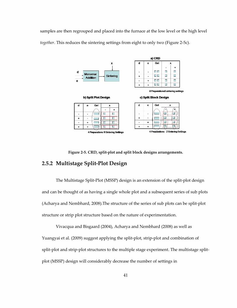
41
samples are then regrouped and placed into the furnace at the low level or the high level
together. This reduces the sintering settings from eight to only two (Figure 2-5c).
Figure 2-5. CRD, split-plot and split block designs arrangements.
2.5.2 Multistage Split-Plot Design
The Multistage Split-Plot (MSSP) design is an extension of the split-plot design
and can be thought of as having a single whole plot and a subsequent series of sub plots
(Acharya and Nembhard, 2008).The structure of the series of sub plots can be split-plot
structure or strip plot structure based on the nature of experimentation.
Vivacqua and Bisgaard (2004), Acharya and Nembhard (2008) as well as
Yuangyai et al. (2009) suggest applying the split-plot, strip-plot and combination of
split-plot and strip-plot structures to the multiple stage experiment. The multistage split-
plot (MSSP) design will considerably decrease the number of settings in

42
experimentations.
Example: MSSP Design in a Gel-Casting Lithography Process
Acharya and Nembhard (2008) used a multistage split-plot design in scaling up a
three-step surface initiated polymerization process-preparation of self-assembled
monolayer (SAM), anchoring catalyst on the SAM, and synthesis of polymer brush.
However, past literature indicates that the operative levels of the stage-one factors –
amount of gold evaporated, thickness of silicon wafer, amount of Cr, temperature and
time – are pre-determined. Therefore these factors are ignored in the experimentation.
Accordingly, the authors considered only the last two stages. There are four factors in
stage one: amount of catalyst, type of rinsing solvent, drying time, and reaction time.
There are three factors in stage two: reaction temperature, type of Ar flow, and reaction
time. The authors propose catalogs of fractional factorial split-plot design for three and
four stages according to optimal criteria: robustness and maximum number of mixed
three-way interaction.
2.5.3 Repeated Measures
The problem of designing a statistical experiment with repeated measures has
been extensively studied in the DOE literature. Repeated measures implies that
experimental units or subject will be used more than once (i.e., at two or more periods of
time) (Giesbrecht and Gumpertz, 2004). Consequently, any potential model for the
response variable in terms of the factors considered in the experiment will need to

43
contain parameters for unit or subject effects, period or time effects, and possible
carryover effects. Many repeated measures studies involve observations over time (or
space) and the evolution of response is often of special importance (Lindsey, 1999).
Because the same unit is producing several successive responses, those that are closer
together will tend to be more closely related; in other words, a previous result is playing
a role on the ensemble of the response variable realization. Therefore, in such cases,
these relationships must also be included in the model.
Example: Repeated Measures in a Nanopartical Wet Milling Process
Kumar et al. (2005) presented an experimental design to explore the significant
factors to efficiently mill alumina by a chemically aided attrition milling (CAAM)
process in nanophase alumina powder. Three factors – powder addition rate, media size
and agitator shaft speed – were studied. Each factor was tested at two levels with three
center points. These milling responses were recorded as average agglomeration number
(ANN) for one, two, three, or four hours of milling. The authors analyzed this
experiment by treating each response at different hour independently. However, these
data behaved dependently as the ANN at previous hour affects to the following hour.
The repeated measures analysis is more appropriate for this application.
2.5.4 Saturated and Supersaturated Design
In many nanotechnology and nanomanufacturing processes, the execution of
many runs is impractical due to limited resources. The idea behind the saturated and

44
super saturated designs is similar to fractional factorial design where the goal is not to
estimate all possible effects simultaneously but rather to screen several factors. Unlike
fractional factorial designs, the total number of runs in the super saturated design is less
than or equal to the number of factors. When the number of run is equal to the number
of factors, it is called a saturated design. When the number of runs is less than the
number of factors, it is called supersaturated design (Lin, 2003).
In order to obtain unbiased estimator of effects, the number of runs must be
equal to the number of factor effects to be estimated plus one. However, in a situation,
that the insignificant factors are not of interest, estimating all main effects may not be
useful if it is only the detection of a few important factors that is important. If the
number of active factors is small compared to the number of runs, the careful use of
biased estimates will still make it possible to identify significant factors.
Example: Supersaturated Design in Nanorod Fabrication
Acharya and Lin (2008) presented the use of supersaturated designs to study the
growth of ZnO nanorods with consistent measurement of surface roughness in the
process of ZnO fabrication process involving nine factors with two levels each:
substrate, carrier gas, process temperature, carrier gas flow rate, synthesis time, catalyst,
distance between powder and substrate, optical density and time for deposition. There
were only six runs required to study those nine factors.

45
2.5.5 Mixture Design
The mixture design is a class of experimentation that is different from the
previous designs we have discussed wherein the assumption is that all factor levels are
independent. In the case of the mixture design, there is an assumed relationship among
factors. Suppose that in a chemical mixing experiment of two chemicals, the
experimenter would like to test how the quantity of each chemical affects the properties
of mixed chemical. In this case we use the previous design. However, if the
experimenter would like to study the effect of chemical ratio of two substances such as
1:1 or 2:3, a mixture design is used under a constraint that summation of the ratio must
be equal to one (Nembhard et al., 2006).
The main distinction between mixture experiments and independent variable
experiments is that with the former, the input variables or components are non-negative
proportionate amounts of the mixture. Also, if expressed as a fraction of the mixture,
they must sum to one. If for some reason, the sum of the component proportions is less
than one, the variable proportions can be rewritten as scaled fractions so that the scaled
fractions sum to one.
When the mixture components are subject to the constraint that they must sum to
one, there are standard mixture designs for fitting standard models, such as Simplex-
Lattice designs and Simplex-Centroid designs. When mixture components are subject to
additional constraints, such as a maximum and/or minimum value for each component,
designs other than the standard mixture designs, such as constrained mixture designs or

46
Extreme-Vertices design, are appropriate.
2.5.6 Computer Deterministic Experiments
Some investigations in nanotechnology research use computer simulation to
explain physical phenomena. Much of this simulation requires running complex and
computationally expensive analysis and codes. Despite continuing increases in
computer processor speed and capabilities, the time and computational costs of running
complex algorithms are high.
A way to overcome this problem is to generate an approximation of complex
analysis code that describes the process accurately, but at a much lower cost.
Metamodels offer an approximation as in that they provide a ‚model of the model‛.
Clarke et al. (2005) suggested metamodeling techniques, namely Response Surface
Methodology (RSM), Radial Basis Function (RBF), Kriging Model, and Multivariate
Adaptive Regression Splines (MARS) as potentially useful approaches. Computer
deterministic experiments have been addressed by Charles et al. (1996), Simpson et al.
(1998), Cappelleri et al. (2002), and Aguirre et al. (2008a).
2.5.7 Computer Generated Design: Alphabetical Optimal Design
In some experiment situations, it is not possible to experiment over all factor
regions and the experimenter cannot use any standard design. In these cases, computer-
generated (optimal) designs are alternatives to be considered. These designs are

47
optimized based on some user selected criterion and a prescribed experimental process
(a model is known). The concept of this approach is to generate all possible design sets
and then use search methods to determine which set of designs provide the best result.
In general, there are four types of optimal designs. Their names are based on the
alphabet so these designs are called alphabetical optimal design.
The D-Optimal design seeks to maximize the determinant of the information
matrix of the design. This criterion results in minimizing the generalized
variance of the parameter estimates based on a pre-specified model.
The A-Optimal design seeks to minimize the trace of the inverse of the
information matrix. This criterion results in minimizing the average variance of
the parameter estimates based on a pre-specified model.
The G-Optimal design seeks to minimize the maximum prediction variance over
a specified model.
The V-Optimal design seeks to minimize the average prediction variance over a
specified set of design points.
Since the optimality criterion of most computer-aided designs is based on some
function of the information matrix that the experimenter must specify a model for the
design and the final number of design points desired before the optimal design can be
generated. The design generated by the computer algorithm is optimal only for that
model. Alphabetical Optimal Designs are used by Charles et al. (1996), Hooker et al.
(2003) and Chuang et al. (2004).

48
2.6 Summary of Nanotechnology Articles that use Statistical
Experimentation
It is quite evident from the above discourse that modern DOE techniques have a
potential to be used in nanotechnology and nanomanufacturing. Table 2-3 gives a brief
summary of the DOE methods we have considered in this chapter along with the
nanotechnology areas in which they may be potentially useful.
Table 2-3. DOE method and nanotechnology mapping.
Method Summary
Potential Nanotechnology
Applications
Split-plot Design and
Multi-Stage Split-plot
Design
This design is suitable for the
randomization restrictions that
frequently occur in experimentation.
The key concept of this design is that
there is more than one error structure
that experimenter must analyze. The
MSSSP design can be extended to
more than two processes.
Lithography
Process, Coating Process,
Plasma Arcing Process,
Nanoelement Assembly
Process, Laser-based
Synthesis Process, etc.
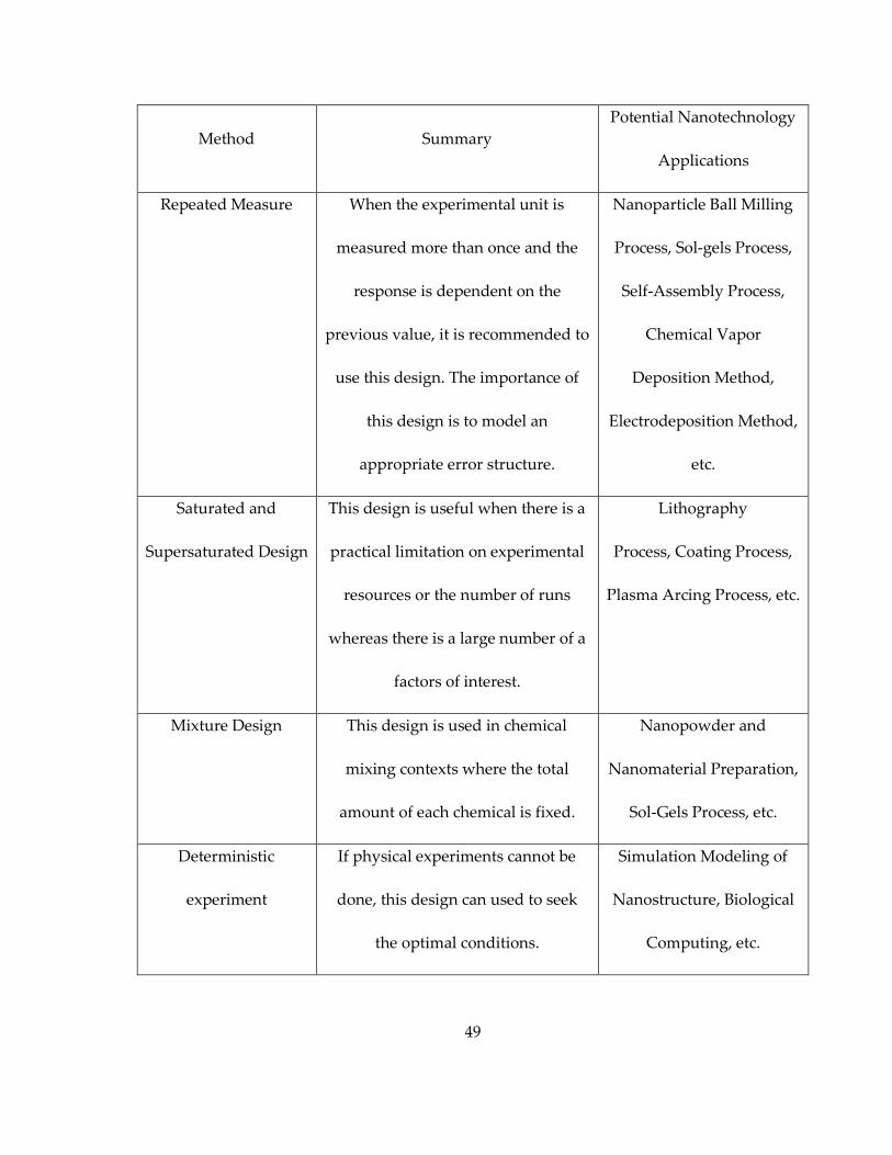
49
Method Summary
Potential Nanotechnology
Applications
Repeated Measure When the experimental unit is
measured more than once and the
response is dependent on the
previous value, it is recommended to
use this design. The importance of
this design is to model an
appropriate error structure.
Nanoparticle Ball Milling
Process, Sol-gels Process,
Self-Assembly Process,
Chemical Vapor
Deposition Method,
Electrodeposition Method,
etc.
Saturated and
Supersaturated Design
This design is useful when there is a
practical limitation on experimental
resources or the number of runs
whereas there is a large number of a
factors of interest.
Lithography
Process, Coating Process,
Plasma Arcing Process, etc.
Mixture Design This design is used in chemical
mixing contexts where the total
amount of each chemical is fixed.
Nanopowder and
Nanomaterial Preparation,
Sol-Gels Process, etc.
Deterministic
experiment
If physical experiments cannot be
done, this design can used to seek
the optimal conditions.
Simulation Modeling of
Nanostructure, Biological
Computing, etc.

50
Method Summary
Potential Nanotechnology
Applications
Alphabetic optimal
design
This design can be used in a situation
wherein the experimenters cannot
perform all possible experimental
regions of the factors.
All the above
Table 2-4 summarizes the 42 articles we examined for this chapter. They are
listed in order of the experimental method used and then by year of publication.

51
Table 2-4. Summary of Articles in Nanotechnology
Item Authors Year Technique Title
1 Unalan and Chhowalla 2005 OFAT
Investigation of Single-walled Carbon Nanotube
Growth Parameters Using Alcohol Catalytic Chemical
Vapour Deposition
2 Pan et al. 2005 OFAT
Surface Crystallization Effects on the Optical and
Electric Properties of CdS nanorods
3 Buzea et al. 2005 OFAT
Control of Power Law Scaling in the Growth of Silicon
Nanocolumn Pseudo-Regular Arrays Deposited by
Glancing Angle Deposition
4 Zhang et al. 2005 OFAT
Microstructure and Magnetic Properties of Ordered
La0.62Pb0.38MnO3 Nanowire Arrays

52
Item Authors Year Technique Title
5 Xue et al. 2005 OFAT
In Situ Fabrication and Characterization of Tungsten
nanodots on SiO2/Si via Field Induced Nanocontact
with a Scanning Tunnelling Microscope
6 Dimaki et al. 2005 OFAT
Frequency Dependence of the Structure and Electrical
Behaviour of Carbon Nanotube Networks Assembled
by Dielectrophoresis
7 Chen et al. 2006 OFAT
The Influence of Oxygen Content in the Sputtering Gas
on the Self-synthesis of Tungsten Oxide Nanowires on
Sputter-deposited Tungsten Films
8 Kim et al. 2006 OFAT
The Effect of Metal Cluster Coatings on Carbon
Nanotubes
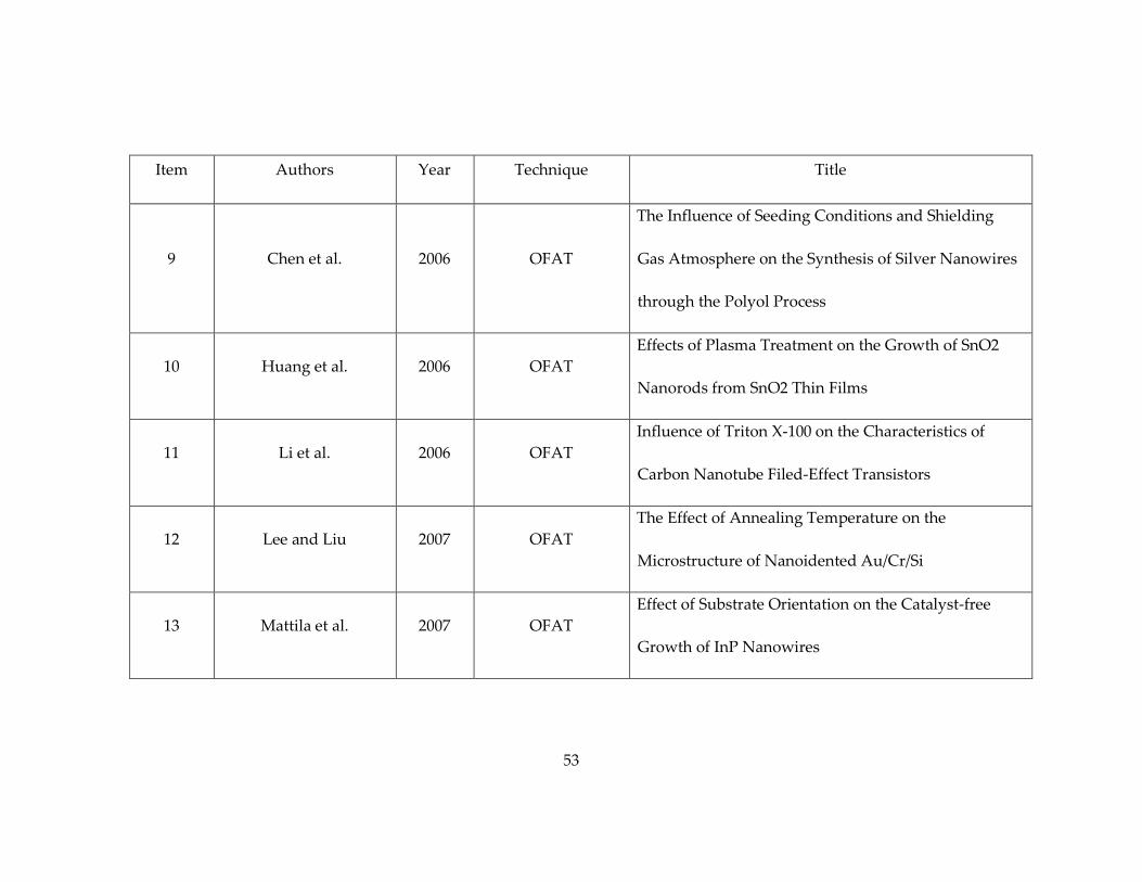
53
Item Authors Year Technique Title
9 Chen et al. 2006 OFAT
The Influence of Seeding Conditions and Shielding
Gas Atmosphere on the Synthesis of Silver Nanowires
through the Polyol Process
10 Huang et al. 2006 OFAT
Effects of Plasma Treatment on the Growth of SnO2
Nanorods from SnO2 Thin Films
11 Li et al. 2006 OFAT
Influence of Triton X-100 on the Characteristics of
Carbon Nanotube Filed-Effect Transistors
12 Lee and Liu 2007 OFAT
The Effect of Annealing Temperature on the
Microstructure of Nanoidented Au/Cr/Si
13 Mattila et al. 2007 OFAT
Effect of Substrate Orientation on the Catalyst-free
Growth of InP Nanowires
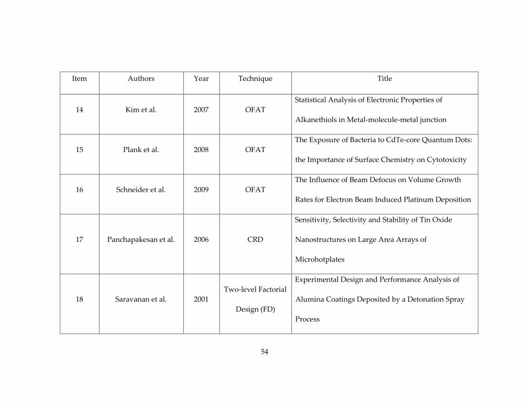
54
Item Authors Year Technique Title
14 Kim et al. 2007 OFAT
Statistical Analysis of Electronic Properties of
Alkanethiols in Metal-molecule-metal junction
15 Plank et al. 2008 OFAT
The Exposure of Bacteria to CdTe-core Quantum Dots:
the Importance of Surface Chemistry on Cytotoxicity
16 Schneider et al. 2009 OFAT
The Influence of Beam Defocus on Volume Growth
Rates for Electron Beam Induced Platinum Deposition
17 Panchapakesan et al. 2006 CRD
Sensitivity, Selectivity and Stability of Tin Oxide
Nanostructures on Large Area Arrays of
Microhotplates
18 Saravanan et al. 2001
Two-level Factorial
Design (FD)
Experimental Design and Performance Analysis of
Alumina Coatings Deposited by a Detonation Spray
Process
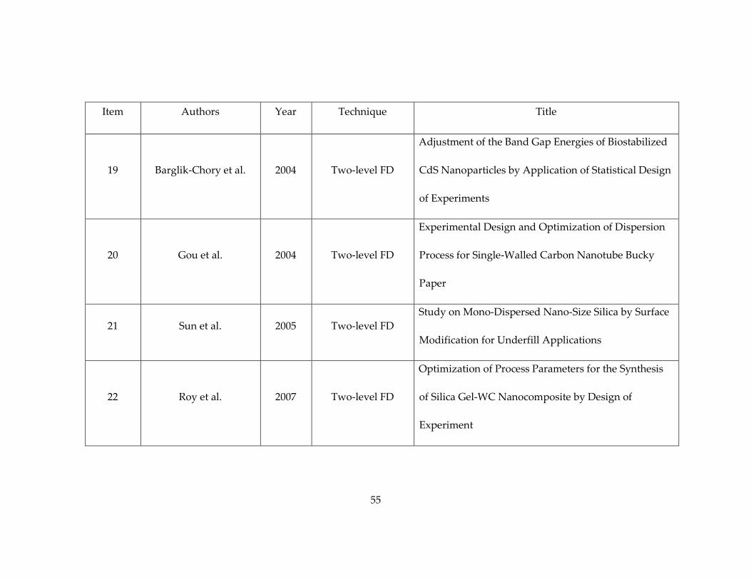
55
Item Authors Year Technique Title
19 Barglik-Chory et al. 2004 Two-level FD
Adjustment of the Band Gap Energies of Biostabilized
CdS Nanoparticles by Application of Statistical Design
of Experiments
20 Gou et al. 2004 Two-level FD
Experimental Design and Optimization of Dispersion
Process for Single-Walled Carbon Nanotube Bucky
Paper
21 Sun et al. 2005 Two-level FD
Study on Mono-Dispersed Nano-Size Silica by Surface
Modification for Underfill Applications
22 Roy et al. 2007 Two-level FD
Optimization of Process Parameters for the Synthesis
of Silica Gel-WC Nanocomposite by Design of
Experiment
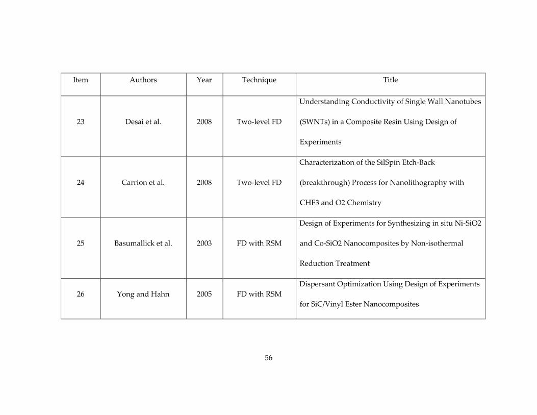
56
Item Authors Year Technique Title
23 Desai et al. 2008 Two-level FD
Understanding Conductivity of Single Wall Nanotubes
(SWNTs) in a Composite Resin Using Design of
Experiments
24 Carrion et al. 2008 Two-level FD
Characterization of the SilSpin Etch-Back
(breakthrough) Process for Nanolithography with
CHF3 and O2 Chemistry
25 Basumallick et al. 2003 FD with RSM
Design of Experiments for Synthesizing in situ Ni-SiO2
and Co-SiO2 Nanocomposites by Non-isothermal
Reduction Treatment
26 Yong and Hahn 2005 FD with RSM
Dispersant Optimization Using Design of Experiments
for SiC/Vinyl Ester Nanocomposites
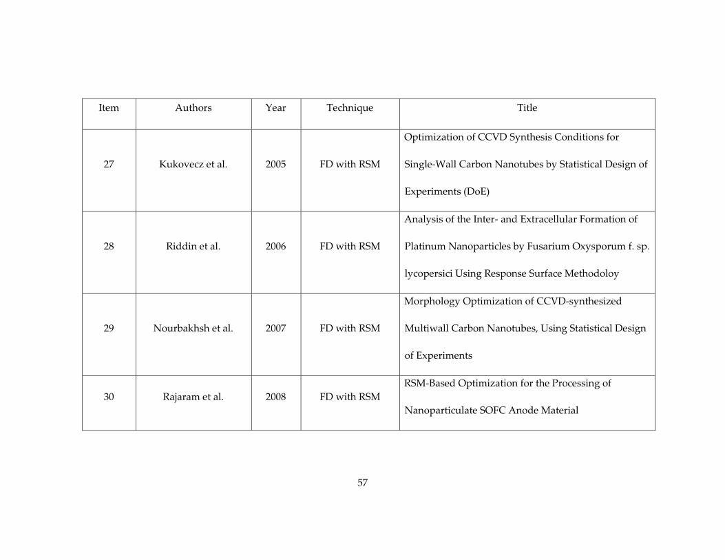
57
Item Authors Year Technique Title
27 Kukovecz et al. 2005 FD with RSM
Optimization of CCVD Synthesis Conditions for
Single-Wall Carbon Nanotubes by Statistical Design of
Experiments (DoE)
28 Riddin et al. 2006 FD with RSM
Analysis of the Inter- and Extracellular Formation of
Platinum Nanoparticles by Fusarium Oxysporum f. sp.
lycopersici Using Response Surface Methodoloy
29 Nourbakhsh et al. 2007 FD with RSM
Morphology Optimization of CCVD-synthesized
Multiwall Carbon Nanotubes, Using Statistical Design
of Experiments
30 Rajaram et al. 2008 FD with RSM
RSM-Based Optimization for the Processing of
Nanoparticulate SOFC Anode Material
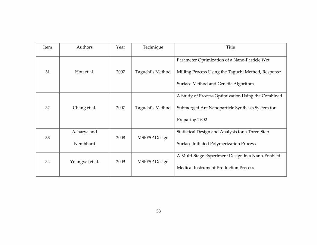
58
Item Authors Year Technique Title
31 Hou et al. 2007 Taguchi’s Method
Parameter Optimization of a Nano-Particle Wet
Milling Process Using the Taguchi Method, Response
Surface Method and Genetic Algorithm
32 Chang et al. 2007 Taguchi’s Method
A Study of Process Optimization Using the Combined
Submerged Arc Nanoparticle Synthesis System for
Preparing TiO2
33
Acharya and
Nembhard
2008 MSFFSP Design
Statistical Design and Analysis for a Three-Step
Surface Initiated Polymerization Process
34 Yuangyai et al. 2009 MSFFSP Design
A Multi-Stage Experiment Design in a Nano-Enabled
Medical Instrument Production Process
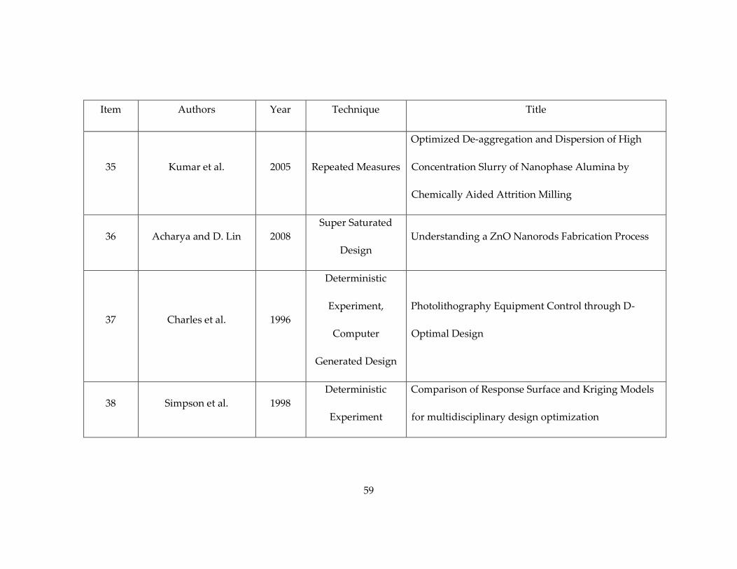
59
Item Authors Year Technique Title
35 Kumar et al. 2005 Repeated Measures
Optimized De-aggregation and Dispersion of High
Concentration Slurry of Nanophase Alumina by
Chemically Aided Attrition Milling
36 Acharya and D. Lin 2008
Super Saturated
Design
Understanding a ZnO Nanorods Fabrication Process
37 Charles et al. 1996
Deterministic
Experiment,
Computer
Generated Design
Photolithography Equipment Control through D-
Optimal Design
38 Simpson et al. 1998
Deterministic
Experiment
Comparison of Response Surface and Kriging Models
for multidisciplinary design optimization

60
Item Authors Year Technique Title
39 Cappelleri et al. 2002
Deterministic
Experiment
Design of a PZT Bimorph Actuator Using a
Metamodel-Based Approach
40 Aguirre et al. 2008
Deterministic
Experiment
A Framework for DOE and Deterministic Simulation
in Nano-Enabled Surgical Instrument Design
41 Hooker et al. 2003
Computer
Generated Design
An Evaluation of Population D-Optimal Designs Via
Pharmacokinetic Simulation
42 Chuang et al. 2004
Computer
Generated Design
Optimal Designs for Microarray Experiments

61
2.7 Remarks
Nanotechnology is becoming a key driver in economic growth around the globe
(Nembhard, 2007). It is also a highly multidisciplinary and integrates many areas science
and engineering. The impact of nanotechnology extends to advanced materials science,
manufacturing, energy and environment preservation, medicine, and others.
Corresponding with the rapid growth of nanotechnology, there has been
growing concern over how these technologies will be properly employed. If employed
incorrectly, this will eventually lead to a negative impact to humanity and the
environment. To help in understanding of using DOE in nanotechnology areas, much of
the content of this chapter has been published in Yuangyai and Nembhard (2009)
Several organizations have announced intentions or preparations for product
certification and standards for nanotechnology (Nembhard, 2007). In particular, the
International Organization for Standardization (ISO) is focused on developing and
promoting standards for using nanotechnology. Within ISO, three working groups are
considering proper terminology and nomenclature, measurement and characterization,
as well as health, safety, and environmental aspects of nanotechnologies .
The nanotechnology research and development community will be compelled to
make adjustments to adhere to these standards as well as ensure customer satisfaction.
DOE is an important tool that can help to fulfill both customer and industry needs
effectively and efficiently.

62
Chapter 3.
Multistage Fractional Factorial Split-Plot Designs
Our objective in this chapter is to develop a multistage fractional factorial split -
plot (MSFFSP) design that is primarily used for factor screening and for process
optimization. The design is applied to improve the manufacturability of the lost mold
rapid infiltration forming (LMRIF) process that was originally proposed by Antolino et
al. (2009a, 2009b).
The organization of this chapter is as follows. Section 3.1 describes the yield
improvement for LMRIF process. The choice of design associated with the LMRIF
process is discussed in Section 3.2. The topics related to split-plot design and its variants
as well as the procedure to MSFFSP design are reviewed and presented in Section 3.3,
followed by the derivation of linear model and its analysis in Section 3.4. The MSFFSP
design experimentation, results, analysis and conclusion is given in Section 3.5. Finally,
Section 3.6 provides concluding remarks.
3.1 Yield Improvement for LMRIF Process
This process was originally intended to fabricate micro surgical instruments that
are used for minimally invasive surgery (MIS). However, unsuccessful fabrication trials
made it clear that the initial process could not reliably fabricate components suitable for

63
surgical applications. Functional surgical instruments require larger lengths and cross-
sections than reported by Antolino et al. (2009a, 2009b) in order to withstand the forces
needed to perform surgical actions. Aspect ratios of 17:1 are standard for, according to
ASTM (2002), three point bend bars; however, surgical instrument designs require larger
aspect ratios to withstand the deformation and force used in surgery. Aguirre et al.
(2008b) show that 400 microns thick parts with an aspect ratio of at least 35:1 are feasible
dimensions for surgical instruments. Therefore, it is necessary to improve the process to
fabricate such parts for surgical instruments by increasing the dimensions.
Specific process changes and additions were incorporated into the LMRIF
process in order to fabricate the desired parts. First, a binder and plasticizer system was
added to the slurry formulation to improve strength of the green ceramic body so that it
will survive the stresses that arise during drying. Second, a solvent exchange drying
technique was instituted. The water in the gelled wet parts is displaced by ethanol to
minimize drying stresses due to solvent surface tension and reduce capillary forces in
the pore structure of the large cross sections. Last, a silicone mold release layer was
applied to the mold prior to infiltration to minimize part to mold wall adhesion. These
new modifications were the main focus of this DOE study.
The objective of this study is to understand how each of the five factors identified
in Table 3-1 affects the process yield. The factors and levels were chosen in consultation
with the scientists who developed the process. Note that we alternate between the use of
capital letters and small letters to distinguish the factors among stages. Also note that

64
stage 2 and stage 3 are both in the colloid deposition process.
Table 3-1. Factors of interest.
Process Stage Factors of interest
Levels
Low(-1) High(+1)
Powder
preparation
1: Powder
preparation
𝐴 Binder volume (%) 8 10
𝐵 Solid volume (%) 35 40
𝐶 Binder ratio
(PEG:PVA)
1:1 1:1.5
Colloid
deposition
2: Forming 𝑑 Surface coating No Yes
3: Immersing 𝐸 Immersion solution Ethanol Toluene
3.2 Choice of Design
There are many types of designs that can be used for this experimentation. To
understand the implications in choosing these designs, we first demonstrate the
different arrangements of the CR design, split-plot design, and split block design. Let us
consider only two sub processes – gel-casting and immersing, as in Figure 3-1. We will
assume that in the gel-casting process there are two factors of interest – percent of binder
volume (𝐴) and solid volume (𝐵) – and that each factor has two levels. In the colloid
deposition process (only the immersing stage is considered), there is one factor of
interest –the type of immersing chemical (𝐸) – and this factor has two levels. The

65
response (𝑦) is the green-state yield.
If a CR design is used, eight samples are prepared at different times, and each
sample must be placed into a furnace at different times (see Figure 3-2a). If the split-plot
design is used, there are only four sample preparations required. Each sample is split
into two sub-samples. Then each sub-sample is placed into the immersing bath at a
different time. Therefore, there are four sample preparations and eight immersing
settings (see Figure 3-2b).
In the split-block design, only four samples are prepared. Each is split into two
sub-samples, similar to those in split-plot design. However, these sub-samples are then
regrouped and placed into the bath at the low level or the high level together. This
reduces the sintering settings from eight to only two (Figure 3-2c).
Figure 3-1. Two stage process.
Gel Casting ImmersingA
E
BResponse Y

66
Figure 3-2. CR, split-plot, and split-block design arrangements.
3.3 MSFFSP Design with Three-stage Experimentation
Let us reconsider the three stage problem with five factors and similarly analyze
our position. Table 3-2 shows that the CR design requires a total of 25 = 32 runs, which
means 32 settings for all factors in each stage are required. When the multistage split-
plot (MSSP) design is used, both split-plot and split-block arrangement, the number of
settings is reduced. In particular, the split-block arrangement for all stages provides the
lowest number of settings which is equal to the number of treatment combinations
applied to experimental units at each stage. Note, however, that the number of runs
remains at 32.
The simplest way to reduce the number of runs is to conduct the experiment

67
under the fractional factorial (FF) design. Assuming, for example, a 1/4 fraction, the
number of runs would be decreased from 32 to 25-2 = 8, as shown in Table 3-2. However,
this design still requires the ability to completely randomize all the treatment
combinations.
Table 3-2. Number of settings and number of runs in CR, FF, and MSSP design.
Design
Number of settings in
Number of
runs
Stage 1:
Powder
preparation
Stage 2:
Forming
Stage 3:
Immersing
CR 32 32 32 32
MSSP
(23𝑥21𝑥21)
Split-Plot 8 16 32 32
Split-Block 8 2 2 32
FF (25−2) 8 8 8 8
In this research, it was recognized that in some situations it is not practical to
directly employ the split-plot or split-block structure. For example, it is practical to
perform experiments from stage 1 through stage 2 (particle preparation through mold
surface coating) and then regroup experimental units in the immersing process at
different immersing solutions. If regrouping is done after stage 1 (particle preparation),
all experiment units after this stage have to be filled in the same substrates which is
physically impossible. The combination of split-plot and split-block structure with the

68
MSFFSP design will be the most efficient and effective design under such constraints. In
our application, it is preferable that experimentation for stage 1 and 2 is performed with
the split-plot structure but stage 3 is performed with the split-block structure.
Given an experimental ‚budget‛ of 8 runs, we would have to rely on a fractional
factorial design. Therefore, it is important to review some recent methods of factor
confounding in multistage experiments suggested by Bisgaard (2000). Based on the
existing literature, we show the factor confounding using the two-stage FFSP designs for
stages 1 and 2 which involve factors 𝐴,𝐵,𝐶, and 𝑑 in Table 3-3. This design can be
represented by a 3 1 12 2 FFSP design.
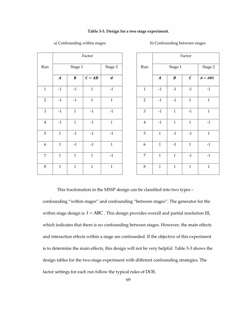
69
Table 3-3. Design for a two stage experiment.
a) Confounding within stages b) Confounding between stages
Run
Factor
Run
Factor
Stage 1 Stage 2 Stage 1 Stage 2
𝑨 𝑩 𝑪 = 𝑨𝑩 𝒅 𝑨 𝑩 𝑪 𝒅 = 𝑨𝑩𝑪
1 -1 -1 1 -1 1 -1 -1 -1 -1
2 -1 -1 1 1 2 -1 -1 1 1
3 -1 1 -1 -1 3 -1 1 -1 1
4 -1 1 -1 1 4 -1 1 1 -1
5 1 -1 -1 -1 5 1 -1 -1 1
6 1 -1 -1 1 6 1 -1 1 -1
7 1 1 1 -1 7 1 1 -1 -1
8 1 1 1 1 8 1 1 1 1
This fractionation in the MSSP design can be classified into two types –
confounding ‚within stages‛ and confounding ‚between stages‛. The generator for the
within stage design is . This design provides overall and partial resolution III,
which indicates that there is no confounding between stages. However, the main effects
and interaction effects within a stage are confounded. If the objective of this experiment
is to determine the main effects, this design will not be very helpful. Table 3-3 shows the
design tables for the two-stage experiment with different confounding strategies. The
factor settings for each run follow the typical rules of DOE.
I ABC

70
On the other hand, in order to maintain the highest resolution of the design, the
fractionation in each stage could be confounded between stages with the highest
interaction effect of other stage factors. Its design generator is . This design
provides an overall resolution IV which indicates the main effects are not confounded
with any second order interaction.
However, in this experimentation, if we employ the between stage confounding
factor, for example I=ABd=BCE=ACdE, the split-plot structure of the experimentation
will be destroyed. This destruction means eight particle preparations are required,
which after discussing with the manufacturing scientists was deemed experimentally
impractical. Therefore, we decided to use I=ABC=BdE=ACdE. This generator provides a
resolution III design as shown in Table 3-4. The design format is shown in Table 3-5.
Table 3-4. Factor confounding.
I=ABC=BdE=ACdE
A+BC+CdE+ABdE
B+AC+dE+ABCdE
C+AB+AdE+BCdE
d+BE+ACE+ABCd
E+Bd+ACd+ABCE
Ad+CE+ABE+BCd
AE+Cd+ABd+BCE
I ABCD
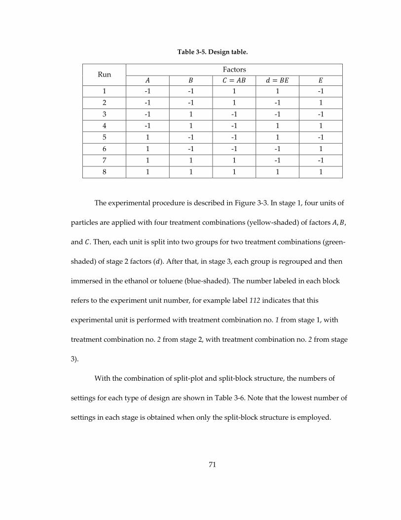
71
Table 3-5. Design table.
Run Factors
𝐴 𝐵 𝐶 = 𝐴𝐵 𝑑 = 𝐵𝐸 𝐸
1 -1 -1 1 1 -1
2 -1 -1 1 -1 1
3 -1 1 -1 -1 -1
4 -1 1 -1 1 1
5 1 -1 -1 1 -1
6 1 -1 -1 -1 1
7 1 1 1 -1 -1
8 1 1 1 1 1
The experimental procedure is described in Figure 3-3. In stage 1, four units of
particles are applied with four treatment combinations (yellow-shaded) of factors 𝐴,𝐵,
and 𝐶. Then, each unit is split into two groups for two treatment combinations (green-
shaded) of stage 2 factors (𝑑). After that, in stage 3, each group is regrouped and then
immersed in the ethanol or toluene (blue-shaded). The number labeled in each block
refers to the experiment unit number, for example label 112 indicates that this
experimental unit is performed with treatment combination no. 1 from stage 1, with
treatment combination no. 2 from stage 2, with treatment combination no. 2 from stage
3).
With the combination of split-plot and split-block structure, the numbers of
settings for each type of design are shown in Table 3-6. Note that the lowest number of
settings in each stage is obtained when only the split-block structure is employed.
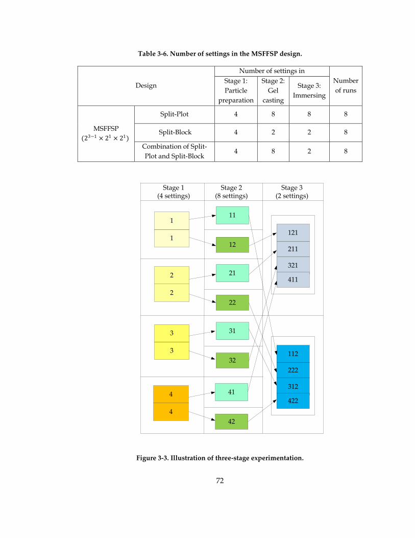
72
Table 3-6. Number of settings in the MSFFSP design.
Design
Number of settings in
Number
of runs
Stage 1:
Particle
preparation
Stage 2:
Gel
casting
Stage 3:
Immersing
MSFFSP
(23−1 × 21 × 21)
Split-Plot 4 8 8 8
Split-Block 4 2 2 8
Combination of Split-
Plot and Split-Block 4 8 2 8
11
121
1
Stage 1(4 settings)
Stage 2(8 settings)
21
22
2
2
31
32
3
3
41
42
4
4
Stage 3(2 settings)
121
211
321
411
112
222
312
422
Figure 3-3. Illustration of three-stage experimentation.

73
3.4 Linear Model of the Three stage Split-Plot Design and Its
Derivation
3.4.1 Derivation
As we know that in some situations, it is more convenient for the experimenters
to perform the experiment with the combination of split-plot and split block structure. In
this section, we derive the linear model for the experiment. In addition, Hinkelmann and
Kempthrone (2008) provide the derivation for the split-plot and split-block structure.
Paniagua-Quinones (2004) also shows a similar direction of the derivation of a split-
split-block structure. The derivation for a three-stage experiment with the combination
structure is extended from these earlier works.
The structure involves the split-plot structure in stage 1 and 2 and the split block
structure in stage 3. Let us assume there are 𝑗 (𝑗 = 1, . . ,𝑎) experiment treatment in stage
1, 𝑘 (𝑘 = 1, . . , 𝑏) experiment treatment in stage 2, and l (𝑙 = 1,… , 𝑐) in stage 3. The
conceptual unknown response is a constant value. If the experimental units have
contribution 𝑈𝑖𝑢𝑣𝑤 in the 𝑖𝑡 replicate, where 𝑢, 𝑣, and 𝑤 are the first stage, second stage,
and third stage identification numbers, and the response of treatment combination 𝑗𝑘𝑙
on this experimental unit, 𝑥𝑖𝑢𝑣𝑤𝑗𝑘𝑙 is displayed as
𝑥𝑖𝑢𝑣𝑤𝑗𝑘𝑙 = 𝑈𝑖𝑢𝑣𝑤 + 𝑇𝑗𝑘𝑙 (3-1)
where 𝑇𝑗𝑘𝑙 is the treatment contribution, then 𝑈𝑖𝑢𝑣𝑤 is the unit contribution due to

74
restriction on randomization and it can be written further as
𝑈𝑖𝑢𝑣𝑤 = 𝑈 … + 𝑈 𝑖 .. − 𝑈 .… + 𝑈 𝑖𝑢 .. − 𝑈 𝑖… + 𝑈 𝑖 .𝑣.. − 𝑈 𝑖… + 𝑈 𝑖 ..𝑤 − 𝑈 .…
+ 𝑈 𝑖𝑢 .𝑤 − 𝑈 𝑖𝑢 .. − 𝑈 𝑖𝑤 .. + 𝑈 𝑖… + 𝑈 𝑖 .𝑣𝑤 − 𝑈 𝑖 ..𝑣 − 𝑈 𝑖 ..𝑤 + 𝑈 𝑖…
+ 𝑈 𝑖𝑢𝑣𝑤 − 𝑈 𝑖𝑢𝑣 . − 𝑈 𝑖𝑢 .𝑤 − 𝑈 𝑖 ..𝑣𝑤 + 𝑈 𝑖𝑢 .. + 𝑈 𝑖 .𝑣. + 𝑈 𝑖 ..𝑤 − 𝑈 𝑖…
(3-2)
and
𝑇𝑗𝑘𝑙 = 𝑇 … + 𝑇 𝑗 .. − 𝑇 .… + 𝑇 .𝑘 .−𝑇 … + 𝑇 ..𝑙 − 𝑇 .… + 𝑇 𝑗𝑘 . − 𝑇 𝑗 .. − 𝑇 .𝑘. + 𝑇 …
+ 𝑇 𝑗 .𝑙 − 𝑇 𝑗 .. − 𝑇 ..𝑙 + 𝑇 … + 𝑇 .𝑘𝑙 − 𝑇 .𝑘 . − 𝑇 ..𝑙 + 𝑇 …
+ 𝑇 𝑗𝑘𝑙 − 𝑇 𝑗𝑘 . − 𝑇 𝑗 .𝑙 − 𝑇 .𝑘𝑙 + 𝑇 𝑗 .. + 𝑇 .𝑘 . + 𝑇 ..𝑙 − 𝑇 …
(3-3)
The overall mean is
𝜇 = 𝑈 …. + 𝑇 ...
The effect of the 𝑖𝑡 replicate is
𝜌𝑖 = 𝑈 𝑖… + 𝑈 ....
The effect of the 𝑗𝑡 first-stage treatment is
𝛼𝑗 = 𝑇 𝑗 .. + 𝑇 ...
The effect of the 𝑘𝑡 second-stage treatment is
𝛽𝑗 = 𝑇 .𝑘. + 𝑇 ...
The effect of the 𝑙𝑡 third-stage treatment is
𝛾𝑗 = 𝑇 ..𝑙 + 𝑇 ...
The interaction effect of the 𝑗𝑡 first-stage treatment and the 𝑘𝑡 second-stage treatment
is
𝛼𝛽𝑗𝑘 = 𝑇 𝑗𝑘 . − 𝑇 𝑗 .. − 𝑇 .𝑘 . + 𝑇 …
The interaction effect of the 𝑗𝑡 first-stage treatment and the 𝑙𝑡 third-stage treatment is
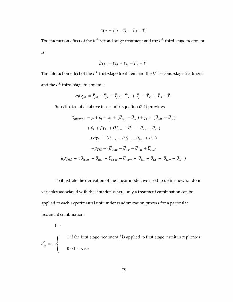
75
𝛼𝛾𝑗𝑙 = 𝑇 𝑗 .𝑙 − 𝑇 𝑗 .. − 𝑇 ..𝑙 + 𝑇 …
The interaction effect of the 𝑘𝑡 second-stage treatment and the 𝑙𝑡 third-stage treatment
is
𝛽𝛾𝑘𝑙 = 𝑇 .𝑘𝑙 − 𝑇 .𝑘. − 𝑇 ..𝑙 + 𝑇 …
The interaction effect of the 𝑗𝑡 first-stage treatment and the 𝑘𝑡 second-stage treatment
and the 𝑙𝑡 third-stage treatment is
𝛼𝛽𝛾𝑗𝑘𝑙 = 𝑇 𝑗𝑘𝑙 − 𝑇 𝑗𝑘 . − 𝑇 𝑗 .𝑙 − 𝑇 .𝑘𝑙 + 𝑇 𝑗 .. + 𝑇 .𝑘. + 𝑇 ..𝑙 − 𝑇 …
Substitution of all above terms into Equation (3-1) provides
𝑋𝑖𝑢𝑣𝑤𝑗𝑘𝑙 = 𝜇 + 𝜌𝑖 + 𝛼𝑗 + 𝑈 𝑖𝑢 .. − 𝑈 𝑖… + 𝛾𝑙 + 𝑈 𝑖 ..𝑤 − 𝑈 .…
+ 𝛽𝑘 + 𝛽𝛾𝑘𝑙 + 𝑈 𝑖𝑢𝑣 . −𝑈 𝑖𝑢 .. − 𝑈 𝑖 .𝑣. + 𝑈 𝑖…
+𝛼𝛾𝑗𝑙 + 𝑈 𝑖𝑢 .𝑤 − 𝑈 𝑓𝑖𝑢 .. − 𝑈 𝑖𝑤 .. + 𝑈 𝑖…
+𝛽𝛾𝑘𝑙 + 𝑈 𝑖 .𝑣𝑤 −𝑈 𝑖 ..𝑣 −𝑈 𝑖 ..𝑤 + 𝑈 𝑖…
𝛼𝛽𝛾𝑗𝑘𝑙 + 𝑈 𝑖𝑢𝑣𝑤 − 𝑈 𝑖𝑢𝑣 . − 𝑈 𝑖𝑢 .𝑤 − 𝑈 𝑖 ..𝑣𝑤 + 𝑈 𝑖𝑢 .. + 𝑈 𝑖 .𝑣. + 𝑈 𝑖 ..𝑤 − 𝑈 𝑖…
To illustrate the derivation of the linear model, we need to define new random
variables associated with the situation where only a treatment combination can be
applied to each experimental unit under randomization process for a particular
treatment combination.
Let
𝛿𝑖𝑢𝑗
=
1 if the first-stage treatment 𝑗 is applied to first-stage 𝑢 unit in replicate 𝑖
0 otherwise

76
𝛿𝑖𝑣𝑘 =
1 if the second-stage treatment 𝑘 is applied to first-stage 𝑣 unit in replicate 𝑖
0 otherwise
𝛿𝑖𝑤𝑙 =
1 if the third-stage treatment l is applied to first-stage 𝑤 unit in replicate 𝑖
0 otherwise
Then, letting 𝑎 be the number of the first-stage unit, 𝑏 be the number of second-
stage units, and 𝑐 be the number of third stage units. Note that, 𝛿𝑖𝑢𝑙 , 𝛿𝑖𝑣
𝑙 , and 𝛿𝑖𝑤𝑙 are
simply distributed as Bernoulli (0, 1). Then,
𝑃 𝛿𝑖𝑢𝑗
= 1 =1
𝑎 ,
𝑃 𝛿𝑖𝑢𝑗
= 1, 𝛿𝑖𝑢 ′𝑗 ′
= 1 =1
𝑎(𝑎−1) , 𝑗 ≠ 𝑗′,𝑢 ≠ 𝑢′
𝑃 𝛿𝑖𝑢𝑗
= 1, 𝛿𝑖𝑢 ′𝑗 ′
= 1, 𝛿𝑖𝑢 ′′𝑗 ′′
= 1 =1
𝑎 𝑎−1 (𝑎−2) , 𝑗 ≠ 𝑗′ ≠ 𝑗′′,𝑢 ≠ 𝑢′ ≠ 𝑢′′
and so on;
𝑃 𝛿𝑖𝑣𝑘 = 1 =
1
𝑏 ,
𝑃 𝛿𝑖𝑣𝑘 = 1, 𝛿
𝑖𝑣′𝑘 ′
= 1 =1
𝑏(𝑏−1) , 𝑘 ≠ 𝑘′,𝑣 ≠ 𝑣′
𝑃 𝛿𝑖𝑣𝑘 = 1, 𝛿
𝑖𝑣′𝑘 ′
= 1,𝛿𝑖𝑤𝑣 ′′𝑘 ′′
= 1 =1
𝑏 𝑏−1 (𝑏−2) , 𝑘 ≠ 𝑘′ ≠ 𝑘′′,𝑣 ≠ 𝑣′ ≠ 𝑣′′
and so on;
𝑃 𝛿𝑖𝑤𝑙 = 1 =
1
𝑐 ,
𝑃 𝛿𝑖𝑤𝑙 = 1, 𝛿
𝑖𝑤 ′𝑙′ = 1 =
1
𝑐(𝑐−1) , 𝑗 ≠ 𝑗′,𝑤 ≠ 𝑤′
𝑃 𝛿𝑖𝑤𝑗
= 1, 𝛿𝑖𝑤 ′𝑗 ′
= 1, 𝛿𝑖𝑤 ′′𝑗 ′′
= 1 =1
𝑐 𝑐−1 𝑐−2 , 𝑙 ≠ 𝑙′ ≠ 𝑙′′,𝑤 ≠ 𝑤′ ≠ 𝑤′′
and so on;

77
Let
𝜖𝑖𝑗𝑠1 = 𝛿𝑖𝑢
𝑗𝑎𝑢=1 𝑈 𝑖𝑢 .. − 𝑈 𝑖…
𝜖𝑖𝑗𝑘𝑠1&𝑠2 = 𝛿𝑖𝑢
𝑗𝛿𝑖𝑣𝑘 𝑈 𝑖𝑢𝑣 . −𝑈 𝑖𝑢 .. − 𝑈 𝑖 .𝑣. + 𝑈 𝑖…
𝑏𝑣=1
𝑎𝑢=1
𝜖𝑖𝑙𝑠3 = 𝛿𝑖𝑤
𝑙𝑐𝑤=1 𝑈 𝑖𝑤 .. − 𝑈 𝑖…
𝜖𝑖𝑗𝑙𝑠1&𝑠3 = 𝛿𝑖𝑢
𝑗𝛿𝑖𝑤𝑙 𝑈 𝑖𝑢 .𝑤 − 𝑈 𝑖𝑢 .. − 𝑈 𝑖 ..𝑤 + 𝑈 𝑖…
𝑐𝑤=1
𝑎𝑢=1
𝜖𝑖𝑘𝑙𝑠2&𝑠3 = 𝛿𝑖𝑣
𝑘 𝛿𝑖𝑤𝑙 𝑈 𝑖 .𝑣𝑤 − 𝑈 𝑖 .𝑣. − 𝑈 𝑖 .𝑤 . + 𝑈 𝑖…
𝑏𝑤=1
𝑏𝑣=1
𝜖𝑖𝑗𝑘𝑙𝑠1&𝑠2&𝑠3
= 𝛿𝑖𝑢𝑗𝑐
𝑤=1𝑏𝑣=1
𝑎𝑢=1 𝛿𝑖𝑣
𝑘 𝛿𝑖𝑤𝑙 (𝑈 𝑖𝑢𝑣𝑤 − 𝑈 𝑖𝑢𝑣 . − 𝑈 𝑖𝑢 .𝑤 − 𝑈 𝑖 ..𝑣𝑤 + 𝑈 𝑖𝑢 .. +
𝑈 𝑖 .𝑣. + 𝑈 𝑖 ..𝑤 − 𝑈 𝑖… )
The response 𝑦𝑖𝑗𝑘𝑙 of the 𝑗𝑘𝑙 treatment combination in replicate 𝑖 is observed
and connected to 𝑥𝑖𝑢𝑣𝑤𝑗𝑘𝑙 by three independent random variables (𝛿𝑖𝑢𝑙 , 𝛿𝑖𝑣
𝑙 , and 𝛿𝑖𝑤𝑙 ).
Then,
𝑌𝑖𝑗𝑘𝑙 = 𝛿𝑖𝑢𝑗𝑐
𝑤=1𝑏𝑣=1
𝑎𝑢=1 𝛿𝑖𝑣
𝑘 𝛿𝑖𝑤𝑙 𝑥𝑖𝑢𝑣𝑤𝑗𝑘𝑙
= 𝜇 + 𝜌𝑖 + 𝛼𝑗 + 𝜖𝑖𝑗𝑠1 + 𝛽𝑘 + 𝛼𝛽𝑗𝑘 + 𝜖𝑖𝑗𝑘
𝑠1&𝑠2 + 𝛾𝑙 + 𝜖𝑖𝑙𝑠3
+ 𝛼𝛾𝑗𝑙 + 𝜖𝑖𝑗𝑙𝑠1&𝑠3 + 𝛽𝛾𝑘𝑙 + 𝜖𝑖𝑘𝑙
𝑠2&𝑠3 + 𝛼𝛽𝛾𝑗𝑘𝑙 + 𝜖𝑖𝑗𝑘𝑙
𝑠1&𝑠2&𝑠3
The six error terms, generated from the randomization process of the three
stages, include 𝜖𝑖𝑗𝑠1 , 𝜖𝑖𝑗𝑘
𝑠1&𝑠2 , 𝜖𝑖𝑙𝑠3 , 𝜖𝑖𝑗𝑙
𝑠1&𝑠3 , 𝜖𝑖𝑘𝑙𝑠2&𝑠3 , and 𝜖𝑖𝑗𝑘𝑙
𝑠1&𝑠2&𝑠3 . Their distributional properties
are derived from 𝛿𝑖𝑢𝑗
, 𝛿𝑖𝑣𝑘 , and 𝛿𝑖𝑤
𝑗. Therefore, let us consider their properties:
𝐸 𝛿𝑖𝑢𝑗 =
1
𝑎 ,
𝑉𝑎𝑟 𝛿𝑖𝑢𝑗 = 𝐸 𝛿𝑖𝑢
𝑗
2− 𝐸 𝛿𝑖𝑢
𝑗
2=
1
𝑎−
1
𝑎
2=
1
𝑎 1 −
1
𝑎 , and
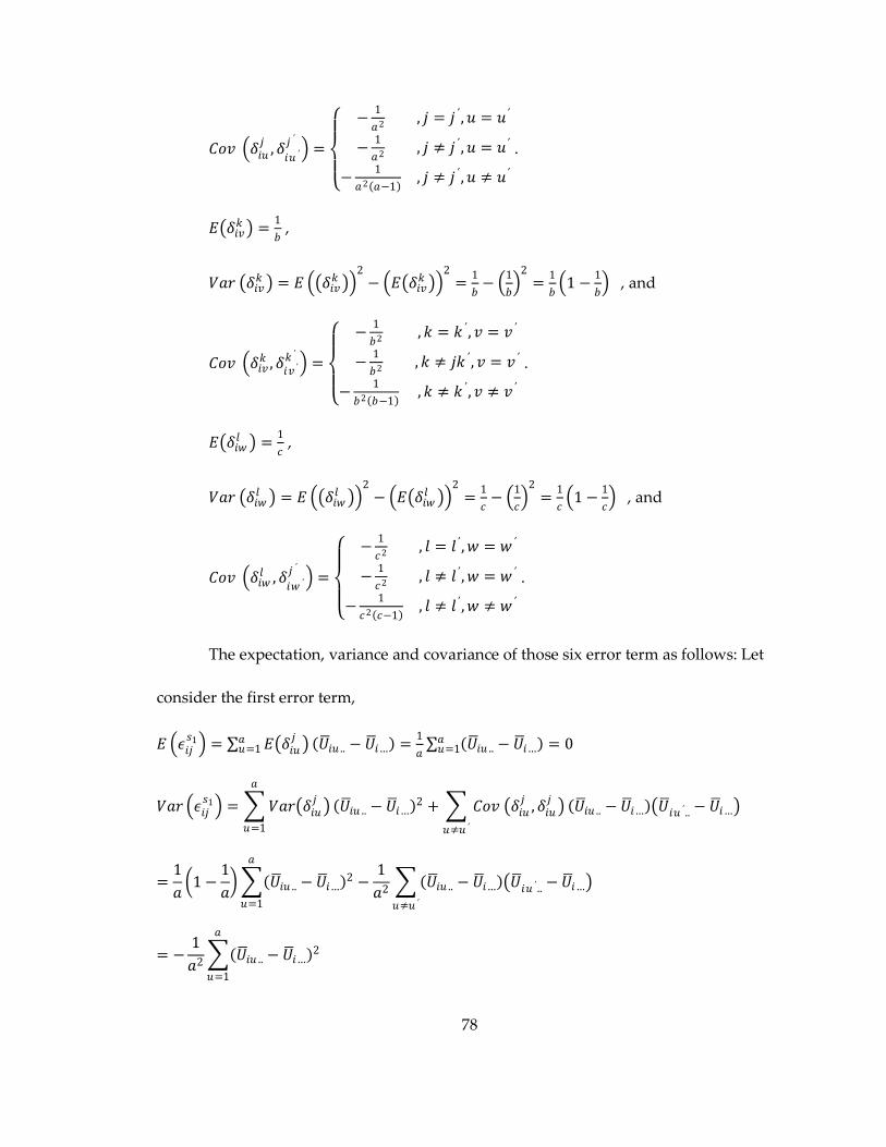
78
𝐶𝑜𝑣 𝛿𝑖𝑢𝑗
, 𝛿𝑖𝑢 ′𝑗 ′
=
−
1
𝑎2 , 𝑗 = 𝑗′,𝑢 = 𝑢′
−1
𝑎2 , 𝑗 ≠ 𝑗′,𝑢 = 𝑢′
−1
𝑎2 𝑎−1 , 𝑗 ≠ 𝑗′,𝑢 ≠ 𝑢′
.
𝐸 𝛿𝑖𝑣𝑘 =
1
𝑏 ,
𝑉𝑎𝑟 𝛿𝑖𝑣𝑘 = 𝐸 𝛿𝑖𝑣
𝑘 2− 𝐸 𝛿𝑖𝑣
𝑘 2
=1
𝑏−
1
𝑏
2=
1
𝑏 1 −
1
𝑏 , and
𝐶𝑜𝑣 𝛿𝑖𝑣𝑘 , 𝛿
𝑖𝑣′𝑘 ′ =
−
1
𝑏2 ,𝑘 = 𝑘′,𝑣 = 𝑣′
−1
𝑏2 ,𝑘 ≠ 𝑗𝑘′,𝑣 = 𝑣′
−1
𝑏2 𝑏−1 ,𝑘 ≠ 𝑘′,𝑣 ≠ 𝑣′
.
𝐸 𝛿𝑖𝑤𝑙 =
1
𝑐 ,
𝑉𝑎𝑟 𝛿𝑖𝑤𝑙 = 𝐸 𝛿𝑖𝑤
𝑙 2− 𝐸 𝛿𝑖𝑤
𝑙 2
=1
𝑐−
1
𝑐
2=
1
𝑐 1 −
1
𝑐 , and
𝐶𝑜𝑣 𝛿𝑖𝑤𝑙 , 𝛿
𝑖𝑤 ′𝑗 ′
=
−
1
𝑐2 , 𝑙 = 𝑙′,𝑤 = 𝑤′
−1
𝑐2 , 𝑙 ≠ 𝑙′,𝑤 = 𝑤′
−1
𝑐2 𝑐−1 , 𝑙 ≠ 𝑙′,𝑤 ≠ 𝑤′
.
The expectation, variance and covariance of those six error term as follows: Let
consider the first error term,
𝐸 𝜖𝑖𝑗𝑠1 = 𝐸 𝛿𝑖𝑢
𝑗 𝑎
𝑢=1 𝑈 𝑖𝑢 .. − 𝑈 𝑖… =1
𝑎 𝑈 𝑖𝑢 .. − 𝑈 𝑖… 𝑎𝑢=1 = 0
𝑉𝑎𝑟 𝜖𝑖𝑗𝑠1 = 𝑉𝑎𝑟 𝛿𝑖𝑢
𝑗
𝑎
𝑢=1
𝑈 𝑖𝑢 .. − 𝑈 𝑖… 2 + 𝐶𝑜𝑣 𝛿𝑖𝑢
𝑗, 𝛿𝑖𝑢
𝑗
𝑢≠𝑢 ′
𝑈 𝑖𝑢 .. − 𝑈 𝑖… 𝑈 𝑖𝑢 ′.. − 𝑈 𝑖…
=1
𝑎 1 −
1
𝑎 𝑈 𝑖𝑢 .. − 𝑈 𝑖…
2
𝑎
𝑢=1
−1
𝑎2 𝑈 𝑖𝑢 .. − 𝑈 𝑖… 𝑈 𝑖𝑢 ′.. −𝑈 𝑖…
𝑢≠𝑢 ′
= −1
𝑎2 𝑈 𝑖𝑢 .. − 𝑈 𝑖…
2
𝑎
𝑢=1

79
Since 𝑈 𝑖𝑢 .. − 𝑈 𝑖… 𝑈 𝑖𝑢 ′.. − 𝑈 𝑖… 𝑢≠𝑢 ′ = − 𝑈 𝑖𝑢 .. − 𝑈 𝑖… 2𝑎
𝑢=1 .
Let
𝜎𝑢2 =
1
𝑎−1 𝑈 𝑖𝑢 .. − 𝑈 𝑖…
2𝑎𝑢=1 ,
This allows us to write
𝑉𝑎𝑟 𝜖𝑖𝑗𝑠1 =
1
𝑎−1 𝜎𝑢
2.
We also find that for 𝑗 ≠ 𝑗′
𝐶𝑜𝑣 𝜖𝑖𝑗𝑠1 , 𝜖𝑖𝑗
𝑠1 = 𝐸(𝜖𝑖𝑗𝑠1𝜖
𝑖𝑗 ′𝑠1 ) − 𝐸 𝜖𝑖𝑗
𝑠1 𝐸 𝜖𝑖𝑗 ′𝑠1
= 𝐸 𝛿𝑖𝑢𝑗𝑎
𝑢=1 𝑈 𝑖𝑢 .. −𝑈 𝑖… 𝛿𝑖𝑢𝑗𝑎
𝑢=1 𝑈 𝑖𝑢 .. − 𝑈 𝑖…
= 𝐸 𝛿𝑖𝑢𝑗𝑎
𝑢≠𝑢 ′ 𝛿𝑖𝑢 ′𝑗 ′
𝑈 𝑖𝑢 .. −𝑈 𝑖… 𝑈 𝑖𝑢 ′.. − 𝑈 𝑖…
= 𝑈 𝑖𝑢 .. − 𝑈 𝑖… 𝑈 𝑖𝑢 ′.. − 𝑈 𝑖… 𝐸(𝑎𝑢≠𝑢 ′ 𝛿𝑖𝑢
𝑗𝛿𝑖𝑢 ′𝑗 ′
)
= 𝑈 𝑖𝑢 .. − 𝑈 𝑖… 𝑈 𝑖𝑢 ′.. − 𝑈 𝑖… (𝐶𝑜𝑣(𝑢≠𝑢 ′ 𝛿𝑖𝑢𝑗𝛿𝑖𝑢 ′𝑗 ′
) + 𝐸 𝛿𝑖𝑢𝑗 𝐸(𝛿
𝑖𝑢 ′𝑗 ′
))
= 𝑈 𝑖𝑢 .. − 𝑈 𝑖… 𝑈 𝑖𝑢 ′.. − 𝑈 𝑖… 1
𝑎2 𝑎−1 +
1
𝑎2 𝑢≠𝑢 ′
=1
𝑎 𝑎−1 𝑈 𝑖𝑢 .. − 𝑈 𝑖…
2𝑢≠𝑢 ′
= −𝜎𝑢
2
𝑎
Similarly, we can obtain the expectation, variance and covariance of the
remaining five error terms:
𝐸(𝜖𝑖𝑘𝑠1&𝑠2 ) = 0,
𝑉𝑎𝑟 𝜖𝑖𝑗𝑘𝑠1&𝑠2 = 1 −
1
𝑎𝑏 𝜎𝑢𝑣
2 , and
𝐶𝑜𝑣 𝜖𝑖𝑗𝑘𝑠1&𝑠2 , 𝜖𝑖𝑗𝑘
𝑠1&𝑠2 = −1
𝑎𝑏𝜎𝑢𝑣
2 ;
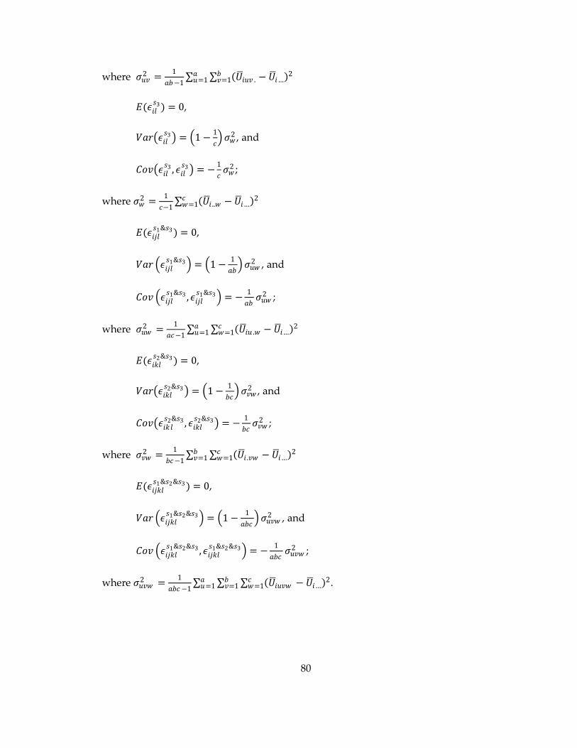
80
where 𝜎𝑢𝑣2 =
1
𝑎𝑏−1 𝑈 𝑖𝑢𝑣 . − 𝑈 𝑖…
2𝑏𝑣=1
𝑎𝑢=1
𝐸(𝜖𝑖𝑙𝑠3 ) = 0,
𝑉𝑎𝑟 𝜖𝑖𝑙𝑠3 = 1 −
1
𝑐 𝜎𝑤
2 , and
𝐶𝑜𝑣 𝜖𝑖𝑙𝑠3 , 𝜖𝑖𝑙
𝑠3 = −1
𝑐𝜎𝑤
2 ;
where 𝜎𝑤2 =
1
𝑐−1 𝑈 𝑖 ..𝑤 − 𝑈 𝑖…
2𝑐𝑤=1
𝐸(𝜖𝑖𝑗𝑙𝑠1&𝑠3 ) = 0,
𝑉𝑎𝑟 𝜖𝑖𝑗𝑙𝑠1&𝑠3 = 1 −
1
𝑎𝑏 𝜎𝑢𝑤
2 , and
𝐶𝑜𝑣 𝜖𝑖𝑗𝑙𝑠1&𝑠3 , 𝜖𝑖𝑗𝑙
𝑠1&𝑠3 = −1
𝑎𝑏𝜎𝑢𝑤
2 ;
where 𝜎𝑢𝑤2 =
1
𝑎𝑐−1 𝑈 𝑖𝑢 .𝑤 − 𝑈 𝑖…
2𝑐𝑤=1
𝑎𝑢=1
𝐸(𝜖𝑖𝑘𝑙𝑠2&𝑠3 ) = 0,
𝑉𝑎𝑟 𝜖𝑖𝑘𝑙𝑠2&𝑠3 = 1 −
1
𝑏𝑐 𝜎𝑣𝑤
2 , and
𝐶𝑜𝑣 𝜖𝑖𝑘𝑙𝑠2&𝑠3 , 𝜖𝑖𝑘𝑙
𝑠2&𝑠3 = −1
𝑏𝑐𝜎𝑣𝑤
2 ;
where 𝜎𝑣𝑤2 =
1
𝑏𝑐−1 𝑈 𝑖 .𝑣𝑤 − 𝑈 𝑖…
2𝑐𝑤=1
𝑏𝑣=1
𝐸(𝜖𝑖𝑗𝑘𝑙𝑠1&𝑠2&𝑠3 ) = 0,
𝑉𝑎𝑟 𝜖𝑖𝑗𝑘𝑙𝑠1&𝑠2&𝑠3 = 1 −
1
𝑎𝑏𝑐 𝜎𝑢𝑣𝑤
2 , and
𝐶𝑜𝑣 𝜖𝑖𝑗𝑘𝑙𝑠1&𝑠2&𝑠3 , 𝜖𝑖𝑗𝑘𝑙
𝑠1&𝑠2&𝑠3 = −1
𝑎𝑏𝑐𝜎𝑢𝑣𝑤
2 ;
where 𝜎𝑢𝑣𝑤2 =
1
𝑎𝑏𝑐 −1 𝑈 𝑖𝑢𝑣𝑤 − 𝑈 𝑖…
2𝑐𝑤=1
𝑏𝑣=1
𝑎𝑢=1 .

81
3.4.1.1 Linear Model and its assumptions
The linear model is useful to describe the observational data from an experiment.
In order to construct a linear model for the MSFFSP design, an understanding of the
linear models in the split-plot and split-block design is required; for the
experimentation, we employ a combination of split-plot structure in the first two stages
and split block structure in the last stage. Assuming that there are a levels of a stage 1
factor, b level of a stage 2 factor, c levels of stage 3, and n replicates, the linear model for
this design structure is
𝑦𝑔𝑖𝑗 = 𝜇 + 𝜌𝑔 + 𝛼 + 𝜖𝑔𝑠1 + 𝛽𝑖 + 𝛼𝛽𝑖 + 𝜖𝑔𝑖
𝑠1&𝑠2 + 𝛾𝑗 + 𝜖𝑔𝑖𝑠3
𝛼𝛾𝑗 + 𝜖𝑔𝑗𝑠1&𝑠3 + 𝛽𝛾𝑖𝑗 + 𝜖𝑔𝑖𝑗
𝑠2&𝑠3 + 𝛼𝛽𝛾𝑖𝑗 + 𝜖𝑔𝑖𝑗𝑠1&𝑠2&𝑠3
(3-4)
where
𝑦𝑔𝑖 is the 𝑔𝑖𝑗𝑡 response of the experiment,
𝜇 is a general overall mean effect,
𝜌𝑔 is the 𝑔𝑡 replicate effect 𝑁 0,𝜎𝜌2 ~𝑖𝑖𝑑,
𝛼 is the effect of gth level of stage 1 factor,
𝜖𝑔𝑠1 is the 𝑔𝑡 random error effect 𝑁 0,𝜎𝜖𝑠1
2 ~𝑖𝑖𝑑,
𝛽𝑖 is the effect of 𝑖𝑡 level of stage 2 factor,
𝛼𝛽 is the interaction effect of 𝑖𝑡 combination of stage 1 and 2 factor,
𝜖𝑔𝑖𝑠1&𝑠2 is the 𝑔𝑖𝑡 random error effect 𝑁 0,𝜎
𝜖𝑠1&𝑠22 ~𝑖𝑖𝑑,
𝛾𝑗 is the effect of 𝑗𝑡 level of stage 3 factor,

82
𝜖𝑔𝑗𝑠3 is the 𝑔𝑗𝑡 random error effect 𝑁 0,𝜎𝜖𝑠3
2 ~𝑖𝑖𝑑,
𝛼𝛾𝑗 is the interaction effect of 𝑗𝑡 combination of stage 1, and 3 factor,
𝜖𝑔𝑗𝑠1&𝑠3 is the 𝑔𝑗𝑡 random error effect 𝑁 0,𝜎
𝜖𝑠1&𝑠32 ~𝑖𝑖𝑑,
𝛽𝛾𝑖𝑗 is the interaction effect of 𝑖𝑗𝑡 combination of stage 2, and 3 factor,
𝜖𝑔𝑖𝑗𝑠2&𝑠3 is the 𝑔𝑖𝑗𝑡 random error effect 𝑁 0,𝜎
𝜖𝑠2&𝑠32 ~𝑖𝑖𝑑,
𝛼𝛽𝛾𝑖𝑗 is the interaction effect of 𝑖𝑗𝑡 combination of stage 1, 2, and 3 factor,
𝜖𝑔𝑖𝑗𝑠1&𝑠2&𝑠3 is the 𝑔𝑖𝑗𝑡 random error effect 𝑁 0,𝜎
𝜖𝑠1&𝑠2&𝑠32 ~𝑖𝑖𝑑.
All errors are mutually independent.
Note that the superscript of each error term indicates the stage number and its
interaction with factors from other stages, for example, is the error term due to
the interaction among factors from stage 1, stage 2 and stage 3.
The linear model in Equation (3-4) indicates that there are six error terms in total,
The first three error terms correspond to effects of the first three stage factors,
respectively. While the other three error terms correspond to interaction effects among
stage 1 and stage 2, stage 2 and stage 3 and stage 1, stage 2 and stage 3. It is important to
know which contrasts will be tested against which error term in order to test for
significance. In addition, this linear model is generalized and can also be used for the
MSSP design and the MSFFSP design with or without replication.
Note that this derivation is for a specific structure of MSFFSP design where the
first stage and the second stag experiment is conducted based on split plot structure and
split block structure for the second and the third stage. The different structure of
1 2 3s &s &s
ghij

83
experimentation can be simply extended from the linear model provided.
3.4.2 Analysis of the MSFFSP Design
3.4.2.1 Replicated MSSP Design
The derivation of variance component in the previous section leads to the
ANOVA given in Table 3-7 that we can use to test the significance of each main effect
and their interaction.
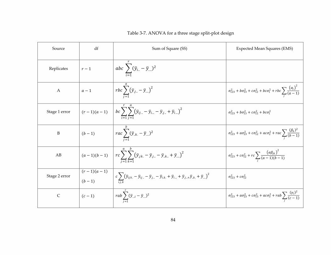
84
Table 3-7. ANOVA for a three stage split-plot design
Source df Sum of Square (SS) Expected Mean Squares (EMS)
Replicates 𝑟 − 1 𝑎𝑏𝑐 𝑦 𝑖 .. − 𝑦 .… 2
𝑟
𝑖=1
A 𝑎 − 1 𝑟𝑏𝑐 𝑦 .𝑗 .. − 𝑦 .… 2
𝑎
𝑗=1
𝜎1232 + 𝑏𝜎13
2 + 𝑐𝜎122 + 𝑏𝑐𝜎1
2 + 𝑟𝑏𝑐 𝛼𝑗
2
𝑎 − 1 𝑗
Stage 1 error (𝑟 − 1)(𝑎 − 1) 𝑏𝑐 𝑦 𝑖𝑗 .. − 𝑦 𝑖 ... − 𝑦 .𝑗 .. + 𝑦 𝑖… 2
𝑎
𝑗=1
𝑟
𝑖=1
𝜎1232 + 𝑏𝜎13
2 + 𝑐𝜎122 + 𝑏𝑐𝜎1
2
B (𝑏 − 1) 𝑟𝑎𝑐 𝑦 ..𝑘 . − 𝑦 .… 2
𝑏
𝑗=1
𝜎1232 + 𝑎𝜎23
2 + 𝑐𝜎122 + 𝑎𝑐𝜎2
2 + 𝑟𝑎𝑐 𝛽𝑘
2
𝑏 − 1 𝑗
AB (𝑎 − 1)(𝑏 − 1) 𝑟𝑐 𝑦 .𝑗𝑘 . − 𝑦 .𝑗 .. − 𝑦 ..𝑘 .. + 𝑦 .… 2
𝑏
𝑘=1
𝑎
𝑗=1
𝜎1232 + 𝑐𝜎12
2 + 𝑟𝑐 𝛼𝛽𝑗𝑘
2
𝑎 − 1 (𝑏 − 1)𝑗
Stage 2 error 𝑟 − 1 𝑎 − 1
(𝑏 − 1) 𝑐 𝑦 𝑖𝑗𝑘 . − 𝑦 𝑖𝑗 .. − 𝑦 .𝑗 .. − 𝑦 𝑖 .𝑘 . + 𝑦 𝑖… + 𝑦 .𝑗 ..+𝑦 ..𝑘 . + 𝑦 .…
2
𝑖 ,𝑗 ,𝑘
𝜎1232 + 𝑐𝜎12
2
C (𝑐 − 1) 𝑟𝑎𝑏 𝑦 …𝑙 − 𝑦 .… 2
𝑐
𝑗=1
𝜎1232 + 𝑎𝜎23
2 + 𝑐𝜎132 + 𝑎𝑐𝜎3
2 + 𝑟𝑎𝑏 𝛾𝑙
2
𝑐 − 1 𝑗

85
Source df Sum of Square (SS) Expected Mean Squares (EMS)
Stage 3 error (𝑟 − 1)(𝑐 − 1) 𝑎𝑏 𝑦 𝑖𝑗 .. − 𝑦 𝑖 ... − 𝑦 .𝑗 .. + 𝑦 𝑖… 2
𝑐
𝑘=1
𝑟
𝑗=1
𝜎1232 + 𝑎𝜎23
2 + 𝑏𝜎132 + 𝑎𝑏𝜎3
2
AC (𝑎 − 1)(𝑏 − 1) 𝑎𝑐 𝑦 .𝑗 .𝑙 − 𝑦 .𝑗 .. − 𝑦 ...𝑙 + 𝑦 .… 2
𝑏
𝑙=1
𝑟
𝑖=1
𝜎1232 + 𝑏𝜎13
2 + 𝑟𝑏 𝛼𝛾𝑘𝑙
2
𝑎 − 1 (𝑐 − 1)𝑗𝑘𝑙
Stage 1&3 error 𝑟 − 1 𝑎 − 1
(𝑐 − 1) 𝑏 𝑦 𝑖𝑗 .𝑙 − 𝑦 𝑖𝑗 .. − 𝑦 .𝑗 .. − 𝑦 𝑖 ..𝑙 + 𝑦 𝑖… + 𝑦 .𝑗 ..+𝑦 ...𝑙 + 𝑦 .…
2
𝑖 ,𝑗 ,𝑙
𝜎1232 + 𝑏𝜎13
2
BC (𝑏 − 1)(𝑐 − 1) 𝑏𝑐 𝑦 .𝑗𝑘 . − 𝑦 .𝑗 .. − 𝑦 ..𝑘 . + 𝑦 .… 2
𝑎
𝑗=1
𝑟
𝑖=1
𝜎1232 + +𝑎𝜎23
2 + 𝑟𝑎 𝛽𝛾𝑗𝑘𝑙
2
𝑏 − 1 (𝑐 − 1)𝑗𝑘𝑙
Stage 2&3 error 𝑟 − 1 𝑏 − 1
(𝑐 − 1) 𝑎 𝑦 𝑖 .𝑘𝑙 − 𝑦 𝑖 .𝑘 . − 𝑦 ..𝑘𝑙 − 𝑦 𝑖 ..𝑙 + 𝑦 𝑖… + 𝑦 .𝑗 ..+𝑦 ...𝑙 + 𝑦 .…
2
𝑖 ,𝑘 ,𝑙
𝜎1232 + 𝑎𝜎23
2
ABC 𝑎 − 1 𝑏 − 1
(𝑐 − 1) 𝑟 𝑦 .𝑗𝑘𝑙 − 𝑦 .𝑗𝑘 . − 𝑦 .𝑗 .𝑙 − 𝑦 ..𝑘𝑙 + 𝑦 ..𝑘 . + 𝑦 .𝑗 ..+𝑦 ...𝑙 + 𝑦 .…
2
𝑖 ,𝑗 ,𝑙
𝜎1232 + 𝑟
𝛼𝛽𝛾𝑗𝑘𝑙 2
𝑎 − 1 𝑏 − 1 (𝑐 − 1)𝑗𝑘𝑙
Stage 1&2&3 error 𝑟 − 1 𝑎 − 1
(𝑏 − 1)(𝑐 − 1) 𝑦𝑖𝑗𝑘𝑙 − 𝑦 𝑖𝑗 .. − 𝑦 𝑖 .𝑘 . − 𝑦 𝑖 ..𝑙 + 𝑦 𝑖… + 𝑦 .𝑗 .. + 𝑦 ...𝑘 . + 𝑦 ...𝑙 + 𝑦 .…
2
𝑖 ,𝑗 ,𝑘 ,𝑙
𝜎1232
Total rabc-1 𝑦𝑖𝑗𝑘𝑙 − 𝑦 .… 2
𝑖 ,𝑗 ,𝑘 ,𝑙

86
3.4.2.2 Unreplicated MSSP Design
In situations where we cannot replicate the design, the analysis without
replication is used. In this section, we will also show that how can we estimate standard
error of contrast of each effects. In this case, let us consider the situation where there is in
only 3 sets of factors: factor in stage 1, factor is stage 2 and factor is stage 3.
Table 3-8. Error terms for each response.
Run Factor Response Error term
𝐴 B C
1 −1 −1 −1 𝑦121 𝜖11 + 𝜖12
12 + 𝜖31 + 𝜖13
11 + 𝜖2321 + 𝜖123
121
2 −1 −1 1 𝑦112 𝜖11 + 𝜖12
11 + 𝜖32 + 𝜖13
12 + 𝜖2312 + 𝜖123
112
3 −1 1 −1 𝑦111 𝜖12 + 𝜖12
21 + 𝜖31 + 𝜖13
21 + 𝜖2311 + 𝜖123
211
4 −1 1 1 𝑦122 𝜖12 + 𝜖12
22 + 𝜖32 + 𝜖13
22 + 𝜖2322 + 𝜖123
222
5 1 −1 −1 𝑦221 𝜖13 + 𝜖12
32 + 𝜖31 + 𝜖13
31 + 𝜖2321 + 𝜖123
321
6 1 −1 1 𝑦212 𝜖13 + 𝜖12
31 + 𝜖32 + 𝜖13
32 + 𝜖2312 + 𝜖123
312
7 1 1 −1 𝑦211 𝜖14 + 𝜖12
41 + 𝜖31 + 𝜖13
41 + 𝜖2311 + 𝜖123
411
8 1 1 1 𝑦222 𝜖14 + 𝜖12
42 + 𝜖32 + 𝜖13
42 + 𝜖2322 + 𝜖123
422
The responses of an experiment are shown in Table 3-8. The estimate of any
effect is calculated by using the form 𝑦 (+1) − 𝑦 (−1). Let us assume that a fixed effects

87
model is considered, we need only focus on the error terms when calculating the
variance of the contrasts. To illustrate how to obtain the expression for the variance for
the variance of the contrast, let us consider the above experiment. The effect of 𝐴 is
written as
𝐴 =1
4 𝑦321 + 𝑦312 + 𝑦411 + 𝑦422 −
1
4(𝑦121 + 𝑦211 + 𝑦211 + 𝑦222 ),
𝑉𝑎𝑟 𝐴 =1
16{[(𝜖1
3 + 𝜖1232 + 𝜖3
1 + 𝜖1331 + 𝜖23
21 + 𝜖123312 ) + 𝜖1
3 + 𝜖1231 + 𝜖3
2 + 𝜖1332 + 𝜖23
12 + 𝜖123312 +
(𝜖14 + 𝜖12
41 + 𝜖31 + 𝜖13
41 + 𝜖2311 + 𝜖123
411 ) + (𝜖14 + 𝜖12
42 + 𝜖32 + 𝜖13
42 + 𝜖2322 + 𝜖123
422 )]
−[(𝜖11 + 𝜖12
12 + 𝜖31 + 𝜖13
11 + 𝜖2321 + 𝜖123
121 ) + ( 𝜖11 + 𝜖12
11 + 𝜖32 + 𝜖13
12 + 𝜖2312 + 𝜖123
112)+(𝜖12 + 𝜖12
21 +
𝜖31 + 𝜖13
21 + 𝜖2311 + 𝜖123
211 ) + (𝜖12 + 𝜖12
22 + 𝜖32 + 𝜖13
22 + 𝜖2322 + 𝜖123
222 )]}
=1
16𝑉𝑎𝑟 2𝜖1
3 + 2𝜖14 − 2𝜖1
1 − 2𝜖12
+1
16𝑉𝑎𝑟 𝜖12
32 + 𝜖1231 + 𝜖12
41 + 𝜖1242 − (𝜖12
12 + 𝜖1211 + 𝜖12
21 + 𝜖1222)
+1
16𝑉𝑎𝑟 𝜖3
1 + 𝜖32 + 𝜖3
1 + 𝜖32 − (𝜖3
1 + 𝜖32 + 𝜖3
1 + 𝜖32)
+1
16𝑉𝑎𝑟 𝜖13
31 + 𝜖1332 + 𝜖13
41 + 𝜖1342 − (𝜖13
11 + 𝜖1312 + 𝜖13
21 + 𝜖1322)
+1
16𝑉𝑎𝑟 𝜖23
21 + 𝜖2312 + 𝜖23
11 + 𝜖2322 − (𝜖23
21 + 𝜖2312 + 𝜖23
11 + 𝜖2322)
+1
16𝑉𝑎𝑟 𝜖123
321 + 𝜖123312 + 𝜖123
411 + 𝜖123422 − (𝜖123
121 + 𝜖123112 + 𝜖123
211 + 𝜖123222 )
= 1
16(16𝜎1
2 + 8𝜎122 + 8𝜎13
2 + 8𝜎1232 )
= 𝜎12 +
1
2𝜎12
2 +1
2𝜎13
2 +1
2𝜎123
2 .
Similarly,
𝑉𝑎𝑟 𝐵 = 1
2𝜎12
2 +1
2𝜎123
2 ,

88
𝑉𝑎𝑟 𝐴𝐵 = 1
2𝜎12
2 +1
2𝜎123
2 ,
𝑉𝑎𝑟 𝐶 = 𝜎132 +
1
2𝜎13
2 +1
2𝜎23
2 +1
2𝜎123
2 ,
𝑉𝑎𝑟 𝐴𝐶 = 1
2𝜎13
2 +1
2𝜎123
2 , and
𝑉𝑎𝑟 𝐴𝐵𝐶 = 1
2𝜎123
2 .
From the above derivation, it is clearly seen that each effect has different error
structure, which means different normal probability plots are required. The number of
plots can be determined from the linear model associated with how the experimentation
is performed.
3.4.2.3 Analysis of the MSFFSP Design
The analysis of the MSFFSP design is based on whether or not the design is
replicated. If the design is replicated, the ANOVA technique with difference errors
terms may be used; if not, the normal probability plot for appropriate effect might be
used. The disadvantage of MSFFSP analysis is that when there are several stages
involved in the experimentation, several errors terms need to be estimated and they
must be carefully chosen to be tested with effects. In addition, since the design is
fractionated, some information is lost and the errors may not be estimated, therefore, we
suggest the use of the remaining information as demonstrated in Section 3.5.

89
3.5 MSFFSP Design Implementation for LMRIF process
3.5.1 Implementation
In our experimentation, if the unreplicated design is used, Table 3-8 shows the
contrasts having the same error. However, since this is a fractionated design, some
contrasts are confounded with others, based on the generator. The effects must be
properly assigned to appropriate errors, as summarized in Table 3-9. Note that only
main effects and the second-order interactions are considered. Normal probability plots
are used to analyze the results. There are four plots required to test the significance of
effects 𝐴,𝐵,𝐶,𝑑,𝐴𝑑,𝐸 and 𝐴𝐸. However, there is an inefficient number of effects to
construct the plots because the maximum effect for each error term is three.
In order to overcome this situation, there are two possibilities: increase the level
of fractionation, or perform another replication. To increase the fractionation, a new
generator is required to create another eight runs with different treatment combinations.
After discussion with the project members, we decided to take the second approach and
replicate the design because this replication permits estimation of the experimental
errors and simplifies the analysis.
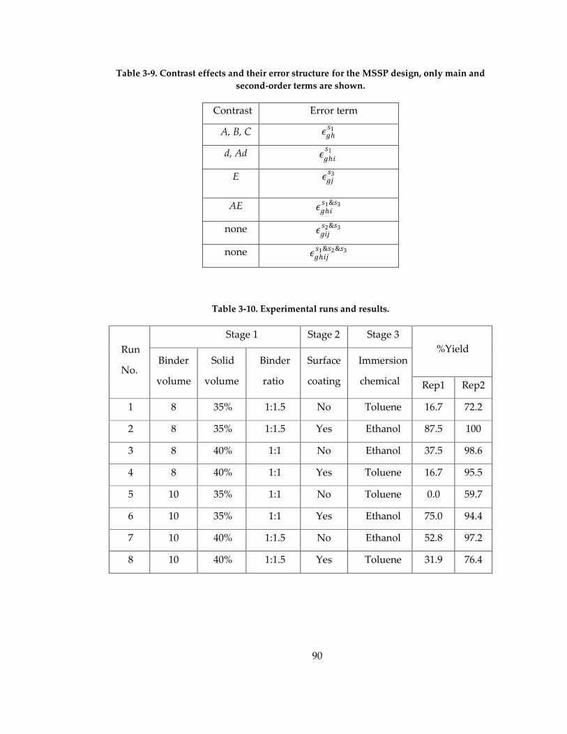
90
Table 3-9. Contrast effects and their error structure for the MSSP design, only main and
second-order terms are shown.
Contrast Error term
A, B, C 𝜖𝑔𝑠1
d, Ad 𝜖𝑔𝑖
𝑠1
E 𝜖𝑔𝑗𝑠3
AE 𝜖𝑔𝑖𝑠1&𝑠3
none 𝜖𝑔𝑖𝑗𝑠2&𝑠3
none 𝜖𝑔𝑖𝑗𝑠1&𝑠2&𝑠3
Table 3-10. Experimental runs and results.
Run
No.
Stage 1 Stage 2 Stage 3
%Yield Binder
volume
Solid
volume
Binder
ratio
Surface
coating
Immersion
chemical Rep1 Rep2
1 8 35% 1:1.5 No Toluene 16.7 72.2
2 8 35% 1:1.5 Yes Ethanol 87.5 100
3 8 40% 1:1 No Ethanol 37.5 98.6
4 8 40% 1:1 Yes Toluene 16.7 95.5
5 10 35% 1:1 No Toluene 0.0 59.7
6 10 35% 1:1 Yes Ethanol 75.0 94.4
7 10 40% 1:1.5 No Ethanol 52.8 97.2
8 10 40% 1:1.5 Yes Toluene 31.9 76.4

91
3.5.2 Results, Analysis and Discussion
The results of the experiment, shown in Table 3-10, were analyzed using Minitab
software (General Linear Model). All mean square errors have been calculated with
selected effects regrouped and reorganized with the associated error terms based on
Table 3-9.
In addition, we consider process yield as a response or output of experiment and
it may not be normally distributed. However, since ANOVA technique is used and the
F-test is robust to deviation from normality assumption (Box and Anderson, 1955).
Table 3-11 shows the reorganized ANOVA table. The effects of A, B, C are tested
with 𝜖𝑔𝑠1 (Error 1) derived from the summation of sum square errors of interaction of
factor A and replication, sum square errors of the interaction of factor B and replication,
as well as the sum square of interaction of factor C and replication. Due to the nature of
fractional design, the interaction of A, B, C and replication is not estimable. However, in
general, if the full factorial design is used, the effects of A, B, and C will be tested with
the interaction of A, B, C and replication.
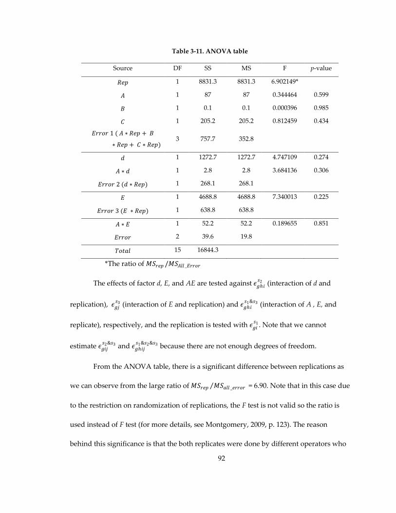
92
Table 3-11. ANOVA table
Source DF SS MS F p-value
𝑅𝑒𝑝 1 8831.3 8831.3 6.902149*
𝐴 1 87 87 0.344464 0.599
𝐵 1 0.1 0.1 0.000396 0.985
𝐶 1 205.2 205.2 0.812459 0.434
𝐸𝑟𝑟𝑜𝑟 1 ( 𝐴 ∗ 𝑅𝑒𝑝 + 𝐵
∗ 𝑅𝑒𝑝 + 𝐶 ∗ 𝑅𝑒𝑝) 3 757.7 352.8
𝑑 1 1272.7 1272.7 4.747109 0.274
𝐴 ∗ 𝑑 1 2.8 2.8 3.684136 0.306
𝐸𝑟𝑟𝑜𝑟 2 (𝑑 ∗ 𝑅𝑒𝑝) 1 268.1 268.1
𝐸 1 4688.8 4688.8 7.340013 0.225
𝐸𝑟𝑟𝑜𝑟 3 (𝐸 ∗ 𝑅𝑒𝑝) 1 638.8 638.8
𝐴 ∗ 𝐸 1 52.2 52.2 0.189655 0.851
𝐸𝑟𝑟𝑜𝑟 2 39.6 19.8
𝑇𝑜𝑡𝑎𝑙 15 16844.3
*The ratio of 𝑀𝑆𝑟𝑒𝑝 /𝑀𝑆𝐴𝑙𝑙 _𝐸𝑟𝑟𝑜𝑟
The effects of factor d, E, and AE are tested against 𝜖𝑔𝑖𝑠2 (interaction of d and
replication), 𝜖𝑔𝑗𝑠3 (interaction of E and replication) and 𝜖𝑔𝑖
𝑠1&𝑠3 (interaction of A , E, and
replicate), respectively, and the replication is tested with 𝜖𝑔𝑖𝑠1 . Note that we cannot
estimate 𝜖𝑔𝑖𝑗𝑠2&𝑠3 and 𝜖𝑔𝑖𝑗
𝑠1&𝑠2&𝑠3 because there are not enough degrees of freedom.
From the ANOVA table, there is a significant difference between replications as
we can observe from the large ratio of 𝑀𝑆𝑟𝑒𝑝 𝑀𝑆𝑎𝑙𝑙 _𝑒𝑟𝑟𝑜𝑟 = 6.90. Note that in this case due
to the restriction on randomization of replications, the F test is not valid so the ratio is
used instead of F test (for more details, see Montgomery, 2009, p. 123). The reason
behind this significance is that the both replicates were done by different operators who

93
have different skill levels in mold filling. The operator no. 2 (replication 2) outperforms
the operator no. 1 (replication 1). In order to improve the reproducibility of the process,
the scientists agree to investigate using an automatic filling machine, to eliminate human
error.
In addition, the type of immersing chemical (p-value = 0.225), as well as the mold
surface coating factor is significant (p-value = 0.274). Although these p-values are slightly
high compared to the general acceptance level (0.05 or 0.10), this level should not be
automatically used as a decision criteria without experimenters’ judgment (Box, Hunter,
and Hunter, 2005, p.188). In our case, we believe that this information combined with
our scientific knowledge of the LMRIF process is still valid for further improvement.
The immersing solution is used in the process because a solvent exchange drying
process is employed to minimize drying stress and improve yield. Water saturated,
gelled, green parts are placed into an ethanol bath for four hours, during which time a
solvent exchange takes place. After four hours, the parts are dried in the ambient
atmosphere. Ethanol was chosen because of its miscibility with water as well as a low
surface tension. The lower surface tension reduces the capillary drying stresses in the
porous parts and minimizes cracking.
A silicone mold surface coating was selected to ensure a non-wetting surface for
our aqueous based slurries, as well as provide lubrication between the green parts and
the mold walls. As the parts dry, they shrink away from the mold walls. If green parts
adhere to the mold walls, the part experiences increased stress during drying which may
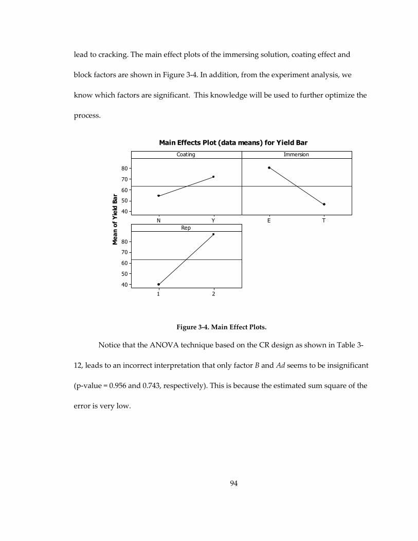
94
lead to cracking. The main effect plots of the immersing solution, coating effect and
block factors are shown in Figure 3-4. In addition, from the experiment analysis, we
know which factors are significant. This knowledge will be used to further optimize the
process. M
ea
n o
f Y
ield
Ba
r
YN
80
70
60
50
40
TE
21
80
70
60
50
40
Coating Immersion
Rep
Main Effects Plot (data means) for Yield Bar
Figure 3-4. Main Effect Plots.
Notice that the ANOVA technique based on the CR design as shown in Table 3-
12, leads to an incorrect interpretation that only factor B and Ad seems to be insignificant
(p-value = 0.956 and 0.743, respectively). This is because the estimated sum square of the
error is very low.
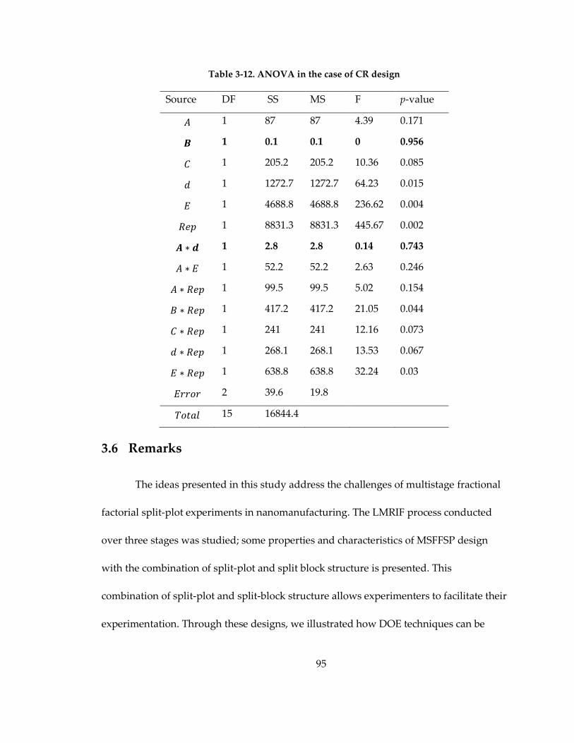
95
Table 3-12. ANOVA in the case of CR design
Source DF SS MS F p-value
𝐴 1 87 87 4.39 0.171
𝑩 1 0.1 0.1 0 0.956
𝐶 1 205.2 205.2 10.36 0.085
𝑑 1 1272.7 1272.7 64.23 0.015
𝐸 1 4688.8 4688.8 236.62 0.004
𝑅𝑒𝑝 1 8831.3 8831.3 445.67 0.002
𝑨 ∗ 𝒅 1 2.8 2.8 0.14 0.743
𝐴 ∗ 𝐸 1 52.2 52.2 2.63 0.246
𝐴 ∗ 𝑅𝑒𝑝 1 99.5 99.5 5.02 0.154
𝐵 ∗ 𝑅𝑒𝑝 1 417.2 417.2 21.05 0.044
𝐶 ∗ 𝑅𝑒𝑝 1 241 241 12.16 0.073
𝑑 ∗ 𝑅𝑒𝑝 1 268.1 268.1 13.53 0.067
𝐸 ∗ 𝑅𝑒𝑝 1 638.8 638.8 32.24 0.03
𝐸𝑟𝑟𝑜𝑟 2 39.6 19.8
𝑇𝑜𝑡𝑎𝑙 15 16844.4
3.6 Remarks
The ideas presented in this study address the challenges of multistage fractional
factorial split-plot experiments in nanomanufacturing. The LMRIF process conducted
over three stages was studied; some properties and characteristics of MSFFSP design
with the combination of split-plot and split block structure is presented. This
combination of split-plot and split-block structure allows experimenters to facilitate their
experimentation. Through these designs, we illustrated how DOE techniques can be

96
used in nanomanufacturing design and engineering by helping researchers understand
process dynamics. The work in this chapter has been presented in Yuangyai et al. (2009)
and Aguirre et al. (2009).

97
Chapter 4.
Optimal Multistage Fractional Factorial Split-Plot Design
In Chapter 3, we presented the idea of MSFFSP design with the combination of
split-plot and split-block and its derivation of a linear model as well as its analysis. The
design presented was based on the experimenter’s knowledge and interest. In this
chapter, we will illustrate how to choose the best design based on two criteria:
maximum resolution and minimum aberration.
We begin with the definition of optimal design in Section 4.1. Section 4.2 reviews
some techniques used to find an optimal design. Section 4.3 provides a new algorithm to
find an optimal MSFFSP design. In Section 4.4 an example from the LMRIF process is
demonstrated. In Section 4.5 we provide design catalogs for three- and four- stage
experimentation. Finally, concluding remarks are given in Section 4.6.
4.1 Optimal MSFFSP Designs
Though many MSFFSP designs can be defined for a given process, the objective
of the experiment dictates the best design to use. This decision should be made in
consultation with the process owners to make this decision. In the literature, different
criteria have been identified based on which optimal designs have been proposed. There
are two criteria generally used in the fractional factorial design: maximum resolution
and minimum aberration. The detailed information on these criteria can be found in

98
textbooks on statistical experimental design (e.g., Box et al. (2005), Montgomery (2009)).
However, we summarize the concept in the following paragraphs.
The idea of resolution, first introduced by Box and Hunter (1961), has been used
extensively to rank deigns that have the same number of factors and runs. It can be
described as follows. Suppose we are considering a 2𝑘−𝑝 design. Let 𝐴𝑖 denote the
number of words of length i in its defining contrast. The vector
𝑊 = (𝐴1 ,𝐴2 ,𝐴3 ,… ,𝐴𝑘)
is called the word length pattern (WLP) of the design. The resolution of a 2𝑘−𝑝design is
defined to be the smallest 𝑟 such that 𝐴𝑟 > 1, that is, the length of the shortest word in
the defining contrast subgroup.
Resolution can also be described as the extent to which factor effects are
intertwined or aliased with one another. Resolution III designs have main effects aliased
with two-factor effects, but main effects are not aliased with any other main effects.
Resolution IV designs have two-factor interactions aliased with each other, but main
effects are not aliased with any other main effect or with any two-factor interaction.
Typically, the maximum resolution is desired because the higher the resolution, the
better the design, as more ‚pure‛ information can be obtained. The tradeoff, however, is
that more experimental runs must be made to obtain the information for a given number
of factors. Note that designs with resolution I and II are not desirable.
However, a design cannot be evaluated on its resolution alone. Fries and Hunter
(1980) proposed the criterion as minimum aberration (MA). It can be described as follows:

99
Suppose we have two 27−2 designs (𝐷1 and 𝐷2 ) with defining relations (𝐼1 and 𝐼2)
𝐷1: 𝐼1 = 𝐴𝐵𝐶𝐹 = 𝐵𝐶𝐷𝐺 = 𝐴𝐷𝐹𝐺
𝐷2: 𝐼2 = 𝐴𝐵𝐶𝐹 = 𝐴𝐷𝐸𝐺 = 𝐵𝐶𝐷𝐸𝐹𝐺
While both designs are of resolution IV, they have different word length patterns:
𝑊(𝐷1) = (0, 0, 0, 3, 0, 0, 0)
𝑊(𝐷2) = (0, 0, 0, 2, 0, 1, 0)
The design 𝐷1 has three words with length four, while 𝐷2 has two words of length four
and one word of length six. Thus 𝐷2 has lower number of confounded contrasts or
equivalently minimum aberration.
MA can be more formally defined as follows: for any two 2𝑘−𝑝 designs: 𝐷1 and
𝐷2, let 𝐷1 be the smallest integer such that 𝐴𝑟 (𝐷1) ≠ 𝐴𝑟(𝐷2) Then 𝐷1 is said to have less
aberration than 𝐷2 if 𝐴𝑟(𝐷1) < 𝐴𝑟(𝐷2). If there is no design with less aberration than 𝐷1
then 𝐷1 has minimum aberration.
4.2 A Review of Finding a Minimum Aberration Fractional
Factorial (MAFF) Design and a Minimum Aberration
Fractional Factorial Split-plot (MAFFSP) Design
Franklin (1985), and Franklin and Bailey (1984, 1977) provide a method to find
the MA Fractional Factorial (FF) design. This method requires a search table to observe
all possible design generators. Let us consider a 2𝑛−𝑘 FF design. The search table consists
of two sets of factors: 𝑛 − 𝑘 basis factors and 𝑘 added factors where the added 𝑘 factors are

100
assigned to interaction of the 𝑛 − 𝑘 basic factors.
For a two-level FF design, the search table is a table with 2(𝑛−𝑘) − (𝑛 − 𝑘) − 1
rows of the generalized interaction of the basic factors and 𝑘 columns of the added
factors. The elements within the table include the generalized interactions between the
row headers and the column headers. All elements of the table represent all possible
generators for the FF design.
Franklin (1985) also suggests forming a generator with a word from each column
of the table. If all possible combinations of generators selected in this fashion are
considered, the resulting set of designs contains the set of all non-isomorphic designs.
Two designs are said to be isomorphic if we can obtain a design from another design by
relabeling the factors of the latter design. However, Franklin and Bailey (1985) do not
provide a method to test whether two designs are isomorphic.
Chen et al. (1993) proposed a method to search for non-isomorphic designs for
minimum aberration fractional factorial (MAFF) design. This used a sequential
algorithm and then enumerated all 8, 16, 27, and 32 run designs of resolution which are
higher than III and 64 runs for resolution which are is higher than IV. They also gave a
method to test for isomorphic design.
For the fractional factorial split-plot (FFSP) design, Huang et al. (1998) provided
a method to find an minimum aberration FFSP (MA FFSP) design. They began their
method by building upon the existing MA FF designs from Chen et al. (1993) and some
tables from Box, Hunter and Hunter (1978). Then, they sequentially searched for the MA

101
FFSP design. However, the drawback of this method is that there is no guarantee that all
MA FFSP designs are found (Bingham and Sitter 1999).
Bingham and Sitter (1999, 2001) improved on Huang et al.’s method by
combining the method with the search table suggested by Franklin (1984). They also
created several design catalogs for MA FFSP design. This method guarantees that all
MA FFSPs are found.
In addition, Butler (2004) used a grid representation to find the optimal designs
for two-level split-plot fractional factorial designs for multistage processes. These
designs are based on four criteria: minimum aberration under split-plot structure, main
effects confounded only with the subplot for the stage they are in, minimization of the
number of two-factor interactions that are confounded with subplots at each stage, and
minimization of the number of alias sets that are confounded with more than one set of
subplots. He also provided a catalog design for two, three, and four stage experiments.
Although Butler (2004) provides the grid representation method to find the MA
FFSP design, his design catalog does not maintain the split-plot structure for three and
four stage experimentation. This is because from the third and latter stages, the factors
do not contain at least two factors in each stage.
In this study, an algorithm for searching an optimal MSFFSP design based on
maximum resolution and minimum aberration is provided in Section 4.3. We refer to it
as the MA MSFFSP design.

102
4.3 Finding the MA MSFFSP Design
A MSFFSP design can be thought of as series of split-plot designs. For example, if
we are considering two stage processes, the stage 1 factors are the whole plot factors and
the stage 2 factors are split-plot factors. Therefore, the idea of finding all MA MSFFSP
designs is extended from Bingham and Sitter (1999, 2001). The key idea is to construct
the search table that generates the words that maintain the split-plot structure. Once all
generators are created, a test is done to check whether all designs are isomorphic. The
new algorithm can be summarized by three main steps:
Step 1: Construct a search table
The first step is to create a search table by dividing the factors into two categories
for each stage: basic factors and added factors. Each column is headed by the added
factors and each row is headed by the generalized interaction of basic factors. The rows
are sorted by stage, then by word length with the level of the design.
To maintain the split-plot structure, let us consider a two-stage experiment
where there are 𝐴, 𝐵, and 𝐶 in stage 1, and 𝑑 and 𝑒 in stage 2, and only two levels for
each factor. If a generator with 𝐼 = 𝐴𝐵𝑑 = 𝐵𝐶𝑒 is used, it means that we have to prepare
eight treatment combinations to be applied to experimental units in stage 1 as shown in
Table 4-1.
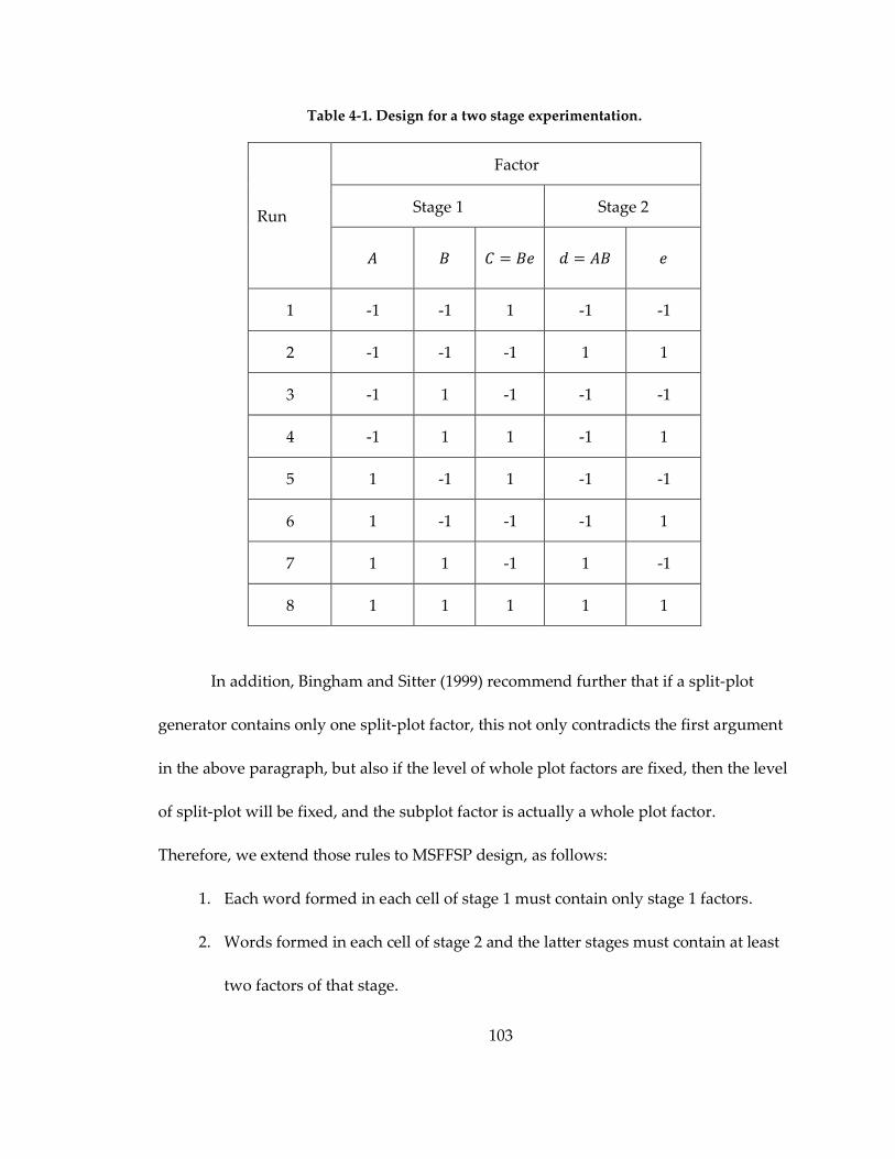
103
Table 4-1. Design for a two stage experimentation.
Run
Factor
Stage 1 Stage 2
𝐴 𝐵 𝐶 = 𝐵𝑒 𝑑 = 𝐴𝐵 𝑒
1 -1 -1 1 -1 -1
2 -1 -1 -1 1 1
3 -1 1 -1 -1 -1
4 -1 1 1 -1 1
5 1 -1 1 -1 -1
6 1 -1 -1 -1 1
7 1 1 -1 1 -1
8 1 1 1 1 1
In addition, Bingham and Sitter (1999) recommend further that if a split-plot
generator contains only one split-plot factor, this not only contradicts the first argument
in the above paragraph, but also if the level of whole plot factors are fixed, then the level
of split-plot will be fixed, and the subplot factor is actually a whole plot factor.
Therefore, we extend those rules to MSFFSP design, as follows:
1. Each word formed in each cell of stage 1 must contain only stage 1 factors.
2. Words formed in each cell of stage 2 and the latter stages must contain at least
two factors of that stage.
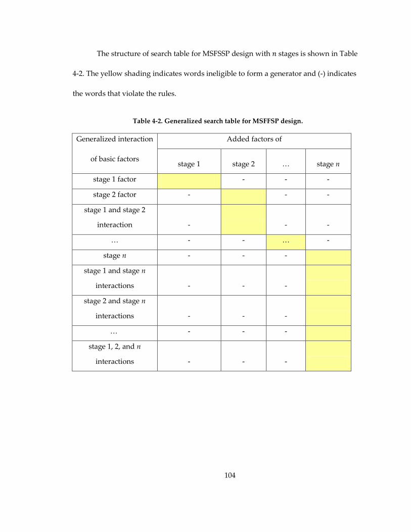
104
The structure of search table for MSFSSP design with 𝑛 stages is shown in Table
4-2. The yellow shading indicates words ineligible to form a generator and (-) indicates
the words that violate the rules.
Table 4-2. Generalized search table for MSFFSP design.
Generalized interaction
of basic factors
Added factors of
stage 1 stage 2 … stage n
stage 1 factor - - -
stage 2 factor - - -
stage 1 and stage 2
interaction - - -
… - - … -
stage n - - -
stage 1 and stage n
interactions - - -
stage 2 and stage n
interactions - - -
… - - -
stage 1, 2, and n
interactions - - -

105
Step 2: Construction of design generators
Once a search table for an experiment is constructed, generators are formed by
choosing a word from each column but not within the same row. If the words are chosen
from the same row, the design is of resolution II. The next step is to determine the
defining relation from those generators and the WLP for each generator. At this step, all
designs with maximum resolution are chosen, then, those designs are ranked based on
minimum aberration criteria. At the end of this step, several MA MSFFSP designs are
left and it is necessary to find the non-isomorphic designs.
Step 3: Find a non-isomorphic design
The simplest way to test for an isomorphic design is to construct the letter
pattern. The letter pattern is a matrix with size 𝑛 × 𝑛 where 𝑛 is the number of factors
and these factors are labeled as letters in the design. Elements 𝑎𝑖𝑗 of the letter pattern are
the number of letters 𝑖 appearing in the word length 𝑗 (𝑖, 𝑗 = 1, . . , n). However, designs
with the same letter pattern does not mean that they are isomorphic (Chen and Lin,
1991). Therefore, we have to continue testing with relabeling methods suggested by
Chen et al. (1993). The testing procedure is done by relabeling all factors. However,
when this method it is used in MSFFSP design, the factors will be only relabeled if they
are in the same stage due to a logical reason.
The algorithm presented here can be used for any MSFFSP designs with split-
plot structure, split block structure, and the combination of the two. However, their

106
analyses are different from their linear model.
4.4 An Example from the LMRIF Process
This section presents the development of an MA MSFFSP design on the factors of
the LMRIF process. The experiment involves seven factors with three stages as shown in
Table 4-3. If an FF design is used, 128 runs are required. However, based on
experimental budget constraints, only 32 runs are feasible. Therefore, we can only carry
out 1/8 of the total runs for this design.
Table 4-3. Factors of interest.
Factors of interest Levels
Stage 1: Particle
Preparation
(𝐴) Particle size 20 and 65 nm
(𝐵) Percent of volume loading 40 and 45 Vol%
(𝐶) Dispersant concentration 1.0 and 1.5 wt%
Stage 2: Gel
Casting
(𝑝) Percent of organic content 3.6 and 5 wt%
(𝑞) Initiator ratio (PEG:PVA) 1:1 and 1:1.5
Stage 3: Colloid
Deposition
(𝑈) Relative humidity 50 and 100%
(𝑉) Mold size (micro-scale) 25 and 100 microns
To create the search table in Table 4-4, we refer to the search table presented in
Table 4-2. The basic factors are 𝐴,𝐵,𝑃,𝑄, and 𝑈 and the added factors are 𝐶 and 𝑉. The
generalized interactions of basic factors followed by their stages are in the second

107
column and the basic factors are in the header of the third and fourth column. The
element represents the generalization of the column header and row header. The empty
lower left column (column 3) and the empty upper right column (column 4) follow the
rule (i), and rule (ii) in step 1, respectively.
Based on the search table in Table 4-4, there are 15 designs in total. The generator
of each design is formed the combination of a word from column 𝐶 and a word from
column 𝑉 , for example the generator for design number 1 is 𝐴𝐵𝐶,𝐴𝑈𝑉 with 𝑊𝐿𝑃 =
(0, 0, 2, 1, 0, 0, 0). However, there are only three designs of resolution III with minimum
aberration. Their 𝑊𝐿𝑃 are (0, 0, 1, 0, 1, 1, 0). The generators for those designs are: 𝐴𝐵𝐶,
𝐴𝑝𝑞𝑈𝑉; 𝐴𝐵𝐶,𝐵𝑝𝑞𝑈𝑉, and 𝐴𝐵𝐶,𝐴𝐵𝑝𝑞𝑈𝑉. All designs are isomorphic, therefore only the
following generator is selected: 𝐴𝐵𝐶,𝐴𝑝𝑞𝑈𝑉. Once the generator is chosen, the design
table for data collection is determined as shown in Table 4-5.
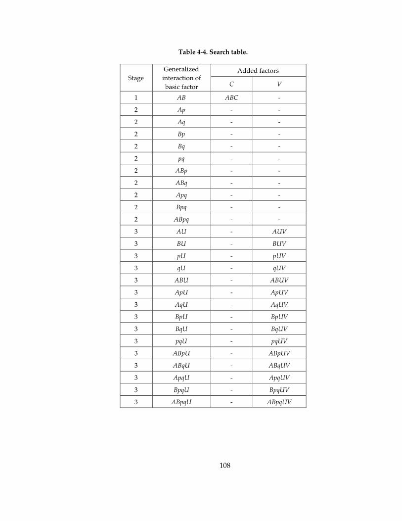
108
Table 4-4. Search table.
Stage
Generalized
interaction of
basic factor
Added factors
C V
1 AB ABC -
2 Ap - -
2 Aq - -
2 Bp - -
2 Bq - -
2 pq - -
2 ABp - -
2 ABq - -
2 Apq - -
2 Bpq - -
2 ABpq - -
3 AU - AUV
3 BU - BUV
3 pU - pUV
3 qU - qUV
3 ABU - ABUV
3 ApU - ApUV
3 AqU - AqUV
3 BpU - BpUV
3 BqU - BqUV
3 pqU - pqUV
3 ABpU - ABpUV
3 ABqU - ABqUV
3 ApqU - ApqUV
3 BpqU - BpqUV
3 ABpqU - ABpqUV
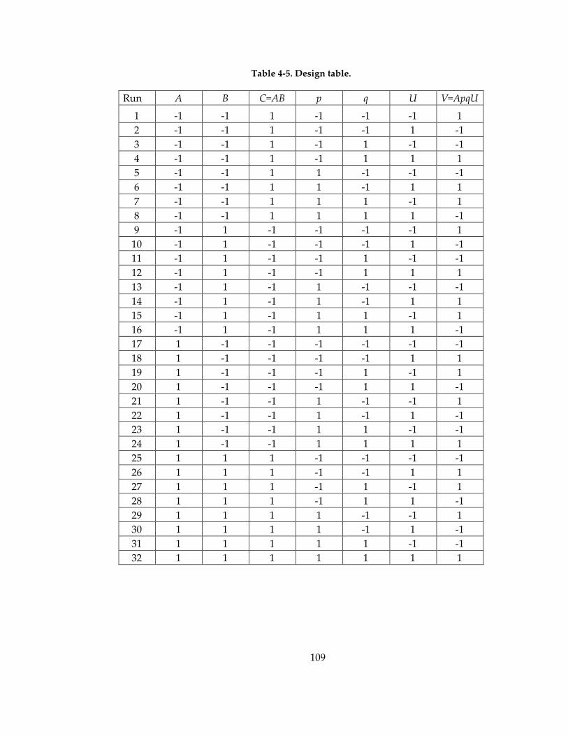
109
Table 4-5. Design table.
Run A B C=AB p q U V=ApqU
1 -1 -1 1 -1 -1 -1 1
2 -1 -1 1 -1 -1 1 -1
3 -1 -1 1 -1 1 -1 -1
4 -1 -1 1 -1 1 1 1
5 -1 -1 1 1 -1 -1 -1
6 -1 -1 1 1 -1 1 1
7 -1 -1 1 1 1 -1 1
8 -1 -1 1 1 1 1 -1
9 -1 1 -1 -1 -1 -1 1
10 -1 1 -1 -1 -1 1 -1
11 -1 1 -1 -1 1 -1 -1
12 -1 1 -1 -1 1 1 1
13 -1 1 -1 1 -1 -1 -1
14 -1 1 -1 1 -1 1 1
15 -1 1 -1 1 1 -1 1
16 -1 1 -1 1 1 1 -1
17 1 -1 -1 -1 -1 -1 -1
18 1 -1 -1 -1 -1 1 1
19 1 -1 -1 -1 1 -1 1
20 1 -1 -1 -1 1 1 -1
21 1 -1 -1 1 -1 -1 1
22 1 -1 -1 1 -1 1 -1
23 1 -1 -1 1 1 -1 -1
24 1 -1 -1 1 1 1 1
25 1 1 1 -1 -1 -1 -1
26 1 1 1 -1 -1 1 1
27 1 1 1 -1 1 -1 1
28 1 1 1 -1 1 1 -1
29 1 1 1 1 -1 -1 1
30 1 1 1 1 -1 1 -1
31 1 1 1 1 1 -1 -1
32 1 1 1 1 1 1 1

110
4.5 Design Catalogs
Using the new algorithm, we have created a design catalog for a three-stage
experiment by coding using MATLAB. Table 4-6 shows the design catalog for the three-
stage experiment. The number of factors in each stage is represented as 𝑛1 ,𝑛2 , and 𝑛3
and the number of fractionation in stage is 𝑘1 ,𝑘2, and 𝑘3 so the design can be
represented as 2(𝑛1−𝑘1) × 2(𝑛2−𝑘2) × 2(𝑛3−𝑘3). The number of runs and 𝑊𝐿𝑃 are also
given. Table 4-6 represents a design catalog for the four stage experiment.
Considering the LMRIF process, there are seven factors in total: three factors in
stage 1, two factors in stage 2 and two factors in stage 3. Since only 32 runs are required,
the design number 30 or 31, in Table 4-6, could be chosen. Narrowing the decision any
further could be based on the alias structure using additional process or scientific
knowledge. Based on discussion with the LMRIF scientists and engineers and taking
into account the information of interest, design number 30 is chosen and the design table
is shown in Table 4-6.
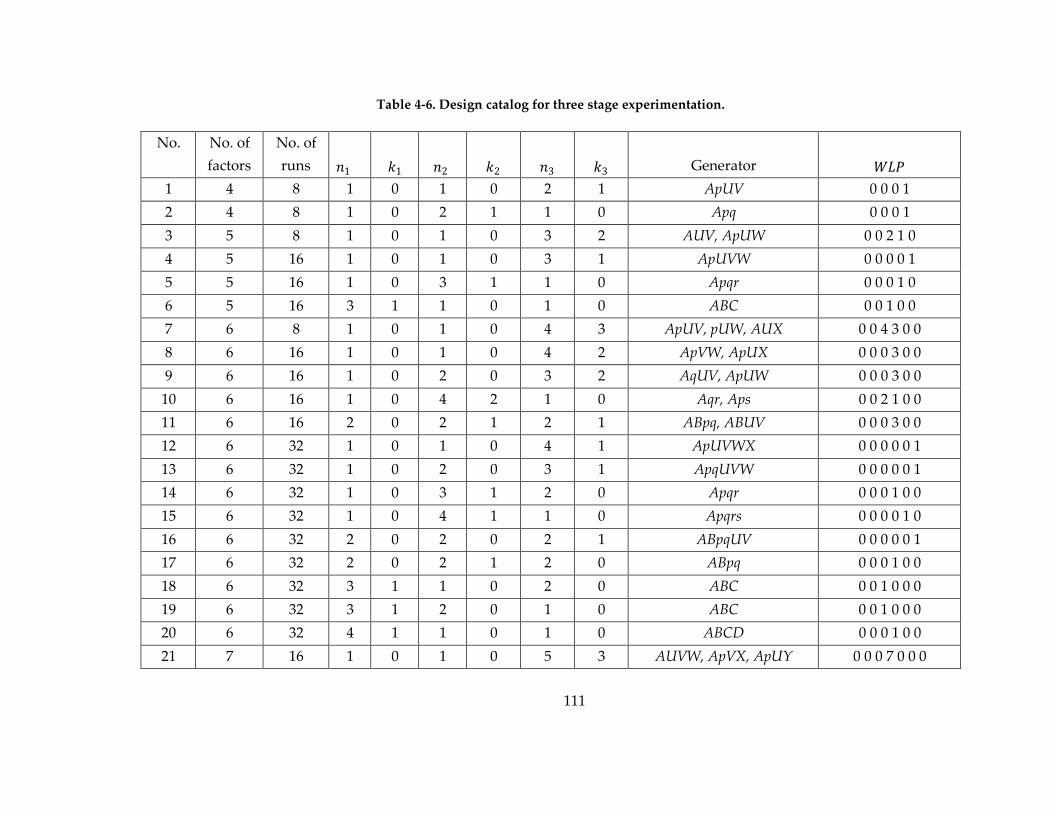
111
Table 4-6. Design catalog for three stage experimentation.
No. No. of
factors
No. of
runs 𝑛1 𝑘1 𝑛2 𝑘2 𝑛3 𝑘3 Generator 𝑊𝐿𝑃
1 4 8 1 0 1 0 2 1 ApUV 0 0 0 1
2 4 8 1 0 2 1 1 0 Apq 0 0 0 1
3 5 8 1 0 1 0 3 2 AUV, ApUW 0 0 2 1 0
4 5 16 1 0 1 0 3 1 ApUVW 0 0 0 0 1
5 5 16 1 0 3 1 1 0 Apqr 0 0 0 1 0
6 5 16 3 1 1 0 1 0 ABC 0 0 1 0 0
7 6 8 1 0 1 0 4 3 ApUV, pUW, AUX 0 0 4 3 0 0
8 6 16 1 0 1 0 4 2 ApVW, ApUX 0 0 0 3 0 0
9 6 16 1 0 2 0 3 2 AqUV, ApUW 0 0 0 3 0 0
10 6 16 1 0 4 2 1 0 Aqr, Aps 0 0 2 1 0 0
11 6 16 2 0 2 1 2 1 ABpq, ABUV 0 0 0 3 0 0
12 6 32 1 0 1 0 4 1 ApUVWX 0 0 0 0 0 1
13 6 32 1 0 2 0 3 1 ApqUVW 0 0 0 0 0 1
14 6 32 1 0 3 1 2 0 Apqr 0 0 0 1 0 0
15 6 32 1 0 4 1 1 0 Apqrs 0 0 0 0 1 0
16 6 32 2 0 2 0 2 1 ABpqUV 0 0 0 0 0 1
17 6 32 2 0 2 1 2 0 ABpq 0 0 0 1 0 0
18 6 32 3 1 1 0 2 0 ABC 0 0 1 0 0 0
19 6 32 3 1 2 0 1 0 ABC 0 0 1 0 0 0
20 6 32 4 1 1 0 1 0 ABCD 0 0 0 1 0 0
21 7 16 1 0 1 0 5 3 AUVW, ApVX, ApUY 0 0 0 7 0 0 0
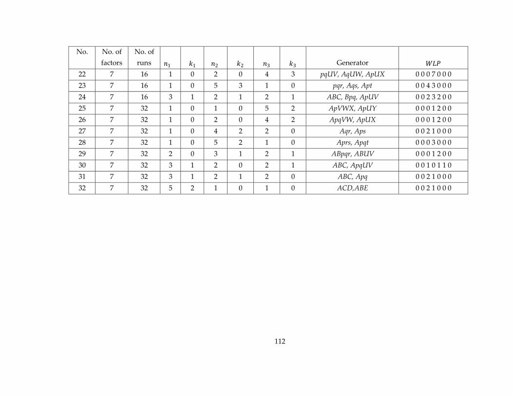
112
No. No. of
factors
No. of
runs 𝑛1 𝑘1 𝑛2 𝑘2 𝑛3 𝑘3 Generator 𝑊𝐿𝑃
22 7 16 1 0 2 0 4 3 pqUV, AqUW, ApUX 0 0 0 7 0 0 0
23 7 16 1 0 5 3 1 0 pqr, Aqs, Apt 0 0 4 3 0 0 0
24 7 16 3 1 2 1 2 1 ABC, Bpq, ApUV 0 0 2 3 2 0 0
25 7 32 1 0 1 0 5 2 ApVWX, ApUY 0 0 0 1 2 0 0
26 7 32 1 0 2 0 4 2 ApqVW, ApUX 0 0 0 1 2 0 0
27 7 32 1 0 4 2 2 0 Aqr, Aps 0 0 2 1 0 0 0
28 7 32 1 0 5 2 1 0 Aprs, Apqt 0 0 0 3 0 0 0
29 7 32 2 0 3 1 2 1 ABpqr, ABUV 0 0 0 1 2 0 0
30 7 32 3 1 2 0 2 1 ABC, ApqUV 0 0 1 0 1 1 0
31 7 32 3 1 2 1 2 0 ABC, Apq 0 0 2 1 0 0 0
32 7 32 5 2 1 0 1 0 ACD,ABE 0 0 2 1 0 0 0
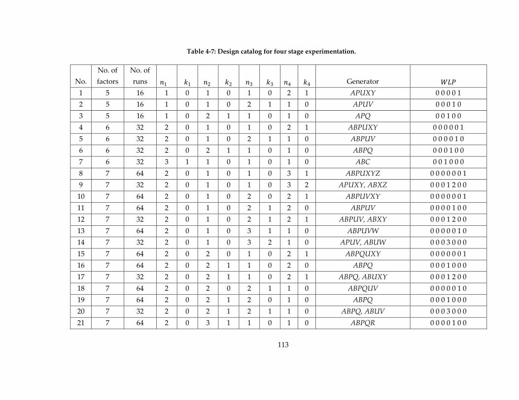
113
Table 4-7: Design catalog for four stage experimentation.
No.
No. of
factors
No. of
runs 𝑛1 𝑘1 𝑛2 𝑘2 𝑛3 𝑘3 𝑛4 𝑘4 Generator 𝑊𝐿𝑃
1 5 16 1 0 1 0 1 0 2 1 APUXY 0 0 0 0 1
2 5 16 1 0 1 0 2 1 1 0 APUV 0 0 0 1 0
3 5 16 1 0 2 1 1 0 1 0 APQ 0 0 1 0 0
4 6 32 2 0 1 0 1 0 2 1 ABPUXY 0 0 0 0 0 1
5 6 32 2 0 1 0 2 1 1 0 ABPUV 0 0 0 0 1 0
6 6 32 2 0 2 1 1 0 1 0 ABPQ 0 0 0 1 0 0
7 6 32 3 1 1 0 1 0 1 0 ABC 0 0 1 0 0 0
8 7 64 2 0 1 0 1 0 3 1 ABPUXYZ 0 0 0 0 0 0 1
9 7 32 2 0 1 0 1 0 3 2 APUXY, ABXZ 0 0 0 1 2 0 0
10 7 64 2 0 1 0 2 0 2 1 ABPUVXY 0 0 0 0 0 0 1
11 7 64 2 0 1 0 2 1 2 0 ABPUV 0 0 0 0 1 0 0
12 7 32 2 0 1 0 2 1 2 1 ABPUV, ABXY 0 0 0 1 2 0 0
13 7 64 2 0 1 0 3 1 1 0 ABPUVW 0 0 0 0 0 1 0
14 7 32 2 0 1 0 3 2 1 0 APUV, ABUW 0 0 0 3 0 0 0
15 7 64 2 0 2 0 1 0 2 1 ABPQUXY 0 0 0 0 0 0 1
16 7 64 2 0 2 1 1 0 2 0 ABPQ 0 0 0 1 0 0 0
17 7 32 2 0 2 1 1 0 2 1 ABPQ, ABUXY 0 0 0 1 2 0 0
18 7 64 2 0 2 0 2 1 1 0 ABPQUV 0 0 0 0 0 1 0
19 7 64 2 0 2 1 2 0 1 0 ABPQ 0 0 0 1 0 0 0
20 7 32 2 0 2 1 2 1 1 0 ABPQ, ABUV 0 0 0 3 0 0 0
21 7 64 2 0 3 1 1 0 1 0 ABPQR 0 0 0 0 1 0 0

114
No.
No. of
factors
No. of
runs 𝑛1 𝑘1 𝑛2 𝑘2 𝑛3 𝑘3 𝑛4 𝑘4 Generator 𝑊𝐿𝑃
22 7 32 2 0 3 2 1 0 1 0 BPQ, APR 0 0 2 1 0 0 0
23 7 32 2 0 3 2 1 0 1 0 ABPQ, APR 0 0 2 1 0 0 0
24 7 32 2 0 3 2 1 0 1 0 APQ, ABPR 0 0 2 1 0 0 0
25 7 64 3 0 1 0 1 0 2 1 ABCPUXY 0 0 0 0 0 0 1
26 7 64 3 1 1 0 1 0 2 0 ABC 0 0 1 0 0 0 0
27 7 32 3 1 1 0 1 0 2 1 ABC, APUXY 0 0 1 0 1 1 0
28 7 64 3 0 1 0 2 1 1 0 ABCPUV 0 0 0 0 0 1 0
29 7 64 3 1 1 0 2 0 1 0 ABC 0 0 1 0 0 0 0
30 7 32 3 1 1 0 2 1 1 0 ABC, APUV 0 0 1 1 1 0 0
31 7 64 3 0 2 1 1 0 1 0 ABCPQ 0 0 0 0 1 0 0
32 7 64 3 1 2 0 1 0 1 0 ABC 0 0 1 0 0 0 0
33 7 32 3 1 2 1 1 0 1 0 ABC, APQ 0 0 2 1 0 0 0

115
4.6 Remarks
The concepts presented in this chapter address the challenges of finding the
optimal designs based on maximum resolution and minimum aberration for multistage
experimentation. A new algorithm to search the MA MSFFSP design is developed. It
was applied to the LMRIF process, and design catalogs for three and four stage
experimentations were presented. The catalog can help experimenters to choose an
appropriate design to garner the maximum amount of important information from an
experiment. This will eventually speed up the cycle time of product and process
development.
In the next chapter, we discuss about how to apply the concept of robust
parameter design to MSFFSP design.

116
Chapter 5.
MSFFSP Designs for Robust Parameter Design
In this chapter, we present a multistage experiment associated with the concept
of robust parameter design (RPD) for the reduction of process and product variability.
We begin by introducing RPD in Section 5.1. Section 5.2 discusses the two main
characteristics of the LMRIF process that need special consideration when the RPD
concept is used. Section 5.3 presents the RPD modeling strategies. Section 5.4 discusses
how to use split-plot design with RPD, followed by design criteria for RPD MSFFSP
design in Section 5.5. Section 5.6 provides some design catalogs. An application of the
tool is shown in Section 5.7. Finally, the concluding remarks are presented in Section 5.8.
5.1 Introduction to Robust Parameter Design
One of the major concerns when scientists and engineers develop a new product
is the ability to reproduce a system, especially when they transfer it from the laboratory
scale to the manufacturing scale. The key to a smoother transfer is the reduction of the
variability in the system. There are several approaches to variability reduction: output
sampling inspection, statistical process monitoring and adjustment, variation reduction
in process inputs, covariate adjustment, and robust parameter design (RPD). Since our
research is applied to the development phase of making a forceps device, it is logical to
consider RPD and focus on how to make the process insensitive to input variation.

117
The concept of RPD was introduced by Taguchi and brought to the United States
in the mid 1980s6.This methodology has been widely used among engineers in practice
(Taguchi, 1987). RPD is a combination of statistical thinking and engineering
methodology. It is used to decrease the performance variation of a product or process by
properly setting controllable factors to make the process less sensitive to noise variation.
The factors of interest in RPD are divided into two types: controllable factors and
noise factors. Controllable factors are variables that are chosen at levels that are not
difficult to control. They can be the raw material types, process factors, and product
parameters. Noise factors are variables whose levels are uncontrolled or difficult to
control during the normal operation or at use conditions. They can be variation in raw
material, variation in product and process parameters, and environmental variation, and
variation in product-at-use condition. It is more effective and less costly to set levels of
controlled factors rather than to directly tighten noise factors.
RPD differs from other experimental designs in the sense that the interaction
among controllable factors and noise factors are as important as main effects. These
interactions indicate at which level controllable factors provide minimum variation. For
a complete review and discussion, see Nair (1992).
6 Box, in Nair (1992), pointed out that the concept of robust design was actually introduced by Michaels (1964)
and Morrison (1957), however this work did not get much attention.

118
5.2 LMRIF Process and RPD
To directly apply the RPD concept to the development of the lost mold rapid
infiltration forming (LMRIF) process is difficult because of its two main characteristics.
First, as mentioned in previous chapters, the process consists of several stages. This
prohibits experimenters from strictly following the randomization principle. Second,
there are multiple sets of noise factors as each stage is located in a different room.
For instance, Figure 5-1 shows three stages of an LMRIF process and an
additional stage when the forceps scissors (FS) are delivered to surgeons. It also shows
some controllable factors and noise factors in the (LMRIF) process. In the colloid
preparation, the controllable factors are solids loading percentage (% solid), gel
percentage (% gel), and binder percentage (% binder). The noise factors are chamber
temperature and humidity. For the colloid deposition, the filling direction and type of
chemical within the immersion bath can be controlled. Bath temperature and humidity
are considered noise factors. Note that sometimes some noise factors such as the
chamber temperature and bath temperature are controllable in laboratory settings;
however, when we move from the laboratory to manufacturing, they are not
controllable or are difficult to control. The objective of RPD for this process is to reduce
variation of percent yield (% yield).
In addition, by the time the FS is in a surgeon’s hand, there may be other factors
which are not controllable that affect the properties of the FS, such as conditions at use
and vibration during transportation. If we can determine the factors that affect the FS

119
properties, we can design the LMRIF process or packaging so that it will withstand
those variations.
Our investigation thus focuses on how to create an experimental design so that it
achieves robustness under the conditions of multiple stages and randomization
restriction of LMRIF process.
-% Solid-%Gel
-%Binder
Colloid Preparation
-Filling direction-Type of chemical
Colloid Deposition
Chamber temperureHumidity
Chemical temperatureHumidity
- Temperature profile
- Substrate location
Sintering
Ambient temperatureHumidity
Forceps scissors
Use conditionVibration during
transportation
Figure 5-1. Example of uncontrolled factors and noise factors in the LMRIF process.
5.3 RPD Modeling Strategies: Cross Array and Single Array
Let us consider an experiment at stage 1 of an LMRIF process where we have five
factors. The three controllable factors are % solid (A), % gel (B), and % binder (C) (as
shown the left block of Figure 5-1). The two noise factors are chamber temperature (d)
and humidity (e) are the noise factors (as shown the middle block of Figure 5-1). There
are only two levels (low level as -1 and high level as 1) for each factor. If we use the full
factorial design, then 32 runs and 32 settings for each factor are required. This design
will allow us to explore all main and interaction effects of the controllable factors and
noise factors. This serves the objective of RPD. However, suppose that only 16 runs are
allowed in this experiment. How can we choose a design generator for RPD purposes?

120
Wu and Hamada (2000) suggest that there are two strategies to be considered: cross
array and single array.
A cross array, introduced by Taguchi, involves two sets of experimental designs,
a control array and noise array, or they can be called the ‚inner array‛ and ‚outer array‛
respectively. The control array refers to a design matrix dealing with controllable factors,
while noise factors involve the noise array. Mathematically, the total number of runs is
the product of the number of runs of the control array and noise array. If the cross array
is used for controllable factors, it means noise factors should be systematically varied
because they are difficult to control in normal conditions. This type of design allows us
to estimate the interaction between controllable factors and noise factors that is not
confounded with main effects or other interactions. These types of interactions are very
important for RPD. From this point onward, we will use the letter 𝑪 to represent a
controllable factor and 𝑵 to represent a noise factor. The notation 𝑪 × 𝑪, 𝑪 × 𝑵, 𝑵 × 𝑵
represent interaction between 𝑪 and 𝑪 , 𝑪 and 𝑵, and 𝑵 and 𝑵, respectively.
However, this design requires a large number of runs. To reduce the number of
runs in the cross array design, the fractionation can be done only ‚within-stage‛
confounding. The results in the 𝑪 × 𝑪 interaction are aliased with 𝑪 main effects, and the
results in the 𝑵 × 𝑵 interaction are aliased with 𝑵 main effects. In the LMRIF case, the
only generator we can choose is 𝐼 = 𝐴𝐵𝐶 (to maintain the split-plot structure). Table 5-1
illustrates the experimental design for the process in Figure 5-1.
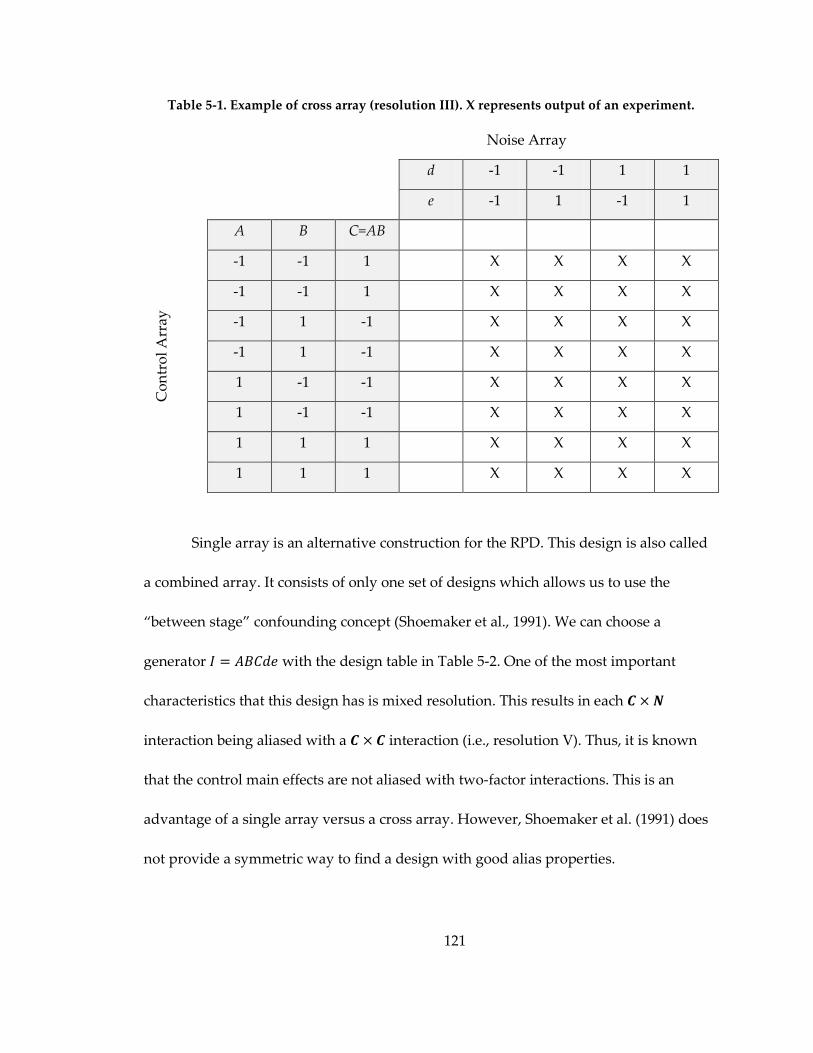
121
Table 5-1. Example of cross array (resolution III). X represents output of an experiment.
Noise Array
d -1 -1 1 1
e -1 1 -1 1
Co
ntr
ol
Arr
ay
A B C=AB
-1 -1 1 X X X X
-1 -1 1 X X X X
-1 1 -1 X X X X
-1 1 -1 X X X X
1 -1 -1 X X X X
1 -1 -1 X X X X
1 1 1 X X X X
1 1 1 X X X X
Single array is an alternative construction for the RPD. This design is also called
a combined array. It consists of only one set of designs which allows us to use the
‚between stage‛ confounding concept (Shoemaker et al., 1991). We can choose a
generator 𝐼 = 𝐴𝐵𝐶𝑑𝑒 with the design table in Table 5-2. One of the most important
characteristics that this design has is mixed resolution. This results in each 𝑪 × 𝑵
interaction being aliased with a 𝑪 × 𝑪 interaction (i.e., resolution V). Thus, it is known
that the control main effects are not aliased with two-factor interactions. This is an
advantage of a single array versus a cross array. However, Shoemaker et al. (1991) does
not provide a symmetric way to find a design with good alias properties.
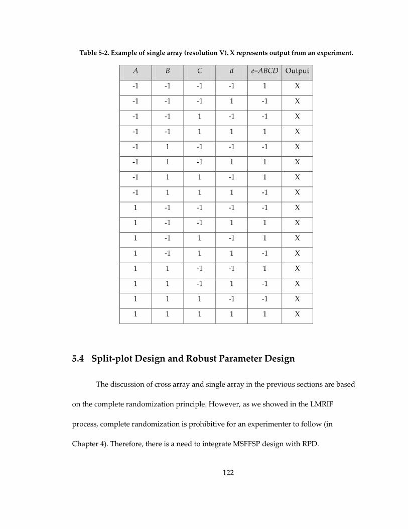
122
Table 5-2. Example of single array (resolution V). X represents output from an experiment.
A B C d e=ABCD Output
-1 -1 -1 -1 1 X
-1 -1 -1 1 -1 X
-1 -1 1 -1 -1 X
-1 -1 1 1 1 X
-1 1 -1 -1 -1 X
-1 1 -1 1 1 X
-1 1 1 -1 1 X
-1 1 1 1 -1 X
1 -1 -1 -1 -1 X
1 -1 -1 1 1 X
1 -1 1 -1 1 X
1 -1 1 1 -1 X
1 1 -1 -1 1 X
1 1 -1 1 -1 X
1 1 1 -1 -1 X
1 1 1 1 1 X
5.4 Split-plot Design and Robust Parameter Design
The discussion of cross array and single array in the previous sections are based
on the complete randomization principle. However, as we showed in the LMRIF
process, complete randomization is prohibitive for an experimenter to follow (in
Chapter 4). Therefore, there is a need to integrate MSFFSP design with RPD.

123
The pioneering study of using split-plot design with RPD was proposed by Box
and Jones (1992). They demonstrated how to use a split-plot to design a cake-mix
experiment so that a product is insensitive to environmental factors (noise factors). They
propose three different arrangements:
1. Control factors as whole-plot factors and noise factors as sub-plot factors
2. Control factors as sub-plot factors and noise factors as whole-plot factors
3. Control factors and noise factors arranged in the split block structure
These three arrangements can be chosen based on the experimenters’ convenience
The fractionation of the split-plot design for robust study is found in Bisgaard and
Steinberg (1997); however, they do not consider the fractionation of both control and
noise design arrays. They propose a design and analysis for an experimentation with
control factors as whole plot factor under fractional factorial designs while noise factors
are arranged in full factorial design. Later, Bisgaard (2000) suggested using ‚inner
array‛ and ‚outer array‛ as ‚whole-plot‛ and/or ‚sub-plot‛ arrangements for a large
Taguchi experiment.
Bingham and Sitter (2003) provided a complete study of how to use fractional
factorial design with split-plot arrangement. The control factors and noise factors are
considered whole plot or split-plot type of factors. Catalog design with 16 runs and 32
runs are also provided. We will discuss in more detail the criteria they use in their study
in the next section.

124
5.5 Design Criteria for RPD MSFFSP Design
5.5.1 Effect Ordering Principle for RPD
It is important in RPD to consider the interactions of the 𝑪 and 𝑵 factors. This is
because we need to find a proper setting of 𝑪 so that the output response variation is
minimized. Therefore, the importance of the factors are ranked as 𝑪,𝑪𝑵,𝑪𝑪,𝑪𝑪𝑵.
Wu and Zhu (2003) proposed a numerical rule to rank all effects based on their
weight (𝑊(𝑖, 𝑗)) where 𝑖 𝑖 = 1. .𝑘 , 𝑖 ∶the number of 𝑪 appearing in the effect and
𝑗(𝑗 = 1. .𝑘), 𝑗: is the number of 𝑵 appearing in the effect, and 𝑖 + 𝑗 = 𝑘 is the number of
total factors. These rules are defined in the following equation:
𝑊 𝑖, 𝑗 = 1 𝑖
𝑗 + 1/2
𝑖𝑓 𝑖𝑓𝑖𝑓
max 𝑖, 𝑗 = 1𝑖 > 𝑗 𝑎𝑛𝑑 𝑖 ≥ 1𝑖 ≤ 𝑗 𝑎𝑛𝑑 𝑗 ≥ 2
(5-1)
Therefore 𝑊 = 1, 2, 2.5, 3,…. Let 𝐾𝑤 be the set of effects with weight 𝑊. Then
𝐾1 = 𝑪,𝑵,𝑪𝑵 , 𝐾2 = 𝑪𝑪,𝑪𝑪𝑵 , 𝐾2.5 = 𝑪𝑪𝑵𝑵,𝑪𝑵𝑵,𝑵𝑵 , and so on. These 𝐾 sets are
similar to the modified word length pattern ranking given by Bingham and Sitter (2003).
From these sets, we can observe that effects with smaller weight are more important
than those with larger weight. Effects with similar weight are equally important. This
leads to ranking as shown in Table 5-1. Note that Wu and Zhu (2003) only considered
the case of complete randomization while Bingham and Sitter (2003) also considered the
case of restriction on randomization.

125
Table 5-1. Ranking for RPD suggested by Wu and Zhu (2003).
Ranking (𝐾𝑊) Word
1.0 𝑪,𝑵,𝑪𝑵
2.0 𝑪𝑪,𝑪𝑪𝑵
2.5 𝑪𝑪𝑵𝑵,𝑪𝑵𝑵,𝑵𝑵
3.0 𝑪𝑪𝑪,𝑪𝑪𝑪𝑵,𝑪𝑪𝑪𝑵𝑵
4.0 𝑵𝑵𝑵,𝑪𝑪𝑪𝑪,𝑪𝑪𝑪𝑪𝑵,𝑪𝑪𝑪𝑪𝑵𝑵,𝑪𝑪𝑪𝑪𝑵𝑵𝑵
Another ranking was introduced by Bingham and Sitter (2003). They used an
effect-ordering principle slightly different to those in Wu and Zhu (2003). They
proposed the concept of likely significance and effect importance to experimenters as
shown in Table 5-2 . Then the ranking of effects for the interaction of three factors can be
grouped as in Table 5-2.
Table 5-2. Effect ranking for robust parameter design (Bingham and Sitter, 2003).
Ranking Likely significance Interest (for RPD)
1 𝑪,𝑵 𝑪,𝑪𝑵
2 𝑪𝑪,𝑪𝑵,𝑵𝑵 𝑪𝑪,𝑪𝑪𝑵,𝑪𝑵𝑵
3 𝑪𝑪𝑪,𝑪𝑪𝑵,𝑪𝑵𝑵,𝑵𝑵𝑵 𝑪𝑪𝑪

126
Table 5-3. Ranking for RPD suggested by Bingham and Sitter (2003).
Ranking (WLP) Word
1.0 𝑪,𝑵
1.5 𝑪𝑵
2.0 𝑪𝑪,𝑵𝑵
2.5 𝑪𝑪𝑵,𝑪𝑵𝑵
3.0 𝑪𝑪𝑪
4.0 𝑵𝑵𝑵
The resolution and MA are defined as the minimum number of words of each
length as they related to the forgoing word hierarchy. For example, in resolution IV,
there is a word with a length of four letters in the defining relation. That word consists
of one word of length one and one word of length three or two words of length two.
Therefore the resolution is the minimum of the sum of lengths of the two words (i.e., 1+3
= 4 and 2+2=4). Bingham and Sitter (2003) used this concept but modified the world
length definition to obtain the new word length as shown in Table 5-3.

127
Table 5-4. Word lengths pattern for RPD MSFFSP design.
WLP Word
1.0 𝑪,𝑵
1.5 𝑪𝑵
2.0 𝑪𝑪,𝑵𝑵
2.5 𝑪𝑪𝑵,𝑪𝑵𝑵
3.0 𝑪𝑪𝑪,𝑪𝑪𝑵𝑵
3.5 𝑪𝑪𝑪𝑵,𝑪𝑵𝑵𝑵
4.0 𝑪𝑪𝑪𝑪,𝑵𝑵𝑵,𝑪𝑪𝑪𝑵𝑵,𝑪𝑪𝑵𝑵𝑵
4.5 𝑪𝑪𝑪𝑪𝑵,𝑪𝑵𝑵𝑵𝑵
5.0 𝑪𝑪𝑪𝑪𝑪,𝑵𝑵𝑵𝑵,𝑪𝑪𝑪𝑵𝑵𝑵,𝑪𝑪𝑵𝑵𝑵𝑵,𝑪𝑪𝑪𝑪𝑵𝑵
5.5 𝑪𝑪𝑪𝑪𝑪𝑵,𝑪𝑵𝑵𝑵𝑵𝑵
6.0 𝑪𝑪𝑪𝑪𝑪𝑪,𝑵𝑵𝑵𝑵𝑵,𝑪𝑪𝑪𝑪𝑪𝑵𝑵,𝑪𝑪𝑪𝑪𝑵𝑵𝑵,𝑪𝑪𝑪𝑵𝑵𝑵𝑵,𝑪𝑪𝑵𝑵𝑵𝑵𝑵
6.5 𝑪𝑪𝑪𝑪𝑪𝑪𝑵,𝑪𝑵𝑵𝑵𝑵𝑵𝑵
… …
As illustrated, both principles lie in the same direction but they are different in
the sense of accounting for the effects of controllable factors and their interactions with
noise factors. In this research, we extend the idea of the effect-ordering principle
suggested by Bingham and Sitter (2003). This is because the principle is based on likely
significance and effects importance and it provides a balance between effect estimation
with the aliasing of lower-order terms. Bingham and Sitter (2003)’s use of the minimum
aberration criteria provides a clearer roadmap for extensions than those of Zhu and Wu
(2003)’s where their focus is only on the effects importance. In addition, since the LMRIF
process is under development, the main effects (𝑊𝐿𝑃 = 1) are more important than the

128
interaction of control factors and noise factors (𝑊𝐿𝑃 = 1.5). It is also the case that the
interaction of control and noise factors (𝑊𝐿𝑃 = 1.5) is more important than the
interaction of control factors (𝑊𝐿𝑃 = 2.0). The noise factors may become control factors
if they are significant and affect the process performance. Therefore, Bingham and Sitter
(2003)’s raking approach where 𝑊𝐿𝑃 = 1.5 for the interaction of control and noise
factors is more suitable to the LMRIF process experimentation.
5.5.2 MSFFSP Design with RPD
In the last section, we describe the concept of using modified resolution as a
criterion to rank designs in a robust study. Like MSFFSP design, MSFFSP designs with
RPD (RPD MSFFSP) designs are not all equally good. A major feature of RPD MSFFSP
designs that distinguishes them from RPD MSFFSP design is that in MSFFSP design, we
consider only controllable factors whereas in RPD MSFFSP design, there are both
controllable factors and noise factors in each stage. Secondly, both types of factors can be
either whole plot or sub plot factors. To deal with these differences, we need to modify
our experimental structure by splitting up the factors of each stage into two groups (𝑪
and N) and separating them into different stages.
For example, consider the process in Figure 5-1 without noise factors in colloid
deposition. After splitting the factors into stages, there are three sets of C factors and N
factors. There is one set of C factors and one set N factors in stage 1, and one set of C
factors in stage 2. Suppose that we set C factors in stage 1 as a whole plot and N factors in

129
stage 1 as a subplot followed by C factors in stage 2. The structure can be represented by
CNC. Once the structure of the experimentation is determined, it is similar to the design
catalog for the MSFFSP design as shown in Chapter 4 with the modified resolution.
5.5.3 Finding the Optimal RPD MSFFSP Design
Once the structure of the experimentation has been determined, we can then
apply the algorithm presented in Section 4.3 directly, except that the modified WLP is
used instead of the regular WLP. The MATLAB is used to code this procedure.
5.6 Some Design Catalogs
There are several design structures that can be represented with the RPD
MSFFSP experiments. We construct design catalogs where there are two stages with
three sets of factors and only one set of noise factors. There are three cases:
Case 1: In stage 1, there is one set of controlled factors and in stage 2 there are
both types of factors (𝑪𝑪𝑵).
Case 2: In stage 1, there are two sets of factor. The controllable factor is a whole
plot and noise factors are a subplot, and there is one controllable factor in stage 2 (𝑪𝑵𝑪).
Case 3: In stage 1 there are two sets of factors, the noise factor is a whole plot and
controllable factors are a subplot, and there is one set of controllable factors in stage 2
(𝑵𝑪𝑪).
Tables 5-5, 5-6, and 5-7 are design catalogs for case 1, case 2 and case 3,

130
respectively. The number of factors in each stage can be represented as 𝑛1 ,𝑛2 , and 𝑛3
where 𝑘1 ,𝑘2 , and 𝑘3 are the number of fractionations in stages 1, 2, and 3, respectively.
The design can be represented as 2𝑛1−𝑘1 × 2𝑛2−𝑘2 × 2𝑛3−𝑘3 . The number of runs and the
WLP are also given in the tables.
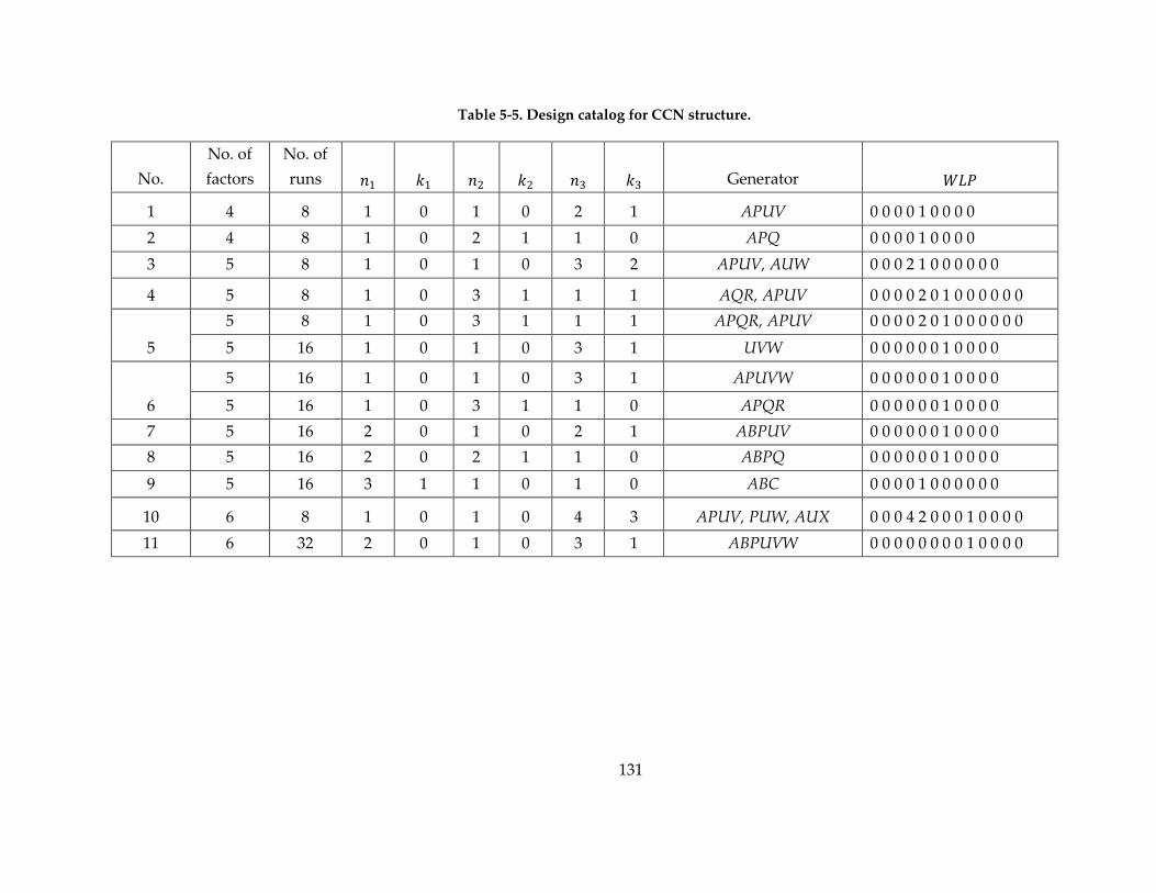
131
Table 5-5. Design catalog for CCN structure.
No.
No. of
factors
No. of
runs 𝑛1 𝑘1 𝑛2 𝑘2 𝑛3 𝑘3 Generator 𝑊𝐿𝑃
1 4 8 1 0 1 0 2 1 APUV 0 0 0 0 1 0 0 0 0
2 4 8 1 0 2 1 1 0 APQ 0 0 0 0 1 0 0 0 0
3 5 8 1 0 1 0 3 2 APUV, AUW 0 0 0 2 1 0 0 0 0 0 0
4 5 8 1 0 3 1 1 1 AQR, APUV 0 0 0 0 2 0 1 0 0 0 0 0 0
5
5 8 1 0 3 1 1 1 APQR, APUV 0 0 0 0 2 0 1 0 0 0 0 0 0
5 16 1 0 1 0 3 1 UVW 0 0 0 0 0 0 1 0 0 0 0
6
5 16 1 0 1 0 3 1 APUVW 0 0 0 0 0 0 1 0 0 0 0
5 16 1 0 3 1 1 0 APQR 0 0 0 0 0 0 1 0 0 0 0
7 5 16 2 0 1 0 2 1 ABPUV 0 0 0 0 0 0 1 0 0 0 0
8 5 16 2 0 2 1 1 0 ABPQ 0 0 0 0 0 0 1 0 0 0 0
9 5 16 3 1 1 0 1 0 ABC 0 0 0 0 1 0 0 0 0 0 0
10 6 8 1 0 1 0 4 3 APUV, PUW, AUX 0 0 0 4 2 0 0 0 1 0 0 0 0
11 6 32 2 0 1 0 3 1 ABPUVW 0 0 0 0 0 0 0 0 1 0 0 0 0
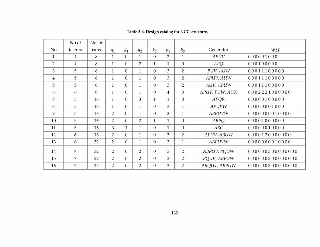
132
Table 5-6. Design catalog for NCC structure.
No
No of
factors
No. of
runs 𝑛1 𝑘1 𝑛2 𝑘2 𝑛3 𝑘3 Generator 𝑊𝐿𝑃
1 4 8 1 0 1 0 2 1 APUV 0 0 0 0 0 1 0 0 0
2 4 8 1 0 2 1 1 0 APQ 0 0 0 1 0 0 0 0 0
3 5 8 1 0 1 0 3 2 PUV, AUW 0 0 0 1 1 1 0 0 0 0 0
4 5 8 1 0 1 0 3 2 APUV, AUW 0 0 0 1 1 1 0 0 0 0 0
5 5 8 1 0 1 0 3 2 AUV, APUW 0 0 0 1 1 1 0 0 0 0 0
6 6 8 1 0 1 0 4 3 APUV, PUW, AUX 0 0 0 2 2 2 1 0 0 0 0 0 0
7 5 16 1 0 3 1 1 0 APQR 0 0 0 0 0 1 0 0 0 0 0
8 5 16 1 0 1 0 3 1 APUVW 0 0 0 0 0 0 0 1 0 0 0
9 5 16 2 0 1 0 2 1 ABPUVW 0 0 0 0 0 0 0 0 1 0 0 0 0
10 5 16 2 0 2 1 1 0 ABPQ 0 0 0 0 1 0 0 0 0 0 0
11 5 16 3 1 1 0 1 0 ABC 0 0 0 0 0 0 1 0 0 0 0
12 6 16 2 0 1 0 3 2 APUV, ABUW 0 0 0 0 1 2 0 0 0 0 0 0 0
13 6 32 2 0 1 0 3 1 ABPUVW 0 0 0 0 0 0 0 0 1 0 0 0 0
14 7 32 2 0 2 0 3 2 ABPUV, PQUW 0 0 0 0 0 0 3 0 0 0 0 0 0 0 0
15 7 32 2 0 2 0 3 2 PQUV, ABPUW 0 0 0 0 0 0 3 0 0 0 0 0 0 0 0
16 7 32 2 0 2 0 3 2 ABQUV, ABPUW 0 0 0 0 0 0 3 0 0 0 0 0 0 0 0
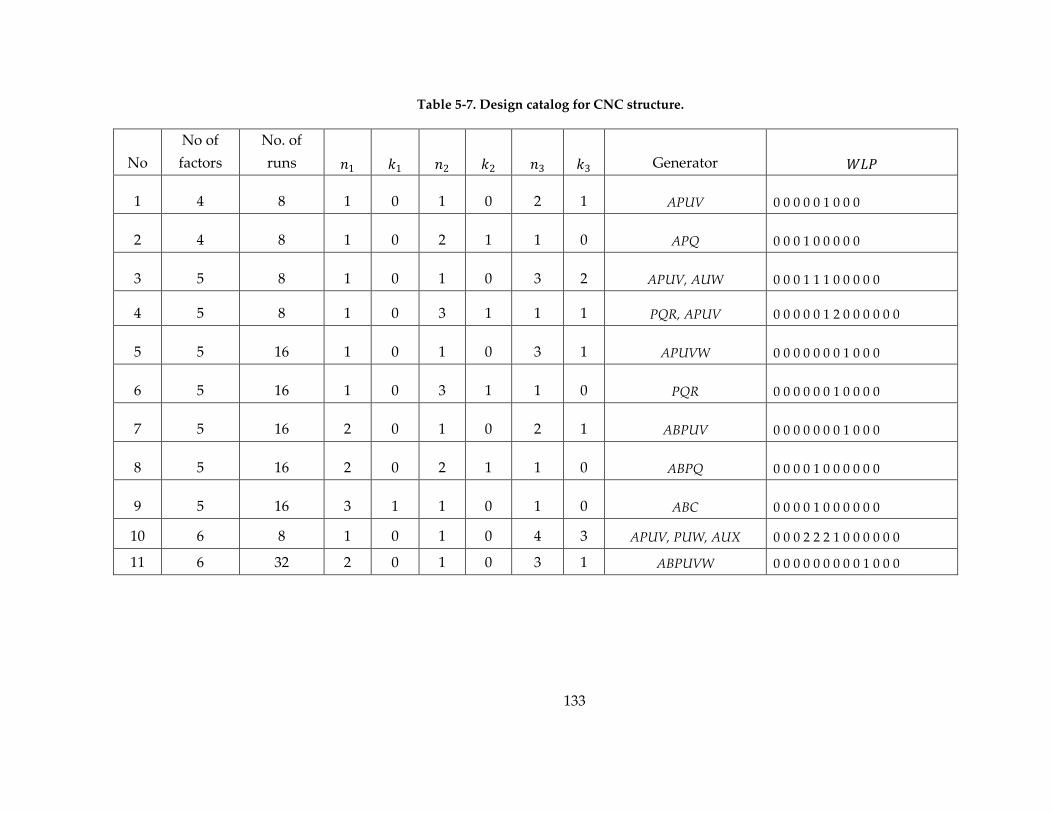
133
Table 5-7. Design catalog for CNC structure.
No
No of
factors
No. of
runs 𝑛1 𝑘1 𝑛2 𝑘2 𝑛3 𝑘3 Generator 𝑊𝐿𝑃
1 4 8 1 0 1 0 2 1 APUV 0 0 0 0 0 1 0 0 0
2 4 8 1 0 2 1 1 0 APQ 0 0 0 1 0 0 0 0 0
3 5 8 1 0 1 0 3 2 APUV, AUW 0 0 0 1 1 1 0 0 0 0 0
4 5 8 1 0 3 1 1 1 PQR, APUV 0 0 0 0 0 1 2 0 0 0 0 0 0
5 5 16 1 0 1 0 3 1 APUVW 0 0 0 0 0 0 0 1 0 0 0
6 5 16 1 0 3 1 1 0 PQR 0 0 0 0 0 0 1 0 0 0 0
7 5 16 2 0 1 0 2 1 ABPUV 0 0 0 0 0 0 0 1 0 0 0
8 5 16 2 0 2 1 1 0 ABPQ 0 0 0 0 1 0 0 0 0 0 0
9 5 16 3 1 1 0 1 0 ABC 0 0 0 0 1 0 0 0 0 0 0
10 6 8 1 0 1 0 4 3 APUV, PUW, AUX 0 0 0 2 2 2 1 0 0 0 0 0 0
11 6 32 2 0 1 0 3 1 ABPUVW 0 0 0 0 0 0 0 0 0 1 0 0 0
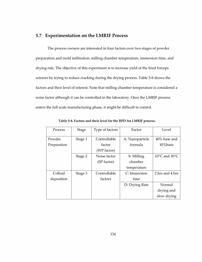
134
5.7 Experimentation on the LMRIF Process
The process owners are interested in four factors over two stages of powder
preparation and mold infiltration: milling chamber temperature, immersion time, and
drying rate. The objective of this experiment is to increase yield of the fired forceps
scissors by trying to reduce cracking during the drying process. Table 5-8 shows the
factors and their level of interest. Note that milling chamber temperature is considered a
noise factor although it can be controlled in the laboratory. Once the LMRIF process
enters the full scale manufacturing phase, it might be difficult to control.
Table 5-8. Factors and their level for the RPD for LMRIF process.
Process Stage Type of factors Factor Level
Powder
Preparation
Stage 1 Controllable
factor
(WP factor)
A: Nanoparticle
formula
40% base and
45%base
Stage 2 Noise factor
(SP factor)
b: Milling
chamber
temperature
10°C and 30°C
Colloid
deposition
Stage 3 Controllable
factors
C: Immersion
time
2 hrs and 4 hrs
D: Drying Rate Normal
drying and
slow drying
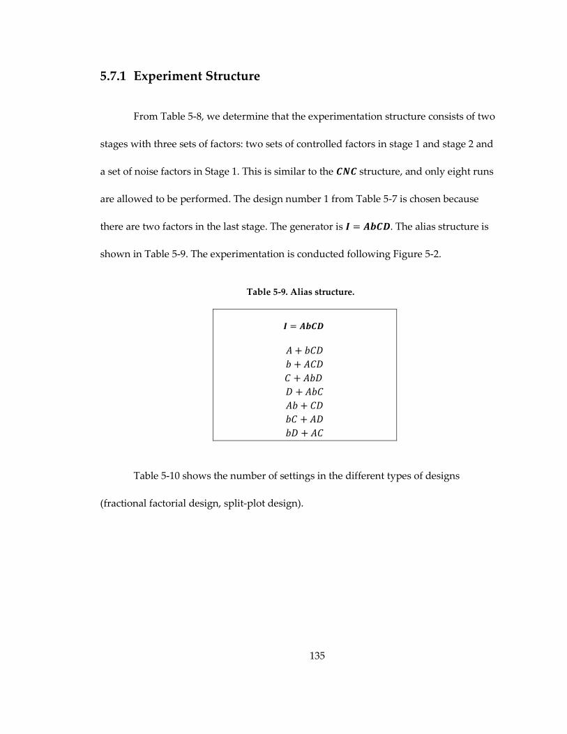
135
5.7.1 Experiment Structure
From Table 5-8, we determine that the experimentation structure consists of two
stages with three sets of factors: two sets of controlled factors in stage 1 and stage 2 and
a set of noise factors in Stage 1. This is similar to the 𝑪𝑵𝑪 structure, and only eight runs
are allowed to be performed. The design number 1 from Table 5-7 is chosen because
there are two factors in the last stage. The generator is 𝑰 = 𝑨𝒃𝑪𝑫. The alias structure is
shown in Table 5-9. The experimentation is conducted following Figure 5-2.
Table 5-9. Alias structure.
𝑰 = 𝑨𝒃𝑪𝑫
𝐴 + 𝑏𝐶𝐷
𝑏 + 𝐴𝐶𝐷
𝐶 + 𝐴𝑏𝐷
𝐷 + 𝐴𝑏𝐶
𝐴𝑏 + 𝐶𝐷
𝑏𝐶 + 𝐴𝐷
𝑏𝐷 + 𝐴𝐶
Table 5-10 shows the number of settings in the different types of designs
(fractional factorial design, split-plot design).

136
Table 5-10. Number of settings in the RPD MSFFSP design.
Design Number of settings in Number
of runs Stage 1 Stage 2 Stage 3
FF(24−1) 8 8 8 8
MSFFSP
(23−1 × 21 × 21)
Split-Plot 2 4 8 8
Split-Block 2 2 2 8
11
12
111
1
111 114
21
222
21
22
2
12
Stage 1
(2 settings)
Stage 2
(4 settings)
Stage 3
(8 settings)
122
123
212
213
221
224
Figure 5-2. Experimentation for RPD

137
Figure 5-2 describes the experimental work. In stage 1, two pre-mixed
nanoparticle suspensions are prepared with two treatment conditions (yellow-shaded)
of formula (𝐴). Then, in stage 2, each unit is split into two groups for two treatments
(green-shaded) of milling temperature(𝑏). Then, in stage 3, each group is split and then
they are applied to a treatment combination of immersion time (𝐶) in the ethanol and
drying type (𝐷) (blue-shaded). The number labeled in each block refers to the
experiment unit number, for example label 122 indicates that this experimental unit is
performed with treatment combination no. 1 from stage 1, with treatment combination
no. 2 from stage 2, with treatment combination no. 2 from stage 3).
5.7.1.1 Linear Model
Since this experiment uses only split-plot structure, its linear model is given by
Equation 3-4. Assuming that there are 𝑎 levels of a stage 1 factor, 𝑏 levels of a stage 2
factor, 𝑐 levels of stage 3, and 𝑛 replicates, the linear model for this design structure is
𝑦𝑔𝑖𝑗 = 𝜇 + 𝜌𝑔 + 𝛼 + 𝜖𝑔𝑠1 + 𝛽𝑖 + 𝛼𝛽𝑖 + 𝜖𝑔𝑖
𝑠2 + 𝛾𝑗+𝛼𝛾𝑗 + +𝛽𝛾𝑖𝑗
+𝛼𝛽𝛾𝑖𝑗 + 𝜖𝑔𝑖𝑗 𝑠3
(5-1)
where
𝑦𝑔𝑖 is the 𝑔𝑖𝑗𝑡 response of the experiment,
𝜇 is a general overall mean effect,
𝜌𝑔 is the 𝑔𝑡 replicate effect 𝑁 0,𝜎𝜌2 ~𝑖𝑖𝑑,
𝛼 is the effect of gth level of stage 1 factor,

138
𝜖𝑔𝑠1 is the 𝑔𝑡 random error effect 𝑁 0,𝜎𝜖𝑠1
2 ~𝑖𝑖𝑑,
𝛽𝑖 is the effect of 𝑖𝑡 level of stage 2 factors,
𝛼𝛽 is the interaction effect of 𝑖𝑡 combination of stage 1 and 2 factor,
𝜖𝑔𝑖𝑠2 is the 𝑔𝑖𝑡 random error effect 𝑁 0,𝜎𝜖𝑠1
2 ~𝑖𝑖𝑑,
𝛾𝑗 is the effect of 𝑗𝑡 level of stage 3 factor,
𝛼𝛾𝑗 is the interaction effect of 𝑗𝑡 combination of stage 1, and 3 factor,
𝛽𝛾𝑖𝑗 is the interaction effect of 𝑖𝑗𝑡 combination of stage 2, and 3 factor,
𝛼𝛽𝛾𝑖𝑗 is the interaction effect of 𝑖𝑗𝑡 combination of stage 1, 2, and 3 factor,
𝜖𝑔𝑖𝑗𝑠3 is the 𝑔𝑗𝑡 random error effect 𝑁 0,𝜎𝜖𝑠3
2 ~𝑖𝑖𝑑.
All errors are mutually independent.
Note that the superscript of each error term indicates the stage number and its
interaction with factors from other stages, for example, 𝜖𝑔𝑖𝑗𝑠3 is the error term due to the
interaction among factors from stage 3.
From the linear model in Equation (5-1), there are three error terms, which
indicates that there are three error terms in total, the first three error terms correspond to
effects of the first three stage factors, respectively. The other three error terms
correspond to interaction effects among stage 1 and stage 2, stage 2 and stage 3 and
stage 1, stage 2 and stage 3. It is important to know which contrasts will be tested
against which error term in order to test for significance. For this experiment, Table 5-11
summarizes the contrast effects and their error structure.

139
Table 5-11. Contrast effects and their error structure in the MSSP design. Only main and
second-order terms are displayed.
Contrast Error term
𝐴 𝜖𝑔𝑠1
𝑏,𝐴𝑏 𝜖𝑔𝑖
𝑠2
𝐶,𝐷, 𝑏𝐶, 𝑏𝐷
𝜖𝑔𝑗𝑠3
5.7.2 Results and Discussion
In this experiment, the yield of fired forceps is considered. Intact forceps are
counted then divided by the total number of forceps fabricated. The results of the
experiment, in Table 5-12, are analyzed using the general linear model capability in the
Minitab software. All mean square errors have been calculated with selected effects
regrouped and reorganized with the associated error terms based on Table 5-13.
Table 5-12. Experimentation runs and results.
A b C D=AbC
Yield
Rep1 Rep2
-1 -1 -1 -1 37.50 33.33
-1 -1 1 1 45.83 16.67
-1 1 -1 1 79.17 20.83
-1 1 1 -1 54.17 20.83
1 -1 -1 1 37.50 25.00
1 -1 1 -1 29.17 0.00
1 1 -1 -1 29.17 54.17
1 1 1 1 20.83 8.33
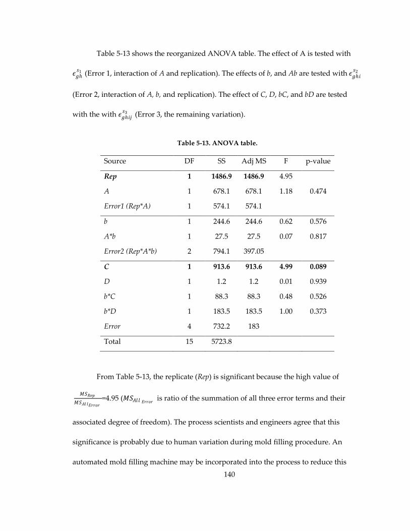
140
Table 5-13 shows the reorganized ANOVA table. The effect of A is tested with
𝜖𝑔𝑠1 (Error 1, interaction of A and replication). The effects of b, and Ab are tested with 𝜖𝑔𝑖
𝑠2
(Error 2, interaction of A, b, and replication). The effect of C, D, bC, and bD are tested
with the with 𝜖𝑔𝑖𝑗𝑠3 (Error 3, the remaining variation).
Table 5-13. ANOVA table.
Source DF SS Adj MS F p-value
Rep 1 1486.9 1486.9 4.95
A 1 678.1 678.1 1.18 0.474
Error1 (Rep*A) 1 574.1 574.1
b 1 244.6 244.6 0.62 0.576
A*b 1 27.5 27.5 0.07 0.817
Error2 (Rep*A*b) 2 794.1 397.05
C 1 913.6 913.6 4.99 0.089
D 1 1.2 1.2 0.01 0.939
b*C 1 88.3 88.3 0.48 0.526
b*D 1 183.5 183.5 1.00 0.373
Error 4 732.2 183
Total 15 5723.8
From Table 5-13, the replicate (Rep) is significant because the high value of
𝑀𝑆𝑅𝑒𝑝
𝑀𝑆𝐴𝑙 𝑙𝐸𝑟𝑟𝑜𝑟=4.95 (𝑀𝑆𝐴𝑙𝑙 𝐸𝑟𝑟𝑜𝑟 is ratio of the summation of all three error terms and their
associated degree of freedom). The process scientists and engineers agree that this
significance is probably due to human variation during mold filling procedure. An
automated mold filling machine may be incorporated into the process to reduce this

141
variation.
At the 10% significant level, the effect C (immersion time) is also significant (𝑝-
value = 0.089). The immersion time at 2 hrs provides a higher yield, whereas normally
the process engineers expect the yield to improve with longer times. A further
investigation into the diffusion of water and ethanol into the gelled particle matrix
should be carried out to fully understand and explain this effect.
Since the original objective of this project is to study the effect of interaction of
noise factor (b) and controllable factor (A, C, and D), as well as its interaction with other
controllable factors. From the ANOVA, it indicates that those effects are not significant.
Therefore, we decided to set the milling temperature at 10°C, the emersion time at 2
hours, the drying rate at normal, and the solid volume at 45%.
Although the milling temperature (noise factor) is not significant, it suggests that
the current LMRIF process is robust to the change in milling temperature; further
investment of milling temperature controller in full scale manufacturing might be
declined.

142
Yie
ld o
f Fo
rce
ps
4540
40
35
30
25
20
3010 42
SlowNormal
40
35
30
25
20
21
A b C
D Rep
Figure 5-3. Main Effect Plots, only C and Rep are significant.
If this experiment is analyzed based on completely randomized, its ANOVA
table is shown in Table 5-14. None are significant at 10% significant level, except
replication. If this analysis is used, the importance of the immersion time is probably
ignored.
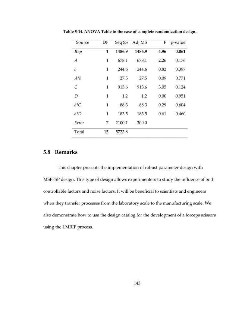
143
Table 5-14. ANOVA Table in the case of complete randomization design.
Source DF Seq SS Adj MS F p-value
Rep 1 1486.9 1486.9 4.96 0.061
A 1 678.1 678.1 2.26 0.176
b 1 244.6 244.6 0.82 0.397
A*b 1 27.5 27.5 0.09 0.771
C 1 913.6 913.6 3.05 0.124
D 1 1.2 1.2 0.00 0.951
b*C 1 88.3 88.3 0.29 0.604
b*D 1 183.5 183.5 0.61 0.460
Error 7 2100.1 300.0
Total 15 5723.8
5.8 Remarks
This chapter presents the implementation of robust parameter design with
MSFFSP design. This type of design allows experimenters to study the influence of both
controllable factors and noise factors. It will be beneficial to scientists and engineers
when they transfer processes from the laboratory scale to the manufacturing scale. We
also demonstrate how to use the design catalog for the development of a forceps scissors
using the LMRIF process.

144
Chapter 6.
Conclusion
This research addresses the challenges in the statistical modeling and analysis
that arise during the development of a small-scale forceps instrument for minimally
invasive surgery (MIS) using the lost mold rapid infiltration forming (LMRIF)
manufacturing process. Section 6.1 presents the summary of this research. Section 6.2
presents the research contributions; and Section 6.3 provides future work. Finally, the
broader impact of this research is given in Section 6.4.
6.1 Summary
Chapter 1 provides our research motivations which centered around the
development of a micro/nano-scale forceps scissors for minimally invasive surgery. A
brief introduction of the lost mold rapid infiltration forming (LMRIF) process is given.
The important characteristics of the LMRIF process lead to the need for the development
of a new class of experimental design—multistage fractional factorial split plot
(MSFFSP) design.
Chapter 2 reviews how design of experiments can be used as a tool for the
advancement of nanotechnology and nanomanufacturing. We found that the one-factor-
at-a-time approach is widely used in this area. Other traditional methods found are
factorial design, fractional factorial design, and response surface methodology.

145
However, most of these designs do not take the randomization principle into
consideration. We then suggested several modern DOE methods appropriate for
development in this area.
Chapter 3 discusses multistage fractional factorial split-plot (MSFFSP)
experiments. The LMRIF process conducted over three stages was studied and some
properties and characteristics of the MSFFSP structure were presented. These multistage
designs overcome the severe limitations of the commonly used factorial designs by
providing greater flexibility in the choice of confounding patterns. In addition, the
multistage designs require fewer runs than split-plot designs, while yielding greater
information about the factors of interest.
In Chapter 4, we focus on finding the optimal MSFFSP designs for multistage
experimentation. The algorithm to search for the optimal MSFFSP is developed and
coded in MATLAB with an example using the LMRIF process. Design catalogs for three
stage and four stage experiments is also presented. The catalogs will help experimenters
to choose an appropriate design so that the maximum amount of important information
can be drawn from their experimental effort.
In Chapter 5, we integrate the concept of the robust parameter design (RPD) into
the MSFFSP design. This type of design allows us to reduce variations in the product
and process. We also modify an algorithm to search for an optimal design for robust
study purposes. Some catalog designs are also presented with the demonstration in the
LMRIF process.

146
In summary, using these designs and integrating them into the modeling and
production for nanomanufacturing research will yield strategic advantages by
accelerating the research and development cycle, stretching the experimental budget,
and helping to create more reliable, robust, and better performing products.
6.2 Research Contribution
To facilitate experimentation in nanotechnology and nanomanufacturing,
multistage fractional factorial split-plot (MSFFSP) designs carried out over multiple
stages are proposed for process and product development. These designs are valuable to
experimenters in situations where some experimental units need to be treated over all
stages. These types of designs overcome the important assumption of the statistical
design of experiment; complete randomization. Using the split-plot, split-block, or a
combination of the two provides flexibility in experimentation by relaxing this
assumption. Other advantages of MSFFSP design include a reduction in the number of
settings and in the number of runs required for experimentation.
In addition, when transitioning from a laboratory setting to a real manufacturing
system, the expected results are often reversed due to changes in noise factors.
Therefore, we also integrated the concept of robust parameter design with multistage
experimentation to help experimenters to foresee problems and be prepared for mass
production.
Several catalog designs for three and four stage experimentation and two stage

147
experimentation with RPD are provided. Software code for determining design catalogs
for higher numbers of stages and higher numbers of factors is also provided.
Furthermore, we successfully demonstrate the use of MSFFSP design in the
important application of developing a forceps scissors using the LMRIF process. This
demonstration should also indicate that this type of design can be used in other types of
manufacturing processes in other fields.
6.3 Future work
We believe that as advanced nanotechnology and nanomanufacturing
applications are explored with experimental design, there will be new questions that call
for modifications, or perhaps completely new constructs, of experimental designs. This
will not only advance the field of DOE, but also amplify the potential of quality
methodologies that can be extended to other emerging areas. Specific directions of
future work are discussed below.
6.3.1 Integration of DOE and Reliability Study
Reliability is defined as the probability that a product can be used for a specific
amount of time without failure, given a specific design condition (Elsayed, 1996,
Elsayed, 2000). Reliability is one of the crucial characteristics of quality. However,
reliability is difficult to monitor and control for new products because it can only be
directly evaluated when the product has been on market for a certain period of time.

148
Therefore, we can only rely on indirect measures of reliability based on laboratory
testing.
Some recent challenges to improving the reliability of new products, particularly
at small scales, include instrumentation limitations and evolving standards. This,
coupled with the previously discussed manufacturing challenges at the micro and nano
scales, suggests that what is needed is the integration of experimental design and
reliability. This approach, with its potential as well as difficulties, has been discussed to
some extent in the literature (Hamada, 1995, Meeker and Hamada, 1995, Condra, 2001).
One of the main issues stems from the difference in characteristics between the product
quality and product reliability -- the former does not depend on the passage of time
while the latter does (Leemis, 1995).
We note, however, that the earlier work pertains to the case of a completely
randomized (CR) design. Therefore, there is a need to modify the experimental model to
accommodate the reliability data when the split-plot design is used with an accelerating
testing (AT) model with a restriction on randomization. The AT model allows
experimenters to obtain the reliability data quickly when the ‚harder-than-usual‛
conditions are applied to experimental units during testing. We believe that this
integration will address several challenges associated with the MIS development.
The idea behind the integration is to add the reliability testing (a factor) at the
final stage of experimentation where the set of final products from the different
treatment combinations will be regrouped and randomly tested under the same testing

149
conditions. This situation is similar to split-block structure.
Unlike data from general experimental design, the data from reliability study is
not normally distributed and nonnegative (i.e, life time data, number of cyclic loads
before failure), and they tend to be censored (Wu and Hamada, 2000). To incorporate
with the reliability data, two tasks need to be further explored for the MSFFSP design for
reliability: estimation problems with the censored data and the analysis of reliability
data.
6.3.2 Other Criteria for Optimal Design
In this research, we developed the optimal MSFFSP design based on maximum
resolution and minimum aberration which are considered to be broad applications
(Kulahci et al., 2006). It is also necessary to develop the design based on experimenters’
specific interest. Kulahci et al. (2006) points out that there are other important criteria
such as the maximum number of clear main effects, and maximum number of clear two-
factor interaction effects for fractional factorial split-plot design.
Therefore, it is necessary to develop an algorithm to set up the design catalog
based on the criteria for MSFFSP design. We believe that it would be more appropriate
to not create a design based on a single criterion. The design catalog with several criteria
may provide a benefit to experimenters. Then these criteria will also be modified for
robust parameter designs.

150
6.3.3 Different Design Structures in Each Stage
In this research, we only considered a single type of experimental design: the
two-level fractional factorial designs. This design is used primarily for screening
proposes. However, to study the process optimization, the structure for each stage may
be changed to be a more appropriate type of design, for example, central composite
design (CCD), or Box-Behnkin design (BBD). Vining et al. (2005) shows how to use CCD
to facilitate an experiment with split-plot structure.
Another type of design structure that may be used as MSFFSP design is saturated
or super-saturated designs. These designs are used when the number of runs is small
compared to the number of interested factors. Lin (1993) proposes a new class of
supersaturated designs using half fractions of Hadamard matrices. An MSFFSP design
combined with a supersaturated design may be another alternative to experimenters in
the case that the focus of the experiments is only on the main effects.
6.3.4 Sequential and Multiple Responses for MSFFSP Design
As in the real application of the LMRIF process, there are multiple output
responses. These are not only outputs at the final stage, but also outputs from different
stages. Figure 6-1 shows outputs after colloid preparation (particle size and particle
distribution), colloid deposition (% green-state yield and green strength), and sintering
(% fired yield and strength) of the LMRIF process. The experiment’s design and analysis
becomes much more complicated than with a single response; therefore, it is necessary
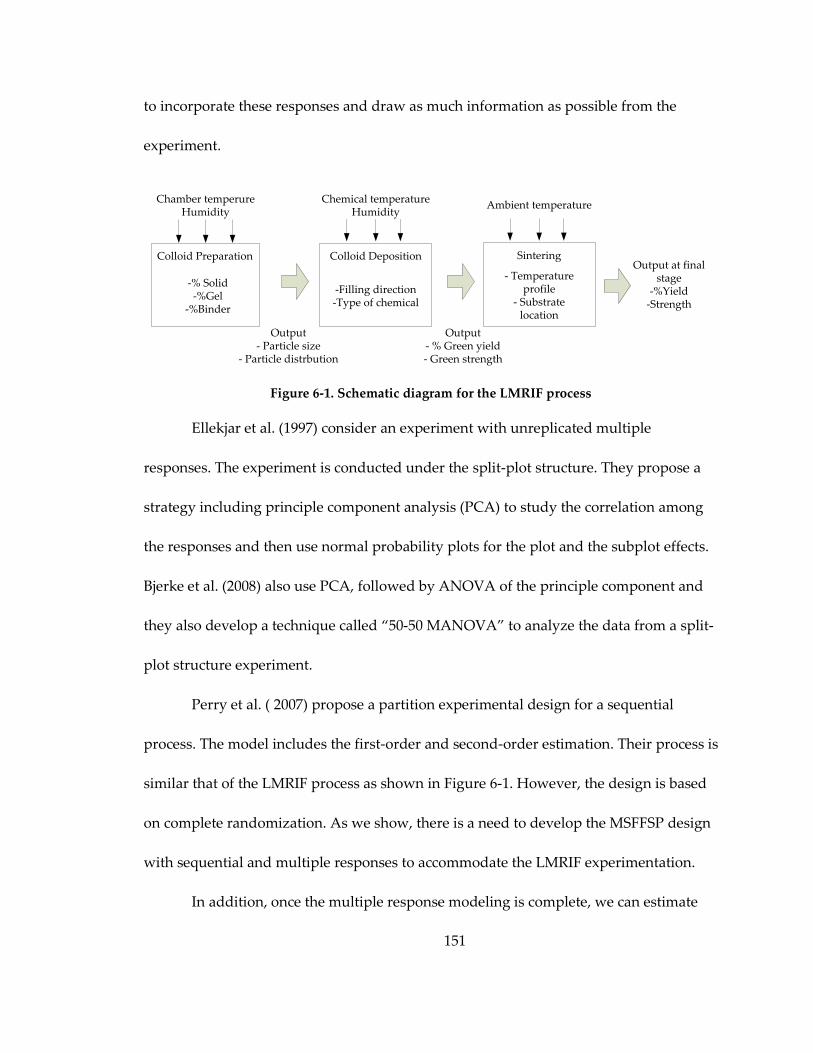
151
to incorporate these responses and draw as much information as possible from the
experiment.
-% Solid-%Gel
-%Binder
Colloid Preparation
-Filling direction-Type of chemical
Colloid Deposition
Chamber temperureHumidity
Chemical temperatureHumidity
Output at final stage
-%Yield-Strength
Output- Particle size
- Particle distrbution
- Temperature profile
- Substrate location
Sintering
Ambient temperature
Output- % Green yield- Green strength
Figure 6-1. Schematic diagram for the LMRIF process
Ellekjar et al. (1997) consider an experiment with unreplicated multiple
responses. The experiment is conducted under the split-plot structure. They propose a
strategy including principle component analysis (PCA) to study the correlation among
the responses and then use normal probability plots for the plot and the subplot effects.
Bjerke et al. (2008) also use PCA, followed by ANOVA of the principle component and
they also develop a technique called ‚50-50 MANOVA‛ to analyze the data from a split-
plot structure experiment.
Perry et al. ( 2007) propose a partition experimental design for a sequential
process. The model includes the first-order and second-order estimation. Their process is
similar that of the LMRIF process as shown in Figure 6-1. However, the design is based
on complete randomization. As we show, there is a need to develop the MSFFSP design
with sequential and multiple responses to accommodate the LMRIF experimentation.
In addition, once the multiple response modeling is complete, we can estimate

152
the variability from the each stage and use this information for the implementation of
statistical process control and adjustment when the process is transferred to the
manufacturing scale.
6.3.5 MSFFSP Design and Analysis with Gage Repeatability and
Reproducibility
The gage repeatability and reproducibility (R&R) also plays a fundamental role
in the process improvement. It refers to a methodology used to identify and quantify the
source of variation during product measurement once the variability is determined.
Process engineers assess whether or not the measurement system is qualified to be used.
Although gage GR&R studies have been used for a long time, little research has
focused on how to conduct and analyze gage R&R based on split-plot structure (Burdick
et al., 2005). To demonstrate the application of the MSFFSP design and analysis, we will
apply the MSFFSP design to the gage R&R analysis on the optical microscope that used
to measure the dimension of small-scaled parts.
6.4 Broader Impact
Although the DOE have been used for decades, it is not used much in the areas
of nanotechnology and nanomanufacturing (Lu et al., 2009, Yuangyai and Nembhard,
2009). The key benefit of using DOE is to understand the relationship among existing or
new system parameters. This speeds up to the new product development process. In this

153
research, we develop a new class of experimental design, MSFFSP design, to overcome
physical difficulties during conducting an experiment. This MSFFSP design is a
fundamental concept that can potentially be integrated with other quality engineering
tools. The potential areas, as shown in our future work, include reliability study, robust
parameter, sequential and multiple responses, statistical process control and adjustment,
and gage R&R.
Significant advancements in these areas would revolutionize the use of quality
engineering tools. We believe also that the MSFFSP design can be used in other areas of
nanotechnology or nanomanufacturing processes, such as nanocoating, nanopowder,
sol-gel processes, self assembly processes, chemical vapor deposition processes, and
electro-deposition processes.
Nanotechnology and nanomanufacturing are multidisciplinary fields. For
example, the forceps scissors development presented in this research is a collaboration
among several science and engineering fields, including material science and
engineering, mechanical engineering, industrial engineering, and applied statistics.
From this involvement, we have explored some challenges of using DOE in
nanomanufacturing. This research directly and indirectly supports the cross-fertilization
of ideas from different disciplines and the systematic flow of information and people
among research groups. We hope that this kind of collaboration will address several
more challenges in nanotechnology and nanomanufacturing.
154
References
Acharya, N. and Lin, D. K. (2008). "Understanding a ZnO Nanorods Fabrication
Process," International Journal of Nanomanufacturing, Vol. 2, pp. 319-330.
Acharya, N. and Nembhard, H. B. (2008). "Statistical Design and Analysis for a Three-
Step Surface Initiated Polymerization Process," International Journal of
Nanomanufacturing, Vol. 2, pp. 331-345.
Aguirre, M. E., Frecker, M. and Nembhard, H. B. (2008a). "A Case Study Comparison of
Alternative Meta-Modelling Methods," International Journal of Nanomanufacturing,
Vol. 2, pp. 375-405.
Aguirre, M. E., Hayes, G., Frecker, M., Adair, J. and Antolino, N. (2008b). "Fabrication
and Design of A Nanoparticulate Enabled Micro Forceps," Proceeding of the
IDETC/CIE 2008, New York City, NY, USA.
Aguirre, M. E., Hayes, G., Yuangyai, C., Frecker, M., Adair, J. and Antolino, N. (2009).
"Fabrication and Strength-Based Design of A Meso Forceps," Proceeding of the
IDETC/CIE 2009, San Diego, CA, USA.
Anderson, M. J. and Whitcomb, P. J. (2005). RSM Simplified: Optimizing Process Using
Response Surface Methods for Design of Experiments, New York: Productivity Press.
Antolino, N. E., Hayes, G., Kirkpatrick, R., Muhlstein, C. L., Frecker, M. I.,
Mockensturm, E. M. and Adair, J. H. (2009a). "Lost Mold Rapid Infiltration
Forming of Mesoscale Ceramics: Part 1, Fabrication," Journal of American Ceramic
Society, Vol. 92, pp. S63-S69.
155
Antolino, N. E., Hayes, G., Kirkpatrick, R., Muhlstein, C. L., Frecker, M. I.,
Mockensturm, E. M. and Adair, J. H. (2009b). "Lost Mold Rapid Infiltration
Forming of Mesoscale Ceramics: Part 2, Geometry and Strength Improvements,"
Journal of American Ceramic Society, Vol. 92, pp. S70-S78.
Barglik-Chory, C., Remenyi, C., Strohm, H. and Miller, G. (2004). "Adjustment of the
Band Gap Energies of Biostabilized CdS Nanoparticles by Application of
Statistical Design of Experiments," J. Phys Chem. B, Vol. 108, pp. 7637-7640.
Basumallick, A., Das, G. C. and Mukherjee, S. (2003). "Design of Experiments for
Synthesizing in situ Ni-SiO2 and Co-SiO2 Nanocomposites by Non-isothermal
Reduction Treatment," Nanotechnology, Vol. 4, pp. 903-906.
Bingham, D. and Sitter, R. (1999). "Minimum Aberration Two-Level Fractional Factorial
Split-Plot Designs.," Technometrics, Vol. 41, pp. 62-70.
Bingham, D. and Sitter, R. (2001). "Design Issues in Fractional Factorial Split-Plot
Experiments," Journal of Quality Technology, Vol. 33, pp. 2-15.
Bingham, D. and Sitter, R. (2003). "Fractional Factorial Split-Plot Design for Robust
Parameter Experiments," Technometrics, Vol. 45, pp. 80-89.
Bisgaard, S. (2000). "The Design and Analysis of 2k-p x 2q-r Split-Plot Experiments," Journal
of Quality Technology, Vol. 32, pp. 39-56.
Bisgaard, S. and Steinberg, D. M. (1997). "The Design and Analysis of 2k-p x s prototype
Experiments," Technometrics, Vol. 39, pp. 52-62.
Bjerke, F., Langsrud, and Aastveit, A. H. (2008). "Restricted Randomization and

156
Multiple Responses in Industrial Experiments," Quality and Reliability Engineering
International, Vol. 24, pp. 167-181.
Box, G. and Jones, S. (2000-01). "Split Plots for Robust Product and Process
Experimentation," Quality Engineering, Vol. 13, pp. 127-134.
Box, G. E. P. (2006). Improving Almost Anything: ideas and essays, New Jersey: Wiley-
Interscience.
Box, G. E. P. and Anderson, S. L. (1955). "Permutation Theory in the Derivtion of Robust
Criteria and the Study of Departures from Assumption," Journal of the Royal
Statistical Society, Series B, Vol. 17, pp. 1-34.
Box, G. E. P. and Draper, N. R. (2007). Response Surfaces, Mixtures, and Ridge Analyses:
Wiley - Interscience.
Box, G. E. P. and Hunter, J. S. (1961). "The 2k-p Fractional Factorial Designs Part 1,"
Technometrics, Vol. 3, pp. 311-351.
Box, G. E. P., Hunter, J. S. and Hunter, W. G. (2005). Statistics for Experimenters: Design,
Innovation, and Discovery, New Jersey: John Wiley & Sons.
Burdick, R. K., Borror, C. M. and Montgomery, D. C. (2005). Design and Analysis of Gauge
R&R Studies, Philadelphia: ASA-Siam
Butler, N. A. (2004). "Construction of Two-Level Split-lot Fractional Factorial Designs for
Multistage Processes," Technometrics, Vol. 46, pp. 445-451.
Buzea, C., Beydaghyan, G., Elliott, C. and Robbie, K. (2005). "Control of Power Law
Scalling in the Growth of Silicon Nanocolumn Pseudo-Regular Arrays Deposited

157
by Glancing Angle Deposition," Nanotechnology, Vol. 16, pp. 1986-1992.
Cappelleri, D. J., Frecker, M. I., Simpson, T. W. and Snyder, A. (2002). "Design of a PZT
Bimorph Actuator Using a Metamodel-Based Approach," Transactions of the
ASME, Vol. 124, pp. 354-357.
Carrion, H., Rogosky, M., Nembhard, H. B., Joshi, S. and Catchmark, J. M. (2008).
"Characterization of the SilSpin Etch-Back ( breakthrough) Process for
Nanolithography with CHF3 and O2 Chemistry," International Journal of
Nanomanufacturing, Vol. 4, pp. 305-318.
Chang, H., Jwo, C. S., Lo, C. H. and Pai, S. H. (2007). "A Study of Process Optimization
Using the Combined Submerged Arc Nanoparticle Synthesis System for
Preparing TiO2," Journal of Alloys and Compounds, Vol. 434/435, pp. 668-671.
Charles, A., Chandon, Y., Bergeret, F. and Garcia, L. (1996). "Photolithography
Equipment Control through D-Optimal Design," Proceeding of SPIE-The
International Society of Optical Engineering,
Chen, C.-H., Wang, S.-J., Ko, R.-M., Kuo, Y.-C., Uang, K.-M., Chen, T.-M., Liou, B.-W.
and Tsai, H.-Y. (2006a). "The Influence of Oxygen Content in the Sputtering Gas
on the Self-synthesis of Tungsten Oxide Nanowires on Sputter-deposited
Tungsten Films," Nanotechnology, Vol. 17, pp. 217-223.
Chen, C., Wang, L., Jiang, G., Yang, Q., Wang, J., Yu, H., Chen, T., Wang, C. and Chen,
X. (2006b). "The Influence of Seeding Conditions and Shielding Gas Atmosphere
on the Synthesis of Silver Nanowires through the Polyol Process,"
158
Nanotechnology, Vol. 17, pp. 466-474.
Chen, J. and Lin, D. K. J. (1991). "On the Identity Relationships of 2k-p Designs," Journal of
Statistical Review, Vol. 61, pp. 131-145.
Chen, J., Sun, D. X. and Wu, C. F. J. (1993). "A Catalogue of Two-Level and Three-Level
Fractional Factorial Designs With Small Runs," International Statistical Review,
Vol. 61, pp. 131-145.
Chuang, H.-Y., Tsai, H.-K. and Kao, C.-Y. (2004). "Optimal Designs for Microarray
Experiments," Proceeding of the 7th International Symposium on Parallel
Architectures, Algorithms and Networks (ISPAN'04),
Clarke, S. M., Griebsch, J. H. and Simpson, T. W. (2005). "Analysis of Support Vector
Regression for Approximation of Complex Engineering Analyses," Journal of
Mechanical Design, Vol. 127, pp. 1077-1087.
Condra, L. W. (2001). Reliability Improvement with Design of Experiments, New York:
Marcel Dekker.
Daniel, C. (1973). "One-at-a-time Plans," Journal of American Statistical Association, Vol. 68,
pp. 353-360.
Desai, S., Mohan, R., Sankar, J. and Tiano, T. (2008). "Understanding Conductivity of
Single Wall Nanotubes (SWNTs) in a Composite Resin Using Design of
Experiments," International Journal of Nanomanufacturing, Vol. 2, pp. 292-304.
Dimaki, M. and Boggild, P. (2005). "Frequency Dependence of the Structure and
Electrical Behaviour of Carbon Nanotube Networks Assembled by
159
Dielectrophoresis," Nanotechnology, Vol. 16, pp. 759-763.
Doumanidis, H. (2001). "The Nanomanufacturing Programme at the National Science
Foundation," Nanotechnology, Vol. 13, pp. 248-252.
Elsayed, E. A. (1996). Reliability Engineering, Reading, MA: Addison Wesley Longman.
Elsayed, E. A. (2000). "Perspectives and Challenges for Research in Quality and
Reliability," International Journal of Production Research, Vol. 38, pp. 1953-1976.
Federer, W. T. and King, F. (2007). Variations on Split Plot and Split Block Experiment
Designs, New Jersey: Wiley-Interscience
Fisher, R. A. (1966). The Design of Experiments, Edinburgh: Oliver and Boyd.
Franklin, M. F. (1984). "Constructing Tables of Minimum Aberration pn-m Designs,"
Technometrics, Vol. 26, pp. 225-232.
Franklin, M. F. and Bailey, R. A. (1977). "Selecting Defining Contrasts and Confouned
Effects in Two-Level Experiments," Applied Statistics, Vol. 26.
Franklin, M. F. and Bailey, R. A. (1985). "Selecting Defining Contrasts and Confounded
Effects in pn-m Factorial Experiments," Technometrics, Vol. 27, pp. 165-172.
Frecker, M., Dziedzic, R. and Haluck, R. (2002). "Design of Multifunctional Compliant
Mechanisms for Minimally Invasive Surgery," Minimally Invasive Therapy and
Allied Technologies, Vol. 11, pp. 311-319.
Frecker, M., Schadler, J., Haluck, R., Culkar, K. and Dziedzic, R. (2005). "Multifunctional
Instruments for Laparoscopic Surgery: Design and Testing of Initial Prototypes,"
Journal of the Society of Laparoendoscopc Surgeons, Vol. 9, pp. 105-112.
160
Fries, A. and Hunter, W. G. (1980). "Minimum Aberration 2k-p Designs," Technometrics,
Vol. 22, pp. 601-608.
Giesbrecht, F. G. and Gumpertz, M. L. (2004). Planning, Construction, and Statistical
Analysis of Comparative Experiments, New Jersey: John Wiley & Sons.
Gou, J., Liang, Z. and Wang, B. (2004). "Experimental Design and Optimization of
Dispersion Process for Single-Walled Carbon Nanotube Bucky Paper,"
International Journal of Nanoscience, Vol. 3, pp. 293-307.
Gryna, F. M., Chua, R. and Defeo, J. A. (2007). Juran's Quality Planning and Analysis for
Enterprise Quality, Boston: McGraw Hill.
Hamada, M. (1995). "Using Statistically Designed Experiments to Improve reliability and
to Achieve Robust Reliability," IEEE Transactions on Reliability, Vol. 44, pp. 206-
215.
Hibino, H. and Kimura, K. (1988). Optical endoscope having image signal transmitting
cable.
Hinkelmann, K. and Kempthorne, O. (2008). The Design and Analysis of Experiments:
Volume 1 Introduction to Experimental Design, New Jersey: Wiley-Interscience.
Hooker, A. C., Foracchia, M., Dodds, M. G. and Vicini, P. (2003). "An Evaluation of
Population D-Optimal Designs Via Pharmacokinetic Simulation," Annals of
Biomedical Engineering, Vol. 31, pp. 98-111.
Hou, T.-H., Su, C.-H. and Liu, W.-L. (2007). "Parameter Optimization of a Nano-Particle
Wet Milling Process Using the Taguchi Method, Response Surface Method and

161
Genetic Algorithm," Powder Technology, Vol. 173, pp. 153-162.
http://isotc.iso.org/livelink/livelink/6356960/TC_229_BP_2007-
2008.pdf?func=doc.Fetch&nodeid=6356960, last access: November 16, 2007.
Huang, H., Tan, O. K., Lee, Y. C., Tse, M. S., Guo, J. and White, T. (2006). "Effects of
Plasma Treatment on the Growth of SnO2 Nanorods from SnO2 Thin Films,"
Nanotechnology, Vol. 17, pp. 743-746.
Huang, P., Chen, D. and Voelkel, J. (1997). "Minimum Aberration Two-Level Split-Plot
Designs," Technometrics, Vol. 40, pp. 314-326.
Hunter, W. G. (1999). Design and Analysis of Experiments. In: Juran, J. M. and Godfrey,
A. (Eds.) Juran's Quality Handbook. 5th ed., Collins.
International, A. (2002). ASTM C 1161-02c, "Standard Test Method for Flexural Strength
of Advanced Ceramics at Ambient Temperature".
Jeng, S. L., Lu, J. C. and Wang, K. (2007). "A Review of Reliability Research on
Nanotechnology," IEEE Transactions on Reliability, Vol. 56, pp. 401-410.
Juran, J. M. and Godfrey, A. (1999). Juran's Quality Handbook, New York: McGraw Hill.
Kempthorne, O. (1952). The Design and Analysis of Experiments: John Wiley
Kim, B., Park, N., Na, P. S., So, H.-M., Kim, J.-J., Kim, H., Kong, K.-J., Chang, H., Ryu, B.-
H., Choi, Y. and Lee, J.-O. (2006). "The Effect of Metal Cluster Coatings on
Carbon Nanotubes," Nanotechnology, Vol. 17, pp. 496-500.
Kim, T.-W., Wang, G., Lee, H. and Lee, T. (2007). "Statistical Analysis of Electronic
Properties of Alkanethiols in Metal-molecule-metal junction," Nanotechnology,
162
Vol. 18, pp. 1-8.
Kowalski, S. M. and Potcner, K. J. (2003). "How to Recognize a Split Plot Experiment,"
Quality Progress, Vol. 36, pp. 60-67.
Kubovecz, A., Mehn, D., Nemes-Nagy, E., Szabo, R. and Kiricsi, I. (2005). "Optimization
of CCVD Synthesis Conditions for Single-Wall Carbon Nanotubes by Statistical
Design of Experiments (DoE)," Carbon, Vol. pp. 2842-2849.
Kukovecz, A., Mehn, D., Nemes-Nagy, E., Szabo, R. and Kiricsi, I. (2005). "Optimization
of CCVD Synthesis Conditions for Single-Wall Carbon Nanotubes by Statistical
Design of Experiments (DoE)," Carbon, Vol. pp. 2842-2849.
Kulahci, M., Ramirez, J. G. and Tobias, R. (2006). "Split-Plot Fractional Designs: Is
Minimum Aberation Enough?," Journal of Quality Technology, Vol. 38, pp. 56-64.
Kumar, R., Antolino, N., Wichard, J. E., Sutovich, K. J., Chapman, D. M., Roberie, T. G.
and Adair, J. H. (2005). Optimized De-aggregation and Dispersion of High
Concentration Slurry of Nanophase Alumina by Chemically Aided Attrition
Milling. working paper.
Lee, W. and Liu, T.-Y. (2007). "The Effect of Annealing Temperature on the
Microstructure of Nanoidented Au/Cr/Si," Nanotechnology, Vol. 18, pp. 1-10.
Leemis, L. M. (1995). Reliability: Probabilistic Models and Statistical Methods: McGraw-Hill.
Li, J., Zhang, Q., Li, H. and Chan-Park, M. B. (2006). "Influence of Triton X-100 on the
Characteristics of Carbon Nanotube Filed-Effect Transistors," Nanotechnology,
Vol. 17, pp. 668-673.
163
Lin, D. K. J. (1993). "A New Class of Supersaturated Designs," Technometrics, Vol. 35, pp.
28-31.
Lin, D. K. J. (2003). Industrial Experimentation for Screening. In: Khattree, R. and Rao.,
C. R. (Eds.) Handbook of Statistics in Industry. New York, North-Holland.
Lindsey, J. K. (1999). Models for Repeated Measurements, New York: Oxford University
Press.
Lu, J.-C., Jeng, S.-L. and Wang, K. (2009). "A Review of Statistical Methods for Quality
Improvement and Control in Nanotechnology," Journal of Quality Technology, Vol.
41, pp. 148-164.
Mattila, M., Hakkarainen, T., Jiang, H., Kauppinen, E. I. and Lipsanen, H. (2007). "Effect
of Substrate Orientation on the Catalyst-free Growth of InP Nanowires,"
Nanotechnology, Vol. 18, pp. 1-5.
Mead, R. and Pike, D. J. (1975). "A Review of Response Surface Methodology from a
Biometric Viewpoint," Biometrics, Vol. pp. 803-851.
Meeker, W. Q. and Hamada, M. (1995). "Statistical Tools for the Rapid Development and
Evaluation of High-Reliability Products," IEEE Transactions on Reliability, Vol. 44,
pp. 187-197.
Montgomery, D. C. (1996). Introduction to Statistical Quality Control: John Wiley & Sons.
Montgomery, D. C. (2005). Design and Analysis of Experiments, New Jersey: John Wiley &
Sons.
Montgomery, D. C. (2009). Design and Analysis of Experiments, New Jersey: John Wiley &
164
Sons.
Mukerjee, R. and Wu, C. G. J. (2006). A Modern Theory of Factorial Designs, New York:
Springer.
Myers, R. H. and Montgomery, D. C. (2002). Response Surface Methodology: Process and
Product Optimization Using Desinged Experiments, New York: Wiley-Interscience.
Myers, R. H., Montgomery, D. C., Vining, G. G., Borror, C. M. and Kowalski, S. M.
(2004). "Response Surface Methodology: A Retrospective and Literature Survey,"
Journal of Quality Technology, Vol. 36, pp. 53-77.
Nair, V. N. (1992). "Taguchi's Parameter Design: A Panel Discussion," Technometrics, Vol.
34, pp. 127-161.
Nembhard, H. B. (2007). "Nanotechnology: A Big Little Frontier for Quality," Quality
Progress, Vol. pp. 23-29.
Nembhard, H. B., Acharya, N., Artan, M. and Kim, S. (2006). Design Issues and Analysis
of Experiments in Nanomanufacturing. Handbook of Industrial and Systems
Engineering.
Neter, J., Kutner, M. H., Nachtsheim, C. J. and Wasserman, W. (1990). Applied Linear
Statistical Models.
Nourbakhsh, A., Ganjipour, B., Zahedifar, M. and Arzi, E. (2007). "Morphology
Optimization of CCVD-synthesized Multiwall Carbon Nanotubes, Using
Statistical Design of Experiments," Nanotechnology, Vol. 18, pp. 1-7.
Page, A. L. (1993). "Assessing New Product Development Practices and Performance:
165
Estabilishing Crucial Norms," Journal of Product Innovation Management, Vol. 10,
pp. 273-290.
Pan, A., Lin, X., Liu, R., Li, C., He, X., Gao, H. and Zou, B. (2005). "Surface Crystallization
Effects on the Optical and Electric Properties of CdS Nanorods," Nanotechnology,
Vol. 16, pp. 2402-2404.
Panchapakesan, B., Cavicchi, R., Semancik, S. and DeVoe, D. L. (2006). "Sensitivity,
Selectivity and Stability of Tin Oxide Nanostructures on Large Area Arrays of
Microhotplates," Nanotechnology, Vol. 17, pp. 415-425.
Paniagua-Quinones, C. (2004). Use of Strip-block Designs for Multi-stage Processes to
Reduce Cost of Experimentation. Ph. D. Dissertation, Department of Industrial
Engineering. University of Wisconsin, Madison.
Perry, L. A., Montgomery, D. C. and Fowler, J. W. (2007). "A Partition Experimental
Design for a Sequential Process with a Large Number of variables," Quality and
Reliability Engineering International, Vol. 23, pp. 555-564.
Plank, H., Gspan, C., Dienstleder, M., Kothleitner, G. and Hofer, F. (2009). "The Influence
of Beam Defocus on Volume Growth Rates for Electron Beam Induced Platinum
Deposition," Nanotechnology, Vol. 19, pp. 1-9.
Quinones, M. d. C. P. (2004). Use of Strip-Block Designs for Multi-Stage Processes to
Reduce Cost of Experimentation. Industrial Engineering. Madison, University of
Wisconsin-Madison.
Rajaram, G., Desai, S., Xu, Z., Pai, D. M. and Sankar, J. (2008). "RSM-Based Optimization
166
for the Processing of Nanoparticulate SOFC Anode Material," International
Journal of Nanomanufacturing, Vol. 4, pp. 346-362.
Riddin, T. L., Gericke, M. and Whiteley, C. G. (2006). "Analysis of the Inter- and
Extracellular Formation of Platinum Nanoparticles by Fusarium Oxysporum f. sp.
lycopersici Using Response Surface Methodology," Nanotechnology, Vol. 17, pp.
3482-3489.
Roy, S. K., Dey, R., Mitra, A., Mukherjee, S., Mitra, M. K. and Das, G. C. (2007).
"Optimization of Process Parameters for the Synthesis of Silica Gel-WC
Nanocomposite by Design of Experiment," Materials Science and Engineering, Vol.
27, pp. 725-728.
Ryan, T. P. (2007). Modern Experimental Design, New Jersey: John Wiley & Sons.
Saravanan, P., Selvarajan, V., Joshi, S. V. and Sundrararajan, G. (2001). "Experimental
Design and Performance Analysis of Alumina Coatings Deposited by a
Detonation Spray Process," Journal of Physics D: Applied Physics, Vol. 34, pp. 131-
140.
Schneider, R., Wolpert, C., Guilloteau, H., Balan, L., Lambert, J. and Merlin, C. (2008).
"The Exposure of Bacteria to CdTe-core Quantum Dots: the Importance of
Surface Chemistry on Cytotoxicity," Nanotechnology, Vol. 20, pp. 1-10.
Schulte, J. (2005). Nanotechnology: Global Strategies, Industry Trends and Application: John
Willey.
Simpson, T. W., Mauery, T. M., Korte, J. J. and Mistree, F. (1998). "Comparison of
167
Response Surface and Kriging Models for Multidisciplinary Design
Optimization," AIAA Journal, Vol. pp. 1-11.
Stassen, H. G., Grimbergen, C. A. and Dankelman, J. (2005). Introduction to Minimally
Invasive Surgery. In: Dankelman, J., Grimbergen, C. A. and Stassen, H. G. (Eds.)
Engineering for Patent Safety: Issues in Minimally Invasive Procedures. New Jersey,
Lawrence Erlbaum.
Sun, Y., Zhang, Z. and Wong, C. P. (2005). "Study on Mono-Dispersed Nano-Size Silica
by Surface Modification for Underfill Applications," Journal of Colloid and Interface
Science, Vol. 292, pp. 436-444.
Taguchi, G. (1987). System of Experimental Design, New York: UNIPUB.
Taguchi, G., Chowdhury, S. and Taguchi, S. (1999). Robust Engineering: McGraw-Hill.
Taguchi, G., Chowdhury, S. and Wu, Y. (2005). Taguchi's Quality Engineering Handbook,
New Jersey: John Wiley & Son.
Unalan, H. E. and Chhowalla, M. (2005). "Investigation of Single-walled Carbon
Nanotube Growth Parameters Using Alcohol Catalytic Chemical Vapour
Deposition," Nanotechnology, Vol. 16, pp. 2153-2163.
Vinning, G. G., Kowalski, S. M. and Montgomery, D. C. (2005). "Response Surface
Designs Within a Split Plot Structure," Journal of Quality Technology, Vol. 37, pp.
115-129.
Vivacqua, C. and Bisgaard, S. (2004). "Strip-Block Experiments for Process Improvement
and Robustness," Quality Engineering, Vol. 16, pp. 495-500.

168
Vivacqua, C. A. and Bisgaard, S. (2009). "Post-Fractionated Strip-Block Designs,"
Technometrics, Vol. 51, pp. 47-55.
Wu, C. F. J. and Hamada, M. (2000). Experiments: Planning, Analysis, and Parameter Design
Optimization, New York: John Wiley & Sons.
Wu, C. F. J. and Zhu, Y. (2003). "Optimal Selection of Single Arrays for parameter design
experiments," Statistica Sinica, Vol. 13, pp. 1179-1199.
Wunderle, B. and Michel, B. (2006). "Progress in Reliability Research in the Micro and
Nano Region," Microelectronics Reliability Vol. 46, pp. 1685-1694.
Xue, K., Xu, J. B., Xi, L., An, J. and Chen, J. (2005). "In Situ Fabrication and
Characterization of Tungsten nanodots on SiO2/Si via Field Induced Nanocontact
with a Scanning Tunnelling Microscope," Nanotechnology, Vol. 16, pp. 2993-3000.
Yates, F. (1937). The Design and Analysis of Factorial Experiments, England: Imperial
Bureau of Social Science.
Yong, V. and Hahn, H. T. (2005). "Dispersant Optimization Using Design of Experiments
for SiC/Vinyl Ester Nanocomposites," Nanotechnology, Vol. 16, pp. 354-360.
Yuangyai, C. and Nembhard, H. B. (2009). Design of Experiments: A Key to Innovation
in Nanotechnology. In: Ahmed, W. and Jackson, M. J. (Eds.) Emerging
Nanotechnologies for Manufacturing. Burlington, William Andrew.
Yuangyai, C., Nembhard, H. B., Hayes, G., Antolino, N. and Adair, J. H. (2009). "Yield
Improvement for Lost Mold Rapid Infiltration Forming Process by a Multi-Stage
Fractional Factorial Split Plot Design," International Journal of Nanomanufacturing,

169
Vol. 3, pp. 351-367.
Zhang, T., Jin, C., Zhang, J., Lu, X., Qian, T. and Li, X. (2005). "Microstructure and
Magnetic Properties of Ordered La0.62Pb0.38MnO3 Nanowire Arrays,"
Nanotechnology, Vol. 16, pp. 2743-2747.

Vita
Chumpol Yuangyai has Bachelor's degree of Engineering in Mechanical
Engineering from the Prince of Songkla University, Thailand. After graduation, he had
joined the Siam Cement Group (SCG), one of the largest companies in Thailand, for ten
years. He began his professional at Siam Magotteaux as a quality engineer and then
production section manager. During his time at SCG, he was awarded a scholarship to
pursue his master’s degree in Industrial Engineering at the Asian Institute of
Technology, Thailand. Upon completion of his master’s degree, he worked at Thai CRT
Co. Ltd, a cathode ray tube manufacturer.
To broaden his knowledge; he decided to pursue a doctoral degree at
Department of Industrial and Manufacturing Engineering at The Pennsylvania State
University through the Laboratory for Quality Engineering and System Transitions
(QUEST) under the supervision of Dr. Harriet Black Nembhard. Upon completion of his
Ph.D., he currently works as a research associate at QUEST lab to further strengthening
his research skills. He will then take a professor position at Department of Industrial
Engineering, King Mongkut Institute of Technology, Ladkrabang, Thailand, where he
has been awarded a professorship from the Royal Thai Government.
He plans to continue building upon his work and leverage it for teaching and
improvement in industry in Thailand. He hopes that his skills and experiences in the
area of quality engineering will help him to become a strong advocate for global
manufacturing.


![PARAMETER-ROBUST DISCRETIZATION AND ...1507.03199v4 [math.NA] 21 Jun 2016 PARAMETER-ROBUST DISCRETIZATION AND PRECONDITIONING OF BIOT’S CONSOLIDATION MODEL JEONGHUN J. LEE, KENT-ANDRE](https://static.fdocuments.in/doc/165x107/5ae47a837f8b9a5d648f64af/parameter-robust-discretization-and-150703199v4-mathna-21-jun-2016-parameter-robust.jpg)