THESIS SUMMARY

Experimental and Numerical Study for Stress Experimental and Numerical Study for Stress Experimental and Numerical Study for Stress Experimental and Numerical Study for Stress

Measurement by Jack Fracturing and Estimation of Measurement by Jack Fracturing and Estimation of Measurement by Jack Fracturing and Estimation of Measurement by Jack Fracturing and Estimation of

Stress Distribution in Rock MassStress Distribution in Rock MassStress Distribution in Rock MassStress Distribution in Rock Mass

Presented by Dr. Gang Li

Civil and Environmental Engineering

Yamaguchi University

Attribution

2

This thesis comprises a series of three papers either published or under revision in journals. In

chronological order these papers are:

GANG LI, Y. MIZUTA, T. ISHIDA, O. SANO, 'Numerical Simulation of Performance Tests on a

New System for Stress Measurement by Jack Fracturing', Journal of the Mining and Materials

Processing Institute of Japan (MMIJ),Vol.121 (2005) No.9, 409-415.

C. LIU, GANG LI, K. KURIYAMA, Y. MIZUTA, 'Development of a Computer Program for

Inhomogeneous Modeling by 3D BEM with Analytical Integration and its Application to Rock

Slope Stability Evaluation', Int. J. Rock Mech. Min. Sci, Volume 42 (2005), 137-144.

GANG LI, Y. MIZUTA, T. ISHIDA, H. LI, S. Nakama, T. Sato, 'Stress Field Determination from

Local Stress Measurements by Numerical Modeling', Int. J. Rock Mech. Min. Sci, (under

revision).

Abstract

It is important to understand rock stress state in civil, mining, petroleum, earthquake engineering

and energy development, as well as in geophysics and geology. In general, however, estimating

the stress spatial distribution in rock is very difficult. The differences between the estimated and

the measured stresses can be first attributed to tectonic stresses, as well as other factors such as

topography and inhomogeneity of the rock mass. In this research, a study combining strategy and

tactics for the determination of in situ rock stress was undertaken to resolve difficulties and

improve accuracy of stress estimation. Numerical and experimental tests of a new borehole jack

fracturing probe by loading a steel pipe were carried out. On the other hand, an improved

computer program was developed available for inhomogeneous modeling and its applicability

was examined by comparing the numerical results with the corresponding strict solution. A non-

linear numerical inverse method is presented for evaluating the in situ state of stress in a rock

mass. The whole study is decomposed into the following chapters:

In chapter 1, at the first, the background of this study is introduced, including both in-situ and

numerical methods for rock stress estimation. At the second, the objectives and scope of the

study are explained, and finally the organization of the thesis is listed.

In chapter 2, a prototype probe for in-situ stress determination by borehole jack fracturing is

introduced and the following results are achieved:

(1) A new borehole jack single-fracture probe for deep stress measurements is developed. The

3

new probe includes unique borehole jack loading system and new special tangential strain

sensors to detect the opening of fractures directly.

(2) Loading tests of the new probe in a steel pipe is carried out to study stress distribution on

borehole surface induced by loading with the probe. The measurement data are compared with

the numerical results and they agree fairly well. Through the test and numerical results, it was

found that the probe generates high tensile stress concentration at the opening section where a

fracture is expected to be formed, and the stress concentration factor, k is 0.92. In the

longitudinal direction, the probe generates a relatively constant distribution of the tangential

stress within the scope of influence of the probe.

(3) The new developed borehole jack single-fracture probe presents the following advantages

over the previous hydraulic or sleeve fracturing techniques. Firstly, a fracture can be generated at

the intended direction based on the unique loading mechanism of the probe. Secondly,

inaccuracies aroused by dealing with fluid pressure distribution in the fracture are not expected

since no fluid is applied to the borehole wall. Thirdly, the opening of the fracture is measured

directly by the tangential strain sensor; therefore the re-opening pressure of the fracture can be

detected accurately.

In chapter 3, to consider the influence of tectonic stresses, topography and rock mass

inhomogeneity, the author has developed an improved procedure available for inhomogeneous

modeling and confirmed its validity by comparing the numerical results given by the procedure

with the corresponding strict solution. After that, the new procedure was applied to a stability

evaluation analysis of man-made rock slope, and it was confirmed that rock surface

displacements at the seven measuring points to date is due to elastic deformation based on

removal of overburden pressure by excavation progress – because of the agreement between the

displacements of the seven points which were calculated from the models of an inhomogeneous

elastic body and the displacements at the corresponding points, which were actually measured.

In chapter 4, using the inhomogeneous 3D BEM developed in the chapter 3, a new proposal

for the determination of the far field stresses based on stress measurement results is developed.

The 3D BEM applications with an introduction of 3D FDM have shown that the estimated

stresses agree well with the tendency of the in situ measurement data. It is likely that the tectonic

stresses have to be considered for a better estimation of underground stress distribution in

tectonically active region, such as in Japanese islands.

4

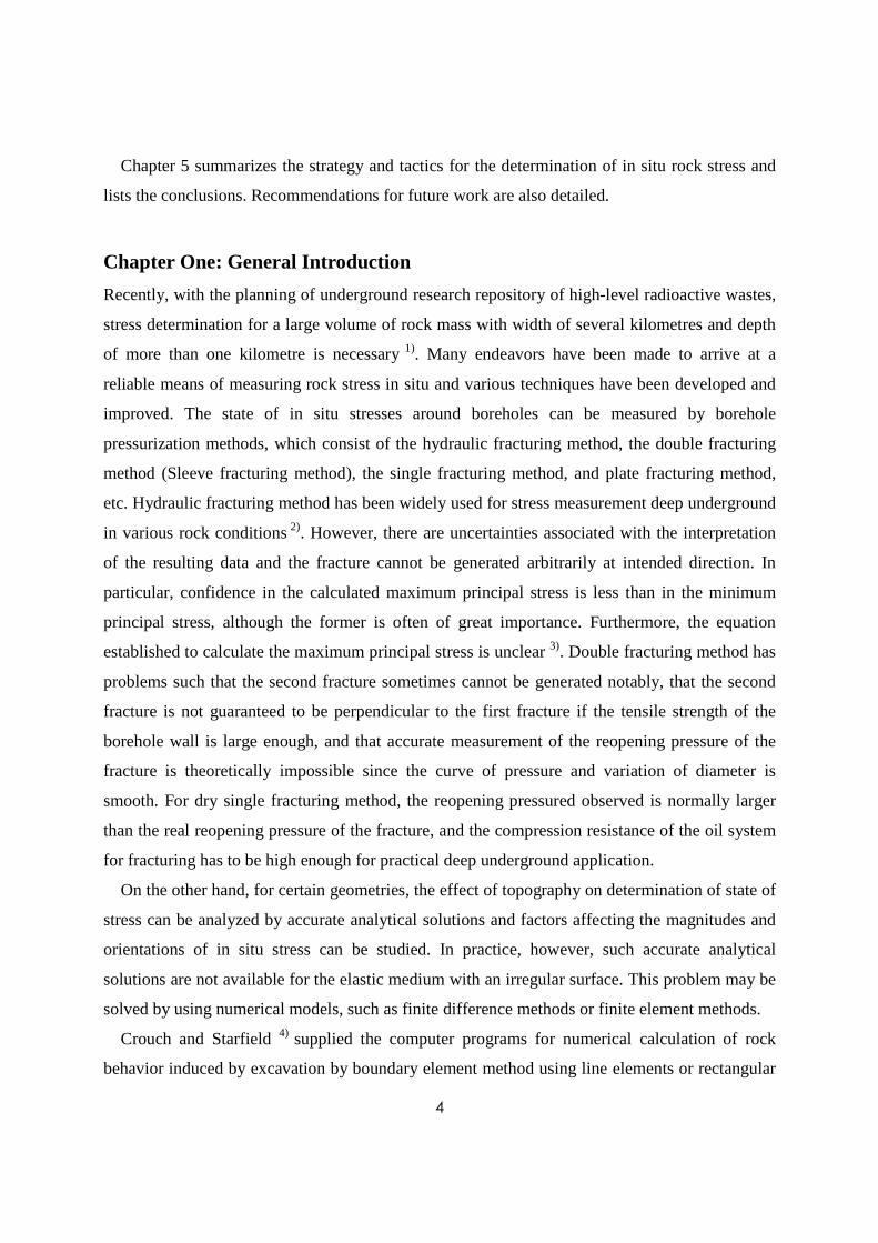
Chapter 5 summarizes the strategy and tactics for the determination of in situ rock stress and

lists the conclusions. Recommendations for future work are also detailed.

Chapter One: General Introduction

Recently, with the planning of underground research repository of high-level radioactive wastes,

stress determination for a large volume of rock mass with width of several kilometres and depth

of more than one kilometre is necessary 1). Many endeavors have been made to arrive at a

reliable means of measuring rock stress in situ and various techniques have been developed and

improved. The state of in situ stresses around boreholes can be measured by borehole

pressurization methods, which consist of the hydraulic fracturing method, the double fracturing

method (Sleeve fracturing method), the single fracturing method, and plate fracturing method,

etc. Hydraulic fracturing method has been widely used for stress measurement deep underground

in various rock conditions 2). However, there are uncertainties associated with the interpretation

of the resulting data and the fracture cannot be generated arbitrarily at intended direction. In

particular, confidence in the calculated maximum principal stress is less than in the minimum

principal stress, although the former is often of great importance. Furthermore, the equation

established to calculate the maximum principal stress is unclear 3). Double fracturing method has

problems such that the second fracture sometimes cannot be generated notably, that the second

fracture is not guaranteed to be perpendicular to the first fracture if the tensile strength of the

borehole wall is large enough, and that accurate measurement of the reopening pressure of the

fracture is theoretically impossible since the curve of pressure and variation of diameter is

smooth. For dry single fracturing method, the reopening pressured observed is normally larger

than the real reopening pressure of the fracture, and the compression resistance of the oil system

for fracturing has to be high enough for practical deep underground application.

On the other hand, for certain geometries, the effect of topography on determination of state of

stress can be analyzed by accurate analytical solutions and factors affecting the magnitudes and

orientations of in situ stress can be studied. In practice, however, such accurate analytical

solutions are not available for the elastic medium with an irregular surface. This problem may be

solved by using numerical models, such as finite difference methods or finite element methods.

Crouch and Starfield 4) supplied the computer programs for numerical calculation of rock

behavior induced by excavation by boundary element method using line elements or rectangular

5

leaf elements. They include Fictitious Stress Method (FSM) and Displacement Discontinuity

Method (DDM) by Indirect Method, and Direct Boundary Integral Method. The Indirect

Methods were extended to three-dimensional procedures using triangular leaf elements by

Kuriyama & Mizuta 5) and Kuriyama et al 6). However, there was some restriction in procedure

of boundary division in elements because one cannot place the center of gravity of any element

on the elongation of any side of any other triangular element. After that, however, such problem

has been resolved mathematically 7), but it has been still for homogeneous modeling.

Chapter Two: Experiment and Numerical Simulation on a New System for

Stress Measurement by Jack Fracturing

Probe for the borehole jack single-fracture method

The borehole jack single-fracture probe mainly consists of eight loading jacks, upper and lower

load platens, two pairs of friction shells, and two tangential strain sensors. The eight borehole

jack cylinders are grouped into upper section and lower section corresponding to the respective

loading platens and friction shells, and thus each section consists of four borehole jack cylinders.

Fig.1 shows the photo of the borehole jack probe used for the borehole whose diameter is 98 mm.

The probe is 676 mm in length and 96.6 mm in diameter.

Fig.1 Outward appearance of the borehole jack probe (676 mm in length and 96.6 mm in diameter) used for φ98 borehole

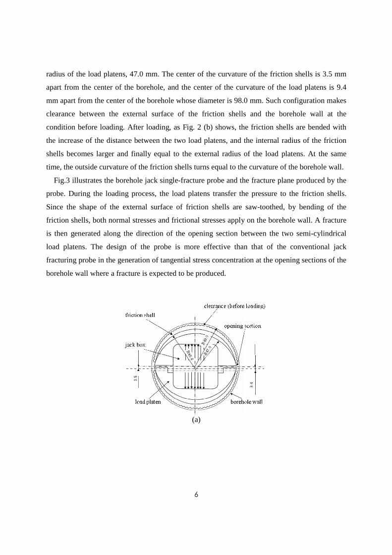
The cross section view of the probe is shown in Fig.2. Semi-cylindrical load platens of the

probe are covered by two pairs of half-pipe shaped friction shells. Before loading as shown in

Fig. 2(a), the internal radius of the friction shells is 45.6 mm and it is smaller than the external

6

radius of the load platens, 47.0 mm. The center of the curvature of the friction shells is 3.5 mm

apart from the center of the borehole, and the center of the curvature of the load platens is 9.4

mm apart from the center of the borehole whose diameter is 98.0 mm. Such configuration makes

clearance between the external surface of the friction shells and the borehole wall at the

condition before loading. After loading, as Fig. 2 (b) shows, the friction shells are bended with

the increase of the distance between the two load platens, and the internal radius of the friction

shells becomes larger and finally equal to the external radius of the load platens. At the same

time, the outside curvature of the friction shells turns equal to the curvature of the borehole wall.

Fig.3 illustrates the borehole jack single-fracture probe and the fracture plane produced by the

probe. During the loading process, the load platens transfer the pressure to the friction shells.

Since the shape of the external surface of friction shells are saw-toothed, by bending of the

friction shells, both normal stresses and frictional stresses apply on the borehole wall. A fracture

is then generated along the direction of the opening section between the two semi-cylindrical

load platens. The design of the probe is more effective than that of the conventional jack

fracturing probe in the generation of tangential stress concentration at the opening sections of the

borehole wall where a fracture is expected to be produced.

(a)

7

(b)

Fig.2 Cross section view of the probe: (a) before loading (b) after loading

Fig.3 Illustration for stress measurement by the borehole jack single-fracture probe

The upper section and lower section of the borehole jack cylinders are grouped in such a way

as to leave a small 30 mm wide gap in the centre of the probe. The gap shown in Fig. 1

accommodates a pair of new specific tangential strain sensors that are applied on opposite sides

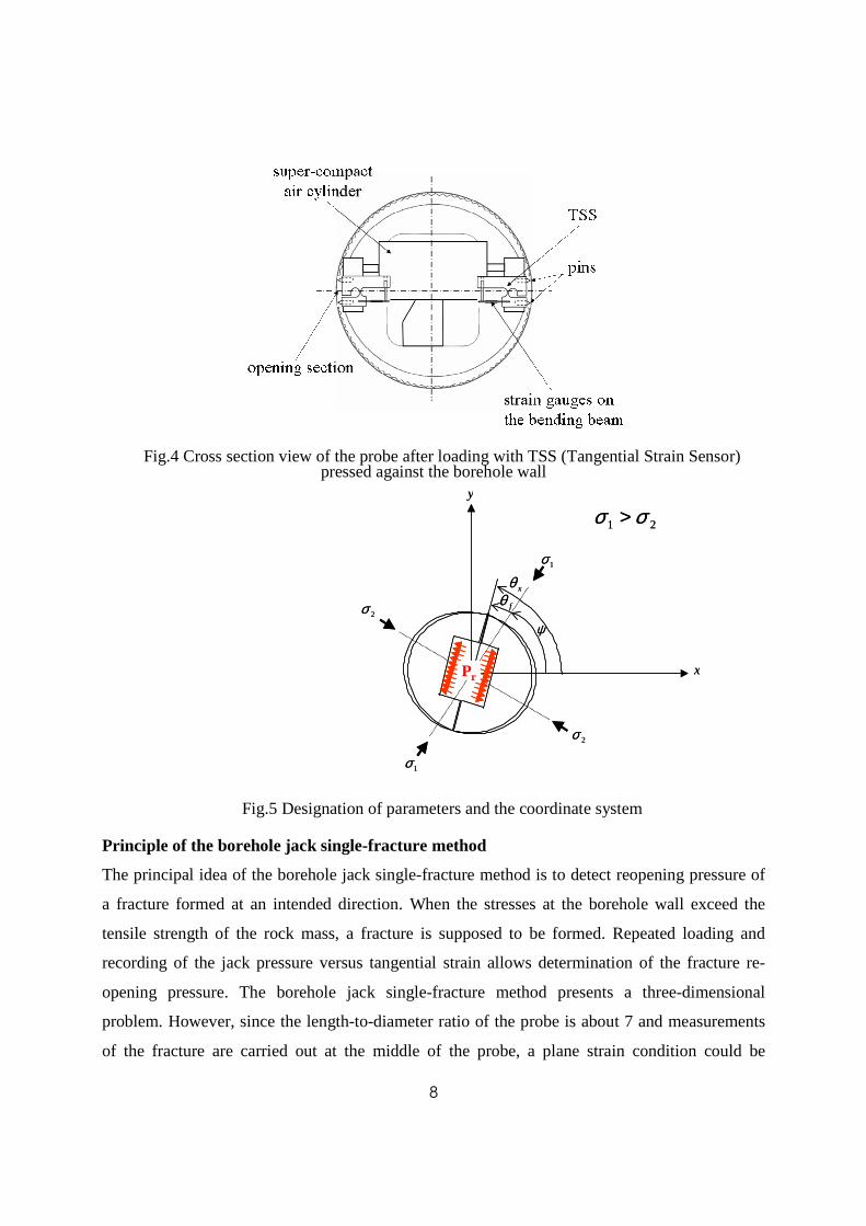
of the opening sections of the borehole. As shown in Fig.4, the movement of the two tangential

strain sensors is controlled by air pressure from a super-compact cylinder. The pins of the strain

sensors will not press against the borehole wall until loading by the probe. The opening

displacement of the fractures is detected as the displacement between the pins and it is measured

by strain gauges on the bending beam.

8

Fig.4 Cross section view of the probe after loading with TSS (Tangential Strain Sensor) pressed against the borehole wall

ψ

fθxθ

1σ

1σ

2σ

2σ

x

y

21 σσ >

Pr

ψ

fθxθ

1σ

1σ

2σ

2σ

x

y

21 σσ >

Pr

Fig.5 Designation of parameters and the coordinate system

Principle of the borehole jack single-fracture method

The principal idea of the borehole jack single-fracture method is to detect reopening pressure of

a fracture formed at an intended direction. When the stresses at the borehole wall exceed the

tensile strength of the rock mass, a fracture is supposed to be formed. Repeated loading and

recording of the jack pressure versus tangential strain allows determination of the fracture re-

opening pressure. The borehole jack single-fracture method presents a three-dimensional

problem. However, since the length-to-diameter ratio of the probe is about 7 and measurements

of the fracture are carried out at the middle of the probe, a plane strain condition could be

9

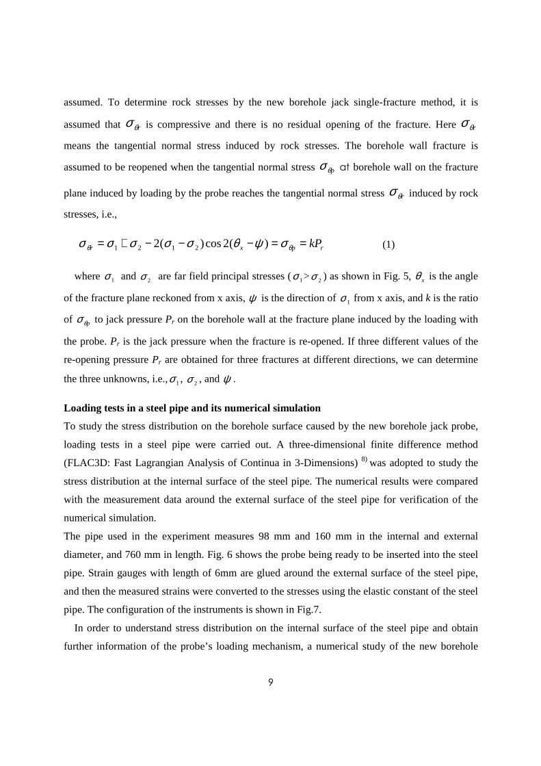
assumed. To determine rock stresses by the new borehole jack single-fracture method, it is

assumed that rθσ is compressive and there is no residual opening of the fracture. Here rθσ

means the tangential normal stress induced by rock stresses. The borehole wall fracture is

assumed to be reopened when the tangential normal stress pθσ at borehole wall on the fracture

plane induced by loading by the probe reaches the tangential normal stress rθσ induced by rock

stresses, i.e.,

rpxr kP==−−−+= θθ σψθσσσσσ )(2cos)(2 2121 (1)

where 1σ and 2σ are far field principal stresses (1σ > 2σ ) as shown in Fig. 5, xθ is the angle

of the fracture plane reckoned from x axis, ψ is the direction of 1σ from x axis, and k is the ratio

of pθσ to jack pressure Pr on the borehole wall at the fracture plane induced by the loading with

the probe. Pr is the jack pressure when the fracture is re-opened. If three different values of the

re-opening pressure Pr are obtained for three fractures at different directions, we can determine

the three unknowns, i.e.,1σ , 2σ , and ψ .

Loading tests in a steel pipe and its numerical simulation

To study the stress distribution on the borehole surface caused by the new borehole jack probe,

loading tests in a steel pipe were carried out. A three-dimensional finite difference method

(FLAC3D: Fast Lagrangian Analysis of Continua in 3-Dimensions) 8) was adopted to study the

stress distribution at the internal surface of the steel pipe. The numerical results were compared

with the measurement data around the external surface of the steel pipe for verification of the

numerical simulation.

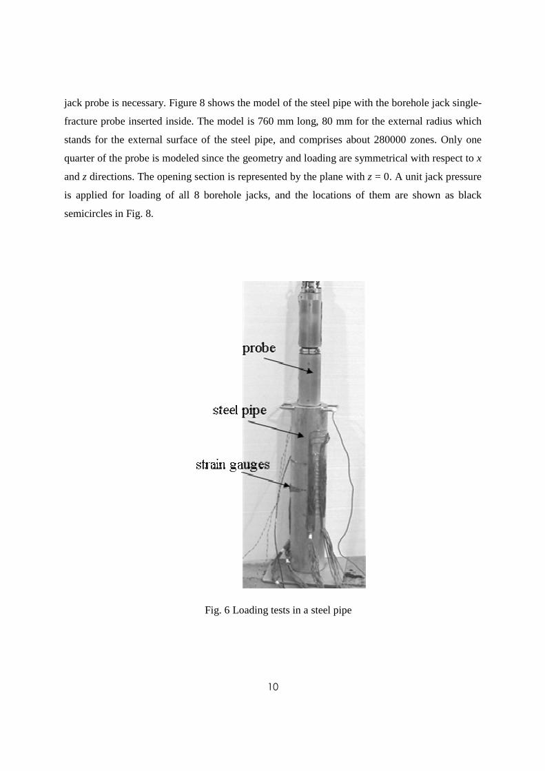
The pipe used in the experiment measures 98 mm and 160 mm in the internal and external

diameter, and 760 mm in length. Fig. 6 shows the probe being ready to be inserted into the steel

pipe. Strain gauges with length of 6mm are glued around the external surface of the steel pipe,

and then the measured strains were converted to the stresses using the elastic constant of the steel

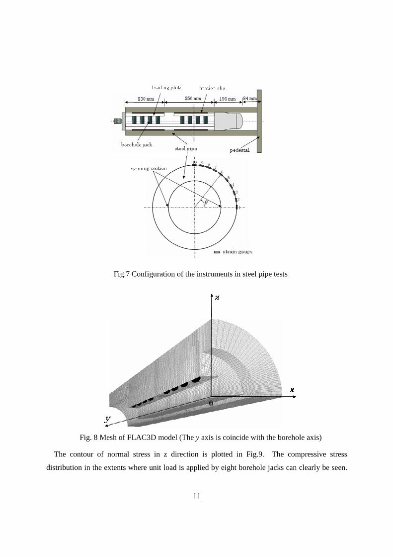
pipe. The configuration of the instruments is shown in Fig.7.

In order to understand stress distribution on the internal surface of the steel pipe and obtain

further information of the probe’s loading mechanism, a numerical study of the new borehole

10

jack probe is necessary. Figure 8 shows the model of the steel pipe with the borehole jack single-

fracture probe inserted inside. The model is 760 mm long, 80 mm for the external radius which

stands for the external surface of the steel pipe, and comprises about 280000 zones. Only one

quarter of the probe is modeled since the geometry and loading are symmetrical with respect to x

and z directions. The opening section is represented by the plane with z = 0. A unit jack pressure

is applied for loading of all 8 borehole jacks, and the locations of them are shown as black

semicircles in Fig. 8.

Fig. 6 Loading tests in a steel pipe

11

Fig.7 Configuration of the instruments in steel pipe tests

Fig. 8 Mesh of FLAC3D model (The y axis is coincide with the borehole axis)

The contour of normal stress in z direction is plotted in Fig.9. The compressive stress

distribution in the extents where unit load is applied by eight borehole jacks can clearly be seen.

12

The stresses reach the maximum tensile stress at the opening section with a uniform distribution

along the axis.

Fig. 9 Contour of normal stress in Z direction under unit jack pressure

To verify the accuracy of the numerical simulation, the simulation results of tangential stresses

along the external surface of the steel pipe are compared with the measured data. In Figure 10,

we can see that the two results agree fairly well. For the numerical results, more samplings are

taken close to the opening section, i.e., from 0 degree to 8 degree, to provide a more accurate

representation of high stress gradient at the external surface of the steel pipe.

-0.8

-0.4

0

0.4

0.8

1.2

0 30 60 90

angle　θ（o）

measured

numerical

-σθ /

Pi

Fig. 10 Comparison between the measured and the numerical stress distributions at the external surface of the steel pipe; jack pressure Pi is compression (negative)

13

The tangential stress distribution at the internal surface of the steel pipe at the middle of the

upper friction shell is shown in Fig. 11. The horizontal axis means the angle measured

counterclockwise from the opening section at the internal surface of the steel pipe. As expected,

the tangential stress reaches the maximum tensile stress at the opening section and then it

decreases smoothly. The tangential stress changes from tensile stress to compressive stress at the

angle of 56 degree from the opening section, and the magnitude of the compressive stress

increases along with the angle. Based on this analysis, the stress concentration factor k shown in

Equation (1) is considered 0.92 for loading in the steel pipe.

-2

-1.5

-1

-0.5

0

0.5

1

1.5

0 30 60 90

-σθ /

Pi

angle θ ( o )

Fig.11 Tangential stress distribution at the internal surface of the steel pipe by numerical simulation

The distribution of the tangential stress at the internal surface is critical for generating and

reopening of fractures at intended directions. All previous jack fracturing techniques had to

consider the influence of a load platen half-contact angle, i.e., an extent where the load platen

contact with the borehole wall, on the stress distribution and fractures were generated either at

the edge of the bearing plates or at the middle of the opening section 9, 10). From Fig.11, however,

we can understand that the tensile stress concentration is generated significantly only at the

opening section as expected. Furthermore, the tangential stress becomes compressive about 60

degrees away from the opening section, which means that the probe can be applied to measure in

situ stress even at the location where there are existing fractures, as long as these fractures are

located along the longitudinal direction in the compressive section by loading of the probe 11).

Chapter Three: Development of a Three-Dimensional BEM for

Inhomogeneous Modeling and Its Application to Rock Slope Stability 12)

14

BEM for inhomogeneous modeling and its algorithm

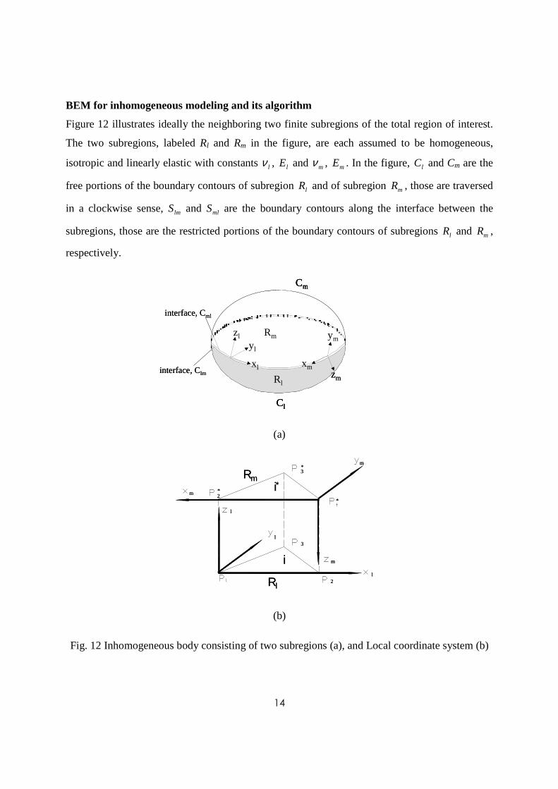
Figure 12 illustrates ideally the neighboring two finite subregions of the total region of interest.

The two subregions, labeled Rl and Rm in the figure, are each assumed to be homogeneous,

isotropic and linearly elastic with constants lν , lE and mν , mE . In the figure, lC and Cm are the

free portions of the boundary contours of subregion lR and of subregion mR , those are traversed

in a clockwise sense, lmS and mlS are the boundary contours along the interface between the

subregions, those are the restricted portions of the boundary contours of subregions lR and mR ,

respectively.

Rl

Rm

Cl

Cm

interface, Cml

interface, Clmxl

yl

zl

xm

ym

zmRl

Rm

Cl

Cm

Rl

Rm

Cl

Cm

interface, Cml

interface, Clmxl

yl

zl

xm

ym

zm

(a)

2

2

3

3Rm

Rl

i

i*m *

*

*

m

m

l

l

l

2

2

3

3Rm

Rl

i

i*m *

*

*

m

m

l

l

l

(b)

Fig. 12 Inhomogeneous body consisting of two subregions (a), and Local coordinate system (b)

15

A boundary value problem for the inhomogeneous body of Figure 12 is defined by the

displacement and stress conditions, which already have been supplied, along the free portions of

the boundary contours lC and mC , as well as by continuity conditions for the displacement and

tractions along the interface between the subregions. The continuity conditions for a point Q of

the interface can be written as

)(~1,

)()(

)()(

)()(

][][

][][

][][

mlMml

QQ

QQ

QQ

ml

ml

ml

Rzx

Rzx

Ryz

Ryz

Rz

Rz

<=

=

−=

=

ττ

ττσσ

(2)

for the stresses, and

)(~1,

)()(

)()(

)()(

][][

][][

][][

mlMml

QuQu

QuQu

QuQu

ml

ml

ml

Rx

Rx

Ry

Ry

Rz

Rz

<=

−=

=

−=

(3)

for the displacement, where M is the number of regions having different elastic constants.

The boundary contours lC , mC , lmC and mlC are divided into a number of triangle leaf

elements, assuming that the displacements and stresses are constant over each element.

Including the portions of the contours that represent the interface, there will be lN boundary

elements along )~1( MlCl = . Then, total number of the elements, N is given by

∑=

=M

llNN

1

(4)

Elements along the two side of the interface must match exactly. There will be then six

unknowns associated with each interface element along each interfaces between two subregions

lR and mR : three displacement components zU , yU and xU , and three traction components

yz σσ , and xσ . Continuity Conditions (2) and (3) give six relations to be satisfied at each

interface element, and so the problem is soluble.

16

Examination of applicability

Boundary contours of concentric double cylindrical surfaces are considered. It is supposed that

the inner boundary contour with radius a is the free surface boundary subject to the uniform

pressure, -p (Analysis case 1 shown below) and the outer boundary contour with radius b is the

interface between the subregions 1R and 2R (Analysis case 3 shown below). Figure 13 illustrates

the cross section at longitudinal center of the cylindrical contours. This section may be under

plane strain state if the length of outer cylinder is greater than 2.5 times of the diameter of it 6)

and the analytical solution is given as follows:

[ ][ ]

brrbprbp

brarapppbpa

ba

rapppbpaba

rr

rr

≥

′+=′−=

≤≤

′−+′−−

=

′−−′−−

=

22

22

222222

222222

)()(1

1

)()(1

1

θθ

θθ

σσ

σ

σ

(5)

p′ in the above equation is represented by

)1)(1()1(2

)1(222

21

22

baGG

bpap

−−+−−=′

１

１

νν

(6)

where 1ν and 1G are Poisson’s ratio and shear modulus of the subregion 1R and 2ν and 2G are

whose of the subregion 2R .

px

y

a

b

ν1 E1

ν2 E2 θ

Fig.13 Axi-symmetric two subregion model

17

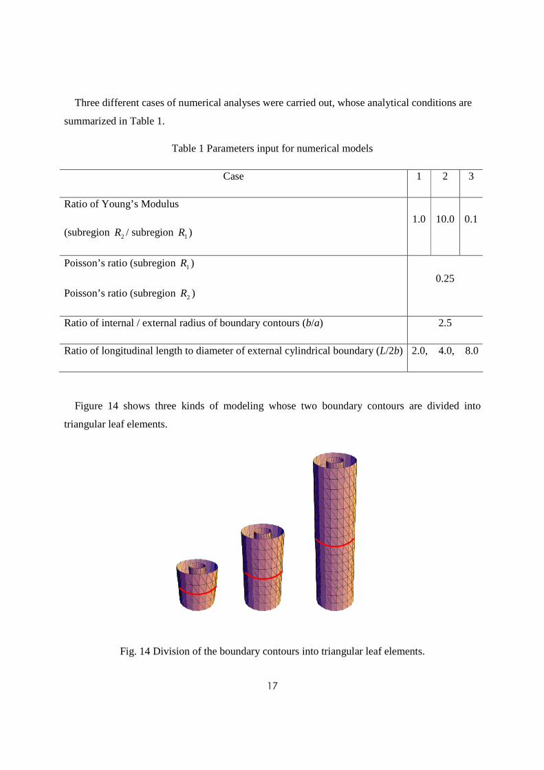
Three different cases of numerical analyses were carried out, whose analytical conditions are

summarized in Table 1.

Table 1 Parameters input for numerical models

Case 1 2 3

Ratio of Young’s Modulus

(subregion 2R / subregion 1R ) 1.0 10.0 0.1

Poisson’s ratio (subregion 1R )

Poisson’s ratio (subregion 2R ) 0.25

Ratio of internal / external radius of boundary contours (b/a) 2.5

Ratio of longitudinal length to diameter of external cylindrical boundary (L/2b) 2.0, 4.0, 8.0

Figure 14 shows three kinds of modeling whose two boundary contours are divided into

triangular leaf elements.

Fig. 14 Division of the boundary contours into triangular leaf elements.

18

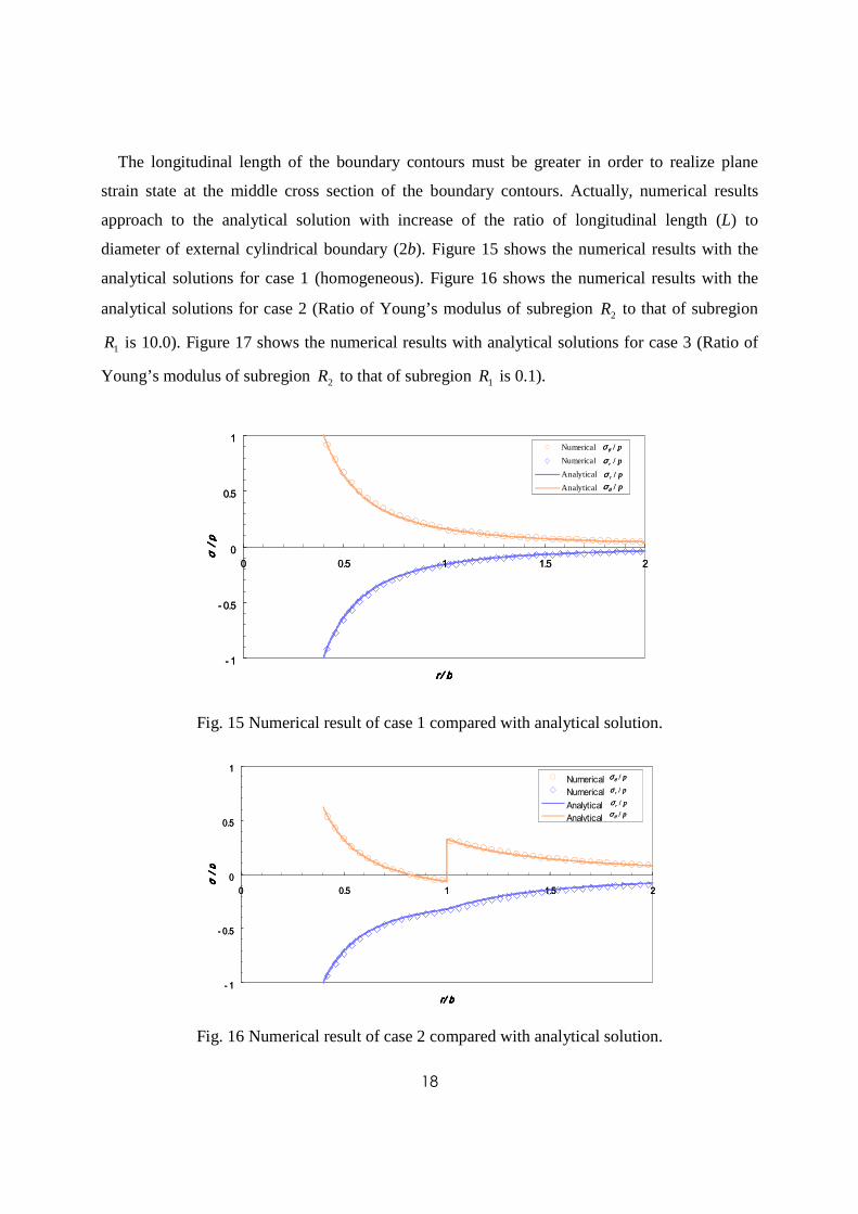
The longitudinal length of the boundary contours must be greater in order to realize plane

strain state at the middle cross section of the boundary contours. Actually, numerical results

approach to the analytical solution with increase of the ratio of longitudinal length (L) to

diameter of external cylindrical boundary (2b). Figure 15 shows the numerical results with the

analytical solutions for case 1 (homogeneous). Figure 16 shows the numerical results with the

analytical solutions for case 2 (Ratio of Young’s modulus of subregion 2R to that of subregion

1R is 10.0). Figure 17 shows the numerical results with analytical solutions for case 3 (Ratio of

Young’s modulus of subregion 2R to that of subregion 1R is 0.1).

- 1

- 0.5

0

0.5

1

0 0.5 1 1.5 2

r / br / br / br / b

σ/p

σ/p

σ/p

σ/p

Numerical

Numerical

Analytical

Analytical

p/θσ

pr /σpr /σp/θσ

- 1

- 0.5

0

0.5

1

0 0.5 1 1.5 2

r / br / br / br / b

σ/p

σ/p

σ/p

σ/p

Numerical

Numerical

Analytical

Analytical

p/θσ

pr /σpr /σp/θσ

p/θσ

pr /σpr /σp/θσ

Fig. 15 Numerical result of case 1 compared with analytical solution.

- 1

- 0.5

0

0.5

1

0 0.5 1 1.5 2

r/ br/ br/ br/ b

σ/p

σ/p

σ/p

σ/p

Numerical Numerical Analytical Analytical

p/θσpr /σpr /σp/θσ

- 1

- 0.5

0

0.5

1

0 0.5 1 1.5 2

r/ br/ br/ br/ b

σ/p

σ/p

σ/p

σ/p

Numerical Numerical Analytical Analytical

p/θσpr /σpr /σp/θσ

p/θσpr /σpr /σp/θσ

Fig. 16 Numerical result of case 2 compared with analytical solution.

19

- 1

- 0.5

0

0.5

1

0 0.5 1 1.5 2

r / br / br / br / b

σ/

pσ

/p

σ/

pσ

/p

Num er ic al

Num er ic al

A naly t ic a l　

A naly t ic a l

p/θσpr /σpr /σp/θσ

- 1

- 0.5

0

0.5

1

0 0.5 1 1.5 2

r / br / br / br / b

σ/

pσ

/p

σ/

pσ

/p

Num er ic al

Num er ic al

A naly t ic a l　

A naly t ic a l

p/θσpr /σpr /σp/θσ

Fig. 17 Numerical result of case 3 compared with analytical solution.

It can be seen that the numerical results coincide enough with the analytical solutions for all

three cases.

Application to rock slope stability evaluation

A limestone deposit of Mount Bukoh exists only in the north side of the mountain and a large

rock slope will be formed with process of mining and one hundred years after, the huge slope

whose size will be 900m high and 5km wide. Therefore slope stability analyses by using three

dimensional boundary element methods have been carried out. Figure 18 shows a landscape view

of Bukoh Mine.

Fig.18 Landscape view of Bukoh Mine.

20

Figure 19 shows the three stages of topographical variation with mining progress along a

vertical section, i.e. (a) the model at the beginning of APS measurement, (b) the model in the

year of 2000 and (c) the model in the future as planned. The boundary between limestone and

schalstein is modeled in the underground as the interface contour as shown in Figure 20.

4 0 0

6 0 0

8 0 0

10 0 0

12 0 0

14 0 0

0 2 00 4 0 0 6 0 0 8 0 0 1 00 0 1 2 00 1 4 00 1 6 00 1 8 00

Schalstein Limestone

Interface

Beginning of APS (1994) In the year of 2000 (1050 mL)Future as planned (2005)

( m )

Ele

vatio

n (m

)

Free boundary

4 0 0

6 0 0

8 0 0

10 0 0

12 0 0

14 0 0

0 2 00 4 0 0 6 0 0 8 0 0 1 00 0 1 2 00 1 4 00 1 6 00 1 8 00

Schalstein Limestone

Interface

Beginning of APS (1994) In the year of 2000 (1050 mL)Future as planned (2005)

( m )

Ele

vatio

n (m

)

Free boundary

Fig. 19 The vertical sections illustrated for three mining stages.

Interface elements

FSM elements

Fig. 20 BEM Model (2000) where the interface is disclosed.

21

Table 2 shows the material properties input for numerical modeling.

Table 2 Material properties input for numerical modeling.

Materials Limestones Schalstein

Young’s modulus E [GPa] 4.12 1.76

Poisson’s ratio ν 0.253 0.249

Density ρ [g/cm3] 2.69 2.94

In numerical modeling, it is assumed that far field stress state may follow the condition of

stress state proposed by Cornet and Vallette 13), which varies linearly with depth (h) as given

follows:

ghkSh ρσ +=)( (7)

=

zyzzx

yzyxy

zxxyx

h

στττστττσ

σ )( ,

=000

0

0

yxy

xyx

SS

SS

S

=100

0

0

yxy

xyx

kk

kk

k , Hzh −=

where g is gravity acceleration and H is the altitude of the highest point of the model. In the

above expression, one of the principal stress direction is assumed vertical and no lateral

heterogeneity is considered. Furthermore, xk and yk is assumed to be )1/( νν − .

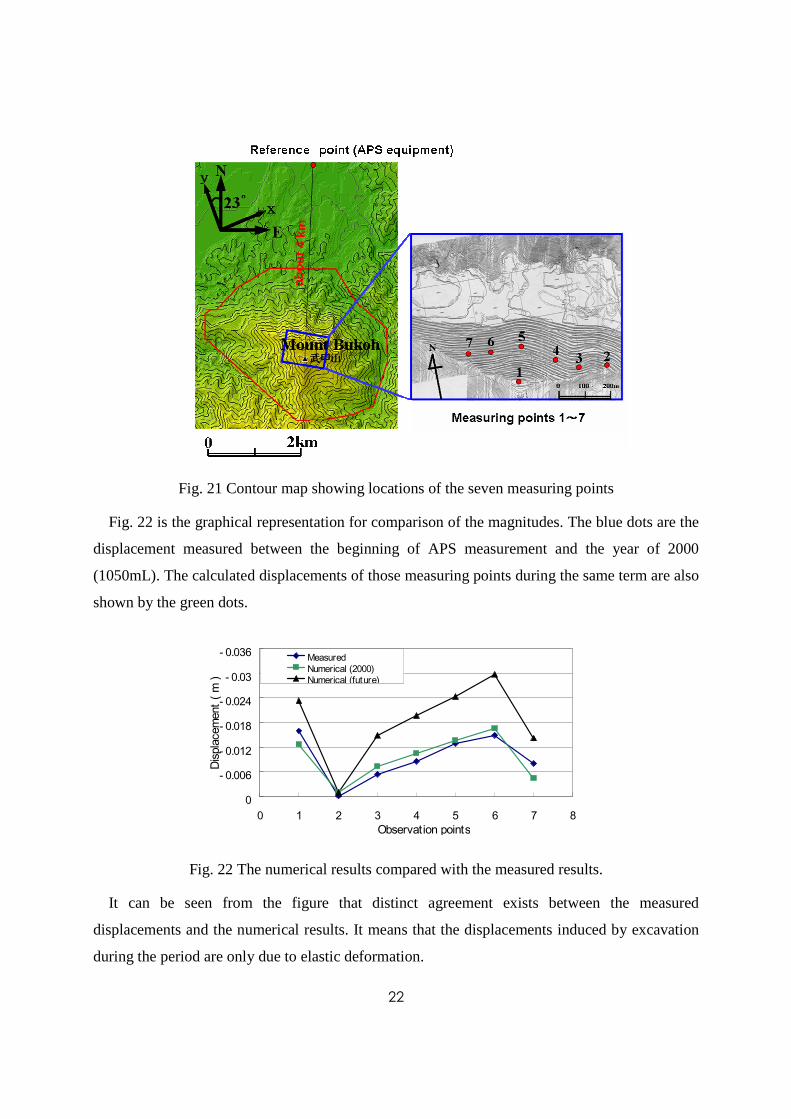
Optical Displacement measurement by APS (Automated Polar System) has been carried out

continuously since November 1994. Figure 21 shows the locations of the seven measuring points

on the surface of man-made rock slope, on the contour map. The reference point where

measuring has been carried out is located about 4km distant in the south direction and thus, the

reference point is greatly below the map.

22

Fig. 21 Contour map showing locations of the seven measuring points

Fig. 22 is the graphical representation for comparison of the magnitudes. The blue dots are the

displacement measured between the beginning of APS measurement and the year of 2000

(1050mL). The calculated displacements of those measuring points during the same term are also

shown by the green dots.

- 0.036

- 0.03

- 0.024

- 0.018

- 0.012

- 0.006

00 1 2 3 4 5 6 7 8

Observation points

Disp

lacem

ent (

m )

MeasuredNumerical (2000)Numerical (future)

Fig. 22 The numerical results compared with the measured results.

It can be seen from the figure that distinct agreement exists between the measured

displacements and the numerical results. It means that the displacements induced by excavation

during the period are only due to elastic deformation.

23

Chapter Four: Stress Field Determination from Local Stress Measurement by

Using Inhomogeneous Three-Dimensional BEM 14)

Overview of methods

The in situ stress field can never be completely measured, and as a result methods for evaluating

stresses involve simplifying assumptions. The assumption of lateral confinement is likely to be

inappropriate in many cases, and factors like tectonic stresses must be considered. The following

equation provides a more general relationship, with the constraints that one of the principal stress

components is vertical and varies linearly with depth:

ghkah

bghSo ραρσ

+++= (8)

where

=

zzo

yyoyxo

xyoxxo

o

σσττσ

σ00

0

0

;

=000

0

0

yyx

xyx

SS

SS

S ;

=

z

y

x

αα

αα

00

00

00

;

=000

0

0

yyx

xyx

kk

kk

k

Here 0σ stands for the in situ measured stress state, S is the tectonic (regional) stress state, α is

the matrix of coefficients due to gravitational loading with the relation that ν

ναα−

==1yx and

1=zα , k is the matrix of coefficients for a linear distribution of horizontal stresses, and a and b

are constants, determined from measured data by a simplex method, that allow for a non-linear

distribution of certain stresses with depth. We emphasize that ,,, xyyx SSS

xyyxzyx kkk ,,,,, ααα are considered as coefficients of far field stress components.

Equation (8) represents a hyperboloid whose asymptotic planes are 0σ = S +α ρ gh and h = -a.

Hence, distribution curves of the stress components in any vertical section are hyperbolas whose

asymptotic lines are σ i0 = Si +αi ρ gh ( i = xx, yy, xy ) and h = -a while σ zz0 =αz ρ gh.

Therefore, σ zz0 is one of the principal stresses.

Thus, for example, the calculated stress component xσ at an arbitrary point i can be expressed

as

xykxyxiykyxixkxxizzxiyyxixxxixysxyxiysyxixsxxixi kkkSSS ,,,,,,,,,c)( σσσασασασσσσσ ααα ++++++++= (9)

24

If the measured stress component xσ at an arbitrary point i is expressed as m)( xiσ , the

following equation is obtained by putting cm )()( xixi σσ = in Equation (9)

zxykxyxiykyxixkxxizzxiyyxixxxixysxyxiysyxixsxxixi kkkSSS ,,,,,,,,,m)( σσσασασασσσσσ ααα ++++++++= (10)

Thus, apply Equation (10) to all stress components at all measurement points, we can obtain

the equation relating all field measurement stress components with the unknown coefficients of

far field stresses.

=

xy

y

x

z

y

x

xy

y

x

kxyxynkyxynkxxynxzxynyxynxxynSxyxynSyxynSxxyn

kxyxykyxykxxyxzxyyxyxxySxyxySyxySxxy

kxyykyykxyxzyyyxySxyySyySxy

kxyxkyxkxxxzxyxxxSxyxSyxSxx

xyn

xy

y

x

k

k

k

S

S

S

ααα

τττττττττ

τττττττττσσσσσσσσσσσσσσσσσσ

τ

τσσ

ααα

ααα

ααα

ααα

,,,,,,,,,

,1,1,1,1,1,1,1,1,1

,1,1,1,1,1,1,1,1,1

,1,1,1,1,1,1,1,1,1

m

1

1

1

MMMMMMMMM

MMMMMMMMM

MMMMMMMMM

MMMMMMMMM

MMMMMMMMM

MMMMMMMMM

M

M

M

M

M

M

(11)

In Equation (11), the parameter n in the last row of the left column stands for the number of

underground measurement points, and the parameter m means that the stresses in the left column

are all field measurement stress components. Since in practice the number of equations is usually

more than 6, i.e., the number of the unknown coefficients xS , yS , xyS , xk , yk and xyk , a unique

solution cannot be guaranteed. A least-squares estimate is adopted here to find the best solution

of the equation.

Calculating elastic gravitational stresses by introduction of a boundary element method for

inhomogeneous bodies

Figure 23 shows a conceptual model showing stress state calculation in a homogeneous linear

elastic region with a topographic surface. Considering principles of linear elastic theory and

continuum mechanics, we assume a horizontal arbitrary plane above the highest elevation of the

surface. Anything under this plane is assumed as one homogeneous linearly elastic body. The

stress state at an arbitrary point under the topographic surface can be calculated by subtracting

25

the induced stress state by the overburden between the horizontal arbitrary plane and the surface,

from the initial stress state under the assumed horizontal arbitrary plane. The initial stress state

under the assumed horizontal arbitrary plane prior to removal of the overburden can be

calculated analytically, corresponding to different far field stress components in Equation (8).

The stresses induced by the overburden from the arbitrary plane to the topographic surface can

be easily solved with the adoption of fictitious stresses in FSM.

Figure 23. Conceptual model showing stress state calculation with a topographic surface

Figure 24. Conceptual model showing stress state calculation for an inhomogeneous body

containing two subregions R1 and R2.

Rock masses are typically heterogeneous and contain discontinuities such as faults. To

adequately estimate the state of stress properly the effects of inhomogeneity must be considered

in certain cases. In Figure 24, we show inhomogeneous rock mass containing two subregions R1

and R2. The two subregions are each assumed to be homogeneous, isotropic and linear elastic.

The common portions of the two subregions define the interface between the subregions. The

lateral extents of the gridded areas must be sufficiently far away from the area of interest such

* *

*

xR2* zR2* yR2*

zR1*

yR1*

xR1*

26

that the behaviour in that area is not greatly affected. The upper subregion can be solved by the

method above for the homogeneous half-plane with a free topographic surface; the lower

subregion with the interface can be treated as the same problem expressed, except that the free

topographic surface is replaced by the interface between the two subregions.

Figure 25. Diagram of Mizunami Underground Research Laboratory (MIU).

500m

500m

82m

27

Application to the stress field determination for underground research laboratory

Mizunami Underground Research Laboratory (MIU), located in Mizunami city of Gifu

Prefecture in central Japan, is under construction for research works 1,000 meter underground

(see Fig. 25). The construction includes two vertical shafts excavated 1,000 m deep underground

and horizontal tunnels at 500 meters level and 1,000 meters level. First stage excavation of the

vertical shafts up to 300m depth has already been carried out. The laboratory shall be utilized as

a base for research of rock mechanics and groundwater flow relating to deep geological

repositories. Local hills reach elevations of 200 meters to 300 meters. Two main geologic units

exist at MIU, a basement of Toki granite and the overlying Akeyo formation of mudstone and

sandstone, which has a maximum thickness of ~150 meters 15). The Tsukiyoshi fault is

recognized east and west on the ground surface in the vicinity of the Shobasama site. It is a

reverse fault with a strike of N80W, a dip of 60 and an estimated throw of about 30m in a gallery

of the Tono Mine.

Rock stress measurements have been performed at 247 points under 9 different locations

within this area by various measurement techniques, including the HF (hydraulic fracturing)

method 15), the DRA (deformation rate analysis) method, and the AE (acoustic emission) method.

The locations of the boreholes for stress measurement are shown from location 1 to location 9 in

Fig. 26, while location 10 stands for the MIU (Mizunami Underground Research Laboratory).

Figure 26. Locations of measurements within the area of simulation. The y-axis points north

and the x-axis points east. Point 10 shows MIU.

28

Sano, Ito, Hirata and Mizuta 16) have reviewed the methods of measuring stress and they have

pointed out the uncertainties in the HF (Hydraulic Fracturing) data interpretation in their article.

It is widely believed without doubt that shut-in pressure, ps, is equal to the minimum principal

stress Sh in the plane perpendicular to borehole axis. In the conventional HF method, the

maximum principal stress is determined through the following equation:

pr = 3Sh – SH – pp (12)

where pr is the reopening pressure, SH is the maximum principal stress and pp is the pore

pressure.

Equation (12) is obtained from the assumption that the fracture closes completely before the

reloading procedure. However, the residual aperture of the induced fracture cannot be negligible

for rocks 17-20). Through numerical simulations, it was suggested that the pressure fluid should

permeate easily into the fracture, even for an initial aperture of 3µ m and the aperture should be

enlarged by the penetration of fluid. Equation (12) should be modified by substituting pr into pp 21,

22) as

2 pr = 3Sh – SH (13)

Regarding this argument, the suggested method presented by the International Society for Rock

Mechanics only notes that “The flow rate should be sufficiently high to prevent fracturing fluid

percolation into the closed fracture before the actual mechanical fracture reopening” 23).

Based on experimental results for a granitic rock mass, Pine et al. 24) considered reopening

pressure as a measure of minimum horizontal stress, namely,

2 pr = Sh (14)

Ito and Hayashi 25) numerically showed that the conventional pr could be equal to ps by

considering that the pressure fluid permeates the fracture deeply before reopening. Rutqvist et al. 26) suggested that the above 3 equations, (12), (13), (14) , might be true for fracture with

extremely small apertures, medium size apertures and sufficiently large apertures, respectively.

In general, numerical simulations in past articles 21, 25, 26) suggest that water permeates at a

lower pressure than conventional reopening pressure, and the conventional pr is affected by flow

rate. Besides, Ito et al. 22) suggest that the conventional pr should also be affected by water

volume in the pressurizing system. When the constant flow rate is so small that the pressure

gradient in the fracture is negligible, temporal variation of pressure are given by them 22), namely

dp/dt = Q/(dVc /dp + C ) (15)

29

where Q, Vc and C are flow rate, volume change due to fracture opening and compliance of the

system, respectively. It is suggested that the conventional pr could only be detected when the

water permeated a fracture several times longer than the borehole radius. This result explained

why the conventional pr is almost equal to ps. They also proposed the use of a high-stiffness HF

system instead of the very compliant conventional HF system.

As it is not easy to make HF system rigid for measurement at deep borehole, the authors used

the conventional HF procedure for local stress measurements described in this paper. However,

in the measurements at the MIU, the flow meter was installed at the position of the straddle

packer and the flow rate at that position was controlled in fracture reopening procedure, while

the flow meter is put at the ground surface in the conventional HF procedure.

First we used BEM method to calculate the matrix of induced state of stresses in Equation (11).

The BEM model for the wide Tono district simulates an area 3.2 km long and 2.4 km wide. The

BEM element size (see Fig. 27) is 200m x 200m in both directions, while the elements that

covers most field-measured locations is finely discretized (100m x 100m) to improve the

accuracy for stress calculation. Introducing of the interface elements simulates two different

kinds of material sub regions including Akeyo formation and the Toki granite. The sub region

between the surface and the interface in Figure 27 stands for Akeyo formation, while the sub

region under the interface stands for Toki granite formation. Tsukiyoshi fault is modelled as

DDM (Displacement Discontinuity Method) joint elements. Elastic constants and densities of the

formations were determined by laboratory tests of core specimens taken from various locations

at various depths.

Taking the tectonic stress component xS as an example, we assumed that xS acts alone on the

BEM model and the induced component of stresses Sxx ,1σ can be achieved by numerical

modelling results of BEM. Second we used a simplex method to determine the two constants a

and b, with a = 904.6 and b = 812.1. A least squares approach is chosen to control the

distribution of error and find the best approximate solution for this over-determined problem 27,

28). Table 3 shows the calculated results for far field stress state.

30

Figure 27. Grid of triangular elements for the BEM modeling. The volume modelled has a plan

view area of 3.2 km x 2.4 km and a depth of 1.2 km. The projection of MIU onto the surface is

shown by a dashed line.

Table 3. Far field stress state determined by BEM3D

Sx (MPa) 1.99

Sy (MPa) 3.45

Sxy (MPa) -0.755

xk 0.778

yk 0.674

xyk -0.168

Fig. 28 summarizes the general magnitudes trends versus depth for the horizontal principal

stresses 1σ and 2σ based on the above BEM-calculated results of the coefficients for the far field

stresses, as well as the vertical stress vσ with a stress gradient of 0.026MPa/m. Here curves of

1σ and 2σ indicate trends that were calculated under the assumption of Equation (8), using the

coefficients determined by the best approximate solution of Equation (11). In most cases the

absolute values of measured horizontal principal stresses, 1σ and 2σ , exceed those of the vertical

31

stresses at shallow depths. The above results show that the stress state measured varied with

depth from thrust fault type (1σ > σ 2 > σ v ) to strike-slip fault type ( 1σ > σ v > σ 2 ).

σv(MPa)

-1200

-1000

-800

-600

-400

-200

0

-60-40-200

measured

calculated

σ2(MPa)

-1200

-1000

-800

-600

-400

-200

0

-60-40-200

measured

calculated

σ1(MPa)

-1200

-1000

-800

-600

-400

-200

0

-60-40-200

measured

calculated

Ele

vatio

n,

m

Figure 28. Summary of the in-situ stresses versus depth for Tono district. The diamonds

indicate the measured stresses.

To illustrate how the above far field stress coefficients can be adopted as input boundary

conditions, FLAC3D is applied to simulate the same area of 3-D BEM analysis. The region

modeled (see Fig. 29) is 3.2 km long, 2.4 km wide and 1.1 km deep. The model was composed

of 280,160 elements and 301,704 gridpoints with an interface to simulate Tsukiyoshi fault. Two

different kinds of material including Akeyo formation and the Toki granite are simulated.

Figure 29. FLAC3D model for Tono district.

32

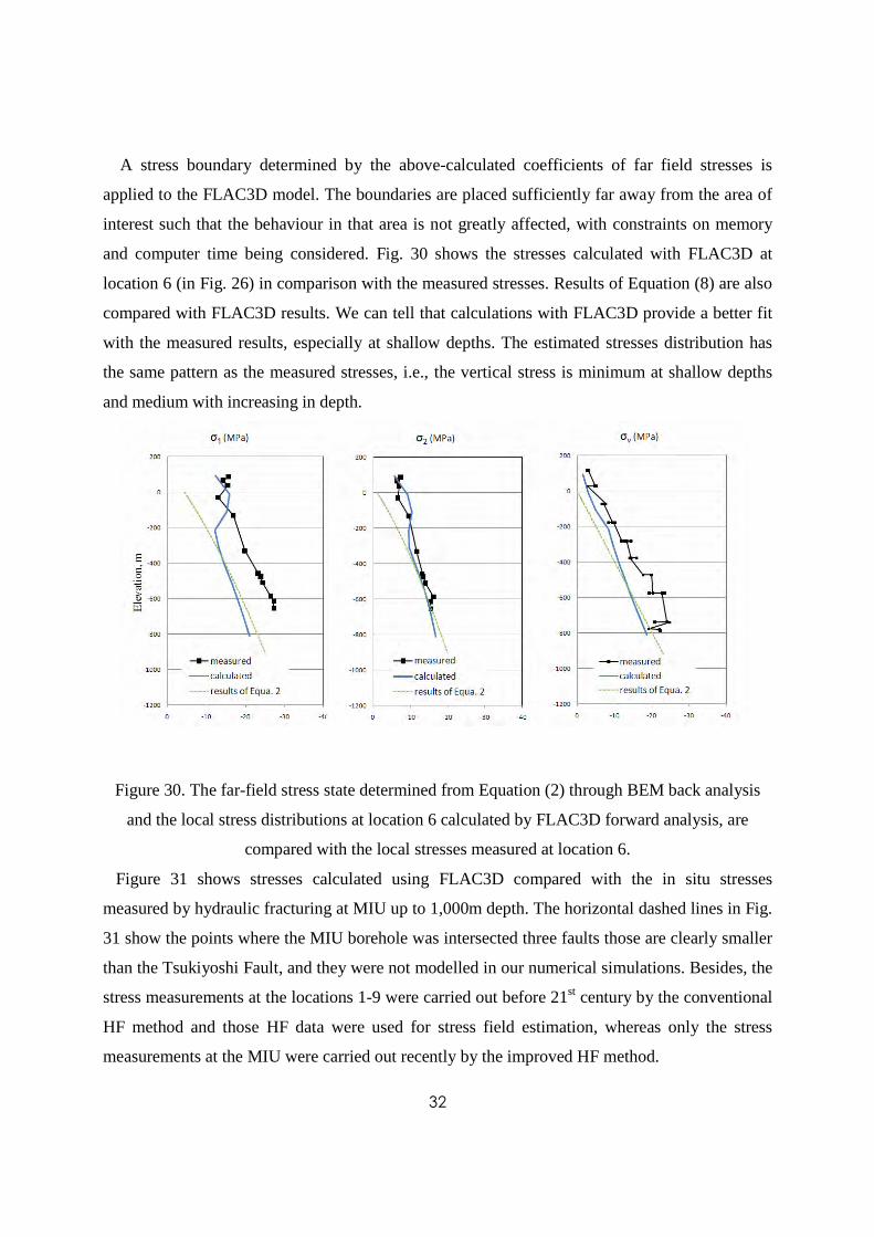
A stress boundary determined by the above-calculated coefficients of far field stresses is

applied to the FLAC3D model. The boundaries are placed sufficiently far away from the area of

interest such that the behaviour in that area is not greatly affected, with constraints on memory

and computer time being considered. Fig. 30 shows the stresses calculated with FLAC3D at

location 6 (in Fig. 26) in comparison with the measured stresses. Results of Equation (8) are also

compared with FLAC3D results. We can tell that calculations with FLAC3D provide a better fit

with the measured results, especially at shallow depths. The estimated stresses distribution has

the same pattern as the measured stresses, i.e., the vertical stress is minimum at shallow depths

and medium with increasing in depth.

Figure 30. The far-field stress state determined from Equation (2) through BEM back analysis

and the local stress distributions at location 6 calculated by FLAC3D forward analysis, are

compared with the local stresses measured at location 6.

Figure 31 shows stresses calculated using FLAC3D compared with the in situ stresses

measured by hydraulic fracturing at MIU up to 1,000m depth. The horizontal dashed lines in Fig.

31 show the points where the MIU borehole was intersected three faults those are clearly smaller

than the Tsukiyoshi Fault, and they were not modelled in our numerical simulations. Besides, the

stress measurements at the locations 1-9 were carried out before 21st century by the conventional

HF method and those HF data were used for stress field estimation, whereas only the stress

measurements at the MIU were carried out recently by the improved HF method.

33

However, when we compare the calculated stresses with the measured ones, good matches can

be found for both the maximum and minimum principal stresses as shown in Fig. 31. Therefore,

the method proposed here provides a practical way to calculate the stress state based on

measured results with reasonable pre-determined boundary conditions by BEM analysis.

Thus, by adopting the stress boundary determined by non-linear far field stress coefficients

calculated from BEM modelling, the in situ state of stress can be determined by FDM simulation

considering tectonic stresses, inhomogeneity and discontinuities of rock mass. With the

understanding of this initial state of stress we can easily study other aspects that we are interested

in along with the excavation of Mizunami Underground Research Laboratory, although more

detailed field formation should be taken into modelling for better estimation of the local stresses.

Figure 31. In situ stresses measured by hydraulic fracturing at depths as great as 1000m at MIU

(location 10 in Fig. 26) compared with the stresses calculated using FLAC3D. The horizontal

dashed lines show the points where the MIU borehole was intersected with the three

discontinuities that are clearly thinner than the Tsukiyoshi Fault.

34

Chapter Five: Concluding Remarks

A study combining strategy and tactics for the determination of in situ rock stress is undertaken

to resolve difficulties and improve accuracy of stress estimation. As a result, a single fracturing

borehole jack probe to improve the applicability and accuracy of deep underground measurement

is developed and the loading test in a steel pipe is carried out for evaluation of the new probe. A

theoretical model considering the tectonic forces, geomorphology and inhomogeneity of rock

masses is proposed, and three-dimensional boundary element method for inhomogeneous

materials has been developed and its applicability has been examined by comparison of the

computed result with strict solution. 3D-FDM forward analysis was carried out for estimation of

the in situ stresses at the specified location after determination of the far-field stress state by 3D-

BEM back analysis.

The following conclusions can be drawn from the above studies:

(1) A new borehole jack single-fracture probe for deep stress measurements is developed. The

new probe includes unique borehole jack loading system and new special tangential strain

sensors to detect the opening of fractures directly.

(2) Loading tests of the new probe in a steel pipe is carried out to study stress distribution on

borehole surface induced by loading with the probe. The measurement data are compared with

the numerical results and they agree fairly well. Through the test and numerical results, it was

found that the probe generates high tensile stress concentration at the opening section where a

fracture is expected to be formed, and the stress concentration factor, k, is 0.92. The tangential

stress turns compressive 60 degrees away from the opening section, which is important for

applying the probe in fractured rock mass since we can ignore effects of preexisting fractures in

this compressive stress region during in situ stress measurement.

(3) The new developed borehole jack single-fracture probe presents the following advantages

over the previous hydraulic or sleeve fracturing techniques. Firstly, a fracture can be generated at

the intended direction based on the unique loading mechanism of the probe. Secondly,

inaccuracies aroused by dealing with fluid pressure distribution in the fracture are not expected

since no fluid is applied to the borehole wall. Thirdly, the opening of the fracture is measured

directly by the tangential strain sensor; therefore the re-opening pressure of the fracture can be

35

detected accurately.

(4) An improved procedure available for inhomogeneous modeling was developed and its

validity was confirmed by comparing the numerical results given by the procedure with the

corresponding strict solution. After that, it was applied to a stability evaluation analysis of man-

made rock slope, and it was confirmed that rock surface displacements at the seven measuring

points to date is due to elastic deformation based on removal of overburden pressure by

excavation progress – because of the agreement between the displacements of the seven points

which were calculated from the models of an inhomogeneous elastic body and the displacements

at the corresponding points, which were actually measured.

(5) A new proposal for the determination of stress distribution based on stress measurement

results considering tectonic stress, topography and inhomogeneity of rock mass is developed in

this paper. The method considered the tectonic stresses, topography and inhomogeneity of the

rock mass. The in situ measurement stress is decomposed into tectonic and gravitational

components, and 6 independent far field stress coefficients are achieved by back analysis using

three-dimensional BEM simulation incorporating inhomogeneity.

(6) To meet the requirement for numerical simulation of the above proposal and solve the

problem concerning boundary assignment, a three-dimensional boundary element method for

determination of gravitational stresses distribution in inhomogeneous rock mass is proposed.

(7) The 3-D BEM and FDM applications to the MIU site have shown that the estimated

stresses agree well with the tendency of the in situ measurement data. It is likely that the tectonic

stresses have to be considered for a better estimation of underground stress distribution in

tectonically active region, such as in Japanese islands. The method described here provides

boundary conditions for commercially available FEM or FDM programs by considering the

influence of tectonic stresses based on stress measurements.

36

Selected References

1) Matsuki K, Kato T, Kimura N, Nakama S, Sato T. Estimation of regional stress for

heterogeneous rock mass by FEM. In: Proc. of the ISRM Int. Symposium 3rd ARMS 2004.

1135-1140.

2) Amadei B, Stephansson O. Rock stress and its measurement. Chapman and Hall; 1997.

p.121-130.

3) Ishida T, Mizuta Y, Nakayama Y. Investigation on a new dry single fracture method of in

situ stress measurement. In. Proc. 3rd Int. Symposium on Rock Stress 2003; 301-306.

4) Crouch SL, Starfield AM. Boundary element methods in solid mechanics. George Allen &

Unwin; 1983. p.47-140.

5) Kuriyama K, Mizuta Y. Three-dimensional elastic analysis by the displacement

discontinuity method with boundary division into triangular leaf element. Int. J. Rock Mech.

Min. Sci. & Geomech. Abstr. 1993; 30:111-123.

6) Kuriyama K, Mizuta Y, Mozumi H, Watanabe T. Three-dimensional elastic analysis by the

boundary element method with analytical integrations over triangular leaf elements. Int. J.

Rock Mech. Min. Sci. & Geomech. Abstr. 1995; 32: 77-83.

7) Liu CL, Mizuta Y, Kuriyama K. Analytical integrations for three-dimensional fictitious

stress method based on Kelvin solution(in Japanese with English abstract), Shigen to Sozai

1999; 115: 719-724.

8) Itasca Consulting Group, Inc. FLAC3D-Fast Lagrangian Analysis of Continua in 3

Dimensions. Version 2.0. User’s Manual. Minneapolis, MN: Itasca. 1997.

9) De la Cruz RV. Jack fracturing technique of stress measurement. Rock Mechanics 1975; 9:

27-42.

10) De la Cruz RV. Modified borehole jack method for elastic property determination in rocks.

Rock Mechanics 1978; 10: 221-239.

11) GANG LI, Y. MIZUTA, T. ISHIDA, O. SANO. Numerical Simulation of Performance

Tests on a New System for Stress Measurement by Jack Fracturing. Journal of the Mining

and Materials Processing Institute of Japan (MMIJ),Vol.121 (2005) No.9, 409-415.

12) C. LIU, GANG LI, K. KURIYAMA, Y. MIZUTA. 'Development of a Computer Program

for Inhomogeneous Modeling by 3D BEM with Analytical Integration and its Application

to Rock Slope Stability Evaluation. Int. J. Rock Mech. Min. Sci, Volume 42 (2005), 137-

37

144.

13) Cornet FH, Valette B. In situ stress determination from hydraulic injection fest data.

Journal of Geophysical Research 1984; 89: 11527-11537.

14) GANG LI, Y. MIZUTA, T. ISHIDA, H. LI, S. Nakama, T. Sato, Stress Field

Determination from Local Stress Measurements by Numerical Modeling. Int. J. Rock Mech.

Min. Sci, (under revision).

15) Nakama S, Sato T, Kato H. Status of study on in-situ stress in the Mizunami Underground

Research Laboratory Project. Proceedings of the 40th U. S. Rock Mechanics Symposium,

Alaska Rocks 2005. CD-ROM 05-887.

16) Sano O, Ito H, Hirata A, Mizuta Y. Review of methods of measuring stress and its

variations. Bull. Earthq. Res. Inst. Univ. Tokyo 2005. 80, p.87-103.

17) Bredehoeft J, Wolff R, Keys W, Shuter E. Hydraulic fracturing to determine the regional in

situ stress field. Piceance Basin Colorado. Geol. Soc. 1976. 87, p.250-258.

18) Zoback MD, Rummel F, Jung R, Raleigh CB. Laboratory hydraulic fracturing experiment

in intact and pre-fractured rock. Int. J. Rock Mech. Min. Sci. & Geomech. Abstr. 1977. 14,

p.49-58.

19) Cornet FH. Analysis of injection tests for in-situ stress determination. Proc. Workshop

hydraulic fracturing stress measurement, Menlo Park. 1982. p.414-443.

20) Durham WB and Bonner BP. Self-propping and fluid flow in slightly offset joints at high

effective pressures. J. Geophys. Res. 1994. 99, p.9391-9399.

21) Hardy MP and Asgian MI. Fracture reopening during hydraulic fracturing stress

determination. Int. J. Rock Mech. Min. Sci. & Geomech. Abstr. 1989. 26, p.489-497.

22) Ito T, Evans K, Kawai K, Hayashi K. Hydraulic fracture reopening pressure and the

estimation of maximum horizontal stress. Int. J. Rock Mech. Min. Sci. & Geomech. Abstr.

1999. 36, p.811-826.

23) Haimson BC, Cornet FH. ISRM suggested methods for rock stress estimation – Part 3:

hydraulic fracturing (HF) and/or hydraulic testing of pre-existing fractures (HTPF). Int. J.

Rock Mech. & Min. Sci. 2003. 40, p.1011-1020.

24) Pine RJ, Ledingham P, Merrifield CM. In situ stress at Rosemanowes Quarry to depths of

2000m. Int. J. Rock Mech. Min. Sci. & Geomech. Abstr. 1983. 20, p.63-72.

25) Ito T, Hayashi K. Analysis of crack reopening behavior for hydrofrac stress measurement.

38

Int. J. Rock Mech. Min. Sci. & Geomech. Abstr. 1993. 30, p.4235-4240.

26) Rutvist J, Tsang CF, Stephansson O. Uncertainty in the maximum principal stress

estimated from hydraulic fracturing measurement due to the presence of the induced

fracture. Int. J. Rock mech. Min. Sci. & Geomech. Abstr. 2000. 37, p.107-120.

27) Mizuta Y. Study on improved procedure for determination of three-dimensional

distributions of the initial rock stresses (Third Report), Japan Nuclear Cycle Development

Institute. 2007. (in Japanese).

28) William M. Geophysical data analysis: Discrete inverse theory. Academic Press, 1989.