1 | E x p - 0

EXPERIMENT 0: MEASUREMENTS, ERRORS AND GRAPHS

0.1. Purpose:

In this experiment, we are interested in learning how to treat data. This is a brief introductory experiment. It aims at teaching the student how to report experimental measurements along with the corresponding errors and the correct number of significant figures. It also aims at familiarizing the student with the manipulation of errors through arithmetic operations, and reporting the correct number of significant figures. Developing the correct method of drawing graphs to represent experimental data is also an aim of this experiment. 0.2. Overview – Theory:

Experimental Errors: Physics is based on measurement. We must learn how to measure the physical quantities in terms of which the laws of physics are stated. Length, time, mass, speed, velocity, acceleration, force, momentum, temperature, charge, voltage, current, resistance ...... are all physical quantities. We use some of these words in our everyday speech very frequently. In physics they have precise meanings, sometimes different than their everyday meanings. In the physics laboratory, and in any other laboratory, we are going to perform experiments. Although the aim of these experiments is very different, they all commonly involve measuring and recording quantities, and deriving from these recorded measurements other quantities which we are interested in determining. We may be measuring the distance between two points on the track of a moving object and the time interval that has passed to go between these points. We may be measuring the electric current flowing through a resistance wire and the voltage across it when the resistance wire is connected across a battery in an electrical circuit. Can a simple quantity like the distance between two points on a track be measured exactly? To measure this distance we use a ruler by laying it along the track and make observations at the two points. We first try to set one of the points at zero on the ruler, but how exactly can we set it at zero? As we know the zero mark on the ruler is usually a line and the line has a certain thickness, which prevents us from getting an exact setting at zero. The same is true for the other point. Reading a value from a ruler involves lining up the two points with the marks on the ruler, and as you can see easily, exact lining up is impossible. The apparent distance between two points, and therefore the values of the reading, depends also on the position of your eye. For example, the position of a point near a ruler may appear different if viewed from the left or right of a line of sight perpendicular to the ruler, as shown in FIG.0-1.

2 | E x p - 0

FIGURE 0-1: Example of parallax in reading the position of a point from a ruler. A reading may appear to be different when viewed with our left eye or right eye, or when we move our head horizontally or vertically over a ruler. This apparent change in position due to a change in the position of the eye is called parallax. There is another possibility that the ruler we use may not be accurate. The size of the ruler may vary with such factors as time, temperature, or humidity. The scale of a measuring instrument is not exact. The exact reading of a scale is impossible. The exact measurement of any quantity is impossible. No experiment gives the right answer. In the physics laboratory the measurements are carried out by means of instruments, such as a ruler, a voltmeter or an ammeter, and whether we like it or not, in all measurements there is always some error (or uncertainty). We aim to get nearer to the right value using more accurate instruments and making our measurements more carefully. Sometimes, we try to make a rough estimate of a quantity and, in such cases, the accuracy of the instrument we use and the way we make our measurement are not very important. In most cases, however, we want to be as accurate as possible. But more than that, we always want to know how accurate our measurements are and how accurate the result which we obtain from our measurements is. When we want to know how accurate a measurement is, we refer to what is called the error in this measurement. The word error does not have the meaning mistake, but rather it is the uncertainty in the measurement as a result of all the contributing factors. As an experimenter, we have to make a reasonable assessment of the accuracy of our measurements detecting the sources of errors and we have to estimate the maximum possible error in each of our measurements. Accuracy expresses how closely the measurement comes to the true or known value. Precision or reproducibility expresses the deviation of a measurement from the average of many measurements using the same procedure repeatedly. Recording Measurements: In recording a measurement, it is important to estimate and record the error. For example, if we measure the distance between two points on a track with a ruler having millimeter division on it, we may record our measurement as

3 | E x p - 0

Distance = 2.5 ± 0.1 cm The significance of ± 0.1 cm is that when we repeat our measurement several more times, the readings we obtain are expected to be one of the values 2.4 cm, 2.5 cm, or 2.6 cm. For many repetitions of the measurement, the value most frequently occurring will be the value 2.5 cm. Note that all readings require both a number and a unit. The error in a measurement can be either positive (reading too much) or negative (reading too little).

How Error in a Measurement is Indicated

We can indicate the error in a measurement in the following two ways: a) We follow the numerical result of our measurement by the symbol ± and then the

maximum possible error, b) We write down the numerical result of our measurement giving only the figures read from

the scale. The last figure given is generally the one in which there is some uncertainty or error.

Look at the following table, which summarizes the experimental values obtained for the speed of light. All the methods used a rotating mirror set up for the measurement. As we see from Table 0-1, no experiment gives the true value of a physical quantity. The experimenter tries to get close to the true value, as Michelson did for the measurement of the speed of light. Notice that he initially could make measurements with an error of ± 50 km/s, finally he could reduce the error down to ± 4 km/s. The accepted value for the speed of light today is 299 792 459.0 ± 0.8 m/s which is in accordance with Michelson's value in 1926, within the estimated limits of error.

Date Experimenter Speed of Light (km/s) 1875 Cornu 299 990 ± 200 1880 Michelson 299 910 ± 50 1883 Newcomb 299 860 ± 30 1883 Michelson 299 850 ± 60 1926 Michelson 299 796 ± 4

TABLE 0-1: Determination of the speed of light using the rotating mirror method

Types of Errors: In general, the types of errors in a particular experiment may be due to the observer, the measuring instrument used, or the experimental design used. All of the possible errors can be considered in two main groups, systematic and random errors.

4 | E x p - 0

Systematic Errors: They are the errors tending to be in one direction only, either positive or negative. They will produce a result, which is always wrong in the same way. If a voltmeter reads 1.2 V when the true voltage is 1.5 V, then there is a systematic error of –0.3 V. The systematic error is not necessarily constant over the entire scale of a measuring instrument. The voltmeter we are considering, when the true voltage is zero, will probably read zero and there is no systematic error. The usual source of systematic errors is the construction or calibration of the measuring instrument. For example, an instrument whose zero setting is wrong gives rise to systematic error and it systematically gives an incorrect reading, either larger or smaller, instead of a true value. We can calibrate an instrument using a standard whose value is known accurately. Systematic errors due to improper calibration, zero setting, etc., can be avoided by proper inspection and adjustment of the instruments and their elimination depends on the skill of the experimenter. In carrying out an experiment it is obviously important to consider possible sources of systematic errors and to take precautions to eliminate them as much as possible. Random Errors: They are the errors tending to be in both directions, negative and positive. These errors are random and produce results, which are both too large or too small. These errors arise from unknown and unpredictable variations in the experimental situation. For example, variation due to parallax or human judgment in interpolating between marks on a ruler used to measure distance between two points produce random error in the result of measurement. They are beyond the control of the experimenter. Inaccurate reading of a scale, unpredictable fluctuations in temperature or line voltage, mechanical vibration of the experimental set up, carelessness in making proper measurement, and other similar accidental reasons can give rise to random errors. They are positive as often as they are negative. We can reduce the effect of random errors by improving the experimental technique, by greater care, by experience and practice, and by improved instruments etc. One way to reduce the random error in a measured quantity is to take the measurement many times and calculate the average of these independent measurements. This will likely be more accurate than a single measurement.

Estimating Errors: Accepting that any measurement is to be in error, it is very important to be able to make good estimates of the maximum possible error or uncertainty in each recorded measurement. The result of a measurement conveys knowledge about a physical quantity and it is a scientific statement. The statement is wrong if it says less or more than is known. The most accurate statement is the one, which says just what is known and no more. When reading a ruler, which is marked in millimeter, we should be able to read to the nearest division. Our maximum reading error should then be ± 1 mm. We may attempt to estimate our reading to less than one division, for example a half or a fifth of a division, by making our reading more carefully. The error in these cases would be ± 0.5 mm or ± 0.2 mm, respectively. Certainly, ± 0.2 mm is an overestimate since with the naked eye a fifth of a

5 | E x p - 0

millimeter division is very difficult to observe. A half of a millimeter, ± 0.5 mm can be observed easily and it is better always to be on the cautious side. For example, a reading from such a ruler might be recorded as 25.5 ± 0.5 mm or 2.55 ± 0.05 cm. Notice that, the last figure shown is the one in which there is some uncertainty.

Significant Figures and Recording Measurements: As mentioned previously, one of the ways of indicating the error in a measurement is by the number of figures recorded. This requires that all the figures recorded (including the last one estimated) are significant. For example, for the distance measured with a ruler marked in millimeters we recorded 2.55 ± 0.05 cm, so this distance would be written with three significant figures, 2.55. If we record our measurement (like 2.55 cm) using only significant figures, the amount of error in the measurement is not specified. The measurements 2.55 ± 0.01 cm, 2.55 ± 0.02 cm or 2.55 ± 0.05 cm would all have three significant figures and would all be recorded as 2.55 cm. In recording measurements, the correct number of significant figures must be used and when possible, the more definite indication ± must be added. When we use the significant figure method to record measurements, we need to develop rules for expressing the number of significant figures in calculated results. Give the figures you read from a scale with only the last figure estimated as a result of measurement. Never put extra figures. The digits including the last one estimated are called significant figures. The number of significant figures has nothing to do with the location of the decimal point. Care should always be taken to distinguish between zeros that are significant and those that are not. Thus, if in measuring the distance with a ruler marked in millimeters, the position of the point appeared to be right opposite the 5 mm division following the 2 cm mark, it would be recorded as 2.50 cm and the zero would be significant. However, if the distance measurement were to be stated in meters, like 0.0250 m, or in micrometers (1 micrometer = l µm = 1 × 10–6 m); like 25500 µm, the zeros other than the one which is to the right of 5 would not be significant and they would be serving only to place the decimal point. The number of significant figures in a measurement is determined as follows: 1. The leftmost nonzero digit is the most significant. 2. If there is no decimal point, the rightmost nonzero digit is the least significant. 3. If there is a decimal point, the rightmost digit is the least significant, even if it is zero. 4. All digits between the least and most significant digits are considered to be significant.

Example 0-1: Some measurements are recorded as: 255 mm; 11.1 cm; 2.04 V; 175000 mA; 0.0125 km; 360 g. How many significant figures do we have in these measurements?

6 | E x p - 0

Solution: We have three significant figures in each of these measurements. A difficulty usually arises if the decimal point is omitted and the rightmost digit is zero. For example, the measurement 3.60 m has three significant figures, but what about if the measurement were recorded as 360 cm? By the rules given above, the result 360 cm has only two significant figures, but the last digit zero is actually significant. Without knowledge that the original measurement of 3.60 m contained three significant figures, however, there is no way to tell whether the zero in 360 cm is significant or not. This problem is resolved by writing the measurements in scientific notation or powers-of 10 notation. Thus, writing 360 cm as 3.60 × 102 cm shows explicitly that the rightmost zero is significant. Scientific notation: Write the result of a measurement as two factors; the first factor contains all the significant figures, having one nonzero digit in front of the decimal point, and the second factor is a power-of-10. Let us write the measurements in Example 5-1 in scientific notation: 255 mm = 2.55 × 102 mm 11.1 cm = 1.11 × 101 cm 2.04 V = 2.04 × 100 V 175 000 mA = 1.75 × 105 mA 0.0125 km = 1.25 × 10–2 km 360 g = 3.60 × 102 g Note that in each case above the first factor gives the number of significant figures existing in the corresponding measurement. Calculation with Significant Figures: The calculations carried out with significant figures usually produce extra figures as a result of calculation. However, reporting more figures would imply greater significance than that given by the measurements and a result can not be made more accurate by a calculation. As we know, the last figure of a measurement is estimated and therefore it is doubtful. We may expect the result of calculation to have also only one doubtful figure. This means that only the first doubtful figure from the left of a result is to be reported. When a doubtful figure is added, subtracted, multiplied or divided by another doubtful (or significant) figure, the resultant figure is also doubtful. To show how doubtful figures are carried through a multiplication operation, the estimated (doubtful) figures are indicated by boldface numbers as in the following example:

7 | E x p - 0

1.231 1.5 (least accurate)

×_______ 6155 1231

+________ 1.8465 ( ≅1.8 )

The first doubtful figure from the left is 8 and therefore the result of this multiplication is rounded off to 1.8. Note that the result has two significant figures, 1 and 8, as the least accurate number 1.5 used in the calculation. Multiplication and Division: In the multiplication or division of numerical measurements, retain in the result only as many figures as the number of significant figures in the least accurate number used in the calculation. To show how significant figures are carried through an addition operation, again indicating the doubtful figure by boldface letters, let’s look at the following example:

44.2146 0.16 120.4

1.122 +___________

165.8966 (≅165.9) Note that, the 4 in the 120.4 is the first doubtful digit from the left and it defines the position of the figure where doubt occurs. The first doubtful figure from the left is 8 and the result of this addition is rounded off to 165.9 since the figure after 8 is 9. The rules of rounding off numbers are given in the following paragraph. Note also that, in addition (or subtraction) we can not use the actual number of significant figures in the numerical measurements, but we pay attention to their positions. Addition and Subtraction: When carrying out addition or subtraction with numerical measurements, do not carry the result beyond the first column (from the left) that contains a doubtful digit. The numerical measurements can be rounded off to the desired number of significant figures before they are used in calculations. A numerical measurement is rounded off according to the following rules: 1. In rounding off, the last figure obtained should be unchanged if the figure to the right of it

is less than 5 (0,1,2,3 or 4). 2. The last figure obtained should be increased by 1 if the figure to the right of it is 5 or

greater (5,6,7,8 or 9). According to these rules the number 23.47 is rounded off to three digits as 23.5 and to two digits as 23. Similarly, the number 23.84 is rounded off to three digits as 23.8 and to two digits as 24.

8 | E x p - 0

Rounding off the numbers, in the first example above, before we make the calculations, we find 1.231 1.2 (rounded off) 1.5 (least accurate) 1.5 ×_______ ×_______ 5755 60 1231 12 +________ +________ 1.8065 ( ≅1.8 ) 1.80 (≅1.8) Similarly, in the second example above, we find 44.2146 44.2 0.16 0.2 120.4 120.4 1.122 1.1 +________ +________ 165.8966 ( ≅165.9 ) 165.9 As seen from the results, rounding off the number(s) before the calculation or rounding off the result at the end yields the same value.

Example 0-2: A student measures three quantities, in appropriate units, and records them using the method of significant figures as: A =12.50; B = 2.72; C =1.4. a) How many significant figures are there in these measurements? b) Write these measurements in scientific notion. c) Round off A and B to two significant figures. d) What is the result of multiplying A x C? e) What is the sum of the measurements?

Solution: a) A =12.50; four significant figures. B = 2.72; three significant figures. C =1.4; two significant figures. b) In scientific notation, we write these measurements A = 1.250 × 101 B = 2.72 × 100 C = 1.4 × 100

9 | E x p - 0

c) Rounding off to two significant figures, we find A =12.50 =13 B = 2.72 = 2.7 d) Multiplying by using boldface numbers for doubtful figures, we obtain 12.50 13 1.4 1.4 ×_______ or ×_______ 5000 52 1250 13 +________ +________ 17.500 ( ≅18 ) 18.2 (≅18) e) Summing the numbers 12.50 12.5 2.72 or 2.7 1.4 1.4 +________ +________ 16.62 ( ≅16.6 ) 16.6

Example 0-3: Consider the scales of two different voltmeters, one of which is finely divided while the other one is coarse as shown in FIG.0-2. They are properly zeroed and calibrated using a standard cell (one whose voltage is known to be accurate) in order to avoid systematic errors. Then, the two voltmeters are connected to the same battery and their scales are shown in FIG.0-2. Read the two scales and record your measurements estimating their errors.

FIGURE 0-2: Two voltmeter scales measuring the same voltage.

0

2

1

4 3 6

5

7

8

– +

COARSE SCALE 1.5 ± 0.1 V

0

1 2

3

4

– +

FINE SCALE 1.55 ± 0.01 V

10 | E x p - 0

Solution: From the coarse scale we read 1.5 V. Figure 1 in this reading is certain, but figure 5 is estimated. Maximum possible reading error for the coarse scale is estimated as ± 0.1 V and the result of this measurement can be recorded as 1.5 ± 0.1 V. This means that the true value is between 1.4 V and 1.6 V. From the fine scale we read 1.55 V. In this reading the last figure 5 is estimated although the first two figures, 1 and 5, are certain. In this case, we can estimate that it is likely to be in between 1.54 V and 1.56, or being on the cautious side, between 1.53 V and 1.57 V. Therefore the maximum possible reading error for this scale might be estimated as ± 0.02 V and the result of this measurement can be recorded as 1.55 ± 0.02 V. Scale reading is not the only source of random error; there are cases where the errors of estimation are larger than the divisions on the scale used. For example, in a lens experiment the exact image position may be difficult to locate by focusing. An image distance measured with a ruler marked in millimeters might be recorded as 21.3 cm because the image obtained on the screen was certainly out of focus at 21.0 cm and also at 21.6 cm. In this case, the image distance must be recorded as 21.3 ± 0.3 cm, although the maximum possible error of the scale is ± 0.1 cm, that is ± 1 mm. In such cases, it is advisable to take a number of readings, record them all, calculate the average and then estimate the maximum error by comparing the average with the maximum values recorded. As explained before, repeating a measurement reduces the magnitude of random errors since they tend to be eliminated.

Example 0- 4: A steel ball is placed at the top of a track, which is mounted on a table as shown in FIG. 0-3. When released, the steel ball rolls down the track and it rolls off the edge of the table. It travels a horizontal distance x, the range, from the edge of the table before it strikes the floor. The experiment is repeated under conditions as identical as possible for each release of the steel ball, but it strikes the floor not exactly at the same point and a spread of impact points is produced. This result is uncontrollable, due to all random effects inherent in the experiment. How can you give a single value as the range of the steel ball?

FIGURE 0-3: The fall of a steel ball released at the top of a track mounted on a table.

x

Track Table

Track Impact points

xmin Table xav

xmax

(Side (Top

Floor

11 | E x p - 0

Solution: If a single value is to be given as the range of the steel ball, it should be the distance from the edge of the table to the center of the distribution of impact points. Under the random effects we expect the distribution of the impact points to be symmetrical about the central point where impact points are the densest. In order to quote a single value as the range of the steel ball, measure the range x for each release, record all of them in a table, calculate the average range xav, and then compare this average with the extreme values recorded to estimate the maximum possible error in the average range. This is shown on the left in Table 0-2 for 10 measurements.

Trial no.

Range x (cm) Deviations d = x – xav (cm)

Deviations squared d2 (cm2)

1 72.4 + 0.7 0.49 2 79.5(max.) + 6.0 36.00 3 73.0 – 0.5 0.25 4 76.6 + 3.1 9.61 5 69.4 – 4.1 16.81 6 67.8(min.) – 5.7 32.49 7 70.6 – 2.9 8.41 8 76.5 + 3.0 9.00 9 75.3 + 1.8 3.24 10 71.9 – 1.6 2.56

TABLE 0-2: The range of a steel ball.

x x x x1 1 2 3∑ = + + +.... d d d∑ = + +1 2 .... d d d d212

22

32

∑ = + + +....

x∑ = ≅734 8. cm 735 cm d∑ = ≅29 4. cm 29 cm d2 118 9 119∑ = ≅. cm cm2 2

xx

av =∑

= =10

735

10735. cm d

dav = = ≅∑

10

29

102 9. cm d

dav2

2

10

119

10119= = =∑ . cm2

σ = = =dav2 119 35. . cm

The size of the spread of impact points can be used to estimate the maximum possible error in the average range. The maximum possible error can be calculated as

Maximum possible error = Spread in x

2 2=

−x xmax min

= − = = ≅79 5 67 8

2

117

2585 59

. . .. . cm

The average range and its maximum possible error can be written as xav=73.5 ± 5.9 cm.

12 | E x p - 0

As explained before, taking the average value of a series of measurements of a quantity will reduce the error since positive and negative random errors tend to cancel each other out. What then is the maximum error of the average value? In this case, we look for the average possible error instead of the maximum possible error in the average. In Table 0-2, the differences between the average and each measurement (or deviations) are tabulated in the third column and the average deviations dav are then calculated. In this calculation, the sign of each deviation is not taken into consideration, since the way the deviation lies makes no difference in the error. The average deviation can be considered as an average possible error and it can be taken as the possible error in the mean value xav. Consequently, the average of the range measurements can be written as 73.5 ± 2.9 cm to indicate that the true value of the range has a high possibility of being between 73.5 – 2.9 = 70.6 cm and 73.5 + 2.9 = 76.4 cm. According to statistical theory, the arithmetic average of a number of observations gives the most probable result and if a very large number of measurements were made, 58% of them would lie inside the interval ± dav. That is, 58% of the impact points of the steel ball would be between 70.6 cm and 76.4 cm from the edge of the table. Let us assume that we measure the range 10 times more and calculate a second average range; this second value would in general differ from the value of the first, but the difference would be expected to be less than the average deviation dav of either set. If we continue like that and make many sets of 10 measurements, we can calculate an overall average of all of the measurements. Then we can calculate the average deviation of the overall mean as we do for a single set of measurements. This procedure is fortunately not necessary, since the statistical theory presents a way of expressing the average deviation of the mean (A.D.) of N measurements. It is calculated as

A DN

. .= Average deviation of N measurements

For the range measurements we have

A Ddav. .

. .

..= = = =

10

2 9

10

2 9

320 9 cm

The significance of the A.D. is that the probability of the true value of the quantity being measured to be within ± A.D. of the mean is 50%. Thus, in the example of the steel ball for 10 measurements, the average range is 73.5 and the average deviation dav from this value is 2.9 cm. This says that, on the average the measurements differ from the average 73.5 cm by ± 2.9

cm. The average deviation of the mean (the A.D.) is 0.9 cm, that is 2 9 10. . This says that the probability of the true value of the range to be in the interval 73.5 ± 0.9 cm is 50%. We use the average deviation of the mean (A.D.) as the best estimate of the error of the measured mean and call it probable error. The probable error is smaller than the maximum possible error and the average error because only an unlikely coincidence will cause every error to reinforce. The maximum possible error, however, is more easily understood and is estimated very easily. The dispersion (scatter of experimental values) is measured in terms of the standard deviation. It is defined as the square root of the average of the squares of the individual deviations from the mean. The symbol of standard deviation is σ and it is calculated by

13 | E x p - 0

σ = =+ + +∑ d

N

d d d

NN

2

12

22 2.......

where d's are the deviations of the measurements from their mean. In the example of the steel ball, the standard deviation σ is also given in Table 5-1. Like the maximum possible error, the average error and the probable error, the standard deviation gives information about the scatter of measurements about the mean. Statistically it is known that for a large number of measurements distributed symmetrically about the mean, about 68% of them will be within ±a. In our results of the steel ball after a large number of measurements we would expect to find about 68% of the impact points with a range of 73.5 ± 3.5 cm. Problem 0-1: A student is going to determine the best reception frequency of a radio receiver for a certain transmitter station. He can read the tuning frequency to the nearest tenth of a division. His readings, in suitable units, are recorded as 15.3; 15.7; 14.8; 16.2; 15.9; 16.1; 15.3; 15.6 a) Arrange these values as in Table 0-2 and calculate the tuning frequency. b) What is the maximum possible error in the tuning frequency? c) What is the average error in the tuning frequency? d) What is the probable error in the tuning frequency? e) What is the standard deviation of the recorded frequencies? Expressing Errors: The error in a measured quantity may be expressed either as the absolute error or the fractional (or relative) error. The absolute error has the same units as the measured quantity. For example, a distance measurement made with a ruler marked in millimeters can be expressed as 25.5 ± 0.5 mm. The absolute error in this quantity is ± 0.5 mm. The fractional error is the ratio of the absolute error to the quantity and it can be expressed as

Fractional error = Absolute error (in the quantity)

Quantity

Note that, the fractional error has no unit and it is commonly expressed as a percentage to give the percentage error of the measured quantity. The percentage error can be expressed as

Percentage error = Fractional error × 100% In the distance measurement given above we have Distance = 25.5 ± 0.5 mm

14 | E x p - 0

Absolute error = 0.5 mm

Fractional error = 0.5

25.5

1

510.02= =

Percentage error = 0.02 × 100 % =2 % A quantity Q is experimentally measured (either as a single reading or as an average of many readings) as x. ∆x is the estimated absolute error in x. The measured value of the quantity Q should be recorded either with its absolute error as Q = x ± ∆x (with the absolute error) or with its percentage error as

Q = x 100%± ×∆x

x(with percentage error)

Example 0-5: The scale in FIG.0-4. is in centimeters. Only the first centimeter is marked in millimeters while the others are left unmarked. a) Estimate the position of arrows A and B by reading the scale. b) Estimate the absolute maximum possible error in these readings. c) Calculate the percentage error in these readings. d) Can you estimate the position of the arrows A and B to 0.01 cm? To 0.001 cm?

FIGURE 0-4. Example 0-5. Solution: a) This example is similar to Example 1-2. When we read the position of arrow A and B we

find the position of arrow A = xA = 0.63 cm the position of arrow B = xB = 2.6 cm

b) Indicating the absolute error in position by ∆x, we obtain

∆xA = 0.01 cm ; ∆xB = 0.1 cm

15 | E x p - 0

c) Indicating the percentage error by P.E., we find

( . .).

..P E

x

xAA= × = × = ≅

∆100%

0 01

063100% 16% 2%

( . .).

..P E

x

xBB= × = × = ≅

∆100%

0 01

2 6100% 3 9% 4%

d) To 0.01 cm; arrow A, yes; arrow B, no; to 0.001 cm; both arrows, no.

Combination of Errors in Calculated Results: Whenever measurements are used in a calculation, an error is associated with the result obtained. The manner in which the error of each measurement propagates and combines depends upon the mathematical calculation used. Suppose we have two measurements x and y with respective errors (maximum possible, probable, average or as standard deviation) ∆x and ∆y. We record our measurements as x ± ∆x and y ± ∆y. The examples that follow discuss the types of calculation we may have with these measurements. Addition and Subtraction: Suppose we add the measurements x ± ∆x and y ± ∆y to find the result R and we want to determine the maximum possible error ∆R in R. The calculated value is R = x + y When the errors ∆x and ∆y happen to reinforce each other, the result R could be as large as R + ∆R = ( x + ∆x ) + ( y + ∆y ) = ( x + y ) + ( ∆x + ∆y ) The result R could be as small as R – ∆R = ( x – ∆x ) + ( y – ∆y ) = ( x + y ) – ( ∆x + ∆y ) So, we can write the result R with its maximum possible error ∆R as R ± ∆R = ( x + y ) ± ( ∆x + ∆y ) Thus the absolute maximum possible error is ∆R = ∆x + ∆y

16 | E x p - 0

When we want to find the difference R = x – y, the difference could be as large as R + ∆R = ( x + ∆x ) – ( y – ∆y) = ( x – y ) + (∆x + ∆y ) The difference R could be as small as R – ∆R = ( x – ∆x ) – ( y + ∆y ) = ( x – y ) – ( ∆x + ∆y ) So we can write for the difference R ± ∆R = ( x – y ) ± ( ∆x + ∆y ) The absolute maximum possible error is ∆R = ∆x + ∆y Note that the maximum possible error in both addition and subtraction is the sum of the individual errors in the quantities. When measured quantities are added or subtracted, the maximum possible error in the result is the sum of the errors in the quantities used in the calculation. When we add two measured quantities x ±∆x and y ±∆y, the sum is (x + y) ± (∆x + ∆y). In writing the sum in this way we assume that the errors ∆x and ∆y are in the same direction to reinforce each other. However, statistically, the probability of the two errors being in the same direction is equal to the probability of the two errors being in the opposite directions. We would like, of course, them to be in opposite directions and therefore they would cancel out each other, but this can not be counted on. In order to be safe, we assume the worst and use the maximum possible error of the result. Statistically, however, the individual errors ∆x and ∆y in the measured quantities are most probably combined in such a way that the probable error in the result is the square root of the sum of the squares of the individual errors. Thus,

The probable error in the result = ( x) ( y)2 2∆ ∆+

For the experiments covered in this manual, the maximum possible error, which is easier to find than the probable error, will mostly be used.

Example 0-6: A student obtained the distances by making measurements such as x ± ∆x = 12.42 ± 0.01 cm y ± ∆y = 8.61 ± 0.01 cm z ± ∆z = 18.36 ± 0.02 cm t ± ∆t = 12.04 ± 0.02 cm

17 | E x p - 0

Calculate the difference D = x – y and the sum S = z + t with their maximum possible errors ∆D and ∆S, respectively. Solution: 12.42 ± 0.01 cm 18.36 ± 0.02 cm 8.61 ± 0.01 cm 12.04 ± 0.02 cm +__________________ +__________________ D ± ∆D = 3.81 ± 0.02 cm S ± ∆S = 30.40 ± 0.04 cm Note that the error in each of the calculated results is the sum of the individual errors in both cases. We can check this by using the values, which will give the greatest and smallest results.

Greatest x = 12.42 + 0.01 Smallest x = 12.41 – 0.01 = 12.43 cm = 12.41 cm Smallest y = 8.61 – 0.01 Greatest y = 8.61 + 0.01 = 8.60 cm = 8.62 cm Greatest D =12.43 – 8.60 Smallest D =12.41– 8.62 = 3.83 cm = 3.79 cm Note that the notation D ± ∆D = 3.81 ± 0.02 cm gives the same result. Check for the sum S following the same steps. Multiplication and Division: Suppose we want to calculate the product P of two measurements x ± ∆x and y ± ∆y. We can write the calculated value as

P = x . y When the errors ∆x and ∆y happen to reinforce each other, the product P could be as large as P P x x y y+ = + +∆ ∆ ∆( ). ( )

= + +

= + +

= + + +

xx

xy

y

y

x yx

x

y

y

x yx

x

y

y

x y

x y

( ). ( )

. ( )( )

. (.

.)

1 1

1 1

1

∆ ∆

∆ ∆

∆ ∆ ∆ ∆

The last term ∆ ∆x y

x y

.

. in the parenthesis can be neglected since both

∆x

x and

∆y

y are small;

hence product ∆ ∆x y

x y

.

. is much smaller. We have

18 | E x p - 0

P P x yx

x

y

y+ = + +∆ ∆ ∆

. ( )1

The product P could be as small as P P x x y y− = − −∆ ∆ ∆( ). ( )

= − −

= − − +

xx

xy

y

y

x yx

x

y

y

x y

x y

( ). ( )

. (.

.)

1 1

1

∆ ∆

∆ ∆ ∆ ∆

Again, neglecting the last term in the parenthesis

P P x yx

x

y

y− = − −∆ ∆ ∆

. ( )1

Therefore the product P and its maximum possible error ∆P can be written as

P P x y x yx

x

y

y± = ± +∆ ∆ ∆

. . ( )

Comparing the two sides of this equation and noting that P = x.y, we can write

∆ ∆ ∆P P

x

x

y

y= +( ) or

∆ ∆ ∆P

P

x

x

y

y= +( )

We see that in the multiplication of two measurements, the maximum relative error ∆P

P

in the product is equal to the sum of the relative errors in the quantities multiplied. In terms of the percentage errors we can write

∆ ∆ ∆P

P

x

x

y

y× × + ×100 = 100 100

Suppose we want to calculate the division D of two measurements x ± ∆x and y ± ∆y. Assume

that we have the division Dx

y= . The division D can be written as

D = x.y–1

Following the same procedure as for the multiplication we can easily show that

∆ ∆ ∆D

D

x

x

y

y× × + ×100 = 100 100

19 | E x p - 0

When measured quantities are multiplied or divided, the maximum percentage error of the result is the sum of the percentage errors in the measured quantities used in the calculation. Powers: The calculation carried out with measured quantity x to obtain the final result R is of the form of

R = xn

in which n is usually an integer. This calculation means that the measured quantity is multiplied n times by itself. That is

R = xn = x.x.x .......... x (n times) Then by applying the result of the multiplication, the maximum error ∆R in the result is given in terms of the percentage errors by

∆ ∆ ∆ ∆R

R

x

x

x

x

x

x× × × ×100 = ( 100)( 100).......( 100)

∆ ∆R

R

x

x× ×100 = n( 100)

The calculation with measured quantities x, y and z to obtain the final result R is in the form of

Rx y

zx y z

n m

k

n m k= = −.. .

In this case, the maximum error ∆R in the result is given in terms of the percentage error as

∆ ∆ ∆ ∆R

R

x

xm

y

yk

z

z× × + × ×100 = n( 100) 100)+ 100)( (

Example 0-7: A student uses a simple pendulum to determine experimentally the acceleration due to gravity. He measures the length l and period T of the pendulum and uses the relation

Tl

g= 2π

from which the acceleration due to gravity is

gl

T= 4 2

2

π

20 | E x p - 0

For the simple pendulum the student uses, the measurements are l ± ∆l = 100 ± 1 cm and T ± ∆T = 2.00 ± 0.05 s Calculate the acceleration due to gravity g and its error ∆g. Solution: The acceleration due to gravity is calculated as

gl

T= = = =4 4 314 100

2 00986 9 86

2

2

2

2

π ( . ) ( )

( . ). cm / s m / s2 2

The maximum error in the calculated result can be found in terms of the percentage errors using the relation

∆ ∆ ∆g

g

l

l

T

T× × ×100 = ( 100).2 100)(

The maximum percentage errors are

∆l

l× × = 100 =

1

100100 1% and

∆T

T× × = 100 =

0.05

2.00100 2 5%.

The maximum percentage error in the calculated result is

∆g

g× 100 = % + 2(2.5%)= 6%1

Therefore we have

∆g

g× × = 100 =

6

100100 6% and ∆g = = =006 986 59 2 59. ( ) . cm / s2

From the measurements, the student obtains the final result for the acceleration due to gravity as g ± ∆g = 986 ± 59 cm/s2 or in the other unit g ± ∆g = 9.86 ± 0.59 m/s2. After rounding off the numerical values properly, the result can also be written as

g ± ∆g = 990 ± 60 cm/s2 or g ± ∆g = 9.9 ± 0.6 m/s2 Note that we keep only the first decimal place where a nonzero error occurs and round off the rest.

21 | E x p - 0

Trigonometric Calculations: Suppose that an angle θ is measured and is used in the calculation R = sinθ The maximum possible error ∆R is ∆ ∆R= + −sin( ) sinθ θ θ

where ∆θ is the error in the angle θ. Example 0-8: An angle is measured as θ ± ∆θ = 30° ± 1°. Calculate R = cos θ and its maximum possible error ∆R. Solution: R = cos θ = cos 30 ° = 0.87 ∆R = cos ( θ + ∆θ ) – cos θ = cos 31° – cos 30° = 0.86 – 0.87 = 0.01 Thus, the result can be written as

R ± ∆R = 0.87 ± 0.01. Problem 0-2: A student tries to find the Young modulus for brass. He uses a brass wire and measures the length l and the diameter D of the wire as

l ± ∆l = 2.50 ± 0.01 m D ± ∆D = 0.36 ± 0.01 mm

He applies a force and the brass wire stretches by x. His measurements for these quantities are

F ± ∆F = 4.00 ± 0.01 N x ± ∆x = 1.00 ± 0.02 mm

The expression for the Young modulus E is

EF

Ax

l

= =Stretching force per unit area of cross section

Extension per unit length

22 | E x p - 0

where A is the cross-sectional area of the brass wire and it is given by

A RD= =π π2 2

2( )

a) Calculate the percentage error in ; i) each of the measured quantities, ii) the cross-sectional area A of the brass wire, iii) quotients F/A and x/l, iv) the calculated value of E for brass. b) How should the student quote the result of his experiment? c) In order to have smaller error in E, which quantities must be measured more accurately? Graphs: In order to see the quantitative relationship between the physical quantities involved in an experiment, we express our measurement of these quantities in tabular form. Although we can make some prediction from this data table, another very useful way of expressing the data is plotting a graph from it. A graph provides a visual picture of the data and from the graph we can deduce the relationship between two related variable physical quantities. In order to plot a graph of two variables, we use rectangular x- and y-axes. The horizontal axis (x-axis or abscissa) is used for the independent variable, like time t. The vertical axis (y-axis or ordinate) is used for the dependent variable, like the height h from the ground of a ball falling freely. The location of a point on the graph is defined by its coordinates x and y. The coordinates of the point are written as an ordered pair (x, y) and they are measured with respect to the intersection of x- and y- axes called the origin (0,0). A graph should be self-explanatory, and therefore it must have: 1. The titles of the graph on the graph paper (usually written like Height h versus Time t or

like Pressure P versus Temperature T ). 2. The student's and, if any, the partner's name and experiment date. 3. Each axis labeled with the quantity plotted and its proper unit. 4. The scaling so that points are distributed as widely as possible over the area of the graph

paper used to plot the graph. 5. Simple scales to make calculations straightforward (whole number of squares represent

whole unit as a scale). 6. The error bars representing the uncertainty in each reading. From our measurements, we should have a set of points (x1, y1), (x2, y2), (x3, y3) etc. Where x1 and y1 are the coordinates of the first point, and so on. When we plot the data points with their error bars, we do not join all the points together by a zigzag. Instead of this, we try to draw a smooth curve or a straight line, which may not pass through some of the data points. Smooth means that the line we draw does not have to pass exactly through each plotted point, but passes the plotted points as a curve of best fit. The graph we draw, however, indicates how the two quantities depend on each other.

23 | E x p - 0

Analysis of a Straight Line Graph: Two linearly related quantities, x and y, have an algebraic equation of the form

y = mx + b where m and b are constants. When the values of such two quantities are plotted, the graph is a straight line. In many experiments, the result of a set of data usually yields a straight-line graph when we plot it. In practice, however, the measured points will be scattered because of the error they contain and we will be required to draw the best straight line passing through the data points. Picking the best straight line is sometimes difficult, but a transparent ruler may be helpful to make trail lines and try to arrange the line so that an equal number of points lie on either side in a random way. The best straight line, however, must pass inside as many error bars as possible. FIG. 0-5. gives an example of a straight-line graph between two physical quantities x and y. Note that for each measured point the positive and negative maximum possible errors are marked with error bars.

FIGURE 0-5: Example of a straight-line graph with error bars. After we draw the graph of y versus x we want to determine the two constants m and b in the algebraic equation. The m in the algebraic equation is called the slope or gradient of the line and it measures the rate at which y changes with x. In order to calculate the slope m, we take two points, (x1, y1) and (x2, y2), being as far apart as possible on the best straight line fitted to the experimental data points. Slope m is expressed as

my

x= ∆

∆

Error bar(±∆y3)

Error bar(±∆x3)

y Best Line

Worst Line

y4 y5

y3

y2

y1

x 0 x4 x5 x3 x2 x1

24 | E x p - 0

where ∆y and ∆x are the changes in y and x, respectively, as we go from point (x1, y1) to point (x2, y2). They are given by

∆y = y2 – y1 and ∆x = x2 – x1 Thus, slope m can be written as

my

x

y y

x x= =

−−

∆∆

2 1

2 1

Note that, the changes ∆y = y2 – y1 and ∆x = x2 – x1 are different from the maximum possible error ∆y and ∆x in the measurement y and x, respectively. The similar symbolism is merely a coincidence. The b in the algebraic equation is called the intercept and it gives the point where the straight line cuts the y-axis, that is, when x = 0, then y = b. The general equation of a straight-line graph passing through the origin (the intercept b=0) is given by y = mx. Such a relation indicates a direct proportion between the two quantities x and y; then the slope m is the constant of proportionality. After plotting the experimental points (x1, y1), (x2, y2) etc. with corresponding error bars ±∆x1, ±∆y1, etc., and drawing the best straight line through these data points, we determine the slope m and the intercept b from this graph. Actually our task is to determine from the graph the slope as m ± ∆m and the intercept as b ± ∆b, where ∆m and ∆b are the maximum possible errors in slope m and in intercept b, respectively. These errors can be easily determined by drawing the worst possible straight line on the graph. We analyze the worst possible line in the same way to obtain the worst possible slope m' and the worst possible intercept b'; and then we get the possible errors ∆m and ∆b as

∆m m m= − ′ and ∆b b b= − ′

The straight-line graph provides the best way of increasing the accuracy of our experiment. Instead of using a single set of two readings to determine a quantity, we always prefer to collect a set of readings to plot a graph, and we use this graph to obtain the quantity more accurately. As an example, consider a simple electrical experiment in which the resistance R of a wire is determined by measuring the current I flowing through and the corresponding potential difference V across the wire. According to Ohm's law (V = RI, the resistance R is related to the measured quantities I and V through the equation

RV

I= =constant

The error in the calculated R can be reduced by taking several readings of I and V, in each case calculating R and then obtaining an average of all values of R. One disadvantage of this method of determining R is that results differing widely from the average have bigger influence on the calculated value. Therefore, one or two bad results can give a large error in the result and cancel out the value of taking a series of readings and determining the average of them.

25 | E x p - 0

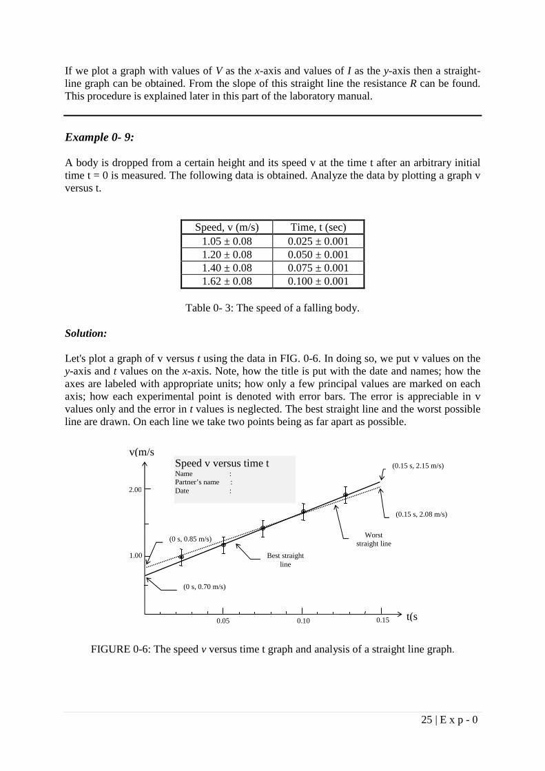
If we plot a graph with values of V as the x-axis and values of I as the y-axis then a straight-line graph can be obtained. From the slope of this straight line the resistance R can be found. This procedure is explained later in this part of the laboratory manual. Example 0- 9: A body is dropped from a certain height and its speed v at the time t after an arbitrary initial time t = 0 is measured. The following data is obtained. Analyze the data by plotting a graph v versus t.

Speed, v (m/s) Time, t (sec) 1.05 ± 0.08 0.025 ± 0.001 1.20 ± 0.08 0.050 ± 0.001 1.40 ± 0.08 0.075 ± 0.001 1.62 ± 0.08 0.100 ± 0.001

Table 0- 3: The speed of a falling body.

Solution: Let's plot a graph of v versus t using the data in FIG. 0-6. In doing so, we put v values on the y-axis and t values on the x-axis. Note, how the title is put with the date and names; how the axes are labeled with appropriate units; how only a few principal values are marked on each axis; how each experimental point is denoted with error bars. The error is appreciable in v values only and the error in t values is neglected. The best straight line and the worst possible line are drawn. On each line we take two points being as far apart as possible.

FIGURE 0-6: The speed v versus time t graph and analysis of a straight line graph.

2.00

1.00

v(m/s

t(s0.15 0.10 0.05

(0 s, 0.70 m/s)

(0 s, 0.85 m/s)

Best straight line

Worst straight line

(0.15 s, 2.08 m/s)

(0.15 s, 2.15 m/s) Speed v versus time t Name : Partner’s name : Date :

26 | E x p - 0

Using the end points of the best straight-line slope, m can be determined. The two end points are (0 s, 0.70 m/s) and (0.15 s, 2.15 m/s) Slope m of the best straight line is given by

my

x

y y

x x= =

−−

= =∆∆

2 1

2 1

9 672.15 m / s - 0.85 m / s

0.15 s - 0 s m / s2.

Similarly, for the worst possible line using the two end points (0 s, 0.85 m/s) and (0.15 s, 2.08 m/s) the slope m' is given by

my

x

y y

x x' .= =

−−

= =∆∆

2 1

2 1

9 672.15 m / s - 0.85 m / s

0.15 s - 0 s m / s2

The maximum possible error in the slope is

∆m m m= − ′ = − =9 67 8 20 147. . . m / s2

The slope of the best straight line with its maximum possible error is

m ± ∆m = 9.67 ± 1.47 m/s2 We can round off the result to the first column in which a nonzero error occurs. Thus we can write the slope as

m ± ∆m = 10 ± 1 m/s2 The intercept b of the best straight line and b' of the worst possible line from the graph are

b = 0.70 m/s b′ = 0.85 m/s

The maximum possible error in the intercept is

∆b b b= − ′ = − =070 085 015. . . m / s The intercept of the best straight line with its maximum possible error is

b ± ∆b = 0.70 ± 0.15 m/s We can round off the result to the first column in which a nonzero error occurs. Thus we can write the intercept as

b ± ∆b = 0.7 ± 0.2 m/s Note that this method is the simplest and easiest way to analyze a straight-line graph. The method of least squares to draw the best straight line through a set of experimental data is out of the scope of this manual.

27 | E x p - 0

One common example of motion with almost constant acceleration is that of an object falling toward the earth from a certain height. When the air resistance is neglected we find that all objects, whatever their size, mass, or composition, fall with the same acceleration, and if the height they fall from is not too great, the acceleration remains constant throughout the motion. Such a motion, in the absence of air friction, is called free fall. The acceleration of a freely falling body is called the acceleration due to gravity and it is directed down toward the center of the earth. It is denoted by the symbol g and near the earth's

surface its magnitude is approximately 9.8 m/s2 (= 980 cm/s2). However, the exact value of it changes with latitude and altitude. The equation relating the speed v and time t (measured from an arbitrary initial time t=0) of an object falling freely down to the ground from a certain height is

v = vo+ gt

where v0 is the initial speed and g is the acceleration due to gravity. Let's write this equation as v = gt +v0 and compare it with the general equation of a straight-line y = mx + n, written in terms of two variables x and y. To do so, let's put the two equations one after another comparing the corresponding terms by the use of arrows in the following fashion;

y = mx + b v = gt + v0

As seen from the correspondence between the two equations, the equation v = gt +v0 is a straight-line equation. From the graphical analysis of v versus t graph we have slope m being equal to acceleration g due to gravity and intercept b to the initial speed v0. From our graphical analysis of the experimental data, we obtain the physical quantities g and v0 as

g ± ∆g = 10 ± 1 m/s2 and v0 ± ∆v0 = 0.7 ± 0.2 m/s Nonlinear Graphs: The following are some non-linear relations in physics: Inverse Proportion: A graph of pressure P versus volume V (FIG. 0-7a) for an ideal gas at constant temperature yields the relationship

PV = k

28 | E x p - 0

where k is a constant. Note that, a graph of P versus 1

V (FIG. 0-7b) would be a straight line

through the origin since the relationship P = k (1

V) is equivalent to the general equation of a

straight-line graph passing through the origin.

FIGURE 0-7: (a) P versus V and (b) P versus 1 / V graphs of an ideal gas at a constant temperature.

A Square Law Graph: A graph of the position x vs. time t (FIG. 0-8a) for an object starting from the origin (x= 0) at rest and moving in the x-axis with constant acceleration can be shown by the following equation

x at= 1

22

Note that, the position x is related non-linearly to the time t. Note also that, a graph of x versus

t2 would be a straight line whose slope would be 1

2a as shown in FIG. 0-8b and it would pass

through the origin.

FIGURE 0-8: (a) x versus t and (b) x versus t2 graphs of an object moving along the x-axis with constant acceleration. The object is initially at rest at the origin.

P1

V2 V1

P1V2 = P2V1 = k

P2

P

V

Slope = k

P

(1/V)

(a) (b)

Slope = (1/2) a

x

t2

x

t

(a) (b)

29 | E x p - 0

An Inverse Square Law Graph: A graph (FIG. 0-9) of force F between the earth and a satellite at different radial distances r

from the center of the earth can be shown by F kr

= 12

where k is a constant. The force F is

depending nonlinearly on the distance r, but it is depending linearly on 12r

.

FIGURE 0-9: Force of attraction F between the earth and a satellite at different radial distances r from the center of the earth.

Exponential Relation: A graph (FIG. 0-10a) of current i flowing through a circuit containing a battery, a resistance R and an initially empty capacitance C in series has an equation given by

i i etRC= −

0 where i0 is the initial (t = 0) current in the circuit, t is the time, e is the base of natural logarithm and equal to 2.718. Taking the natural logarithm of both sides of the equation gives

ln lni it

RC= −0

or

ln ( ) lniRC

t i= − +10

and this equation gives a straight line as in FIG. 0-10b when ln i is plotted as a function of

time t. The slope of this line is − 1

RC and the intercept is ln io.

F

r

30 | E x p - 0

FIGURE 0-10: An initially empty capacitor connected in series with a resistor to a battery; (a) i versus t graph, and (b) ln i versus t graph.

Instead of using natural logarithms to the base 2.718, we can use logarithms to the base 10 and we can plot log i versus t. This graph also yields a straight line and so will the plot of ln i versus t, but with a different slope, because the logarithm of any number to one base is proportional to the logarithm to another base. If we suspect an exponential relationship for a graph plotted between two physical quantities, we try to plot the logarithm of one variable as a function of the other variable. If the relationship is exponential, we obtain a straight line. Such graphs are called semi-log since they are done on graph paper, which is scaled logarithmically along one axis and linearly along the other axis. A logarithmic scale helps us since we can plot without looking up the logarithms of one variable in a table of logarithms. Power Laws: Two variables x and y related by the general equation

y=kxn where k and n are constants, positive or negative. If we take the logarithm of both sides of the equation, we get

log y = log k + n log x or

log y = n log x + log k When we plot log y as a function of log x we obtain a straight line. The slope of this straight line is n and the intercept is log k. We use graph paper that is scaled logarithmically along both axes known as log-log paper and in this way, we do not need to look up the logarithm of either variable.

ln i0

t

Slope = -(1/RC)

ln i

t

i0

i

(a) (b)

31 | E x p - 0

Example 0-10: The force F and the distance r between two small charged spheres are measured. How would

you check whether the experimental data fit the equation Fk

r=

2 or F

k

r= ?

Solution:

We draw a graph of F versus 12r

and F versus 1

r. The graph being a straight line through the

origin determines the equation fitting the experimental data.

Problem 0-3: The table below gives some data about five planets of the solar system .

Planet Mean radius of the orbit, R (m)

Period of revolution, T (s)

Venus 1.08 × 1011 1.94 × 107 Earth 1.49 × 1011 3.16 × 107 Mars 2.28 × 1011 5.94 × 107

Jupiter 7.78 × 1011 3.78 × 107 Saturn 1.43 × 1011 9.30 × 107

a) Plot the T vs R graph for the planets listed in the table. What type of an equation is

suggested by your graph? b) Plot the log T vs log R on log-log paper. What type of an equation can you conclude?

Write down the equation explicitly? Reading Assignments: Book: Physics for Scientists and Engineers with Modern Physics (8th Edition) by John W. Jewett and Raymond A. Serway Part: 1. Mechanics / Chapter: 1. Physics and Measurements Sections: 1.1. Standards of Length, Mass, and Time 1.3. Dimensional Analysis 1.4. Conversion of Units 1.5. Estimates and Order-of-Magnitude Calculations 1.6. Significant Figures

32 | E x p - 0

0.3. Experiment: This experiment consists of two parts. In Part-A, you are going to measure the dimensions of two different objects and use your measurements to find perimeter and the volume of these objects. In Part-B, you are going to draw a graph on a linear graph paper of a given set of data points. 0.3.1. List of Equipment Used:

• Laboratory Manual • Ruller • Parallel-Piped Wooden Block

0.3.2. Description of Experimental Setup: We will use our laboratory manual and a wooden block to work on the topics about measurement, error and graph mentioned above. 0.3.3. Procedure: Part-A: Measurements and Errors 1. Using a ruler with millimetric division find the perimeter of your laboratory manual.

Measure the length and the width of the manual, and then multiply their sum by 2 to find the perimeter. Report each of the measurements as well as the results with their correct number of significant figures and accompanying errors. Report the result in centimeters, then transform this into meters.

2. Measure the length (l), the width (w), and the height (h) of the given parallel-piped

wooden block, and find its volume. All measurements and results are to be reported with the correct number of significant figures and the accompanying errors.

Part-B: Graphs Table 0-1 below contains data for the measurement of the position x of an object moving in a straight line taken at different time intervals. The measurement were taken starting time t = 0 when the object was at the point x = 0.

Table 0-1

xx ∆± (cm) tt ∆± (sec) 0 0

2.65 ± 0.05 0.10 ± 0.01 5.00 ± 0.05 0.20 ± 0.01 7.40 ± 0.05 0.30 ± 0.01 10.15 ± 0.05 0.40 ± 0.01 12.30 ± 0.05 0.50 ± 0.01