WORKING PAPER

Price and Momentum as Robust Tactical Approaches to Global

Equity Investing

Owain ap Gwilym, Andrew Clare, James Seaton

& Stephen Thomas

May 2009

ISSN

Centre for Asset Management Research Cass Business School

City University 106 Bunhill Row London

EC1Y 8TZ UNITED KINGDOM

http://www.cass.city.ac.uk/camr/index

Price and Momentum as Robust Tactical Approaches to Global

Equity Investing

Owain ap Gwilym,

Andrew Clare,

James Seaton

&

Stephen Thomas1

5th May 2009

Abstract

We investigate the performance of momentum and timing approaches for investing across 32

international equity markets, adding to a growing body of literature including Siegel [2002] and

Faber [2007, 2009], using data back to 1971. Momentum strategies are found to be profitable

using a global portfolio although the outperformance has diminished somewhat in the last two

decades. We find that a trend following method significantly reduces the volatility of international

equities and provides superior risk-adjusted returns compared to a conventional buy-and-hold

method. Finally, we observe that the performance of a portfolio momentum “winners” can be

improved still further by the addition of a trend following filter.

1 Corresponding author e-mail: stephen.thomas.1@city.ac.uk

2

A large number of papers document the predictability of individual stock returns based solely

on previous returns. Jegadeesh and Titman [1993] find in the United States that for holding

periods of around 1-year winners outperform losers by approximately 1% per month.

Explanations for this momentum effect have included “herding” (see Grinblatt et al [1995]) and

underreaction to news (Barberis et al [1998] and Hong and Stein [1999]). Moskowitz and

Grinblatt [1999] propose that individual stock momentum is a function of momentum within

industry returns. The evidence of a momentum effect is not just confined to the US.

Rouwenhorst [1998] reports that a strategy of buying medium-term winners and selling medium-

term losers across 12 European countries also generates an excess return of around 1% per

month. Results presented by Rouwenhorst [1999] also document the existence of momentum

effects in individual equities in emerging markets.

Momentum investing can also be related to past price movements. George and Hwang [2004]

report that the nearness to the 52-week high price can largely explain momentum profits in the

US. In particular, they observe that the price level is a more important determinant of momentum

effects than past price changes. They attribute this to investors being reluctant to bid stock

prices higher when prices are near their 52-week high even though the information warrants it,

until eventually the news prevails. This is also consistent with the findings presented by Grinblatt

and Keloharju [2001].

Evidence of momentum is not just confined to individual equities. Chan et al [2000] observe

that momentum effects exist based on the past returns of individual country equity indices. King

et al [2002] report that momentum can be used to generate positive excess returns between

growth and value, size and domestic and international equity groups using no-load mutual funds.

Whilst Blitz and van Vliet [2007] find that momentum is an important factor in global tactical

asset allocation. This encompasses both domestic and international stocks and bonds.

An alternative approach to global tactical asset allocation using price information is the trend

following method utilized by Faber [2007, 2009] and Siegel [2002]. A simple rule is employed

whereby assets are only held if they are above their 10-month moving average with cash being

the alternative when the price is trending lower. This method is demonstrated as producing

considerably improved risk-adjusted returns across a variety of asset classes. Fung and Hseih

[1997] observe that trend-following is the major style factor of commodity trading advisor funds.

Wilcox and Crittenden [2005] use this approach to formulate a trading strategy for individual US

equities. Stocks are purchased when a new all-time high is made (an unequivocal uptrend) and

sold when they breach a prescribed stop loss. It is reported that this methodology materially

outperforms the S&P 500 after accounting for trading slippages.

This paper seeks to extend the existing literature by examining momentum and price

strategies as a method of tactical allocation for a large number of international equity markets.

We examine both developed and emerging countries. In recent years a proliferation of exchange

traded funds (ETFs) have been introduced that makes tactical international investing both more

practical and affordable. Rather than in the majority of previous studies, we focus our attention

purely on entire country markets rather than individual equities.

We find that:

(i) Momentum profits exist across international equity markets; however, these have

diminished over the past two decades, though the inclusion of emerging markets

improves the performance of a momentum strategy.

(ii) A trend following strategy improves the risk-adjusted returns of an international

portfolio of equities compared to a conventional buy-and-hold approach, building on

work already well established by Siegel [2002] and Faber [2007, 2009].

(iii) Trend following and momentum systems are not mutually exclusive. The addition of a

trend-following filter to a momentum portfolio materially reduces the volatility without

sacrificing any return or increasing the portfolio turnover.

Data

For this study we use a sample of 32 individual country equity markets with a data period of

1970-2008. All observations are collected on a monthly basis. We use MSCI indices with values

available for both price and total (gross) return. To represent the investment decisions faced by

a US investor, all values used for the indices are expressed in US dollars. This also provides a

more reasonable comparison internationally between countries where some have experienced

signification inflation and thus equity markets have risen substantially in nominal local currency

but failed to create real increases in wealth.

4

Our sample is divided into two distinct time periods. Firstly, 18 countries that we will refer to as

“developed” markets and have data available for the full 1970-2008 time period, namely

Australia, Austria, Belgium, Canada, Denmark, France, Germany, Hong Kong, Italy, Japan,

Netherlands, Norway, Singapore, Spain, Sweden, Switzerland, United Kingdom and United

States. Another 14 countries have data available from 1988 onwards and contain many

emerging markets along with some smaller developed countries. Specifically these markets are

Argentina, Brazil, Chile, Finland, Indonesia, Ireland, Jordan, Malaysia, Mexico, New Zealand,

Philippines, Portugal, Thailand and Turkey. Where a risk-free asset is required we use short-

term US Treasury bills, this is also our proxy for cash.

Momentum

Momentum is calculated on the basis of past performance for entire markets during either the

previous 1, 6 and 12 months. Quartiles are formed with Q1 being the lowest momentum and Q4

being the highest. The holding period is initially set at 1 month with rebalancing also taking place

monthly. When quartiles are formed using the 18 country sample, 4 countries are allocated to

Q1 and Q4, and five countries each to Q2 and Q3. The large sample of 32 countries is divisible

by 4 and hence an equal number of countries are in each portfolio.

Exhibit 1 shows the findings of the initial momentum approach. Panel A reports the results for

the 18 developed countries during 1971-2008 (in all cases the first year of data available is used

for the calculation period). Firstly it can be seen across all ranking periods that a positive

relationship exists between momentum and the subsequent average (mean) monthly return and

the compound annual growth rate (CAGR). In all cases the difference in average return between

Q4 and Q1 is statistically significant. The highest momentum portfolios also have some of the

highest volatilities; however, this is more than compensated for by the additional return as

evidenced by the Sharpe ratios. Maximum drawdowns are found to be largest for the lowest

momentum quartiles.

Panel B reports the results of the developed markets between 1989 and 2008. Initially, it is

noticeable that the returns during this time frame are lower than whole 1971-2008 data period;

however, the positive relationship between momentum and returns remains largely intact. The

excess returns of Q4-Q1 are around 0.3%-0.4% lower though compared to the full data period

5

and are only statistically significant for the 12-month ranking period. Momentum profits have thus

contracted in recent years, possibly as a result of the greater amount of information on the

methodology along with the increased ability of more market participants to access the strategy.

Finally, Panel C shows the results of the full sample of 32 countries between 1989 and 2008.

The overall level of return increases as a result of including the emerging and smaller developed

markets. In addition, the returns to Q4-Q1 also increase, consistent with the observations of

Chan et al [2000]. Despite this, the excess returns to this zero-cost portfolio continue to only be

significant for the 12-month calculation period. The volatility of the momentum quartiles

increases with the inclusion of the emerging markets despite the now larger, and possibly better

diversified, portfolios. In spite of this, the Sharpe ratios are also higher than the equivalent

developed market quartiles shown in Panel B.

To further examine the returns of these strategies we consider the volatility-adjusted

performance, i.e. whether they generate any alpha. The benchmark for the calculations is the

equally-weighted portfolio of all countries included in the sample. Exhibit 2 reports the alphas of

the various portfolios. For the period 1971-2008 we find that Q4 quartiles generate statistically

significant alpha for all lengths of calculation period. The underperformance of Q1 is also

significant for the 6 and 12-month calculation periods. Q4-Q1 generated alpha of nearly 1% per

month when a 12-month ranking was used which is also statistically significant. The other zero-

cost momentum portfolios of 1 and 6-month calculation periods are also significant but the

amount of alpha generated is lower.

When just the shorter 1989-2008 period is used for developed markets the level of alpha

declines quite considerably. The 12-month Q4 portfolio is now the only quartile where returns

are statistically significant. Q4-Q1 for the same calculation period is the only significant zero-cost

portfolio. This decline in recent years of the performance of momentum is consistent with the

evidence in Exhibit 1. Panel C reports the results of the full sample of countries during 1989-

2008. Once again the inclusion of the emerging markets improves the performance of the

momentum portfolios. Significant alpha is only generated though for 12-month ranking portfolios

for Q4 and Q4-Q1. International momentum profits thus appear robust to volatility adjustment,

although a 12-month ranking period has proved an important criteria.

King et al [2002] present an approach to investment strategy called passive momentum asset

allocation (PMAA) whereby 8 equity styles are ranked over 1 year according to momentum and

6

are then held for 12 months before rebalancing. Rather than adopting the usual

decile/quintile/quartile approach they observe that the risk-adjusted results improve when 50%

of the highest momentum styles are held. We investigate whether this can be applied to

international equity markets, using a 12-month ranking period and holding periods of 1, 3, 6 and

12 months with rebalancing taking place at the end of the these time frames. We observe in

Exhibit 3 that across all time periods there is a tendency for lower returns as the holding period

increases. As the number of countries held in a portfolio is raised so the level of return declines

although this is also accompanied by a decline in volatility. In the majority of cases the Sharpe

ratio for the portfolios with the fewest number of countries is lower than the equivalent portfolios

with more markets included. In addition, the annual round-trip turnover of the portfolios with

larger numbers countries is lower than when just 4 countries are adopted.

Trend Following

The concept of trend following, whereby one uses a price signal alone for market timing

investment decisions, clearly stands at odds with the efficient market hypothesis in all its forms.

Studies such as Grinblatt and Titman [1994] have found no evidence that investment managers

have any ability to time markets whilst studies such as Tezel and McManus [2001] provide

results to the contrary. Faber [2007, 2009] demonstrates however, that a simple trend following

rule when applied to the S&P 500 would have produced a similar return over the past 100 years

but with much lower volatility and also lower drawdowns. This approach also delivered similar

results across other asset classes including bonds and commodities. It proved particularly

effective during 2008 at preserving investors’ capital when the majority of asset markets declined

precipitously.

We extend the work of Siegel [2002] and Faber [2007, 2009] by examining whether a trend

following methodology can be used as an allocation tool for international equity markets. For

ease of comparison we use the same rule as Faber, namely that when an asset is trading above

its 10-month simple moving average (10MA), which is approximately equivalent to the widely

used 200-day moving average, the asset is purchased and when it falls below the 10MA it is

sold and the proceeds invested in cash (US T-bills). This test is made on a monthly basis. All

moving average signals are estimated using index price signals and all returns are calculated

using index total return series. No account is made for taxation or slippages.

7

Exhibit 4 reports how trend following methods have worked in international equity markets

versus a buy-and-hold approach. Panel A examines the 1971-2008 period for developed

markets. Firstly, we study how trend following performed in just the MSCI World index, i.e. the

trend following method either owned 100% of MSCI World each month or else 100% cash.

Consistent with the evidence of Faber [2007, 2009] we find a small improvement in the CAGR of

the trend following model but more importantly a substantial reduction in the volatility. This leads

to a Sharpe ratio of 0.50 versus 0.25 for buy-and-hold. There is also a commensurate reduction

in the maximum drawdown experienced by trend following investors. During the shorter 1989-

2008 period the outperformance of trend following returns was more pronounced at in excess of

2% per annum. Again, both volatility and drawdown were considerably lower than buy-and-hold

and the Sharpe ratio superior. A caveat is that the trend following method would attract some

additional costs but annual turnover is not excessive at 60-70%.

The centre columns of Exhibit 4 show the performance of an equal-weight portfolio of the 18

developed equity markets. It is noticeable that the buy-and-hold portfolio for this outperforms the

MSCI World index alone, presumably as a result of some of the smaller markets delivering

higher returns compared to the larger markets that have the greatest index weighting. The

comparable trend following portfolio takes an equally-weighted long position in all the individual

markets that are above their 10MA and a cash position for the remainder of the portfolio. For

example, suppose that 12 markets are trending higher and 6 markets trending lower, this would

mean that the trend following portfolio is 66.7% in equities and 33.3% in cash. Once again, it can

be observed that there is not a great deal of difference in the CAGR of the two methods during

1971-2008 but the trend following portfolio delivers a much lower volatility. The Sharpe ratio is

0.75 compared to 0.41 for buy-and-hold. A major difference is also the maximum level of

drawdown experienced as evidenced by Exhibit 5. It can be observed bow the trend following

method experienced much smaller losses during the major bear markets of 1973-74 and 2000-

02. The biggest loss a trend follower faced was 19.4% compared to 53.8% for a buy-and-hold

investor. This makes trend following an appealing strategy for investors who hold serious

concerns over capital preservation, for instance those approaching retirement who may be

looking to purchase an annuity in the near future. Similar observations can be made for the

period 1989-2008 although the trend following outperformance is generally more pronounced

during this time frame. Annualized turnover is around 85% regardless of the time frame chosen.

8

Finally, the far-right hand columns of Exhibit 4 demonstrate the results when all 32 countries

are included during 1989-2008. As evidenced previously, the overall level of return increases

with the inclusion of emerging markets but the earlier observations remain largely unaltered.

This is a small improvement in CAGR to the trend following approach, much lower volatility and

a higher Sharpe ratio.

Exhibit 6 reports the trend following performance of each individual country versus a

conventional buy-and-hold approach. Across all markets we find that the proportion of countries

where a trend following method outperformed on an average monthly return basis was about 60-

40 but this was higher on a CAGR basis. When the other metrics, standard deviation, Sharpe

ratio and maximum drawdown, are examined the results are unequivocal. In 100% of the cases

for developed markets, and in all but 1 of the entire sample of 32 countries, the trend following

method produced superior results. We find this corroborates the evidence presented by Faber

[2007, 2009] that a simple market timing strategy can be a substantial improvement on buy-and-

hold.

Combination Strategy

Thus far we have observed that both momentum and trend following have been able to deliver

outperformance compared to an average index holding. We now investigate whether these two

tactical approaches can be combined to deliver any further improvements. The trend following

results have indicated that owning an equity index when it is trending lower leads to

disappointing results. There are some periods in time though when every country equity market

is trending lower. Under a standard momentum strategy, an investor would still own long

positions in some of these markets as there will always be a number of markets that qualify as

“winners”.

Exhibit 7 reports the results of a strategy whereby long-only momentum portfolios are formed

(12 month calculation period, 1-month holding period) using the same principles as Exhibit 3 but

now for a market to be owned it has to also be trending higher as defined by the 10MA rule. If it

is below then the money is invested in cash instead. Thus, in a 6 country winner portfolio if only

3 of the markets are trending higher the allocation will be 50% to equities (equally split amongst

the upward trending markets) and 50% in cash. Firstly looking at the 1971-2008 period, the

CAGR range between 17.4% (9 country portfolio) and 18.7% (4 country portfolio). These are

9

around 1% higher than the equivalent momentum-only portfolios (see Exhibit 3). Once again, we

find that trend following reduces the volatility of the investment experience. Standard deviations

are lower across all portfolios by around 2-3% along with substantial reductions in the largest

drawdowns. Sharpe ratios show an improvement in every case. Exhibit 8 provides a visual

description of the relative performance of the standard 18 country trend-following portfolio (as

shown in Exhibit 4), the 9 country, 12-month ranking period, 1-month holding period momentum

portfolio and the same portfolio with the trend following filter applied. It can be seen that the

trend following filter removes a good deal of the drawdown of the standard momentum portfolio

in a similar way to that shown in Exhibit 5. The momentum with trend following filter visually

appears like a high beta version of the standard trend following portfolio.

Similar results are observed when the 1989-2008 period is used for the 18 developed markets,

i.e. slightly improved returns, lower volatility and higher Sharpe ratios. It is also noticeable that

the annualized turnover of the combination strategy is very similar to that of just the momentum

portfolio alone. It is therefore unlikely that the combination strategy would attract any additional

costs that would impair the findings. When the combination results are compared to the equally-

weighted trend following strategy, the combination approach delivers substantially higher returns

although volatility is markedly higher too. In general, the combination strategy does deliver

slightly better risk-adjusted returns.

Finally, looking at the 1989-2008 period for all 32 countries, the CAGR for the combination

strategy is higher than both the comparable momentum and trend following portfolios. Volatility

is lower than the momentum portfolio and higher than the trend following method. Once again,

the Sharpe ratios are generally superior, although less so compared to the equally-weighted

trend following portfolio.

As a final robustness check of the results of the combination strategy, we again calculate the

alpha that each portfolio generates. Panel A of Exhibit 9 reports the alpha values for the

portfolios benchmarked against the equally-weighted portfolio of all countries included in the

sample. It can be witnessed that all portfolios generate alpha that is both positive and

statistically significant. As additional checks, we also benchmarked against MSCI World and

MSCI Emerging Markets indices in Panels B and C respectively. Again, positive and statistically

significant alpha is generated across all portfolios. If anything, the equally-weighted portfolio

proves to be the most challenging benchmark to outperform.

10

Conclusion

We have investigated the performance of momentum and trend following strategies in the

context of a wide number of international equity markets. It was observed that momentum profits

were available during 1971-2008 to a strategy of buying the best performing global indices and

selling the worst. This approach generated the most favourable results when a 12-month

calculation period was used and the investments rebalanced monthly. Furthermore, it was also

found that momentum profits became smaller, but still statistically significant, in the more recent

period of 1989-2008. We speculate that this may have been the result of a greater amount of

information available on momentum strategies during this time along with increased ease of

transaction available to many market participants. The inclusion of emerging and smaller

developed markets improved the profits available to momentum strategies consistent with the

evidence of Chan et al [2002].

A simple trend following method was demonstrated as having similar returns to a conventional

buy-and-hold investment philosophy but with considerably lower volatility and drawdowns. The

risk-adjusted performance of this strategy was clearly superior to buy-and-hold. This was true

irrespective of the inclusion of emerging markets. It was also true regardless of whether one

considered each country individually or formed an equally-weighted trend following portfolio.

These results support the evidence of Faber [2007, 2009].

Finally, we examine whether a trend following filter could add additional value to a portfolio of

momentum winners. We observed that, similar to earlier results, the level of return after the

application of the filter was similar to the base case but the variation in returns was considerably

reduced and led to a better risk-adjusted performance. When the combination strategy was

related to the original trend following results it was found that returns were markedly higher but

so was volatility. There was some small improvement in the risk-adjusted performance but in

many respects the combination strategy represents a higher beta version of the equally-

weighted trend following portfolio. This supports the view of Faber [2007, 2009] that trend

following is an effective risk reduction tool.

11

12

References

Barberis, N., Shleifer, A. and Vishny, R. (1998). “A Model of Investor Sentiment”, Journal of

Financial Economics, vol. 49, 307-343.

Blitz, D. and van Vliet, P. (2007). “Global Tactical Cross-Asset Allocation: Applying Value and

Momentum Across Asset Classes”, Robeco Asset Management.

Chan, K., Hameed, A. and Tong, W. (2000). “Profitability of Momentum Strategies in the

International Equity Markets”, Journal of Financial and Quantitative Analysis, vol. 35, 153-172.

Faber, M. (2007). “A Quantitative Approach to Tactical Asset Allocation”, Journal of Investing,

vol. 16, 69-79.

Faber, M. (2009). “A Quantitative Approach to Tactical Asset Allocation – An Update”, Cambria

Investment Management.

Fung, W. and Hsieh, D. (2001). “The Risk in Hedge Fund Strategies: Theory and Evidence from

Trend Followers”, Review of Financial Studies, vol. 14, 313-341.

George, T. and Hwang, C-Y. (2004). “The 52-Week High and Momentum Investing”, Journal of

Investing, vol. 59, 2145-2176.

Grinblatt, M. and Titman, S. (1994). “A Study of Mutual Fund Returns and Performance

Evaluation Techniques”, Journal of Financial and Quantitative Analysis, vol. 29, 419-444.

Grinblatt, M., Titman, S. and Wermers, R. (1995). “Momentum Strategies, Portfolio Performance,

and Herding: A Study of Mutual Fund Behaviour”, American Economic Review, vol. 85, 1088-

1105.

Grinblatt, M. and Keloharju, M. (2001). “What Makes Investors Trade?”, Journal of Finance, vol.

51, 589-616.

Hong, H. and Stein, J. (1999). “A Unified Theory of Underreaction, Momentum Trading and

Overreaction in Asset Markets”, Journal of Finance, vol. 54, 2143-2184.

Jegadeesh, N. and Titman, S. (1993). “Returns to Buying Winners and Selling Losers:

Implications for Stock Market Efficiency”, Journal of Finance, vol. 48, 65-91.

King, M., Silver, O. and Guo, B. (2002). “Passive Momentum Asset Allocation”, Journal of

Wealth Management, 34-41.

Moskowitz, T. and Grinblatt, M. (1999). “Do Industries Explain Momentum?”, Journal of Finance,

vol. 54, 1249-1290.

Rouwenhorst, G. (1998). “International Momentum Strategies”, Journal of Finance, vol. 53, 267-

284.

Rouwenhorst, G. (1999). “Local Return Factors and Turnover in Emerging Stock Markets”,

Journal of Finance, vol. 54, 1439-1464.

Siegel, J. (2002). Stocks for the Long Run. McGraw Hill.

Tezel, A. and McManus, G. (2001). “Evaluating a Stock Market Timing Strategy: The Case of

RTE Asset Management”, Financial Services Review, vol. 10, 173-186.

Wilcox, C. and Crittenden, E. (2005). “Does Trend-Following Work on Stocks?”, BlackStar

Funds.

13

14

Exhibit 1 Momentum Portfolios With 1-Month Holding Periods 1971-2008

Momentum Calculation Period 1-month 6-months 12-months Q1 Q2 Q3 Q4 Q4-

Q1 Q1 Q2 Q3 Q4 Q4-Q1 Q1 Q2 Q3 Q4 Q4-

Q1 A. 1971-2008 – Developed Markets Average Monthly Return (%) 0.92 0.94 1.06 1.46 0.54 0.79 0.91 1.18 1.47 0.68 0.56 0.96 1.25 1.54 0.98 CAGR (%) 9.69 10.22 11.82 16.85 - 7.63 9.91 13.58 16.81 - 4.81 10.71 14.52 17.68 - Standard Deviation (%) 18.30 17.21 17.09 18.84 - 20.32 16.65 16.58 19.65 - 19.91 16.08 16.69 20.24 - Sharpe Ratio 0.22 0.26 0.35 0.59 - 0.09 0.25 0.47 0.56 - -0.05 0.31 0.53 0.59 - Maximum Drawdown (%) 60.27 52.61 51.47 52.12 - 60.17 50.10 51.70 54.98 - 64.68 48.42 48.87 54.71 - t-stat - - - - 2.56 - - - - 2.65 - - - - 3.83 B. 1989-2008 – Developed Markets Average Monthly Return (%) 0.66 0.76 0.85 0.91 0.24 0.69 0.69 0.90 0.90 0.21 0.52 0.71 0.87 1.08 0.55 CAGR (%) 6.22 7.84 9.04 9.65 - 6.32 7.00 9.74 9.65 - 4.18 7.33 9.48 11.85 - Standard Deviation (%) 19.04 17.02 17.12 17.92 - 20.25 16.98 16.88 17.48 - 20.36 16.64 16.38 18.06 - Sharpe Ratio 0.12 0.23 0.30 0.32 - 0.12 0.18 0.34 0.32 - 0.01 0.20 0.34 0.44 - Maximum Drawdown (%) 60.27 52.61 51.47 52.12 - 60.17 50.10 51.70 54.98 - 64.68 48.42 48.87 54.71 - t-stat - - - - 0.98 - - - - 0.70 - - - - 1.97 C. 1989-2008 – All Markets Average Monthly Return (%) 0.91 0.77 1.01 1.29 0.37 0.85 0.88 0.91 1.31 0.46 0.67 0.66 1.11 1.54 0.88 CAGR (%) 8.91 7.99 10.96 14.08 - 7.77 9.21 9.71 14.42 - 5.40 6.39 12.46 17.57 - Standard Deviation (%) 21.50 16.99 18.23 21.00 - 22.79 18.07 17.82 20.87 - 23.16 18.08 17.45 20.97 - Sharpe Ratio 0.23 0.24 0.38 0.48 - 0.17 0.29 0.32 0.50 - 0.06 0.13 0.49 0.65 - Maximum Drawdown (%) 61.60 52.48 54.78 47.69 - 59.52 51.63 50.95 52.80 - 62.28 49.41 53.51 56.07 - t-stat - - - - 1.19 - - - - 1.22 - - - - 2.26

Exhibit 2 Volatility Adjusted Momentum Portfolios With 1-Month Holding Periods 1971-2008

Momentum Calculation Period 1-month 6-months 12-months Q1 Q2 Q3 Q4 Q4-

Q1 Q1 Q2 Q3 Q4 Q4-Q1 Q1 Q2 Q3 Q4 Q4-

Q1 A. 1971-2008 – Developed Markets Alpha (%) -0.16 -0.14 -0.02 0.36 0.52 -0.34 -0.15 0.13 0.37 0.71 -0.55 -0.08 0.19 0.41 0.96 t-stat -1.33 -1.55 -0.23 2.85 2.46 -2.36 -1.65 1.49 2.54 2.76 -3.74 -1.04 2.29 2.88 3.71 Tracking Error (%) 8.93 6.54 6.25 9.26 15.51 10.75 6.57 6.25 10.68 18.96 10.82 5.87 6.20 10.58 19.03 Information Ratio -0.06 -0.08 -0.01 0.14 0.12 -0.09 -0.09 0.06 0.13 0.12 -0.17 -0.07 0.10 0.15 0.18 B. 1989-2008 – Developed Markets Alpha (%) -0.16 -0.03 0.06 0.12 0.28 -0.15 -0.10 0.11 0.14 0.29 -0.32 -0.07 0.10 0.28 0.61 t-stat -1.16 -0.31 0.59 0.82 1.15 -0.91 -1.01 1.29 0.86 0.98 -1.91 -0.75 1.10 1.98 2.16 Tracking Error (%) 7.52 5.33 5.45 8.04 13.33 9.07 5.17 4.57 8.49 15.88 9.20 4.95 4.89 7.67 15.11 Information Ratio -0.06 -0.02 0.03 0.05 0.06 -0.04 -0.07 0.08 0.04 0.05 -0.10 -0.06 0.05 0.13 0.13 C. 1989-2008 – All Markets Alpha (%) -0.15 -0.16 0.05 0.26 0.41 -0.24 -0.07 -0.03 0.32 0.56 -0.42 -0.31 0.19 0.54 0.96 t-stat -0.88 -1.32 0.38 1.38 1.30 -1.14 -0.52 -0.21 1.48 1.47 -1.94 -2.42 1.34 2.57 2.48 Tracking Error (%) 9.32 6.68 7.44 9.99 16.68 11.29 7.61 7.66 11.50 20.25 11.85 6.77 7.65 11.20 20.81 Information Ratio -0.03 -0.12 0.01 0.10 0.08 -0.05 -0.05 -0.04 0.09 0.08 -0.10 -0.17 0.05 0.17 0.15

15

Exhibit 3 Long-Only High Momentum Portfolios With 12-month Calculation Period 1971-2008

Holding Period 1-month 3-months 6-months 12-months A. 1971-2008 – Developed Markets No. of Countries in Portfolio 4 6 9 4 6 9 4 6 9 4 6 9 Ave. Monthly Return (%) 1.54 1.49 1.38 1.48 1.44 1.35 1.46 1.35 1.28 1.20 1.19 1.17 CAGR (%) 17.68 17.39 16.18 16.85 16.64 15.75 16.50 15.37 14.76 13.08 13.32 13.29 Standard Deviation (%) 20.24 18.30 17.08 20.21 18.55 17.04 20.44 18.67 17.23 19.81 18.21 17.14 Sharpe Ratio 0.59 0.64 0.61 0.55 0.59 0.59 0.53 0.52 0.52 0.37 0.42 0.44 Maximum Drawdown (%) 54.71 51.95 51.44 55.67 51.80 51.03 56.35 55.50 53.18 56.49 55.99 54.30 Annualized Turnover (%) 247 193 158 147 114 89 96 82 62 71 60 47 B. 1989-2008 – Developed Markets No. of Countries in Portfolio 4 6 9 4 6 9 4 6 9 4 6 9 Ave. Monthly Return (%) 1.08 1.07 0.96 1.00 1.00 0.97 1.05 1.00 0.92 0.93 0.91 0.88 CAGR (%) 11.85 11.95 10.64 10.80 10.93 10.68 11.23 10.83 10.06 9.77 9.71 9.48 Standard Deviation (%) 18.06 17.07 16.53 18.49 17.56 16.57 18.92 17.75 16.79 18.76 17.89 16.83 Sharpe Ratio 0.44 0.47 0.40 0.37 0.40 0.40 0.38 0.39 0.36 0.31 0.32 0.33 Maximum Drawdown (%) 54.71 51.95 51.44 55.67 51.80 51.03 56.35 55.50 53.18 56.49 55.99 54.30 Annualized Turnover (%) 271 210 163 163 121 93 98 83 64 70 58 46 C. 1989-2008 – All Markets No. of Countries in Portfolio 4 6 8 16 4 6 8 16 4 6 8 16 4 6 8 16 Ave. Monthly Return (%) 1.69 1.62 1.54 1.33 1.74 1.57 1.47 1.28 1.70 1.52 1.38 1.24 1.54 1.27 1.27 1.09 CAGR (%) 18.16 18.21 17.57 15.26 18.25 17.19 16.45 14.51 17.47 16.32 15.16 13.89 15.83 13.52 13.98 12.04 Standard Deviation (%) 26.58 22.95 20.97 17.95 28.71 23.95 21.54 18.50 29.37 24.44 21.62 18.51 27.08 22.30 20.24 18.15 Sharpe Ratio 0.53 0.62 0.65 0.63 0.50 0.55 0.58 0.57 0.46 0.50 0.52 0.54 0.44 0.43 0.49 0.44 Maximum Drawdown (%) 56.63 55.55 56.07 54.66 62.98 60.58 59.36 56.10 66.63 65.70 65.58 57.79 61.42 58.66 57.54 55.80 Annualized Turnover (%) 319 255 232 149 158 141 132 88 109 98 88 58 73 66 63 42

16

17

Exhibit 4 Comparison of Buy-and-Hold and Trend Following Approaches 1971-2008

MSCI World Equally Weighted Dev. Mkts Only

Equally Weighted All Markets

B&H TF B&H TF B&H TF A. 1971-2008 Ave. Monthly Return (%) 0.84 0.92 1.08 1.09 - - CAGR (%) 9.34 11.01 12.32 13.28 - - Standard Deviation (%) 14.60 10.55 16.02 10.09 - - Sharpe Ratio 0.25 0.50 0.41 0.75 - - Maximum Drawdown (%) 46.31 22.55 53.82 19.44 - - Annualized Turnover (%) - 67 - 86 - - B. 1989-2008 Ave. Monthly Return (%) 0.53 0.73 0.79 0.87 1.00 1.07 CAGR (%) 5.35 8.54 8.45 10.45 10.85 13.01 Standard Deviation (%) 14.79 10.24 16.45 9.76 17.59 10.16 Sharpe Ratio 0.09 0.45 0.27 0.66 0.39 0.89 Maximum Drawdown (%) 46.31 22.55 53.82 13.58 54.22 14.74 Annualized Turnover (%) - 58 - 84 - 84

100

1000

10000

100000

Dec-70 Dec-75 Dec-80 Dec-85 Dec-90 Dec-95 Dec-00 Dec-05

Cumulative Return (log scale)

Date

Exhibit 5: Comparison of 18 Country Equally-Weighted Portfolio versus Trend-Following Portfolio 1971-2008

Trend Following Equal Weight B&H

18

19

Exhibit 6 Proportion of Individual Countries Trend-Following Performance Statistics Relative to Buy-and-Hold 1971-

2008 1971-2008 – Dev.

Markets Only 1989-2008 – Dev.

Markets Only 1989-2008 – All

Markets Superior Inferior Superior Inferior Superior Inferior Ave. Monthly Return (%) 56% 44% 61% 39% 63% 37% CAGR (%) 72% 28% 89% 11% 91% 9% Standard Deviation (%) 100% 0% 100% 0% 100% 0% Sharpe Ratio 100% 0% 100% 0% 97% 3% Maximum Drawdown (%) 100% 0% 100% 0% 97% 3%

20

Exhibit 7 Combination of Momentum and Trend Following Approaches 1971-2008

1971-2008 – Dev. Markets Only 1989-2008 – Dev. Markets Only 1989-2008 – All Markets No. of Countries in Portfolio 4 6 9 4 6 9 4 6 8 16 Ave. Monthly Return (%) 1.58 1.52 1.42 1.22 1.22 1.13 2.05 1.85 1.70 1.42 CAGR (%) 18.70 18.32 17.36 14.41 14.57 13.48 24.12 22.23 20.59 17.34 Standard Deviation (%) 18.03 15.67 13.78 15.14 13.74 12.75 24.20 19.96 17.64 14.08 Sharpe Ratio 0.72 0.80 0.84 0.69 0.77 0.74 0.83 0.91 0.94 0.95 Maximum Drawdown (%) 37.71 33.21 27.51 28.09 23.33 20.40 29.48 24.83 20.07 21.24 Annualized Turnover (%) 248 198 171 259 205 172 297 248 226 160

100

1000

10000

100000

Dec-70 Dec-75 Dec-80 Dec-85 Dec-90 Dec-95 Dec-00 Dec-05

Cumulative Return (log scale)

Date

Exhibit 8: Comparison of Trend-Following, Momentum and Momentum with Trend Following Filter Portfolios 1971-2008

Trend Following Momentum Momentum With TF Filter

21

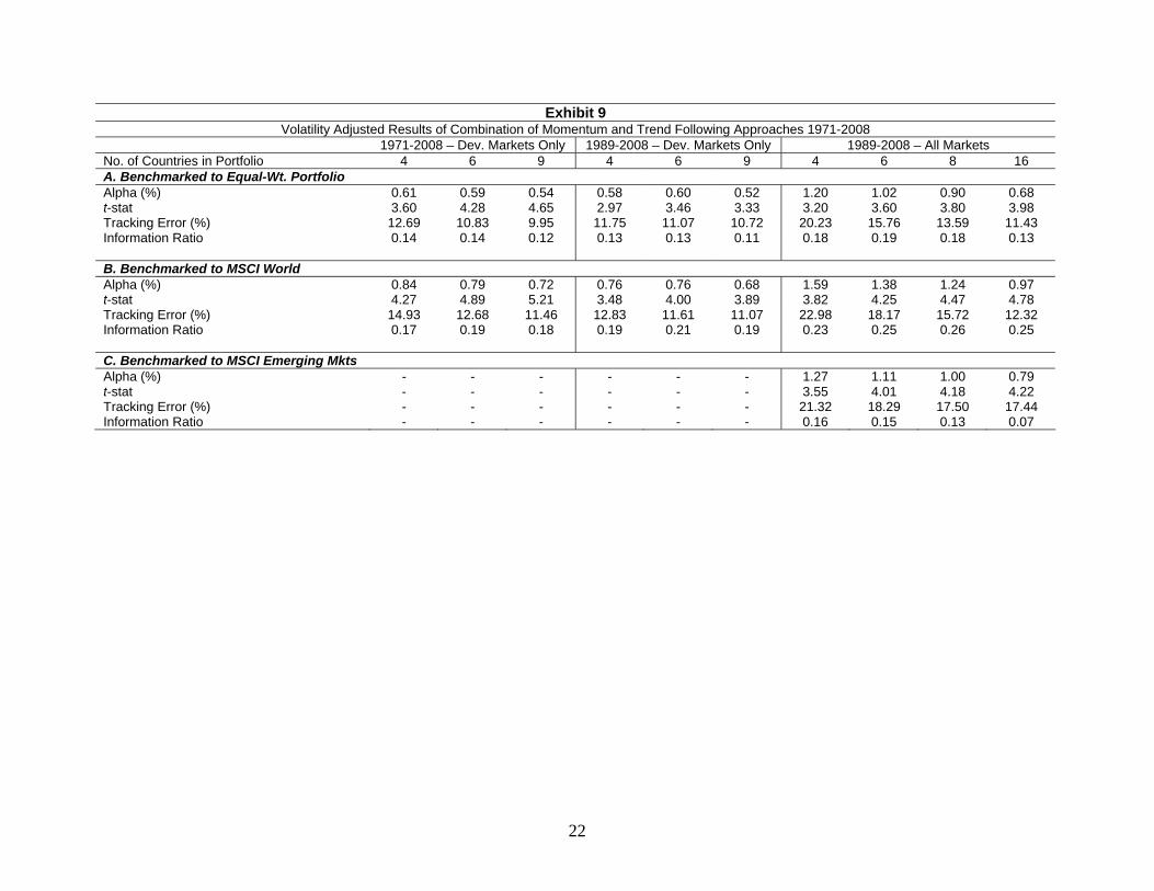
Exhibit 9 Volatility Adjusted Results of Combination of Momentum and Trend Following Approaches 1971-2008

1971-2008 – Dev. Markets Only 1989-2008 – Dev. Markets Only 1989-2008 – All Markets No. of Countries in Portfolio 4 6 9 4 6 9 4 6 8 16 A. Benchmarked to Equal-Wt. Portfolio Alpha (%) 0.61 0.59 0.54 0.58 0.60 0.52 1.20 1.02 0.90 0.68 t-stat 3.60 4.28 4.65 2.97 3.46 3.33 3.20 3.60 3.80 3.98 Tracking Error (%) 12.69 10.83 9.95 11.75 11.07 10.72 20.23 15.76 13.59 11.43 Information Ratio 0.14 0.14 0.12 0.13 0.13 0.11 0.18 0.19 0.18 0.13 B. Benchmarked to MSCI World Alpha (%) 0.84 0.79 0.72 0.76 0.76 0.68 1.59 1.38 1.24 0.97 t-stat 4.27 4.89 5.21 3.48 4.00 3.89 3.82 4.25 4.47 4.78 Tracking Error (%) 14.93 12.68 11.46 12.83 11.61 11.07 22.98 18.17 15.72 12.32 Information Ratio 0.17 0.19 0.18 0.19 0.21 0.19 0.23 0.25 0.26 0.25 C. Benchmarked to MSCI Emerging Mkts Alpha (%) - - - - - - 1.27 1.11 1.00 0.79 t-stat - - - - - - 3.55 4.01 4.18 4.22 Tracking Error (%) - - - - - - 21.32 18.29 17.50 17.44 Information Ratio - - - - - - 0.16 0.15 0.13 0.07

22