EXCUSE ME, DO YOU SPEAK ENGLISH?

AN INTERNATIONAL EVALUATION

Ester Núñez de Miguel

Master Thesis CEMFI No. 1404

December 2014

CEMFI Casado del Alisal 5; 28014 Madrid

Tel. (34) 914 290 551. Fax (34) 914 291 056 Internet: www.cemfi.es

This paper is a revised version of the Master's Thesis presented in partial fulfillment of the 2012-2014 Master in Economics and Finance at the Centro de Estudios Monetarios y Financieros (CEMFI). I am greatly indebted to Samuel Bentolila for his exceptional supervision, guidance and support. I would also like to thank Professors Diego Puga, Pedro Mira, Manuel Arellano, Monica Martinez-Bravo and all participants in the thesis presentations for their helpful and useful comments. Special thanks also to Felipe Carozzi and Jan Bietenbeck for their help and suggestions about how to improve this work, to Ines Berniell for her patience and help with the data, and to Gustavo Fajardo for the long hours of discussion about politics and policy evaluation, providing me great insights. Finally to my classmates, family and friends, who gave me the strength to continue during these two years, especially to my sister Alicia. Special thanks also to INEE for providing me the data. All errors are on my own.

Master Thesis CEMFI No. 1404

December 2014

EXCUSE ME, DO YOU SPEAK ENGLISH? AN INTERNATIONAL EVALUATION

Abstract Globalization and market integration have made languages an essential tool for worldwide communication. Nowadays, English knowledge is spread internationally, its importance is growing, and educational systems introduce students in English learning at an increasingly early age. However, until now, very little was known about which the determinants of English competences are, which differences are linked to country specific factors and which policy educational measures can be taken to improve the English level of students at the end of compulsory education. This paper uses data from the European Survey of Language Competences (ESLC), which allows to make the first study that addresses these queries. By making use of an educational production function, where the `outcome' is the level of English acquired in the evaluated competences, we can infer which the determinants of English performance are at the end of compulsory education. English class size is a particularly important feature of the educational systems because it can be quite easily modified by policy makers. Following Woessmann (EP, 2005) class size European study in sciences cognitive skills, and implementing similar techniques, previously developed by Angrist and Lavy (QJE, 1999), we obtain a statistically significant causal result: bigger English classes perform better on average than smaller ones in Reading and Writing competences. Ester Núñez de Miguel Banco Santander ester.nunez@gruposantander.com

1 Introduction

One of the main interests of economists in educational topics is directly linked

to human capital accumulation, which determines the labor market earnings of

an individual. Human Capital depends on many factors and, globally speaking,

it accumulates first through learning and secondly by practical experience in the

labor market. Therefore, the role of Education as the first source of human capital

accumulation is very relevant from an Economic perspective.

English knowledge covers many different skills, the most widely emphasized

are Listening, Reading, Writing and Speaking. The development of each skill can

be acquired through different teaching techniques and language contact. Lan-

guage contact can also be performed by several activities which can affect some

skills more than others. For example, reading English books can improve Read-

ing and Writing, but not necessarily Speaking or Listening skills. On the other

side, watching not dubbed English movies can improve Listening but not neces-

sarily Reading or Writing skills. Therefore, at the end of compulsory education,

students English level is a multi-skill acquired knowledge, which depends on dif-

ferent learning procedures given to the student by their English teachers, home

and school environment, the implicit ability of the individual in foreign languages

and the contact with the English language that the student could have.

International tests like the Programme for International Student Assessment

(PISA) and Trends in International Mathematics and Science Study (TIMSS) pro-

vide data on common assessment tests carried out all over the World, which allow

us to understand the importance of various factors determining the achievement

and the impact of skills on economic and social outcomes. The European Survey

of Language Competences (ESLC) is the fist survey that provides a common as-

sessment of several English skills in a 13 European educational systems sample.

The ESLC was carried out in 2011 and has the same approach as previous inter-

national tests: it aims at measuring how much English knowledge students have

acquired by the end of compulsory education. It evaluates English proficiency in

Listening, Reading and Writing skills. Speaking was not evaluated and therefore,

it is out of the scope of this study.

I begin my analysis of the determinants of English performance by building an

2

appropriate educational production function. In this function, cognitive skills are

understood as the outcome of a production process, where inputs are the student

characteristics, family background and school and institutional factors, which are

combined to create the output. The educational production function is improved

in order to take into account factors that affect languages specifically, such as

family language controls, which measure the proximity of native European lan-

guages to English. Also, several robustness checks are provided to guarantee that

my estimations are sufficiently accurate in the three evaluated skills.

The second part of my analysis focuses on a very significant determinant that

was found in the educational production function and robustness checks: the

positive and significant effect that English class size has on the three evaluated

English skills. This implies that bigger English classes perform better on average

than smaller ones. This result goes in line with other positive class size effects

found using least squares methods in European data such as Woesmann (2005),

who showed a similar positive effect of class size in science proficiency using TIMSS

data on 12 European school systems.

Least squares coefficients are very likely to be biased due to endogeneity. To

address this important concern, and taking into account that 9 out of 13 countries

in the ESLC sample have maximum class size regulations, I build an instrument

in line with Angrist and Lavy (1999) Maimonides’ rule. What Angrist and Lavy

(1999), Hoxby (2000) or Woessmann (2005) obtained, after using Intrumental

Variables (IV) estimation on the class size effect estimates, was that the class size

coefficients turned negative or no longer statistically significant. Performing IV

estimation on the three ESLC evaluated skills gives us a surprising result: positive

class size effects are obtained in France, Sweden and pooled Countries in Read-

ing and Writing skills. No significant effect for English class size was obtained

in Listening skills. Contrary to what has been believed so far, bigger classes do

not necessarily perform worse in all cognitive skills and, on the contrary, perform

better in Reading and Writing English skills.

To complete this study, I provide the optimal class size in the three skills.

It is obtained by a functional form modification of the English class size in the

estimation of the educational production function. Reading and Writing English

3

skills present an optimal class size of 35 and 33 respectively, which are bigger than

the ones implemented by the maximum class size regulations across Europe. This

study provides causal results which have important Policy implications.

The remainder of the paper is organized as follows. Section 2 describes the

ESLC data, and provides a descriptive analysis of the test results by country.

Section 3 presents the educational production function used to obtain the deter-

minants of English performance, as well as some robustness checks. Section 4

provides a deeper study of English class size by country using OLS and IV es-

timation methods. A detailed description of the instrument and its strenght is

provided. Section 5 gives the optimal class size in each of the three evaluated

skills. Section 6 concludes.

2 The Data

The empirical analysis uses data from the European Survey of Language Com-

petences (ESLC), an European foreign language evaluation test that was carried

out in February 2011. The ESLC was designed to collect information about the

foreign language proficiency of students in the last year of lower secondary ed-

ucation or the second year of upper secondary education, so that student ages

vary from 14 to 16 years old. Fourteen European countries participated in the

survey, and each country was evaluated in two languages, the two most taught

out of the five most widely taught European languages: English, French, German,

Italian and Spanish. The participating countries were Belgium, Bulgaria, Croatia,

Estonia, Greece, France, Malta, Netherlands, Poland, Portugal, Slovenia, Spain,

Sweden and UK-England. Belgium was subdivided into the three educational

systems that it has, and therefore the sample is composed by 14 countries or 16

educational systems. There were two separate samples for the first and second

foreign languages evaluated within each country, so each student was tested in

one language only.

My study uses the first target language sample since 13 educational systems

were evaluated in English as the first target language. This sample has 27,641

observations of which 23,358 correspond to English. I exclude from my study the

educational systems that were not evaluated in English as the first target lan-

guage: UK-England and the Flemish and German regions of Belgium. In what

4

follows, unless I specify the opposite, when I mention Belgium I will be referring

to the French community of Belgium, which is the only region that I include in

my sample.

The ESLC intends to assess students’ ability to use the language purposefully,

in order to understand spoken or written tests, or to express themselves in writ-

ing. The test evaluates three language skills: Listening, Reading and Writing.

Each student was assessed in two out of these three skills and also completed

a contextual questionnaire (SQ). The results of the survey tests are reported in

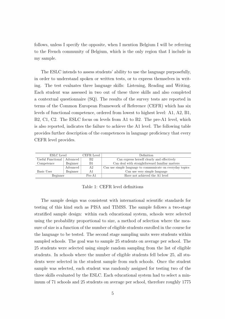
terms of the Common European Framework of Reference (CEFR) which has six

levels of functional competence, ordered from lowest to highest level: A1, A2, B1,

B2, C1, C2. The ESLC focus on levels from A1 to B2. The pre-A1 level, which

is also reported, indicates the failure to achieve the A1 level. The following table

provides further description of the competences in language proficiency that every

CEFR level provides.

ESLC Level CEFR Level DefinitionUseful Functional Advanced B2 Can express herself clearly and effectivelyCompetence Beginner B1 Can deal with straightforward familiar matters

Advanced A2 Can use simple language to communicate on everyday topicsBasic User Beginner A1 Can use very simple language

Beginner Pre-A1 Have not achieved the A1 level

Table 1: CEFR level definitions

The sample design was consistent with international scientific standards for

testing of this kind such as PISA and TIMSS. The sample follows a two-stage

stratified sample design: within each educational system, schools were selected

using the probability proportional to size, a method of selection where the mea-

sure of size is a function of the number of eligible students enrolled in the course for

the language to be tested. The second stage sampling units were students within

sampled schools. The goal was to sample 25 students on average per school. The

25 students were selected using simple random sampling from the list of eligible

students. In schools where the number of eligible students fell below 25, all stu-

dents were selected in the student sample from such schools. Once the student

sample was selected, each student was randomly assigned for testing two of the

three skills evaluated by the ESLC. Each educational system had to select a min-

imum of 71 schools and 25 students on average per school, therefore roughly 1775

5

(71x25) students were sampled. In terms of data quality standards, two minimum

participation rates were determined: for originally sampled schools a minimum

participation of 85% of the schools and a minimum participation of 80% of the

sampled students per school were required. The ESLC Principal Questionnaire

(PQ) and Teacher Questionnaire (TQ) were self selecting: schools principals and

English language teachers of the sampled students of the schools were invited to

fill in the Questionnaires. There was no official participation criterion for the

teachers and principals and the response rate was low.

In order to avoid frustration and boredom and get a higher quality measure of

the student English level per skill, a routine test previous to the skill evaluation

assigned each student to a test level: A1-A2, A2-B1, B1-B2. After the assignment,

each student did 5 tasks per skill, but since each task measures only within a

limited range of level, unless an adjustment is made, task results will not be

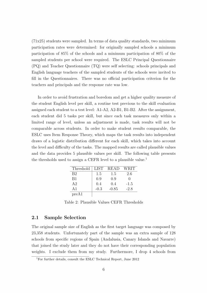
comparable across students. In order to make student results comparable, the

ESLC uses Item Response Theory, which maps the task results into independent

draws of a logistic distribution different for each skill, which takes into account

the level and difficulty of the tasks. The mapped results are called plausible values

and the data provides 5 plausible values per skill. The following table presents

the thresholds used to assign a CEFR level to a plausible value.1

Threshold LIST READ WRITB2 1.5 1.5 2.6B1 0.9 0.9 0A2 0.4 0.4 -1.5A1 -0.3 -0.85 -2.8preA1

Table 2: Plausible Values CEFR Thresholds

2.1 Sample Selection

The original sample size of English as the first target language was composed by

23,358 students. Unfortunately part of the sample was an extra sample of 128

schools from specific regions of Spain (Andalusia, Canary Islands and Navarre)

that joined the study later and they do not have their corresponding population

weights. I exclude them from my study. Furthermore, I drop 4 schools from

1For further details, consult the ESLC Technical Report, June 2012

6

Sweden and Bulgaria where no student completed the Student Questionnaire (SQ)

or only half of the sampled students did complete the Questionnaire. I also drop

174 students who did not complete the SQ but they were evenly distributed across

the schools participating in the survey. Thus, the final sample consists of 20,192

students in 915 schools in 13 educational systems.

2.2 Descriptive Analysis

A descriptive analysis of the results, provided by the mean performance per skill

and country, allows us to rank countries by performance. Countries are ordered

following the position they got in mean Reading which is the same rank as in

mean Writing skills. The following table provides mean plausible values per coun-

try and per skill, its assigned CEFR level and the position they got among the 13

participating countries.

Mean Listening Mean Reading Mean WritingCountry Plaus.Val CEFR Rank Plaus.Val CEFR Rank Plaus.Val CEFR TotalMalta 2.36 B2 1 2.10 B2 1 2.63 B2 1,586Sweden 2.33 B2 2 2.03 B2 2 1.66 B1 1,513Estonia 1.56 B2 4 1.51 B2 3 1.22 B1 1,580Netherlands 1.79 B2 3 1.19 B1 4 0.75 B1 1,760Slovenia 1.45 B1 5 0.90 B1 5 0.31 B1 1,422Greece 0.79 A2 7 0.74 A2 6 0.24 B1 1,177Croatia 1.07 B1 6 0.64 A2 7 -0.10 A2 1,649Belgium fr 0.38 A1 11 0.44 A2 8 -0.95 A2 1,503Bulgaria 0.69 A2 8 0.42 A2 9 -1.17 A2 1,719Spain 0.15 A1 12 0.30 A1 10 -1.51 A2 1,583Poland 0.48 A2 10 0.25 A1 11 -1.60 A1 1,645Portugal 0.61 A2 9 0.24 A1 12 -1.70 A1 1,563France -0.04 A1 13 -0.13 A1 13 -2.42 A1 1,492Total 20,192

Table 3: Mean Test Results by Country

The following graph summarizes the table results. We can see that the Listen-

ing and Reading thresholds are very similar, since the underlying logistic distri-

bution they follow is very similar as well. The mean English results for European

countries are pretty low except for Malta, Sweden, Estonia and the Netherlands.

After an average of 9 years of compulsory education, which includes in most of

the countries the same number of years of English compulsory learning, half of

the countries are unable to reach mean results above B1, which determines the

lowest level for a useful functional competence.

7

However there is a significant variability of the results across countries. At a

glance we can see that the top ranking countries are small countries, with a native

language that is only spoken within those countries. At the botton of the rank,

big countries are located, which also have native languages spoken widely across

the World, like Spain and France.

Figure 1: Mean Test Results by Country

Due to this significant variability of the results across countries, I’d like to

study what factors are behind, exploring what are the main determinants of En-

glish proficiency at the end of compulsory secondary education. To do it, I am

going to use the contextual information provided by the Student Questionnaire

and national information, in order to infer which factors are relevant, which fac-

tors’ effects differ from previous research of other skills previously evaluated in

other international tests such as PISA, TIMSS and PIRLS, and try to do a policy

evaluation that allows us to improve the English results in future.

In the rest of my analysis I will use the plausible value results, since they

measure the level of performance in the evaluated English skills, knowing that

they have a CEFR level associated.

8

3 The Education Production Function

One of the main interests of economists in Educational topics is directly linked

to Human Capital accumulation, which determines the labor market earnings of

an individual. There are several factors which determine the human capital of

an individual: the education acquired, the personal and labor market experience,

the family background and the intrinsic ability of the individual, which is also a

determinant of the other Human Capital input factors. Globally speaking, human

capital accumulates first through learning and second by practical experience in

the labor market. Therefore the role of Education as the first source of human

capital accumulation is very relevant from an Economic perspective.

Nowadays English knowledge has become a very valuable skill and a prerequi-

site for success in the labor market. Apart from work purposes, research, global

media and tourist information are most of the times carried out or given in English,

and therefore, its knowledge has become relevant also for educational purposes and

leisure time.

During the past decade, the economic literature has made use of international

tests of educational achievement to analyze the determinants and impacts of cog-

nitive skills. International tests assess what students know, cognitive skills, as

opposed to how long they have been in school or what is the value added of an

extra year of a professor. This testing approach intends to measure the knowledge

of the students for practical purposes, and the ESLC has the same approach: it in-

tends to assess students’ English ability to use language purposefully. It measures

how much English knowledge students have acquired by the end of lower sec-

ondary education, or equivalently, by the end of compulsory education. It does so

by measuring the global proficiency in English after an average of 9 years of study.

The ESLC was carried out in 11 of the sampled countries in the last year

of lower secondary education, and in Bulgaria and Belgium at the second year

of upper secondary education. The sample criteria intended to avoid significant

differences in the study level of the sampled students, and only very few excep-

tions were allowed. The Bulgarian educational system presents the characteristic

that the primary education only lasts 4 years, while in the rest of the sampled

countries the general pattern is 6 years of primary education, and since the lower

9

secondary education lasts 4 years, Bulgarian kids at the end of second year of

upper secondary education have the same age as the Spanish kids who, at the

end of lower secondary education, have completed 6 of primary and 4 of lower

secondary years of education. In the Belgian case, the primary education lasts 6

years, but the lower secondary only 2 and the English onset is done at the end of

primary education. Therefore, for the explained reasons, an exception was made

in both cases.2

Generally speaking, homogeneity across educational systems in Europe is not

present. There are substantial differences in the age at the beginning of compul-

sory primary education, in the existence or not of pre-primary education, in the

duration of primary and lower secondary education and on the English age onset

at school.

3.1 The model

The model underlying the literature of the determinants of international educa-

tional achievement resembles the following educational production function:

Sisc = β0 + β1Fi + β2Ris + β3Ic + β4Ai + εisc

where Sisc are the test scores in the Listening, Reading and Writing skills

evaluated, Fi captures student and family background characteristics, Ris is a

measure of school resources, Ic captures institutional features, Ai is the individual

ability of the student and εisc is a logistically distributed error, since the outcome

variable follows a logistic distribution.

There are several ways to exploit the cross country variation. The first one con-

sists of the estimation of similar education production functions within different

countries, which exploits country level observations, as performed by Hanushek

and Kimko (2000).

The second possibility is to exploit the broad array of institutional differences

that exists across countries to estimate a pooled multivariate cross-country educa-

tion production function in the same way that Woessmann, Luedemann, Schuetz

and West (2009) did using PISA 2003 data. This second approach is the one that

2For more details, consult the Final Report European Survey of Language Competences.

10

I will follow. It combines micro data on student achievement and institutional

information to obtain the effect of the determinants of English skill performance

at an European level.

This cross-country comparative approach provides advantages. First, it ex-

ploits institutional variation that does not exist within countries, by pooling ob-

servations that belong to different institutional systems these institutional differ-

ences can be estimated, which is impossible in within country estimation. Second,

it reveals whether any result is country specific or more general. Third, since inter-

national European data presents much wider variation than any sample belonging

to a specific country, this international variation implies more statistical power to

detect the impact of specific factors on student outcomes. Therefore, it allows for

the determination of specific factors that affects students outcomes internationally.

The cross-sectional nature of this estimation allows only for a descriptive inter-

pretation of which are the determinants of English performance, since the implicit

individual ability can only be controlled partially by the student and family back-

ground characteristics.

3.2 Specification

The following section provides a general specification of the variables included

in the model in each of the factors which determine the educational production

function.

The student and family background characteristics include: on one hand, stu-

dent characteristics such as exact age at the beginning of February, gender, Im-

migrant status, which takes the value 1 if the student reports to have been born

in another country, and Repetition, which is an indicator variable that takes the

value 1 if the student has repeated at least one grade; on the other hand, fam-

ily background characteristics such as: if the student’s parents hold a university

degree, if they are white, blue or pink collar workers, their parent’s knowledge

of English, the number of books the student has at home, if the student uses

English at home and if the student has English as one of his/her mother tongues

(learnt before being 5 years old). Apart from the White Collar indicators for both

parents, a Blue Collar Father indicator and a Pink Collar Mother indicator are

11

included. Pink collar are occupations related to services, which have traditionally

been done by women such as secretaries, hairdressers, nurses, etc. The reason

why I include Pink Collar mother rather than Blue Collar mother, that has been

traditionally the included sector in international studies, is as follows. The service

sector weight has grown in the last few decades in developed economies. Since

this new source of employment and growth is mainly related with services, women

have a competitive advantage with respect to men in this sector and it could be

a reason for the increasing female participation in the labor force during the last

decades. Therefore, it seems natural to include a group of occupation that takes

into account this fact and has, until now, not been used in previous international

studies. The Economic, Social and Cultural Status (ESCS) index is comprised

of three components: home possessions (such as number of bathrooms and TVs,

among others items, that are an approximate measure of the household wealth),

parental occupation and parental education expressed in years of schooling. This

compound index is provided by the ESLC as it is always the case in other inter-

national tests.

The school resources are all variables related to the school, but reported by the

student. It includes: the number of years of English study at school since the be-

ginning of primary education, early onset at school (indicator variable that takes

the value 1 if the student studied English at school in pre-primary education),

English lesson time per week, English class size, ancient languages (indicator vari-

able that takes the value 1 if the student has studied ancient languages) and the

number of foreign languages studied at school reported by the student. In my

specification I include the English class size in logarithms because it is the func-

tional form that better captures the fact that an extra student has proportionally

higher impact on smaller classes.

The institutional variables include information such as the GDP per capita in

purchasing power parity of 2010 in prices of 2005, Educational Expenditure on

secondary education per student in 20103, the country population at the begin-

ning of 2011, an indicator variable if the TV in English is not dubbed, External

Exit Exams (if the students have to perform an external exit exam to get their

lower secondary education degree), which according to Eurydice4 it is the case

3GDP per capita and Educational Expenditure are given in 2005 prices.4Network that provides information and analyses of European education systems and policies.

12

for Malta, France, Portugal, Netherlands, Poland and Estonia; and Multilingual

region, that is an indicator variable that takes the value one if the school was

located in one of the five multilingual regions sampled: four in Spain and one in

Estonia. This last variable is a regional one.

Finally, I include a set of family language controls. Most languages in Europe

can be grouped by family language, which gathers languages by their proximity.

In my sample, except of Estonian and Greek which do not belong to any of

the main European family languages, the rest of the languages can be grouped

by families: Germanic, which English belongs to and also includes Dutch and

Swedish, Romance, which groups all the Latin origin languages: French, Maltese,

Portugese and Spanish; and Slavic which includes Bulgarian, Croatian, Polish

and Slovenian.5

3.3 Empirical results

The data provides 5 plausible values per evaluated skill, which are independent

draws of a logistic distribution that takes into account the difficulty and level of

the performed tasks. Due to this independence across plausible values, the mean

of the 5 plausible values is a good estimator of the overall skill performance of

the student. Therefore, the plausible values are transformed into student means

per skill. Table 4 provides some descriptive statistics, weighted by the student’s

sampling probability, of the outcome variables that are going to be used in the

following estimation.

From the original initial sample of 20,192 observations, 5,228 observations are

lost due to missing values in the Student Questionnaire. Since these observa-

tions with missing values are removed from my estimation, the following weighted

statistics outcomes variables exclude those observations. This table provides the

mean, standard deviation and minimum and maximum values of the outcome

variables that are going to be used in the weighted least-squares estimation. As

we can see, Mean Listening and Mean Reading skills have a very similar distri-

bution, while Mean Writing presents a much more dispersed one. This has to be

taken into account when evaluating the impact of the skill determinants of English

performance.

5The Appendix provides a descriptive summary of all the variables used in the Baseline.

13

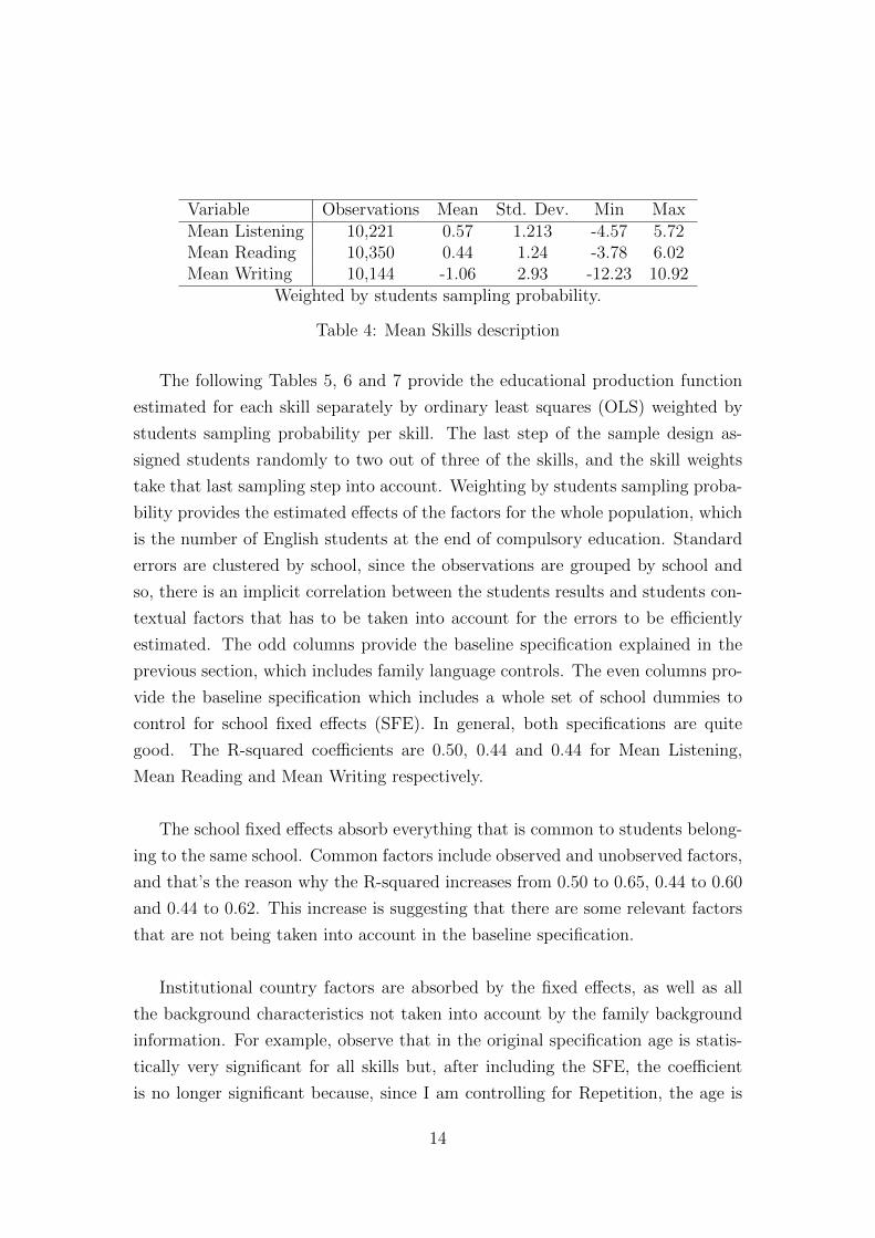
Variable Observations Mean Std. Dev. Min MaxMean Listening 10,221 0.57 1.213 -4.57 5.72Mean Reading 10,350 0.44 1.24 -3.78 6.02Mean Writing 10,144 -1.06 2.93 -12.23 10.92

Weighted by students sampling probability.

Table 4: Mean Skills description

The following Tables 5, 6 and 7 provide the educational production function

estimated for each skill separately by ordinary least squares (OLS) weighted by

students sampling probability per skill. The last step of the sample design as-

signed students randomly to two out of three of the skills, and the skill weights

take that last sampling step into account. Weighting by students sampling proba-

bility provides the estimated effects of the factors for the whole population, which

is the number of English students at the end of compulsory education. Standard

errors are clustered by school, since the observations are grouped by school and

so, there is an implicit correlation between the students results and students con-

textual factors that has to be taken into account for the errors to be efficiently

estimated. The odd columns provide the baseline specification explained in the

previous section, which includes family language controls. The even columns pro-

vide the baseline specification which includes a whole set of school dummies to

control for school fixed effects (SFE). In general, both specifications are quite

good. The R-squared coefficients are 0.50, 0.44 and 0.44 for Mean Listening,

Mean Reading and Mean Writing respectively.

The school fixed effects absorb everything that is common to students belong-

ing to the same school. Common factors include observed and unobserved factors,

and that’s the reason why the R-squared increases from 0.50 to 0.65, 0.44 to 0.60

and 0.44 to 0.62. This increase is suggesting that there are some relevant factors

that are not being taken into account in the baseline specification.

Institutional country factors are absorbed by the fixed effects, as well as all

the background characteristics not taken into account by the family background

information. For example, observe that in the original specification age is statis-

tically very significant for all skills but, after including the SFE, the coefficient

is no longer significant because, since I am controlling for Repetition, the age is

14

virtually the same across students in the same grade and school, and therefore the

SFE absorb the age school characteristic. However, for some other variables the

relative change in the significance of some coefficients is not so obvious and could

point towards between school sorting bias. For example, the Father University

coefficient is very significant in the baseline, but not significant in the SFE specifi-

cation. In this case, the significant change in the estimates suggests that the OLS

estimation suffers from between-school sorting bias. In other words, parents who

have a higher level of education may decide to put their kids in specific schools

which are private or tougher, and parents with lower level of education may not

know about the local schools quality and send their kids to the closest local one.

Therefore, due to this sorting between schools, the educational level of the father

is common across the students, so it is absorbed by the SFE. The same pattern

is observed with Pink Collar mother in Reading or Mother University in Listening.

Globally speaking, coefficients are in general statistically significant. However,

in terms of standard deviations, its effects are very small since only very few have

an equivalent impact to more than a half standard deviation in terms of mean

test scores. For example grade Repetition, that is significant at 1% level, creates a

negative effect that is only equivalent to 0.25 standard deviations lower in Listen-

ing, 0.3 standard deviations lower in Reading and 0.42 standard deviations lower

in Writing scores.

In line with PIRLS studies, girls perform better in Writing skills relative to

boys, although it only provides an advantage equivalent to 0.16 standard devi-

ation higher scores. Immigrant status, which in other international studies has

been always a negative determinant in math and reading skills, is a positive and

significant determinant of Listening skills, equivalent to 0.2 standard deviations

higher scores.

Books at home and ESCS index are, as the literature has shown, a positive and

significant predictor of student performance. Books reference is the lower rank

of books at home, from 11 to 25. We can observe that the higher the number of

books at home, the bigger its effect become, going from an equivalent of 0.13 to

0.25 standard deviations higher in all skills. The ESCS index effect is significant

but its effects is only about 0.1 standard deviations higher scores in all skills.

15

Mean Listening Mean Reading Mean Writing(1) (2) (3) (4) (5) (6)

STUDENTCHARACTERISTICSAge -0.14*** -0.02 -0.09*** -0.02 -0.18** 0.02

(0.028) (0.033) (0.03) (0.029) (0.085) (0.09)Female 0.02 -0.01 0.01 0.004 0.48*** 0.42***

(0.03) (0.03) (0.03) (0.03) (0.08) (0.07)Repetition -0.18*** -0.25*** -0.35*** -0.33*** -1.26*** -1.38***

(0.058) (0.058) (0.056) (0.054) (0.13) (0.16)Immigrant 0.23*** 0.196** 0.10 0.07 0.27 0.073

(0.08) (0.087) (0.08) (0.08) (0.21) (0.22)FAMILYBACKGROUNDBooks 26-100 0.02 0.02 0.08** 0.04 0.39*** 0.32**

(0.045) (0.045) (0.04) (0.04) (0.13) (0.13)Books 101-200 0.16*** 0.13*** 0.25*** 0.18*** 0.66*** 0.5***

(0.0423) (0.04) (0.04) (0.04) (0.12) (0.11)Books>200 0.19*** 0.19*** 0.33*** 0.25*** 0.73*** 0.6***

(0.05) (0.047) (0.05) (0.047) (0.14) (0.13)ESCS index 0.13*** 0.06*** 0.15*** 0.08*** 0.26*** 0.11

(0.03) (0.02) (0.03) (0.027) (0.10) (0.08)Father University 0.085** 0.03 0.09* 0.05 0.28** 0.28**

(0.04) (0.04) (0.047) (0.05) (0.121) (0.112)Mother University 0.113*** 0.049 0.11** 0.08* 0.35*** 0.14

(0.043) (0.04) (0.05) (0.046) (0.106) (0.106)White Collar Father 0.02 0.03 0.04 0.03 -0.12 -0.09

(0.039) (0.039) (0.047) (0.045) (0.117) (0.103)White Collar Mother 0.18*** 0.15*** 0.21*** 0.15*** 0.57*** 0.45***

(0.049) (0.043) (0.049) (0.05) (0.14) (0.4)Blue Collar Father -0.09** -0.07* -0.12*** -0.13*** -0.42*** -0.31**

(0.039) (0.037) (0.04) (0.04) (0.13) (0.12)Pink Collar Mother 0.10*** 0.07** 0.08* 0.03 0.48*** 0.34***

(0.036) (0.034) (0.046) (0.035) (0.129) (0.112)Father English Well 0.16*** 0.12*** 0.15*** 0.10*** 0.48*** 0.31***

(0.035) (0.034) (0.035) (0.035) (0.098) (0.102)Mother English Well 0.04 0.02 0.05 0.05 0.13 0.1

(0.032) (0.032) (0.04) (0.04) (0.099) (0.098)English use at home 0.41*** 0.38*** 0.35*** 0.4*** 0.98*** 1.01***

(0.04) (0.05) (0.05) (0.05) (0.13) (0.12)Early Onset at home 0.23*** 0.16** 0.23*** 0.09 0.41** 0.34**

(0.074) (0.081) (0.08) (0.081) (0.18) (0.17)

Fam.Language Controls yes no yes no yes noSchool Controls no yes no yes no yesObservations 10,221 10,221 10,350 10,350 10,144 10,144R-squared 0.502 0.647 0.443 0.599 0.440 0.623

Clustered robust standard errors by school in parentheses, *** p<0.01, ** p<0.05, * p<0.1Weighted by students sampling probability

Table 5: Student and Family Background

16

Mother and Father University have both a positive and significant impact,

equivalent to 0.1 standard deviations higher scores in all skills. White Collar

Mother has a positive effect in all the skills, varying its effects from 0.15 to 0.2

standard deviations. The fact that only one of the parents affects the kid could

be driven by relative impact or by collinearity due to assortative mating. In fact,

the correlation of parents education expressed in years in the sample is around

0.62 and the parents white collar occupation correlation is around 0.45, which

suggests that assortative mating could be the reason behind this fact. Blue Col-

lar Father presents a negative and significant effect in all English skills, although

its effect is small. Pink Collar Mother is a positive and significant determinant,

whose effect represents 0.1 standard deviation higher scores in all skills. In the

occupational variables I use as a reference of White Collar Father and Blue Collar

Father, unemployed, retired and Pink Collar Father. In the case of the White

Collar Mother and Pink Collar Mother the reference is unemployed, retired and

Blue Collar mother. In each case, I decided to put as a reference the categories

which have fewer number of observations. Parents occupation variables White

Collar and Blue Collar father behave as previously in other international studies:

White Collar parents have a positive and significant effect on student’s scores, and

Blue Collar has a significant negative effect. The Pink Collar mother significant

positive effect is a novel finding.

Estimations in the lower part of Table 5 present variable effects that are specif-

ically related to English, and that have not been used before in previous research

on maths and literature skills. The same pattern observed in White Collar parents

happens with Parents English knowledge, where only the Father knowledge has

a statistically significant positive effect in all skills, which represents scores 0.15

standard deviations higher. Again, these two variables present a correlation of

0.43. English use at home is a positive and significant coefficient which represents

0.33 standard deviation higher scores across all skills evaluated. Early onset at

home, which indicates whether one of the kid’s mother tongues is English, has also

a significant effect in all skills, between 0.15 and 0.2 standard deviations higher.

Not surprisingly, its effect seems to be higher for Listening skills. The interaction

between books and Parents English knowledge, which could capture the fact that

if parents have a high English level, some of the books at the student home could

be in English, did not have any effect, and therefore I excluded it.

17

Table 6 provides estimates of School Information given by the student. As can

be seen, variables are statistically very significant although their effects are all

between 0.05-0.1 standard deviations higher. Particularly remarkable is the fact

that the Ancient Languages indicator provides a 0.16 standard deviations higher

Writing scores.

Mean Listening Mean Reading Mean Writing(1) (2) (3) (4) (5) (6)

SCHOOL INFORMATIONEnglish Hours per Week 0.08*** 0.06** 0.1*** 0.09*** 0.27*** 0.24***

(0.026) (0.029) (0.031) (0.034) (0.067) (0.09)Years English School >5 years 0.03*** 0.03*** 0.05*** 0.05*** 0.08*** 0.07***

(0.006) (0.007) (0.006) (0.006) (0.02) (0.02)Early Onset at School <5 years 0.17*** 0.09* 0.17*** 0.08 0.51*** 0.23*

(0.06) (0.05) (0.06) (0.05) (0.13) (0.12)Number of Foreign Languages 0.11*** 0.10*** 0.11*** 0.10*** 0.21*** 0.09

(0.024) (0.023) (0.026) (0.025) (0.06) (0.07)Ancient Languages 0.07 0.11** 0.13** 0.15** 0.39*** 0.5***

(0.054) (0.046) (0.058) (0.061) (0.14) (0.14)English Class Size logarithms 0.16*** 0.27*** 0.19*** 0.31*** 0.75*** 0.79***

(0.05) (0.056) (0.057) (0.067) (0.17) (0.12)INSTITUTIONALINFORMATIONGDP ppa 2010 per capita -0.07*** -0.06*** -0.18***

(0.02) (0.02) (0.05)Educational Expenditure 2010 0.16*** 0.15** 0.62***

(0.06) (0.06) (0.14)TV English not dubbed 0.16 0.20* 0.47*

(0.10) (0.12) (0.27)Population 2011 -0.11*** -0.06*** -0.20***

(0.02) (0.017) (0.04)Multilingual Region 0.28** 0.08 0.65

(0.13) (0.16) (0.42)External Exit Exams -0.11 -0.35*** -0.67***

(0.078) (0.086) (0.2)Fam.Language Controls yes no yes no yes noSchool Controls no yes no yes no yesObservations 10,221 10,221 10,350 10,350 10,144 10,144R-squared 0.502 0.647 0.443 0.599 0.440 0.623

Clustered robust standard errors by school in parentheses, *** p<0.01, ** p<0.05, * p<0.1Weighted by students sampling probability

Table 6: School and Institutional Information

English class size is expressed in logarithms to account for the fact that an

extra student has higher impact in smaller classes rather than in bigger ones. Its

effect is positive and significant, equivalent to a quarter of a standard deviation

higher in all skills. This implies that bigger classes perform a quarter of a standard

deviation better in all English skills. This surprising result motivates the second

part of my study.

18

Additionally, Table 6 provides the effect of institutional factors on each skill.

The GDP per capita 2010 effect is negative and significant. This is highly re-

markable since the countries which have higher GDP per capita are Sweden and

Netherlands, which have also a higher level of English as shown in Figure 1. Al-

though in any case its effect is very small. Educational Expenditure in 2010 at

secondary is positive and significant, representing between 0.10 to 0.15 higher

standard deviations. TV English not dubbed is positive and significant although

its effect is not significant precisely for the Listening skill, that is the skill that

could benefit more from listening TV in English. The Population coefficient of

2011 expressed in tens of million, goes in the expected direction: bigger countries

have worst results in English skills. In the case of Belgium I have use the popu-

lation of Belgium Wallonia.

Multilingual regions perform positively and significantly better in Listening,

equivalent to 0.25 standard deviations higher scores. Surprisingly External Exit

Exams is negative and significant, this could point to a teaching-to-the-test neg-

ative effect. The fact that the country makes the students do an external exit

exam precisely at the end of that academic year could make students to pay more

attention to the courses that are evaluated by the test. On the other hand, due to

External Exit Exams, English teachers could pay more attention to activities and

English knowledge that are not evaluated by the ESLC which makes a purposeful

use of English evaluation, like vocabulary or grammar. Several interactions have

been tried between country variables such as GDP and its Population and GDP

and TV in English not dubbed at that country, but none of them provided a

statistically significantly effect, and therefore, I removed those interactions from

the especification.

Table 7 provides the Family Language control coefficient estimates used in the

baseline specification of Listening, Reading and Writing from the odd columns pre-

viously commented. The Family Language Germanic control estimate, to which

English belongs and also groups Dutch and Swedish, is positive and highly sig-

nificant across all skills. It is the equivalent to a complete standard deviation

higher scores in Listening, 0.75 standard deviations in Reading and 0.2 standard

deviations in Writing. Romance family language is negative and significant, and

it is equivalent to 0.2 to 0.5 standard deviation less in scores across all skills.

19

Slavic languages also perform the equivalent to 0.2 and 0.3 standard deviation

less in Reading and Writing skills. This results clearly quantify the proximity of

languages with respect to English and illustrate the comparative advantage that

Dutch and Swedish kids have with respect to other family languages.

Mean Listening Mean Reading Mean WritingFamily Language Controls (1) (3) (5)

Germanic 1.25*** 0.92*** 0.65**(0.121) (0.125) (0.289)

Romance -0.29*** -0.28*** -1.57***(0.103) (0.109) (0.247)

Slavic -0.07 -0.32*** -0.83***(0.0835) (0.0944) (0.209)

Observations 10,221 10,350 10,144R-squared 0.502 0.442 0.440Clustered robust standard errors by school, *** p<0.01, ** p<0.05, * p<0.1

Weighted by students sampling probability

Table 7: Family Language Controls

3.4 Robustness Check 1: Country Controls

Table 11 provides again the least squares weighted specification. The odd columns

provide the baseline specification that was in the odd columns in the previous sec-

tion, with family language controls, and the even columns provide the baseline

specification which includes a whole set of country dummies to control for country

fixed effects (CFE). As before, the fixed effects absorb everything that is common

to students belonging to the same country. Common factors include observed and

unobserved factors, but this time, contrary to the section where we used the SFE,

the R-squared improvement is tiny: from 0.502 to 0.508, 0.442 to 0.448 and 0.44

to 0.441. This little increase suggests that the country effects affecting English

skill performance are mostly taken into account by the baseline specification: the

observed factors can almost totally explain the country factors that are affecting

the results.

Notice that the results with CFE, contrary to the SFE specification, do not

lose significance in any variable and coefficients do not change much with respect

20

to the baseline model with family language controls. Therefore, they confirm that

the results from the original specification have only little country bias, and are

robust enough to explain the determinants of English performance.

3.5 Robustness Check 2: Same Student Regressions

In previous regressions, I was only taken into account students that had been

evaluated in the skill we wanted to study. Since students were randomly allocated

to two out of three evaluated skills, the determinant expressed the average effect

of the factors on English skills, knowing that the students are not the same in

all specifications. Therefore, it will be interesting to check if there are signifi-

cant changes between determinants when we take into account the same student

performing different skills. In other words, I will group students by types, each

type corresponding to every possible combination of the two out of three evalu-

ated skills: Type 1 if the student was evaluated in Listening and Reading, Type

2 if the student was evaluated in Listening and Writing and Type 3 if the stu-

dent was evaluated in Reading and Writing. The drawback of this estimation is

that this focus on smaller groups reduces the sample size in each of the regressions.

From the original sample there were 493 students that were only evaluated

in one skill, therefore, they are excluded from the specifications of this section.

Table 12 and 13 show the observations used to perform the estimates since obser-

vations that have at least one missing value on the variables used for estimation

are removed. Table 12 divides the sample by country, and each country by types.

Table 13 provides a descriptive summary of the outcomes performed by each of

the student types. We can see that the descriptive statistics of the outcomes do

not change significantly from the original total mean skill descriptive statistics

reported in Table 4, which is a good signal, since the allocation of kids to different

skills seems to be purely random.

Table 14 reports the results of these regressions. As it can be seen, these

estimates are very similar to the ones obtained previously: determinants in general

are very significantly different from 0, but they represent little individual impact

in terms of standard deviations in scores. For the sake of brevity, I will only

comment results that differ from previous ones.

21

Repetition, that was previously significant, negative and equivalent to a quar-

ter of a standard deviation in terms of scores is now insignificant in the Listening

skill of the first type. It represents a half of a standard deviation less in writing

of Type 2 and represents a significant quarter standard deviation less in terms of

scores in Reading and Writing of Type 3. Immigrant status is no longer significant

in Listening for the Second Type. Surprisingly, Father and Mother university as

well as Pink Collar Mother are not significant for the Type 1 student. The rest of

family background behave as before in terms of impact and significance. School

information behaves also as before in terms of impact and significance. In the

institutional information the Multilingual region indicator, that previously gives

only a positive advantage equivalent to a quarter of a standard deviation extra

scores in Listening, are present now also as well in Writing for Type 3 students.

Therefore, globally speaking, results do not change much from the initial spec-

ification. So, we can conclude that the original specification results are robust to

CFE and to sample reductions. The specified multivariate education production

function has enough statistical power to perform an accurate descriptive analyses

of which are the determinants of English skills.

22

4 English Class Size

Previous sections have shown, under many different specifications, that English

Class size in logarithms reported by students, is a positive and very significant

determinant of English performance for all English skills evaluated. The effect of

a bigger class gives students around a quarter of a standard deviation of extra

score in all evaluated skills. This means that bigger classes perform better on

average than smaller ones. I used the natural logarithms specification because a

change in class size by one student is proportionately larger for smaller classes,

as was already noticed by Hoxby (2000). Hoxby (2000) shows that simple least-

squares estimates are biased towards showing positive effects of smaller classes

in the US state of Connecticut. While her estimated least-squares coefficients

are negative and statistically highly significant, her identification strategy using

exogenous class-size variations to estimate causal effects yield ”rather precisely

estimated zeros”.

However, results are very different in most European countries. As Woesmann

(2005) showed using TIMSS data, in 12 European school systems, class size is sta-

tistically significant positively related to maths performance using least-squares

estimation in all countries. The positive and significant coefficients of class size

obtained in this study, corroborate what previous studies have found related to

the positive effect of class size on scores of the European countries.

The problem with least squares conventional estimates is that school resources

in general, and class sizes in particular, are not only a cause but also a conse-

quence of student achievement or of the unobserved factors related to student

achievement. Class sizes depend on choices by politicians, administrators and

parents, which may be related to the level of performance achieved. Therefore,

the least squares coefficients are very likely to be biased, the direction of which

is ambiguous a priori. However, it is highly remarkable that the bias seems to go

in the opposite direction from the bias found using US data. While in the United

States, the resource allocation of schools, measured by class size, is strongly re-

lated to family background in a regressive way, due to the unique US features of

decentralized education finance and considerable residential mobility, many other

forces seem to be at play in Europe that give rise to a compensatory resource

allocation, as observed by West and Woessmann (2003).

23

4.1 Instrumenting English Class Size

The ideal way to overcome endogeneity problems is to perform explicit experi-

ments, which generates exogenous variation in class size by randomly assigning

students to different sized classes. To my knowledge, no experiment of this kind

has been carried out in Europe yet. The second possibility to identify causal

class-size effect is to use quasi-experimental strategies. The best known example

of it was introduced by Angrist and Lavy (1999). Angrist and Lavy used a max-

imum class size rule in Israel, which is popularly known as Maimonides’ rule, to

generate an exogenous predictor of the class size, which is used as an instrument

for the actual class size. Maximum class size rules induce a nonlinear and non

monotonic relationship between grade enrollment and class size, which generates

rule-induced discontinuities that creates the exogenous variation that can be ex-

ploited to obtain the causal effect of class size on test scores.

For the sake of simplicity, I will explain what the class size regulation induces

in schools with an example. Imagine we have a school in a country which has

a maximum class size regulation of 25 students. At the beginning of the school

year, that school has a cohort size of 25 students which are allocated to the unique

class that the school has, since the number of students does not force the school

to open two classes. However, the number of students that the school has by

cohort is a combination of multiple choice decisions taken first, by the parents

of the students, who decided to move to that neigbourhood and to matriculate

their kids in that school; second, by the kids effort, which have made possible

for them to pass all the previous courses and third, by the administrations, who

have chosen the materials and level required for students to pass previous courses.

Due to such combination of endogenous choices, those 25 students are together

in the unique class offered by the school. Now imagine that instead of 25, the

school has 26 students at the beginning of the year, and therefore, the school is

forced to open two classes of size 13. We can see that the only difference between

being in a class of 25 or 13 is just that a last additional kid appeared randomly in

the second scenario. The difference between scenarios is just due to the maximun

class size regulation, which induces a non linear and non monotonic difference

between cohorts. Since such large drops in class size come about solely due to

regulation, it can be argued that they are exogenous to students performance and

purely random. If so, we can use the exogenous variation created by the rule

24

induced discontinuities to build the Predicted Class Size function and use it as an

instrument of the actual class size in IV estimation. If students’ test results are

different in classes that only differ in terms of this maximum class size rule, this

can be attributed to a causal effect of class size.

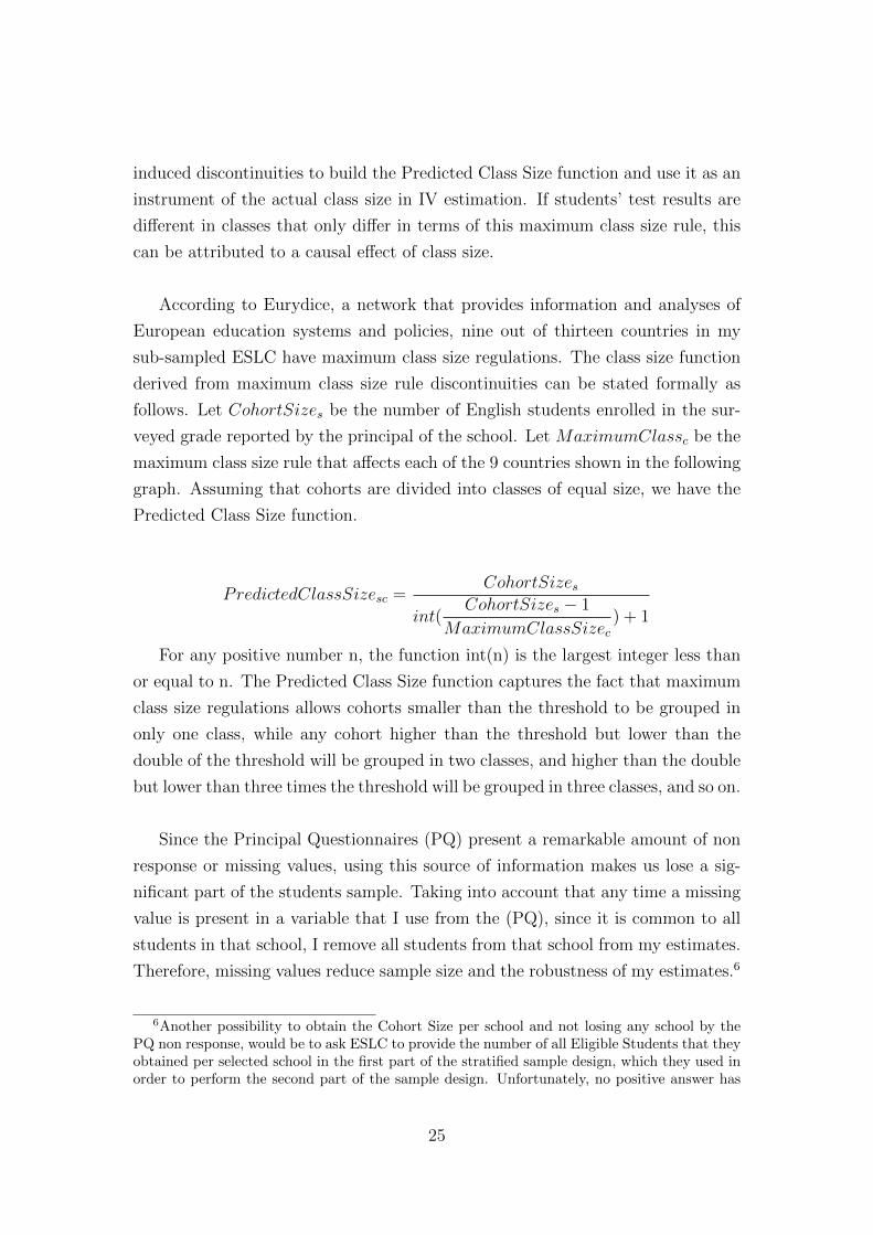
According to Eurydice, a network that provides information and analyses of

European education systems and policies, nine out of thirteen countries in my

sub-sampled ESLC have maximum class size regulations. The class size function

derived from maximum class size rule discontinuities can be stated formally as

follows. Let CohortSizes be the number of English students enrolled in the sur-

veyed grade reported by the principal of the school. Let MaximumClassc be the

maximum class size rule that affects each of the 9 countries shown in the following

graph. Assuming that cohorts are divided into classes of equal size, we have the

Predicted Class Size function.

PredictedClassSizesc =CohortSizes

int(CohortSizes − 1

MaximumClassSizec) + 1

For any positive number n, the function int(n) is the largest integer less than

or equal to n. The Predicted Class Size function captures the fact that maximum

class size regulations allows cohorts smaller than the threshold to be grouped in

only one class, while any cohort higher than the threshold but lower than the

double of the threshold will be grouped in two classes, and higher than the double

but lower than three times the threshold will be grouped in three classes, and so on.

Since the Principal Questionnaires (PQ) present a remarkable amount of non

response or missing values, using this source of information makes us lose a sig-

nificant part of the students sample. Taking into account that any time a missing

value is present in a variable that I use from the (PQ), since it is common to all

students in that school, I remove all students from that school from my estimates.

Therefore, missing values reduce sample size and the robustness of my estimates.6

6Another possibility to obtain the Cohort Size per school and not losing any school by thePQ non response, would be to ask ESLC to provide the number of all Eligible Students that theyobtained per selected school in the first part of the stratified sample design, which they used inorder to perform the second part of the sample design. Unfortunately, no positive answer has

25

Table 15 illustrates how many observations remain available after removing

missing values of the Cohort Size and after also removing the missing values that

come from the SQ information. The last column shows the number of available

observations to perform the second part of my study.

Figure 2 depicts countries affected by maximum class size regulations. Num-

bers in brackets denote the maximum class size per country. The graph plots the

average class size in a grade against the number of English students that are in

that grade, i. e. cohort size, reported by the principal of the school. The red

straight lines depict the average class size that would be predicted by an strict

implementation of the maximum class-size rule.

Figure 2: Predicted and actual average class size by grade enrolment

Figure 3 depicts an amplified graph of Portugal from Figure 2. The continu-

ous blue line shows the relation between the mean of the actual English class size

reported by students and the English cohort size of the grade that students belong

been given yet to me to this petition, and I have to work using the PQ available information.

26

Figure 3: Predicted and actual average class size by Cohort size in Portugal

to, reported by the principal. The dashed red line plots the Predicted Class size

function taking into account the Cohort Size reported by the principal. The blue

horizontal dashed lines indicates the discontinuities on class sizes caused by the

strict implementation of the maximum class size regulation. As we can see, if the

class is smaller than 28, it smoothly approaches to 28 and, from the moment it

reaches the limit, the class size is sharply divided by two. We can see that the first

3 discontinuities created by the maximum class size rule are perfectly replicated

by the mean of the actual class size, therefore suggesting that the maximum class

size rule is quite strictly well implemented in Portugal.

For an instrument to be valid, two main assumptions have to be satisfied. On

the following assumptions, I will call z the instrument PredictedClassSize, x will

be the instrumented variable EnglishClassSize and y will be the test scores on

the 3 evaluated skills.

The first one is orthogonality or exogeneity of the instrument: E(z, u) = 0.

This assumption implies that, whatever the unobserved factors that are endoge-

nously affecting the Ordinary Least Squares (OLS) of the Class Size variable

estimation, these factors are not affecting the Predicted Class Size instrument

27

variable. If several instruments were available, an exogeneity test could be per-

formed, but since I just have one available instrument, this quantitative test can-

not be performed. Therefore I will argue the reasons that make me think that this

instrument is orthogonal. As I said previously, class sizes depend on choices by

politicians, administrators and parents, which may be related to the level of per-

formance achieved by the student. Since Predicted Class size drops depend only

on the strict implementation of the maximum class size rule that affects the coun-

try, it can be argued that they are exogenous to students performance, since they

do not depend on choices by the student close enviroment: principals, parents or

regional education authorities. The maximum class size affects all students in the

same country equally, independently of their family background or local schools

choices. Therefore, the orthogonality assumption is quite well satisfied by the

Predicted Class Size instrument.

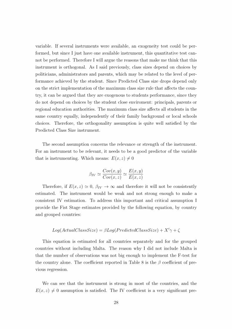
The second assumption concerns the relevance or strength of the instrument.

For an instrument to be relevant, it needs to be a good predictor of the variable

that is instrumenting. Which means: E(x, z) 6= 0

βIV 'Cov(x, y)

Cov(x, z)' E(x, y)

E(x, z)

Therefore, if E(x, z) ' 0, βIV → ∞ and therefore it will not be consistently

estimated. The instrument would be weak and not strong enough to make a

consistent IV estimation. To address this important and critical assumption I

provide the Fist Stage estimates provided by the following equation, by country

and grouped countries:

Log(ActualClassSize) = βLog(PredictedClassSize) +X ′γ + ζ

This equation is estimated for all countries separately and for the grouped

countries without including Malta. The reason why I did not include Malta is

that the number of observations was not big enough to implement the F-test for

the country alone. The coefficient reported in Table 8 is the β coefficient of pre-

vious regression.

We can see that the instrument is strong in most of the countries, and the

E(x, z) 6= 0 assumption is satisfied. The IV coefficient is a very significant pre-

28

dictor of English Class Size in 5 countries and in the grouped countries. Also,

the F-test that checks the validity of the complete First Stage IV model satisfies

the validity threshold since its p-value is lower than 0.05, meaning that, with a

probability higher than 0.95, we reject the null hypothesis that the model is not

statistically valid. Malta’s F-test cannot be performed since I do not have enough

observations to perform the test. Therefore I exclude Malta from the grouped

countries and from the complete IV model that will be estimated later.

IV First StageCountry Correlation Coefficient Prob > FBulgaria 0.2719 0.247 0.0000

(0.200)

Estonia 0.1448 0.360*** 0.0003(0.120)

Greece 0.2180 0.487*** 0.0000(0.153)

Spain 0.1277 0.311 0.0000(0.221)

France 0.4065 0.757*** 0.0000(0.205)

Malta 0.2720 -0.0160 –(0.168)

Portugal 0.4905 0.849*** 0.0000(0.0971)

Slovenia 0.0348 0.0831 0.0047(0.109)

Sweeden 0.2152 0.501** 0.0035(0.211)

All Countries 0.3766 0.459*** 0.0000(Malta excluded) (0.111)

Clustered Robust standard errors by school in parenthesesWheighted by students sampling probability

Table 8: Testing the Strength of the Instrument

4.2 English Class Size IV estimation

Table 9 provides the coefficient estimates by country and by pooled countries,

excluding Malta, of English Class size coefficients in logarithms using Ordinary

Least Squares (OLS) and Instrumental Variables (IV) two stage least squares

using the instrument Predicted Class size in logarithms. Again, I use population

29

weights by skill provided by the data for both estimations. Since the sample size

of some of the countries is small, I performed also a more robust IV estimation

method: limited information maximum likelihood (liml), which provides more

robust IV estimates in small samples. Since coefficient and errors do not present

any difference with respect to the standard two stage least squares, I exclude the

liml estimates for the sake of simplicity.

Mean Listening Mean Reading Mean WritingEnglish Class Size logs OLS IV Obs OLS IV Obs OLS IV Obs

Bulgaria 1.007** 0.410 281 0.594** -3.569* 316 0.797 -1.646 281(0.457) (1.992) (0.290) (2.067) (0.491) (1.856)

Estonia 0.461*** 0.531 666 0.164 0.565 655 0.329 1.258 656(0.159) (0.633) (0.200) (0.802) (0.375) (1.666)

Greece 0.101 0.0566 502 0.167 -0.00450 536 0.673*** 1.293 512(0.132) (0.328) (0.118) (0.674) (0.250) (0.885)

Spain 0.159 0.229 676 0.309*** 1.979* 688 0.469 1.345 664(0.101) (0.660) (0.116) (1.113) (0.301) (2.012)

France 0.290 -0.251 370 0.269 1.062** 362 1.231* 4.274** 347(0.189) (0.399) (0.180) (0.527) (0.643) (2.135)

Portugal 0.162 0.0591 702 -0.141 0.161 712 0.00185 -0.718 694(0.164) (0.353) (0.106) (0.355) (0.330) (0.864)

Slovenia 0.341** 4.810 550 0.0775 0.866 567 -0.156 -0.818 558(0.163) (7.370) (0.178) (2.777) (0.317) (6.420)

Sweden 0.421*** 0.0464 376 0.702*** 2.083** 359 1.388*** 4.456** 360(0.160) (0.973) (0.182) (0.857) (0.350) (2.213)

All Countries 0.191** -0.0293 4,158 0.280*** 1.002*** 4,195 0.655** 1.839** 4,072(Malta excluded ) (0.0972) (0.253) (0.0974) (0.355) (0.262) (0.847)

Robust standard errors in parentheses, *** p<0.01, ** p<0.05, * p<0.1Weighted by students sampling probability

Table 9: OLS and IV 2SLS Estimates

The OLS positive and significant coefficients of English Class size in loga-

rithms by country corroborate what previous studies like Woessmann (2005) had

found using European data: bigger classes perform better on average. The IV

coefficients provided by the two stage least squares using the ESLC data, give

us a surprising result. What previous researchers like Hoxby (2000), Woessmann

(2005) or Angrist and Lavy (1999) have obtained after using IV on class size effect

estimates was that class size coefficients turned negative or no longer significant.

That seems to be the case in the Listening skill, where, after using IV estimation,

the positive and very significant coefficient of English Class Size of Bulgaria, Es-

tonia, Slovenia, Sweden and the pooled European countries disappears, since the

IV coefficients are no longer statistically significantly different from zero. But a

different scenario appears with Reading and Writing skills estimates.

In the Reading skill estimates, for Bulgaria the class size coefficient turns very

30

negative and marginally significant, but for Spain, France, Sweden and All Coun-

tries estimates more than triple their size, and remain positive and significant. In

the case of France, Sweden and All Countries, coefficients are positive and signif-

icant at a 5% or even lower significance level.

In the Writing skill estimates, the same positive and significant pattern re-

mains in France, Sweden and All Countries estimates. Coefficients approximately

triplicate its size and the effect of English Class size remains positive, corrobo-

rating and exacerbating what the OLS coefficients have previously pointed out:

bigger classes perform better on average.

The fact that the coefficients become bigger, in absolute value, and remain

statistically significant after using IV, suggests that the endogeneity present in

the OLS estimates was due to measurement error, since this kind of endogeneity

problem creates a downward bias that make the OLS coefficient estimates smaller.

The Bulgaria negative class size marginally significant coefficient in Reading

implies what is expected: smaller classes perform better on average than big-

ger ones. This has a causal interpretation since this coefficient is obtained using

IV estimates. This seems natural since, the smaller the class, the smaller is the

student-teacher ratio, and therefore, the more time the teacher can dedicate to

each individual student.

However, the surprising positive causal result obtained in Spain, France, Swe-

den and All pooled countries, points to the opposite direction. In these countries

bigger classes perform better on average than smaller ones in Reading and Writ-

ing. What could be the explanation? One possibility could be that, since English

is a multi-skill ability and English lecture time is limited, teachers can make spe-

cial emphasis on one skill versus some other, and therefore allocate their limited

class time towards some particular English skills versus others. Therefore, if a

teacher has a bigger class, he/she could dedicate greater proportion of the class to

grammar, vocabulary and exercise correction rather than to speaking or listening

activities that could be more difficult to implement in larger classes. This focus on

grammar can make bigger classes more effective in English Writing and Reading

skills. Notice that this positive causal effect of bigger classes cannot be found

31

in any country in the Listening skill, a skill more related to practice and use of

the language teaching techniques, which require more individual and personalized

training and therefore, more teacher time per student.

And what is the global effect of this relative emphasis on some skills versus

some other of bigger classes? The effect of this Reading and Writing English skills

orientation could be improving the English level of the students in different ways

across countries. Remember that in Figure 1, when the Mean Tests results by

skill and country were ranked, Sweden performed the second best in all mean

evaluated skills and France the worst in all skills, but both countries present a

causal, very significant and positive effect of English class size in Reading and

Writing test scores.

This study provides causal English class size effects on English results, which

have important policy implications. Educational policy makers have always claimed

that class size reductions were the right policy to improve students’ results at all

levels and courses. A priori, it seems logic to assume that if classes are smaller,

the teacher can dedicate more time per student individually. However, previous

results clearly quantify the effect of English class sizes on performance in all eval-

uated English skills and they point towards the opposite direction in theoretical

skills. In particular, class size reductions will not be the right policy in Reading

and Writing skills. On the opposite, a better educational policy for English learn-

ing would be to increase classes for theoretical skills like Reading and Writing,

and to provide reduced classes for students to improve just their Listening and

Speaking skills.

5 Optimal English Class Size

Previous section has shown a positive causal effect of English Class size in loga-

rithms on Reading and Writing skills in France, Sweden and All Countries, ex-

cluding Malta. This positive class size means that bigger classes perform better

on average than smaller ones in the already mentioned skills. But what does big

actually mean in terms of class size? The variable English Class size, that I used

in OLS and IV estimation is composed of 19,331 observations that vary from 1 to

43, it has a mean of 20.19 and a standard deviation of aproximately 6 students.

32

The English Class size OLS estimates in the original Multivariate specification

was positive and significant. The logarithm functional form gives us the coeffi-

cient estimates of part 3 which are bigger than the Class Size coefficient in levels,

therefore suggesting that a logarithm functional form is more appropriate to cap-

ture the effect of class size on English skills. The positive effect obtained in the

logarithm specification was maintained using IV estimation methods as has been

shown in the previous section in Reading and Writing skills.

However it would be interesting to know whether this more curved functional

form provided by logarithms is actually hiding an optimal maximum class size that

makes bigger classes better than smaller ones up a point, and the moment that

this class size limit is surpassed, bigger classes do not necessarily perform better

on average than smaller ones. To address this possibility I vary the multivariate

original specification by replacing the English class size logarithm functional form

by the following:

α(log(EngClassSize)) + β(log(EngClassSize))2

which gives nonsignificant α nor β, therefore it suggests that this functional

form is not appropriate.

The second modification I implement consists on altering the multivariate

original specification by replacing the English class size functional form by the

following:

α(EngClassSize) + β(EngClassSize)2

which provides the coefficient estimates given by Table 10, which are highly

statistically significant and robust to School Fixed Effects specification that, as

explained previously, removes the between-school sorting bias.

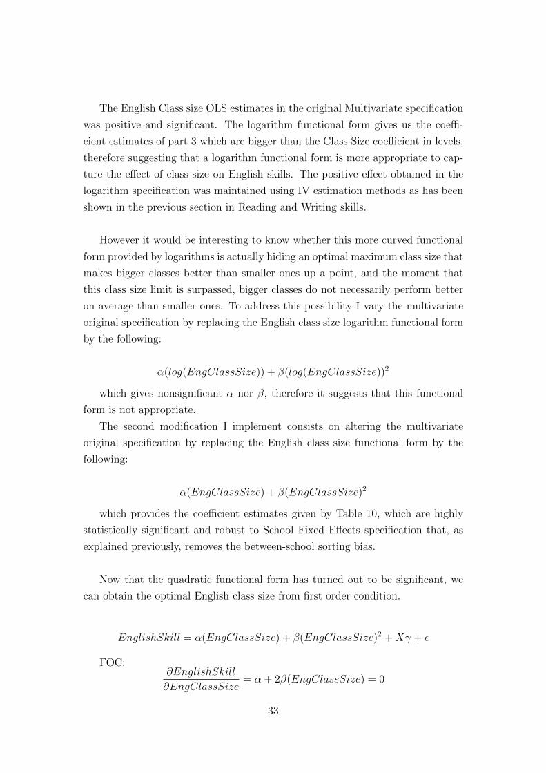
Now that the quadratic functional form has turned out to be significant, we

can obtain the optimal English class size from first order condition.

EnglishSkill = α(EngClassSize) + β(EngClassSize)2 +Xγ + ε

FOC:∂EnglishSkill

∂EngClassSize= α + 2β(EngClassSize) = 0

33

(1) (2) (3)School Fixed Effects Mean Listening Mean Reading Mean Writing

English Class Size 0.0403*** 0.0438*** 0.115***(0.0113) (0.0104) (0.0268)

English Class Size Squared -0.000652** -0.000624*** -0.00177***(0.000266) (0.000224) (0.000634)

Observations 10,486 10,573 10,372R-squared 0.647 0.596 0.623Clustered robust standard errors by school, *** p<0.01, ** p<0.05, * p<0.1

Weighted by students sampling probability

Table 10: Optimal Class Size

Therefore the optimal English class size is given by

EngClassSize∗ = − α

2β

Substituting the obtained estimation results for α and β we obtain the optimal

English class size.

EngClassSize∗List = 30.9

EngClassSize∗Read = 35.096

EngClassSize∗Writ = 32.486

Figure 4 plots the English class size under the Logarithm initial especification

of Listening and Reading (which had a very similar coefficient) and the functional

forms provided by the quadratic function used in this section: Table 10 estimates.

Therefore, the optimal class size of Reading and Writing skills are bigger than

the ones given by the strict implementation of the Maximum class size rules in

Europe, which varied from 24 to 30.

34

6 Conclusion

This paper studies the main determinants of English performance at the end of

compulsory education by using the European Survey of Language Competences

(ESLC) that was carried out in 2011. The significant variability of English skill

test results across countries, which were significantly illustrated by the descrip-

tive results of Section 2, motivates the first part of this study, where we wanted

to explore which factors were behind them. Therefore, we estimated the main

determinants of English proficiency at the end of compulsory education by using

the contextual information provided by the Student Questionnaire and National

Information. The standard educational production function commonly used in

the Education literature was improved in order to take into account factors that

affect languages specifically, such as family language controls. By using this im-

proved function, we have been able to obtain the main determinants of English

performance. To address the accuracy of the estimation, robustness checks are

also reported.

The second part of my analysis focuses on a very significant determinant that

was found in the education production function: the positive and significant ef-

fect that English class size has on English skills, which implies that bigger English

classes perform better on average than smaller ones. This result is in line with

other least squares positive class size effects found using European data such as

Woesmann (2005).

When educational politicians wonder how to improve the educational perfor-

mance of students, they often suggest reducing class sizes: if students are taught

in smaller classes, increased individual attention may lead to a better learning,

or at least that is what has been believed so far. Finance ministers, by contrast,

caution that class-size reductions are a very expensive policy. The second part of

my study addresses precisely that assumption: whether smaller English classes are

better in terms of performance. Least square estimates points contrary to what

has been believed: the positive and significant English class size coefficients in

all evaluated skills indicate that bigger classes perform better than smaller ones.

However, least squares coefficients are very likely to be biased. To address this

important concern, and taking into account that 9 out of 13 countries in the ESLC

sample have maximum class size regulations, I build an instrument in line with

35

Angrist and Lavy (1999) Maimonides’ rule. Performing Instrumental Variables

estimation on the three ESLC evaluated skills gives us a surprising result: positive

class size effects are obtained in France, Sweden and pooled European countries

in Reading and Writing skills. Contrary to what has been believed so far, big-

ger classes do not necessarily make students perform worse in all cognitive skills

and moreover, it made them perform better in Reading and Writing English skills.

What could be the explanation? One possibility could be that, since English

is a multi-skill ability, and since English lecture time is limited, teachers can make

special emphasis on one skill versus some other, and therefore, they allocate their

limited class time towards some particular English skills versus others. There-

fore, if a teacher has a bigger class, she could dedicate greater part of the class

to grammar, vocabulary and exercise correction rather than speaking or listen-

ing, activities that could be more difficult to implement in greater classes. This

focus on grammar can make bigger classes more effective in English Writing and

Reading skills. Notice that this positive and causal result is not obtained for any

country in Listening, a skill that is more related to practice and which requires

more individual attention, requiring more teacher time per student.

To complete this study, I provide the optimal class size in the three skills.

Reading and Writing English skills present an optimal class size of 35 and 33

respectively, which are bigger than the ones implemented by the maximum class

size regulations across Europe, that vary from 24 to 30. This study provides

causal English class size effects on English outcomes, which have important pol-

icy implications. In particular, class size reduction will not be the right policy in

Reading and Writing English skills, as my results have shown. On the opposite, a

better option would be to increase classes up to the optimal level for Reading and

Writing skills, and to provide reduced classes for students to improve just their

Listening and Speaking skills.

For further studies, it will be necessary to accomplish the fact that English is

a multi-skill ability, and therefore relative emphasis that a teacher does on some

skills versus others could create students that are very good at some skills such as

Reading and Writing skills, but are totally unable to speak or understand spoken

English.

36

7 References

Joshua D. Angrist and Victor Lavy (1999): ”Using Maimonides’ rule to estimate

the effect of Class Size on Scholastic Achievement”, The Quarterly Journal of

Economics 114 (2): 533-575.

Jan Bietenbeck (2014): ”Teaching Practices and cognitive Skills”, Labour Eco-

nomics, Volume 30, October 2014, Pages 143–153.

Eric A. Hanushek and Dennis D. Kimko (2000): ”Schooling, Labor-Force Qual-

ity, and the Growth of Nations”, American Economic Review, Vol. 90 (5).

Erik A. Hanushek, Stephen Machin and Ludger Woßmann (2011):”Handbook

of the Economics of Education Volume 3”, Elsevier 2011, North Holland.

Eric A. Hanushek and Ludger Woßmann (2012): ”The Economic Benefit of

Educational Reform in the European Union”, CESifo Economic Studies, Vol 58,

Oxford University Press.

Caroline M. Hoxby (2000): ”The effects of class size on student achievement:

New evidence from population variation”, The Quarterly Journal of Economics

115 (4): 1239-1285.

Victor Lavy (2011): ”What Makes an Effective Teacher? Quasi-Experimental

Evidence”, NBER Working Paper No. 16885.

Elke Ludemann, Gabriela Schutz, Martin R. West and Ludger Woßmann

(2005): ”School Accountability, Autonomy, Choice and the Level of Student

achievement: International evidence from PISA 2003”, Education Working Pa-

per N 13.

Elke Ludemann, Gabriela Scxhutz, Martin R. West and Ludger Woßmann

(2007): ”School Accountability, Autonomy and Choice around the World”, Ed-

ward Elgar.

Gabriela Schutz, Martin R. West and Ludger Woßmann (2007): ”School Ac-

37

countability, Autonomy, Choice and the Equity of Student achievement: Interna-

tional evidence from PISA 2003”, Education Working Paper N 14.

Martin R. West and Ludger Woßmann (2003): ”Which schools systems sort

weaker students into smaller classes? International evidence”, CESifo Working

Paper 1054.

Ludger Woßmann (2005): ”The Educational production in Europe”, Economic

Policy Vol 20 (43): 445–504.

38

Mean Listening Mean Reading Mean Writing(1) (2) (3) (4) (5) (6)

STUDENT CHARACTERISTICSAge -0.14*** -0.11*** -0.09*** -0.12*** -0.19** -0.20**

(0.03) (0.03) (0.03) (0.03) (0.08) (0.10)Female 0.02 0.02 0.01 0.01 0.47*** 0.47***

(0.026) (0.027) (0.031) (0.032) (0.08) (0.08)Repetition -0.18*** -0.19*** -0.36*** -0.29*** -1.27*** -1.24***

(0.057) (0.06) (0.06) (0.06) (0.13) (0.14)Immigrant 0.22*** 0.22*** 0.10 0.11 0.19 0.20

(0.0819) (0.0809) (0.0811) (0.0806) (0.223) (0.224)FAMILY BACKGROUNDBooks 26-100 0.016 0.02 0.09** 0.08** 0.41*** 0.41***

(0.0443) (0.0442) (0.0383) (0.0381) (0.134) (0.134)Books 101-200 0.15*** 0.16*** 0.25*** 0.25*** 0.67*** 0.67***

(0.0416) (0.0415) (0.0441) (0.0437) (0.127) (0.127)Books>200 0.20*** 0.21*** 0.34*** 0.33*** 0.76*** 0.76***

(0.0492) (0.0497) (0.0535) (0.0530) (0.140) (0.141)ESCS index 0.14*** 0.13*** 0.15*** 0.14*** 0.25*** 0.25***

(0.0253) (0.0255) (0.0288) (0.0293) (0.0836) (0.0845)Father University 0.08* 0.09** 0.09* 0.09** 0.28** 0.29**

(0.0397) (0.0400) (0.0474) (0.0473) (0.118) (0.119)Mother University 0.13*** 0.12*** 0.11** 0.10** 0.34*** 0.34***

(0.0425) (0.0420) (0.0471) (0.0471) (0.104) (0.104)White Collar Father 0.02 0.03 0.03 0.03 -0.13 -0.12

(0.0387) (0.0383) (0.0473) (0.0470) (0.117) (0.116)White Collar Mother 0.16*** 0.16*** 0.23*** 0.22*** 0.62*** 0.62***

(0.0464) (0.0469) (0.0479) (0.0482) (0.133) (0.133)Blue Collar Father -0.10*** -0.11*** -0.12*** -0.14*** -0.43*** -0.43***

(0.0390) (0.0389) (0.0401) (0.0402) (0.132) (0.132)Pink Collar Mother 0.09*** 0.09*** 0.09** 0.09** 0.51*** 0.51***

(0.0335) (0.0333) (0.0446) (0.0449) (0.125) (0.126)Father English Well 0.16*** 0.14*** 0.16*** 0.15*** 0.48*** 0.47***

(0.0335) (0.0342) (0.0342) (0.0343) (0.0980) (0.100)Mother English Well 0.039 0.02 0.04 0.03 0.12 0.11

(0.0313) (0.0313) (0.0397) (0.0392) (0.0959) (0.0974)English use at home 0.41*** 0.41*** 0.35*** 0.35*** 0.98*** 0.98***

(0.0434) (0.0431) (0.0532) (0.0529) (0.136) (0.136)Early Onset at home 0.24*** 0.23*** 0.21** 0.20** 0.45** 0.42**

(0.0724) (0.0736) (0.0824) (0.0836) (0.183) (0.185)SCHOOL INFORMATIONEnglish Hours per Week 0.08*** 0.09*** 0.10*** 0.10*** 0.26*** 0.26***

(0.0257) (0.0254) (0.0302) (0.0302) (0.0669) (0.0669)Years English School >5 years 0.03*** 0.03*** 0.05*** 0.05*** 0.08*** 0.08***

(0.00618) (0.00611) (0.00655) (0.00661) (0.0204) (0.0201)Early Onset at School<5 years 0.17*** 0.20*** 0.18*** 0.19*** 0.50*** 0.51***

(0.0587) (0.0593) (0.0596) (0.0593) (0.132) (0.133)Number of Foreign Languages 0.12*** 0.12*** 0.10*** 0.10*** 0.21*** 0.20***

(0.0237) (0.0237) (0.0274) (0.0271) (0.0661) (0.0660)Ancient Languages 0.8 0.10* 0.13** 0.16*** 0.39*** 0.39***

(0.0533) (0.0550) (0.0581) (0.0596) (0.146) (0.149)English Class Size logarithms 0.15*** 0.18*** 0.20*** 0.24*** 0.75*** 0.76***Fam.Language Controls yes no yes no yes noCountry Controls no yes no yes no yesObservations 10,221 10,221 10,350 10,350 10,144 10,144R-squared 0.502 0.508 0.442 0.448 0.440 0.441

Clustered robust standard errors by school in parentheses, *** p<0.01, ** p<0.05, * p<0.1Weighted by students sampling probability

Table 11: Family Language Controls and Country Controls

39

Student TypeCountry (1) (2) (3) TotalBelgium fr 432 435 438 1,305Bulgaria 343 322 318 983Estonia 439 445 438 1,322Greece 343 317 356 1,016Spain 450 442 452 1,344France 341 312 315 968Croatia 419 454 460 1,333Malta 293 294 286 873Netherlands 402 407 422 1,231Poland 440 428 448 1,316Portugal 458 441 445 1,344Sweden 363 340 343 1,046Slovenia 373 364 395 1,132Total 5,096 5,001 5,116 15,213

Table 12: Student Type by Country, observations with missing values eliminated

Correlation Variable Observations Mean Std. Dev. Min MaxStudent 0.82 Mean Listening 5096 0.57 1.19 -3.725 5.367Type 1 Mean Reading 5096 0.46 1.24 -3.779 5.692Student 0.79 Mean Listening 5001 0.61 1.23 -4.57 5.72Type 2 Mean Writing 5001 -1.08 2.95 -11.61 9.527Student 0.81 Mean Reading 5116 0.45 1.24 -2.71 6.02Type 3 Mean Writing 5116 -1.04 2.92 -12.23 10.92

Weighted by students sampling probability

Table 13: Mean Results and Correlations once missing values are eliminated

40

Student Type 1 Student Type 2 Student Type 3VARIABLES Mean List Mean Read Mean List Mean Writ Mean Read Mean Writ

(1) (2) (3) (4) (5) (6)STUDENTBACKGROUNDAge -0.15*** -0.07** -0.12*** -0.08 -0.12*** -0.29***

(0.0333) (0.0323) (0.0377) (0.106) (0.0407) (0.109)Female -0.04 -0.04 0.07* 0.59*** 0.05 0.38***

(0.0389) (0.0426) (0.0375) (0.120) (0.0423) (0.129)Repetition -0.11 -0.34*** -0.25*** -1.65*** -0.32*** -0.88***

(0.0734) (0.0717) (0.0699) (0.209) (0.0705) (0.205)Immigrant 0.27** 0.20 0.18 0.46 0.041 0.06

(0.114) (0.125) (0.122) (0.292) (0.115) (0.275)FAMILYBACKGROUNDBooks 26-100 0.03 0.09 -0.02 0.28* 0.09* 0.49***

(0.0513) (0.0581) (0.0669) (0.151) (0.0510) (0.188)Books 101-200 0.14** 0.24*** 0.16*** 0.49*** 0.28*** 0.82***

(0.0604) (0.0685) (0.0568) (0.167) (0.0568) (0.192)Books>200 0.20*** 0.3*** 0.18*** 0.59*** 0.37*** 0.87***

(0.0602) (0.0709) (0.0682) (0.184) (0.0724) (0.189)ESCS index 0.19*** 0.19*** 0.06* 0.34** 0.10** 0.19*

(0.0366) (0.0384) (0.0361) (0.140) (0.0391) (0.114)Father University 0.06 0.08 0.12** 0.31** 0.11 0.23

(0.0587) (0.0665) (0.0518) (0.159) (0.0657) (0.176)Mother University 0.06 0.11 0.17*** 0.30* 0.14** 0.41**

(0.0610) (0.0704) (0.0589) (0.165) (0.0609) (0.161)White Collar Father 0.07 0.06 -0.03 -0.38** 0.03 0.16

(0.0592) (0.0708) (0.0513) (0.176) (0.0701) (0.164)White Collar Mother 0.14** 0.24*** 0.22*** 0.59*** 0.19*** 0.53**

(0.0694) (0.0682) (0.0559) (0.160) (0.0679) (0.216)Blue Collar Father -0.06 -0.10* -0.14** -0.62*** -0.12* -0.21

(0.0487) (0.0539) (0.0566) (0.185) (0.0633) (0.176)Pink Collar Mother 0.08 0.07 0.12*** 0.41*** 0.10* 0.57***

(0.0505) (0.0604) (0.0453) (0.145) (0.0583) (0.220)Father English Well 0.13*** 0.12** 0.20*** 0.45*** 0.19*** 0.54***

(0.0443) (0.0545) (0.0566) (0.154) (0.0471) (0.133)Mother English Well 0.06 0.003 0.02 0.0001 0.12** 0.23*

(0.0477) (0.0557) (0.0502) (0.135) (0.0505) (0.126)English use at home 0.34*** 0.29*** 0.47*** 1.06*** 0.36*** 0.88***

(0.0555) (0.0683) (0.0743) (0.157) (0.0818) (0.178)Early Onset at home 0.26*** 0.21* 0.21* 0.57** 0.27** 0.26

(0.0933) (0.110) (0.125) (0.230) (0.128) (0.252)SCHOOLINFORMATIONEnglish Hours per Week 0.07** 0.11*** 0.10*** 0.25*** 0.12** 0.28***

(0.0295) (0.0288) (0.0319) (0.0696) (0.0469) (0.0972)Years English School >5 years 0.03*** 0.04*** 0.02** 0.07** 0.06*** 0.10***

(0.00856) (0.00917) (0.00874) (0.0280) (0.00979) (0.0276)Early Onset at School<5 years 0.09 0.14* 0.26*** 0.47** 0.19*** 0.58***

(0.0688) (0.0786) (0.0762) (0.199) (0.0701) (0.164)Number of Foreign Languages 0.07** 0.09*** 0.15*** 0.16* 0.12*** 0.25***

(0.0343) (0.0350) (0.0300) (0.0875) (0.0349) (0.0909)Ancient Languages 0.06 0.13* 0.07 0.53*** 0.14* 0.27

(0.0668) (0.0718) (0.0675) (0.196) (0.0751) (0.205)English Class Size logarithms 0.11* 0.19*** 0.19*** 0.92*** 0.18** 0.64***

(0.0577) (0.0645) (0.0729) (0.239) (0.0791) (0.182)INSTITUTIONALINFORMATIONGDP ppa 2010 per capita -0.06** -0.05** -0.08*** -0.21*** -0.08*** -0.15**

(0.0235) (0.0247) (0.0250) (0.0593) (0.0273) (0.0635)Educational Expenditure 2010 0.15** 0.12 0.17** 0.69*** 0.16** 0.55***

(0.0678) (0.0718) (0.0699) (0.160) (0.0775) (0.167)TV English not dubbed 0.15 0.31*** 0.13 0.59** 0.04 0.36

(0.110) (0.118) (0.127) (0.283) (0.135) (0.322)Population 2011 -0.11*** -0.04** -0.12*** -0.18*** -0.08*** -0.21***

(0.0172) (0.0190) (0.0182) (0.0451) (0.0205) (0.0481)Multilingual Region 0.19 0.14 0.34** 0.45 0.001 0.75*

(0.146) (0.182) (0.139) (0.543) (0.173) (0.383)External Exit Exams -0.13 -0.38*** -0.10 -0.62*** -0.30*** -0.72***

(0.0821) (0.0948) (0.102) (0.226) (0.104) (0.260)Observations 5,096 5,096 5,001 5,001 5,116 5,116R-squared 0.504 0.437 0.503 0.463 0.451 0.426

Clustered robust standard errors by school in parentheses, *** p<0.01, ** p<0.05, * p<0.1

Table 14: Same Student Regression Results41

Country Obs Obs with CohortSize Obs with any missingBulgaria 1,563 671 475Estonia 1,645 1,244 990Greece 1,583 1,180 784Spain 1,719 1,274 1,031France 1,503 812 546Malta 1,177 431 307Portugal 1,580 1,221 1,060Slovenia 1,586 1,156 841Sweeden 1,513 795 549All Countries 12,692 8,353 6,276(Malta excluded )

Table 15: Observations available for IV estimation

Figure 4: Class Size Functional Forms

42

A Appendix

The following appendix provides more detailed information of the variables used.

Information provided by the institutional/country variables was obtained from

Eurostat, from Eurydice, a European network on education systems and policy

and from the ESLC. The variables that come from Eurostat information are GDP

per capita in purchasing power parity of 2010 in prices from 2005, Educational

Expenditure on secondary education per student in 2010 in prices from 2005, and

country Population in January 2011 expressed in tens of million (for Belgium re-

gional information from Eurostat was needed to obtain the Wallonia population).

The information that comes from Eurydice is: the External Exit Exams (if

the students have to perform an external exit exam to get their lower secondary

education degree), which according to Eurydice it is the case for Malta, France,

Portugal, Netherlands, Poland and Estonia; and the grouping criteria necessary

to compute the repetition variable. Eurydice also provided information about the

school grouping criteria of students at the beginning of primary education, which

allowed me to obtain an accurate measure of the Repetition variables. Most of

the European countries have as grouping criteria the natural year: therefore all

students born in the same year are grouped in the same grade. However, some

countries in my sample do not grouped students by the criteria of having the

same age by January 1st, as it was the case for Netherlands and Estonia, which

groups by same age in October 1st; and Croatia, which date isMarch 1st.Family

Language controls were also obtained from Eurydice.

The rest of the Institutional variables were obtained by using the ESLC data

which provide me information regarding about Multilingual regions, and informa-

tion regarding the media, which was used to build the TV not dubbed variable.

The Student Variables come from the Student Questionnaire (SQ). The Age

reports the exact age at the beginning of February 2011, since that was the exact

month of the study. To compute it, I use the date of birth provided by the stu-

dents.Parents occupation indicators White, Blue, Pink Collar come from a variable

that reports the exact occupation of the parents, according to international ISCO

index. In order to use it in my study, I transformed into collar indicators. The

43

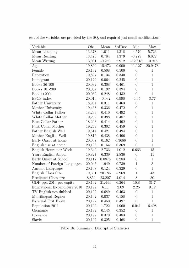
rest of the variables are provided by the SQ, and required just small modifications.

Variable Obs Mean StdDev Min MaxMean Listening 13,378 1.011 1.318 -4.570 5.723Mean Reading 13,475 0.784 1.379 -3.779 6.022Mean Writing 13,031 -0.259 2.912 -12.818 10.916Age 19,869 15.472 0.900 11.127 20.9473Female 20,132 0.508 0.500 0 1Repetition 19,897 0.134 0.340 0 1Immigrant 20,129 0.064 0.245 0 1Books 26-100 20,032 0.308 0.461 0 1Books 101-200 20,032 0.192 0.394 0 1Books>200 20,032 0.248 0.432 0 1ESCS index 20,010 -0.032 0.998 -4.65 3.77Father University 18,934 0.311 0.463 0 1Mother University 19,438 0.336 0.472 0 1White Collar Father 18,293 0.410 0.492 0 1White Collar Mother 19,269 0.388 0.487 0 1Blue Collar Father 18,293 0.414 0.492 0 1Pink Collar Mother 19,269 0.302 0.459 0 1Father English Well 19,614 0.421 0.494 0 1Mother English Well 19,816 0.438 0.496 0 1Early Onset at home 20,007 0.162 0.3686 0 1English use at home 20,103 0.154 0.369 0 1English Hours per Week 19,642 2.733 1.012 0.666 15Years English School 19,827 6.339 2.836 0 11Early Onset at School 20,117 0.0875 0.283 0 1Number of Foreign Languages 20,045 1.949 0.739 1 8Ancient Languages 20,108 0.124 0.329 0 1English Class Size 19,331 20.186 5.969 1 43Predicted Class size 8,859 23.207 4.014 8 30GDP ppa 2010 per capita 20,192 21.444 6.264 10.8 31.7Educational Expenditure 2010 20,192 6.11 2.09 2.26 9.12TV English not dubbed 20,192 0.689 0.463 0 1Multilingual Region 20,192 0.037 0.188 0 1External Exit Exam 20,192 0.450 0.497 0 1Population 2011 20,192 1.722 1.960 0.041 6.498Germanic 20,192 0.145 0.352 0 1Romance 20,192 0.370 0.483 0 1Slavic 20,192 0.325 0.468 0 1

Table 16: Summary: Descriptive Statistics

44

MASTER’S THESIS CEMFI

0801 Paula Inés Papp: “Bank lending in developing countries: The effects of foreign

banks”.

0802 Liliana Bara: “Money demand and adoption of financial technologies: An analysis with household data”.

0803 J. David Fernández Fernández: “Elección de cartera de los hogares españoles: El papel de la vivienda y los costes de participación”.

0804 Máximo Ferrando Ortí: “Expropriation risk and corporate debt pricing: the case of leveraged buyouts”.

0805 Roberto Ramos: “Do IMF Programmes stabilize the Economy?”.

0806 Francisco Javier Montenegro: “Distorsiones de Basilea II en un contexto multifactorial”.

0807 Clara Ruiz Prada: “Do we really want to know? Private incentives and the social value of information”.

0808 Jose Antonio Espin: “The “bird in the hand” is not a fallacy: A model of dividends based on hidden savings”.

0901 Víctor Capdevila Cascante: “On the relationship between risk and expected return in the Spanish stock market”.

0902 Lola Morales: “Mean-variance efficiency tests with conditioning information: A comparison”.

0903 Cristina Soria Ruiz-Ogarrio: “La elasticidad micro y macro de la oferta laboral familiar: Evidencia para España”.

0904 Carla Zambrano Barbery: “Determinants for out-migration of foreign-born in Spain”.

0905 Álvaro de Santos Moreno: “Stock lending, short selling and market returns: The Spanish market”.

0906 Olivia Peraita: “Assessing the impact of macroeconomic cycles on losses of CDO tranches”.

0907 Iván A. Kataryniuk Di Costanzo: “A behavioral explanation for the IPO puzzles”.

1001 Oriol Carreras: “Banks in a dynamic general equilibrium model”.

1002 Santiago Pereda-Fernández: “Quantile regression discontinuity: Estimating the effect of class size on scholastic achievement”.

1003 Ruxandra Ciupagea: “Competition and “blinders”: A duopoly model of information provision”.

1004 Rebeca Anguren: “Credit cycles: Evidence based on a non-linear model for developed countries”.

1005 Alba Diz: “The dynamics of body fat and wages”. 1101 Daniela Scidá: “The dynamics of trust: Adjustment in individual trust levels to

changes in social environment”. 1102 Catalina Campillo: “Female labor force participation and mortgage debt”. 1103 Florina Raluca Silaghi: “Immigration and peer effects: Evidence from primary

education in Spain”. 1104 Jan-Christoph Bietenbeck: “Teaching practices and student achievement:

Evidence from TIMSS”.

1105 Andrés Gago: “Reciprocity: Is it outcomes or intentions? A laboratory

experiment”. 1201 Rocío Madera Holgado: “Dual labor markets and productivity”. 1202 Lucas Gortazar: “Broadcasting rights in football leagues and TV competition”. 1203 Mª. Elena Álvarez Corral: “Gender differences in labor market performance:

Evidence from Spanish notaries”. 1204 José Alonso Olmedo: “A political economy approach to banking regulation”. 1301 Joaquín García-Cabo Herrero: “Unemployment and productivity over the

business cycle: Evidence from OECD countries”. 1302 Luis Díez Catalán: “Collective bargaining and unemployment during the Great

Recession: Evidence from Spain”. 1303 Cecilia Dassatti Camors: “Macroprudential and monetary policy: Loan-level

evidence from reserve requirements”. 1304 Juan Carvajal: “Choosing to invest in human capital through adult education”. 1401 Haritz Garro: “Desire to win and public information in majority rule elections”. 1402 Álvaro Martín Herrero: “Credit and liquidity risk in sovereign bonds”. 1403 José Carreño: “Housing bubbles, doubts and learning”. 1404 Ester Núñez de Miguel: “Excuse me, do you speak English? An international

evaluation”.