THE ECONOMIC IMPACTS OF HELP TO BUY*

Felipe Carozzi

London School of Economics & Centre for Economic Performance

and

Christian A. L. Hilber

London School of Economics & Centre for Economic Performance

and

Xiaolun Yu

London School of Economics

This Version: September 24, 2019

* We thank Paul Cheshire, Steve Gibbons, Ingrid Gould Ellen and Henry Overman and conference/seminar

participants at the Penn-Oxford Symposium on Housing Affordability in the Advanced Economies, the European

meeting of the Urban Economics Association, the London School of Economics and University College London

for helpful comments and suggestions. We thank Hans Koster and Ted Pinchbeck who provided code helping us

to merge Land Registry and Energy Performance Certificate data. Financial support from LSE Advancement is

gratefully acknowledged. All errors are the sole responsibility of the authors. Address correspondence to: Felipe

Carozzi, London School of Economics, Department of Geography and Environment, Houghton Street, London

WC2A 2AE, United Kingdom. Phone: +44-20-7107-5016. E-mail: f.carozzi@lse.ac.uk.

THE ECONOMIC IMPACTS OF HELP TO BUY

Abstract

The British government introduced its new flagship housing policy—Help to Buy (HtB)—in

2013. The policy aims to help households, especially first-time buyers, to overcome their credit

and liquidity constraints, stimulate housing construction and increase housing affordability. To

explore the economic impacts of HtB, we exploit a difference-in-discontinuities design, taking

advantage of spatial discontinuities in the scheme that emerge at the Greater London Authority

(GLA) boundary and the English/Welsh border post implementation. We find that HtB

substantially increased house prices and had no discernible effect on construction volumes or

aggregate private mortgage lending in the GLA, where housing supply is subject to severe long-

run constraints and housing is already extremely unaffordable. HtB did increase construction

numbers without affecting prices near the English/Welsh border, an area with less binding

supply constraints and comparably affordable housing. HtB also led to bunching of newly built

units below the price threshold, building of smaller new units and an improvement in the

financial performance of developers. We conclude that HtB may be an ineffective policy in

already unaffordable areas.

JEL classification: G28, H24, H81, R21, R28, R31, R38.

Keywords: Help to buy, house prices, construction, housing supply, land use regulation.

1

1. Introduction

House prices in the UK have risen more in real terms between 1970 and 2015 than in any other

OECD country.1 During this period, housing has become increasingly unaffordable in large

parts of the country, especially in London and the South East of England. This remarkable

increase in house prices—especially relative to earnings—has led to a stark reduction in the

number of first-time buyers. Homeownership attainment amongst those in their 20s decreased

from 50% in 1993 to 20% in 2013. At the aggregate level, the homeownership rate in the UK

decreased from nearly 70% in 2002 to about 61% in 2017.2

The worsening affordability crisis ultimately led the British government to announce a new

flagship housing policy in 2013: Help to Buy (HtB). The policy was announced during the

Budget Speech in March 2013 and was implemented in April of that same year. The program

was initially only implemented in England, but Welsh and Scottish versions were put in place

within a year. At time of implementation, HtB consisted of four different schemes: Equity

Loans, Mortgage Guarantees, Shared Ownership, and Individual Savings Accounts (ISA).3 All

four schemes aim to help credit constrained households to buy a property.

In this paper, we set out to explore the causal impact of HtB on housing construction, house

prices, the size of newly constructed units and the performance of residential developers. To do

so, we focus on the Equity Loan scheme (ELS), which provides an equity loan for up to 20%

of the housing unit’s value (or 40% within the Greater London Authority, GLA) to buyers of

new build properties. The ELS is by far the most salient and popular of the four schemes and

the one requiring the biggest budget. The ELS is often referred to simply as “Help to Buy” and

henceforth, unless we note otherwise, when we refer to HtB we mean the ELS.

The ELS expands housing credit and thus increases demand for housing. To explore how such

a positive demand shock in the housing market affects construction and prices, we develop a

simple theoretical framework with heterogeneous households and credit constraints. Our model

predicts that the impact of the policy depends crucially on the supply price elasticity of housing.

In a setting with elastic supply, HtB can be expected to mainly stimulate construction numbers

as intended by the policy. However, when supply is price inelastic (i.e., regulatory constraints

or physical barriers to residential development impede a supply-response), the effect of the

policy may be mainly to increase house prices, with the unintended consequence of making

housing less rather than more affordable.

In our empirical analysis, we exploit spatial discontinuities in the generosity of the ELS and the

timing of implementation (pre vs. post) to identify the causal impact of HtB on housing

construction and house prices.

1 Based on the OECD Economic Outlook Database (last accessed: 29 April 2019). House prices in the UK

appreciated by 337 percent in real terms during this period. 2 The data is derived from the Survey of English Housing from 1993/4 to 2007/8 and from the English Housing

Survey from 2008/9. For an in-depth analysis of the intergenerational links in homeownership attainment and its

role for social mobility see Blanden and Machin (2017). 3 The Mortgage Guarantees scheme ceased at the end of 2016. The HtB-ISA closes for new entrants in November

2019 and any bonus must be claimed by 2030. In April 2017, the British government introduced a new Lifetime

ISA scheme. In contrast to HtB ISA, it is only open to individuals aged 18-39 and the money saved can also be

used to fund a pension.

2

We implement a difference-in-discontinuity design to compare changes in house prices and

construction activities across jurisdictional boundaries. We separately analyze properties sold

on either side of the GLA boundary and on either side of the English/Welsh border. In both

cases we only consider housing purchases close to the respective boundaries. As pointed out

above, in Wales the scheme was put in place later and it only applied to a subset of the properties

that were eligible in England. Likewise, the London scheme that was implemented in 2016,

offered larger government equity loans (as a share of house values) for dwellings inside the

GLA compared to those available for purchase outside the GLA. Our main estimates exploit

these spatial discontinuities to study the effect of the ELS on house prices and construction

activity. We also use this design to study the impact of the scheme on the size of newly

constructed units and on total private mortgage lending.

We focus on the GLA boundary and the English/Welsh border for two reasons. First, our

research design requires spatial discontinuities in the scheme’s conditions, which can be found

in these boundaries. Second, the two areas differ starkly in their regulatory land use

restrictiveness and in barriers to physical development: While the GLA is the most supply

constrained and the least affordable area in the UK – and arguably one of the most supply

constrained areas in the world – housing supply is comparably responsive to demand shocks

near the English/Welsh border.4

Consistent with our theoretical predictions, we find that differences in the intensity of the HtB-

treatment have heterogeneous effects depending on local supply restrictions and the local price

elasticity of housing supply. In the GLA, where the supply elasticity is low, the introduction of

the more generous London version of the ELS led to a significant increase in prices for new

build units of roughly 6%. However, it had no appreciable effect on construction activity or on

aggregate private mortgage lending. Conversely, in the relatively high supply elasticity areas

around the English/Welsh border, where only a small fraction of land is developed and

developable land is readily available, we find a significant effect on construction activity and

no effect on prices. The introduction of the more generous HtB-price threshold on the English

side of the border increased the likelihood of a new build sale by about 6 to 7% (compared to

the Welsh side of the border). Moreover, it decreased the size of newly constructed units on the

English side of the border by nearly 7%. Consistent with this, a bunching analysis reveals that

the English ELS led to significant bunching of properties right below the price threshold,

shifting construction away from larger properties above the threshold towards smaller units.

We also provide evidence indicating that the scheme caused an increase in developers’ financial

performance, leading to larger revenues, gross profits and net profits.

Collectively, these results suggest that the effects of HtB largely depend on local supply

conditions. We find that the scheme fails to trigger more construction activity, but instead

causes house prices to increase inside the GLA, precisely the region that is most strongly

adversely affected by the ‘affordability crisis’. This has distributional implications. Our

findings indicate that the main beneficiaries of HtB in already unaffordable areas may be

developers and (typically well-off) landowners rather than struggling first-time buyers.

4 We provide supporting evidence for this proposition in Section 3.2.

3

Our paper relates to the literature that looks at the effects of credit conditions and demand

subsidies on housing markets. Previous research in this vast literature has mainly focused on

the effect of credit supply on housing prices (see Stein 1995, Ortalo-Magne and Rady 2006,

Mian et al. 2009, Duca et al. 2011, Favara and Imbs 2015). These and other studies provide

theoretical and empirical credence to the notion that expansions in credit supply lead to higher

prices, especially in areas with tight planning conditions. Other studies have explored the

impact of demand subsidies on housing market outcomes. Hilber and Turner (2014) examine

the impact of the U.S. mortgage interest deduction (MID). They find that MID boosts

homeownership attainment only of higher income households in markets with lax land use

regulation. In tightly regulated markets with inelastic long-run supply of housing, the MID

lowers homeownership attainment, presumably because higher house prices also raise down-

payment constraints of would-be-buyers. Sommer and Sullivan (2018) estimate a dynamic

structural model of the housing market to study the effect of removing the MID and predict this

would result in a substantial reduction in housing prices. Our analysis contributes to this

literature by documenting how a credit expansion-policy affects prices, construction activity

and developer performance.

Only a very limited number of studies have shed light on the effects of HtB on housing and

mortgage markets. Finlay et al. (2016) estimate that since its introduction HtB has generated

43% additional new homes. They conclude that the scheme has been successful in increasing

housing supply. While their analysis combines quantitative and qualitative methods, their study

lacks proper identification of the effects using a rigorous empirical approach. Szumilo and

Vanino (2018) use a spatial discontinuity approach similar to the one employed here but focus

their analysis on the effect of HtB on lending volumes only. Benetton et al. (2019) focus on the

effect of HtB on households’ house purchase and financing decisions. Applying a difference-

in-difference strategy, they find that households take advantage of an increase in the HtB

maximum equity limit to buy more expensive properties. To date, we have no state-of-the-art

evaluation of the impacts of the policy on house prices and construction volumes. Our paper

aims to address this.

Finally, this paper links to previous research on housing and land supply, including work on the

effects of supply constraints on the responsiveness of housing markets to economic shocks

(Hilber and Vermeulen, 2016), the origin of supply restrictions (Saiz 2010, Hilber and Robert-

Nicoud, 2013) and their consequences (see Gyourko and Molloy 2015 and the references

therein). We contribute to this literature by studying in depth the effect on housing supply of

arguably the most important new British housing policy since the implementation of Right to

Buy in 1980.

The rest of this paper is structured as follows. Section 2 describes the details of the ELS and

provides a simple theoretical framework to guide the empirical analysis. Section 3 outlines our

empirical strategy. Section 4 discusses our results and concludes.

2. Background and Theoretical Framework

2.1. Background: The Help to Buy Equity Loan Scheme

Since the launch of HtB up to September 2018, over 195,000 properties were bought with a

government equity loan. The total value of these loans was £10.7 billion, with the value of the

4

properties purchased under the scheme totaling £49.9 billion (Ministry of Housing,

Communities and Local Government 2019).5

There are important differences across regions in the timing of introduction and the generosity

(in terms of the eligible price- and equity loan-thresholds) of the ELS. We exploit these latter

differences to draw comparisons between otherwise similar areas.6

The English version of the ELS was first introduced in April 2013. It offers government loans

of up to 20% of a unit value to households seeking to buy a new residence. It is available to

both first-time buyers and home-movers but it is restricted to new build homes with prices under

£600,000. Given the prevalent maximum Loan-to-Value (LTV) ratios offered by British banks

to first-time buyers were around 75% during this period; this implies a substantial reduction in

the down-payment needed to buy a property. With the government loan covering part of the

down-payment, buyers are only required to raise 5% of the property value as a deposit. The

explicit goal of the ELS is that this reduction in the deposit required to the borrower helps

households overcome credit constraints.

The ELS can also help liquidity constrained households by reducing interest payments on the

combined loan. This occurs via two channels. In the first instance, no interest or loan fees on

the equity loan is paid by the borrower for the five years after the house is purchased.

Subsequently, there is a charge, which depends on the rate of inflation. We calculate the implied

subsidy provided through this channel in Section 3.7. Secondly, by raising the combined deposit

to 25%, the equity loan keeps borrowers away from high-LTV and high-interest products

available in the mortgage market. It enables households to gain access to more attractive

mortgage rates from lenders who participate in the scheme.7

Borrowers can choose to repay the government equity loan at any time without penalty.

However, unless they want to sell the property, borrowers do not need to repay the loan at all.

When they sell, the government will reclaim its 20% stake of the total amount of the home at

its current value.

In our analysis we exploit differences between the English version of the ELS on the one hand

and the Welsh and London versions on the other. The Welsh version was introduced in January

2014 and provided support for the purchase of properties with prices under £300,000.8 The

London-HtB scheme was introduced in February 2016 and offered an equity loan of up to 40%

of the unit’s price for properties under £600,000 located within the GLA. Table 1 summarizes

the regional differences in the ELS that we exploit in our empirical analysis.

One important feature of the ELS is that it is only available for the purchase of newly built

property. This condition is intended to leverage the increase in demand for these properties with

the ultimate aim of triggering a supply response. It implies that demand faced by residential

developers, construction companies and other actors in the construction sector will increase

5 Ministry of Housing, Communities and Local Government (2019) provides a comprehensive overview and

numerous summary statistics relating to the HtB ELS. 6 By early 2014, one of the four HtB schemes was available in all UK countries. Therefore, we cannot rely on any

regions that are not subject to the program to build our control group. 7 Borrowers still need to be able to cover the monthly repayments and their credit score must be in order. 8 Scotland also introduced an HtB ELS during 2014; however, we are not able to exploit the discontinuities at the

English/Scottish border. This is because the Scottish Land Registry did not identify new build units until 2018.

5

with the policy. We can use information from these companies’ accounting data to estimate the

effect of this policy on their financial performance.

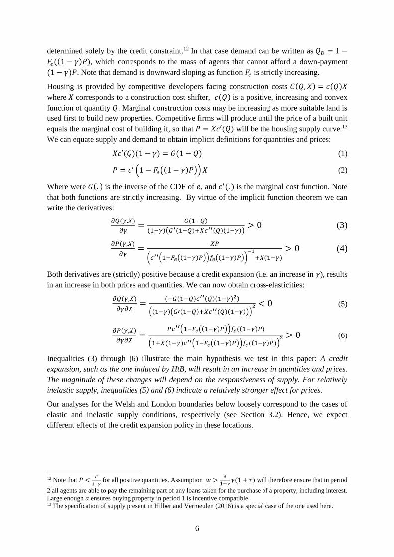
2.2. Theoretical Framework

In this sub-section we develop a simple theoretical framework—a partial equilibrium model of

the housing market with heterogeneous households, featuring credit constraints and endogenous

housing supply—to guide our empirical analysis.9 The model illustrates how a relaxation of

credit conditions affects housing quantity and prices, depending on the costs of developing new

stock.

The framework is partial equilibrium in that it abstracts from the possibility that a relaxation of

credit conditions in one location could affect supply or demand in other locations. Yet both

prices and quantities are endogenous. A relaxation of credit conditions will lead to both an

increase in the price and an expansion in quantity. The relative magnitude of the two effects

depends on the price elasticity of supply. For low (high) supply elasticities, the price effect is

stronger (weaker) and the quantity effect weaker (stronger). Differences in the elasticity of

supply arise from varying costs of developing land in different locations. The theoretical

insights from this framework can be summarized by the cross-elasticities of quantity and prices

taken over the credit condition parameter and the cost of a building shifter.10

Suppose a two-period economy with a unit mass of households which can buy property in a

given location in period 1. These households have preferences over consumption c and

ownership-location amenity 𝑎 , as given by a period utility 𝑢(𝑐, 𝑎) which is continuous,

increasing and differentiable in both arguments, with limits satisfying standard assumptions.11

Households can only obtain 𝑎 > 0 if they buy a housing unit in the location and obtain 0

otherwise. This is consistent with both, a model in which renting is not possible and a model,

where 𝑎 captures the warm-glow from ownership (Iacoviello and Pavan 2013, Kiyotaki et al.

2011, Carozzi forthcoming). The discount factor is β.

Households receive an endowment 𝑒 in period 1 and a location specific income 𝑤 in period 2

which can be used for consumption or to buy property. Households are heterogeneous in the

initial endowment 𝑒, which is continuously distributed over the positive interval [𝑒, 𝑒] with

cumulative density function 𝐹𝑒 . Housing units in the location are homogeneous and can be

bought in period 1 for endogenous price P. Credit is available for the purchase of the property,

yet a minimum down-payment, corresponding to a fraction (1 − 𝛾) of the property value is

required. Credit and savings pay interest 𝑟 . We assume 𝑤 > �̅�𝛾(1 + 𝑟)/(1 + 𝛾) . This

assumption ensures that, for sufficiently large 𝑎 , demand for housing in the location is

9 The model builds on Hilber and Vermeulen (2016) who consider a similar setting but abstract from the role of

credit conditions. 10 The model presented here introduces credit conditions via a change in required loan-to-value ratios (LTVs), as

is customary in the literature. We treat housing as homogeneous, with all units being identical. An extension with

two types of units in which credit conditions only change for units at the lower end of the market yields very

similar insights. 11 Specifically, lim

𝑎→∞𝑢(𝑐, 𝑎) = ∞ if 𝑐 > 0 , lim

𝑐→∞𝑢(𝑐, 𝑎) = ∞ if 𝑎 > 0 , and 𝑢(𝑐, 𝑎) > 0 ∀𝑐, 𝑎 ≥ 0 .Note these

assumptions are satisfied for both the linear additive and Cobb-Douglas specifications.

6

determined solely by the credit constraint.12 In that case demand can be written as 𝑄𝐷 = 1 −

𝐹𝑒((1 − 𝛾)𝑃), which corresponds to the mass of agents that cannot afford a down-payment

(1 − 𝛾)𝑃. Note that demand is downward sloping as function 𝐹𝑒 is strictly increasing.

Housing is provided by competitive developers facing construction costs 𝐶(𝑄, 𝑋) = 𝑐(𝑄)𝑋

where 𝑋 corresponds to a construction cost shifter, 𝑐(𝑄) is a positive, increasing and convex

function of quantity 𝑄. Marginal construction costs may be increasing as more suitable land is

used first to build new properties. Competitive firms will produce until the price of a built unit

equals the marginal cost of building it, so that 𝑃 = 𝑋𝑐′(𝑄) will be the housing supply curve.13

We can equate supply and demand to obtain implicit definitions for quantities and prices:

𝑋𝑐′(𝑄)(1 − 𝛾) = 𝐺(1 − 𝑄) (1)

𝑃 = 𝑐′ (1 − 𝐹𝑒((1 − 𝛾)𝑃)) 𝑋 (2)

Where were 𝐺(. ) is the inverse of the CDF of 𝑒, and 𝑐′(. ) is the marginal cost function. Note

that both functions are strictly increasing. By virtue of the implicit function theorem we can

write the derivatives:

𝜕𝑄(𝛾,𝑋)

𝜕𝛾=

𝐺(1−𝑄)

(1−𝛾)(𝐺′(1−𝑄)+𝑋𝑐′′(𝑄)(1−𝛾))> 0 (3)

𝜕𝑃(𝛾,𝑋)

𝜕𝛾=

𝑋𝑃

(𝑐′′(1−𝐹𝑒((1−𝛾)𝑃))𝑓𝑒((1−𝛾)𝑃))−1

+𝑋(1−𝛾)

> 0 (4)

Both derivatives are (strictly) positive because a credit expansion (i.e. an increase in 𝛾), results

in an increase in both prices and quantities. We can now obtain cross-elasticities:

𝜕𝑄(𝛾,𝑋)

𝜕𝛾𝜕𝑋=

(−𝐺(1−𝑄)𝑐′′(𝑄)(1−𝛾)2)

((1−𝛾)(𝐺′(1−𝑄)+𝑋𝑐′′(𝑄)(1−𝛾)))2 < 0 (5)

𝜕𝑃(𝛾,𝑋)

𝜕𝛾𝜕𝑋=

𝑃𝑐′′(1−𝐹𝑒((1−𝛾)𝑃))𝑓𝑒((1−𝛾)𝑃)

(1+𝑋(1−𝛾)𝑐′′(1−𝐹𝑒((1−𝛾)𝑃))𝑓𝑒((1−𝛾)𝑃))2 > 0 (6)

Inequalities (3) through (6) illustrate the main hypothesis we test in this paper: A credit

expansion, such as the one induced by HtB, will result in an increase in quantities and prices.

The magnitude of these changes will depend on the responsiveness of supply. For relatively

inelastic supply, inequalities (5) and (6) indicate a relatively stronger effect for prices.

Our analyses for the Welsh and London boundaries below loosely correspond to the cases of

elastic and inelastic supply conditions, respectively (see Section 3.2). Hence, we expect

different effects of the credit expansion policy in these locations.

12 Note that 𝑃 <

�̅�

1−𝛾 for all positive quantities. Assumption 𝑤 >

�̅�

1−𝛾𝛾(1 + 𝑟) will therefore ensure that in period

2 all agents are able to pay the remaining part of any loans taken for the purchase of a property, including interest.

Large enough 𝑎 ensures buying property in period 1 is incentive compatible. 13 The specification of supply present in Hilber and Vermeulen (2016) is a special case of the one used here.

7

3. Empirical Analysis

3.1. Data and Descriptive Statistics

Our empirical analysis employs geo-located data on housing sales in England and Wales,

including information on unit characteristics and transaction prices. Our main data source is the

Land Registry Price Paid Dataset, which covers the vast majority of residential transactions in

England and Wales. This source includes property transactions from 1995 to 2018, recording

the transaction price, postcode, address, the date the sale was registered (which proxies for the

transaction date), and categorical data on dwelling type (detached, semi-detached, flat or

terrace), tenure (freehold or leasehold) and whether the home is a new build property.

Our main estimation sample uses transaction data from 2012 to 2018, which includes a total of

6,366,690 transactions, of which 11% are transactions of new build units. All transactions are

geo-coded using address postcodes. We then select all the new build transactions near the GLA

boundary and the English/Welsh border for our spatial discontinuity designs. We replicate our

analysis using new build transactions near the Greater Manchester boundary as a placebo test.

We also utilize Energy Performance Certificate (EPC) data that contains information on the

floor area and other physical characteristics of newly built units. We match this data to the Land

Registry (LR) in order to augment the latter dataset with additional information on the

transacted newly built units.14

Demographic and neighborhood characteristics at LSOA level are collected from the 2011

Census. These variables (interacted with year dummies) are used as controls and are the

percentage of (1) married residents and (2) residents with level-4 and above educational

qualifications. We use the National Statistics Postcode Lookup Directory to match postcodes

to coordinates and LSOAs. To construct the baseline estimation sample for the price effect, we

select all the new build transactions within 5 kilometers from the GLA boundary and Greater

Manchester boundary, and within 10 kilometers from the English/Welsh border.15 We then

merge these selected Land Registry transactions with the EPC dataset and Census data to

control for a wide range of neighborhood and hedonic housing characteristics.

Basic summary statistics computed for a sample of housing transactions within 5 kilometers of

the GLA boundary from January 2012 to December 2018 are detailed in Panel A of Table 2.

There are 32,127 newly built property transactions in this area. The average value of the house

price is £394,703, and the average size of these properties is 87.2 square meters. Panel B of

14 EPCs provide information on buildings consumers plan to purchase or rent. Since 2007 an EPC has been required

whenever a home is constructed or marketed for social rent, private rent or sale. We use a dataset that contains all

EPCs issued between 2008 and 2019. The dataset includes the type of transaction that triggered the EPC, the

energy performance of properties and their physical characteristics. Following Koster and Pinchbeck (2017), we

merge the EPC data into the Land Registry (LR) dataset using a sequential match strategy. First, we match a LR

sale to certificates using the primary address object name (PAON; typically, the house number or name), secondary

address object name (SAON; typically, the identification of separate unit/flat), street name, and full postcode. We

then retain the certificate that is closest in days to the sale or take the median value of characteristics where there

is more than one EPC in the same year as the sale. We then repeat this exercise for unmatched properties but allow

one of the PAON or SAON to be different. Our final round of matching is on the full postcode. The matched

dataset provides us total floor area; whether the property has a fireplace or not; total energy consumption and total

CO2 emission of the property. 15 The number of transactions for the resulting samples are reported in Appendix Table B1. This table also reports

sample sizes for smaller bands around the respective boundaries.

8

Table 2 shows the descriptive statistics for a baseline sample of new build transactions within

10 kilometers of the English/Welsh border from 2012 to 2018. The average value of house price

there is £234,202, and the average size of these properties is 102.2 square meters.

When estimating the effect of the policy on housing construction, we assemble a ward by month

panel using data from January 2012 to December 2018. We obtain ward-level observations by

aggregating from individual new build sales. Panels C and D of Table 2 document the

descriptive statistics of our estimation sample for the construction effect. The datasets for the

GLA boundary-area and the English/Welsh border-area consist of 436 wards and 272 wards

respectively. The propensity for having at least one new build transaction in any month is 0.2

for the GLA sample and 0.13 for the English/Welsh sample. On average, 0.88 new builds are

transacted each month near the GLA boundary and 0.37 near the English/Welsh border.

We construct an additional dataset in the form of a developer/construction company panel,

covering 84 companies over the same period as the transaction level dataset (2012-2018). We

label the full sample of 84 developers our difference-in-differences sample. The panel includes

financial information of these companies from Orbis. It also includes information on whether

these companies are registered with a HtB agency or not. A builder must be registered with one

of the regional government offices managing the scheme for its properties to be eligible for an

equity loan. Finally, we include hand-coded data on the fraction of properties sold through the

scheme from annual reports in a selected sample of 30 residential developers. This is our

intensity sample. The large sample of 84 companies is obtained after combining a list of the

main builders in the United Kingdom from Zoopla – one of the main property websites in the

country – and financial data from Orbis. This list includes residential developers, commercial

developers and construction companies.

3.2. The Role of Local Supply Conditions

We compare estimates of the effect of HtB obtained from a sample of properties near the GLA

boundary with a sample of properties from near the English/Welsh border as well as with a

sample derived from properties near the Greater Manchester boundary. We choose the first two

areas because they both provide an ideal quasi-natural setting to identify the economic effects

of HtB. We use the area near the Greater Manchester boundary for our placebo tests, as the

same HtB policies and thresholds apply inside and outside of that boundary.

One crucial difference between our two focal areas – the area near the GLA boundary and the

area near the English/Welsh border – is that the former has overall vastly more unresponsive

supply, driven by both, tighter local planning regulations as well as a greater relative scarcity

of undeveloped developable land. Theory thus suggests that the positive impact of HtB on house

prices should be much larger and the positive impact on new construction much smaller in the

area near the GLA boundary.

In order to illustrate the differences in supply conditions between the areas, we employ a

number of measures that capture long-term housing supply constraints. These measures are the

share of land designated as green belt (provided by the Ministry of Housing, Communities and

Local Government), the average planning application refusal rate taken over the period from

1979 to 2008, the average share of developed developable land, and the average elevation range

9

(all derived from Hilber and Vermeulen, 2016). We calculate these measures for all three areas16

using Local Planning Authority (LPA)-level data and LPA surface areas as weights.

Table 3 (rows 1 to 4) illustrates the differences in supply conditions between the three areas.

The most striking difference between the two focal areas lies in the share of ‘green belt’ land.

Land in green belts is typically off limits for any development (residential or commercial) and

thus represents a ‘horizontal’ supply constraint. This share is 66.5% for boroughs along the

boundary of the GLA but only 3.8% for English boroughs along the English/Welsh border.

Another measure to capture physical supply constraints is the share of developable land already

developed. This share is 27.6% for boroughs along the GLA boundary but only 6.3% for

English boroughs along the English/Welsh border.

The arguably quantitatively most important long-term supply constraint are restrictions

imposed by the British planning system (Hilber and Vermeulen 2016). The weighted average

of this refusal rate is 35.6% for boroughs along the GLA boundary and 27.2% for English

boroughs along the English/Welsh border.

While the area near the English/Welsh border is subject to greater topographical (slope related)

supply constraints, Hilber and Vermeulen (2016) demonstrate that these constraints, while

statistically significant, are quantitatively unimportant in explaining local price-earnings

elasticities.

Lastly, it is important to point out that the area near the GLA boundary is not only characterized

by vastly more restrictive supply conditions, but these constraints are also significantly more

binding in practice, simply because aggregate housing demand there is much stronger. To

illustrate this point, consider a ten-story height restriction in the heart of a superstar city such

as London and compare it to the same constraint in the desert. The restriction is extremely

binding in the former location, while completely irrelevant in the latter.

To explore the differences in supply responsiveness across the three areas further, we employ

the estimated coefficients from Hilber and Vermeulen (2016) to compute an implied house

price-earnings elasticity. Table 3 (rows 5 and 6) reports our estimated elasticities based on these

coefficients. Using the OLS estimates, we find, consistent with our priors, that the price-

earnings elasticity along the GLA boundary (0.40) is higher than that of the area along the

Greater Manchester boundary (0.28), which in turn is higher than the elasticity of the area near

the English/Welsh border (0.25). As two of the three supply constraints measures employed in

their estimation, refusal rate and share developed land, are likely endogenous, we employ the

instrumental variable strategy proposed in Hilber and Vermeulen (2016). This provides

exogenous variation in our supply constraint measures, which we use to re-compute the

unbiased price-earnings elasticities. The rank order remains unchanged. The GLA has again the

highest elasticity (0.21) followed by Greater Manchester (0.16) and the English/Welsh border

area (0.13).

The higher price-earnings elasticity along GLA boundary suggests that due to local supply

constraints, housing prices respond more strongly to a given change in local housing demand.

16 We do not currently have data for LPAs on the Welsh side of the English/Welsh border. We will incorporate

these figures in a subsequent paper version. We expect that the differences between the GLA and the

English/Welsh border will be even more striking when taking account of the Welsh LPAs.

10

This also implies a lower supply price elasticity in the GLA boundary area. In the next section,

we outline our identification strategy and discuss how we measure the impact of HtB on house

prices and construction activity.

3.3. Identification Strategy and Empirical Specifications

Our empirical strategy is designed to test the impact of HtB on housing construction and house

prices. We exploit spatial differences in the intensity of the HtB policy. As mentioned above,

HtB Wales was rolled out nine months later than in England, and offered a government-backed

loan for the purchase of new build properties under £300,000 (£600,000 in England). There

were also differences in the intensity of the HtB policy between the GLA and its surroundings,

starting in 2016. In this case, the difference lies in the size of the government-backed loan

available to households. London-HtB offered loans of up to 40% of a new build’s value, while

this figure was 20% elsewhere (i.e., outside the GLA boundary). We exploit these regional

differences in policy in a differences-in-discontinuities design combining time variation in

prices and new build construction with local variation in policy intensity around the regional

boundaries.

The samples of new build properties used in the analyses of prices and construction effects near

the English/Welsh border and the GLA boundary are illustrated in Figures 1 and 2,

respectively.17 Our boundary approach is meant to ensure that we are comparing properties

affected by similar economic and amenity shocks, as compared to a standard Difference-in-

Differences strategy that simply takes whole regions as control groups. The identifying

assumption in both cases can be likened to the typical assumption of parallel trends: in the

absence of the policy, prices and construction on either side of the boundary would have

followed a parallel evolution over time. Figure 3 and Figure 4 depict the house price index at

the GLA boundary and English/Welsh border respectively prior to and post HtB, indicating that

prices move in parallel prior to the implementation of the policy.

We complement these strategies by studying bunching in new build property prices around the

£600,000 price threshold in England to show whether HtB affected the type of properties

offered by developers. This specific analysis further elucidates developers’ responses to the

policy beyond those provided in our boundary analysis.

3.3.1. Specification: Impact of Help to Buy on House Prices

The HtB policy is meant to operate as a relaxation of households’ credit constraints. Hence, it

can lead to an increase in demand for new builds, and as a result, to an increase in the price of

new builds. To test this, we use observed transactions of new build units close to the boundary

of the GLA and the English/Welsh border. We conduct both exercises separately. We first

provide graphs of prices at different distances to the boundaries before and after the differences

in HtB intensity arise, including flexible polynomials in distance to illustrate how the

differences in prices at the boundary change with the policy. To estimate the magnitude of these

differences in our differences-in-discontinuities framework we estimate:

ln(𝑃𝑖𝑡) = 𝜙𝑝 + 𝛽𝐻𝑇𝐵𝑖𝑡 + 𝛿𝑡 + 𝛾′𝑋𝑖𝑡 + 𝑓(𝐷𝑖𝑠𝑡𝑎𝑛𝑐𝑒𝑖) + 𝛾𝑦𝐷𝑖𝑠𝑡𝑎𝑛𝑐𝑒𝑖 × 𝑑𝑦 + 휀𝑖𝑡 (7)

17 Appendix Figure A1 depicts the corresponding map for our placebo sample, properties near the Greater

Manchester boundary.

11

where 𝑖 indexes individual properties and 𝑡 indexes time periods. The variable 𝐻𝑇𝐵𝑖𝑡 is a

dummy that takes value 1 in the region with a more generous HtB policy (i.e. inside the GLA

or on the English side of the Welsh/English border) after the difference in policy takes place. A

vector of postcode fixed effects is represented by 𝜙𝑝, 𝛿𝑡 is a set of time dummies and 𝑋𝑖𝑡 is a

set of controls including housing characteristics as well as neighborhood characteristics (from

the 2011 Census) interacted with year dummies. In every specification we control for distance

to the boundary by estimating different linear terms on either side. After we control for postcode

fixed effects, we include distance to boundary interacted with year dummies to account for

potential time varying shocks that differ spatially. We estimate this equation by OLS, clustering

standard errors at the postcode-level to account for potential spatial correlation in local price

shocks. This is estimated on properties at specific bandwidths around the corresponding

boundaries. In the case of the London HtB, we use a 5km bandwidth around the GLA boundary.

Because transactions near the English/Welsh border are sparser, we use a 10km bandwidth for

that exercise. In the robustness checks section, we show that our results are robust to these

specific bandwidth choices.

Our parameter of interest is 𝛽. It measures the effect of differences in the intensity of the HtB

policy on the price of new build properties.

3.3.2. Specification: Impact of Help to Buy on Housing Construction

The government’s equity loan is available only for the purchase of new build units. In this way,

the government attempts to ensure the policy results in a supply response by developers. In

order to test whether this is the case, we estimate the effect of differences in the intensity of the

policy on both sides of the regional boundaries mentioned above on construction activity.

Again, we use a difference in discontinuities specification. This exercise is conducted by

aggregating new build counts at the ward level for every month. As in the exercise for prices,

we first provide graphs of the differences in new building activity at different distances from

the boundary. Next, we estimate:

𝑁𝑒𝑤 𝑏𝑢𝑖𝑙𝑑𝑠𝑗𝑡 = 𝜔𝑗 + 𝛽𝐻𝑡𝐵𝑗𝑡 + 𝛿𝑡 + 𝑓(𝐷𝑖𝑠𝑡𝑎𝑛𝑐𝑒𝑗) + 𝛾𝑦𝐷𝑖𝑠𝑡𝑎𝑛𝑐𝑒𝑗 × 𝑑𝑦 + 휀𝑗𝑡 (8)

Where 𝑗 indexes wards and 𝑡 indexes periods. The dependent variable is now 𝑛𝑒𝑤 𝑏𝑢𝑖𝑙𝑑𝑠𝑗𝑡,

which can represent either the number of new build transactions in ward 𝑗 and period 𝑡, or a

dummy taking value 1 if there are any new build sales in ward 𝑗 and period 𝑡. The variable

𝐻𝑡𝐵𝑖𝑡 is a dummy taking value 1 in the region with a more generous HtB policy (i.e., inside the

GLA boundary or on the English side of the English/Welsh border) after the difference in policy

arises. We include a set of ward fixed effects, represented by 𝜔𝑗 and time fixed effects 𝛿𝑡. We

also control flexibly for distance between the ward centroid and the boundary by including two

linear terms in distance, estimated separately on each side. After we control for ward fixed

effects, we include distance to boundary interacted with year dummies to account for potential

time varying shocks that differ spatially. In all specifications we cluster standard errors at the

ward level to account for potential spatial correlation. We estimate our specification using

observations within 5km of the boundary in the case of the London GLA, and 10km in the case

of the English/Welsh border.

12

Our parameter of interest is 𝛽, measuring the effect of differences in the intensity of HtB on

new construction. Because the differences in intensity are not the same across the

English/Welsh border and across the GLA boundary, we will obtain separate estimate for these

two exercises.

3.3.3 Help-to-buy and Developers’ Financial Performance

By inducing an increase in demand for new build housing, help to buy may have an impact

on the financial performance of firms participating in the design, planning and building of

residential units. On the first place, the policy should induce an increase in revenue of existing

developers.18 Moreover, barriers to entry and imperfect competition in the housing production

and land markets imply the policy could also translate into increases in profits. This last point,

however, depends on whether the increase in revenues is neutralized by an increase in the costs

of land after the policy is implemented. Uncovering how HtB affected the performance of

developers can therefore identify some of the beneficiaries of this policy.

To study this empirically, we use our developer dataset which financial information for 84 large

British developers and construction companies. Crucially, our dataset includes information on

the participation of these firms in HtB. We use this dataset to compare how the change in

performance of firms before and after 2013 varied with their participation in HtB. For this

purpose, we estimate a fixed effect model specified as:

𝐹𝑖𝑛𝑎𝑛𝑐𝑖𝑎𝑙𝑖𝑡 = 𝛽𝐻𝑡𝐵𝑖 × 𝑃𝑜𝑠𝑡𝑡 + 𝛼𝑖 + 𝛿𝑡 + 휀𝑖𝑡 (9)

𝐹𝑖𝑛𝑎𝑛𝑐𝑖𝑎𝑙𝑖𝑡 is an indicator of financial performance for developer 𝑖 in year 𝑡. We look at

turnover (i.e. total revenues), gross profits, net profits before taxes and the difference between

gross and net profits. 𝐻𝑡𝐵𝑖 is a measure of the developer’s participation in the program. We use

two different definitions of this variable depending on the information available and therefore

conduct the analysis on two separate samples. Our intensity sample consists of the 30

developers for which we know the fraction of the units produced that were sold under the HtB

scheme. We average this figure over time to obtain a time-invariant average fraction of units

by developer. Our second definition of 𝐻𝑡𝐵𝑖 is based on the registry of developers in regional

HtB offices across the country. In this case, the variable is a dummy taking value 1 if the

developer is included in the registry. The information on registrations is available across a larger

group of firms, so we can estimate this specification for our larger differences-in-differences

sample of 84 developers. Variable 𝑃𝑜𝑠𝑡𝑡 is a variable taking value 1 after 2012. Finally, 𝛼𝑖 is a

developer fixed-effect and 𝛿𝑡 represents a set of year dummies.

Estimates of 𝛽 will measure the impact of the policy of firms and revenues under the

assumption that unobservables 휀𝑖𝑡 are uncorrelated with 𝐻𝑡𝐵𝑖 × 𝑃𝑜𝑠𝑡𝑡 conditional on

individual and year effects. Because firms actively self-select into the program, the identifying

assumption requires that the difference in performance between firms that self-select into the

scheme and does that do not is fixed over time. In other words, other shocks to performance in

the 2010-2018 period are uncorrelated with program participation.

18 The increased supply could in principle by taken up exclusively by new entrants. Yet the presence of economies

of scale in housing production and the learning curve required to navigate the British planning system mean the

volume of new entrants will probably be very small.

13

3.3.4. Bunching Analysis

The English HtB policy is only available for properties purchased under 600,000 GBP. We can

use this threshold to study bunching of property sales close to this price level. In doing so, we

apply some of the methods recently developed in Chetty et al. (2011), Kleven (2016) and Best

and Kleven (2017). The purpose of this analysis is two-fold. First, we want to test whether HtB

induced a change in the type of properties supplied by developers. In addition, we want to obtain

an alternative method to study the effect of the policy on building volumes. We first document

that indeed there is substantial bunching at the £600,000 price threshold. Next, we construct a

counterfactual distribution of new builds at different price levels using information on sales

excluding the region around the bunching thresholds. Following Kleven (2016), we estimate

this counterfactual distribution by calculating the number of new build transactions in 5000

GBP bins and using these to estimate:

𝑆𝑙𝑡 = ∑ 𝑝𝑙𝑡𝑞3

𝑞=0 + ∑ 𝜌𝑟1 {𝑝𝑗

𝑟∈ ℕ} + 휀𝑙𝑡𝑟∈𝑅 (10)

where 𝑙 indexes price bins and 𝑡 indexes time. The dependent variable 𝑆𝑙𝑡 measures the number

of new build transaction in bin 𝑙 at time 𝑡. The first two sums correspond to the estimate of the

counterfactual price distribution. The first sum is a third degree polynomial on the distance

between price bin l and the cutoff of £600,000, and q is the order of the polynomial. The second

sum estimates fixed effects for round numbers with ℕ representing the set of natural numbers

and 𝑅 = {5000, 10000, 25000, 50000} representing a set of round numbers. We estimate this

equation with data for new build transactions in England taking place after April of 2013 (the

introduction of HtB in England). We then obtain differences between this estimated

counterfactual distribution and the observed distribution of prices to estimate bunching effects

induced by HtB.

The difference between the size of the spike just under the threshold and the gap just after the

threshold can be used to estimate the size of the local effect of HtB on new building activity.

This can be driven by changes in the types of properties sold after accounting for local shifting

in prices induced by the policy.

3.4. Main Results

3.4. 1. Visual Evidence of Boundary Discontinuity

We first provide a series of graphs illustrating the main results in our paper. Figure 5 represents

the prices for newly built units at different distances from the GLA boundary. Positive distances

correspond to locations inside the GLA, and negative distances to locations outside of this area.

Circles depict the mean value of new build house prices for 500-meter-wide distance bins with

the size of each circle being proportional to the number of observations in that bin. Lines in

both panels represent fitted values from 2nd order polynomials estimated separately on each side

of the boundary. Gray bands around them represent 95% confidence intervals.19 Panels A and

B illustrate results before and after the introduction of London HtB, respectively. Comparing

both panels, we find that a discontinuity in prices at the boundary emerges after the

19 We report 2nd degree polynomials in these figures because they yield a lower Akaike Information Criterion

statistic than 1st degree polynomials. Appendix Figure A2 reports results when using linear equations on either

side of the threshold.

14

implementation of London’s HtB. We interpret this as evidence that this scheme has a

significant and positive effect on the price of newly built properties.

Figure 6 illustrates our results for the new build price effect at the English/Welsh border. Circles

depict the mean value of house prices for 1000-meter-wide distance bins. As above, solid lines

represent 2nd degree polynomials estimated on both sides of the boundary.20 In this case,

however, we do not observe a spatial discontinuity of house prices in either Panel A or B.

We conduct a similar exercise looking at changes in construction volumes at these boundaries

before and after the corresponding changes in HtB. Results are illustrated in Figures 7 and 8.

The former shows construction as measured by new build sales near the GLA boundary with

Panels A and B corresponding to the periods prior and post implementation of London HtB,

respectively. We do not find a spatial discontinuity in homebuilding at the London boundary in

either period. Figure 8 shows results for English/Welsh border before and after the English HtB

policy was rolled. In this case, we find a clear discontinuity emerging in Panel B, indicating

more building took place on the English side of the boundary after the policy was introduced.

Finally, we conduct a placebo experiment using properties sold around the greater Manchester

boundary to test whether any spatial discontinuities in prices emerge after the introduction of

London HtB in 2016. Note that the intensity of the policy is identical inside and outside the

Manchester boundary. Results are provided in Figure A4 in the Appendix. As expected, we

observe no discontinuity in prices at the boundary before or after the London HtB policy was

put in place.

Overall, these graphs indicate that more generous versions of the policy triggered a price

response in the supply inelastic areas around London. Conversely, the policy generated a

quantity response in the relatively supply elastic areas around the English/Welsh border. This

is in line with the intuition that price or quantity responses to shifts in demand depend on the

shape of the supply curve, as illustrated in the theoretical framework provided in Section 2.2.

In the following two sections, we present reduced-form estimates for the magnitudes of these

effects.

3.4.2. Effect of HtB on House Prices

Table 4 summarizes the results from estimating equation (7) using the sample of transactions

of new build properties within 5 kilometers from the GLA boundary. Additional covariates are

included into the estimation sequentially from columns 1 to 5. Column 1 controls for time

effects and independent linear terms in distance of each property to the GLA boundary. Column

2, adds a vector of housing characteristics such as total floor area, type of the property, tenure

of the property. Column 3 adds postcode fixed effects. In column 4, we allow for heterogeneous

spatial price trends by controlling for interactions between distance from the GLA boundary

and year dummies. Finally, column 5 includes a set of neighborhood controls. Our preferred

specifications are those including property characteristics, as it is likely that the policy would

affect the characteristics of sold units.21 The standard errors in all specifications are clustered

at the postcode level to allow for a degree of spatial correlation in the error term.

20 Appendix Figure A3 reports results when using a linear polynomial. 21 We return to this point in Section 3.5.2.

15

The resulting estimates show that London’s HtB policy increased newly built house prices

inside the GLA by between 4.5% and 6.5% depending on the specification. All estimates are

significant at the 5% level. The average property price in this sample is £394,703, so this finding

suggests that homebuyers are paying £23,682 more to buy newly built properties inside the

GLA because of London HtB. In Section 3.7, we compare this effect to that which would result

from the implicit interest subsidy provided by the equity loan granted by the scheme.

Table 6 summarizes the results from estimating equation (7) for the sample of properties around

the English/Welsh border. Again, we successively include additional controls from columns 1

to 5. Once we control for postcode fixed effects, we observe no significant effect of the policy

on the price of new build sales. The point estimates in columns 3 to 5 are positive but small,

ranging between 1.7 and 2.4%, and not statistically significant, with p-values above 0.4 in all

of these specifications.

These estimates confirm the results reported in the graphical analysis provided in Section 3.4.2

and are also in line with the predictions highlighted in our theoretical framework. As land

supply is relatively inelastic near the GLA boundary, the shift in demand induced by HtB is

capitalized into prices. Near the English/Welsh border, where developable land is available, the

response is more likely to happen in quantities. Naturally, this hypothesis is testable; we

estimate the effect of HtB on housing supply in the next section.

3.4.3. Effect of HtB on Housing Construction

Table 6 summarizes the results from estimating equation (8) for the sample including all wards

within 5 kilometers of the GLA boundary. We define the post-HtB period as extending from

Q1 2017 to Q4 2018, – starting one year after the implementation of London’s HtB – to allow

for a one-year construction lag. From Table 6, we observe that London HtB did not have a

significant effect either on construction volumes or on the probability that any newly built

property was sold in a ward. Coefficients are insignificant and small in all specifications,

indicating that the policy did not lead to an increase in housing supply.

In Table 7, we provide estimates of equation (8) for wards around the English/Welsh border.

As above, the post-treatment period is defined as starting one year after the introduction of the

English HtB. We find a significant and positive effect of HtB on housing construction in all

specifications. Our estimate suggests that HtB increases the number of new build transactions

at each ward by 0.355 on average, and the propensity for any new build construction at each

ward by 6.67%. These results are consistent with the predictions from our theoretical

framework indicating HtB will have differential effects in London and the areas around Wales

as a consequence of differences in supply elasticities between both areas.

3.4.4. Effect of HtB on Financial Performance of Developers

Our findings in previous sections indicate that HtB increased demand, translating into higher

housing prices or building output. How did this affect the financial performance of residential

developers? Table 8 presents our estimates for the effect of the scheme on revenues, gross

profits and net profits before taxes, obtained from a developer panel as detailed in Section 3.4.4.

Panel A presents estimates of the effects for our continuous measure of HtB participation. The

first column shows a 1 percentage-point increase in the fraction of HtB properties supplied by

that developer leads to a 1.1% increase in revenues. The effect is large and significant. The

16

estimates for gross profits and net profits, displayed in columns 2 and 3 are even larger,

indicating that changes in costs – e.g. costs of acquiring land – did not neutralize the changes

in revenue. Hence, these estimates suggest that the policy improved the performance of

residential developers. The estimate in column 4 measures the effect of the policy on operating

and interest expenses, obtained by taking the difference between gross and net profits. The

effect is positive and significant for both samples.

Panel B of Table 8 shows estimates using our larger differences-in-differences sample, where

participation in HtB is measured using a dummy variable taking value 1 if the developer is

registered with one of the regional HtB offices in the country. Participation in the program

appears to increase revenues substantially, with program participants obtaining over 70%

higher revenues than non-participants.22 Again, the coefficients for gross and net profits are

even larger. The estimate in column 4 of Panel B tells us that operating plus interest expenses

of companies registered with the program increased by 34% relative to the control group. The

policy is unlikely to have had an impact of financing costs, so we interpret this as suggestive

evidence that the scheme affected the operating costs of the developers, possibly including

management costs.

In Figure 9, we display yearly average profits adjusted for individual company fixed-effects for

the HtB and non-HtB groups of developers before and after the policy. The pre-trends are

reasonably parallel, and we observe a divergence after 2013, with substantial growth for

developers registered for HtB. These results reinforce the notion that developers improved their

financial performance as a result of Help-to-buy. An additional implication is that, on the supply

side of the residential market, the benefits of the scheme did not go exclusively to land owners.

Some caution is warranted when interpreting these findings. Both the intensity and difference-

in-difference samples used to produce the estimates in Table 8 cover a small number of

relatively large developers and are only partially representative of the population. In addition,

there are substantial observable differences in characteristics between the developers self-

selecting into the scheme and other developers in the sample. For example, luxury developers

typically fall in the control group, as they will not normally be registered with HtB. Our

estimates can be interpreted causally only if we consider that these differences have a time-

invariant influence on performance. Unfortunately, lack of detailed information on the location

of developers’ assets prevents us from deploying the spatial techniques used in our analysis of

price and construction effects.

3.5. Additional Results

3.5.1. Bunching Effect

We now turn to documenting that the English HtB program led to significant bunching of sales

right below the price threshold. Figure 10 shows two histograms of new build frequencies for

prices between £550,000 and £650,000. The left-panel represents properties sold in the period

from Q1 2010 to Q1 2013, before the implementation of HtB in England. The right-panel

corresponds to histogram for properties sold between Q2 2013 and Q4 2018, after HtB was

22 The coefficient 𝛽 is 0.5374, so we can write the proportional difference in revenues is Δ𝑟 = 𝑒0.5347 − 1.

17

introduced. We can observe a substantial increase in the amount of bunching in the price

distribution of new builds just below £600,000 taking place between both periods.

We provide two alternative ways of showing the bunching at this price point in figures A5 and

A6 of the Appendix. To produce Figure A5, we first group sales into £10,000 price bins and

then plot the evolution of the fraction of new builds over total sales for each bin from 2010 to

2018. The black line represents the price bin of interest, £590,000 to £600,000. Grey lines

correspond to the other bins between £510,000 and £700,000. The gaps between the black line

and the grey lines increase substantially from 2015, implying a significant amount of bunching

of new builds at £600,000 after this year. Figure A6 shows the fraction of new builds over total

sales for £5000 price bins. Horizontal dashed lines represent averages above and below the

£600,000 threshold. We also observe significant bunching at £600,000.

Finally, Figure A7 illustrates the difference between the observed density of property

transactions and our estimated counterfactual density around the £600k notch.23 We observe

substantial bunching below the cut-off of £600,000 and a large hole in the distribution above

the cut-off. Using our counterfactual price distribution, we estimate there are 2,033 more

transactions for properties valued from £590,000 to £600,000 and 982 less transactions for

properties valued from £600,000 to £630,000.24 These estimates suggest that HtB leads to a

significant shift in housing construction away from properties above the price threshold,

towards properties below the threshold.

3.5.2. Size Effect

Figure A8 provides a descriptive analysis of the impact of HtB on the size of newly constructed

units at the English/Welsh border. Circles depict the mean value of new build housing size for

2000-meter-wide distance bins. The size of each circle is proportional to the number of

observations in that bin. Panel A represents the housing size before the English version of HtB

was put in place, while Panel B depicts the housing size after the scheme was rolled out. Lines

in both panels represent 2nd order polynomial fits of housing size on the distance to the

English/Welsh border, with the band around them representing 95% confidence intervals.

Comparing Panels A and B, we find a sharp discontinuity in the total floor area of new build

properties at the boundary after the implementation of the English HtB. This result provides

strong evidence that HtB has a significant and negative association with the size of newly built

properties.

Next, we apply a difference-in-discontinuities design to estimate the effect of HtB on the size

of newly built housing units. Table B2 summarizes the results. We estimate the new build

transactions between £300,000 and £600,000 within 20 kilometers from the English/Welsh

border. We assume that the post-HtB period starts from April 2014, one year after the

implementation of the English HtB. We include additional variables sequentially from columns

1 to 5. Only the coefficients and standard errors for the key treatment estimates of HtB are

reported. We observe that HtB has a significant and negative effect on the total floor area of

properties. The estimated results are robust across all specifications.

23 See Section 3.3.3 for details on the estimation of this counterfactual density. 24 These numbers amount, respectively, to 10.4% and 5% of all sales in the £550000-£650000 range.

18

Our estimation results suggest that HtB decreases the size of newly built housing units on the

English side of the English/Welsh border by 6.73%. Although HtB does not have a significant

price effect at the border, it does decrease the size of newly constructed units. Tables B3 and

B4 report the results of two corresponding placebo tests (replicate estimation for new build

transactions valued less £300,000 and for new build transactions between 2010 and 2014). We

do not find significant effects.

3.5.3. Credit Supply Effect

We use mortgage lending data from UK Finance to measure the effects of HtB on mortgage

origination inside the GLA boundary. UK Finance data covers mortgage lending within UK

postcode sectors from Q2 2013 until Q2 2018. Once again, we explore a difference in

discontinuities design. We estimate postcode sectors within 5 kilometers from the GLA

boundary. Table B5 reports our results. We include additional covariates into the estimation

sequentially and all the estimated results show that HtB does not have a significant effect on

mortgage lending. The estimated coefficients are negative and small, ranging from 0.14 to 0.16,

and are statistically insignificant.

3.6. Robustness Checks

3.6.1. Robustness of Price effects

We conducted a number of additional robustness checks. First, we alter the distance band

around the GLA boundary for the price estimate from 5km (Table 4) to 2.5 and 7.5 km,

respectively. Our results, reported in Table B6, are robust to this check: house prices increase

after the implementation of London’s HtB. Next, we conduct the same check for the

English/Welsh border but alter the band from 10km (Table 5) to 5 and 15km, respectively

(Table B7). Again, our findings are robust to this check: we find no price effect near the

English/Welsh border. Lastly, we conduct a placebo check for Greater Manchester—reported

in Table B8. This yields no significant price effect.

3.6.2. Potential sorting of homebuyers near boundary

We estimate new build transactions close to the GLA boundary and one might be concerned

that would-be buyers who had originally planned to purchase housing just outside the GLA

move across the boundary and buy a home just inside the GLA after the implementation of

London’s HtB scheme in 2016 to benefit from the more generous scheme inside the GLA. To

the extent that such short-distance sorting occurs, demand for housing may fall just outside the

GLA-boundary, implying that our control group is in fact negatively treated. We may thus

overestimate the price effect. To address this concern, we conduct another robustness check

whereby we sequentially drop new build transactions closest to the boundary from our baseline

model; first we drop transactions within 0.5km on each side of the boundary, then within 1km

and finally within 1.5km. Table B9 reports the results. The estimated coefficients are all

statistically significant and positive, ranging from 6.3 to 8.4%. Reassuringly, the estimated

coefficients do not drop in magnitude but in fact somewhat increase. This is indicating that

short-distance sorting of homebuyers along the GLA-boundary is highly unlikely to inflate our

baseline estimates of the price effect.

19

3.6.3. Robustness of Construction effects

Our construction estimates allow for a one-year construction lag. In Tables B10 and B11 we

replicate the specifications reported in Tables 6 and 7 but estimate contemporaneous

construction effects (i.e., the post-treatment-period is defined as the implementation date of the

policy). Again, we find that HtB does not have a significant impact on housing construction at

the GLA boundary, but increases construction significantly at the English/Welsh border. We

also find no significant contemporaneous construction effect for Greater Manchester, our

placebo area (Table B12).

3.6.4. Difference in timing of implementation at the English/Welsh border

One caveat relating to our analysis of price and construction effects at the English/Welsh border

is the fact that the English version of HtB was implemented 9 months prior to the Welsh version.

Thus, our estimated effect has to be interpreted as a weighted average effect of the difference

in generosity of HtB (i.e., the fact that the price threshold on the English side of the border is

twice that as in Wales) and the difference arising from the timing in implementation. To identify

the effect of the differential generosity more cleanly, in a robustness check, we drop

observations between April and December 2013 (i.e., the time period with only English HtB)

for our price estimates. The pre-period thus is January 2012 till March 2013 and the post period

is January 2014 to December 2018. Our results are virtually unaffected. The results are reported

in Appendix Table B13. For our construction estimates we define the pre-period as running

from January 2012 till March 2013. This is the time period prior to any HtB-scheme in either

England or Wales. We define the post-period as running from January 2015 till December 2018.

This takes into account the fact that it may take up to a year for construction to respond to the

implementation of the HtB-scheme in Wales. The results are again very similar to our base

estimates and are reported in Appendix Table B14.

3.7. Back-of-the-Envelope Calculation of Price Effect

In our empirical analysis, we estimated the effect on the price of new build homes of the

additional 20% interest free equity loan inside versus outside the GLA. Our preferred estimate

in Table 4 (column 5) suggests that this effect amount to 6%.

To examine whether the additional subsidy is partially, fully or overcapitalized into house

prices, we next compare this estimated effect to a ‘theoretical’ present value of the additional

subsidy derived from a simple back-of-the-envelope calculation.

To do so, we compare the present value of a 20% interest free HtB-equity loan (i.e., the

difference in the subsidy between inside and outside the GLA) to a 20% non-HtB 10-year fixed

rate mortgage. We assume that the interest rate for this latter product is 2.74%, the amount

charged in June 2018.

The HtB mortgage in contrast guarantees no interest for the first 5 years of the mortgage-life.

After that, the interest rate is 1.75% × (1 + (1%+Retail Prices Index RPI)). We assume the RPI

of May 2018 (3.3%). We discount the difference in the mortgage payments between the two

products in each year by 1.41%, the UK 10-year gilt yield in May 2018.

We assume that both, the HtB- and the non-HtB-borrower, repay their respective mortgages

after 10 years. While for the non-HtB borrower, only the purchase price has relevance, the HtB-

20

borrower needs to repay the 20% equity loan based on the market value of the property. We

assume that house prices over this period grow by 1% annually. This rather low assumption

takes into account the facts that house price growth has stalled in 2019 and the outlook is very

uncertain due to Brexit.

We then calculate the present value of the difference between the two mortgage products. We

obtain a present value of the additional HtB-subsidy of 1.6% of house values (see Table B15

for details). This implies that the HtB-subsidy is strongly overcapitalized into house prices.

This finding is plausible because the HtB-mortgage does not only represent a mortgage payment

subsidy that, in a supply inelastic market such as the GLA, can be expected to be fully

capitalized into house prices. It also—and crucially—relaxes credit constraints of first-time

buyers, leading to a strong increase in demand for starter homes. This in turn should increase

prices of such homes further in price inelastic markets.

4. Discussion and Conclusions

In 2013 the UK government announced the HtB scheme, which provides different forms of

assistance to households aiming to buy a property as owner-occupiers. We exploit differences

in the intensity of implementation of the policy’s equity loan scheme across two regional

boundaries to estimate the effect of the policy on the price of newly built homes and on

construction volumes. We estimate different effects depending on the boundary under

consideration. In the case of the GLA, we find that the more generous London HtB program

led to higher new build prices but had no discernible effect on construction volumes. Both of

these effects are arguably contrary to the policy’s objectives which are to improve affordability

and promote new construction.

The estimated effects of the policy are more encouraging in the relatively supply-elastic markets

around the English/Welsh border, with no significant effect on prices and a substantial and

statistically significant effect on construction activity. Yet, the housing affordability crisis in

the UK tends to be most severe in the supply inelastic markets of the South East and especially

in the GLA.

Our findings suggest that HtB has stimulated housing construction in the ‘wrong areas’; that is,

it has stimulated construction in areas where planning constraints are less rigid and it is

therefore comparably easy to build, not in areas where productivity and employment

concentration are highest and new housing is most needed. This is consistent with observed

patterns in the intensity of HtB-construction across England and Wales (see Appendix Figure

A9): The policy has led to the construction of housing outside of the green belt areas of the

most productive agglomerations in the UK (London, Oxford and Cambridge). This is in line

with other stylized facts that suggest that workers increasingly commute excessively long

distances through green belts to get from their place of residence to their work place.

Contrary to the policy’s title, HtB may not have ‘helped’ the population of credit constrained

households in the most unaffordable areas of the country. There are two reasons for this. First,

the policy pushed up house prices, increasing housing costs rather than housing consumption

in square meters. Only developers or land owners, not new buyers, benefited from the policy-

induced price increases. The price effect limits substantially the impact of the policy on the

affordability conditions faced by credit constrained households. Second, the design of the ELS

21

is such that those borrowers who took advantage of the scheme to gain access to the owner-

occupied housing ladder, unlike existing homeowners, do not participate in the same way in

future capital gains. This is because, at the time of sale, they have to pay back the equity loan

at market value. If the price increases, so does the amount that the borrower owes the

government. Ultimately, HtB arguably did little to ‘help’ young credit constrained households

in unaffordable areas.

So who benefited from HtB, if not the credit constrained households in the most unaffordable

areas? Landowners in supply constrained areas (including developers who held land in those

areas prior to the policy’s implementation) are likely beneficiaries. Moreover, our analysis of

the financial performance of developers indicates that the developers benefited too. Our

findings reveal that HtB increased revenues, profits and operating expenses of those developers

intensively engaged in the HtB business. This suggests that HtB not only had limited effects on

affordability but may have also led to unwanted regressive distributional effects.

22

References

Benetton, M., Bracke. P., Cocco, J.F. & Garbarino, N. (2019). Housing Consumption and

Investment: Evidence from Shared Equity Mortgages. Bank of England Working Paper

No. 790, April.

Best, M. C., & Kleven, H. J. (2017). Housing market responses to transaction taxes: Evidence

from notches and stimulus in the UK. Review of Economic Studies, 85(1), 157-193.

Black, S. E. (1999). Do better schools matter? Parental valuation of elementary

education. Quarterly Journal of Economics, 114(2), 577-599.

Blanden, J. and S. Machin (2017). Home Ownership and Social Mobility. CEP Discussion

Paper No. 1466, January.

Carozzi, F. (forthcoming). Credit constraints and the composition of housing sales. Farewell to

first-time buyers? Appears in: Journal of the European Economic Association.

Deng, Y., Quigley, J. M., Van Order, R., & Mac, F. (1996). Mortgage default and low

downpayment loans: the costs of public subsidy. Regional Science and Urban

Economics, 26(3-4), 263-285.

Duca, J. V., Muellbauer, J., & Murphy, A. (2011). House prices and credit constraints: Making

sense of the US experience. Economic Journal, 121(552), 533-551.

Einav, L., Finkelstein, A., & Schrimpf, P. (2017). Bunching at the kink: implications for

spending responses to health insurance contracts. Journal of Public Economics, 146, 27-

40.

Favara, G., & Imbs, J. (2015). Credit supply and the price of housing. American Economic

Review, 105(3), 958-92.

Finlay, S., Williams, P., & Whitehead, C. (2016). Evaluation of the Help to Buy Equity Loan

Scheme. Department for Communities and Local Government.

Guerrieri, V., & Uhlig, H. (2016). Housing and credit markets: booms and busts. In Handbook

of Macroeconomics (Vol. 2, pp. 1427-1496). Elsevier.

Gibbons, S., & Machin, S. (2003). Valuing English primary schools. Journal of Urban

Economics, 53(2), 197-219.

Gibbons, S., Machin, S., & Silva, O. (2013). Valuing school quality using boundary

discontinuities. Journal of Urban Economics, 75, 15-28.

Gyourko, J., & Molloy, R. (2015). Regulation and housing supply. In Handbook of Regional

and Urban Economics (Vol. 5, pp. 1289-1337). Elsevier.

Hilber, C. A., & Robert-Nicoud, F. (2013). On the origins of land use regulations: theory and

evidence from US metro areas. Journal of Urban Economics, 75, 29-43.

Hilber, C. A., & Vermeulen, W. (2016). The impact of supply constraints on house prices in

England. Economic Journal, 126(591), 358-405.

Hilber, C. A., & Turner, T. M. (2014). The mortgage interest deduction and its impact on

homeownership decisions. Review of Economics and Statistics, 96(4), 618-637.

23

Iacoviello, M., & Pavan, M. (2013). Housing and debt over the life cycle and over the business

cycle. Journal of Monetary Economics, 60(2), 221-238.

Kiyotaki, N., Michaelides, A., & Nikolov, K. (2011). Winners and losers in housing markets.

Journal of Money, Credit and Banking, 43(2‐ 3), 255-296.

Kleven, H. J., & Waseem, M. (2013). Using notches to uncover optimization frictions and

structural elasticities: Theory and evidence from Pakistan. Quarterly Journal of

Economics, 128(2), 669-723.

Kleven, H. J. (2016). Bunching. Annual Review of Economics, 8, 435-464.

Koster, H.R., & Pinchbeck, E.W. (2017). How do Households Value the Future? Evidence from

Property Taxes. mimeo LSE.

Ministry of Housing, Communities and Local Government. (2019). Help to Buy (Equity Loan

scheme) Data to 30 September 2018, England. London: MHCLG.

Mian, A., & Sufi, A. (2009). The consequences of mortgage credit expansion: Evidence from

the US mortgage default crisis. Quarterly Journal of Economics, 124(4), 1449-1496.

Ortalo-Magne, F., & Rady, S. (2006). Housing market dynamics: On the contribution of income

shocks and credit constraints. Review of Economic Studies, 73(2), 459-485.

Saez, E. (2010). Do taxpayers bunch at kink points? American Economic Journal: Economic

Policy, 2(3), 180-212.

Saiz, A. (2010). The geographic determinants of housing supply. Quarterly Journal of

Economics, 125(3), 1253-1296.

Sommer, K., & Sullivan, P. (2018). Implications of US tax policy for house prices, rents, and

homeownership. American Economic Review, 108(2), 241-74.

Stein, J. C. (1995). Prices and trading volume in the housing market: A model with down-

payment effects. Quarterly Journal of Economics, 110(2), 379-406.

Szumilo, N., & Vanino, E. (2018). Are Government and Bank Loans Substitutes or

Complements? Evidence from Spatial Discontinuity in Equity Loans. Real Estate

Economics forthcoming.

24

TABLES

Table 1:

Equity Loan Scheme in Different Regions in UK (applies to new build only)

Region Introduction date House value up to Loan from government

England April 2013 £600,000 Up to 20%

London February 2016 £600,000 Up to 40%

Wales January 2014 £300,000 Up to 20%

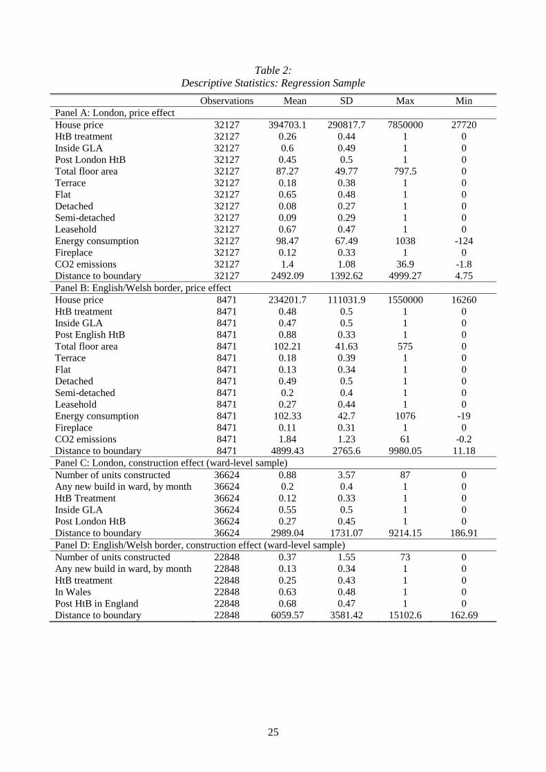
25

Table 2:

Descriptive Statistics: Regression Sample

Observations Mean SD Max Min

Panel A: London, price effect

House price 32127 394703.1 290817.7 7850000 27720

HtB treatment 32127 0.26 0.44 1 0

Inside GLA 32127 0.6 0.49 1 0

Post London HtB 32127 0.45 0.5 1 0

Total floor area 32127 87.27 49.77 797.5 0

Terrace 32127 0.18 0.38 1 0

Flat 32127 0.65 0.48 1 0

Detached 32127 0.08 0.27 1 0

Semi-detached 32127 0.09 0.29 1 0

Leasehold 32127 0.67 0.47 1 0

Energy consumption 32127 98.47 67.49 1038 -124

Fireplace 32127 0.12 0.33 1 0

CO2 emissions 32127 1.4 1.08 36.9 -1.8

Distance to boundary 32127 2492.09 1392.62 4999.27 4.75

Panel B: English/Welsh border, price effect

House price 8471 234201.7 111031.9 1550000 16260

HtB treatment 8471 0.48 0.5 1 0

Inside GLA 8471 0.47 0.5 1 0

Post English HtB 8471 0.88 0.33 1 0

Total floor area 8471 102.21 41.63 575 0

Terrace 8471 0.18 0.39 1 0

Flat 8471 0.13 0.34 1 0

Detached 8471 0.49 0.5 1 0

Semi-detached 8471 0.2 0.4 1 0

Leasehold 8471 0.27 0.44 1 0

Energy consumption 8471 102.33 42.7 1076 -19

Fireplace 8471 0.11 0.31 1 0

CO2 emissions 8471 1.84 1.23 61 -0.2

Distance to boundary 8471 4899.43 2765.6 9980.05 11.18

Panel C: London, construction effect (ward-level sample)

Number of units constructed 36624 0.88 3.57 87 0

Any new build in ward, by month 36624 0.2 0.4 1 0

HtB Treatment 36624 0.12 0.33 1 0

Inside GLA 36624 0.55 0.5 1 0

Post London HtB 36624 0.27 0.45 1 0

Distance to boundary 36624 2989.04 1731.07 9214.15 186.91

Panel D: English/Welsh border, construction effect (ward-level sample)

Number of units constructed 22848 0.37 1.55 73 0

Any new build in ward, by month 22848 0.13 0.34 1 0

HtB treatment 22848 0.25 0.43 1 0

In Wales 22848 0.63 0.48 1 0

Post HtB in England 22848 0.68 0.47 1 0

Distance to boundary 22848 6059.57 3581.42 15102.6 162.69

26

Table 3:

Supply Constraints Measures and Implied Price-Earnings Elasticities

Table 4:

Price Effect at GLA Boundary

Specifications (1) (2) (3) (4) (5)

HtB 1) 0.1613*** 0.0712*** 0.0446* 0.0641*** 0.0599**

(0.0423) (0.0261) (0.0245) (0.0232) (0.0241)

Year-month fixed

effects

Yes Yes Yes Yes Yes

Distance to boundary

on each side

Yes Yes Yes Yes Yes

Housing controls 2) No Yes Yes Yes Yes

Postcode FEs No No Yes Yes Yes

Census variables by

year 3)

No No No Yes Yes

Distance by year No No No No Yes

N 32127 32127 32127 32127 32127

R2 0.0906 0.6232 0.9187 0.9191 0.9192

Notes: 1) HtB captures the difference between the 40% and the 20% equity loan threshold (inside vs.

outside GLA). 2) Housing controls include total floor area, dwelling type, the tenure of properties,

whether the property has a fireplace, energy consumption and CO2 consumption. 3)

Neighborhood

controls (from the 2011 Census) are the percentage of (1) married residents and (2) residents with level-

4 and above educational qualifications at LSOA level.

Region English/Welsh

border

GLA

boundary

Greater Manchester

boundary

Share of land in green belts 3.77% 66.5% 52.6%

Average refusal rate 1979-2008 27.2% 35.6% 25.1%

Average share of developed land 6.3% 27.6% 18.2%

Average elevation range 476.0 143.9 382.3

Implied price-earning elasticity (OLS) 0.252 0.403 0.284

Implied price-earning elasticity (IV) 0.127 0.205 0.164

Notes: The refusal rate, share developed land and elevation range are weighted by the surface area of the Local

Planning Authority. Data on refusal rates, share developed land and elevation range come from Hilber and

Vermeulen (2016). The green belt shape file comes from the Ministry of Housing, Communities and Local

Government.

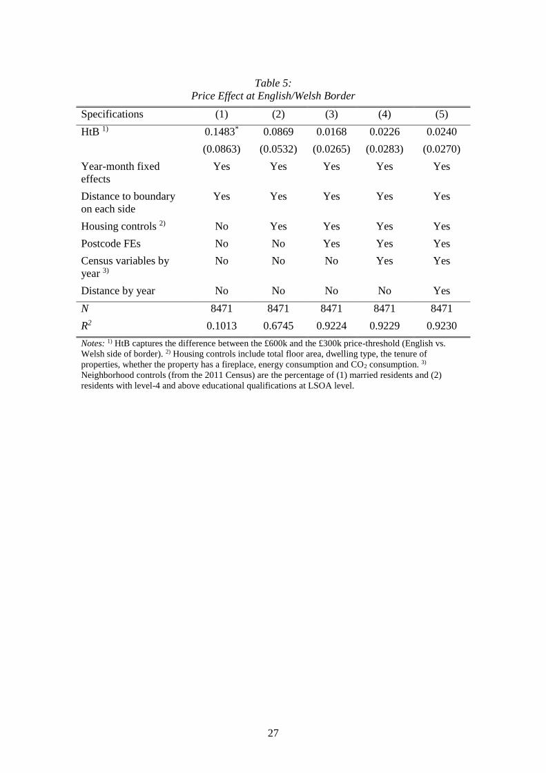
27

Table 5:

Price Effect at English/Welsh Border

Specifications (1) (2) (3) (4) (5)

HtB 1) 0.1483* 0.0869 0.0168 0.0226 0.0240

(0.0863) (0.0532) (0.0265) (0.0283) (0.0270)

Year-month fixed

effects

Yes Yes Yes Yes Yes

Distance to boundary

on each side

Yes Yes Yes Yes Yes

Housing controls 2) No Yes Yes Yes Yes

Postcode FEs No No Yes Yes Yes

Census variables by

year 3)

No No No Yes Yes

Distance by year No No No No Yes

N 8471 8471 8471 8471 8471

R2 0.1013 0.6745 0.9224 0.9229 0.9230

Notes: 1) HtB captures the difference between the £600k and the £300k price-threshold (English vs.

Welsh side of border). 2) Housing controls include total floor area, dwelling type, the tenure of

properties, whether the property has a fireplace, energy consumption and CO2 consumption. 3)

Neighborhood controls (from the 2011 Census) are the percentage of (1) married residents and (2)

residents with level-4 and above educational qualifications at LSOA level.

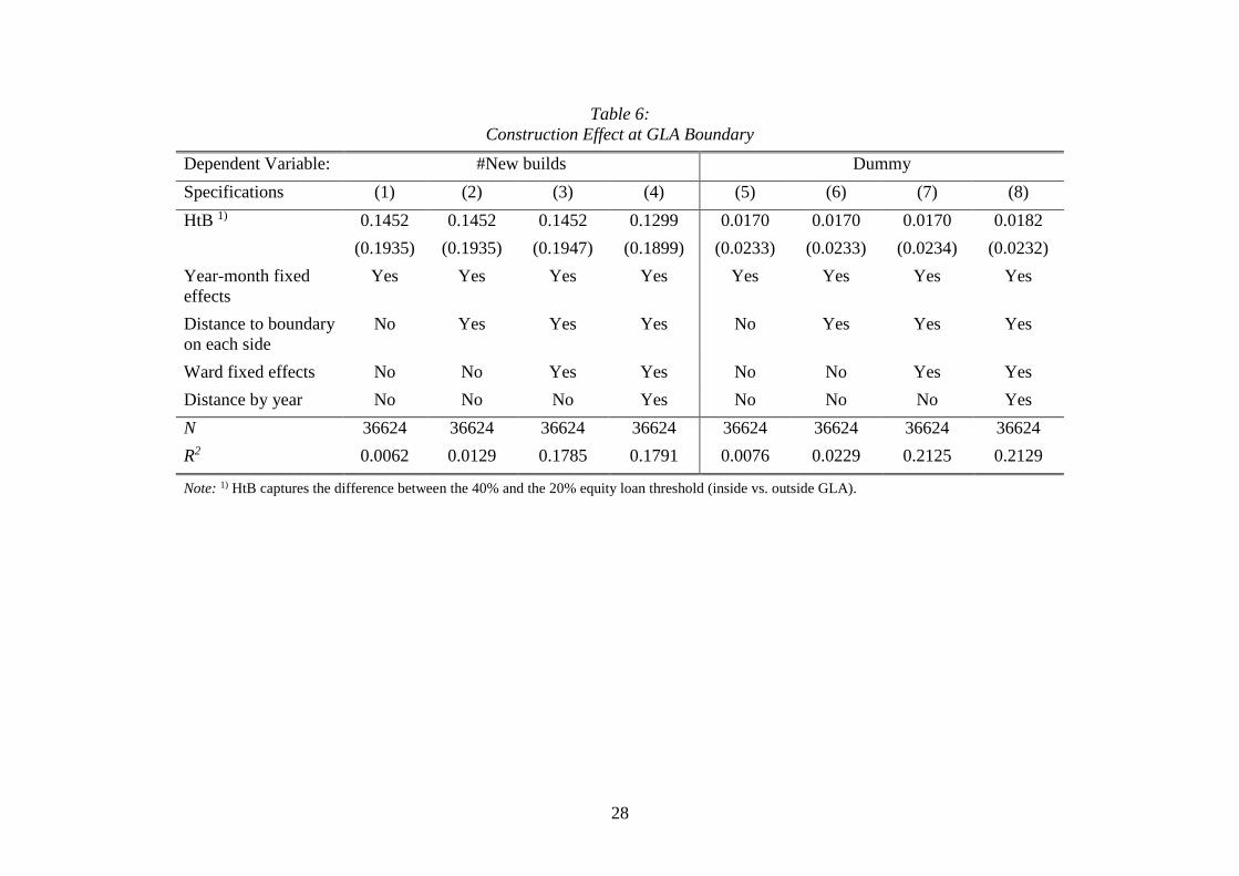
28

Table 6:

Construction Effect at GLA Boundary

Dependent Variable: #New builds Dummy

Specifications (1) (2) (3) (4) (5) (6) (7) (8)

HtB 1) 0.1452 0.1452 0.1452 0.1299 0.0170 0.0170 0.0170 0.0182

(0.1935) (0.1935) (0.1947) (0.1899) (0.0233) (0.0233) (0.0234) (0.0232)

Year-month fixed

effects

Yes Yes Yes Yes Yes Yes Yes Yes

Distance to boundary

on each side

No Yes Yes Yes No Yes Yes Yes

Ward fixed effects No No Yes Yes No No Yes Yes

Distance by year No No No Yes No No No Yes

N 36624 36624 36624 36624 36624 36624 36624 36624

R2 0.0062 0.0129 0.1785 0.1791 0.0076 0.0229 0.2125 0.2129

Note: 1) HtB captures the difference between the 40% and the 20% equity loan threshold (inside vs. outside GLA).

29

Table 7:

Construction Effect at English/Welsh Border

Dependent Variable: #New builds Dummy

Specifications (1) (2) (3) (4) (5) (6) (7) (8)

HtB 1) 0.3250*** 0.3250*** 0.3250*** 0.3549*** 0.0632** 0.0632** 0.0632** 0.0667***

(0.1043) (0.1043) (0.1049) (0.1046) (0.0249) (0.0249) (0.0251) (0.0248)

Year-month fixed

effects

Yes Yes Yes Yes Yes Yes Yes Yes

Distance to boundary

on each side

No Yes Yes Yes No Yes Yes Yes

Ward fixed effects No No Yes Yes No No Yes Yes

Distance by year No No No Yes No No No Yes

N 22848 22848 22848 22848 22848 22848 22848 22848

R2 0.0163 0.0271 0.2684 0.2696 0.0157 0.0382 0.2960 0.2969

Note: 1) HtB captures the difference between the £600k and the £300k price-threshold (English vs. Welsh side of border).

30

Table 8:

Effects on Financial Performance of Developers

Specifications (1) (2) (3) (4) (5)

Dependent Variable Ln(turnover) Ln(gross

profit)

Ln(net profit

before tax)

Ln((2)-

(3))

Ln(cost of

employees)

Panel A: HtB intensity sample

HtB intensity 1.1200** 1.4607** 2.4509* 0.8786** 0.9383***

× Post 1) (0.4168) (0.6219) (1.4252) (0.3222) (0.2875)

N 193 193 193 193 193

R2 0.9732 0.9651 0.8625 0.9059 0.9875

Panel B: DID sample

HtB dummy 0.4863*** 0.6781*** 1.5559*** 0.3045*** 0.4143***

× Post 2) (0.1510) (0.1900) (0.5577) (0.0889) (0.1346)

N 499 499 499 499 499

R2 0.9755 0.9733 0.8942 0.9458 0.9872

Year FEs Yes Yes Yes Yes Yes

Developer FEs Yes Yes Yes Yes Yes

Note: 1) HtB intensity is defined as the 5-year average ratio of HtB-completions relative to all completions. 2) HtB dummy

equals to one if a developer is involved in HtB business. Standard errors are clustered at developer level.

31

FIGURES

Fig. 1

New Builds near the Greater London Authority Boundary

Fig. 2

New Builds near English/Welsh Border

32

Fig. 3:

House Price Index at GLA boundary

Fig. 4:

House Price Index at English/Welsh Border

33

Fig. 5:

Boundary Discontinuity Design: Price Effect at GLA Boundary

Fig. 6:

Boundary Discontinuity Design: Price Effect at English/Welsh Border

34

Fig. 7:

Boundary Discontinuity Design: Construction Effect at GLA Boundary

Fig. 8:

Boundary Discontinuity Design: Construction Effect at English/Welsh Border

35

Fig. 9:

Developers’ Profits over Time

Fig. 10:

Histogram of House Prices in England

APPENDICES

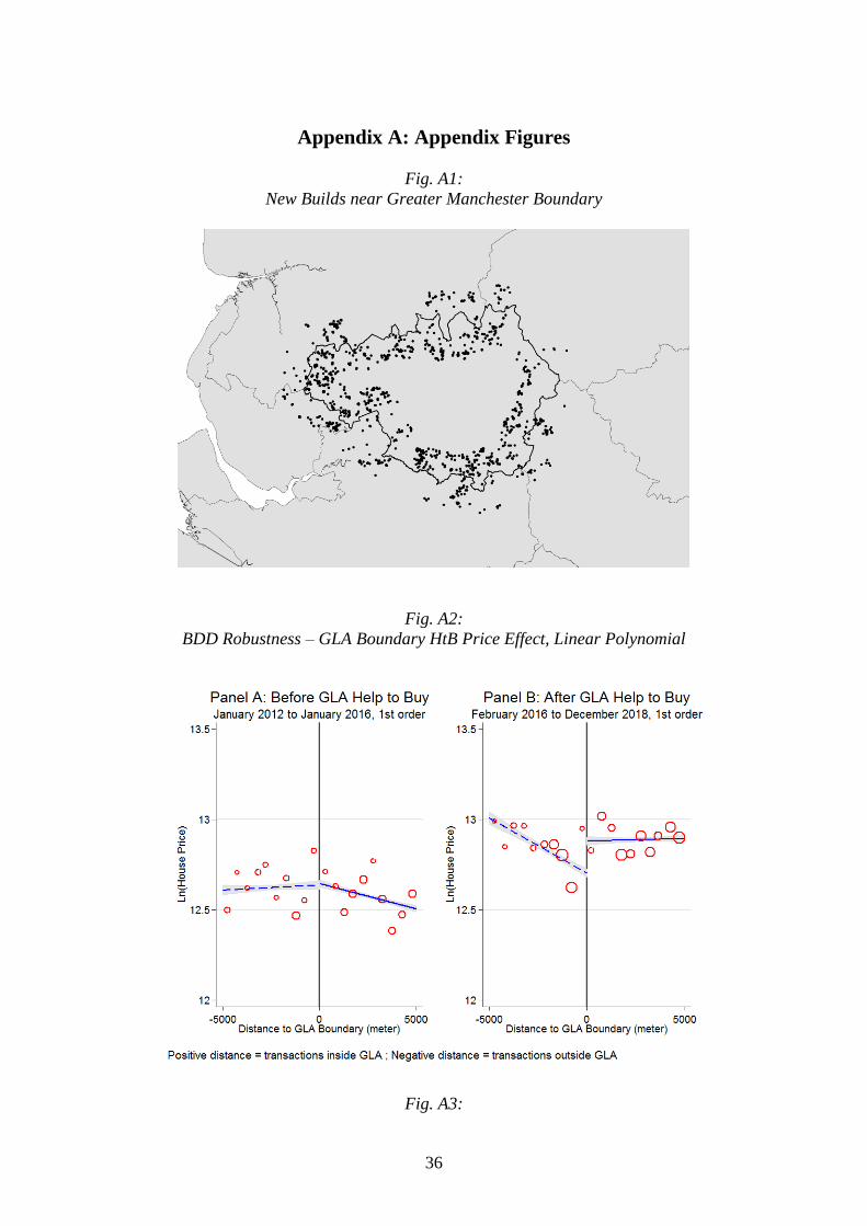
36

Appendix A: Appendix Figures

Fig. A1:

New Builds near Greater Manchester Boundary

Fig. A2:

BDD Robustness – GLA Boundary HtB Price Effect, Linear Polynomial

Fig. A3:

37

BDD Robustness – English/Welsh Border Price Effect, Linear Polynomial

Fig. A4:

Boundary Discontinuity Design: Placebo Manchester

Fig. A5:

38

Fraction of New Builds over Total Sales

Fig. A6:

The Fraction of New Builds over Total Sales

Fig. A7:

39

Estimated Bunching Effect

Fig. A8:

Size Effect at English/Welsh Border

40

Fig. A9:

Accumulated Help to Buy Completions (2013-2017)

41

Appendix B: Appendix Tables

Table B1:

Number of Transactions

London

5 km 4 km 3 km 2 km 1 km

Total number of sales 32127 25845 19850 14006 5149

Postcodes 1446 1250 948 634 246

Sales in treatment group 8495 6196 4596 2860 1108

Postcodes in treatment group 576 409 312 208 81

Wales

10 km 9 km 8 km 7 km 6 km

Total number of sales 8471 7612 6689 6204 5827

Postcodes 269 238 233 226 219

Sales in treatment group 4106 3527 3155 2960 2797

Postcodes in treatment group 171 142 138 132 125

Table B2:

Size Effect at English/Welsh Border (Units valued between £300-600k; 2011-2018)

Specifications (1) (2) (3) (4) (5)

HtB 1) -0.1198*** -0.0717* -0.0671* -0.0849*** -0.0673**

(0.0445) (0.0369) (0.0340) (0.0293) (0.0271)

Year-month fixed effects Yes Yes Yes Yes Yes

Distance to boundary Yes Yes Yes Yes Yes

Housing controls 2) No Yes Yes Yes Yes

Log house price No No Yes Yes Yes

Postcode district fixed effects No No No Yes Yes

Census variables by year 3) No No No No Yes

N 4763 4763 4763 4763 4763

R2 0.1553 0.6921 0.7631 0.8227 0.8301

Notes: 1) HtB captures the difference between the £600k and the £300k price-threshold (English vs. Welsh side of

border). We estimate using new build transactions valued between £300,000 and £600,000 within 20km from the

English/Welsh border from 2011 to 2018. We define ‘post HtB’ as starting from April 2014, which is one year

after the implementation of the English HtB. 2) Housing controls include dwelling type, the tenure of properties,

whether the property has a fireplace, energy consumption and CO2 consumption. 3) Neighborhood controls (from

the 2011 Census) are the percentage of (1) married residents and (2) residents with level-4 and above educational

qualifications at LSOA level. Standard errors are clustered at postcode district level.

42

Table B3:

Placebo Size Effect at English/Welsh Border (Units valued <£300k; 2011-2018)

Specifications (1) (2) (3) (4) (5)

HtB (placebo) 1) -0.0560 -0.0354 -0.0350 -0.0384 -0.0358

(0.0360) (0.0273) (0.0250) (0.0252) (0.0238)

Year-month fixed effects Yes Yes Yes Yes Yes

Distance to boundary Yes Yes Yes Yes Yes

Housing controls 2) No Yes Yes Yes Yes

Log house price No No Yes Yes Yes

Postcode district fixed effects No No No Yes Yes

Census variables by year 3) No No No No Yes

N 17640 17640 17640 17640 17640

R2 0.0798 0.6359 0.6872 0.7176 0.7208

Notes: 1) Placebo variable captures non-existing differences between the English and the Welsh side of the

border in (the generosity of) HtB for units valued below £300k. We estimate using new build transactions

valued less than £300,000 within 20km from the English/Welsh border from 2011 to 2018. We define ‘post

HtB’ as starting from April 2014, which is one year after the implementation of the English HtB. 2) Housing

controls include dwelling type, the tenure of properties, whether the property has a fireplace, energy

consumption and CO2 consumption. 3) Neighborhood controls (from the 2011 Census) are the percentage

of (1) married residents and (2) residents with level-4 and above educational qualifications at LSOA level.

Standard errors are clustered at postcode district level.

Table B4:

Placebo Size Effect at English/Welsh Border

(Units valued between £300-600k; 2010-2014)

Specifications (1) (2) (3) (4) (5)

HtB (placebo) 1) -0.1236* -0.0283 -0.0325 -0.0509 -0.0483

(0.0723) (0.0557) (0.0564) (0.0455) (0.0513)

Year-month fixed effects Yes Yes Yes Yes Yes

Distance to boundary Yes Yes Yes Yes Yes

Housing controls 2) No Yes Yes Yes Yes

Log house price No No Yes Yes Yes

Postcode district fixed effects No No No Yes Yes

Census variables by year 3) No No No No Yes

N 1275 1275 1275 1275 1275

R2 0.1163 0.5561 0.6261 0.7375 0.7407

Notes: 1) Placebo variable captures non-existing differences between the English and the Welsh side of the

border for time prior to 2015. We estimate using new build transactions valued between £300,000 and

£600,000 within 20km away from the English/Welsh border from 2010 to 2014. We define year 2013 and

2014 as post HtB period. 2) Housing controls include dwelling type, the tenure of properties, whether the

property has a fireplace, energy consumption and CO2 consumption. 3) Neighborhood controls (from the

2011 Census) are the percentage of (1) married residents and (2) residents with level-4 and above

educational qualifications at LSOA level. Standard errors are clustered at postcode district level.

43

Table B5:

Effects on Mortgage Origination Inside of GLA Boundary

Specifications (1) (2) (3) (4) (5)

HtB 1) -0.0014 -0.0014 -0.0014 -0.0014 -0.0016

(0.0080) (0.0080) (0.0080) (0.0082) (0.0083)

Year-quarter fixed effects Yes Yes Yes Yes Yes

Distance to boundary No Yes Yes Yes Yes

Postcode area fixed effects No No Yes No No

Postcode sector fixed effects No No No Yes Yes

Distance by year No No No No Yes

N 10836 10836 10836 10836 10836

R2 0.0191 0.0206 0.1876 0.9955 0.9955

Note: 1) HtB captures the difference between the 40% and the 20% equity loan threshold (inside vs.

outside GLA).

Table B6:

Robustness – Bandwidth Selection & Price Effect at GLA Boundary

Specifications (1) (2) (3) (4) (5)

Panel A: 2.5 km Bandwidth

HtB 1) 0.1044* 0.0413 0.0436* 0.0602** 0.0432*

(0.0548) (0.0330) (0.0262) (0.0276) (0.0245)

N 17005 17005 17005 17005 17005

Panel B: 7.5 km Bandwidth

HtB 1) 0.1243*** 0.0745*** 0.0457** 0.0550** 0.0546**

(0.0352) (0.0218) (0.0219) (0.0248) (0.0248)

N 51079 51079 51079 51079 51079

Year-month FEs Yes Yes Yes Yes Yes

Distance to boundary Yes Yes Yes Yes Yes

Housing controls 2) No Yes Yes Yes Yes

Postcode FEs No No Yes Yes Yes

Census variables by year 3) No No No Yes Yes

Distance by year No No No No Yes

Notes: 1) - 3) see Table 4.

44

Table B7:

Robustness – Bandwidth Selection & Price Effect at English/Welsh Border

Specifications (1) (2) (3) (4) (5)

Panel A: 5 km Bandwidth

HtB 0.0207 -0.0379 0.0182 0.0278 0.0228

(0.0879) (0.0447) (0.0280) (0.0307) (0.0315)

N 4864 4864 4864 4864 4864

Panel B: 15 km Bandwidth

HtB 0.1496** 0.0810** -0.0064 -0.0027 -0.0029

(0.0635) (0.0386) (0.0194) (0.0205) (0.0206)

N 14496 14496 14496 14496 14496

Year-month FEs Yes Yes Yes Yes Yes

Distance to boundary Yes Yes Yes Yes Yes

Housing controls 2) No Yes Yes Yes Yes

Postcode FEs No No Yes Yes Yes

Census variables by year 3) No No No Yes Yes

Distance by year No No No No Yes

Notes: 1) - 3) see Table 5.

Table B8:

Placebo - Price Effect at Greater Manchester Boundary

Specifications (1) (2) (3) (4) (5)

HtB (placebo) 1) 0.0451 0.0151 -0.0035 -0.0056 -0.0047

(0.0570) (0.0344) (0.0183) (0.0184) (0.0179)

Year-month fixed effects Yes Yes Yes Yes Yes

Distance to boundary Yes Yes Yes Yes Yes

Housing controls 2) No Yes Yes Yes Yes

Postcode fixed effects No No Yes Yes Yes

Census variables by year 3) No No No Yes Yes

Distance by year No No No No Yes

N 13318 13318 13318 13318 13318

R2 0.0874 0.6767 0.9221 0.9223 0.9224

Notes: 1) Placebo variable captures non-existing differences between inside and outside the Greater

Manchester boundary in the generosity of HtB. 2) Housing controls include total floor area, dwelling type,

the tenure of properties, whether the property has a fireplace, energy consumption and CO2 consumption. 3)

Neighborhood controls (from the 2011 Census) are the percentage of (1) married residents and (2)

residents with level-4 and above educational qualifications at LSOA level.

45

Table B9:

Price Effect at GLA Boundary – Donut Approach

Keep new build transactions between …

Specifications 0.5-5km 1- 5 km 1.5 - 5 km

HtB 1) 0.0632** 0.0685** 0.0836***

(0.0249) (0.0274) (0.0292)

Year-month fixed effects Yes Yes Yes

Distance to boundary Yes Yes Yes

Housing controls 2) Yes Yes Yes

Postcode FEs Yes Yes Yes

Census variables by year 3) Yes Yes Yes

Distance by year Yes Yes Yes

N 30170 26978 22682

R2 0.9167 0.9146 0.9085

Notes: 1) HtB captures the difference between the 40% and the 20% equity loan threshold (inside vs.

outside GLA). 2) Housing controls include total floor area, dwelling type, the tenure of properties,

whether the property has a fireplace, energy consumption and CO2 consumption. 3)

Neighborhood

controls (from the 2011 Census) are the percentage of (1) married residents and (2) residents with level-

4 and above educational qualifications at LSOA level.

46

Table B10:

Robustness – GLA Boundary Contemporaneous Construction Effects

Dependent

Variable:

#New builds Dummy

Specifications (1) (2) (3) (4) (5) (6) (7) (8)

HtB 1) 0.0445 0.0445 0.0445 0.0238 0.0113 0.0113 0.0113 0.0116

(0.1682) (0.1682) (0.1692) (0.1659) (0.0231) (0.0231) (0.0233) (0.0232)

Year-month

fixed effects

Yes Yes Yes Yes Yes Yes Yes Yes

Distance to

boundary

No Yes Yes Yes No Yes Yes Yes

Ward fixed

effects

No No Yes Yes No No Yes Yes

Distance by

year

No No No Yes No No No Yes

N 36624 36624 36624 36624 36624 36624 36624 36624

R2 0.0062 0.0129 0.1784 0.1791 0.0075 0.0229 0.2125 0.2129

Note: 1) HtB captures the difference between the 40% and the 20% equity loan threshold (inside vs. outside GLA).

Table B11:

Robustness - English/Welsh Border Contemporaneous Construction Effects

Dependent

Variable:

#New builds Dummy

Specifications (1) (2) (3) (4) (5) (6) (7) (8)

HtB 0.3147*** 0.3147*** 0.3147*** 0.3448*** 0.0630*** 0.0630*** 0.0630*** 0.0664***

(0.1052) (0.1052) (0.1058) (0.1074) (0.0234) (0.0234) (0.0236) (0.0236)

Year-month

fixed effects

Yes Yes Yes Yes Yes Yes Yes Yes

Distance to

boundary

No Yes Yes Yes No Yes Yes Yes

Ward FEs No No Yes Yes No No Yes Yes

Distance by

year

No No No Yes No No No Yes

N 22848 22848 22848 22848 22848 22848 22848 22848

R2 0.0155 0.0263 0.2676 0.2687 0.0151 0.0377 0.2954 0.2963

Note: 1) HtB captures the difference between the £600k and the £300k price-threshold (English vs. Welsh side of border).

47

Table B12:

Placebo - Construction Effect at Greater Manchester Boundary

Dependent

Variable:

#New builds Dummy

Specifications (1) (2) (3) (4) (5) (6) (7) (8)

HtB (placebo) 1) -0.1769 -0.1769 -0.1769 -0.1693 0.02 0.02 0.02 0.0176

(0.2122) (0.2122) (0.2135) (0.2107) (0.0406) (0.0406) (0.0409) (0.0406)

Year-month

fixed effects

Yes Yes Yes Yes Yes Yes Yes Yes

Distance to

boundary

No Yes Yes Yes No Yes Yes Yes

Ward fixed

effects

No No Yes Yes No No Yes Yes

Distance by

year

No No No Yes No No No Yes

N 17808 17808 17808 17808 17808 17808 17808 17808

R2 0.0277 0.0401 0.2339 0.2342 0.0236 0.0539 0.3343 0.3345

Note: 1) Placebo variable captures non-existing differences between inside and outside the Greater Manchester boundary in the

generosity of HtB.

Table B13:

Price Effect at English/Welsh Border

(Pre-period: January 2012 to March 2013; Post period: January 2014 to December 2018)

Specifications (1) (2) (3) (4) (5)

HtB 1) 0.1405 0.0840 0.0271 0.0291 0.0308

(0.0909) (0.0566) (0.0372) (0.0413) (0.0412)

Year-month fixed

effects

Yes Yes Yes Yes Yes

Distance to boundary Yes Yes Yes Yes Yes

Housing controls 2) No Yes Yes Yes Yes

Postcode FEs No No Yes Yes Yes

Census variables by

year 3)

No No No Yes Yes

Distance by year No No No No Yes

N 7660 7660 7660 7660 7660

R2 0.0983 0.6787 0.9225 0.9230 0.9232

Notes: 1) HtB captures the difference between the £600k and the £300k price-threshold (English vs.

Welsh side of border). 2) Housing controls include total floor area, dwelling type, the tenure of

properties, whether the property has a fireplace, energy consumption and CO2 consumption. 3)

Neighborhood controls (from the 2011 Census) are the percentage of (1) married residents and (2)

residents with level-4 and above educational qualifications at LSOA level.

48

Table B14:

Construction Effect at English/Welsh Border

(Pre-period: January 2012 to March 2013; Post period: January 2015 to December 2018)

Dependent

Variable:

#New builds Dummy

Specifications (1) (2) (3) (4) (5) (6) (7) (8)

HtB 1) 0.3991*** 0.3991*** 0.3991*** 0.4379*** 0.0768*** 0.0768*** 0.0768*** 0.0814***

(0.1286) (0.1286) (0.1296) (0.1317) (0.0282) (0.0282) (0.0284) (0.0285)

Year-month FEs Yes Yes Yes Yes Yes Yes Yes Yes

Distance to

boundary

No Yes Yes Yes No Yes Yes Yes

Ward fixed

effects

No No Yes Yes No No Yes Yes

Distance by year No No No Yes No No No Yes

N 17136 17136 17136 17136 17136 17136 17136 17136

R2 0.0182 0.0291 0.2668 0.2682 0.0185 0.0424 0.3045 0.3057

Note: 1) HtB captures the difference between the £600k and the £300k price-threshold (English vs. Welsh side of border).

Table B15:

Back-of-the-Envelope Calculation

Year

HtB

interest

Mortgage

Rate

Net Interest

Subsidy

Difference of

Equity Loan

Present

Value

1 0.00% 2.74% 2.74% 20.00% 0.54%

2 0.00% 2.74% 2.74% 20.00% 0.53%

3 0.00% 2.74% 2.74% 20.00% 0.53%

4 0.00% 2.74% 2.74% 20.00% 0.52%

5 0.00% 2.74% 2.74% 20.00% 0.51%

6 1.75% 2.74% 0.99% 20.00% 0.18%

7 1.81% 2.74% 0.93% 20.00% 0.17%

8 1.86% 2.74% 0.88% 20.00% 0.15%

9 1.92% 2.74% 0.82% 20.00% 0.13%

10 1.98% 2.74% 0.76% 20.00% -1.70%

Sum 1.56%