Example 17 - دچينې ويب ... · Example 17.3 Analyse the rigid ... In this lesson, ... Module...

Example 17.3

Analyse the rigid frame shown in Fig. 17.5 a. Moment of inertia of all the members are shown in the figure. Draw bending moment diagram.

Under the action of external forces, the frame gets deformed as shown in Fig. 17.5b. In this figure, chord to the elastic curve are shown by dotted line. 'BB is perpendicular to AB and is perpendicular to . The chords to the elastic "CC DC

Version 2 CE IIT, Kharagpur

curve "AB rotates by an angle AB , rotates by ""CB BC and rotates by DC

CD as shown in figure. Due to symmetry, ABCD ! . From the geometry of the

figure,

ABAB

ABLL

BB 1" "#!!

But

$cos1

"!"

Thus,

5cos

"#!

"#!

$

AB

ABL

5

"#!CD

5tan

2

tan2

2

2 "!"!

"!

"! $

$ BC (1)

We have three independent unknowns for this problem CB %% , and . The ends "

A and are fixed. Hence, D .0!! DA %% Fixed end moments are,

.0;0;.50.2;.50.2;0;0 !!#!&!!! F

DC

F

CD

F

CB

F

BC

F

BA

F

AB MMmkNMmkNMMM

Now, writing the slope-deflection equations for the six beam end moments,

' (ABAAB

IEM % 3

1.5

)2(2#!

"&! EIEIM BAB 471.0784.0 %

"&! EIEIM BBA 471.0568.1 %

"#&&! EIEIEIM CBBC 6.025.2 %%

"#&&#! EIEIEIM CBBC 6.025.2 %%

"&! EIEIM CCD 471.0568.1 %

"&! EIEIM CDC 471.0784.0 % (2)

Now, considering the joint equilibrium of B andC , yields


00 !&)!* BCBAB MMM

5.2129.0568.3 #!"#& EIEIEI CB %% (3)

00 !&)!* CDCBC MMM

5.2129.0568.3 !"#& EIEIEI BC %% (4)

Shear equation for Column AB

0)1(5 11 !&## VMMH BAAB (5)

Column CD

0)1(5 22 !&## VMMH DCCD (6)

Beam BC

01020 1 !###!* CBBCC MMVM (7)


* !&! 50 21 HHFX (8)

* !##! 0100 21 VVFY (9)

From equation (7), 2

101

&&! CBBC MM

V

From equation (8), 21 5 HH #!

From equation (9), 102

101012 #

&&!#! CBBC MM

VV

Substituting the values of and in equations (5) and (6), 11,HV 2V

0221060 2 !&&### CBBCBAAB MMMMH (10)

0221010 2 !&&##&# CBBCDCCD MMMMH (11)

Eliminating in equation (10) and (11), 2H

25!##&&& CBBCDCCDBAAB MMMMMM (12)

Substituting the values of in (12) we get the required third

equation. Thus,

DCCDBAAB MMMM ,,,

&"& EIEI B 471.0784.0 % &"& EIEI B 471.0568.1 % &"& EIEI C 471.0568.1 %

"& EIEI C 471.0784.0 % -( "#&& EIEIEI CB 6.025.2 %% )-

( "#&&# EIEIEI CB 6.025.2 %% ) 25!

Simplifying,

25084.3648.0648.0 !"&## EIEIEI BC %% (13)

Solving simultaneously equations (3) (4) and (13), yields

205.1;741.0 !#! CB EIEI %% and 204.8!"EI .

Substituting the values of CB EIEI %% , and "EI in the slope-deflection equation

(3), one could calculate beam end moments. Thus,

3.28 kN.mABM !


2.70 kN.mBAM !

2.70 kN.mBCM ! #

5.75 kN.mCBM ! #

5.75 kN.mCDM !

4.81 kN.mDCM ! . (14)

The bending moment diagram for the frame is shown in Fig. 17.5 d.

Summary

In this lesson, slope-deflection equations are derived for the plane frame undergoing sidesway. Using these equations, plane frames with sidesway are analysed. The reactions are calculated from static equilibrium equations. A couple of problems are solved to make things clear. In each numerical example, the bending moment diagram is drawn and deflected shape is sketched for the plane frame.


Module 3

Analysis of Statically Indeterminate

Structures by the Displacement Method


Lesson 18

The Moment-Distribution Method:

Introduction Version 2 CE IIT, Kharagpur

Instructional Objectives

After reading this chapter the student will be able to 1. Calculate stiffness factors and distribution factors for various members in

a continuous beam. 2. Define unbalanced moment at a rigid joint. 3. Compute distribution moment and carry-over moment. 4. Derive expressions for distribution moment, carry-over moments. 5. Analyse continuous beam by the moment-distribution method.

18.1 Introduction

In the previous lesson we discussed the slope-deflection method. In slope-deflection analysis, the unknown displacements (rotations and translations) are related to the applied loading on the structure. The slope-deflection method results in a set of simultaneous equations of unknown displacements. The number of simultaneous equations will be equal to the number of unknowns to be evaluated. Thus one needs to solve these simultaneous equations to obtain displacements and beam end moments. Today, simultaneous equations could be solved very easily using a computer. Before the advent of electronic computing, this really posed a problem as the number of equations in the case of multistory building is quite large. The moment-distribution method proposed by Hardy Cross in 1932, actually solves these equations by the method of successive approximations. In this method, the results may be obtained to any desired degree of accuracy. Until recently, the moment-distribution method was very popular among engineers. It is very simple and is being used even today for preliminary analysis of small structures. It is still being taught in the classroom for the simplicity and physical insight it gives to the analyst even though stiffness method is being used more and more. Had the computers not emerged on the scene, the moment-distribution method could have turned out to be a very popular method. In this lesson, first moment-distribution method is developed for continuous beams with unyielding supports.

18.2 Basic Concepts

In moment-distribution method, counterclockwise beam end moments are taken as positive. The counterclockwise beam end moments produce clockwise moments on the joint Consider a continuous beam ABCD as shown in Fig.18.1a.

In this beam, ends A and D are fixed and hence, 0 DA !! .Thus, the

deformation of this beam is completely defined by rotations B! and C! at joints B

and C respectively. The required equation to evaluate B! andC! is obtained by

considering equilibrium of joints B and C. Hence,


0 " BM # 0 $ BCBA MM (18.1a)

0 " CM # 0 $ CDCB MM (18.1b)

According to slope-deflection equation, the beam end moments are written as

)2(2

B

AB

ABF

BABAL

EIMM !$

AB

AB

L

EI4 is known as stiffness factor for the beam AB and it is denoted

by . is the fixed end moment at joint B of beam AB when joint B is fixed.

Thus,

ABkFBAM

BAB

F

BABA KMM !$

%%&

'(()

*$$

2

CBBC

FBCBC KMM

!!

%%&

'(()

*$$

2

BCCB

FCBCB KMM

!!

CCDFCDCD KMM !$ (18.2)

In Fig.18.1b, the counterclockwise beam-end moments and produce

a clockwise moment on the joint as shown in Fig.18.1b. To start with, in

moment-distribution method, it is assumed that joints are locked i.e. joints are prevented from rotating. In such a case (vide Fig.18.1b),

BAM BCM

BM

0 CB !! , and hence

FBABA MM FBCBC MM FCBCB MM FCDCD MM (18.3)

Since joints B and C are artificially held locked, the resultant moment at joints B

and C will not be equal to zero. This moment is denoted by and is known as

the unbalanced moment.

BM


Thus,FBC

FBAB MMM $

In reality joints are not locked. Joints B and C do rotate under external loads. When the joint B is unlocked, it will rotate under the action of unbalanced

moment . Let the joint B rotate by an angleBM 1B! , under the action of . This

will deform the structure as shown in Fig.18.1d and introduces distributed

moment in the span BA and BC respectively as shown in the figure.

The unknown distributed moments are assumed to be positive and hence act in counterclockwise direction. The unbalanced moment is the algebraic sum of the fixed end moments and act on the joint in the clockwise direction. The unbalanced moment restores the equilibrium of the joint B. Thus,

BM

dBC

dBA MM ,

,0 " BM (18.4) 0 $$ BdBC

dBA MMM

The distributed moments are related to the rotation 1B! by the slope-deflection

equation.


1BBAdBA KM !

1BBCdBC KM ! (18.5)

Substituting equation (18.5) in (18.4), yields

+ , BBCBAB MKK - $1!

BCBA

BB

KK

M

$- 1!

In general,

"-

K

M BB1! (18.6)

where summation is taken over all the members meeting at that particular joint. Substituting the value of 1B! in equation (18.5), distributed moments are

calculated. Thus,

BBAd

BA MK

KM

"-

BBCd

BC MK

KM

"- (18.7)

The ratio "K

K BAis known as the distribution factor and is represented by .BADF

Thus,

BBAdBA MDFM .-

BBCdBC MDFM .- (18.8)

The distribution moments developed in a member meeting at B, when the joint B

is unlocked and allowed to rotate under the action of unbalanced moment is

equal to a distribution factor times the unbalanced moment with its sign reversed.

BM

As the joint B rotates under the action of the unbalanced moment, beam end moments are developed at ends of members meeting at that joint and are known as distributed moments. As the joint B rotates, it bends the beam and beam end moments at the far ends (i.e. at A and C) are developed. They are known as carry over moments. Now consider the beam BC of continuous beam ABCD.


When the joint B is unlocked, joint C is locked .The joint B rotates by 1B! under

the action of unbalanced moment (vide Fig. 18.1e). Now from slope-

deflection equations

BM

BBCdBC KM !

BBCBC KM !2

1

1

2

d

CB BCM M (18.9)

The carry over moment is one half of the distributed moment and has the same sign. With the above discussion, we are in a position to apply moment-distribution method to statically indeterminate beam. Few problems are solved here to illustrate the procedure. Carefully go through the first problem, wherein the moment-distribution method is explained in detail.

Example 18.1

A continuous prismatic beam ABC (see Fig.18.2a) of constant moment of inertia is carrying a uniformly distributed load of 2 kN/m in addition to a concentrated load of 10 kN. Draw bending moment diagram. Assume that supports are unyielding.


SolutionAssuming that supports B and C are locked, calculate fixed end moments developed in the beam due to externally applied load. Note that counterclockwise moments are taken as positive.

2 2 91.5 kN.m

12 12

F ABAB

wLM

.

2 2 91.5 kN.m

12 12

F ABBA

wLM

. - - -

2

2

10 2 45 kN.m

16

F

BC

BC

PabM

L

. .

2

2

10 2 45 kN.m

16

F

CB

BC

Pa bM

L

. . - - - (1)

Before we start analyzing the beam by moment-distribution method, it is required to calculate stiffness and distribution factors.

3

4EIK BA

4

4EIK BC

At B: " EIK 333.2

571.0333.2

333.1

EI

EIDFBA

429.0333.2

EI

EIDFBC


At C: " EIK

0.1 CBDF

Note that distribution factor is dimensionless. The sum of distribution factor at a joint, except when it is fixed is always equal to one. The distribution moments are developed only when the joints rotate under the action of unbalanced moment. In the case of fixed joint, it does not rotate and hence no distribution moments are developed and consequently distribution factor is equal to zero. In Fig.18.2b the fixed end moments and distribution factors are shown on a working diagram. In this diagram B and C are assumed to be locked.

Now unlock the joint C. Note that joint C starts rotating under the unbalanced moment of 5 kN.m (counterclockwise) till a moment of -5 kN.m is developed (clockwise) at the joint. This in turn develops a beam end moment of +5 kN.m

. This is the distributed moment and thus restores equilibrium. Now joint C

is relocked and a line is drawn below +5 kN.m to indicate equilibrium. When joint C rotates, a carry over moment of +2.5 kN.m is developed at the B end of member BC.These are shown in Fig.18.2c.

+ CBM ,

When joint B is unlocked, it will rotate under an unbalanced moment equal to algebraic sum of the fixed end moments(+5.0 and -1.5 kN.m) and a carry over moment of +2.5 kN.m till distributed moments are developed to restore equilibrium. The unbalanced moment is 6 kN.m. Now the distributed moments

and are obtained by multiplying the unbalanced moment with the

corresponding distribution factors and reversing the sign. Thus, BCM BAM


574.2- BCM kN.m and 426.3- BAM kN.m. These distributed moments restore

the equilibrium of joint B. Lock the joint B. This is shown in Fig.18.2d along with the carry over moments.

Now, it is seen that joint B is balanced. However joint C is not balanced due to the carry over moment -1.287 kN.m that is developed when the joint B is allowed to rotate. The whole procedure of locking and unlocking the joints C and Bsuccessively has to be continued till both joints B and C are balanced simultaneously. The complete procedure is shown in Fig.18.2e.

The iteration procedure is terminated when the change in beam end moments is less than say 1%. In the above problem the convergence may be improved if we leave the hinged end C unlocked after the first cycle. This will be discussed in the next section. In such a case the stiffness of beam BC gets modified. The above calculations can also be done conveniently in a tabular form as shown in Table 18.1. However the above working method is preferred in this course.


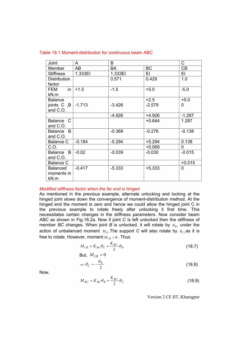
Table 18.1 Moment-distribution for continuous beam ABC

Joint A B C

Member AB BA BC CB

Stiffness 1.333EI 1.333EI EI EI

Distribution factor

0.571 0.429 1.0

FEM in kN.m

+1.5 -1.5 +5.0 -5.0

Balancejoints C ,B and C.O.

-1.713 -3.426+2.5-2.579

+5.00

-4.926 +4.926 -1.287

Balance C and C.O.

+0.644 1.287

Balance B and C.O.

-0.368 -0.276 -0.138

Balance C -0.184 -5.294 +5.294 0.138

C.O. +0.069 0

Balance B and C.O.

-0.02 -0.039 -0.030 -0.015

Balance C +0.015

Balancedmoments in kN.m

-0.417 -5.333 +5.333 0

Modified stiffness factor when the far end is hinged As mentioned in the previous example, alternate unlocking and locking at the hinged joint slows down the convergence of moment-distribution method. At the hinged end the moment is zero and hence we could allow the hinged joint C in the previous example to rotate freely after unlocking it first time. This necessitates certain changes in the stiffness parameters. Now consider beam ABC as shown in Fig.18.2a. Now if joint C is left unlocked then the stiffness of member BC changes. When joint B is unlocked, it will rotate by 1B! under the

action of unbalanced moment .The support C will also rotate by BM 1C! as it is

free to rotate. However, moment 0 CBM . Thus

BBC

CBCCB

KKM !!

2$ (18.7)

But, 0 CBM

#2

BC

!! - (18.8)

Now,

CBC

BBCBC

KKM !!

2$ (18.9)


Substituting the value of C! in eqn. (18.9),

BBCBBC

BBCBC KK

KM !!!4

3

4 - (18.10)

BRBCBC KM ! (18.11)

The is known as the reduced stiffness factor and is equal to RBCK BCK

4

3

.Accordingly distribution factors also get modified. It must be noted that there is no carry over to joint C as it was left unlocked.

Example 18.2

Solve the previous example by making the necessary modification for hinged end C.

Fixed end moments are the same. Now calculate stiffness and distribution factors.

EIEIKEIK BCBA 75.04

3,333.1

Joint B: ," ,083.2K 64.0 FBAD 36.0 F

BCD

Joint C: " ,75.0 EIK 0.1 FCBD

All the calculations are shown in Fig.18.3a

Please note that the same results as obtained in the previous example are obtained here in only one cycle. All joints are in equilibrium when they are unlocked. Hence we could stop moment-distribution iteration, as there is no unbalanced moment anywhere.


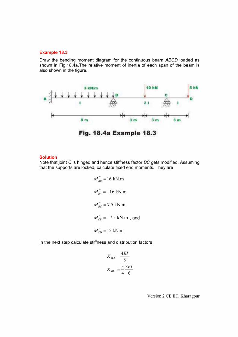
Example 18.3

Draw the bending moment diagram for the continuous beam ABCD loaded as shown in Fig.18.4a.The relative moment of inertia of each span of the beam is also shown in the figure.

SolutionNote that joint C is hinged and hence stiffness factor BC gets modified. Assuming that the supports are locked, calculate fixed end moments. They are

16 kN.mF

ABM

16 kN.mF

BAM -

7.5 kN.mF

BCM

7.5 kN.mF

CBM - , and

15 kN.mF

CDM

In the next step calculate stiffness and distribution factors

8

4EIK BA

6

8

4

3 EIK BC


6

8EIKCB

At joint B:

" $ EIEIEIK 5.10.15.0

0.50.333

1.5

F

BA

EID

EI

1.00.667

1.5

F

BC

EID

EI

At C:

0.1, " FCBDEIK

Now all the calculations are shown in Fig.18.4b

This problem has also been solved by slope-deflection method (see example 14.2).The bending moment diagram is shown in Fig.18.4c.


Summary

An introduction to the moment-distribution method is given here. The moment-distribution method actually solves these equations by the method of successive approximations. Various terms such as stiffness factor, distribution factor, unbalanced moment, distributing moment and carry-over-moment are defined in this lesson. Few problems are solved to illustrate the moment-distribution method as applied to continuous beams with unyielding supports.


MODULE

3

ANALYSIS OF

STATICALLY

INDETERMINATE

STRUCTURES BY THE

DISPLACEMENT

METHOD


LESSON

19

THE MOMENT-

DISTRIBUTION

METHOD: STATICALLY

INDETERMINATE

BEAMS WITHSUPPORT

SETTLEMENTS



After reading this chapter the student will be able to

1. Solve continuous beam with support settlements by the moment-

distribution method.

2. Compute reactions at the supports.

3. Draw bending moment and shear force diagrams.

4. Draw the deflected shape of the continuous beam.

19.1 Introduction

In the previous lesson, moment-distribution method was discussed in the context

of statically indeterminate beams with unyielding supports. It is very well known

that support may settle by unequal amount during the lifetime of the structure.

Such support settlements induce fixed end moments in the beams so as to hold

the end slopes of the members as zero (see Fig. 19.1).

In lesson 15, an expression (equation 15.5) for beam end moments were derived

by superposing the end moments developed due to

1. Externally applied loads on beams

2. Due to displacements BA , and ! (settlements).

The required equations are,

"#

$%&

' !())*

AB

BA

AB

ABF

ABABLL

EIMM

32

2 (19.1a)


!"

#$%

& '())*

AB

AB

AB

ABF

BABALL

EIMM

32

2 (19.1b)

This may be written as,

(19.2a) + , S

ABBAAB

F

ABAB MKMM )))* 22

+ ,2 2F

BA BA AB B A BA

SM M K M * ) ) ) (19.2b)

whereAB

ABAB

L

EIK * is the stiffness factor for the beam AB. The coefficient 4 has

been dropped since only relative values are required in calculating distribution

factors.

Note that 2

6

AB

ABS

BA

S

ABL

EIMM

'(** (19.3)

S

ABM is the beam end moments due to support settlement and is negative

(clockwise) for positive support settlements (upwards). In the moment-distribution

method, the support moments and due to uneven support settlements

are distributed in a similar manner as the fixed end moments, which were

described in details in lesson 18.

S

ABM S

BAM

It is important to follow consistent sign convention. Here counterclockwise beam

end moments are taken as positive and counterclockwise chord rotation -.

/01

2 'L

is

taken as positive. The moment-distribution method as applied to statically

indeterminate beams undergoing uneven support settlements is illustrated with a

few examples.


Example 19.1

Calculate the support moments of the continuous beam (Fig. 19.2a) having

constant flexural rigidity

ABC

EI throughout, due to vertical settlement of support B

by 5mm. Assume ; and .200 GPaE * 4 44 10 mI (* 3

Solution

There is no load on the beam and hence fixed end moments are zero. However,

fixed end moments are developed due to support settlement of B by 5mm. In the

span AB , the chord rotates by AB4 in clockwise direction. Thus,

5

105 3(3(*AB4

--.

/001

2 3(

3333(*(**

((

5

105

5

1041020066 349

AB

AB

ABS

BA

S

ABL

EIMM 4

96000 Nm 96 kNm.* * (1)

In the span , the chord rotates by BC BC4 in the counterclockwise direction and

hence taken as positive.

5

105 3(3*BC4


--.

/001

2 33333(*(**

((

5

105

5

1041020066 349

BC

BC

BCS

CB

S

BCL

EIMM 4

.9696000 kNmNm (*(* (2)

Now calculate stiffness and distribution factors.

EIL

EIK

AB

ABBA 2.0** and EI

L

EIK

BC

BCBC 15.0

4

3** (3)

Note that, while calculating stiffness factor, the coefficient 4 has been dropped

since only relative values are required in calculating the distribution factors. For

span , reduced stiffness factor has been taken as support C is hinged.BC

At B :

EIK 35.0*5

571.035.0

2.0**

EI

EIDFBA

429.035.0

15.0**

EI

EIDFBC (4)

At support C :

EIK 15.0*5 ; .0.1*CBDF

Now joint moments are balanced as discussed previously by unlocking and

locking each joint in succession and distributing the unbalanced moments till the

joints have rotated to their final positions. The complete procedure is shown in

Fig. 19.2b and also in Table 19.1.



Joint A B C

Member BA BC CB

Stiffness factor 0.2EI 0.15EI 0.15EI

Distribution Factor 0.571 0.429 1.000

Fixd End Moments (kN.m) 96.000 96.000 -96.000 -96.000 Balance joint C and C.O. to B 48.00 96.000Balance joint B and C.O. to A -13,704 -27.408 -20.592

Final Moments (kN.m) 82.296 68.592 -68.592 0.000

Note that there is no carry over to joint as it was left unlocked. C

Example 19.2

A continuous beam is carrying uniformly distributed load as

shown in Fig. 19.3a. Compute reactions and draw shear force and bending

moment diagram due to following support settlements.

ABCD mkN /5

, 0.005m vertically downwards. Support B


Support C , .0100m vertically downwards.

Assume ; .GPaE 200* 431035.1 mI (3*

Solution:

Assume that supports and are locked and calculate fixed end moments

due to externally applied load and support settlements. The fixed end beam

moments due to externally applied loads are,

DCBA ,,

5 10041.67 kN.m;

12

F

ABM3

* * 41.67 kN.mF

BAM * (

41.67 kN.m;F

BCM * ) 41.67 kN.mF

BCM * (

41.67 kN.m;F

CDM * ) (1) 41.67 kN.mF

DCM * (

, the chord joining joints andIn the span AB A B rotates in the clockwise direction

as moves vertical downwards with respect to (see Fig. 19.3b). B A


0.0005 radiansAB4 * ( (negative as chord 'AB rotates in the clockwise direction

from its original position)

0.0005 radiansBC4 * (

0.001 radiansCD4 * (positive as chord rotates in the counterclockwise

direction).

DC'

Now the fixed end beam moments due to support settlements are,

9 36 6 200 10 1.35 10( 0.0005)

10

81000 N.m 81.00 kN.m

S ABAB AB

AB

EIM

L4

(3 3 3 3* ( * ( (

* *

81.00 kN.mS

BAM *

81.00 kN.mS S

BC CBM M* *

162.00 kN.mS S

CD DCM M* * ( (3)

In the next step, calculate stiffness and distribution factors. For span AB and

modified stiffness factors are used as supports

CD

A and are hinged. Stiffness

factors are,

D


EIEI

KEIEI

K

EIEI

KEIEI

K

CDCB

BCBA

075.0104

3;10.0

10

10.010

;075.0104

3

****

****

(4)

At joint : 0.1;075.0 **5 ABDFEIKA

At joint : 571.0;429.0;175.0 ***5 BCBA DFDFEIKB

At joint C : 429.0;571.0;175.0 ***5 CDCB DFDFEIK

At joint : 0.1;075.0 **5 DCDFEIKD

The complete procedure of successively unlocking the joints, balancing them and

locking them is shown in a working diagram in Fig.19.3c. In the first row, the

distribution factors are entered. Then fixed end moments due to applied loads

and support settlements are entered. In the first step, release joints A and . The

unbalanced moments at

D

A and are 122.67 kN.m, -203.67 kN.m respectively.

Hence balancing moments at

D

A and are -122.67 kN.m, 203.67 kN.m

respectively. (Note that we are dealing with beam end moments and not joint

moments). The joint moments are negative of the beam end moments. Further

leave

D

and unlocked as they are hinged joints. Now carry over moments

and to joint

A D

-61.34 kN.m kN.m 101.84 B and respectively. In the next cycle,

balance joints

C

and C . The unbalanced moment at joint B B is .

Hence balancing moment for beam

100.66 kN.m

BA is 43.19 ( 100.66 0.429)( ( 3 and for is

. The balancing moment on gives a carry over

moment of to joint C . The whole procedure is shown in Fig. 19.3c

and in Table 19.2. It must be noted that there is no carryover to joints

BC

BC57.48 kN.m (-100.66 x 0.571)(

26.74 kN.m(

A and

as they were left unlocked.

D


Table 19.2 Moment-distribution for continuous beam ABCD

Joint A B C D

Members AB BA BC CB CD DCStiffness factors 0.075 EI 0.075 EI 0.1 EI 0.1 EI 0.075 EI 0.075 EIDistribution Factors

1.000 0.429 0.571 0.571 0.429 1.000

FEM due to externallyapplied loads

41.670 -41.670 41.670 -41.670 41.670 -41.670

FEM due to supportsettlements

81.000 81.000 81.000 81.000 -162.000

-162.000

Total 122.670 39.330 122.670 39.330 -

120.330-203.670

Balance A and D released

-122.670

203.670

Carry over -61.335 101.835 Balance B and C -43.185 -57.480 -11.897 -8.94Carry over -5.95 -26.740

Balance B and C 2.552 3.40 16.410 12.33Carry over to B and C

8.21 1.70

Balance B and C -3.52 -4.69 -0.97 -0.73C.O. to B and C -0.49 -2.33 Balance B and C 0.21 0.28 1.34 1.01Carry over 0.67 0.14 Balance B and C -0.29 -0.38 -0.08 -0.06 Final Moments 0.000 -66.67 66.67 14.88 -14.88 0.000


Example 19.3

Analyse the continuous beam shown in Fig. 19.4a by moment-distribution

method. The support

ABC

B settles by below mm5 and C . Assume A EI to be

constant for all members ; and .GPaE 200* 46108 mmI 3*

Solution:

Calculate fixed end beam moments due to externally applied loads assuming that

support and C are locked. B

mkNMmkNM

mkNMmkNM

F

CB

F

BC

F

BA

F

AB

.67.2;.67.2

.2;.2

(*)*

(*)* (1)

In the next step calculate fixed end moments due to support settlements. In the

span AB , the chord 'AB rotates in the clockwise direction and in span , the

chord rotates in the counterclockwise direction (Fig. 19.4b).

BC

CB'


radiansAB

33

1025.14

105 ((

3(*3

(*4

radiansBC

33

1025.14

105 ((

3*3

*4 (2)

--.

/001

2 3(

3333(*(**

((

4

105

4

1081020066 369

AB

AB

ABS

BA

S

ABL

EIMM 4

. (3) 33000 kNmNm **

mkNMM S

CB

S

BC .0.3(**

In the next step, calculate stiffness and distribution factors.

EIEIK

EIKK

BC

BAAB

1875.025.04

3

25.0

**

** (4)

At joint : 429.0;571.0;4375.0 ***5 BCBA DFDFEIKB

At joint C : 0.1;1875.0 **5 CBDFEIK

At fixed joint, the joint does not rotate and hence no distribution moments are

developed and consequently distribution factor is equal to zero. The complete

moment-distribution procedure is shown in Fig. 19.4c and Table 19.3. The

diagram is self explanatory. In this particular case results are obtained in two

cycles. In the first cycle joint is balanced and carry over moment is taken to

joint

C

. In the next cycle , joint B B is balanced and carry over moment is taken to

joint . The bending moment diagram is shown in fig. 19.4d.A



Joints A B C

Member AB BA BC CBStiffness factor 0.25 EI 0.25 EI 0.1875 EI 0.1875 EI Distribution Factor 0.571 0.429 1.000

Fixed End Moments due to applied loads (kN.m)

2.000 -2.000 2.667 -2.667

Fixed End Moments due to support settlements (kN.m)

3.000 3.000 -3.000 -3.000

Total 5.000 1.000 -0.333 -5.667

Balance joint C and C.O.

2.835 5.667

Total 5.000 1.000 2.502 0.000

Balance joint B and C.O. to A

-1.00 -2.000 -1.502

Final Moments (kN.m) 4.000 -1.000 1.000 0.000


Summary

The moment-distribution method is applied to analyse continuous beam having

support settlements. Each step in the numerical example is explained in detail.

All calculations are shown at appropriate locations. The deflected shape of the

continuous beam is sketched. Also, wherever required, the bending moment

diagram is drawn. The numerical examples are explained with the help of free-

body diagrams.


Module 3




Lesson 20


Frames without Sidesway



After reading this chapter the student will be able to 1. Solve plane frame restrained against sidesway by the moment-distribution

method.2. Compute reactions at the supports. 3. Draw bending moment and shear force diagrams. 4. Draw the deflected shape of the plane frame.

20.1 Introduction

In this lesson, the statically indeterminate rigid frames properly restrained against sidesway are analysed using moment-distribution method. Analysis of rigid frames by moment-distribution method is very similar to that of continuous beams described in lesson 18. As pointed out earlier, in the case of continuous beams, at a joint only two members meet, where as in case of rigid frames two or more than two members meet at a joint. At such joints (for example joint C in Fig.

20.1) where more than two members meet, the unbalanced moment at the beginning of each cycle is the algebraic sum of fixed end beam moments (in the first cycle) or the carry over moments (in the subsequent cycles) of the beam meeting at C . The unbalanced moment is distributed to members and

according to their distribution factors. Few examples are solved to explain

procedure. The moment-distribution method is carried out on a working diagram.

CDCB,

CE


Example 20.1

Calculate reactions and beam end moments for the rigid frame shown in Fig. 20.2a. Draw bending moment diagram for the frame. Assume EI to be constant for all the members.

Solution

In the first step, calculate fixed end moments.

mkNM

mkNM

mkNM

mkNM

F

CB

F

BC

F

DB

F

BD

.0.0

.0.0

.0.5

.0.5

!

(1)

Also, the fixed end moment acting at B on BA is clockwise.

mkNM F

BA .0.10!


In the next step calculate stiffness and distribution factors.

EIEI

K BD 25.04

and EIEI

K BC 25.04

At jointB :

EIK 50.0 "

5.0;5.05.0

25.0 BCBD DF

EI

EIDF (2)

All the calculations are shown in Fig. 20.2b. Please note that cantilever member does not have any restraining effect on the joint B from rotation. In addition its stiffness factor is zero. Hence unbalanced moment is distributed between members andBC BD only.

In this problem the moment-distribution method is completed in only one cycle, as equilibrium of only one joint needs to be considered. In other words, there is

only one equation that needs to be solved for the unknown B# in this problem.

This problem has already been solved by slop- deflection method wherein reactions are computed from equations of statics. The free body diagram of each member of the frame with external load and beam end moments are again reproduced here in Fig. 20.2c for easy reference. The bending moment diagram is shown in Fig. 20.2d.


Example 20.2

Analyse the rigid frame shown in Fig. 20.3a by moment-distribution method. Moment of inertia of different members are shown in the diagram.

Solution:Calculate fixed end moments by locking the joints and DCBA ,,, E

25 44.0 kN.m

20

F

ABM$

kN.m667.2! F

BAM

kN.m5.7 F

BCM

kN.m5.7! F

CBM

0 F

EC

F

CE

F

DB

F

BD MMMM (1)

The frame is restrained against sidesway. In the next step calculate stiffness and distribution factors.

EIKBA 25.0 and EIEI

K BC 333.06

2


EIKEIEI

K CEBD 25.0;1875.044

3 (2)

At jointB :

EI

KKKK BDBCBA

7705.0

%% "

432.0;325.0 BCBA DFDF

243.0 BDDF (3)

At joint :C

EIK 583.0 "

429.0;571.0 CDCB DFDF

In Fig. 20.3b, the complete procedure is shown on a working diagram. The moment-distribution method is started from joint . When joint is unlocked, it

will rotate under the action of unbalanced moment of . Hence

the is distributed among members and according to their

distribution factors. Now joint C is balanced. To indicate that the joint C is

balanced a horizontal line is drawn. This balancing moment in turn developed moments at and

C C

7.5 kN.m

7.5 kN.m CB CE

2.141 kN.m% BC 1.61 kN.m% at . Now unlock jointEC B . The joint

B is unbalanced and the unbalanced moment is . This moment is distributed among three

members meeting at

(7.5 2.141 2.67) 6.971 kN.m! % ! !

B in proportion to their distribution factors. Also there is no carry over to joint from beam end moment D BD as it was left unlocked. For member BD , modified stiffness factor is used as the end is hinged.D

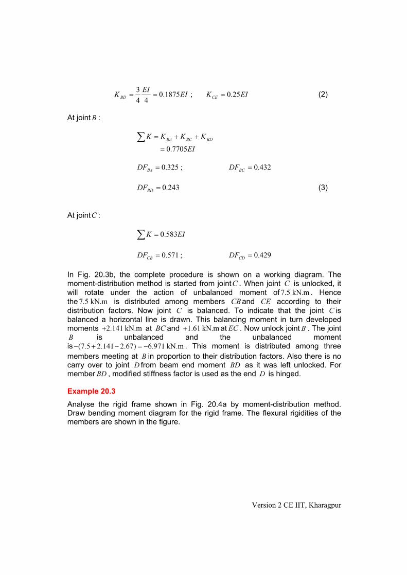
Example 20.3

Analyse the rigid frame shown in Fig. 20.4a by moment-distribution method. Draw bending moment diagram for the rigid frame. The flexural rigidities of the members are shown in the figure.


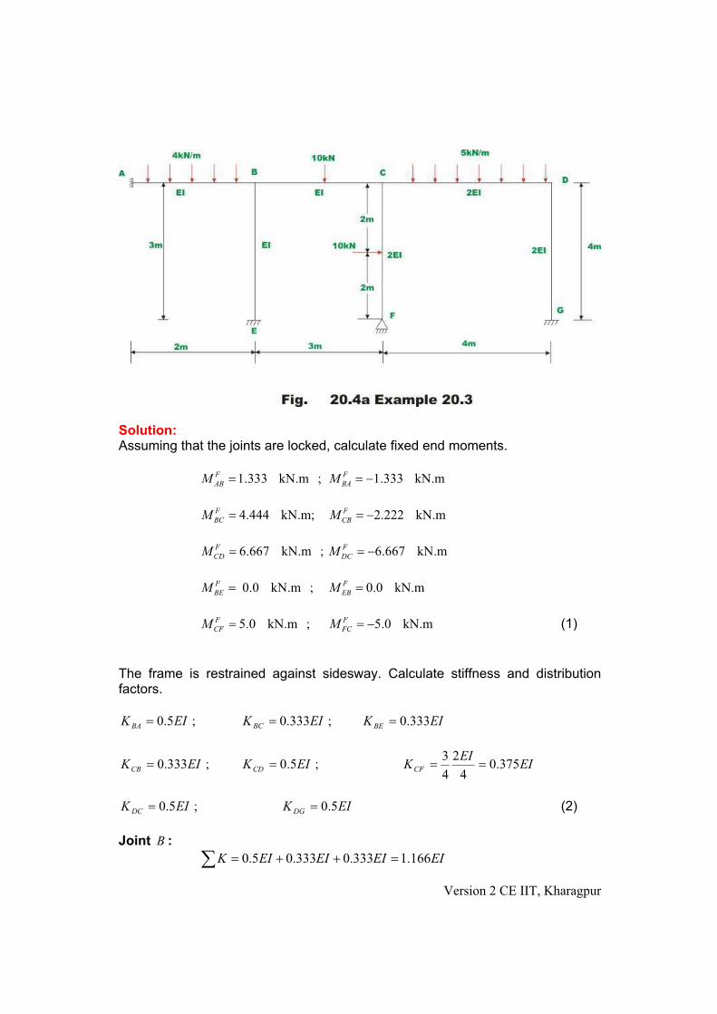
Solution:Assuming that the joints are locked, calculate fixed end moments.

1.333 kN.m ;F

ABM 1.333 kN.mF

BAM !

4.444 kN.m;F

BCM 2.222 kN.mF

CBM !

6.667 kN.m ;F

CDM 6.667 kN.mF

DCM !

0.0 kN.m ;F

BEM 0.0 kN.mF

EBM

5.0 kN.m ;F

CFM (1) 5.0 kN.mF

FCM !

The frame is restrained against sidesway. Calculate stiffness and distribution factors.

EIKEIKEIK BEBCBA 333.0;333.0;5.0

EIEI

KEIKEIK CFCDCB 375.04

2

4

3;5.0;333.0

EIKEIK DGDC 5.0;5.0 (2)

Joint B :

EIEIEIEIK 166.1333.0333.05.0 %% "


286.0;428.0 BCBA DFDF

286.0 BEDF

Joint C :

EIEIEIEIK 208.1375.05.0333.0 %% "

414.0;276.0 CDCB DFDF

31.0 CFDF

Joint :D

EIK 0.1 "

50.0;50.0 DGDC DFDF (3)


The complete moment-distribution method is shown in Fig. 20.4b. The moment-distribution is stopped after three cycles. The moment-distribution is started by releasing and balancing joint . This is repeated for joints C and D B respectively

in that order. After balancing joint , it is left unlocked throughout as it is a hinged joint. After balancing each joint a horizontal line is drawn to indicate that joint has been balanced and locked. When moment-distribution method is finally stopped all joints except fixed joints will be left unlocked.

F

Summary

In this lesson plane frames which are restrained against sidesway are analysed by the moment-distribution method. As many equilibrium equations are written as there are unknown displacements. The reactions of the frames are computed from equations of static equilibrium. The bending moment diagram is drawn for the frame. A few problems are solved to illustrate the procedure. Free-body diagrams are drawn wherever required.



Module 3




Lesson 21


Frames with Sidesway


After reading this chapter the student will be able to

1. Extend moment-distribution method for frames undergoing sidesway. 2. Draw free-body diagrams of plane frame. 3. Analyse plane frames undergoing sidesway by the moment-distribution

method.4. Draw shear force and bending moment diagrams. 5. Sketch deflected shape of the plane frame not restrained against sidesway.

21.1 Introduction

In the previous lesson, rigid frames restrained against sidesway are analyzed using moment-distribution method. It has been pointed in lesson 17, that frames which are unsymmetrical or frames which are loaded unsymmetrically usually get displaced either to the right or to the left. In other words, in such frames apart from evaluating joint rotations, one also needs to evaluate joint translations (sidesway). For example in frame shown in Fig 21.1, the loading is symmetrical but the geometry of frame is unsymmetrical and hence sidesway needs to be considered in the analysis. The number of unknowns is this case are: joint

rotations B and C and member rotation! . Joint B and C get translated by the

same amount as axial deformations are not considered and hence only one independent member rotation need to be considered. The procedure to analyze rigid frames undergoing lateral displacement using moment-distribution method is explained in section 21.2 using an example.


21.2 Procedure

A special procedure is required to analyze frames with sidesway using moment-distribution method. In the first step, identify the number of independent rotations (! ) in the structure. The procedure to calculate independent rotations is

explained in lesson 22. For analyzing frames with sidesway, the method of superposition is used. The structure shown in Fig. 21.2a is expressed as the sum of two systems: Fig. 21.2b and Fig. 21.2c. The systems shown in figures 21.2b and 21.2c are analyzed separately and superposed to obtain the final answer. In system 21.2b, sidesway is prevented by artificial support atC . Apply

all the external loads on frame shown in Fig. 21.2b. Since for the frame, sidesway is prevented, moment-distribution method as discussed in the previous lesson is applied and beam end moments are calculated.

Let and be the balanced moments obtained by

distributing fixed end moments due to applied loads while allowing only joint

rotations (

''''' ,,,, CDCBBCBAAB MMMMM '

DCM

B and C ) and preventing sidesway.

Now, calculate reactions and (ref. Fig 21.3a).they are , 1AH 1DH


22

''

1h

Pa

h

MMH BAABA "

"#

1

''

1h

MMH DCCDD

"# (21.1)

again, (21.2) )( 11 DA HHPR "$#


In Fig 21.2c apply a horizontal force in the opposite direction ofF R . Now

, then the superposition of beam end moments of system (b) and times

(c) gives the results for the original structure. However, there is no way one could

analyze the frame for horizontal force , by moment-distribution method as sway

comes in to picture. Instead of applying , apply arbitrary known displacement /

sidesway ' as shown in the figure. Calculate the fixed end beam moments in

the column

RFk # k

F

F

%

AB and CD for the imposed horizontal displacement. Since joint

displacement is known beforehand, one could use moment-distribution method to

analyse this frame. In this case, member rotations ! are related to joint

translation which is known. Let and are the

balanced moment obtained by distributing the fixed end moments due to

assumed sidesway at joints

'''''''''' ,,,, CDCBBCBAAB MMMMM ''

DCM

'% B and . Now, from statics calculate horizontal

force due to arbitrary sidesway

C

F '% .


2

''''

2h

MMH BAABA

"#

1

''''

2h

MMH DCCDD

"# (21.3)

)( 22 DA HHF "# (21.4)

In Fig 21.2, by method of superposition

RkF # or FRk /#

Substituting the values of R and from equations (21.2) and (21.4), F

)(

)(

22

11

DA

DA

HH

HHPk

"

"$# (21.5)

Now substituting the values of , , and in 21.5, 1AH 2AH 1DH 2DH

&&'

())*

+ ""

""&&

'

())*

+"

"$

#"

12

122

''''''''

''''

h

MM

h

MM

h

MM

h

Pa

h

MMP

kDCCDBAAB

DCCDBAAB

(21.6)

Hence, beam end moment in the original structure is obtained as,

)()( csystembsystemoriginal kMMM "#

If there is more than one independent member rotation, then the above procedure needs to be modified and is discussed in the next lesson.


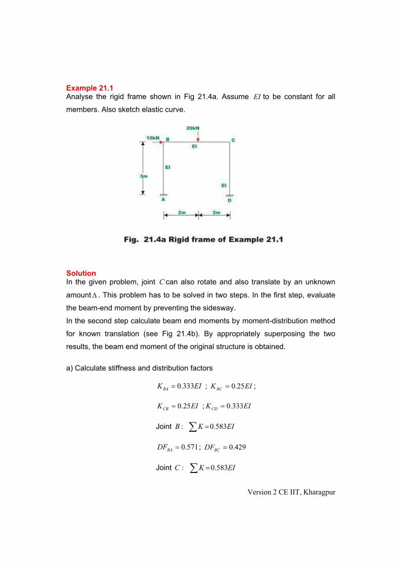
Example 21.1 Analyse the rigid frame shown in Fig 21.4a. Assume EI to be constant for all

members. Also sketch elastic curve.

SolutionIn the given problem, joint can also rotate and also translate by an unknown

amount . This problem has to be solved in two steps. In the first step, evaluate

the beam-end moment by preventing the sidesway.

C

%

In the second step calculate beam end moments by moment-distribution method

for known translation (see Fig 21.4b). By appropriately superposing the two

results, the beam end moment of the original structure is obtained.

a) Calculate stiffness and distribution factors

EIKBA 333.0# ; EIK BC 25.0# ;

EIKCB 25.0# ; EIKCD 333.0#

Joint :B EIK 583.0#,

571.0#BADF ; 429.0#BCDF

Joint :C , # EIK 583.0


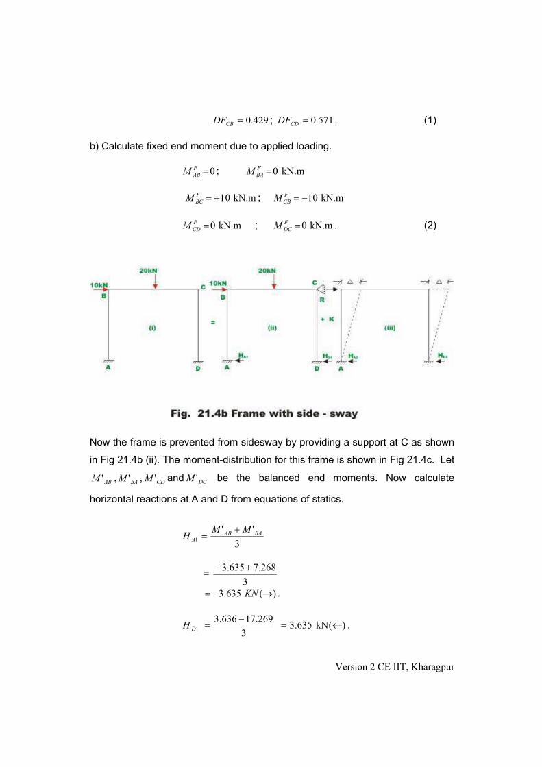
429.0#CBDF ; 571.0#CDDF . (1)

b) Calculate fixed end moment due to applied loading.

0#F

ABM ; kN.m 0#F

BAM

;kN.m01"#F

BCM kN.m01$#F

CBM

kN.m0#F

CDM ; . (2) kN.m0#F

DCM

Now the frame is prevented from sidesway by providing a support at C as shown

in Fig 21.4b (ii). The moment-distribution for this frame is shown in Fig 21.4c. Let

, and be the balanced end moments. Now calculate

horizontal reactions at A and D from equations of statics.

BAAB MM ',' CDM ' DCM '

3

''1

BAABA

MMH

"#

= 3

268.7635.3 !

.)(635.3 "!# KN

)(kN 635.33

269.17636.31 $#

!#DH .


)(kN 10)635.3635.3(10 "!# !!#R (3)

d) Moment-distribution for arbitrary known sidesway '% .

Since is arbitrary, Choose any convenient value. Let '% '% =EI

150 Now calculate

fixed end beam moments for this arbitrary sidesway.

L

EIM F

AB

&6!# )

3

150(

3

6

EI

EI!'!# = kN.m100

kN.m100#F

BAM

kN.m100 ## F

DC

F

CD MM (4)


The moment-distribution for this case is shown in Fig 24.4d. Now calculate

horizontal reactions and .2AH 2DH

=2AH )(kN15.433

48.7698.52$#

2DH = )(kN15.433

49.7697.52$#

)(kN30.86 "!#F


Let be a factor by which the solution of case ( iik i ) needs to be multiplied. Now

actual moments in the frame is obtained by superposing the solution ( ) on the

solution obtained by multiplying case ( ii

ii

i ) by . Thus cancel out the holding

force R such that final result is for the frame without holding force.

k kF

Thus, .RFk #

1161.013.86

10#

!!

#k (5)

Now the actual end moments in the frame are,

ABABAB MkMM ''' #

3.635 0.1161( 76.48) 5.244 kN.mABM # ! #

7.268 0.1161( 52.98) 1.117 kN.mBAM # ! # !

7.268 0.1161( 52.98) 1.117 kN.mBCM # ! #

7.269 0.1161( 52.97) 13.419 kN.mCBM # ! ! # !

7.268 0.1161( 52.97) 13.418 kN.mCDM # #

3.636 0.1161( 76.49) 12.517 kN.mDCM # #

The actual sway is computed as,

EIk

1501161.0' '#%#%

EI

415.17#

The joint rotations can be calculated using slope-deflection equations.

( ABBA

F

ABAB )L

EIMM &** 32

2! # where

LAB

%!#&

( )ABAB

F

BABAL

EIMM &** 32

2! #


In the above equation, except A* and B* all other quantities are known. Solving

for A* and B* ,

EIBA

55.9;0

!## ** .

The elastic curve is shown in Fig. 21.4e.


Example 21.2 Analyse the rigid frame shown in Fig. 21.5a by moment-distribution method. The

moment of inertia of all the members is shown in the figure. Neglect axial

deformations.

Solution:In this frame joint rotations B and and translation of joint C B and need to be

evaluated.

C

a) Calculate stiffness and distribution factors.

EIKEIK BCBA 25.0;333.0 ##

EIKEIK CDCB 333.0;25.0 ##

At jointB :

EIK 583.0#+

429.0;571.0 ## BCBA DFDF

At joint :C

EIK 583.0#+Version 2 CE IIT, Kharagpur

571.0;429.0 ## CDCB DFDF

b) Calculate fixed end moments due to applied loading.

2

2

12 3 39.0 kN.m

6

F

ABM' '

# # ; 9.0 kN.mF

BAM # !

0 kN.mF

BCM # ; 0 kN.mF

CBM #

0 kN.mF

CDM # ; 0 kN.mF

DCM #

c) Prevent sidesway by providing artificial support at C . Carry out moment-

distribution ( Case..ei A in Fig. 21.5b). The moment-distribution for this case is

shown in Fig. 21.5c.


Now calculate horizontal reaction at A and from equations of statics. D

, -1

11.694 3.6146 7.347 kN

6AH

!# # $

, -1

1.154 0.5780.577 kN

3DH

! !# # ! "

, -12 (7.347 0.577) 5.23 kNR # ! ! # ! "

d) Moment-distribution for arbitrary sidesway '% (case B, Fig. 21.5c)

Calculate fixed end moments for the arbitrary sidesway of EI

150'#% .

6 (2 ) 12 150( ) 50 kN.m ; 50 kN.m ;

6 6

F F

AB BA

E I EIM M

L EI&# ! # ' ! # #


6 ( ) 6 150( ) 100 kN.m ; 100 kN.m ;

3 3

F F

CD DC

E I EIM M

L EI&# ! # ! ' ! # #

The moment-distribution for this case is shown in Fig. 21.5d. Using equations of

static equilibrium, calculate reactions and .2AH 2DH

)(395.126

457.41911.322 $#

# kNH A

)(952.393

285.7357.462 $#

# kNH D

)(347.52)952.39395.12( "!# !# kNF

e) Final results

Now, the shear condition for the frame is (vide Fig. 21.5b)


129.0

12)952.39395.12()577.0344.7(

12)()( 2211

#

# !

#

k

k

HHkHH DADA


ABABAB MkMM ''' #

11.694 0.129( 41.457) 17.039 kN.mABM # #

3.614 0.129( 32.911) 0.629 kN.mBAM # ! #

3.614 0.129( 32.911) 0.629 kN.mBCM # ! # !

1.154 0.129( 46.457) 4.853 kN.mCBM # ! ! # !

1.154 0.129( 46.457) 4.853 kN.mCDM # ! #

0.578 0.129( 73.285) 8.876 kN.mDCM # ! #

The actual sway

EIk

150129.0' '#%#%

EI

35.19#

The joint rotations can be calculated using slope-deflection equations.

( )&** 32)2(2

! #! BA

F

ABABL

IEMM

or

( ) ./

012

345

678

9 !!#./

012

3 !# L

EIMM

EI

L

L

EIMM

EI

L F

ABAB

F

ABABBA

&&**

12

4

12

42

( ) ./

012

345

678

9 !!#./

012

3 !# L

EIMM

EI

L

L

EIMM

EI

L F

BABA

F

BABAAB

&&**

12

4

12

42

17.039 kN.mABM #


0.629 kN.mBAM #

, - 9 0.129(50) 15.45 kN.mF

ABM # #

, - 9 0.129(50) 2.55 kN.mF

BAM # ! # !

1change in near end + - change in far end

2

3

1(17.039 15.45) (0.629 2.55)

20.0

36

A EIL

EI

*

9 67 48 5#

9 6! ! 7 48 5# #

4.769B

EI* #

Example 21.3 Analyse the rigid frame shown in Fig. 21.6a. The moment of inertia of all the

members are shown in the figure.


Solution:a) Calculate stiffness and distribution factors

EIKEIEI

K BCBA 50.0;392.01.5

2###

EIKEIK CDCB 392.0;50.0 ##

At jointB :

EIK 892.0#+

561.0;439.0 ## BCBA DFDF

At joint :C

EIK 892.0#+

439.0;561.0 ## CDCB DFDF (1)

b) Calculate fixed end moments due to applied loading.

0 kN.mF F F F

AB BA CD DCM M M M# # # #

2.50 kN.mF

BCM #

2.50 kN.mF

CBM # ! (2)

c) Prevent sidesway by providing artificial support atC . Carry out moment-

distribution for this case as shown in Fig. 21.6b.


Now calculate reactions from free body diagram shown in Fig. 21.5d.


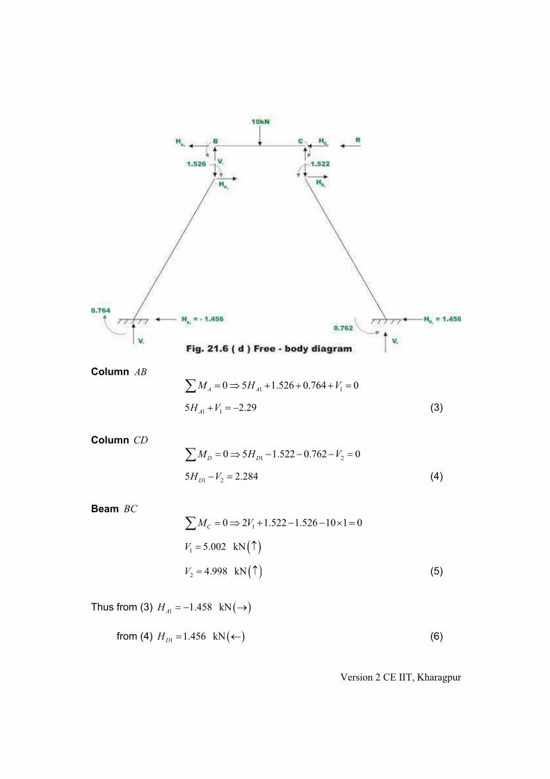
Column AB

1 10 5 1.526 0.764 0A AM H V# : #+

1 15 2.29AH V # ! (3)

Column CD

10 5 1.522 0.762 0D DM H V# : ! ! ! #+ 2

(4) 1 25 2.284DH V! #

Beam BC

10 2 1.522 1.526 10 1 0CM V# : ! ! ' #+

, -1 5.002 kNV # ;

, -2 4.998 kNV # ; (5)

Thus from (3) , -1 1.458 kNAH # ! "

from (4) , -1 1.456 kNDH # $ (6)



0#

, -1 10 5

5.002 kN

X A DF H H R

R

# !

# $

+ (7)

d) Moment-distribution for arbitrary sidesway '% .

Calculate fixed end beam moments for arbitrary sidesway of

EI

75.12'#%

The member rotations for this arbitrary sidesway is shown in Fig. 21.6e.

11

" ';

cos 5AB

AB AB

BB

L L

5.1 '&

<% % %

# # ! % # #

2

2 '0.4 '

5

%% # # %

'( )

5AB clockwise&

%# ! ;

'( )

5CD clockwise&

%# !

2 2 ' tan '( )

2 2 5BC counterclockwise

<&

% % %# # #

6 6 (2 ) 12.756.0 kN.m

5.1 5

F ABAB AB

AB

EI E IM

L EI& 9 6# ! # ! ! # 7 4

8 5

6.0 kN.mF

BAM #

6 6 ( ) 12.757.65 kN.m

2 5

F BCBC BC

BC

EI E IM

L EI& 9 6# ! # ! # !7 4

8 5

7.65 kN.mF

CBM # !

6 6 (2 ) 12.756.0 kN.m

5.1 5

F CDCD CD

CD

EI E IM

L EI& 9 6# ! # ! ! # 7 4

8 5

6.0 kN.mF

DCM #

The moment-distribution for the arbitrary sway is shown in Fig. 21.6f. Now

reactions can be calculated from statics.


Column AB

2 10 5 6.283 6.567 0A AM H V# : ! ! #+

1 15 12.85AH V # (3)

Column CD

2 20 5 6.567 6.283 0D DM H V# : ! ! ! #+

1 25 12.85DH V! # (4)

Beam BC

10 2 6.567 6.567 0CM V# : #+

, -1 6.567V kN , -2 6.567 kNV# ! = ; ; (5) #

Thus from 3 , -2 3.883 kNAH # $

from 4 (6) , -2 3.883 kNDH # $


, -7.766 kNF # $ (7)

e) Final results

RFk #

644.0766.7

002.5##k


ABABAB MkMM ''' #

0.764 0.644( 6.283) 3.282 kN.mABM # ! #

1.526 0.644( 6.567) 2.703 kN.mBAM # ! #

1.526 0.644( 6.567) 2.703 kN.mBCM # ! # !

1.522 0.644( 6.567) 5.751 kN.mCBM # ! ! # ! !

1.522 0.644(6.567) 5.751 kN.mCDM # #

0.762 0.644(6.283) 4.808 kN.mDCM # #

The actual sway

EIk

75.12644.0' '#%#%

EI

212.8#

Summary

In this lesson, the frames which are not restrained against sidesway are identified and solved by the moment-distribution method. The moment-distribution method is applied in two steps: in the first step, the frame prevented from sidesway but subjected to external loads is analysed and subsequently, the frame which is undergoing an arbitrary but known sidesway is analysed. Using shear equation for the frame, the moments in the frame is obtained. The numerical examples are explained with the help of free-body diagrams. The deflected shape of the frame is sketched to understand its deformation under external loads.


Module 3




Lesson 22

The Multistory Frames with Sidesway



After reading this chapter the student will be able to 1. Identify the number of independent rotational degrees of freedom of a rigid

frame.2. Write appropriate number of equilibrium equations to solve rigid frame

having more than one rotational degree of freedom. 3. Draw free-body diagram of multistory frames. 4. Analyse multistory frames with sidesway by the slope-deflection method. 5. Analyse multistory frames with sidesway by the moment-distribution

method.

22.1 Introduction

In lessons 17 and 21, rigid frames having single independent member rotational

( !

"#$

% &'h

( ) degree of freedom (or joint translation& ) is solved using slope-

deflection and moment-distribution method respectively. However multistory frames usually have more than one independent rotational degree of freedom. Such frames can also be analysed by slope-deflection and moment-distribution methods. Usually number of independent member rotations can be evaluated by inspection. However if the structure is complex the following method may be adopted. Consider the structure shown in Fig. 22.1a. Temporarily replace all rigid joints of the frame by pinned joint and fixed supports by hinged supports as shown in Fig. 22.1b. Now inspect the stability of the modified structure. If one or more joints are free to translate without any resistance then the structure is geometrically unstable. Now introduce forces in appropriate directions to the structure so as to make it stable. The number of such externally applied forces represents the number of independent member rotations in the structure.


In the modified structure Fig. 22.1b, two forces are required to be applied at level and level CD BF for stability of the structure. Hence there are two independent

member rotations ) *( that need to be considered apart from joint rotations in the

analysis.

The number of independent rotations to be considered for the frame shown in Fig. 22.2a is three and is clear from the modified structure shown in Fig. 22.2b.

From the above procedure it is clear that the frame shown in Fig. 22.3a has three independent member rotations and frame shown in Fig 22.4a has two independent member rotations.


For the gable frame shown in Fig. 22.4a, the possible displacements at each joint are also shown. Horizontal displacement is denoted by and vertical

displacement is denoted by v . Recall that in the analysis, we are not considering

u


the axial deformation. Hence at B and only horizontal deformation is possible and joint C can have both horizontal and vertical deformation. The

displacements and should be such that the lengths and

must not change as the axial deformation is not considered. Hence we can have only two independent translations. In the next section slope-deflection method as applied to multistoried frame is discussed.

D

DCB uuu ,, Du BC CD

22.2 Slope-deflection method

For the two story frame shown in Fig. 22.5, there are four joint rotations

) EDCB *and+++ ,,+ and two independent joint translations (sidesway) at the

level of CDand at the level of

1&

2& BE .

Six simultaneous equations are required to evaluate the six unknowns (four rotations and two translations). For each of the member one could write two slope-deflection equations relating beam end moments to externally applied

loads and displacements (rotations and translations). Four of the required six

equations are obtained by considering the moment equilibrium of joint and

)(i

)(ii

DCB ,,

E respectively. For example,


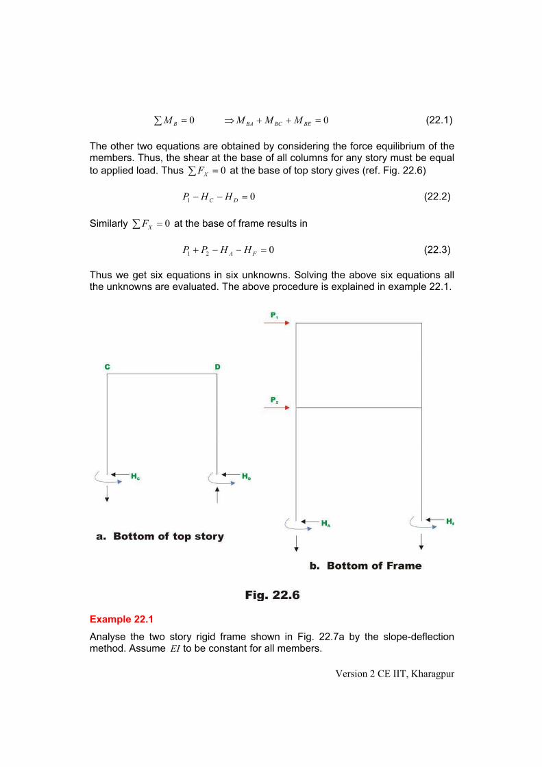
, '--.' 00 BEBCBAB MMMM (22.1)

The other two equations are obtained by considering the force equilibrium of the members. Thus, the shear at the base of all columns for any story must be equal

to applied load. Thus at the base of top story gives (ref. Fig. 22.6) , ' 0XF

01 '// DC HHP (22.2)

Similarly at the base of frame results in, ' 0XF

021 '//- FA HHPP (22.3)

Thus we get six equations in six unknowns. Solving the above six equations all the unknowns are evaluated. The above procedure is explained in example 22.1.

Example 22.1

Analyse the two story rigid frame shown in Fig. 22.7a by the slope-deflection method. Assume EI to be constant for all members.


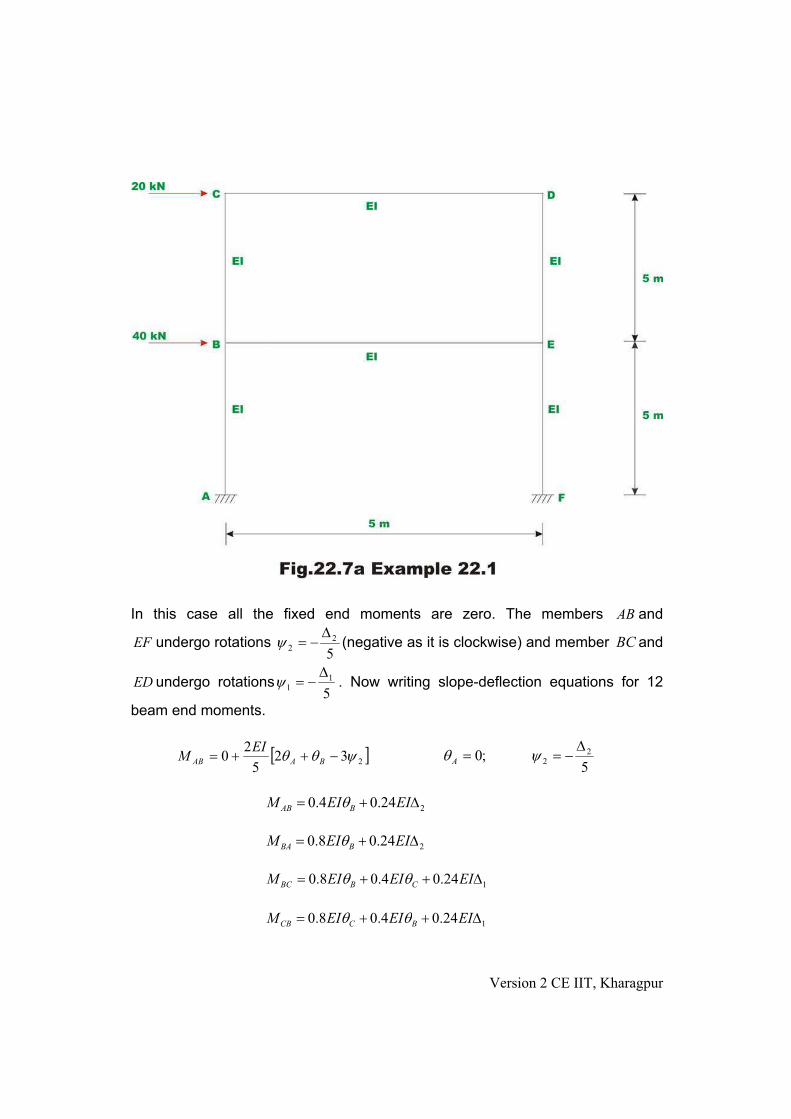
In this case all the fixed end moments are zero. The members AB and

EF undergo rotations 5

22

&/'( (negative as it is clockwise) and member andBC

ED undergo rotations5

11

&/'( . Now writing slope-deflection equations for 12

beam end moments.

0 12325

20 (++ /--' BAAB

EIM ;0'A+

5

22

&/'(

224.04.0 &-' EIEIM BAB +

224.08.0 &-' EIEIM BBA +

124.04.08.0 &--' EIEIEIM CBBC ++

124.04.08.0 &--' EIEIEIM BCCB ++


EBBE EIEIM ++ 4.08.0 -'

BEEB EIEIM ++ 4.08.0 -'

DCCD EIEIM ++ 4.08.0 -'

CDDC EIEIM ++ 4.08.0 -'

124.04.08.0 &--' EIEIEIM EDDE ++

124.04.08.0 &--' EIEIEIM DEED ++

224.08.0 &-' EIEIM EEF +

224.04.0 &-' EIEIM EFE + (1)


Moment equilibrium of joint andDCB ,, E requires that (vide Fig. 22.7c).

0'-- BEBCBA MMM

0'- CDCB MM

0'- DEDC MM

0'-- EFEDEB MMM (2)

The required two more equations are written considering the horizontal

equilibrium at each story level. , ' 0.. XFei (vide., Fig. 22.7d). Thus,

20'- DC HH

60'- FA HH (3)

Considering the equilibrium of column andBCEFAB ,, ED , we get (vide 22.7c)


5

CBBCC

MMH

-'

5

EDDED

MMH

-'

5

BAABA

MMH

-'

5

FEEFF

MMH

-' (4)

Using equation (4), equation (3) may be written as,

100'--- EDDECBBC MMMM

300'--- FEEFBAAB MMMM (5)

Substituting the beam end moments from equation (1) in (2) and (5) the required equations are obtained. Thus,

024.024.04.04.04.2 21 '&-&--- ECB +++

024.04.04.06.1 1 '&--- BDC +++

024.04.04.06.1 1 '&--- ECD +++

024.024.04.04.04.2 21 '&-&--- DBE +++

10096.02.12.12.12.1 1 '&---- EDCB ++++

30096.02.12.1 2 '&--- EB ++ (6)

Solving above equations, yields

EIEI

EIEIEIEIDECB

27.477;

12.337

;909.65

;273.27

;273.27

;909.65

21 '&'&

/'

/'

/'

/' ++++

(7)


Substituting the above values of rotations and translations in equation (1) beam end moments are evaluated. They are,

88.18 kN.m ; 61.81 kN.mAB BAM M' '

17.27 kN.m ; 32.72. kN.mBC CBM M' '

79.09 kN.m ; 79.09 kN.mBE EBM M' / ' /

32.72 kN.m ; 32.72 kN.mCD DCM M' / ' /

32.72 kN.m ; 17.27 kN.mDE EDM M' '

61.81 kN.m ; 88.18 kN.mEF FEM M' '

22.3 Moment-distribution method

The two-story frame shown in Fig. 22.8a has two independent sidesways or member rotations. Invoking the method of superposition, the structure shown in Fig. 22.8a is expressed as the sum of three systems;

1) The system shown in Fig. 22.8b, where in the sidesway is completely prevented by introducing two supports at E and . All external loads are applied on this frame.

D

2) System shown in Fig. 22.8c, wherein the support E is locked against sidesway and joint and are allowed to displace horizontally. Apply

arbitrary sidesway and calculate fixed end moments in column and

C D

1'& BC

DE . Using moment-distribution method, calculate beam end moments. 3) Structure shown in Fig. 22.8d, the support is locked against sidesway

and joints D

B and E are allowed to displace horizontally by removing the support at E . Calculate fixed end moments in column AB and EF for an

arbitrary sidesway as shown the in figure. Since joint displacement as

known beforehand, one could use the moment-distribution method to analyse the frame.

2'&


All three systems are analysed separately and superposed to obtain the final answer. Since structures 22.8c and 22.8d are analysed for arbitrary sidesway

and respectively, the end moments and the displacements of these two

analyses are to be multiplied by constants and before superposing with the

results obtained in Fig. 22.8b. The constants and must be such that

1'& 2'&

1k 2k

1k 2k


111 ' &'&k and 222 ' &'&k . (22.4)

The constants and are evaluated by solving shear equations. From Fig.

22.9, it is clear that the horizontal forces developed at the beam level in Fig.

22.9c and 22.9d must be equal and opposite to the restraining force applied at the restraining support at in Fig. 22.9b. Thus,

1k 2k

CD

D

) * ) * 1332221 PHHkHHk DCDC '--- (23.5)

From similar reasoning, from Fig. 22.10, one could write,

) * ) * 2332221 PHHkHHk FAFA '--- (23.6)

Solving the above two equations, and are calculated. 1k 2k


Example 22.2

Analyse the rigid frame of example 22.1 by the moment-distribution method.

Solution:First calculate stiffness and distribution factors for all the six members.

EIKEIKEIK

EIKEIK

EIKEIK

EIKEIKEIK

EFEDEB

DEDC

CDCB

BEBCBA

20.0;20.0;20.0

;20.0;20.0

;20.0;20.0

;20.0;20.0;20.0

'''

''

''

'''

(1)

Joint :B , ' EIK 60.0

333.0;333.0;333.0 ''' BEBCBA DFDFDF


JointC : , ' EIK 40.0

50.0;50.0 '' CDCB DFDF

Joint :D , ' EIK 40.0

50.0;50.0 '' DEDC DFDF

Joint E : , ' EIK 60.0

333.0;333.0;333.0 ''' EFEDEB DFDFDF (2)

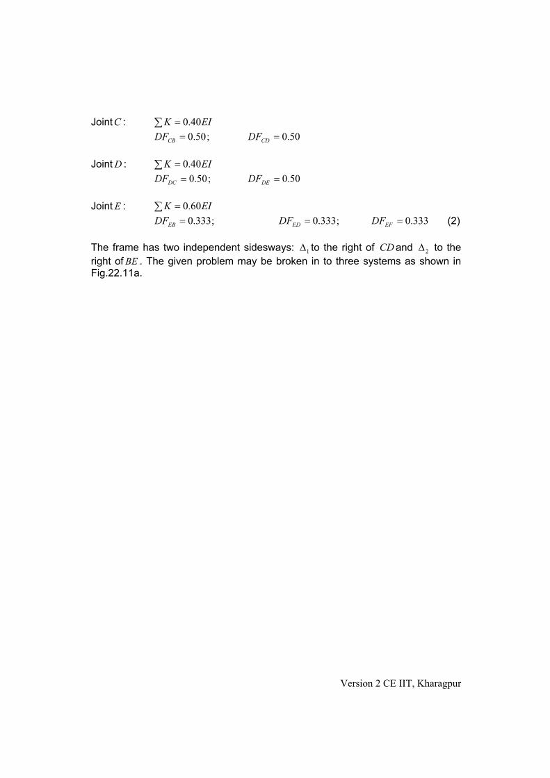
The frame has two independent sidesways: 1& to the right of CDand to the

right of2&

BE . The given problem may be broken in to three systems as shown in Fig.22.11a.


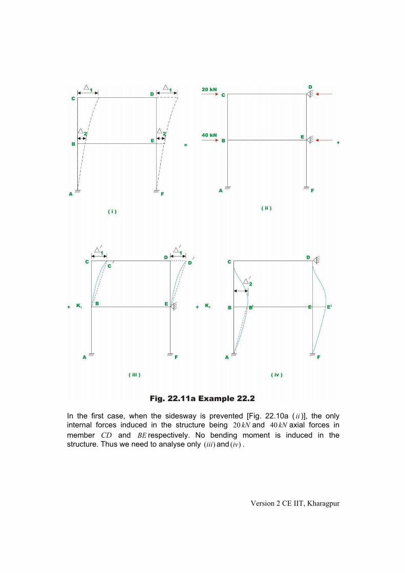
In the first case, when the sidesway is prevented [Fig. 22.10a ( )], the only

internal forces induced in the structure being and axial forces in

member and

ii

kN20 kN40

CD BE respectively. No bending moment is induced in the

structure. Thus we need to analyse only and .)(iii )(iv


Case I :

Moment-distribution for sidesway 1'& at beam CD [Fig. 22.1qa ( )]. Let the

arbitrary sidesway be

iii

EI

25'1 '& . Thus the fixed end moment in column CBand

DE due to this arbitrary sidesway is

1

2

6 ' 6 256.0 kN.m

25

F F

BC CB

EI EIM M

L EI

&' ' ' 2 ' -

6.0 kN.mF F

ED DEM M' ' - (3)

Now moment-distribution is carried out to obtain the balanced end moments. The whole procedure is shown in Fig. 22.11b. Successively joint andBCD ,, E are

released and balanced.


From the free body diagram of the column shown in Fig. 22.11c, the horizontal forces are calculated. Thus,


2

3.53 3.171.34 kN;

5CH

-' ' 2 1.34 kNDH '

2

0.70 1.410.42 kN;

5AH

/ /' ' / 2 0.42 kNFH ' / (4)

Case II :

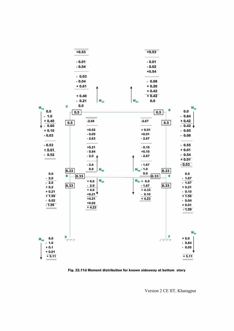
Moment-distribution for sidesway 2'& at beam BE [Fig. 22.11a ( iv )]. Let the

arbitrary sidesway be EI

25'2 '&

Thus the fixed end moment in column AB and EF due to this arbitrary sidesway is

2

2

6 ' 6 256.0 kN.m

25

F F

AB BA

EI EIM M

L EI

&' ' ' 2 ' -

6.0 kN.mF F

FE EFM M' ' - (5)

Moment-distribution is carried out to obtain the balanced end moments as shown in Fig. 22.11d. The whole procedure is shown in Fig. 22.10b. Successively joint

andBCD ,, E are released and balanced.


From the free body diagram of the column shown in Fig. 22.11e, the horizontal forces are calculated. Thus,

3 3

1.59 0.530.42 kN; 0.42 kN

5C DH H

/ /' ' / ' /

3 3

5.11 4.231.86 kN; 1.86 kN

5A FH H

-' ' ' (6)

For evaluating constants and , we could write, (see Fig. 22.11a, 22.11c and

22.11d).1k 2k

) * ) * 20332221 '--- DCDC HHkHHk

) * ) * 60332221 '--- FAFA HHkHHk

) * ) * 2042.042.034.134.1 21 '//-- kk

) * ) * 6086.186.142.042.0 21 '--// kk


) * ) * 1042.034.1 21 '/- kk

) * ) * 3086.142.0 21 '-/ kk

Solving which, 17.1947.13 21 '' kk (7)

Thus the final moments are,

88.52 kN.m ; 62.09 kN.mAB BAM M' '

17.06 kN.m ; 32.54. kN.mBC CBM M' '

79.54 kN.m ; 79.54 kN.mBE EBM M' / ' /

32.54 kN.m ; 32.54 kN.mCD DCM M' / ' /

32.54 kN.m ; 17.06 kN.mDE EDM M' '

62.09 kN.m ; 88.52 kN.mEF FEM M' ' (8)

Summary

A procedure to identify the number of independent rotational degrees of freedom of a rigid frame is given. The slope-deflection method and the moment-distribution method are extended in this lesson to solve rigid multistory frames having more than one independent rotational degrees of freedom. A multistory frames having side sway is analysed by the slope-deflection method and the moment-distribution method. Appropriate number of equilibrium equations is written to evaluate all unknowns. Numerical examples are explained with the help of free-body diagrams.


Module 4


Structures by the Direct StiffnessMethod


Lesson 23

The Direct Stiffness Method: An

Introduction


Instructional Objectives:

After reading this chapter the student will be able to 1. Differentiate between the direct stiffness method and the displacement

method.2. Formulate flexibility matrix of member. 3. Define stiffness matrix. 4. Construct stiffness matrix of a member. 5. Analyse simple structures by the direct stiffness matrix.

23.1 Introduction

All known methods of structural analysis are classified into two distinct groups:-

(i) force method of analysis and (ii) displacement method of analysis.

In module 2, the force method of analysis or the method of consistent deformation is discussed. An introduction to the displacement method of analysis is given in module 3, where in slope-deflection method and moment- distribution method are discussed. In this module the direct stiffness method is discussed. In the displacement method of analysis the equilibrium equations are written by expressing the unknown joint displacements in terms of loads by using load-displacement relations. The unknown joint displacements (the degrees of freedom of the structure) are calculated by solving equilibrium equations. The slope-deflection and moment-distribution methods were extensively used before the high speed computing era. After the revolution in computer industry, only direct stiffness method is used.

The displacement method follows essentially the same steps for both statically determinate and indeterminate structures. In displacement /stiffness method of analysis, once the structural model is defined, the unknowns (joint rotations and translations) are automatically chosen unlike the force method of analysis. Hence, displacement method of analysis is preferred to computer implementation. The method follows a rather a set procedure. The direct stiffness method is closely related to slope-deflection equations.

The general method of analyzing indeterminate structures by displacement method may be traced to Navier (1785-1836). For example consider a four member truss as shown in Fig.23.1.The given truss is statically indeterminate to second degree as there are four bar forces but we have only two equations of equilibrium. Denote each member by a number, for example (1), (2), (3) and (4).

Let i be the angle, the i-th member makes with the horizontal. Under the


Example 17 - دچينې ويب ... · Example 17.3 Analyse the rigid ... In this lesson, ... Module...

Documents

Transcript of Example 17 - دچينې ويب ... · Example 17.3 Analyse the rigid ... In this lesson, ... Module...