Exam 3 ReviewExam 3 Review Optimization Suppose that a business is transitioning from using...
82
Exam 3 Review Exam 3 Review
Transcript of Exam 3 ReviewExam 3 Review Optimization Suppose that a business is transitioning from using...

Exam 3 Review
Exam 3 Review

Notions from Exam 2
I Cost C (x) (usually given)
I Average cost C (x)
C (x) =C (x)
x,
I Marginal Avergage Cost
d
dxC (x) =
d
dx
(C (x)
x
)
Exam 3 Review

Notions from Exam 2
I Cost C (x) (usually given)
I Average cost C (x)
C (x) =C (x)
x,
I Marginal Avergage Cost
d
dxC (x) =
d
dx
(C (x)
x
)
Exam 3 Review

Notions from Exam 2
I Cost C (x) (usually given)
I Average cost C (x)
C (x) =C (x)
x,
I Marginal Avergage Cost
d
dxC (x) =
d
dx
(C (x)
x
)
Exam 3 Review

Notions from Exam 2
I Cost C (x) (usually given)
I Average cost C (x)
C (x) =C (x)
x,
I Marginal Avergage Cost
d
dxC (x) =
d
dx
(C (x)
x
)
Exam 3 Review

Notions from Exam 2
I Cost C (x) (usually given)
I Average cost C (x)
C (x) =C (x)
x,
I Marginal Avergage Cost
d
dxC (x) =
d
dx
(C (x)
x
)
Exam 3 Review

Notions from Exam 2
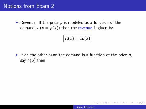
I Revenue: If the price p is modeled as a function of thedemand x (p = p(x)) then the revenue is given by
R(x) = xp(x)
I If on the other hand the demand is a function of the price p,say f (p) then
R(p) = pf (p)
I Marginal revenue: derivative of the revenue R as a functioneither of p or of x .
Exam 3 Review

Notions from Exam 2
I Revenue: If the price p is modeled as a function of thedemand x (p = p(x)) then the revenue is given by
R(x) = xp(x)
I If on the other hand the demand is a function of the price p,say f (p) then
R(p) = pf (p)
I Marginal revenue: derivative of the revenue R as a functioneither of p or of x .
Exam 3 Review

Notions from Exam 2
I Profit
P(x) = R(x)− C (x)
I Marginal Profit
P′(x) = R
′(x)− C
′(x)
Exam 3 Review

Notions from Exam 2
I Profit
P(x) = R(x)− C (x)
I Marginal Profit
P′(x) = R
′(x)− C
′(x)
Exam 3 Review

Notions from Exam 2
I Profit
P(x) = R(x)− C (x)
I Marginal Profit
P′(x) = R
′(x)− C
′(x)
Exam 3 Review

Notions from Exam 2
I Profit
P(x) = R(x)− C (x)
I Marginal Profit
P′(x) = R
′(x)− C
′(x)
Exam 3 Review

Notions from Exam 2
I Profit
P(x) = R(x)− C (x)
I Marginal Profit
P′(x) = R
′(x)− C
′(x)
Exam 3 Review
Marginal Functions in Economics
I Elasticity of demand
I p price
I x demand (as a function of the price)
I If x = x(p) = f (p) then the elasticity of demand is defined as
E (p) = −pf ′(p)
f (p)
or
E (p) = −px ′(p)
x(p)
Exam 3 Review

Marginal Functions in Economics
I Elasticity of demand
I p price
I x demand (as a function of the price)
I If x = x(p) = f (p) then the elasticity of demand is defined as
E (p) = −pf ′(p)
f (p)
or
E (p) = −px ′(p)
x(p)
Exam 3 Review

Marginal Functions in Economics
I Elasticity of demand
I p price
I x demand (as a function of the price)
I If x = x(p) = f (p) then the elasticity of demand is defined as
E (p) = −pf ′(p)
f (p)
or
E (p) = −px ′(p)
x(p)
Exam 3 Review

Marginal Functions in Economics
I Elasticity of demand
I p price
I x demand (as a function of the price)
I If x = x(p) = f (p) then the elasticity of demand is defined as
E (p) = −pf ′(p)
f (p)
or
E (p) = −px ′(p)
x(p)
Exam 3 Review

Marginal Functions in Economics
I Elasticity of demand
I p price
I x demand (as a function of the price)
I If x = x(p) = f (p) then the elasticity of demand is defined as
E (p) = −pf ′(p)
f (p)
or
E (p) = −px ′(p)
x(p)
Exam 3 Review

Marginal Functions in Economics
I Elasticity of demand
I p price
I x demand (as a function of the price)
I If x = x(p) = f (p) then the elasticity of demand is defined as
E (p) = −pf ′(p)
f (p)
or
E (p) = −px ′(p)
x(p)
Exam 3 Review

Marginal Functions in Economics
I Elasticity of demand
I p price
I x demand (as a function of the price)
I If x = x(p) = f (p) then the elasticity of demand is defined as
E (p) = −pf ′(p)
f (p)
or
E (p) = −px ′(p)
x(p)
Exam 3 Review

Optimization
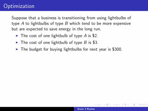
Suppose that a business is transitioning from using lightbulbs oftype A to lightbulbs of type B which tend to be more expensivebut are expected to save energy in the long run.
I The cost of one lightbulb of type A is $2.
I The cost of one lightbulb of type B is $3.
I The budget for buying lightbulbs for next year is $300.
I The expected cost of using x lightbulbs of type A and ylightbulbs of type B is
c(x , y) = 8x2 + 9y2 + 10x + 15y .
I Find the number of lightbulbs of type A needed to minimizethe expected cost c(x , y) if one assumes that the entirebudget for buying lightbulbs has to be exhausted.
Exam 3 Review

Optimization
Suppose that a business is transitioning from using lightbulbs oftype A to lightbulbs of type B which tend to be more expensivebut are expected to save energy in the long run.
I The cost of one lightbulb of type A is $2.
I The cost of one lightbulb of type B is $3.
I The budget for buying lightbulbs for next year is $300.
I The expected cost of using x lightbulbs of type A and ylightbulbs of type B is
c(x , y) = 8x2 + 9y2 + 10x + 15y .
I Find the number of lightbulbs of type A needed to minimizethe expected cost c(x , y) if one assumes that the entirebudget for buying lightbulbs has to be exhausted.
Exam 3 Review

Optimization
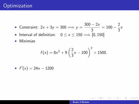
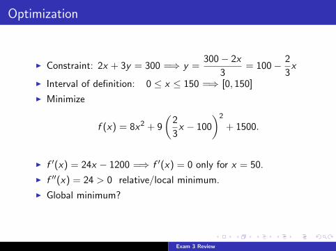
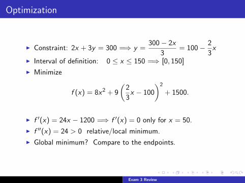
I Constraint: 2x + 3y = 300 =⇒ y =300− 2x
3= 100− 2
3x
I Interval of definition: 0 ≤ x ≤ 150 =⇒ [0, 150]
I Minimize
f (x) = 8x2 + 9
(2
3x − 100
)2
+ 1500.
I f ′(x) = 24x − 1200 =⇒ f ′(x) = 0 only for x = 50.
I f ′′(x) = 24 > 0 relative/local minimum.
I Global minimum? Compare to the endpoints.
Exam 3 Review

Optimization
I Constraint: 2x + 3y = 300 =⇒ y =300− 2x
3= 100− 2
3x
I Interval of definition:
0 ≤ x ≤ 150 =⇒ [0, 150]
I Minimize
f (x) = 8x2 + 9
(2
3x − 100
)2
+ 1500.
I f ′(x) = 24x − 1200 =⇒ f ′(x) = 0 only for x = 50.
I f ′′(x) = 24 > 0 relative/local minimum.
I Global minimum? Compare to the endpoints.
Exam 3 Review

Optimization
I Constraint: 2x + 3y = 300 =⇒ y =300− 2x
3= 100− 2
3x
I Interval of definition: 0 ≤ x ≤ 150 =⇒ [0, 150]
I Minimize
f (x) = 8x2 + 9
(2
3x − 100
)2
+ 1500.
I f ′(x) = 24x − 1200 =⇒ f ′(x) = 0 only for x = 50.
I f ′′(x) = 24 > 0 relative/local minimum.
I Global minimum? Compare to the endpoints.
Exam 3 Review

Optimization
I Constraint: 2x + 3y = 300 =⇒ y =300− 2x
3= 100− 2
3x
I Interval of definition: 0 ≤ x ≤ 150 =⇒ [0, 150]
I Minimize
f (x) = 8x2 + 9
(2
3x − 100
)2
+ 1500.
I f ′(x) = 24x − 1200 =⇒ f ′(x) = 0 only for x = 50.
I f ′′(x) = 24 > 0 relative/local minimum.
I Global minimum? Compare to the endpoints.
Exam 3 Review
Optimization
I Constraint: 2x + 3y = 300 =⇒ y =300− 2x
3= 100− 2
3x
I Interval of definition: 0 ≤ x ≤ 150 =⇒ [0, 150]
I Minimize
f (x) = 8x2 + 9
(2
3x − 100
)2
+ 1500.
I f ′(x) = 24x − 1200
=⇒ f ′(x) = 0 only for x = 50.
I f ′′(x) = 24 > 0 relative/local minimum.
I Global minimum? Compare to the endpoints.
Exam 3 Review

Optimization
I Constraint: 2x + 3y = 300 =⇒ y =300− 2x
3= 100− 2
3x
I Interval of definition: 0 ≤ x ≤ 150 =⇒ [0, 150]
I Minimize
f (x) = 8x2 + 9
(2
3x − 100
)2
+ 1500.
I f ′(x) = 24x − 1200 =⇒ f ′(x) = 0 only for x = 50.
I f ′′(x) = 24 > 0 relative/local minimum.
I Global minimum? Compare to the endpoints.
Exam 3 Review

Optimization
I Constraint: 2x + 3y = 300 =⇒ y =300− 2x
3= 100− 2
3x
I Interval of definition: 0 ≤ x ≤ 150 =⇒ [0, 150]
I Minimize
f (x) = 8x2 + 9
(2
3x − 100
)2
+ 1500.
I f ′(x) = 24x − 1200 =⇒ f ′(x) = 0 only for x = 50.
I f ′′(x) = 24 > 0
relative/local minimum.
I Global minimum? Compare to the endpoints.
Exam 3 Review

Optimization
I Constraint: 2x + 3y = 300 =⇒ y =300− 2x
3= 100− 2
3x
I Interval of definition: 0 ≤ x ≤ 150 =⇒ [0, 150]
I Minimize
f (x) = 8x2 + 9
(2
3x − 100
)2
+ 1500.
I f ′(x) = 24x − 1200 =⇒ f ′(x) = 0 only for x = 50.
I f ′′(x) = 24 > 0 relative/local minimum.
I Global minimum? Compare to the endpoints.
Exam 3 Review
Optimization
I Constraint: 2x + 3y = 300 =⇒ y =300− 2x
3= 100− 2
3x
I Interval of definition: 0 ≤ x ≤ 150 =⇒ [0, 150]
I Minimize
f (x) = 8x2 + 9
(2
3x − 100
)2
+ 1500.
I f ′(x) = 24x − 1200 =⇒ f ′(x) = 0 only for x = 50.
I f ′′(x) = 24 > 0 relative/local minimum.
I Global minimum?
Compare to the endpoints.
Exam 3 Review
Optimization
I Constraint: 2x + 3y = 300 =⇒ y =300− 2x
3= 100− 2
3x
I Interval of definition: 0 ≤ x ≤ 150 =⇒ [0, 150]
I Minimize
f (x) = 8x2 + 9
(2
3x − 100
)2
+ 1500.
I f ′(x) = 24x − 1200 =⇒ f ′(x) = 0 only for x = 50.
I f ′′(x) = 24 > 0 relative/local minimum.
I Global minimum? Compare to the endpoints.
Exam 3 Review

Optimization
I Look at f ′(0) = −1200 < 0 and atf ′(150) = 3600− 1200 = 2400 > 0
I The endpoints cannot be minimizers
I Evaluate f (0), f (50) and f (150) directly.
Exam 3 Review

Optimization
I Look at f ′(0) = −1200 < 0 and atf ′(150) = 3600− 1200 = 2400 > 0
I The endpoints cannot be minimizers
I Evaluate f (0), f (50) and f (150) directly.
Exam 3 Review

Optimization
I Look at f ′(0) = −1200 < 0
and atf ′(150) = 3600− 1200 = 2400 > 0
I The endpoints cannot be minimizers
I Evaluate f (0), f (50) and f (150) directly.
Exam 3 Review

Optimization
I Look at f ′(0) = −1200 < 0 and atf ′(150) = 3600− 1200 = 2400 > 0
I The endpoints cannot be minimizers
I Evaluate f (0), f (50) and f (150) directly.
Exam 3 Review

Optimization
I Look at f ′(0) = −1200 < 0 and atf ′(150) = 3600− 1200 = 2400 > 0
I The endpoints cannot be minimizers
I Evaluate f (0), f (50) and f (150) directly.
Exam 3 Review

Optimization
I Look at f ′(0) = −1200 < 0 and atf ′(150) = 3600− 1200 = 2400 > 0
I The endpoints cannot be minimizers
I Evaluate f (0), f (50) and f (150) directly.
Exam 3 Review

Optimization
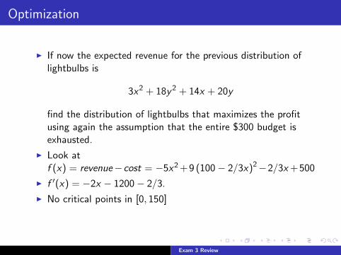
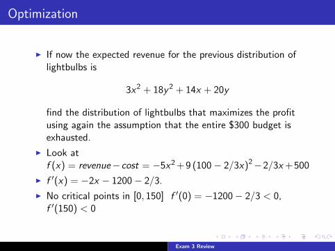
I If now the expected revenue for the previous distribution oflightbulbs is
3x2 + 18y2 + 14x + 20y
find the distribution of lightbulbs that maximizes the profitusing again the assumption that the entire $300 budget isexhausted.
I Look atf (x) = revenue−cost = −5x2 + 9 (100− 2/3x)2−2/3x + 500
I f ′(x) = −2x − 1200− 2/3.
I No critical points in [0, 150] f ′(0) = −1200− 2/3 < 0,f ′(150) < 0 (or f (0) = 90500, f (150) = −110600).
Exam 3 Review

Optimization
I If now the expected revenue for the previous distribution oflightbulbs is
3x2 + 18y2 + 14x + 20y
find the distribution of lightbulbs that maximizes the profitusing again the assumption that the entire $300 budget isexhausted.
I Look atf (x) = revenue−cost = −5x2 + 9 (100− 2/3x)2−2/3x + 500
I f ′(x) = −2x − 1200− 2/3.
I No critical points in [0, 150] f ′(0) = −1200− 2/3 < 0,f ′(150) < 0 (or f (0) = 90500, f (150) = −110600).
Exam 3 Review
Optimization
I If now the expected revenue for the previous distribution oflightbulbs is
3x2 + 18y2 + 14x + 20y
find the distribution of lightbulbs that maximizes the profitusing again the assumption that the entire $300 budget isexhausted.
I Look atf (x) = revenue−cost = −5x2 + 9 (100− 2/3x)2−2/3x + 500
I f ′(x) = −2x − 1200− 2/3.
I No critical points in [0, 150]
f ′(0) = −1200− 2/3 < 0,f ′(150) < 0 (or f (0) = 90500, f (150) = −110600).
Exam 3 Review

Optimization
I If now the expected revenue for the previous distribution oflightbulbs is
3x2 + 18y2 + 14x + 20y
find the distribution of lightbulbs that maximizes the profitusing again the assumption that the entire $300 budget isexhausted.
I Look atf (x) = revenue−cost = −5x2 + 9 (100− 2/3x)2−2/3x + 500
I f ′(x) = −2x − 1200− 2/3.
I No critical points in [0, 150] f ′(0) = −1200− 2/3 < 0,
f ′(150) < 0 (or f (0) = 90500, f (150) = −110600).
Exam 3 Review
Optimization
I If now the expected revenue for the previous distribution oflightbulbs is
3x2 + 18y2 + 14x + 20y
find the distribution of lightbulbs that maximizes the profitusing again the assumption that the entire $300 budget isexhausted.
I Look atf (x) = revenue−cost = −5x2 + 9 (100− 2/3x)2−2/3x + 500
I f ′(x) = −2x − 1200− 2/3.
I No critical points in [0, 150] f ′(0) = −1200− 2/3 < 0,f ′(150) < 0
(or f (0) = 90500, f (150) = −110600).
Exam 3 Review

Optimization
I If now the expected revenue for the previous distribution oflightbulbs is
3x2 + 18y2 + 14x + 20y
find the distribution of lightbulbs that maximizes the profitusing again the assumption that the entire $300 budget isexhausted.
I Look atf (x) = revenue−cost = −5x2 + 9 (100− 2/3x)2−2/3x + 500
I f ′(x) = −2x − 1200− 2/3.
I No critical points in [0, 150] f ′(0) = −1200− 2/3 < 0,f ′(150) < 0 (or f (0) = 90500, f (150) = −110600).
Exam 3 Review

Other Optimization Problems
I Suppose that a cost function is given by
c(x) = 2x2 +3x
1 + xfor x > 0
Minimize the average cost.
I What if now
c(x) =xe−2x
1 + x2?
Exam 3 Review

Other Optimization Problems
I Suppose that a cost function is given by
c(x) = 2x2 +3x
1 + xfor x > 0
Minimize the average cost.
I What if now
c(x) =xe−2x
1 + x2?
Exam 3 Review

Other Optimization Problems
I Suppose that a cost function is given by
c(x) = 2x2 +3x
1 + xfor x > 0
Minimize the average cost.
I What if now
c(x) =xe−2x
1 + x2?
Exam 3 Review

Other Optimization Problems
I Suppose that a cost function is given by
c(x) = 2x2 +3x
1 + xfor x > 0
Minimize the average cost.
I What if now
c(x) =xe−2x
1 + x2?
Exam 3 Review

Other Optimization Problems
I Suppose that a cost function is given by
c(x) = 2x2 +3x
1 + xfor x > 0
Minimize the average cost.
I What if now
c(x) =xe−2x
1 + x2?
Exam 3 Review

Compounded Interest
I Interest compounded periodically
A︸︷︷︸Accumulated Amount
= P︸︷︷︸Principal
(1 + r/m)mt
I r Interest rate,
I Divide the year into m periods of equal duration
I t = # of years
I Continuous compounding od interest A = Pert .
I Initial capital from accumulated amount: P = A(1 + r
m
)−mt.
Exam 3 Review
Compounded Interest
I Interest compounded periodically
A︸︷︷︸Accumulated Amount
= P︸︷︷︸Principal
(1 + r/m)mt
I r Interest rate,
I Divide the year into m periods of equal duration
I t = # of years
I Continuous compounding od interest A = Pert .
I Initial capital from accumulated amount:
P = A(1 + r
m
)−mt.
Exam 3 Review

Compounded Interest
I Interest compounded periodically
A︸︷︷︸Accumulated Amount
= P︸︷︷︸Principal
(1 + r/m)mt
I r Interest rate,
I Divide the year into m periods of equal duration
I t = # of years
I Continuous compounding od interest A = Pert .
I Initial capital from accumulated amount: P = A(1 + r
m
)−mt.
Exam 3 Review

Curve sketching
I Steps
1. Find and classify critical points2. Points where the function is increasing/decreasing3. Inflection points (change in convexity/concavity).4. Horizontal Asymptotes/Vertical Asymptotes.
Iex
xI e−(x−3)(x−5)
Exam 3 Review

Curve sketching
I Steps
1. Find and classify critical points2. Points where the function is increasing/decreasing3. Inflection points (change in convexity/concavity).4. Horizontal Asymptotes/Vertical Asymptotes.
Iex
xI e−(x−3)(x−5)
Exam 3 Review

Curve sketching
I Steps
1. Find and classify critical points
2. Points where the function is increasing/decreasing3. Inflection points (change in convexity/concavity).4. Horizontal Asymptotes/Vertical Asymptotes.
Iex
xI e−(x−3)(x−5)
Exam 3 Review

Curve sketching
I Steps
1. Find and classify critical points2. Points where the function is increasing/decreasing
3. Inflection points (change in convexity/concavity).4. Horizontal Asymptotes/Vertical Asymptotes.
Iex
xI e−(x−3)(x−5)
Exam 3 Review

Curve sketching
I Steps
1. Find and classify critical points2. Points where the function is increasing/decreasing3. Inflection points (change in convexity/concavity).
4. Horizontal Asymptotes/Vertical Asymptotes.
Iex
xI e−(x−3)(x−5)
Exam 3 Review

Curve sketching
I Steps
1. Find and classify critical points2. Points where the function is increasing/decreasing3. Inflection points (change in convexity/concavity).4. Horizontal Asymptotes/Vertical Asymptotes.
Iex
xI e−(x−3)(x−5)
Exam 3 Review

Curve sketching
I Steps
1. Find and classify critical points2. Points where the function is increasing/decreasing3. Inflection points (change in convexity/concavity).4. Horizontal Asymptotes/Vertical Asymptotes.
Iex
x
I e−(x−3)(x−5)
Exam 3 Review
Curve sketching
I Steps
1. Find and classify critical points2. Points where the function is increasing/decreasing3. Inflection points (change in convexity/concavity).4. Horizontal Asymptotes/Vertical Asymptotes.
Iex
xI e−(x−3)(x−5)
Exam 3 Review