Evidence and scenario sensitivities in nave Bayesian classifiersPresented byMarwan Kandela & Rejin James *Silja Renooij, Linda C. van der Gaag, "Evidence and scenario sensitivities in naive Bayesian classifiers," International Journal of Approximate Reasoning, Volume 49, Issue 2, October 2008, Pages 398-416, ISSN 0888-613X, 10.1016/j.ijar.2008.02.008. (http://www.sciencedirect.com/science/article/pii/S0888613X08000236)

AuthorsProfessors at the University of Utrecht (The Netherlands).Department of Information and Computing Sciences.Many publications together, Papers (peer reviewed), Journals etcConference/Workshop

Silja RenooijLinda C. van der Gaag*

IntroductionWhat is a Classifier ?It is an Algorithm that Classifies a new observation to one category in a set of categories.What is a Feature ? The individual Observations are analyzed into a set of quantifiable properties known as Features.

*

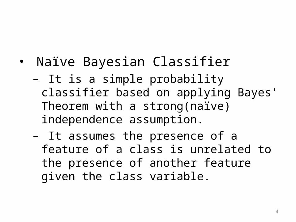
Nave Bayesian Classifier It is a simple probability classifier based on applying Bayes' Theorem with a strong(nave) independence assumption. It assumes the presence of a feature of a class is unrelated to the presence of another feature given the class variable. *

*

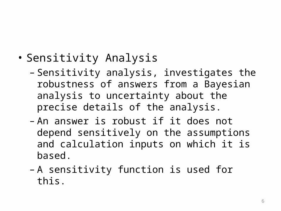
Sensitivity AnalysisSensitivity analysis, investigates the robustness of answers from a Bayesian analysis to uncertainty about the precise details of the analysis. An answer is robust if it does not depend sensitively on the assumptions and calculation inputs on which it is based.A sensitivity function is used for this. *

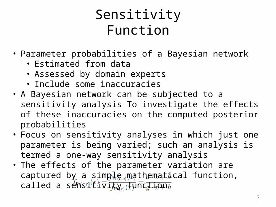
Sensitivity FunctionParameter probabilities of a Bayesian network Estimated from dataAssessed by domain expertsInclude some inaccuraciesA Bayesian network can be subjected to a sensitivity analysis To investigate the effects of these inaccuracies on the computed posterior probabilitiesFocus on sensitivity analyses in which just one parameter is being varied; such an analysis is termed a one-way sensitivity analysisThe effects of the parameter variation are captured by a simple mathematical function, called a sensitivity function

*

A one-way sensitivity function f(x) can take one of three general forms. It is linear if:The probability of interest is a prior probability rather than a posterior probabilityThe probability of the entered evidence is unaffected by the parameter variationIn the other two cases the sensitivity function is a fragment of a rectangular hyperbola, which takes the general form

We will focus on this last type of function and assume any sensitivity function to be hyperbolic unless explicitly stated otherwise. As we all know a rectangular hyperbola in general has two branches and two asymptotes defining its center (s,t)The equation above could be used to calculate the values we may need

Sensitivity Function*

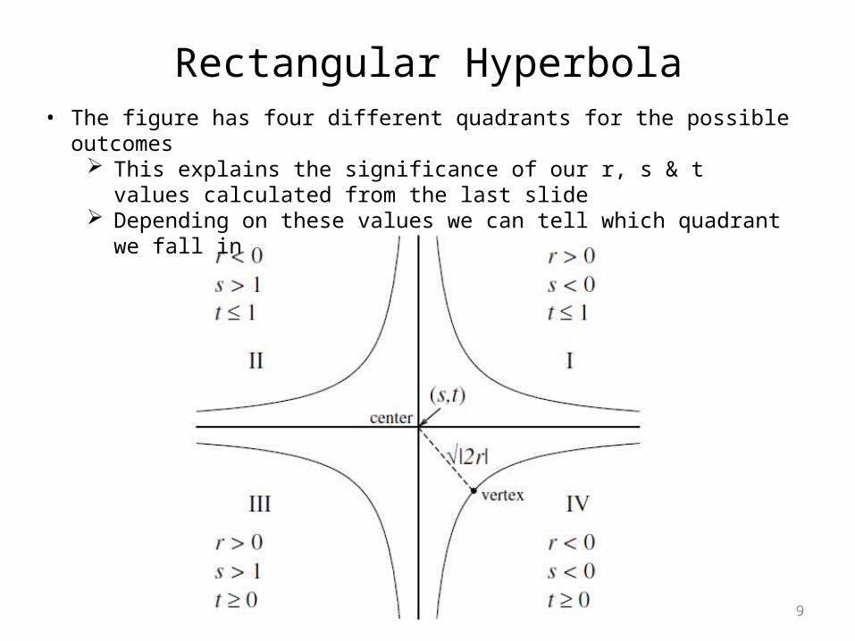
Rectangular HyperbolaThe figure has four different quadrants for the possible outcomesThis explains the significance of our r, s & t values calculated from the last slideDepending on these values we can tell which quadrant we fall in*

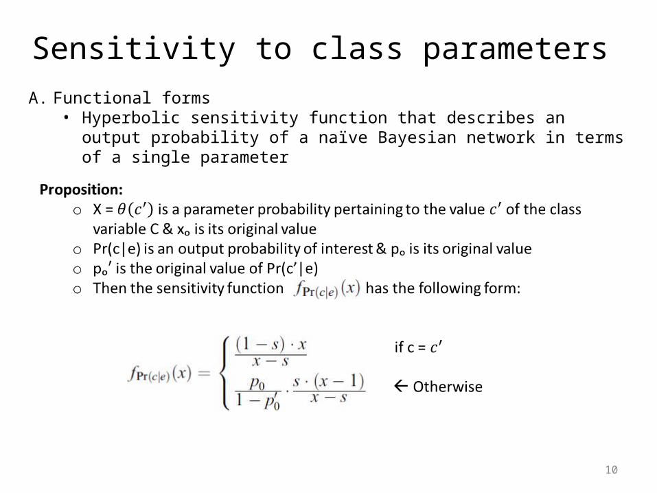
Sensitivity to class parametersFunctional formsHyperbolic sensitivity function that describes an output probability of a nave Bayesian network in terms of a single parameter

*

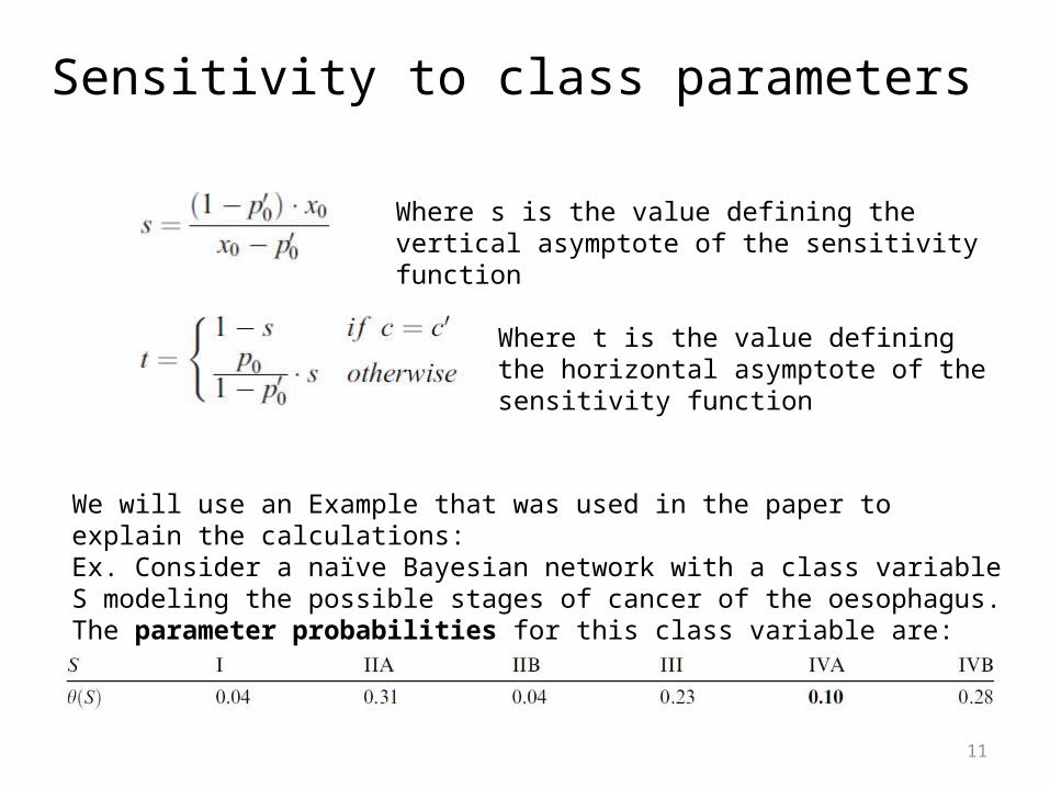
Sensitivity to class parametersWhere s is the value defining the vertical asymptote of the sensitivity functionWhere t is the value defining the horizontal asymptote of the sensitivity functionWe will use an Example that was used in the paper to explain the calculations:Ex. Consider a nave Bayesian network with a class variable S modeling the possible stages of cancer of the oesophagus. The parameter probabilities for this class variable are:*

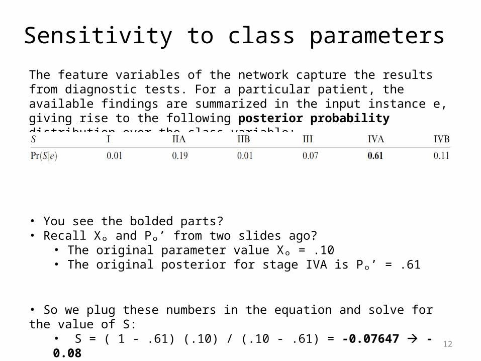
Sensitivity to class parametersThe feature variables of the network capture the results from diagnostic tests. For a particular patient, the available findings are summarized in the input instance e, giving rise to the following posterior probability distribution over the class variable:

You see the bolded parts? Recall X and P from two slides ago? The original parameter value X = .10 The original posterior for stage IVA is P = .61

So we plug these numbers in the equation and solve for the value of S: S = ( 1 - .61) (.10) / (.10 - .61) = -0.07647 -0.08 The sensitivity function therefore is a fourth quadrant hyperbola branch. why do we say so? How do we know?*

Sensitivity to class parametersWe have no need to perform any more computations or calculate anything else. We can establish the equations we need:

We observe that the functions are fully determined by just the original value for the class parameter being varied and the original posterior probability distribution over the output variable of interest.

Any questions about the Calculations?

*

Sensitivity to class parametersB. Sensitivity properties Any sensitivity property pertaining to a class parameter can be computed from the sensitivity function we derived in the last slide. That is why this paper also makes sure to go over the sensitivity value and admissible deviation.

Sensitivity Value* By expressing the output probability in terms of a class parameter from the sensitivity function the following equation is readily established:

Now we will use different combinations of X and P to compute sensitivity values from this function and plot them into a graph.*

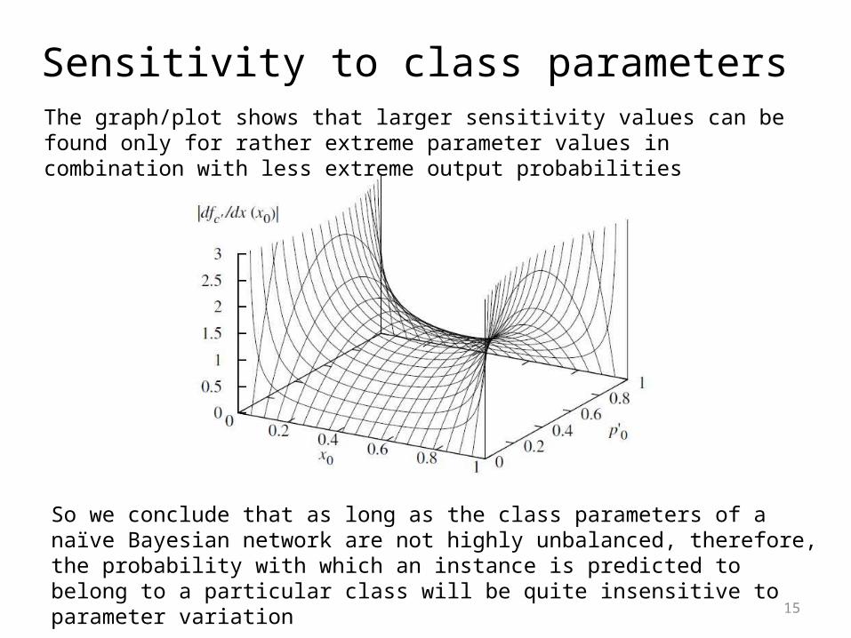
Sensitivity to class parametersThe graph/plot shows that larger sensitivity values can be found only for rather extreme parameter values in combination with less extreme output probabilitiesSo we conclude that as long as the class parameters of a nave Bayesian network are not highly unbalanced, therefore, the probability with which an instance is predicted to belong to a particular class will be quite insensitive to parameter variation*

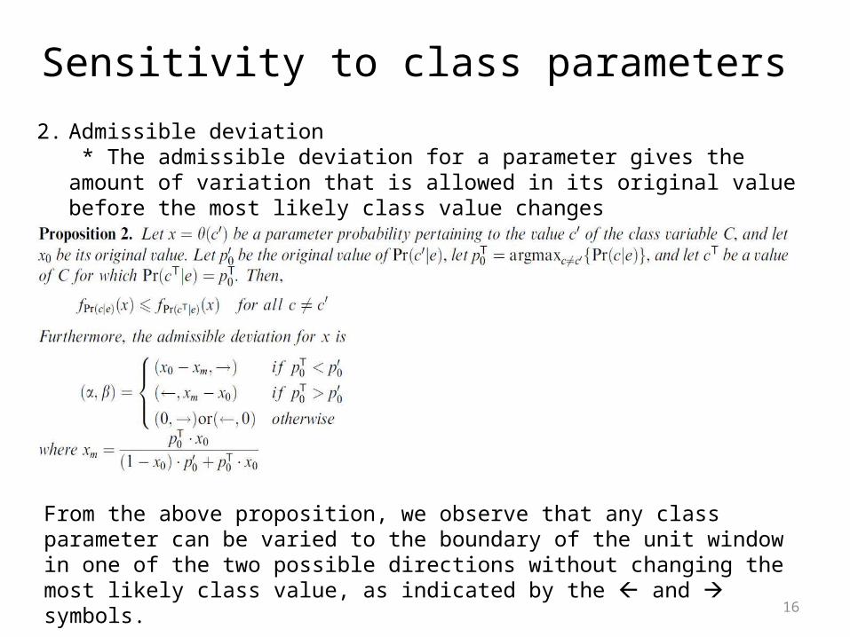
Sensitivity to class parametersAdmissible deviation * The admissible deviation for a parameter gives the amount of variation that is allowed in its original value before the most likely class value changesFrom the above proposition, we observe that any class parameter can be varied to the boundary of the unit window in one of the two possible directions without changing the most likely class value, as indicated by the and symbols.*

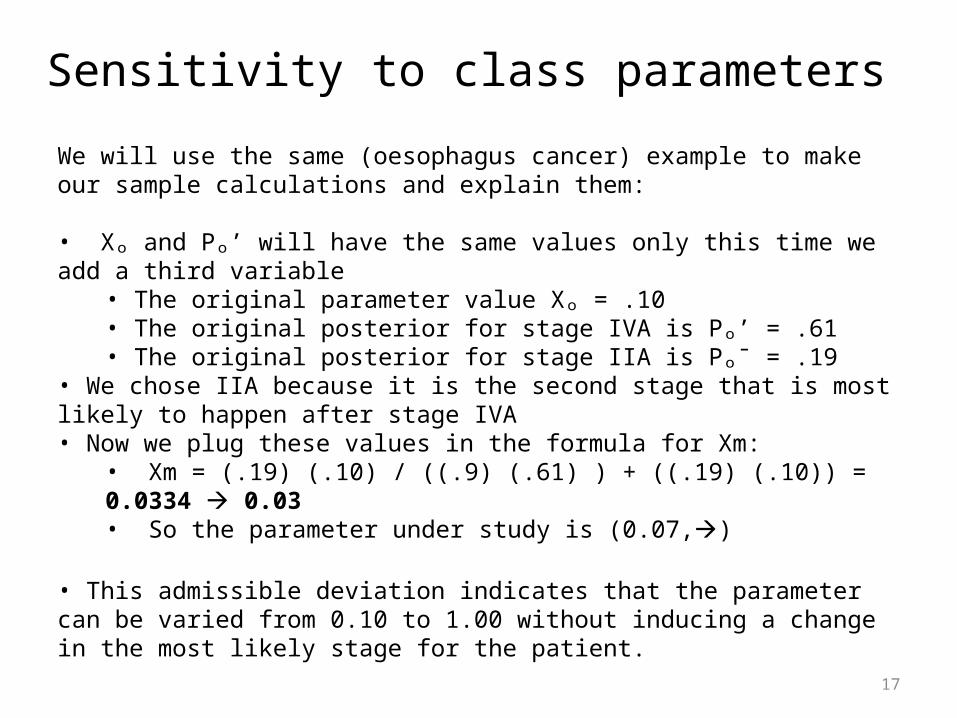
Sensitivity to class parametersWe will use the same (oesophagus cancer) example to make our sample calculations and explain them:

X and P will have the same values only this time we add a third variable The original parameter value X = .10 The original posterior for stage IVA is P = .61 The original posterior for stage IIA is P = .19 We chose IIA because it is the second stage that is most likely to happen after stage IVA Now we plug these values in the formula for Xm: Xm = (.19) (.10) / ((.9) (.61) ) + ((.19) (.10)) = 0.0334 0.03 So the parameter under study is (0.07,)

This admissible deviation indicates that the parameter can be varied from 0.10 to 1.00 without inducing a change in the most likely stage for the patient.

*

Sensitivity to feature parametersFunctional formsHyperbolic sensitivity function that describes an output probability of a nave Bayesian network in terms of a single parameter*

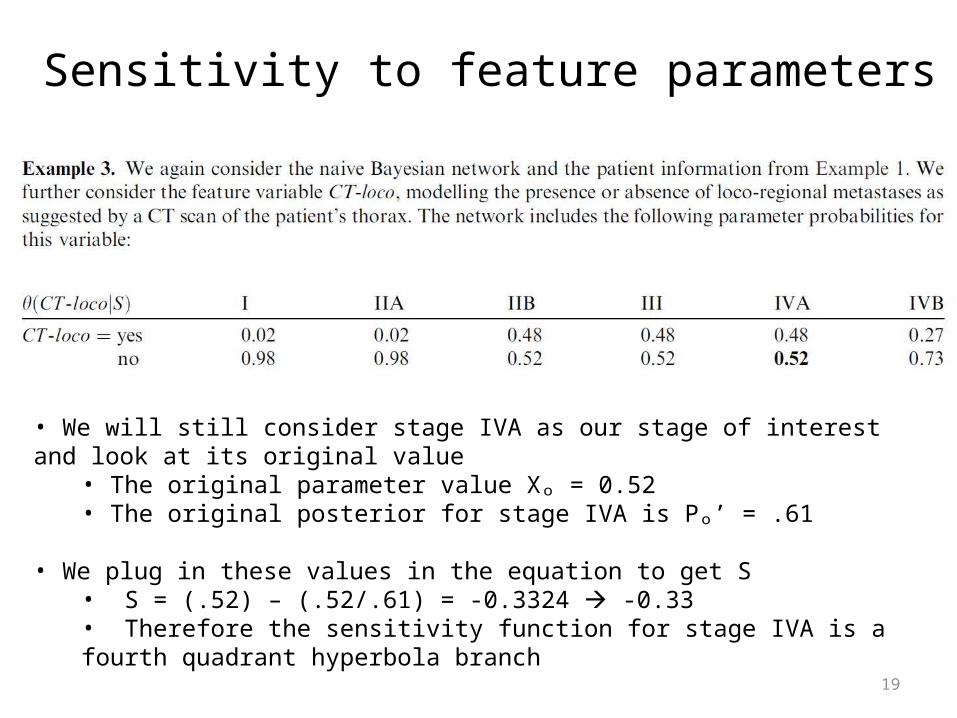
Sensitivity to feature parameters We will still consider stage IVA as our stage of interest and look at its original value The original parameter value X = 0.52 The original posterior for stage IVA is P = .61

We plug in these values in the equation to get S S = (.52) (.52/.61) = -0.3324 -0.33 Therefore the sensitivity function for stage IVA is a fourth quadrant hyperbola branch

*

Sensitivity to feature parametersWithout performing any further computations we establish thatJust as the sensitivity functions for the class parameters, we find that the functions for the feature parameters are exactly determined by the original values for these parameters and the original posterior probability distribution for the output variable of interest.

Sensitivity propertiesAny sensitivity property pertaining to a networks feature parameters can be computedStudy the properties of sensitivity value and admissible deviation*

Sensitivity to feature parametersSensitivity Value* By expressing the output probability in terms of a feature parameter from the sensitivity function the following sensitivity value is readily established:Now we will use different combinations of X and P to compute sensitivity values from this function and plot them into a graph.*

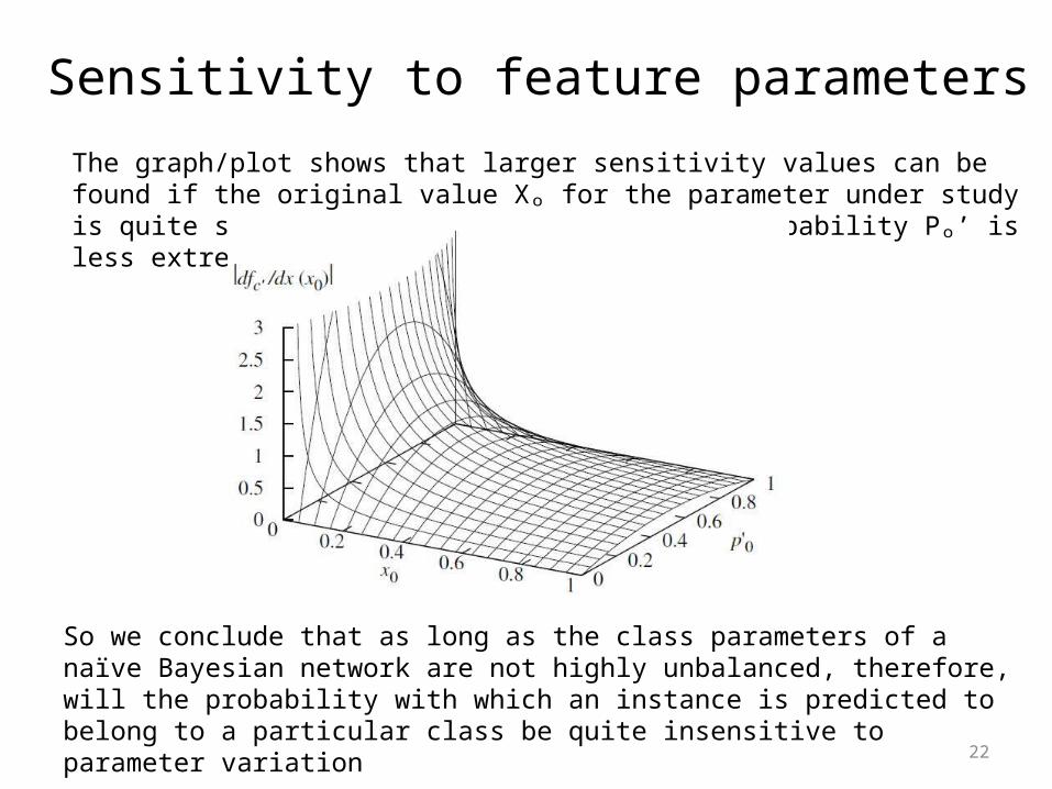
The graph/plot shows that larger sensitivity values can be found if the original value X for the parameter under study is quite small and the original posterior probability P is less extreme Sensitivity to feature parametersSo we conclude that as long as the class parameters of a nave Bayesian network are not highly unbalanced, therefore, will the probability with which an instance is predicted to belong to a particular class be quite insensitive to parameter variation*

Admissible deviation * The admissible deviation for a parameter gives the amount of variation that is allowed in its original value before the most likely class value changes Sensitivity to feature parameters*

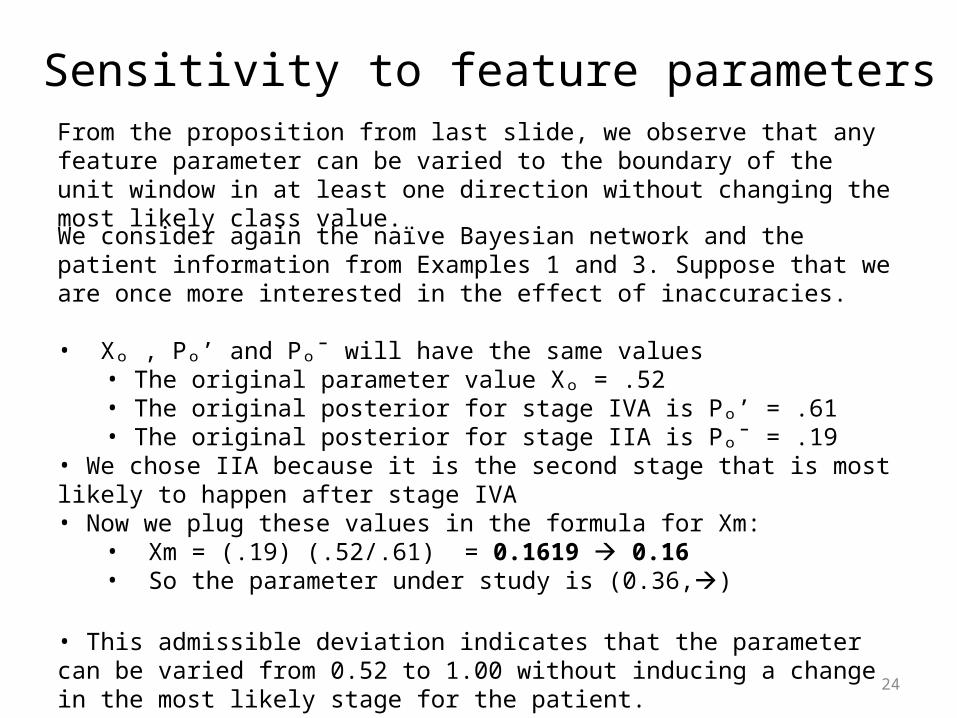
From the proposition from last slide, we observe that any feature parameter can be varied to the boundary of the unit window in at least one direction without changing the most likely class value. Sensitivity to feature parametersWe consider again the nave Bayesian network and the patient information from Examples 1 and 3. Suppose that we are once more interested in the effect of inaccuracies.

X , P and P will have the same values The original parameter value X = .52 The original posterior for stage IVA is P = .61 The original posterior for stage IIA is P = .19 We chose IIA because it is the second stage that is most likely to happen after stage IVA Now we plug these values in the formula for Xm: Xm = (.19) (.52/.61) = 0.1619 0.16 So the parameter under study is (0.36,)

This admissible deviation indicates that the parameter can be varied from 0.52 to 1.00 without inducing a change in the most likely stage for the patient.*

Scenario Sensitivity Scenario sensitivity means sensitivity to the scenarios with possibly additional evidence.

Here scenario sensitivities are discussed in the context of a nave Bayesian Network.

In this section the authors trys to figure out - how much impact additional evidence could have on the probability distribution over the class variable and -how sensitive this impact is to the inaccuracies in the networks parameters.

*

First We try to figure out the impact of additional evidence on an output probability of interest For this a ratio is consideredLet E and E be a set of feature variables

Where, E E Eand E- E={E ,E l} , 1 l n

Let e and e be the instancesThen, for each class value c

-> posterior probability prior to obtaining new information Scenario Sensitivity*

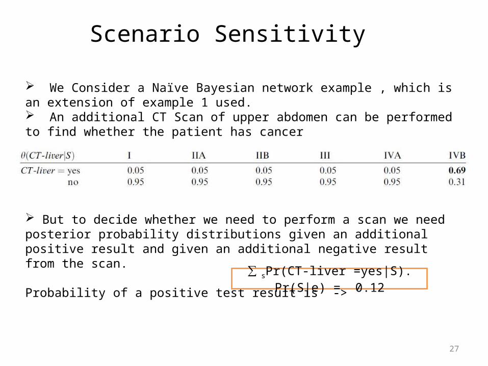
Scenario Sensitivity We Consider a Nave Bayesian network example , which is an extension of example 1 used. An additional CT Scan of upper abdomen can be performed to find whether the patient has cancer

But to decide whether we need to perform a scan we need posterior probability distributions given an additional positive result and given an additional negative result from the scan.

Probability of a positive test result is ->

sPr(CT-liver =yes|S). Pr(S|e) = 0.12*

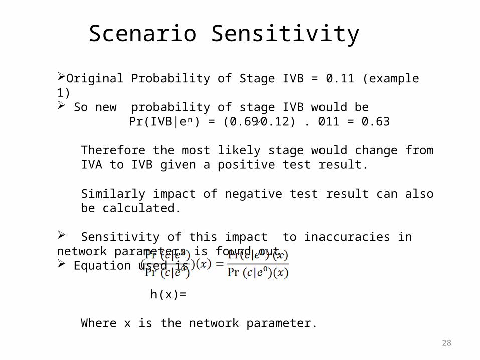
Original Probability of Stage IVB = 0.11 (example 1) So new probability of stage IVB would be Pr(IVB|e) = (0.690.12) . 011 = 0.63

Therefore the most likely stage would change from IVA to IVB given a positive test result.

Similarly impact of negative test result can also be calculated.

Sensitivity of this impact to inaccuracies in network parameters is found out. Equation used is h(x)=

Where x is the network parameter.

Scenario Sensitivity *

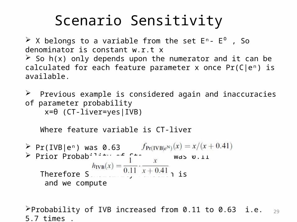
Scenario Sensitivity X belongs to a variable from the set E- E , So denominator is constant w.r.t x So h(x) only depends upon the numerator and it can be calculated for each feature parameter x once Pr(C|e) is available.

Previous example is considered again and inaccuracies of parameter probability x= (CT-liver=yes|IVB)

Where feature variable is CT-liver

Pr(IVB|e) was 0.63 Prior Probability of Stage IVB was 0.11

Therefore Sensitivity Function is and we compute

Probability of IVB increased from 0.11 to 0.63 i.e. 5.7 times . If x is varied, IVB becomes at most 6.4 times.

*

Conclusion Sensitivity-analysis techniques used to study effects of parameter inaccuracies on the posterior probability distributions from a naive Bayesian network. Sensitivity parameters determined solely by the original value of the parameter under study and Posterior Probability distribution. Properties Help us to study robustness of nave Bayesian Classifier. A novel notion of scenario sensitivity was introduced Scenario sensitivities expressed in terms of standard sensitivity functions Future work -> to study the properties of scenario sensitivity functions for all classifier parameters and Bayesian Networks in General*

Rejin James and Marwan Kandela, April 19, 2012: Silja Renooij, Linda C. van der Gaag, "Evidence and scenario sensitivities in naive Bayesian classifiers," International Journal of Approximate Reasoning, Volume 49, Issue 2, October 2008, Pages 398-416, ISSN 0888-613X, 10.1016/j.ijar.2008.02.008. (http://www.sciencedirect.com/science/article/pii/S0888613X08000236)****