Electronic copy available at: http://ssrn.com/abstract=1752115

Everything You Always Wanted to Know about Log Periodic

Power Laws for Bubble Modelling but Were Afraid to Ask

Petr Geraskin∗

Dean Fantazzini†

Abstract

Sornette et al. (1996), Sornette and Johansen (1997), Johansen et al. (2000)and Sornette (2003a) proposed that, prior to crashes, the mean function of a stockindex price time series is characterized by a power law decorated with log-periodicoscillations, leading to a critical point that describes the beginning of the marketcrash. This paper reviews the original Log-Periodic Power Law (LPPL) model forfinancial bubble modelling, and discusses early criticism and recent generalizationsproposed to answer these remarks. We show how to fit these models with alternativemethodologies, together with diagnostic tests and graphical tools to diagnose financialbubbles in the making in real time. An application of this methodology to the Goldbubble which busted in December 2009 is then presented.

Keywords: Log-periodic models, LPPL, Crash, Bubble, Anti-Bubble, GARCH,Forecasting, Gold.

JEL classification: C32, C51, C53, G17.

∗Higher School of Economics, Moscow, Russia. E-mail: petr-geraskin@mail.ru†Moscow School of Economics - Moscow State University (Russia);

Faculty of Economics - Higher School of Economics (Moscow, Russia);The International College of Economics and Finance - Higher School of Economics (Moscow, Russia);E-mail: fantazzini@mse-msu.ru

This is the working paper version of the paper Everything You Always Wanted to Know about Log Periodic

Power Laws for Bubble Modelling but Were Afraid to Ask, forthcoming in the European Journal of Finance.

1

Electronic copy available at: http://ssrn.com/abstract=1752115

1 Introduction

Detecting a financial bubble and predicting when it will end has become of crucial im-

portance, given the series of financial bubbles that led to the current "Second Great

Contraction", using the definition by Reinhart and Rogoff (2009). As noted by Sornette

(2009), Sornette and Woodard (2010), Kaizoji and Sornette (2010), Sornette et al. (2009)

and Fantazzini (2010a,b), the global financial crisis that has started in 2007 can be con-

sidered an example of how the bursting of a bubble can be dealt with by creating new

bubbles. This consideration which is not new in the financial literature, see e.g. Sornette

and Woodard (2010) and references therein, was indirectly confirmed by Lou Jiwei, the

chairman of the $298 billion sovereign wealth fund named China Investment Corporation

(CIC), which was created in 2007 with the goal to manage an important part of the Peo-

ple’s Republic of China’s foreign exchange reserves. On August the 28th 2009, Lou told

reporters on the sidelines of a forum organized by the Washington-based Brookings In-

stitution and the Chinese ’Economists 50 Forum’, a Beijing think-tank, that "both China

and America are addressing bubbles by creating more bubbles and we’re just taking ad-

vantage of that. So we can’t lose". Moreover, Lou also added that "CIC was building

a broad investment portfolio that includes products designed to generate both alpha and

beta; to hedge against both inflation and deflation; and to provide guaranteed returns in

the event of a new crisis". See the full Reuters article by Zhou Xin and Alan Wheatley at

http://www.reuters.com/article/ousiv/idUSTRE57S0D420090829 for more details. The

previous comments clearly point out how important is to have tools able to detect bubbles

in the making.

Unfortunately, there is no consensus in the economic literature on what a bubble is:

Gurkaynak (2008) surveyed a large set of econometric tests of asset price bubbles and

found that for each paper that finds evidence of bubbles, there is another one that fits

the data equally well without allowing for a bubble, so that it is not possible to distin-

guish bubbles from time-varying fundamentals. A similar situation can also be found in

the professional literature: for example, Alan Greenspan stated on August the 30th 2002

that " ...We, at the Federal Reserve ... recognized that, despite our suspicions, it was

very difficult to definitively identify a bubble until after the fact, that is, when its bursting

2

confirmed its existence". So, is this a lost cause? Absolutely not.

A model which has quickly gained a lot of attention among financial practitioners and in

the Physics academic literature due to the many successful predictions, is the so called Log

Periodic Power Law (LPPL) approach proposed by Johansen et al. (2000) and Sornette

(2003a,b). The Johansen-Ledoit-Sornette (JLS) model assumes the presence of two types

of agents in the market: a group of traders with rational expectations and a second group

of so called "noise" traders, that is irrational agents with herding behavior. The idea of

the JLS model comes from statistical physics and it shares many elements with a model

introduced by Ising for explaining ferromagnetism, see e.g. Goldenfeld (1992). According

to this model, traders are organized into networks and can have only two states: buy or

sell. In addition, their trading actions depend on the decisions of other traders and on

external influences. Due to these interactions, agents can form groups with self-similar

behavior which can lead the market to a bubble situation, which can be considered a

situation of "order", compared to the "disorder" of normal market conditions. Another

important feature introduced in this model is the positive feedbacks which are generated

by the increasing risk and the agents’ interactions, so that a bubble can be a self-sustained

process.

Many examples of calibrations of financial bubbles with LPPLs are reported in Sornette

(2003a), who suggests that the LPPL model provides a good starting point to detect

bubbles and forecast their most probable end. Johansen and Sornette (2004) identified

the most extreme cumulative losses (i.e. drawdowns) in a large set of financial assets

and showed that they belong to a probability density distribution, which is distinct from

the distribution of the 99% of the smaller drawdowns which represent the normal market

regime. Moreover, they showed that, for two-third of these extreme drawdowns, the market

prices followed a super-exponential behavior prior to their occurrences, as confirmed by a

calibration of a LPPL model. These particular drawdowns (or outliers) are called "dragon

kings" in Sornette (2009). Interestingly, this approach allowed to diagnose bubbles ex-ante,

as shown in a series of real-life tests, see Sornette and Zhou (2006), Sornette, Woodard and

Zhou (2008) and Zhou and Sornette (2003, 2006, 2008, 2009). Furthermore, it is currently

being used at the Financial Crisis Observatory (FCO), which is a scientific platform set

3

up at the ETH - Zurich, aimed at "testing and quantifying rigorously the hypothesis that

financial markets exhibit a degree of inefficiency and a potential for predictability, especially

during regimes when bubbles develop", see http://www.er.ethz.ch/fco for more details.

The goal of this paper is to present an easy-to-use and self-contained guide for bubble

modelling and detecting with Log Periodic Power Laws, which contains all the sufficient

steps to derive the main models in this growing and interesting field of the literature, and

discusses the important aspects for practitioners and researchers.

The rest of the paper is organized as follows. Section 2 reviews the original JLS model

with the main steps required for its derivation. Section 3 discusses the early criticism

to this approach and recent generalizations proposed to answer these remarks. Section

4 discusses how to fit LPPLs models, by presenting three estimation methodologies: the

original 2-step nonlinear optimization by Johansen et al. (2000), the Genetic Algorithm

approach proposed by Jacobsson (2009) and the 2-step/3-step ML approach proposed

by Fantazzini (2010a). Section 5 is devoted to the diagnosis of bubbles in the making

by using a set of different techniques. We describe diagnostic tests based on the LPPL

fitting residuals, diagnostic tests based on rational expectation models with stochastic

mean-reverting termination times, as well as graphical tools useful for capturing bubble

development and for understanding whether a crash is in sight or not. Section 6 presents a

detailed empirical application devoted to the burst of the gold bubble in December 2009,

while Section 7 briefly concludes.

2 The Original LPPL model

Johansen et al. (JLS, 2000) consider an ideal market with no dividends, and where in-

terest rates, risk aversion and market liquidity constraints are ignored. Therefore, the

fundamental value for an asset is p(t) = 0, so any positive value of p(t) represents a bub-

ble. In general, p(t) can be viewed as the price in excess of the fundamental value of an

asset. In this framework, there are two types of agents: first, a group of rational agents

who are identical in their preferences and characteristics, so they can be substituted with

a single representative agent. Second, a group of irrational agents whose herding behavior

leads to the development of a financial bubble. When this tendency develops till a certain

4

critical value, a large proportion of agents will then assume the same short position, thus

causing a crash. A financial crash is not a certain event in this model, but it is character-

ized by a probability distribution: as a consequence, it is rational for financial agents to

continue investing, because the risk of the crash to happen is compensated by the positive

return generated by the financial bubble and there exists a small probability for the bubble

to disappear smoothly, without the occurrence of a crash.

The key variable to model the price behavior before a crash is the crash hazard rate h(t),

that is the probability per unit of time that the crash will take place, given that it has not

yet occurred. The hazard rate h(t) quantifies the probability that a great number of agents

will assume the same sell position simultaneously, a position that the market will not be

able to satisfy unless the prices decrease substantially. We remark that in this model a

strong collective answer (as it is the case for a crash) is not necessarily the consequence of

one elaborated internal mechanism of global coordination, but it can appear starting from

imitative local micro-interactions which are then transmitted by the market resulting in

a macroscopic effect. In this regard, JLS (2000) first discuss a macroscopic "mean field"

approach and then turn to a more microscopic approach.

2.1 Macroscopic Modelling

According to the mean field theory from Statistical Mechanics (see e.g. Stanley (1971)

and Goldenfeld, (1992)), a simple way for describing an imitative process is by assuming

that the hazard rate h(t) can be described by the following equation:

dh

dt= Chδ (1)

where C > 0 is a constant, and δ > 1 represents the average number of interactions among

traders minus one. Thus, it follows that an amplification of interactions increases the

hazard rate. If we integrate (1), we have:

h(t) =

(

h0

tc − t

)α

, α =1

δ − 1(2)

where tc is the critical time determined by the initial conditions at some origin of time.

It can be shown that the condition δ > 1 (and consequently α > 0) is crucial to obtain a

growth of h(t) as t→ tc and therefore a critical point in finite time. Moreover, the condition

5

that α < 1 is required for the price not to diverge at tc. Rewriting these condition for δ

we have that 2 < δ <∞, that is, an agent should be connected at least with two agents.

Another important feature of this approach is the possibility of self-fulfilling crisis, which

is a concept recently proposed to explain the recession in the ’90 in seven countries (Ar-

gentina, Indonesia, Hong Kong, Malaysia, Mexico, South Korea and Thailand), see Krug-

man (1998) and Sornette (2003a). It is suggested that the loss of investor’s confidence

caused a self-fulfilling process in these countries and thus led to severe recessions. This

feedback process can be modelled by using the previous mean field approach:

dh

dt= Dpµ, µ > 0 (3)

whereD is a positive constant. The underlying idea is that the lack of confidence quantified

by the hazard rate increases when the market price departs from its fundamental value.

Therefore, the price has to increase to compensate the increasing risk.

2.2 Microscopic Modelling

JLS (2000) and Sornette (2003a) assume that the group of irrational agents are connected

into a network. Each agent is indexed by a integer number i = 1, . . . , I and N(i) represents

the number of agents who are directly connected to agent i in the network. JLS (2000)

assume that each agent can have only two possible states si: "buy" (si = +1) or "sell"

(si = −1). JLS (2000) suppose that the state of agent i is determined by the following

Markov process:

si = sign

K∑

k∈N(i)

sj + σεi

(4)

where the sign function sign(x) is equal to +1 if x > 0 and to −1 if x < 0, K is a positive

constant, εi is an i.i.d. standard normal random variable. In this model, K governs the

tendency of imitation among traders, while σ governs their idiosyncratic behavior. If K

increases, the order in the network increases as well, while the reverse is true when σ

increases. If order wins, the agents will imitate their close neighbors and their imitation

will spread all over the network, thus causing a crash1. More specifically and in analogy

1In the context of the alignment of atomic spins to create magnetization, this model represented by (4)is identical to the so-called two-dimensional Ising model which was solved explicitly by Onsager (1944),and where the disorder parameter is represented by the temperature of the system.

6

with the Ising model, there exists a critical point Kc, that determines the separation

between the different regimes: when K < Kc the disorder reigns and the sensibility to

a small global influence is low. When the imitation force K grows approaching Kc, a

hierarchy of groups of agents acting collectively and with the same position is formed.

As a consequence, the market becomes extremely sensitive to small global disturbances.

Finally, for a larger imitation force so that K > Kc, the tendency of imitation is so intense

that there exists a strong predominance of one state/position among agents.

A physical quantity that represent the degree of a system sensitivity to an external per-

turbation (or general global influence) is the so-called susceptibility of the system. This

quantity describes the probability that a large group of agents will have the same state,

given the existent external influences in the network. Let us assume the existence of a

term G which measures the global influence, and add it to (4):

si = sign

K∑

k∈N(i)

sj + σεi +G

(5)

If we define the average state of the market as M = (1/I)∑I

i=1 si, for G = 0 we have

E[M ] = 0 by symmetry. For G > 0, we have M > 0, while for G < 0, M < 0. Thus, it fol-

lows that E[M ]×G ≥ 0. The susceptibility of the system is then defined as χ = dE[M ]dG

∣

∣

∣

G=0.

In general, the susceptibility has three possible interpretations: first, it measures the sen-

sitivity of M to a small change in the global influence. Secondly, it is (a constant times)

the variance of M around its zero expectation, caused by idiosyncratic shocks εi. Finally,

if we consider two agents and we force one to be in a certain state, the impact that our

intervention will have on the second agent will be proportional to the susceptibility.

2.3 Price Dynamics and Derivation of the JLS Model

As previously anticipated, the rational agent considered by JLS (2000) is risk neutral

and has rational expectations. Thus, the asset price p(t) follows a martingale process,

i.e. Et[p(t′)] = p(t), ∀t′ > t, where Et[.] represents the conditional expectation given all

information available up to time t. In the case of market equilibrium, the previous equality

is a necessary condition for no arbitrage.

Considering that there exists a not zero probability for the crash to happen, we can define

7

a jump process j which is equal to zero before crash and one one after the occurrence of

the crash at time tc. Since tc is unknown, it is described by a stochastic variable with a

probability density function q(t), a cumulative distribution function Q(t) and an hazard

rate given by h(t) = q(t)/[1−Q(t)], which is the probability per unit of time of the crash

taking place in the next instant, given that it has not yet occurred. Assuming for simplicity

that the price falls during a crash by a fixed percentage k ∈ (0, 1), the asset price dynamics

is given by:

dp = µ(t)p(t)dt− kp(t)dj ⇒

E[dp] = µ(t)p(t)dt− kp(t)[P (dj = 0) × (dj = 0) + P (dj = 1) × (dj = 1)] =

= µ(t)p(t)dt− kp(t)[0 + h(t)dt] = µ(t)p(t)dt− kp(t)h(t)dt

(6)

The no arbitrage condition and rational expectations together imply that E[dp] = 0,

so that µ(t)p(t)dt − kp(t)h(t)dt = 0, which yields µ(t) = kh(t). Substituting this last

equality into (6), we obtain the differential equation defining the price dynamics before

the occurrence of the crash given by d(ln p(t)) = kh(t), whose solution is

ln

[

p(t)

p(t0)

]

= κ

t∫

t0

h(t′)dt′ (7)

The idea is that the higher the probability of the crash is, the faster the price should grow

to compensate investors for the increased risk of a crash in the market, see also Blanchard

(1979). At this point, JLS (2000) employ the result that a system of variables close to a

critical point can be described by a power law and the susceptibility of the system diverges

as follows:χ ≈ A(Kc −K)−γ (8)

where A is a positive constant and γ > 0 is called the critical exponent of the susceptibility

(equal to 7/4 for the 2-dimensional Ising model). Unfortunately, the bi-dimensional Ising

model considers only investors interconnected in an uniform way, while in real markets

some agents can be more connected than others. Modern financial markets are constituted

by a collection of interacting investors, that differ substantially in size, going from the in-

dividual investors until the large pension funds. Furthermore, all investors in the world are

organized inside a network (family, friends, work, etc), within which they locally influence

each other. A more appropriate representation for the current structure of financial mar-

kets is given by a hierarchical diamond lattice, which is used by JLS (2000) to develop a

8

model of rational imitation. This structure can be described as follows: first, consider two

agents linked to each other, so that we have one link and two agents. Secondly, substitute

this link with four new links forming a diamond: the two original agents are now situated

in the two diametrically opposite vertices, whereas the two other vertices are occupied by

two new traders. Thirdly, for each one of these 4 links, substitute them with 4 new links,

forming a diamond in the same way. If we repeat this operation an arbitrary number of

times, we will get a Hierarchical Diamond Lattice. As a result, after n iterations there

will be N = (2/3) ∗ (2 + 4n) agents and L = 4n links among them. For example, the last

generated agents will have only two links, the initial agents will have 2n neighbors, while

the others will have an intermediate number of neighbors in between. A version of this

model was solved by Derrida et al. (1983). The basic properties are similar to those of

the rational imitation model using the bi-dimensional network. The only crucial differ-

ence is that the critical exponent γ of the susceptibility in (8) can be a complex number.

Therefore, the general solution is given by:

χ ≈ Re[A0(Kc −K)−γ +A1(Kc −K)−γ+iω + . . .]

≈ A′0(Kc −K)−γ +A′

1(Kc −K)−γ cos[ω ln(Kc −K) + ψ] + . . .(9)

where A0, A1, ω are real numbers and Re[.] represents the real part of a complex number.

The power law in (9) is now corrected by oscillations called "log-periodic", because they

are periodic in the logarithm of the variable (Kc − K), and ω/2 is their log-frequency.

These oscillations are accelerating since their frequency explodes as it reaches the critical

time. Considering this mechanism, JLS (2000) assume that the crash hazard rate behave

in a similar way to the susceptibility in the neighborhood of a critical point. Therefore,

using (9) and considering a hierarchical lattice for the financial market, the hazard rate

has the following behavior:

h(t) ≈ B0(tc − t)−α +B1(tc − t)−α cos[ω ln(tc − t) + ψ′] (10)

This behavior of the hazard rate shows that the risk of a crash per unit of time, given

that it has not yet occurred, increases drastically when the interactions among investors

become sufficiently strong. However, this acceleration is interrupted and superimposed

with an accelerating sequence of phases where the risk decreases, which is represented by

the log-periodic oscillations. Applying (10) to (7), we get the following evolution for the

9

asset price before a crash:

ln[p(t)] ≈ ln[p(c)] −κ

β

{

B0(tc − t)β +B1(tc − t)β cos[ω ln(tc − t) + φ]}

(11)

which can be rewritten in a more suitable form for fitting a financial time series as follows:

ln[p(t)] ≈ A+B(tc − t)β {1 + C cos[ω ln(tc − t) + φ]} (12)

where A > 0 is the value of [ln p(tc)] at the critical time, B < 0 the increase in [ln p(t)]

over the time unit before the crash if C were to be close to zero, C 6= 0 is the proportional

magnitude of the oscillations around the exponential growth, 0 < β < 1 should be positive

to ensure a finite price at the critical time tc of the bubble and quantifies the power

law acceleration of prices, ω is the frequency of the oscillations during the bubble, while

0 < φ < 2π is a phase parameter. Expression (12), which is known as the Log Periodic

Power Law (LPPL), is the fundamental equation that describes the temporal growth of

prices before a crash and it has been proposed in different forms in various papers, see

e.g. Sornette (2003a) and Lin et al. (2009) and references therein. We remark that A, B,

C and φ, are just units distributions of betas and omegas, as described in Sornette and

Johansen (2001) and Johansen (2003), and do not carry any structural information.

3 Criticism and Recent Generalizations

3.1 Criticism

The most important and detailed criticism against the LPPL approach was put forward by

Chang and Feigenbaum (2006), who tested the mechanism underlying the LPPL by using

Bayesian methods applied to the time series of returns (see also Laloux et al. (1999) for

additional criticism and the reply by Johansen (2002)). By comparing marginal likelihoods,

they showed that a null hypothesis model without log-periodical structure outperforms the

JLS model. And if the JLS model was true, they found that parameter estimates obtained

by curve fitting have small posterior probability. As a consequence, they suggested to

abandon the class of models in which the LPPL structure is revealed through the expected

return trajectory. These problems are due to the fact that the JLS model considers a

deterministic time-varying drift decorated by a non-stationary stochastic random walk

component: this latter component has a variance which increases over time, so that the

10

deterministic trajectory moves away from the observable price path and model estimation

with prices is no more consistent. Therefore, Chang and Feigenbaum (2006) considered

the time series of returns instead of prices, and resorted to Bayesian methods to simplify

the analysis of a complicated time-series model like the JLS model, see Bernardo and

Smith (1994) or Koop (2003) for an introduction to Bayesian theory. The benchmark

model in Chang and Feigenbaum (2006) is represented by the Black-Scholes model, whose

logarithmic returns are given by

ri ∼ N(µ(ti − ti−1), σ2(ti − ti−1)) (13)

where ri = qi − qi−1 and qi is the log of the price. The drift µ is drawn from the prior

distribution N(µr, σr), while the variance σ2 is specified in terms of its inverse τ = 1/σ2,

known as the precision, which is higher the more precisely the random variable is known.

The precision is drawn from the prior distribution τ ∼ Γ(ατ , βτ ). The alternative hypoth-

esis model by Chang and Feigenbaum (2006) is the LPPL model with a constant drift µ

in the mean function (which was not included in the original JLS model):

ri ∼ N(µ(ti − ti−1) + ∆Hi,i−1, σ2(ti − ti−1)), where

∆Hi,i−1 = B(tc − ti−1)β

1 +C

√

1 +(

ωβ

)2cos(ω ln(tc − ti−1) + φ)

− (14)

−B(tc − ti)β

1 +C

√

1 +(

ωβ

)2cos(ω ln(tc − ti) + φ)

The LPPL model is characterized by the parameter vector ξ = (A,B,C, β, ω, φ, tc), and

these parameters are drawn independently from the following prior distributions:

A ∼ N(µA, σA), B ∼ Γ(αB, βB), C ∼ U(0, 1), β ∼ B(αβ , ββ)

ω ∼ Γ(αω, βω), φ ∼ U(0, 2π), tc − tN ∼ Γ(αtc , βtc)

where Γ, B and U denote the Gamma distribution, Beta distribution and uniform distri-

bution, respectively. Given the independence among prior distributions, the prior density

for this model is simply given by the product of all marginal priors, while the probability

data density for qi is

11

f(qi|qi−1, θLPPL;LPPL) =

√

τ

2π(ti − ti−1)exp

[

−τ(qi − qi−1 − µ(ti − ti−1) − ∆Hi,i−1)

2

2(ti − ti−1)

]

so that the likelihood function for the observed data Q is given by

f(Q|θLPPL;LPPL) =N∏

i=1

f(qi|qi−1, θLPPL;LPPL)

Finally, the log marginal likelihood necessary for the computation of the Bayes factor is

given by

L = ln

(∫

Θf(Q|θLPPL;LPPL)ϕ(θLPPL;LPPL)dθLPPL

)

which can be computed with Monte-Carlo methods and a large number of sampling values.

By using relatively diffuse priors with large variances in order to encompass the true val-

ues of the parameters, Chang and Feigenbaum (2006) found that the marginal likelihood

remains basically the same, whether they consider the LPPL specification in the mean

function, or only the drift term µ. This result remains robust to a change of prior distri-

butions and they showed that the null hypothesis outperforms the JLS model in terms of

marginals likelihood with different sets of priors.

Apart from the problem with weakly informative prior densities, see e.g. Bauwens et al.

(2000) for a discussion, Lin et al. (2009) pointed out that the Bayes approach to hypothesis

testing assumes that some kind of ergodicity on a single data sample applies, and that

this sample has to be of sufficiently large size (which is not always the case). Clearly, this

has to be tested and is far from being trivial. Furthermore, it is known that LPPL models

can have likelihoods with several local maxima, see Jacobsson (2009) for a recent review,

and the Bayes approach aims at solving this problem by integration, that is by smoothing.

However, for small to medium sample sizes, the smoothing in the marginal likelihoods

can be harmful, particularly in case of poor priors, and can decrease the number of local

maxima at the price of a loss of efficiency. This may explain why the null hypothesis model

with no log-periodic components showed a better result than the LPPL model.

3.2 The Generalized LPPL Model with Mean-Reversing Residuals

The work by Chang and Feigenbaum (2006) represented the most important challenge

to the original JLS model, and this is why it prompted a response by Sornette and his

12

co-authors in 2009. Lin et al. (2009) proposed a generalization of the original model

which wants to make the process consistent with direct price calibration. As we have

shown in the previous sections, the original JLS model has a random walk component

with increasing variance which makes direct estimation with prices inconsistent, as well as

causing the lack of power of Bayesian methods, as shown by Lin et al. (2009). Instead,

the "volatility-confined LPPL model" proposed by Lin et al. (2009) combines a mean

reverting volatility process together with a stochastic conditional return which represents

the continuous reassessments of investors’ beliefs for future returns. As a consequence, the

daily logarithmic returns are no longer described by a deterministic drift decorated by a

Gaussian-distributed white noise, and the expected returns become stochastic.

Using the standard framework of rational expectations, Lin et al. (2009) assume that the

price dynamics during a bubble is governed by the following process:

dII = µ(t)dt+ σY dY + σWdW − κdj

dY = −αY dt+ dW

where I is the stock price index or the price of a generic asset, W is the standard Wiener

process, µ(t) is a time-varying drift characteristic of a bubble regime, j is equal to zero

before the crash and one afterwards, while κ represents the percentage by which the asset

price falls during a crash. When 0 < α < 1, Y denotes an Ornstein-Uhlenbeck process,

so that dY and Y are both stationary, and the volatility remains bounded till the crash.

This property guarantees that direct estimation with prices is consistent. We remark that

if α = 0, we retrieve the original JLS model. The corresponding model in discrete time is

given byln Ii+1 − ln Ii = µi + σY (Yi+1 − Yi) + σW εi − κ∆ji (15)

Yi+1 = (1 − α)Yi + εi, εi ∼ N(0, 1) (16)

Using the theory of the Stochastic Discount Factor (SDF), complete markets and no-

arbitrage, Lin et al. (2009) show that the asset log returns follow this process,

ln Ii+1 = ln Ii + ∆Hi,i−1 − α(ln Ii −Hi) + ui (17)

where ∆Hi,i−1 is given by expression (14) and ui is a Gaussian white noise, while the

conditional probability distribution for the logarithmic returns is given by:

ri+1 = ln Ii+1 − ln Ii ∼ N(∆Hi+1,i − α(ln Ii −Hi), σ2u(ti+1 − ti)) (18)

13

Differently from the original JLS model, the additional term −α(ln Ii −Hi) ensures that

the log-price fluctuates around the LPPL trajectory Ht, thus guaranteeing the consistency

of direct estimation with prices.

Lin et al. (2009) remarked that the previous model based on rational expectation separates

rather artificially the noise traders and the rational investors. Moreover, even though the

rational investors cannot make profit on average, rational agents endowed with different

preferences may in principle arbitrage the risk-neutral agents. Therefore, assuming that

rational investors have homogeneous preferences is rather restrictive. Nevertheless, Lin et

al. (2009) show that the previous results can be obtained by using a complete different

approach, which considers the theory of the so-called Behavioral SDF, where the price

movements follows the dynamics of the market sentiment, see Shefrin (2005) for a textbook

treatment of the behavioral approach to asset pricing. We refer to Lin et al. (2009) for

more details about this alternative approach.

3.3 Other Generalizations: The Log-Periodic-AR(1)-GARCH(1,1) Model

While the original LPPL specification can model the long-range dynamics of price move-

ments, nevertheless it is unable to consider the short-term market dynamics, thus showing

residual terms which can be strongly autocorrelated and heteroskedastic. As a conse-

quence, Gazola et al. (2008) proposed the following AR(1)-GARCH(1,1) log-periodic

model:Ii = A+B(tc − ti)

β + C(tc − ti)β cos[w ln(tc − ti) + φ] + ui

ui = ρui−1 + ηi

ηi = σiεi, εi ∼ N(0, 1)

σ2i = α0 + α1η

2i−1 + α2σ

2i−1

(19)

where εi is a standard white noise term satisfying E[εi] = 0 and E[ε2i ] = 1, whereas the

conditional variance σ2i follows a GARCH(1,1) process. Under the normality assumption

for the error term εi, the maximum likelihood estimator for the parameter vector Π =

[A,B,C, tc, β, w, φ, ρ, α0, α1, α2] is obtained through the numerical maximization of the log

likelihood:

lnL(Θ) = −1

2(N − 1) ln(2π) −

1

2

N∑

i=2

lnσ2i −

1

2

N∑

i=2

η2i

σ2i

(20)

14

In order to improve the optimization procedure, each parameter of the log-periodic model

(19) denoted by θ and defined in a restricted interval denoted by [a, b], can be re-parameterized

according to the following monotonic transformation:

θ = bexp(θ)

1 + exp(θ)+ a

(

1 −exp(θ)

1 + exp(θ)

)

(21)

This monotonic transformation turns the original estimation problem over a restricted

space of solutions into an unrestricted problem, which eases estimation particularly when

poor starting values are chosen. In this case, the delta method can be used to compute

the standard errors of the estimate. We remind that the delta method is used to compute

an estimator for the variance of functions of estimators and the corresponding confidence

bands. Let V [θ] be the estimated variance-covariance matrix of θ then, by using the delta

method, a variance-covariance matrix for a general nonlinear transformation g(θ) is given

by (see Hayashi (2000) for more details):

V [g(θ)] =∂g(θ)

∂θ′V [θ]

∂g(θ)

∂θ

′

Gazola et al. (2008) use a 2-step procedure to choose the starting values for the numerical

maximization of (20):

1. the starting values for the set of parameters Φ = [A,B,C, tc, β, w, φ] are retrieved

from the estimation of the original LPPL model (12);

2. the starting values for the set of parameters [ρ, α0, α1, α2] of the short-term stochas-

tic component ui are obtained by estimating an AR(1)-GARCH(1,1) model on the

residuals ui from the original LPPL model (12).

4 How to fit LPPL models?

Estimating LPPL models in general has never been easy, due to the frequent presence of

many local minima of the cost function where the minimization algorithm can get trapped.

However, some recent developments have simplified considerably the estimation process.

15

4.1 The Original 2-step Nonlinear Optimization

Johansen et al. (2000) noted that noisy data, relatively small samples and a large num-

ber of parameters make the estimation of LPPL models rather difficult. Therefore, they

proposed to reduce the number of free parameters by slaving the three linear parameters

and computing them from the estimated nonlinear parameters.

More specifically, if we rewrite the original LPPL model as follows,

yi = A+B(tc − ti)β + C(tc − ti)

β cos(ω ln(tc − ti) + φ) (22)

or more compactly as,

yi = A+Bfi + Cgi

where

yi = ln Ii or Ii , fi = (tc − ti)β

gi = (tc − ti)β cos(ω ln(tc − ti) + φ)

then, it is straightforward to see that the linear parameters A, B, and C can be obtained

analytically by using ordinary least squares:

N∑

i=1yi

N∑

i=1yifi

N∑

i=1yigi

=

NN∑

i=1fi

N∑

i=1gi

N∑

i=1fi

N∑

i=1f2

i

N∑

i=1figi

N∑

i=1gi

N∑

i=1figi

N∑

i=1g2i

A

B

C

(23)

We can write the previous system compactly by using matrix notation:

X′y = (X′X)b, where X =

1 f1 g1...

......

1 fN gN

, b =

A

B

C

(24)

so that

b = (X′X)X′y (25)

and we have only four free parameters to estimate (see also Jacobsson (2009) for a sim-

ilar derivation). We remark that this simplification can also be seen as an example of

concentrated maximum likelihood.

16

The estimation procedure consists of two steps:

1. Use the so-called Taboo search (Cvijovic and Klinowski, 1995) to find 10 candidate

solutions, where only the cases with B < 0, 0 < β < 1 and tc > ti (if a bubble)

are considered, see also Sornette and Johansen (2001). However, alternative grid

searches can also be considered. Recently, Lin et al. (2009) have imposed stronger

restrictions, by considering 0.1 < β < 0.9, 6 ≤ ω ≤ 15 so that the log-periodic

oscillations are neither too fast (to avoid fitting noise) nor too slow (otherwise they

would provide a contribution to the trend), and |C| < 1 to ensure that the hazard

rate h(t) remains always positive2;

2. Each of these 10 solutions is then used as starting value in a Levenberg-Marquardt

nonlinear least squares algorithm. The solution with the minimum sum of squares

between the fitted model and the observations is taken as the final solution.

4.2 Genetic Algorithms

The Genetic Algorithm (GA) is an algorithm inspired by Darwin’s "survival of the fittest

idea", and its theory was developed by John Holland in 1975. The GA is a computer

simulation that aims at mimicking the natural selection in biological systems, which is

governed by four phases: a selection mechanism, a breeding mechanism, a mutation mech-

anism, and a culling mechanism. The GA does not require the computation of any gradient

or curvature and it does not need the cost function to be smooth or continuous.

The use of GA to estimate LPPL models has been proposed by Jacobsson (2009) following

the GA methodology by Gulsten et al. (1995). Similarly to Johansen et al. (2000),

Jacobsson (2009) reduces the number of free parameters to four, by "slaving" the three

linear parameters A, B and C, which are computed by using (25). Her procedure consists

of four steps:

1. Selection Mechanism: Generating the Initial Population. Each member of the "financial"

population is represented by a vector of the four nonlinear coefficients tc, φ, ω, and

2The lower bound on ω is rather strong, given that Sornette (2003a) found that ω = 6.36 ± 1.56 byusing a large collection of empirical evidence. Moreover, the recent work about Chinese market bubblesby Jiang et al. (2010) considers only the former set of conditions.

17

β. The members of the initial population are randomly drawn from a uniform distri-

bution with a pre-specified range, and for each member, the residual sum of squares

is calculated. Jacobsson (2009) considers an initial population of 50 members (that

is, 50 parameter vectors).

2. Breeding mechanism. The 25 members with the best value of the cost function are

selected from the population to be included in the breeding program. An offspring is

then generated by randomly drawing two parents, without replacement, and taking

the arithmetic mean of them. Jacobsson (2009) repeats this procedure 25 times and

each pair of parents is drawn randomly with replacement, so that one parent can

generate an offspring with another parent (...therefore, betrayals are allowed!).

3. Mutation mechanism. Genetic mutations in nature play a key role in the evolution

of a species, since they may increase its probability of survival, as well as introduce

less favorable characteristics. In our framework, mutations perturb the previous

solutions to allow new regions of the search space to be explored, so that premature

convergence in local minima can be avoided.

The mutation process is implemented by computing the statistical range (θmax−θmin)

for each parameter in the population. The range for each parameter is then mul-

tiplied with a factor ±k, to obtain the perturbation variable ε, which is uniformly

distributed over the interval [−k × (parameter range), k × (parameter range)]. Ja-

cobsson (2009) considers k = 2. 25 members are then drawn randomly, without

replacement, from the initial population of 50 computed in the first step. Each

selected member is then mutated by adding an exclusive vector of random perturba-

tions for every parameter. Therefore, the mutation mechanism allows to compensate

the problem of an inaccurate guess for the initial intervals in the solution space.

4. Culling mechanism. Jacobsson (2009) merges the members generated by mutation

and breeding into the population, so that a total of 100 solutions is present (50 old,

25 offsprings, and 25 mutations). All of the 100 solutions are ranked according to

their cost function in ascending order, and the 50 best solutions are culled, and live

on into the next generation. The rest is deleted.

18

The previous algorithm is then iterated a certain number of times till a desired termination

criterion is met. Similarly to the second step of the optimization process used by Johansen

et al. (2000) and described in section 4.1, Jacobsson (2009) further refines the parameters

estimated with the GA by using them as starting values for the Nelder-Mead Simplex

method, also known as the downhill simplex method.

4.3 The 2-step/3-step ML Approach

Fantazzini (2010a) found that estimating LPPL models for "anti-bubbles" was much easier

than estimating LPPL models for bubbles: an anti-bubble is symmetric to a bubble, and

represents a situation when the market peaks at a critical time tc and then decreases

following a power law with decelerating log-periodic oscillations, see Johansen and Sornette

(1999), Johansen and Sornette (2000), Zhou and Sornette (2005) and Fantazzini (2010b)

for more details. Furthermore, estimating models with log-prices was much simpler than

models with prices in levels, and in the latter case a much more careful choice of the

starting values had to be made.

In this regard, we have already seen that the original LPPL model has a stochastic random

walk component with increasing variance, so that the deterministic pattern moves away

from the observable price path. Therefore, the idea by Fantazzini (2010a) is to reverse

the original times series in order to minimize the effect of the non-stationary component

during the estimation process. The same idea can be of help also in case of models with

stationary error terms, like the one proposed by Lin et al. (2009): a time series with

strongly autocorrelated error terms is almost undistinguishable from a non stationary

process in small-to-medium sized samples, see e.g. Stock (1994), Ng and Perron (2001)

and Stock and Watson (2002) for a discussion of this hot debated issue in the econometric

literature. See, for instance, Figure 1 which shows a simulated LPPL model with AR(1)

error terms and 1000 observations, as well as its reverse.

The 2-step ML approach used in Fantazzini (2010a) to estimate LPPL models for financial

bubbles, also allowing for an AR(1)-GARCH(1,1) model in the error terms as in (19), is

given below:

1. Reverse the original time series and estimate the LPPL for the case of an anti-bubble

19

by using the BFGS (Broyden, Fletcher, Goldfarb, Shanno) algorithm, together with

a cubic or quadratic step length method (STEPBT), see e.g. Dennis and Schnabel

(1983).

2. Keeping fixed the LPPL parameters Φ = [A, B, C, tc, β, ω, φ] computed in the first

stage, estimate the parameters of the short term stochastic component [ρ, α0, α1, α2].

Figure 1: Simulated LPPL with AR(1) error terms and its reverse. Parameters: A = 7.16, B = −0.43,C = 0.035, β = 0.35, ω = 4.15, φ = 2.07, Tc = 9.92, ρ = 0.88, α0 = 0.00007.

In case of poor starting values, or when the bubble has just start forming (Jiang et al.

(2010) and Sornette (2003a) remarked that a bubble cannot be diagnosed more than 1 year

in advance of the crash), the numerical computation can be further eased by considering

one additional step. The 3-step ML approach used in Fantazzini (2010a) is described

below:

1. Reverse the original time series and then consider the first temporal observation

as if it was the date of the crash, that is set tc = t1. Estimate the remaining

LPPL parameters [A,B,C, β, ω, φ] for the case of an anti-bubble by using the BFGS

(Broyden, Fletcher, Goldfarb, Shanno) algorithm, together with a cubic or quadratic

step length method (STEPBT).

2. Use the estimated parameters in the previous step as starting values for estimating

all the LPPL parameters, by using again the reversed times series.

20

3. Keeping fixed the LPPL parameters Φ = [A, B, C, tc, β, ω, φ] computed in the second

stage, estimate the parameters of the short term stochastic component [ρ, α0, α1, α2].

Being a multi-stage estimation process, the asymptotic efficiency is lower than the 1-step

full ML estimation. However, the dramatic improvement in numerical convergence and

the improved efficiency in small-to-medium sized samples more than justify the multi-step

procedure. An (unreported) simulation study confirms the benefits of this procedure in

small-to-medium datasets.

5 Diagnosing Bubbles in the Making

The main method that we have considered so far to detect financial bubbles is by fitting a

LPPL model to a price series. However, in order to reduce the possibility of false alarms,

it is good practice to implement a battery of tests, so that a prediction must pass all tests

to be considered worthy, see e.g. Sornette and Johansen (2001) and Jiang et al. (2010).

5.1 Diagnostic Tests based on the LPPL fitting residuals

We have seen in section 3.2 that Lin et al. (2009) proposed a model for financial bubbles

where the LPPL fitting residuals follows a mean-reverting Ornstein-Uhlenbeck process.

This implies that the corresponding residuals follow an AR(1) process and we can test this

hypothesis by using unit root test.

Lin et al. (2009) use Phillips-Perron (PP) and Augmented Dickey-Fuller (ADF) unit-

root tests, where the null hypothesis H0 is the presence of a unit root. Unfortunately,

a well known shortcoming of the previous two unit root tests is their low power when

the underlying data-generating process is an AR(1) process with a coefficient close to one.

Therefore, we suggest to consider also the test proposed by Kwiatkowski, Phillips, Schmidt

and Shin (KPSS, 1992), where the null hypothesis is a stationary process. Considering

the null hypothesis of a stationary process and the alternative of a unit root allows us to

follow a conservative testing strategy: if we reject the null hypothesis, we can be confident

that the series has indeed a unit root; but if the results of the previous two tests indicate

a unit root while the result of the KPSS test indicates a stationary process, one should be

very cautious and opt for the latter result.

21

The KPSS test is implemented in the most common statistical and econometric software:

see e.g. Griffiths et al. (2008) for applications with Eviews as well as the Eviews User’s

Guide (version 5 or higher), Pfaff (2008) for a description of unit root tests in R, together

with the many routines written for Gauss and Matlab which can be found on the web.

5.2 Diagnostic Tests based on Rational Expectation Models with Stochas-

tic Mean-Reverting Termination Times

Lin and Sornette (2009) propose two models of transient bubbles in which their termina-

tion dates occur at some potential critical time tc, which follows a stationary process with a

unconditional mean Tc. The main advantage of these models is the possibility to compute

the potential critical time without the need to estimate the complex stochastic differential

equation describing the underlying price dynamics. Interestingly, the rational arbitrageurs

discussed in Lin and Sornette (2009) can detect bubbles, but they can not make a deter-

ministic forecast because they have little knowledge about the other arbitrageurs’ beliefs

about the process governing the stochastic critical time tc. The heterogeneity of the ratio-

nal agents’ expectations determines a synchronization problem among these arbitrageurs,

thus allowing the financial bubble to survive till its theoretical end time, see also Abreu

and Brunnermeier (2003) for a similar model. Moreover, the two models by Lin and Sor-

nette (2009) can be tested and they allow to diagnose financial bubbles in the making

in real time. Besides, both models highlight the importance of positive feedback, that is

when a high price pushes even further the demand so that the return and its volatility tend

to be a nonlinear accelerating function of the price. This positive feedback mechanism is

quantified by a unique exponent m, which is larger than 1 (respectively 2, for the second

model) when we are in a bubble regime.

5.2.1 A Test Based on a Finite-Time Singularity in the Price Dynamics with

Stochastic Critical Time

The first model proposed by Lin and Sornette (2009) views a bubble as a faster-than-

exponential accelerating stochastic price, which leads to a finite-time singularity in the

price dynamics at a stochastic critical time. They show in their Proposition 1 that the

22

price dynamics in a bubble regime follows this process,

p(t) = K(Tc − t)−β ,

β = 1m−1 , K =

(

βµ

)β, Tc = β

µp− 1

β

0 , Tc = Tc + tc

(26)

where µ is the instantaneous return rate, p0 denotes the price at the start time of the

bubble at t = 0, while the critical time tc follows an Ornstein-Uhlenbeck process with zero

unconditional mean (see Lin and Sornette (2009) for the full derivation of the model). This

last property provides that the end of the bubble cannot be forecasted with certainty but

it is a stochastic variable, while the time Tc can be interpreted as the consensus forecast

formed by rational arbitrageurs of the stochastic critical time Tc. In fact, we have that

E[Tc] = E[Tc + tc] = Tc (27)

In order to build a diagnostic test for financial bubbles, Lin and Sornette (2009) invert

(26) to obtain an expression for the critical time series Tc,i:

Tc,i(t) =1

K

1

[p(t)]1/β+ t, t = ti − 749, . . . , ti (28)

where Tc,i is defined over the time window i ending at time ti, and they consider time

windows of 750 trading days that slide with a time step of 25 days from the beginning

to the end of the available financial time series. We remark that p(t) is known, while the

parameters K and β have to be estimated. The previous inversion aims at transforming a

non-stationary possibly explosive price process p(t) into what should be a stationary time

series Tc,i, in absence of misspecification. Therefore, we can then estimate Tc according to

(27) by using the arithmetic average of Tc,i(t),

Tc,i =1

750

750∑

i=1

Tc,i(t) (29)

so that the fluctuations tc,i(t) can be computed as

tc,i(t) = Tc,i(t) − Tc,i (30)

The first test by Lin and Sornette (2009) consists of the following two steps:

1. Perform a bivariate grid search over the parameter space of K and β to find the

ten best pairs (K,β) such that the resulting time series tc,i(t) given by (30) rejects

a standard unit-root test of non-stationarity at the 99.5% significance level. Lin

and Sornette (2009) employ the ADF test, but the addition of the KPSS would be

23

advisable. Needless to say, only a subset of the windows will reject the null hypothesis

of a unit root (for the ADF test) or will not reject the null of stationarity (for the

KPSS test).

2. If there are time windows for which there are selected pairs (K,β) according to

the previous step, select the pair with the smallest variance for its corresponding

time series tc,i(t). This gives the optimal pair K∗i and β∗i which provides the closest

approximation to a stationary time series for tc,i(t) given by (30). For a given window

i, an alarm is declared when

• β∗ > 0, which yields m > 1;

• Tc,i − ti < 750, which implies that the termination time of the bubble is not

too far. Lin and Sornette (2009) also consider two additional alarm levels:

Tc,i − ti < 500 and Tc,i − ti < 250.

The idea of the last step is that the closer we are to the end of the financial bubble, the

stronger should be the evidence for the bubble as a faster-than-exponential growth, and

the alarms should be diagnosed repeatedly by several successive windows.

5.2.2 A Test Based on a Finite-Time Singularity in the Momentum Price

Dynamics With Stochastic Critical Time

The main disadvantage of the previous model is that the price diverges when approaching

the critical time Tc at the end of the bubble. Therefore, Lin and Sornette (2009) consider a

second model where the price remains always finite and a bubble is a regime characterized

by an accelerating momentum ending at a finite time singularity with a stochastic critical

time. They show in their Proposition 3 that the log-price y(t) = ln p(t) in a bubble regime

follows this process,

y(t) = A−B(Tc + tc(t) − t)1−β ,

β = 1m−1 , Tc = β

µx1β

0 , x0 := x(t = 0) B = 11−β (β/µ)β Tc = Tc + tc

(31)

where µ is the instantaneous return rate, A is a constant, x(t) = dy/dt denotes the effective

price momentum, i.e. the instantaneous time derivative of the logarithm of the price, while

the critical time tc follows an Ornstein-Uhlenbeck process with zero unconditional mean

24

(see Lin and Sornette (2009) for the full derivation of this model). In this second model,

it is the high price momentum x which pushes higher the demand, so that the return and

its volatility become nonlinear accelerating functions. Instead, in the first model, it is the

price that provides a positive feedback on future prices, rather than the price momentum.

Using a procedure similar to (28) to transform a non-stationary possibly explosive log-

price process y(t) into a stationary time series Tc,i, Lin and Sornette (2009) invert (31) to

obtain an expression for the critical time series Tc,i:

Tc,i(t) =

(

A− ln p(t)

B

) 11−β

+ t, t = ti − 899, . . . , ti (32)

where Tc,i is defined over the time window i ending at time ti, and they consider time

windows of 900 trading days that slide with a time step of 25 days from the beginning to

the end of the available financial time series. We can then estimate Tc,i according to (29)

by computing the arithmetic average of Tc,i(t) (with 750 replaced by 900), whereas the

fluctuations tc,i(t) around Tc,i can be computed by using (30). Similarly to the first model,

we remark that p(t) is known while the parameters A,B and β have to be estimated.

The second test by Lin and Sornette (2009) consists of the following two steps:

1. Perform a trivariate grid search over the parameter space of A,B and β to find the

ten best triplets (A,B, β) such that the resulting time series tc,i(t) given by (30)

rejects a standard unit-root test of non-stationarity at the 99.5% significance level.

Lin and Sornette (2009) employ the ADF test, but again the addition of the KPSS

would be advisable.

2. If there are time windows for which there are selected triplets (A,B, β) according

to the previous step, select the pair with the smallest variance for its corresponding

time series tc,i(t). This gives the optimal triplet A∗i , B

∗i and β∗i which provides the

closest approximation to a stationary time series for tc,i(t) given by (30). For a given

window i, an alarm is declared when

• 0 < β∗i < 0, which yields m > 2 and is called level 1 filter. Lin and Sornette

(2009) also consider two additional alarm levels: m > 2.5 (level 2 ) and m > 3

(level 3 );

25

• −25 ≤ Tc,i − ti ≤ 50.

The stronger upper bound on Tc,i − ti stems from the fact that the finite-time singularity

in the price momentum is a weaker singularity which can only be observed only close to

the critical time. The lower bound of −25 days is due to the fact that the analysis is

performed in sliding windows with a time step of 25 days. Using a dataset covering the

last 30 years of the SP500 index, the NASDAQ composite index and the Hong Kong Hang

Seng index, Lin and Sornette (2009) found that the second diagnostic method seems to be

more reliable and with fewer false alarms than the first method analyzed in Section 5.2.1.

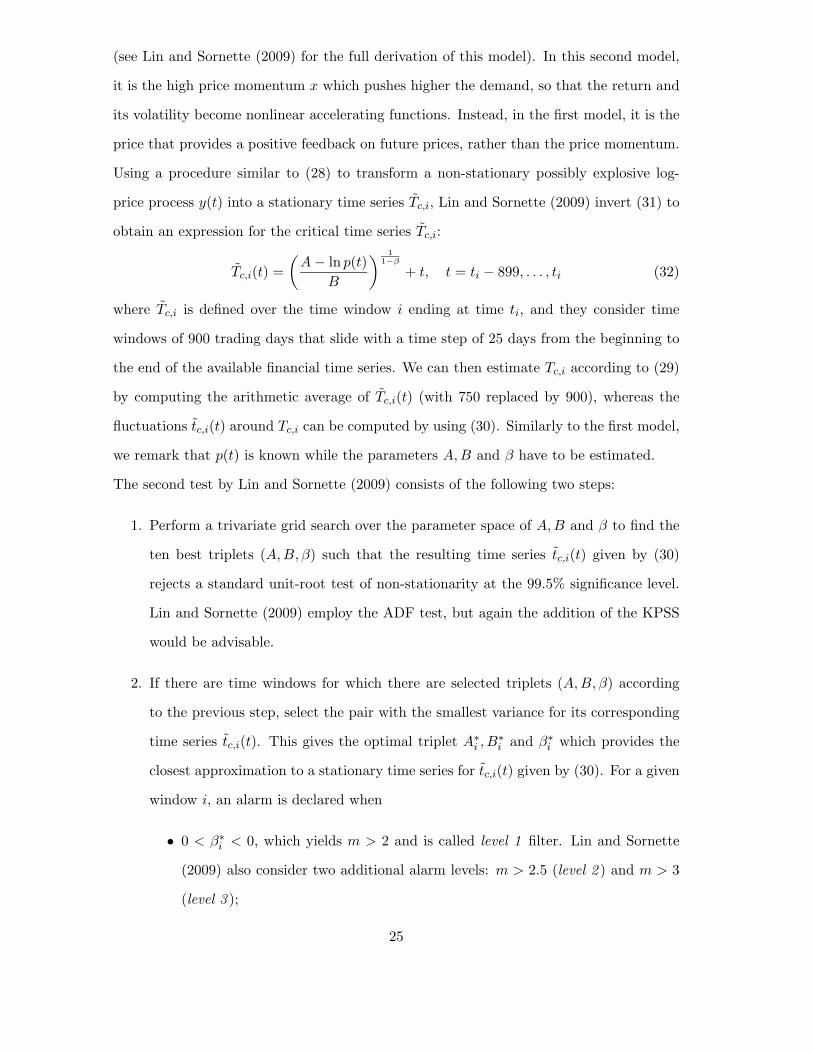
5.3 Graphical tools: The Crash Lock-In Plot (CLIP)

Fantazzini (2010a) proposed a graphical tool that proved to be useful to track the devel-

opment of a bubble and to understand whether a possible crash is in sight, or at least a

bubble deflation. The idea is to plot on the horizontal axis the date of the last observation

in the estimation sample, while on the vertical axis the estimated crash date tc computed

by fitting the LPPL to the data: if a change in the stock market regime is approaching,

then the recursively estimated tc should stabilize around a constant value close to the

critical time. Fantazzini (2010a) called such a plot the Crash Lock-In Plot (CLIP).

This idea can be easily justified theoretically by resorting to the models proposed by Lin

and Sornette (2009), in which the critical time Tc follows an Ornstein-Uhlenbeck process.

We report in Figure 2 the CLIPs for the Chinese Shanghai Composite Index in July 2009,

a case which was analyzed in details in Bastiaensen et al. (2009) and Jiang et al. (2010),

and for the SP500 in July 2007, being that the peak of the market in the decade. We used

data spanning from the global minima till 1 day before the market peak.

6 An Application: The Burst of the Gold Bubble in Decem-

ber 2009

The gold market peaked on the 02/12/2009, hitting the record high at $1,216.75 an ounce

in Europe, and then started falling on the 04/12/2009, losing more than 10% in two

weeks. The main concerns cited to be behind this bubble were the future prospects for

26

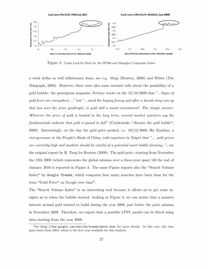
Figure 2: Crash Lock-In Plots for the SP500 and Shanghai Composite Index

a week dollar as well inflationary fears, see e.g. Mogi (Reuters, 2009) and White (The

Telegraph, 2009). However, there were also some worried calls about the possibility of a

gold bubble: the prestigious magazine Fortune wrote on the 12/10/2009 that ”...Signs of

gold fever are everywhere ...” but ”...amid the buying frenzy and after a decade-long run-up

that has seen the price quadruple, is gold still a smart investment? The simple answer:

Wherever the price of gold is headed in the long term, several market watchers say the

fundamentals indicate that gold is poised to fall” (Cendrowski, "Beware the gold bubble",

2009). Interestingly, on the day the gold price peaked, i.e. 02/12/2009, Hu Xiaolian, a

vice-governor at the People’s Bank of China, told reporters in Taipei that ”... gold prices

are currently high and markets should be careful of a potential asset bubble forming...”, see

the original report by R. Tung for Reuters (2009). The gold price, starting from November

the 12th 2008 (which represents the global minima over a three-year span) till the end of

January 2010 is reported in Figure 3. The same Figure reports also the "Search Volume

Index" by Google Trends, which computes how many searches have been done for the

term "Gold Price" on Google over time3.

The "Search Volume Index" is an interesting tool because it allows us to get some in-

sights as to when the bubble started: looking at Figure 3, we can notice that a massive

interest around gold started to build during the year 2008, just before the price minima

in November 2008. Therefore, we expect that a possible LPPL model can be fitted using

data starting from the year 2008.

3See http://www.google.com/intl/en/trends/about.html for more details. In this case, the timespan starts from 2004, which is the first year available for this analysis.

27

Figure 3: Gold price and Google Search Volume Index. Time t converted in units of 1-year

6.1 LPPL Fitting With Varying Window Sizes

Jiang et al. (2010) tested the stability of LPPL estimation parameters by varying the size

of the estimation samples and adopting the strategy of fixing one endpoint and varying the

other one, see also Sornette and Johansen (2001). By sampling many intervals as well as by

using bootstrap techniques, they obtained probabilistic predictions on the time intervals in

which a given bubble may end and lead to a new market regime (which may not necessarily

be a crash, but also a transition to a plateau or a slower decay). Following their example,

we fit the logarithm of the gold price by using the LPPL eq. (22) in shrinking windows

and in expanding windows. The shrinking windows have a fixed end date t2 = 01/12/2009,

while the starting date t1 increases from 12/11/2008 to 17/08/2009 in steps of five (trading)

days. The expanding windows have a fixed starting date t1 = 12/11/2008 while the end

date t2 increases from 17/08/2009 to 01/12/2009 in steps of five (trading) days.

Given the stochastic nature of the initial parameter selection and the noisy nature of the

underlying generating processes, we employed four estimation algorithms: the original

Taboo Search algorithm proposed by Cvijovic and Klinowski (1995), the 2-step nonlinear

optimization by Johansen et al. (2000), the Pure Random Search (PRS) and the 3-step

ML approach by Fantazzini (2010a)4. The estimation results are then filtered by the

4Similarly to Cvijovic and Klinowski (1995), we found that GA has a performance in between TabooSearch and PRS. However, even though PRS is computationally inefficient, it has the benefit to potentiallyvisit regions of the parameter space that sometimes are not visited by the previous algorithms. This is

28

following LPPL conditions, which were also used in Jiang et al. (2010) for the case of

Chinese bubbles: tc > t2, B < 0 and 0 < β < 1. The selected tc are then used to compute

the 20%/80% and 5%/95% quantile range of values of the crash dates which are reported

in Figure 4: the left plot shows the ranges which are obtained by considering the filtered

results from all four estimation methods, whereas the right plot shows the ranges obtained

by considering only the 2-step nonlinear optimization and the 3-step ML approach.

As expected, the original Taboo Search and the PRS are very inefficient methods compared

to the competing 2-step and 3-step approaches and deliver very large quantile ranges.

Nevertheless, the two medians tc, equal to 11/12/2009 for the left plot and 05/12/2009

for the right plot, are very close to the actual market peak date which occurred on the

02/12/2009 (i.e. 9.9206 when converted in units of one year). Moreover, if we consider

only the most efficient methods, the 20%/80% quantile interval is rather close and precise

and diagnoses that the critical time tc for the end of the bubble and the change of market

regime lies in the time sample 03/12/2009 - 11/12/2009 (the market started to fall on the

04/12/2009).

Figure 4: Quantile ranges of the crash date.

why we consider it in our analysis in the place of GA.

29

6.2 Diagnostic Tests based on the LPPL fitting residuals

We have discussed in section 3.2 that Lin et al. (2009) proposed a model for financial

bubbles where the LPPL fitting residuals follows a mean-reverting Ornstein-Uhlenbeck

process. Therefore, the corresponding residuals should follow a stationary AR(1) process

and this hypothesis can be tested by using unit root tests. We employed ADF and KPSS

tests: a rejection of the null hypothesis in the first test together with a failure to reject

the null in the second test, indicates that the residuals are stationary and thus compatible

with an O-U process.

We used the residuals resulting from the previous estimation windows and numerical al-

gorithms, that is 48 shrinking windows, 19 expanding windows and 4 estimation methods,

which gives a total of 268 calibrations. The fraction PLPPL of these different windows that

met the LPPL conditions was equal to PLPPL = 60.1%. The conditional probability that,

out of the fraction PLPPL of windows that satisfied the LPPL conditions, the null hypoth-

esis of non-stationarity was rejected for the residuals, was equal to PStat.Res.|LPPL = 100%

when using the ADF test at the probability level α = 0.001. As for the KPSS test, the

null of stationarity was not rejected at the 10% level or higher in all cases which satisfied

the LPPL conditions. Therefore, this empirical evidence is comparable with the results

reported by Jiang et al. (2010) for the case of the 2005-2007 and 2008-2009 Chinese stock

market bubbles.

6.3 Diagnostic Tests based on Rational Expectation Models with Stochas-

tic Mean-Reverting Termination Times

We employed the two diagnostics proposed by Lin and Sornette (2009) to detect the

presence of a bubble (and reviewed in Section 5.2) to the gold price time series, from

November the 12th 2008 to December the 1st 2009. As previously discussed, we considered

both the ADF and KPSS unit root tests. Moreover, we also used time windows of 500 and

250 trading days to compute the critical time series Tc,i in (28)-(29) and (32), together

with the original 750 trading days for the first diagnostic and 900 for the second one. The

rationale of this choice is that a long time span may include data which are not observed

during a bubble regime but during a standard Geometric Brownian Motion regime (or

30

other regimes). Of course, reducing the time window implies a loss of efficiency.

Interestingly the first procedure did not flag any alarm for the presence of a bubble,

whereas the second one flagged three series of alarms close to three important price falls,

see Figure 5: the first group of alarms was centered around the local market peak on the

20/02/2009 when gold reached the value of $995.3 an ounce, very close to the important

psychological barrier of $1000, and after two days it started falling, losing more than 10%

in two weeks. The second group of alarms was centered around the local market peak on

the 02/06/2009 when gold reached the value of $982.9 and after two days it started falling,

losing more than 5% in a week. Finally, the third group of alarms was centered around

the global market peak on the 02/12/2009 when gold reached the value of $1216 an ounce.

Figure 5: Logarithm of the gold price and corresponding alarms as vertical lines indicating the ends ofthe windows of T trading days, in which the second diagnostic flags an alarm for the presence of a bubble.The value of the exponent m for each alarm is reported in the legend .

This empirical evidence seems to suggest that the KPSS test provides more precise alarms

than the ADF test, which is not a surprise given the well known limitations of the latter

test. Moreover, a time window of 250 observations delivers more reliable flags for the

presence of a bubble (or imminent price falls) than longer time spans, being more robust

31

to market regime changes. However, a time window of 900 observations still provides

useful information.

6.4 Crash Lock-In Plots (CLIPs) for the Gold Bubble

The CLIP plots on the horizontal axis the date of the last observation in the estimation

sample, while on the vertical axis the estimated crash date tc computed by fitting the LPPL

to the data. Following the previous empirical evidence as well as the one reported in Lin

and Sornette (2009) and Fantazzini (2010a), we computed the CLIP by fitting the data

with two rolling estimation windows of 900 and 250 days, and by using the simple average

of the estimated tc resulting from the four estimation algorithms discussed in Section 6.1.

We used data spanning from the 12/11/2008 till 1 day before the global market peak on

the 02/12/2009. The two CLIPs are reported in Figure 6.

Figure 6: Crash Lock-In Plots for the Gold price series. The three vertical lines correspond to thetwo local market peaks on the 20/02/2009 and the 02/06/2009, and to the global market peak on the02/12/2009, respectively.

Not surprisingly, the indications provided by the two CLIPs are rather similar to those

provided by the second diagnostic test by Lin and Sornette (2009) discussed in the previous

section: the recursive forecasted crash dates computed with time windows of 250 trading

days stabilize around three constant values which are very close to the dates corresponding

to the two local market peaks on the 20/02/2009 and the 02/06/2009, and to the global

market peak on the 02/12/2009. The indications from the second CLIP computed with

time windows of 900 trading days are somewhat weaker, but confirm the previous alarms.

As expected, the estimates computed with smaller time spans are more noisy than those

32

with longer time spans.

7 Conclusions

We presented an easy-to-use and self-contained guide for modelling and detecting financial

bubbles with Log Periodic Power Laws, which contains the sufficient steps to derive the

main models and discusses the important aspects for practitioners and researchers. We

reviewed the original JLS model and we discussed early criticism to this approach and

recent generalizations proposed to answer these remarks. Moreover, we described three

different estimation methodologies which can be employed to estimate LPPLs models. We

then examined the issue of diagnosing bubbles in the making by using a set of different

techniques, that is by considering diagnostic tests based on the LPPL fitting residuals,

diagnostic tests based on rational expectation models with stochastic mean-reverting ter-

mination times, as well as graphical tools useful for capturing bubble development and for

understanding whether a crash is in sight or not. We finally presented a detailed empirical

application devoted to the burst of the gold bubble in December 2009, which highlighted

how a series of different diagnostics flagged an alarm for the presence of a bubble before

prices started to fall.

References[1] Abreu, D., and M. K., Brunnermeier. 2003. Bubbles and crashes. Econometrica, 71, no. 1: 173204.

[2] Bastiaensen, K., Cauwels, P., Sornette, D., Woodard, R., and W.X. Zhou. 2009. The Chinese equity bubble: Ready to burst.http://arxiv.org/abs/0907.1827.

[3] Bauwens, L., Lubrano, M., and J.F. Richard. 2000. Bayesian Inference In Dynamic Econometric Models. New York: OUP.

[4] Bernardo, J.M. and A.F.M. Smith. 1994. Bayesian Theory. New York: Wiley.

[5] Blanchard, O. J. 1979. Speculative bubbles, crashes and rational ex- pectations. Economics Letters, 3:387-389.

[6] Cendrowski, S. 2009. Beware the gold bubble. http://money.cnn.com/2009/10/06/pf/gold investing bubble.fortune/index.htm .

[7] Chang , G. and J. Feigenbaum. 2006. A Bayesian analysis of log-periodic precursors to financial crashes, Quantitative Finance6 (1), 15-36.

[8] Cvijovic, D. and J. Klinowski. (1995). Taboo search An approach to the multiple minima problem. Science, 267, no. 5: 664-666.

[9] Dennis, Jr., J.E., and R.B., Schnabel. 1983. Numerical Methods for Unconstrained Optimization and Nonlinear Equations. Engle-wood Cliffs: Prentice-Hall.

[10] Derrida, B., De Seze, L., and Itzykson, C. 1983. Fractal structure of zeros in hierarchical models. Journal of Statistical Physics,33: 559-569

[11] Fantazzini, D. 2010a. Modelling Bubbles And Anti-Bubbles In Bear Markets: A Medium-Term Trading Analysis. In Handbook ofTrading, ed. G. Gregoriou, 365-388. New York: McGraw-Hill.

[12] Fantazzini, D. 2010b. Modelling and Forecasting the Global Financial Crisis: Initial Findings using Heterosckedastic Log-PeriodicModels. Economics Bulletin, 30, no. 3: 1833-1841.

[13] Gazola,L., Fernandes, C., Pizzinga, A., and R. Riera. 2008. The log-periodic-AR(1)-GARCH(1,1) model for financial crashes,The European Physical Journal B, 61: 355-362.

33

[14] Goldenfeld, N. 1992. Lectures on phase transitions and the renormalization group. Reading: Addison-Wesley Publishing Company.

[15] Griffiths, W.E., Hill, R., and G.C. Lim. (2008). Using EViews for Principles of Econometrics. 3rd Edition, Hoboken, NJ: Wiley.

[16] Gulsten, M., Smith, E. A. and D.M. Tate. 1995. A Genetic Algorithm Approach to Curve Fitting. International Journal ofProduction Research, 33, no. 7: 1911-1923.

[17] Gurkaynak, R. 2008. Econometric tests of asset price bubbles: taking stock. Journal of Economic Surveys, 22, 1:166186.

[18] Hayashi, F. 2000. Econometrics. Princeton: PUP.

[19] Jacobsson, E. 2009. How to predict crashes in financial markets with the Log-Periodic Power Law. Master diss., Department ofMathematical Statistics, Stockholm University.

[20] Jiang, Z.Q., Zhou, W.H., Sornette, D., Woodard, R., Bastiaensen, K., and P. Cauwels. 2009. Bubble Diagnosis and Prediction ofthe 2005-2007 and 2008-2009 Chinese stock market bubbles (2009). Journal of Economic Behavior and Organization 74, 149-162(2010). Available at http://arxiv.org/abs/0909.1007

[21] Johansen, A. 2002. Comment on “Are financial crashes predictable?”, Europhysics Letters, 60, no. 5: 809-810.

[22] Johansen, A. 2003. Characterization of large price variations in financial markets. Physica A, 324: 157-166.

[23] Johansen, A., and D., Sornette. 1999. Financial anti-bubbles: Log-periodicity in Gold and Nikkei collapses. International Journalof Modern Physics C, 10, no. 4: 563-575.

[24] Johansen, A., and D., Sornette. 2000. Evaluation of the quantitative prediction of a trend reversal on the Japanese stock marketin 1999. International Journal of Modern Physics C, 11, no. 2: 359-364.

[25] Johansen, A., and D., Sornette. 2004. Endogenous versus Exogenous Crashes in Financial Markets, in Contemporary Issuesin International Finance, Nova Science Publishers. Reprinted as ’Shocks, Crashes and Bubbles in Financial Markets’, BrusselsEconomic Review (Cahiers economiques de Bruxelles), 49 (3/4), Special Issue on Nonlinear Analysis, 2006.

[26] Johansen, A., Ledoit, O. and D., Sornette. 2000. Crashes as critical points, International Journal of Theoretical and AppliedFinance, 3, no. 2: 219-255.

[27] Kaizoji, T., and D. Sornette., Market Bubbles and Crashes, in press in the Encyclopedia of Quantitative Finance (Wiley)http://www.wiley.com//legacy/wileychi/eqf/ (long version available at http://arXiv.org/abs/0812.2449)

[28] Koop, G. 2003. Bayesian Econometrics. Chichester: Wiley.

[29] Krugman, P. 1998. The Confidence Game, How Washington worsened Asia’s crash. The New Republic, October 5.

[30] Kwiatkowski, D., Phillips, P., Schmidt, P., and Y., Shin. 1992. Testing the null hypothesis of stationary against the alternativeof a unit root. Journal of Econometrics, 54: 159-178.

[31] Laloux, L., Potters, M., Cont,R., Aguilar, J.P and J.P. Bouchaud. 1999. Are financial crashes predictable?, Europhysics Letters,45, no. 1: 1-5.

[32] Landau, L.D. and E.M. Lifshitz. (1980). Statistical Physics, Part 1 and Part 2. 3rd ediion, Butterworth-Heinemann.

[33] Lin, L. and D. Sornette. 2009. Diagnostics of Rational Expectation Financial Bubbles with Stochastic Mean-Reverting Termi-nation Times. ETH working paper, http://arxiv.org/abs/0911.1921 .

[34] Lin, L., Ren., R.E. and D. Sornette. 2009. A Consistent Model of Explosive Financial Bubbles With Mean-Reversing Residuals,Quantitative Finance, in press. Available at http://arxiv.org/abs/0905.0128 and http://papers.ssrn.com/abstract=1407574.

[35] Mogi, C. 2009. Gold hits record high as dollar sets new lows. Reuters, November 26 2009,http://www.reuters.com/article/goldMktRpt/idUSSP7486520091126

[36] Ng, S. and P. Perron. 2001. Lag Length Selection and the Construction of Unit Root Tests with Good Size and Power. Econo-metrica, 69, no. 6: 1519-1554.

[37] Onsager, L. 1944. Crystal statistics. A two-dimensional model with an order-disorder transition. Physics Review, 65: 117-149.

[38] Pfaff, B. (2008). Analysis of Integrated and Cointegrated Time Series with R. New York: Wiley.

[39] Reinhart, C. and K. Rogoff. 2009. This Time is Different: Eight Centuries of Financial Folly. Princeton: PUP.

[40] Shefrin. H. 2005. A Behavioral Approach to Asset Pricing. Academic Press Advanced Finance Series. Burlington: Academic Press.

[41] Sornette, D. 2003a. Why Stock Markets Crash (Critical Events in Complex Financial Systems), Princeton: PUP.

[42] Sornette, D. 2003b. Critical market crashes. Physics Reports, 378, no. 1: 1-98.

[43] Sornette, D. 2009. Dragon-Kings, Black Swans and the Prediction of Crises, International Journal of Terraspace Science andEngineering, 2, no. 1: 1-18.

[44] Sornette, D. and A., Johansen. 1997. Large financial crashes, Physica A, 245: 411-422.

[45] Sornette, D. and A., Johansen. 2001. Significance of log-periodic precursors to financial crashes, Quantitative Finance, 1, no. 4:452-471.

34

[46] Sornette, D., and R. Woodard. 2010. Financial Bubbles, Real Estate bubbles, Derivative Bubbles, and the Financial and EconomicCrisis, in “Proceedings of APFA7 (Applications of Physics in Financial Analysis)”, New Approaches to the Analysis of Large-Scale Business and Economic Data, Misako Takayasu, Tsutomu Watanabe and Hideki Takayasu, eds., Springer. Available athttp://www.thic-apfa7.com/en/htm/index.html , http://arxiv.org/abs/0905.0220, http://web.sg.ethz.ch/wps/CCSS-09-00003/,and http://papers.ssrn.com/sol3/papers.cfm?abstract id=1407608

[47] Sornette, D. and W.X. Zhou. 2006. Predictability of Large Future Changes in major financial indices. International Journal ofForecasting, 22: 153-168.

[48] Sornette, D., Johansen, A. and J.P., Bouchaud. 1996. Stock market crashes, Precursors and Replicas, Journal de Physique I, 6:167-175.

[49] Sornette, D., Woodard, R. and W.X. Zhou. 2008. The 2006-2008 Oil Bubble and Beyond. ETH Zurich preprint.http://arXiv.org/abs/0806.1170

[50] Sornette, D., Woodard, R. and W.X. Zhou. 2009. The 2006-2008 Oil Bubble: Evidence of Speculation, and Prediction. PhysicaA, 388: 1571-1576.

[51] Stanley, H. E. 1971. Introduction to Phase Transitions and Critical Phenomena. New York: OUP.

[52] Stock J.H. 1994. Unit roots, structural breaks and trends. In Handbook of econometrics, ed. R.F. Engle, D.L. McFadden, vol. 4,ch. 47. Elsevier.

[53] Stock J.H., and M.W. Watson. (2002). Introduction to Econometrics. Addison Wesley.

[54] Tsay, R. 2005. Analysis of Financial Time Series. Chicago: Wiley.

[55] Tung, R. 2009. China c.Bank: Gold Prices High, Warns of Bubble. Reuters, December 02 2009,http://www.reuters.com/article/idUSTPU00193020091202 .

[56] White, G. 2009. Golden times for precious metals but pick carefully. The Telegraph, September 08 2009,http://www.telegraph.co.uk/finance/markets/questor/6156983/Golden-times-for-precious-metals-but-pick-carefully.html .

[57] Zhou, W.X., and D., Sornette. 2003. 2000-2003 Real Estate Bubble in the UK but not in the USA. Physica A, 329: 249-263.

[58] Zhou, W.X., and D., Sornette. 2005. Testing the Stability of the 2000-2003 US Stock Market Antibubble. Physica A, 348: 428-452.

[59] Zhou, W.X., and D., Sornette. 2006. Is There a Real-Estate Bubble in the US?. Physica A, 361: 297-308.

[60] Zhou, W.X., and D., Sornette. 2008. Analysis of the real estate market in Las Vegas: Bubble, seasonal patterns, and predictionof the CSW indexes. Physica A, 387: 243-260.

[61] Zhou, W.X., and D., Sornette. 2009. A case study of speculative financial bubbles in the South African stock market 2003-2006.Physica A, 388: 869-880.

35