Everyday predictions 1 Running head: EVERYDAY …web.mit.edu/cocosci/Papers/prediction10.pdf · A...

Everyday predictions 1

Running head: EVERYDAY PREDICTIONS

Optimal predictions in everyday cognition

Thomas L. Griffiths

Department of Cognitive and Linguistic Sciences

Brown University

Joshua B. Tenenbaum

Department of Brain and Cognitive Sciences

Massachusetts Institute of Technology

Word count: 3870

Address for correspondence:

Thomas Griffiths

Department of Cognitive and Linguistic Sciences

Brown University, Box 1978

Providence, RI 02912

Phone: (401) 863 9563 E-mail: tom [email protected]


Abstract

Human perception and memory are often explained as optimal statistical inferences,

informed by accurate prior probabilities. In contrast, cognitive judgments are usually

viewed as following error-prone heuristics, insensitive to priors. We examined the

optimality of human cognition in a more realistic context than typical laboratory studies,

asking people to make predictions about the duration or extent of everyday phenomena

such as human life spans and the box-office take of movies. Our results suggest that

everyday cognitive judgments follow the same optimal statistical principles as perception

and memory, and reveal a close correspondence between people’s implicit probabilistic

models and the statistics of the world.


Optimal predictions in everyday cognition

If you were assessing the prospects of a 60-year-old man, how much longer would

you expect him to live? If you were an executive evaluating the performance of a movie

that had made 40 million dollars at the box office so far, what would you estimate for its

total gross? Everyday life routinely poses such challenges of prediction, where the true

answer cannot be determined based on the limited data available, yet common sense

suggests at least a reasonable guess. Analogous inductive problems arise in many domains

of human psychology, such as identifying the three-dimensional structure underlying a

two-dimensional image (Freeman, 1994; Knill & Richards, 1996), or judging when a

particular fact is likely to be needed in the future (Anderson, 1990; Anderson & Milson,

1989). Accounts of human perception and memory suggest that these systems effectively

approximate optimal statistical inference, correctly combining new data with an accurate

probabilistic model of the environment (Anderson, 1990; Anderson & Milson, 1989;

Anderson & Schooler, 1991; Freeman, 1994; Geisler, Perry, Super, & Gallogly, 2001;

Huber, Shiffrin, Lyle, & Ruys, 2001; Knill & Richards, 1996; Kording & Wolpert, 2004;

Shiffrin & Steyvers, 1997; Simoncelli & Olshausen, 2001; Weiss, Simoncelli, & Adelson,

2002). In contrast – perhaps as a result of the great attention garnered by the work of

Kahneman, Tversky, and their colleagues (Kahneman, Slovic, & Tversky, 1982; Tversky &

Kahneman, 1974) – cognitive judgments under uncertainty are often characterized as the

result of error-prone heuristics, insensitive to prior probabilities. This view of cognition,

based on laboratory studies, appears starkly at odds with the near-optimality of other

human capacities, and with people’s ability to make smart predictions from sparse data in

the real world.

To evaluate how cognitive judgments compare with optimal statistical inferences in

real-world settings, we asked people to predict the duration or extent of everyday


phenomena such as human life spans and the gross of movies. We varied the phenomena

that were described and the amount of data available, and we compared the predictions of

human participants with those of an optimal Bayesian model, described in detail in the

Appendix. To illustrate the principles behind this Bayesian analysis, imagine that we

want to predict the total life span of a man we have just met, based upon the man’s

current age. If ttotal indicates the total amount of time the man will live and t indicates

his current age, the task is to estimate ttotal from t. The Bayesian predictor computes a

probability distribution over ttotal given t, by applying Bayes’ rule:

p(ttotal|t) ∝ p(t|ttotal)p(ttotal). (1)

The probability assigned to a particular value of ttotal is proportional to the product of

two factors: the likelihood p(t|ttotal) and the prior probability p(ttotal).

The likelihood is the probability of first encountering a person at age t given that

their total life span is ttotal. Assuming for simplicity that we are equally likely to meet a

person at any point in his life, this probability is uniform, p(t|ttotal) = 1/ttotal, for all

possible values of t between 0 and ttotal (and 0 for values outside that range). This

assumption of uniform random sampling is analogous to the “Copernican anthropic

principle” in Bayesian cosmology (Buch, 1994; Caves, 2000; Garrett & Coles, 1993; Gott,

1993, 1994; Ledford, Marriott, & Crowder, 2001) and the “generic view principle” in

Bayesian models of visual perception (Freeman, 1994; Knill & Richards, 1996). The prior

probability p(ttotal) reflects our general expectations about the relevant class of events – in

this case, about how likely it is that a person’s life span will be ttotal. Analysis of actuarial

data shows that the distribution of life spans in our society is (ignoring infant mortality)

approximately Gaussian – normally distributed – with a mean, µ, of about 75 years and a

standard deviation, σ, of about 16 years.

Combining the prior with the likelihood according to Equation 1 yields a probability


distribution p(ttotal|t) over all possible total life spans ttotal for a man encountered at age

t. A good guess for ttotal is the median of this distribution – that is, the point at which it

is equally likely that the true life span is longer or shorter. Taking the median of p(ttotal|t)

defines a Bayesian prediction function, specifying a predicted value of ttotal for each

observed value of t. Prediction functions for events with Gaussian priors are nonlinear: for

values of t much less than the mean of the prior, the predicted value of ttotal is

approximately the mean; once t approaches the mean, the predicted value of ttotal

increases slowly, converging to t as t increases but always remaining slightly higher, as

shown in Figure 1. Although its mathematical form is complex, this prediction function

makes intuitive sense for human life spans: a predicted life span of about 75 years would

be reasonable for a man encountered at age 18, 39, or 51; if we met a man at age 75 we

might be inclined to give him several more years at least; but if we met someone at age 96

we probably would not expect him to live much longer.

This approach to prediction is quite general, applicable to any problem that requires

estimating the upper limit of a duration, extent, or other numerical quantity given a

sample drawn from that interval (Buch, 1994; Caves, 2000; Garrett & Coles, 1993; Gott,

1993, 1994; Jaynes, 2003; Jeffreys, 1961; Ledford et al., 2001; Leslie, 1996; Maddox, 1994;

Shepard, 1987; Tenenbaum & Griffiths, 2001). However, different priors will be

appropriate for different kinds of phenomena, and the prediction function will vary

substantially as a result. For example, imagine trying to predict the total box office gross

of a movie given its take so far. The total gross of movies follows a power-law distribution,

with p(ttotal) ∝ t−γtotal for some γ > 0.1 This distribution has a highly non-Gaussian shape

(see Figure 1), with most movies taking in only modest amounts but occasional

blockbusters making huge amounts of money. In the Appendix, we show that for

power-law priors, the Bayesian prediction function picks a value for ttotal that is a multiple

of the observed sample t. The exact multiple depends on the parameter γ. For the


particular power law that best fits the actual distribution of movie grosses, an optimal

Bayesian observer would estimate the total gross to be approximately 50% greater than

the current gross: if we observe a movie has made $40 million to date, we should guess a

total gross of around $60 million; if we had observed a current gross of only $6 million, we

should guess about $9 million for the total. While such “constant multiple” prediction

rules are optimal for event classes that follow power-law priors, they are clearly

inappropriate for predicting life spans or other kinds of events with Gaussian priors. For

instance, upon meeting a 10-year-old child and her 75-year-old grandfather, we would

never predict that she will live a total of 15 years (1.5 × 10) and he will live to be 112

(1.5 × 75). Other classes of priors, such as the exponential-tailed Erlang distribution,

p(ttotal) ∝ ttotal exp{−ttotal/β} for β > 0,2 are also associated with distinctive optimal

prediction functions. For the Erlang distribution, the best guess of ttotal is simply t plus a

constant determined by the parameter β, as shown in the Appendix and illustrated in

Figure 1.

Our experiment compared these ideal Bayesian analyses with the judgments of a

large sample of human participants, examining whether people’s predictions were sensitive

to the distributions of different quantities that arise in everyday contexts. We used

publicly available data to identify the true prior distributions for several classes of events

(the sources of these data are given in Table A1 in the Appendix). For example, as shown

in Figure 2, human life spans and the runtime of movies are approximately Gaussian, the

gross of movies and the length of poems are approximately power-law distributed, and the

number of years spent in office for members of the U.S. House of Representatives and the

reigns of Pharaohs are approximately Erlang. The experiment examined how well people’s

predictions corresponded to optimal statistical inference in these different settings.


Methods

Participants

Participants were tested in two groups, with each group making predictions about

five different phenomena. One group of 208 undergraduates made predictions about Movie

Grosses, Poems, Life Spans, Pharaohs, and Marriages. A second group of 142

undergraduates made predictions about Movie Runtimes, Representatives, Cakes, Waiting

Times, and Marriages.

Materials

Within each group, each participant made predictions about one phenomenon from

each of the five different classes seen by that group. Predictions were based on one of five

possible values of t, varied randomly between subjects. These values were: 1, 6, 10, 40,

and 100 million dollars for Movie Grosses: 2, 5, 12, 32, and 67 lines for Poems; 18, 39, 61,

83, and 96 years for Life Spans; 1, 3, 7, 11, and 23 years for Pharaohs; 1, 3, 7, 11, and 23

years for Marriages; 30, 60, 80, 95, and 110 minutes for Movie Runtimes; 1, 3, 7, 15 and 31

years for Representatives; 10, 20, 35, 50 and 70 minutes for Cakes; and 1, 3, 7, 11, and 23

minutes for Waiting Times. In each case, participants read several sentences establishing

context and then were asked to predict ttotal given t.

The questions were presented in survey format. A paragraph began each survey as

follows:

Each of the questions below asks you to predict something – either a duration

or a quantity – based on a single piece of information. Please read each

question and write your prediction on the line below it. We’re interested in

your intuitions, so please don’t make complicated calculations – just tell us

what you think!


Each question was then introduced with a couple of sentences to provide a context.

Sample questions were:

Movie Grosses: Imagine you hear about a movie that has taken in 10 million

dollars at the box office, but don’t know how long it has been running. What

would you predict for the total amount that of box office intake for that movie?

Poems. If your friend read you her favourite line of poetry, and told you it was

line 5 of a poem, what would you predict for the total length of the poem?

Life Spans. Insurance agencies employ actuaries to make predictions about

people’s life spans – the age at which they will die – based upon demographic

information. If you were assessing an insurance case for an 18 year old man,

what would you predict for his life span?

Pharaohs. If you opened a book about the history of ancient Egypt to a page

listing the reigns of the pharaohs, and noticed that at 4000 BC a particular

pharaoh had been ruling for 11 years, what would you predict for the total

duration of his reign?

Marriages. A friend is telling you about an acquaintance whom you do not

know. In passing, he happens to mention that this person has been married for

23 years. How long do you think this person’s marriage will last?

Movie Runtimes. If you made a surprise visit to a friend, and found that they

had been watching a movie for 30 minutes, what would you predict for the

length of the movie?

Representatives. If you heard a member of the House of Representatives had

served for 15 years, what would you predict his total term in the House would

be?


Cakes. Imagine you are in somebody’s kitchen and notice that a cake is in the

oven. The timer shows that it has been baking for 35 minutes. What would

you predict for the total amount of time the cake needs to bake?

Waiting Times. If you were calling a telephone box office to book tickets and

had been on hold for 3 minutes, what would you predict for the total time you

would be on hold?

Procedure

Participants completed the surveys as part of a booklet of unrelated experiments.

Results

We first filtered out responses that could not be analyzed or indicated a

misunderstanding of the task, removing predictions which did not correspond to numerical

values or were less than ttotal. Only a small minority of responses failed to meet this

criterion for all stimuli except Marriages, yielding 174, 197, 197, 191, 136, 130, 126, and

158 for Movie Grosses, Poems, Life Spans, Pharaohs, Movie Runtimes, Representatives,

Cakes, and Waiting Times respectively. The responses for the Marriages stimulus were

problematic because the majority of participants (52%) indicated that marriages last

“forever”. This accurately reflects the proportion of marriages that end in divorce

(Kreider & Fields, 2002), but prevents the data from being analyzed using the methods

described below, which are based upon median values. We thus did not analyze responses

for the Marriages stimuli further.

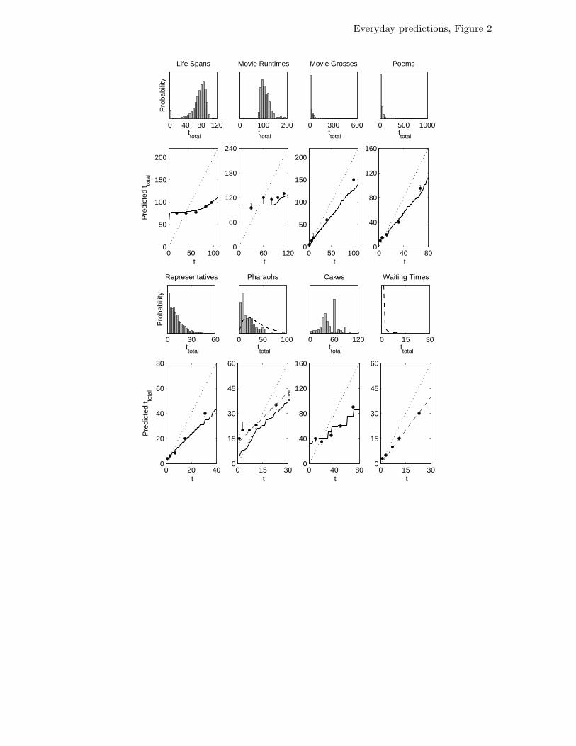
People’s judgments for Life Spans, Movie Runtimes, Movie Grosses, Poems, and

Representatives were indistinguishable from optimal Bayesian predictions based on the

empirical prior distributions, as shown in Figure 2. People’s prediction functions took on

very different shapes in domains characterized by Gaussian, power-law, or Erlang priors,


just as expected under the ideal Bayesian analysis. Notably, the model predictions shown

in Figure 2 have no free parameters tuned specifically to fit the human data, but are

simply the optimal functions prescribed by Bayesian inference given the relevant world

statistics. These results are inconsistent with claims that cognitive judgments are based

on non-Bayesian heuristics that are insensitive to priors (Kahneman et al., 1982; Tversky

& Kahneman, 1974). The results are also inconsistent with simpler Bayesian prediction

models that adopt a single uninformative prior, p(ttotal) ∝ 1/ttotal, regardless of the

phenomenon to be predicted (Gott, 1993, 1994; Jaynes, 2003; Jeffreys, 1961; Ledford

et al., 2001).

Examining the remaining stimuli – Pharaohs, Cakes, and Waiting Times – provides

the opportunity to learn about the limits of people’s capacity for prediction. As shown in

Figure 2, people’s predictions about the reigns of pharaohs had a form consistent with the

appropriate prior (an Erlang distribution), but were slightly too high. We established

people’s subjective priors for the reigns of pharaohs in a follow-up experiment, asking 35

undergraduates to state the typical duration of a pharaoh’s reign. The median response

was 30 years, which corresponds to an Erlang prior on ttotal with parameter β = 17.9, as

opposed to the true value of approximately β = 9.34. Using this subjective Erlang prior

produces a close correspondence to human judgments.

The results for the Pharaohs stimuli provide an instance of a situation in which

people make inaccurate predictions: when they know the appropriate form for the prior,

but not the details of its parameters. In contrast, responses to the Cakes stimuli reveal

that people can make accurate predictions even in contexts where priors lack a simple

form. These stimuli ask about the duration a cake should spend in the oven, a quantity

that follows a rather irregular distribution, as shown in Figure 2. However, people’s

judgments were still close to the ideal Bayesian predictions, despite the complex form of

the empirical prior distribution.


These results suggest that people’s predictions can also be used as a method for

identifying the prior beliefs that inform them. The Waiting Times stimuli provide the

opportunity to explore this possibility. The true distribution of waiting times in queues is

currently a controversial question in operations research. Traditional models, based on the

Poisson process, assume that waiting times follow a distribution with exponential tails

(e.g., Hillier & Lieberman, 2001). However, several recent analyses suggest that in many

cases, waiting times may be better approximated by a power-law distribution (Barabasi,

2005, provides a summary and explanation of these findings). Hence it is not so clear

what the objective distribution of durations should be for these stimuli. Rather than using

objective statistics on real-world durations to assess the optimality of people’s judgments,

as we did for the other stimulus classes, we used people’s judgments on these stimuli to

assess which distributional form they are assuming the phenomena will follow. We fit

prediction functions for Gaussian, power-law, and Erlang distributions to the behavioral

data, attempting to minimize the sum of the squared differences between the median

human judgments and the predicted values of ttotal. The power-law prior with γ = 2.43

provided the best fit to human judgments, producing the predictions shown in Figure 2.

Assuming that people’s predictions are near-optimal with respect to the true distribution

of durations, these results are qualitatively consistent with recent power-law models for

waiting time distributions (Barabasi, 2005).

Discussion

The results of our experiment reveal a far closer correspondence between optimal

statistical inference and everyday cognition than suggested by previous research. People’s

judgments were close to the optimal predictions produced by our Bayesian model across a

wide range of settings. These judgments also serve as a guide to people’s implicit beliefs

about the distributions of everyday quantities, and reveal that these beliefs are


surprisingly consistent with the statistics of the world. This finding parallels formal

analyses of perception and memory, in which accurate probabilistic models of the

environment play a key role in the solution of inductive problems (Anderson, 1990;

Anderson & Milson, 1989; Anderson & Schooler, 1991; Freeman, 1994; Geisler et al., 2001;

Huber et al., 2001; Knill & Richards, 1996; Kording & Wolpert, 2004; Shiffrin & Steyvers,

1997; Simoncelli & Olshausen, 2001; Weiss et al., 2002).

While people’s predictions about everyday events were on the whole extremely

accurate, the cases in which their predictions deviated from optimality may help to shed

light on the implicit assumptions and strategies that make these intuitive judgments so

successful most of the time in the real world. One interesting hypothesis of this sort is

suggested by the pattern of people’s errors in predicting the reigns of pharaohs. Both the

median judgment error and the variance in judgments across participants was substantially

greater for this task than for our other tasks. This should not be surprising, as most

participants probably had far less direct experience with the reigns of pharaohs than with

the other kinds of scenarios we presented. Despite this lack of direct experience, people’s

predictions were not completely off the mark: their judgments were consistent with having

implicit knowledge of the correct form of the underlying distribution but making incorrect

assumptions about how this form should be parameterized (i.e., its mean value).

The predictions for the Pharaohs stimuli suggest a general strategy people might

employ to make predictions about unfamiliar kinds of events, which is surely an important

version of the prediction problem as it arises in everyday life. Given an unfamiliar task,

people might be able to identify the appropriate form of the distribution by making an

analogy to more familiar phenomena in the same broad class, even if they do not have

sufficient direct experience to set the parameters of that distribution accurately. For

instance, participants might have been familiar with the times that various modern

monarchs spend in their positions, as well as with the causal mechanisms (e.g., succession,


death) responsible for those times, and it is not unreasonable to think that analogous

mechanisms could have governed the durations of Pharaohs’ reigns in ancient Egypt. Yet

most people might not be aware of (or might not remember) just how short lifespans

typically were in ancient Egypt compared to our modern expectations, even if they know

they were somewhat shorter. If participants made predictions on the Pharaohs task by

drawing an analogy to modern monarchs and adjusting the mean reign duration

downwards by some uncertain but insufficient factor, that would be entirely consistent

with the pattern of errors we observed. Such a strategy of prediction-by-analogy could be

an adaptive way of making judgments that would otherwise lie beyond people’s limited

base of knowledge and experience.

The finding of optimal statistical inference in an important class of cognitive

judgments resonates with a number of recent suggestions that Bayesian statistics may

provide a general framework for analyzing human inductive inferences. Bayesian models

require making the assumptions of a learner explicit. By exploring the implications of

different assumptions, it becomes possible to explain many of the interesting and

apparently inexplicable aspects of human reasoning (e.g., McKenzie, 2003). The ability to

combine accurate background knowledge about the world with rational statistical

updating is critical in many aspects of higher-level cognition. Bayesian models have been

proposed for learning words and concepts (Tenenbaum, 1999), forming generalizations

about the properties of objects (Shepard, 1987; Tenenbaum & Griffiths, 2001; Anderson,

1990) and discovering logical or causal relations (Anderson, 1990; Oaksford & Chater,

1994; Griffiths & Tenenbaum, in press). However, these modeling efforts have not

typically attempted to establish optimality in real-world environments. Our results

demonstrate that, at least for a range of everyday prediction tasks, people effectively

adopt prior distributions that are accurately calibrated to the statistics of relevant events

in the world. Assessing the scope and depth of the correspondence between probabilities


in the mind and those in the world presents a fundamental challenge for future work.


References

Anderson, J. R. (1990). The adaptive character of thought. Hillsdale, NJ: Erlbaum.

Anderson, J. R., & Milson, R. (1989). Human memory: An adaptive perspective.

Psychological Review, 96, 703-719.

Anderson, J. R., & Schooler, L. J. (1991). Reflections of the environment in memory.

Psychological Science, 2, 396-408.

Barabasi, A.-L. (2005). The origin of bursts and heavy tails in human dynamics. Nature,

435, 207-211.

Buch, P. (1994). Future prospects discussed. Nature, 368, 107-108.

Caves, C. M. (2000). Predicting future duration from present age: A critical assessment.

Contemporary Physics, 41, 143-153.

Freeman, W. T. (1994). The generic viewpoint assumption in a framework for visual

perception. Nature, 368, 542-545.

Garrett, A. J. M., & Coles, P. (1993). Bayesian inductive inference and the anthropic

principles. Comments on Astrophysics, 17, 23-47.

Geisler, W. S., Perry, J. S., Super, B. J., & Gallogly, D. P. (2001). Edge co-occurrence in

natural images predicts contour grouping performance. Vision Research, 41,

711-724.

Gott, J. R. (1993). Implications of the Copernican principle for our future prospects.

Nature, 363, 315-319.

Gott, J. R. (1994). Future prospects discussed. Nature, 368, 108.

Griffiths, T. L., & Tenenbaum, J. B. (in press). Elemental causal induction. Cognitive

Psychology.


Hillier, F. S., & Lieberman, G. J. (2001). Introduction to operations research (7 ed.). New

York: McGraw Hill.

Huber, D. E., Shiffrin, R. M., Lyle, K. B., & Ruys, K. I. (2001). Perception and

preference in short-term word priming. Psychological Review, 108, 149-182.

Jaynes, E. T. (2003). Probability theory: The logic of science. Cambridge: Cambridge

University Press.

Jeffreys, H. (1961). Theory of probability. Oxford: Oxford University Press.

Kahneman, D., Slovic, P., & Tversky, A. (Eds.). (1982). Judgment under uncertainty:

Heuristics and biases. Cambridge: Cambridge University Press.

Knill, D. C., & Richards, W. A. (1996). Perception as Bayesian inference. Cambridge:

Cambridge University Press.

Kording, K., & Wolpert, D. M. (2004). Bayesian integration in sensorimotor learning.

Nature, 427, 244-247.

Kreider, R. M., & Fields, J. M. (2002). Number, timing, and duration of marriages and

divorces: 1996. (U.S. Census Bureau Current Population Reports)

Ledford, A., Marriott, P., & Crowder, M. (2001). Lifetime prediction from only present

age: fact or fiction? Physics Letters A, 280, 309-311.

Leslie, J. (1996). The end of the world: The ethics and science of human extinction.

London: Routledge.

Maddox, J. (1994). Star masses and Bayesian probability. Nature, 371, 649.

McKenzie, C. R. M. (2003). Rational models as theories – not standards – of behavior.

Trends in Cognitive Sciences, 7, 403-406.

Oaksford, M., & Chater, N. (1994). A rational analysis of the selection task as optimal

data selection. Psychological Review, 101, 608-631.


Shepard, R. N. (1987). Towards a universal law of generalization for psychological science.

Science, 237, 1317-1323.

Shiffrin, R. M., & Steyvers, M. (1997). A model for recognition memory: REM:

Retrieving Effectively from Memory. Psychonomic Bulletin & Review, 4, 145-166.

Simoncelli, E. P., & Olshausen, B. (2001). Natural image statistics and neural

representation. Annual Review of Neuroscience, 24, 1193-1216.

Tenenbaum, J. B. (1999). Bayesian modeling of human concept learning. In M. S. Kearns,

S. A. Solla, & D. A. Cohn (Eds.), Advances in neural information processing

systems 11 (p. 59-65). Cambridge, MA: MIT Press.

Tenenbaum, J. B., & Griffiths, T. L. (2001). Generalization, similarity, and Bayesian

inference. Behavioral and Brain Sciences, 24, 629-641.

Tversky, A., & Kahneman, D. (1974). Judgment under uncertainty: heuristics and biases.

Science, 185, 1124-1131.

Weiss, Y., Simoncelli, E. P., & Adelson, E. H. (2002). Motion illusions as optimal

percepts. Nature Neuroscience, 5, 598-604.


Appendix

The prediction problem

Assume that a point t is sampled uniformly at random from the interval [0, ttotal).

What should we guess for the value of ttotal? A Bayesian solution to this problem involves

computing the posterior distribution over ttotal given t. Applying Bayes’ rule, this is

p(ttotal|t) =p(t|ttotal)p(ttotal)

p(t)(2)

where

p(t) =

∫

∞

0p(t|ttotal)p(ttotal) dttotal. (3)

By the assumption that t is sampled uniformly at random, p(t|ttotal) = 1/ttotal for

ttotal ≥ t and 0 otherwise. Equation 3 thus simplifies to

p(t) =

∫

∞

t

p(ttotal)

ttotaldttotal (4)

The form of the posterior distribution for any given value of t is thus determined entirely

by the prior, p(ttotal).

We can derive an analytic form for the posterior distribution obtained with

power-law and Erlang priors. The posterior distribution resulting from the Gaussian prior

has no simple analytic form. With the power-law prior, p(ttotal) ∝ t−γtotal for γ > 0. This

prior is improper if γ ≤ 1, since the integral over ttotal diverges, but the posterior remains

a proper probability distribution regardless. Applying Equation 4, we have

p(t) ∝

∫

∞

tt−(γ+1)total dttotal

= − 1γ t−γ

total

∣

∣

∣

∞

t

= 1γ t−γ ,

where the constant of proportionality remains the same as in the original prior. We can


substitute this result into Bayes’ rule (Equation 2) to obtain

p(ttotal|t) =t−(γ+1)total1γ t−γ

=γ tγ

tγ+1total

, (5)

for all values of ttotal ≥ t. Under the Erlang prior, p(ttotal) ∝ ttotal exp{−ttotal/β}, we have

p(t) ∝

∫

∞

texp{−ttotal/β}

= −β exp{−ttotal/β} |∞

t

= β exp{−t/β}

where the constant of proportionality remains the same as in the original prior. Again, we

can substitute this result into Bayes’ rule (Equation 2) to obtain

p(ttotal|t) =exp{−ttotal/β}

β exp{−t/β}

= 1β exp{−(ttotal − t)/β}, (6)

for all values of ttotal ≥ t.

Predicting ttotal

We take the predicted value of ttotal, which we will denote t∗, to be the posterior

median. This is the point t∗ such that P (ttotal > t∗|t) = 0.5: a Bayesian predictor believes

that there is a 50% chance that the true value of ttotal is greater than t∗, and a 50%

chance that the true value of ttotal is less than t∗. This point can be computed from the

posterior, using the fact that

P (ttotal > t∗|t) =

∫

∞

t∗p(ttotal|t) dttotal . (7)

We can derive t∗ analytically in the case of a power-law or Erlang prior. For the


power-law prior, we can use Equation 5 to rewrite Equation 7 as


∫

∞

t∗

γ tγ

tγ+1total

dttotal

= −

(

t

ttotal

)γ ∣

∣

∣

∣

∞

t∗

=

(

t

t∗

)γ

. (8)

We can now solve for t∗ such that P (ttotal > t∗|t) = 0.5, obtaining t∗ = 21/γt. For the

Erlang prior, we can use Equation 6 to rewrite Equation 7 as


∫

∞

t∗

1β exp{−(ttotal − t)/β}dttotal

= − exp{−(ttotal − t)/β}|∞t∗

= exp{−(t∗ − t)/β}. (9)

Again, we can solve for t∗ such that P (ttotal > t∗|t) = 0.5, obtaining t∗ = t + β log 2. For

the Gaussian prior, we can find values of t∗ by numerical integration and optimization.


Author Note

We thank Liz Baraff and Onny Chatterjee for their assistance in running the

experiments, and Mira Bernstein, Daniel Casasanto, Nick Chater, David Danks, Peter

Dayan, Reid Hastie, Konrad Kording, Tania Lombrozo, Rebecca Saxe, Marty Tenenbaum

and an anonymous reviewer for comments on the manuscript. The second author was

supported by the Paul E. Newton Chair.


Footnotes

1When γ > 1, a power-law distribution is often referred to in statistics and economics

as a Pareto distribution.

2The Erlang distribution is a special case of the Gamma distribution. The Gamma

distribution is p(ttotal) ∝ tk−1total exp{−ttotal/β}, where k > 0 is a real number. The Erlang

distribution assumes that k is an integer. Following Shepard (1987), we use a

one-parameter Erlang distribution, fixing k = 2.


Table A1: Sources of Data for Estimating Prior Distributions

Dataset Source (number of datapoints)

Move Grosses http://www.worldwideboxoffice.com/ (5302)

Poems http://www.emule.com (1000)

Life Spans http://www.demog.berkeley.edu/wilmoth/mortality/states.html (complete lifetable)

Movie Runtimes http://www.imdb.com/Charts/usboxarchive/ (233 top 10 movies from 1998-2003)

Representatives http://bioguide.congress.gov (2150 members since 1945)

Cakes http://www.allrecipes.com/ (619)

Pharaohs http://www.touregypt.net/ (126)


Figure Captions

Figure 1. Optimal Bayesian prediction functions depend on the form of the prior

distribution. Three columns represent qualitatively different statistical models appropriate

for different kinds of events. The top row of plots shows three parametric families of prior

distributions for the total duration or extent, ttotal, that could describe events in a

particular class. Lines of different styles represent different parameter values (e.g.,

different mean durations) within each family. The bottom row of plots shows the optimal

predictions for ttotal as a function of t, the observed duration or extent of an event so far,

assuming the prior distributions shown in the top panel. For Gaussian priors (column 1)

the prediction function always has slope less than one and an intercept near the mean µ:

predictions are never much smaller than the mean of the prior distribution, nor much

larger than the observed duration. Power-law priors (column 2) result in linear prediction

functions with variable slope and a zero intercept. Erlang priors (column 3) yield a linear

prediction function that always has slope equal to one and a nonzero intercept.

Figure 2. People’s predictions for various everyday phenomena. The top row of plots

shows the empirical distributions of the total duration or extent, ttotal, for each of these

phenomena. The first two distributions are approximately Gaussian, the third and fourth

are approximately power-law, and the fifth and sixth are approximately Erlang. The

bottom row shows predicted values of ttotal for a single observed sample t of a duration or

extent for each phenomenon. Black dots show median predictions of ttotal for human

participants. Error bars indicate 68% confidence intervals (estimated by a 1000-sample

bootstrap). Solid lines show the optimal Bayesian predictions based on the empirical prior

distributions shown above. Dashed lines show predictions made by estimating a subjective

prior, for the Pharaohs and Waiting Times stimuli, as explained in the main text. Dotted

lines show predictions based on a fixed uninformative prior (Gott, 1993).

Everyday predictions, Figure 1

0 50 100 t

total

Power−law prior

0 50 100 t

total

Erlang prior

0 50 100 t

total

Gaussian prior

Pro

babi

lity

0 15 300

15

30

45

60

t

γ=1γ=1.5γ=2

0 15 300

15

30

45

60

t

β=30β=18β=10

0 15 300

15

30

45

60

t

Pre

dict

ed t to

tal

µ=30µ=25µ=15

Everyday predictions, Figure 2

0 40 80 120 t

total

Life Spans

Pro

babi

lity

0 100 200

Movie Runtimes

ttotal

0 300 600 t

total

Movie Grosses

0 500 1000 t

total

Poems

0 50 1000

50

100

150

200

t

Pre

dict

ed t to

tal

0 60 1200

60

120

180

240

t0 50 100

0

50

100

150

200

t0 40 80

0

40

80

120

160

t

0 20 400

20

40

60

80

t

Pre

dict

ed t to

tal

0 40 800

40

80

120

160

t

Pre

dict

ed t to

tal

0 15 300

15

30

45

60

t0 15 30

0

15

30

45

60

t

0 30 60 t

total

Representatives

Pro

babi

lity

0 50 100 t

total

Pharaohs

0 60 120

Cakes

ttotal

0 15 30

Waiting Times

ttotal

Everyday predictions 1 Running head: EVERYDAY …web.mit.edu/cocosci/Papers/prediction10.pdf · A...

Documents

Transcript of Everyday predictions 1 Running head: EVERYDAY …web.mit.edu/cocosci/Papers/prediction10.pdf · A...