Evaluation of the Environmental Caucus's Binomial Method Critique

Steven G. Saiz Division of Water Quality

SWRCB

March 3.2004

Introduction

Craig Wilson asked me to evaluate comments sent to the Monitoring and TMDL Listing Unit in response to the recent release of the SWRCB Water Quality Control Policy for Developing California's Clean Water Act Section 303(d) List. Several environmental groups joined efforts and commented on the statistical decision-making errors expected when using the binomial statistical model proposed in the Policy.

My evaluation of the Environmental Caucus's critique reflects my personal observations and is my attempt to explain and expand upon the ideas presented by the Caucus.

Specifically, the Environmental Caucus has argued that the Policy's binomial model is biased in favor of not listing water bodies. Appendix I of the Environmental Caucus's comment document presented an expression to calculate the probability of failing to list a water body when the true exceedance rate is greater than 0.1. This probability is known as a beta statistical error, P. The Environmental Caucus presented the expression below (their equation Al) as an analytical solution to calculate p:

where N = sample size, klist =number of exceedances in N samples needed in order to list the water body with a significance level of 10% (i.e., with 90% confidence), and r = the true unknown exceedance rate.

Similarly, the Environmental Caucus presented an expression for the probability of incorrectly listing a clean water body when the true exceedance rate is 5 0.1. This is known as an alpha statistical error, a.The Environmental Caucus presented the expression below (their equation A4) as an analytical solution to calculate a:

Numeric solutions to these equations for various sample sizes were presented in Table 1of the Environmental Caucus document and are reproduced in Table 1 of this document.

Observations

Observation 1. The statistical probabilities presented in Table 1 are the sum of all possible statistical errors over all possible alternate exceedance rates.

The given values are an attempt to summarize a and j3 errors over a continuous range of alternate exceedance rates. The definite integral portion of both equations effectively sums up the total statistical error for infinitely small changes in alternate exceedance rates. The resulting Table 1 "a" values are therefore summations of all a s for 0 5 r 50.1 and should more properly be expressed symbolically as Ca. Similarly, the Table 1 "P" values are summations of all ps for 0.1 < r (1 and should more properly be expressed as CP. The units of these summations are (probability of error x alternate exceedance rate) and not probability of error, per se.

To help illustrate what the summations are measuring, I created a power curve graph (Fig 1) for a one-sided binomial hypothesis test with N=10. Values in this graph were calculated (Gibbons 1964) by finding the probability of rejecting the null hypothesis (Ho: r 5 0.1) under many alternate exceedance rates when the nominal significance level remains at lo%,

N

P(rejectHo) =P(k tklist ( r, N) = ( N! )rk(1-r)( N - k ) k.kiisr k!(n -k)!

The right side of this expression is the standard cumulative binomial probability distribution. When r 5 0.1 the above expression is an estimate of a. When r > 0.1 the above expression is an estimate of statistical power (1 - p), the probability of correctly rejecting a false null hypothesis.

Taking unity minus these probabilities produces a graph of the statistical confidence coefficient and p, respectively, (Fig. 2) over a range of alternate exceedance rates. Finally, both statistical errors, a and p, are shown in Figure 3 along with the summations, Ca and Cp, produced by the definite integrals in equations A4 and Al.

These summations are areas under the statistical error curves. We do not expect X a +CP to add to one, as is required by a probability density function. Rather we expect Ca + (0.1-Ca) + CP + (0.9 - Cp) to equal unity. The expressions in parentheses are the areas above the error curves in Figure 3.

An alternative approach to estimating the C a and CP values is through the use of Riemann sums (Ellis & Gulick 1994, p.293). For example, let f represent the beta error function in Figure 3. We may partition the interval [O. 1, 11 into n subdivisions of size Ar. The area under f is then approximated as,

where r k is any arbitrary alternate exceedance rate within the kth subdivision andf(rk) is the beta error associated with the altemate exceedance rate, rk. Increasing the number of subdivisions -will produce increasingly accurate estimates of CP (Table 3) and these approximations will converge on the Cp values given in Table 1. Again, note that the elements being summed in the above summation have units of @robability of error x altemate exceedance rate).

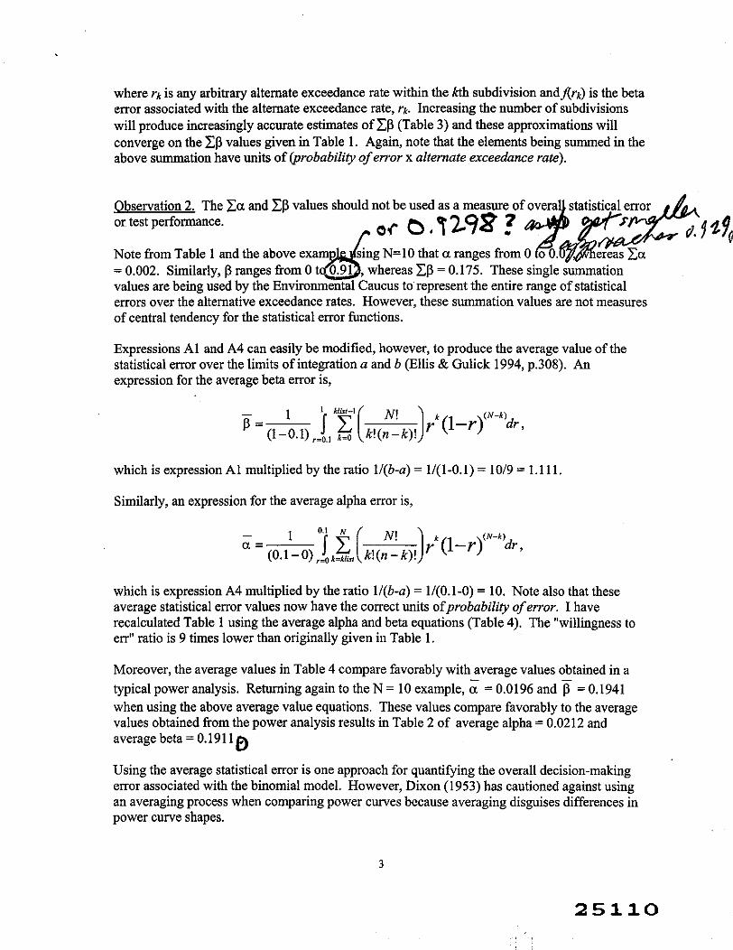
Observation 2. The xa and CP values should or test performance. . Note from Table 1 and the above exam = 0.002. Similarly, P ranges from 0 values are being used by the Environmental Caucus to represent the entire range of statistical errors over the alternative exceedance rates. However, these summation values are not measures of central tendency for the statistical error functions.

Expressions A1 and A4 can easily be modified, however, to produce the average value of the statistical error over the limits of integration a and b (Ellis & Gulick 1994, p.308). An expression for the average beta error is,

which is expression A1 multiplied by the ratio ll(b-a) = 141-0.1) = 1019= 1.1 11.

Similarly, an expression for the average alpha error is,

-a =

0 1-0 , O / t (

k!(nN! -k)!

( 1 - (N-k)dr,

which is expression A4 multiplied by the ratio ll(b-a) = ll(0.1-0) = 10. Note also that these average statistical error values now have the correct units ofprobability of error. I have recalculated Table 1 using the average alpha and beta equations (Table 4). The "willingness to err" ratio is 9 times lower than originally given in Table 1.

Moreover, the average values in Table 4 compare favorably with average values obtained in a typical power analysis. Returning again to the N = 10 example, = 0.0196 and p = 0.1941 when using the above average value equations. These values compare favorably to the average values obtained from the power analysis results in Table 2 of average alpha = 0.0212 and average beta = 0.191 1 0

Using the average statistical error is one approach for quantifying the overall decision-making error associated with the binomial model. However, Dixon (1953) has cautioned against using an averaging process when comparing power curves because averaging disguises differences in power curve shapes.

Observation 3. The "willingness to err" ratio is of theoretical importance only.

In practice, only one type of decision-making error can be made for a given tested water body. Ideally, we will make a correct decision. If we do make a decision error then it will be either an a error or a p error, never both. Therefore, to express the ratio of P to a may not make sense from a practical standpoint.

A better expression might be the total probability of making an a error when making all decisions possible under a true null hypothesis. This can be calculated using the summations in Table 1,

P(a error I Ho true) = Ca 1(Ca + (0.1 - Ca)) = 10 Ca.

In a similar fashion, the total probability of making a P error when making all decisions possible under a false hypothesis is,

P(P error I Ho false) =Cp I (CP+ (0.9 - ZP)) = (1019) CP.

Notice that these expressions are equivalent to using the average values of alpha and beta.

Alpha and beta errors can only be balanced asymptotically, i.e., with large sample sizes, when using a test of medians (i.e, Ho: r 50.50) at the 50% confidence level.

The Environmental Caucus suggested raising the significance level to 50% in order to balance the alpha and beta errors. They further suggested lowering the exceedance rate of the binomial test to 5% (Ho: r 50.05). Table 5 illustrates that binomial testing under these conditions will not balance the errors, but reduce the willingness to err (using averages) ratio to below unity. This means that we will list in error more often than we will incorrectly fail to list a water body.

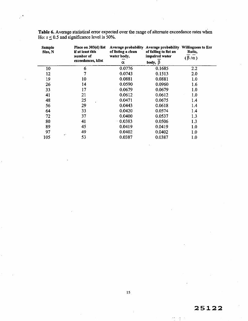
Table 6 shows the effect of binomial testing at the 50% confidence level with Ho: r 5 0.50. The willingness to err ratio now approaches unity with moderate sample sizes (say N>30). Because of the symmetry of power function graphs, this is the only test design that will balance both type of statistical errors.

The Policy's default one-sided null hypothesis attempts to put statistical control on alpha errors by testing at the 10% significance level. Beta errors are inversely related to the significance level. Therefore, if we lower the significance level of the test we will invariably increase beta errors. Conversely, if we increase the significance level we will decrease beta errors. The only way to simultaneously reduce alpha and beta errors is to increase the sample size.

References

Dixon, W. J. (1953). Powerfunctions of the sign test andpower ejiciency for normal alternatives. Annals of Mathematical Statistics 24:467-473.

Ellis, R. and D. Gulick. 1994. Calculus with analytic geometry. Saunders College Publishing, NY.

Gibbons, J. D. 1964. Effect of non-normality on thepowerfunction of the sign test. American Statistical Assoc. Joomal59:142-148.

Fig 1. Statistical alpha error and power associated with the binomial model for N=10, klist = 3, and a nominal significance level of 10%. Alpha error is the blue line function to the left of the 0.1 exceedance rate. Statistical power is the blue line function to the right of the 0.1 alternate exceedance rate.

Alt. Exceedance Rate

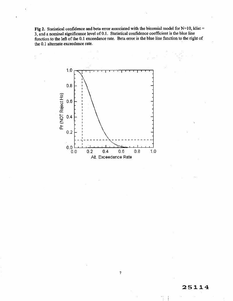
Fig 2. Statistical confidence and beta error associated with the binomial model for N=lO, klist = 3, and a nominal significance level of 0.1. Statistical confidence coefficient is the blue line function to the left of the 0.1 exceedance rate. Beta error is the blue line function to the right of the 0.1 alternate exceedance rate.

Alt. Exceedance Rate

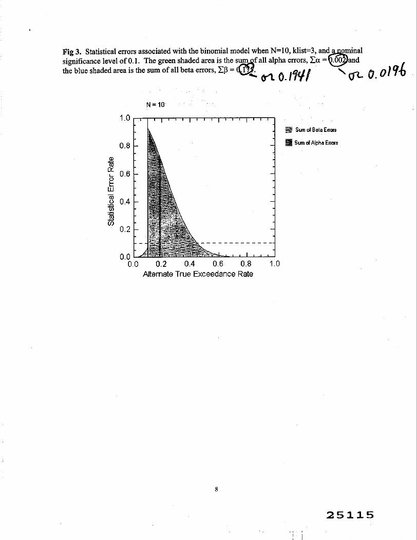
Fig 3. Statistical errors associated with the binomial model when N=10, klist=3, significance level of 0.1. The green shaded area is the the blue shaded area is the sum of all beta errors, ZP =

% Sum ol Beta Errors

Sum of Alpha Errors

Alternate True Exceedance Rate

Table 1. Reproduction of the Environmental Caucus's Table 1. Probabilities of making listing errors under the Draft Policy

Sample Place on 303(d) list Probability of Probability of Willingness to Err Size, N if at least this listing a clean failing to list an Ratio,

number of exceedances, klist

water body, a

impaired water body, 6

(Pla)

10 3 0.002 0.175 89 12 4 0.001 0.208 362 19 5 0.001 0.151 213 26 6 0.001 0.123 169 33 7 0.001 0.107 153 41 8 0.001 0.091 122 48 9 0.001 0.084 124 56 10 0.001 0.076 111 64 11 0.001 0.070 102 72 12 0.001 0.065 97 80 13 0.001 0.061 93 89 14 0.001 0.056 8 1 97 15 0.001 0.054 8 1

105 16 0.001 0.052 81

Table 2. Probability of rejecting the null hypothesis (Ho: r 5 0.1) for N = 10 and klist = 3. Average alpha = 0.0212, average power =0.8089, average beta = 1 - 0.8089 = 0.1911.

Alternate Decision P(reject Ho) P(N0T reject Ho) = l-exceedance rate, r If Ho is rejected P(reject Ho)

0.00 incorrect, alpha error 0.000 1.000 incorrect, alpha error incorrect, alpha error incorrect, alpha error incorrect, alpha error incorrect, alpha error incorrect, alpha error incorrect, alpha error incorrect, alpha error incorrect, alpha error incorrect, alpha error correct, power correct, power correct, power correct, power correct, power correct, power correct, power correct, power correct, power correct, power correct, power correct, power correct, power correct, power correct, power correct, power correct, power correct, power correct, power correct, power correct, power correct, power correct, power correct, power correct, power correct, power correct, power correct, power correct, power correct, power correct, power correct, power correct, power correct, power correct, power correct, power correct, power

correct, power correct, power m e e t , power correct, power correct, power correct, power correct, power correct, power correct, power correct, power correct, power correct, power correct, power correct, power correct, power correct, power correct, power correct, power correct, power correct, power correct, power correct, power correct, power correct, power correct, power correct, power correct, power correct, power correct, power correct, power correct, power correct, power correct, power correct, power correct, power correct, power correct, power correct, power correct, power correct, power correct, power correct, power correct, power correct, power correct, power correct, power correct, power correct, power correct, power correct, power correct, power correct, power

Table 3. Estimation of CP using Riemann sums. The interval [0.1, 11 on the x-axis of Figure 3 is partitioned into n subdivisionsof size Ar.

Number of Partitions, n Subdivision Size, A r 1 0 Approximation 4 0.25 0.1452 9 0.1 0.1297

90 0.01 0.1701 900 0.001 0.1752

9000 0.0001 0.1747 m lim Ar+O 0.175 (from Table 1)

Table 4. Table 1 recalculated using the average statistical error expected over the range of alternate exceedance values. Ho: r <0.1 and significance level is 10%.

Sample Place on 303(d) list if Average probability Average probability Willingness to Err Size, N at least this number of listing a clean of failing to list an Ratio,- -of exceedances, klist water body, -

a

impaired water

body, p (Pla)

10 3 0.0196 0.1941 9.9 12 4 0.0058 0.23 14 40.2 19 5 0.0071 0.1675 23.7 26 6 0.0073 0.1366 18.8 33 7 0.0070 0.1184 17.0 4 1 8 0.0075 0.1014 13.5 48 9 0.0068 0.0937 13.8 56 10 0.0069 0.0846 12.3 64 11 0.0069 0.0777 11.3 72 12 0.0067 0.0723 10.7 80 13 0.0066 0.0679 10.4 89 14 0.0069 0.0625 9.0 97 15 0.0067 0.0597 9.0

105 16 0.0064 0.0573 9.0

Table 5. Average statistical error expected over the range of alternate exceedance rates when Ho: r <0.05 and significance level is 50%.

Sample Place on 303(d) Average Average Willingness to Size, N list if at least this probability of probability of Err Ratio,

number of listing a clean failing to list an ( E l ; ) exceedances, klist water body, -

a impaired water body, F

10 1 0.2160 0.0544 0.25 12 1 0.2513 0.0416 0.17

- -

Table 6. Average statistical error expected over the range of alternate exceedance rates when Ho: r <0.5 and significance level is 50%.

Sample Place on 303(d) List Average probability Average probability Willingness to Err Size, N if at least this of listing a clean of failing to list an Ratio,

number of water body, impaired water exceedances, klist a

-body, p (Pla)

10 6 0.0776 0.1685 2.2 12 7 0.0743 0.1513 2.0 19 10 0.0881 0.0881 1.0 26 14 0.0590 0.0960 1.6 33 17 0.0679 0.0679 1.O 41 2 1 0.0612 0.0612 1.O 48 25 . 0.0471 0.0675 1.4 56 29 0.0443 0.0618 1.4 64 33 0.0420 0.0574 1.4 72 37 0.0400 0.0537 1.3 80 41 0.0383 0.0506 1.3 89 45 0.0419 0.0419 1.O 97 49 0.0402 0.0402 1.O

105 53 0.0387 0.0387 1.O