Evaluation of the effect of fines on asphalt concrete

Graduate Theses, Dissertations, and Problem Reports

2003

Evaluation of the effect of fines on asphalt concrete Evaluation of the effect of fines on asphalt concrete

Carlos Humberto Reyes West Virginia University

Follow this and additional works at: https://researchrepository.wvu.edu/etd

Recommended Citation Recommended Citation Reyes, Carlos Humberto, "Evaluation of the effect of fines on asphalt concrete" (2003). Graduate Theses, Dissertations, and Problem Reports. 1307. https://researchrepository.wvu.edu/etd/1307

This Thesis is protected by copyright and/or related rights. It has been brought to you by the The Research Repository @ WVU with permission from the rights-holder(s). You are free to use this Thesis in any way that is permitted by the copyright and related rights legislation that applies to your use. For other uses you must obtain permission from the rights-holder(s) directly, unless additional rights are indicated by a Creative Commons license in the record and/ or on the work itself. This Thesis has been accepted for inclusion in WVU Graduate Theses, Dissertations, and Problem Reports collection by an authorized administrator of The Research Repository @ WVU. For more information, please contact [email protected].

https://researchrepository.wvu.edu/

https://researchrepository.wvu.edu/

https://researchrepository.wvu.edu/etd

https://researchrepository.wvu.edu/etd?utm_source=researchrepository.wvu.edu%2Fetd%2F1307&utm_medium=PDF&utm_campaign=PDFCoverPages

https://researchrepository.wvu.edu/etd/1307?utm_source=researchrepository.wvu.edu%2Fetd%2F1307&utm_medium=PDF&utm_campaign=PDFCoverPages

mailto:[email protected]

EVALUATION OF THE EFFECT OF FINES ON ASPHALT CONCRETE

Carlos H. Reyes

Thesis submitted to the College of Engineering and Mineral Resources at West Virginia University in partial fulfillment of the

requirements for the degree of

Master of Science

In

Civil Engineering

Dr. John P. Zaniewski, Chair

Dr. Ronald W. Eck,

Dr. Jim French

Department of Civil and Environmental Engineering

Morgantown, West Virginia

2003

Keywords: Aggregate, Surface area, Mineral fillers, VMA, Aggregates,

Asphalt mix design, Volumetric analysis

The performance of asphalt surface pavements is directly affected by the

quality of the asphalt concrete. Several methods have been developed for

determining the quantities of aggregate and asphalt cement used in the asphalt

concrete. From the 1940’s to the present time, the Marshall method was widely

used in the United States. The Hveem method was in favor in some western

states. In the 1990’s, the SuperPave method was developed during the Strategic

Highway Research Program. With the support of the Federal Highway

Administration (FHWA), the SuperPave method is becoming widely implemented

(Roberts et. al, 1996). The common thread between the Marshall, Hveem and

SuperPave methods is the use of volumetric analysis to determine the

percentage of asphalt binder needed in an asphalt concrete mixture. The

volumetric criteria were developed for the asphalt concrete mixes with natural

sand as the fine aggregate. Currently, crushed fine aggregate are used in many

mixes. The influence of the differences in the specific surface area between

natural sand and the crushed fines has not been evaluated.

This research consists of the evaluation of the surface area of different

aggregates used in the state of West Virginia. This factor is important because

the amount of asphalt needed to coat the aggregate depends on the specific

surface area of the aggregate blend. The specific surface area of the aggregate

blend is usually calculated based on the aggregate gradation and surface area

factors.

This research proposes a method to obtain accurate specific surface area

factors using the Blaine air permeability apparatus. By using the factors

obtained, the voids in the mineral aggregate (VMA) and asphalt thickness are

calculated. The measured specific surface area of the crushed limestone fines is

much greater than the values computed using the traditional approach. This

implies that the asphalt concrete made with 100 percent crushed material will

have a much thinner asphalt film thickness than was considered adequate when

the volumetric mix design criteria were developed.

iii

ACKNOWLEDGMENT

The author would like to thank Dr. John Zaniewski, the author’s advisor for

his guidance and support during the pursuit of the author’s Master of Science

degree and participate in this research. The author would like to express his

gratitude to Dr. Ronald Eck and Dr. Jim French, the author’s committee

members.

Final thanks are given to Humberto Reyes, Rhaiza de Reyes, Jose Reyes

and Maria Del Bufalo, the author’s family, for their love and support. You are my

source of strength and motivation.

iv

TABLE OF CONTENTS Chapter 1 Introduction ..........................................................................................1

Introduction ................................................................................................1

Problem Statement ....................................................................................3

Objective ....................................................................................................4

Scope and Limitations................................................................................5

Thesis Overview.........................................................................................5

Chapter 2 Literature Review .................................................................................6

Introduction ................................................................................................6

Volumetric Criteria......................................................................................7

Volumetric Analysis..................................................................................10

Voids in the Mineral Aggregate ................................................................11

Specific Gravity of Aggregates .................................................................13

Specifc Gravity for Fine Aggregate ....................................................14

Specific Gravity for Mineral Filler and Baghouse Fines .....................16

Estimate Aggregate Effective Specific Gravity .........................................17

Aggregate Surface Area...........................................................................18

Methods for Estimating Surface Area ................................................18

Methods for Measuring Aggregate Surface Area...............................21

Asphalt Film Thickness ............................................................................25

Influence of Mineral Filler on Asphalt Concrete........................................25

Summary of Literature Review .................................................................26

Chapter 3 Research Approach ...........................................................................28

Samples Tested .......................................................................................28

Theoretical Analysis .................................................................................29

Evaluation of Particle Size........................................................................33

Gradations Used in Volumetric Analysis ..................................................34

Summary of Research Approach .............................................................35

Chapter 4 Data Collection and Analysis..............................................................38

Specific Gravity ........................................................................................38

Measured Specific Surface Area..............................................................39

v

Analysis Cases.........................................................................................42

Effect of Aggregate Size on Total Surface Area.......................................43

Volumetric Parameters.............................................................................47

Effect of Surface Area on Film Thickness ................................................54

Effect of Baghouse Fines .........................................................................54

Summary of Data Collection and Analysis ...............................................55

Chapter 5 Conclusions and Recommendations..................................................58

Conclusions..............................................................................................58

Recommendations ...................................................................................60

Reference ...........................................................................................................62

Specifications......................................................................................................64

Appendix A Specific Gravity of Samples.............................................................65

Appendix B Surface Area for the Material Pass 0.15mm and Retained on

0.075mm ..................................................................................................68

Appendix C Surface Area Pan Material ..............................................................75

Appendix D Baghouse Fines Specific Surface Areas .........................................82

Appendix E Volumetric Analysis Results ............................................................91

LIST OF FIGURES

Figure 2.1 Photo of Pycnometer Flask................................................................15

Figure 2.2 Photo of Le Chatelier Flask................................................................17

Figure 2.3 Air Permeability Apparatus (Blaine) ...................................................22

Figure 3.1 Gradations for NMAS 9.5 mm............................................................36

Figure 3.2 Gradations for NMAS 19 mm.............................................................37

Figure 4.1 Data sheet for Air Permeability Apparatus .........................................40

Figure 4.2 Method for the Calculation of Constant b...........................................41

Figure 4.4 Contribution of Size Material to Surface Area. Gradation #1 NMAS

19 mm. Craus-Ishai.......................................................................................45

Figure 4.5 Contribution of Size to Material to Surface Area. Gradation #1 NMAS

19 mm. Davg Method.....................................................................................46

vi

Figure 4.6 Contribution of Size to Material to Surface Area. Gradation #1 MNAS

19 mm. Natural Sand ....................................................................................46

Figure 4.7 Contribution of Size Material to Surface Area Gradation #1 NMAS

19 mm. Limestone Material...........................................................................47

Figure 4.8 VMA Values for 19 mm Mix #1 8µm Film Thickness..........................51

Figure 4.9 VMA Values for 19 mm Mix #1 2 µm Film Thickness.........................51

Figure 4.10 VFA Values for 19 mm NMAS #1 ....................................................52

Figure 4.11 VMA for 19 mm NMAS Gradations 2 µm Film Thickness. ...............52

Figure 4.12 VFA for 19 mm NMAS Gradations 2 µm. Film Thickness ................53

Figure 4.13 F/A for 19 mm NMAS Gradations 2 µm. Film Thickness .................53

Figure 4.14 MEASURED Surface Area vs. Film Thickness for a 19mm Mix.......55

Figure 4.15 Effect of Baghouse Fines Using Gradation #1 NMAS 19 mm for a

Film Thickness of 8 µm.................................................................................56

LIST OF TABLES

Table 2.1 Marshall Mix Criteria .............................................................................8

Table 2.2 SuperPave Mix Design Criteria .............................................................9

Table 2.3 Surface Area Factors Used by Hveem, Proposed by Edwards...........19

Table 2.4 Craus and Ishai Surface Area Factors ................................................19

Table 3.1 Assumptions for Mix Design................................................................32

Table 3.2 Gradation for a 19 mm Mix..................................................................32

Table 3.3 Volumetric Analysis for Mix Design.....................................................33

Table 3.4 9.5 mm Mix Designs Gradations for Asphalt Concrete .......................36

Table 3.5 19 mm Mix Designs Gradations for Asphalt Concrete ........................37

Table 4.1 Average Specific Surface Areas for Each Sample ..............................38

Table 4.2 Average Specific Surface Area for the Baghouse Fines .....................39

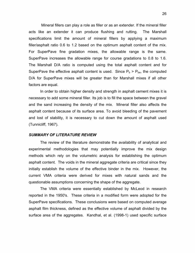
Table 4.3 Surface Area Factors used for the Volumetric Analysis ......................44

Table 4.4 Summary of the Volumetric Properties for 8 mm Film Thickness,

Edwards-Hveem Surface Area Factors.........................................................48

Table A.1 Specific gravities of the fine material evaluated..................................65

vii

Table A.2 Specific gravities of the baghouse material evaluated........................66

Table B.1 APAC sample # 2 surface area for the material pass 0.15 mm and

retained on 0.075 mm. ..................................................................................68

Table B.2 APAC Sample #1 surface area for the material pass 0.15 mm and

retained on 0.075 mm. ..................................................................................69

Table B.3 Summersville limestone surface area for the material pass 0.15 mm

and retained on 0.075 mm. ...........................................................................70

Table B.4 Beaver Boxley (A) surface area for the material pass 0.15 mm and

retained on 0.075 mm. ..................................................................................71

Table B.5 Beaver Boxley (B) surface area for the material pass 0.15 mm and

retained on 0.075 mm. ..................................................................................72

Table B.6 New Enterprise surface area for the material pass 0.15 mm and

retained on 0.075 mm. ..................................................................................73

Table B.7 Natural Sand surface area for the material pass 0.15 mm and retained

on 0.075 mm. ................................................................................................74

Table C.1 Summersville pan material Surface area............................................75

Table C.2 Beaver Boxley Sample (A) pan material surface area........................76

Table C.3 Beaver Boxley sample (B) pan material surface area ........................77

Table C.4 APAC sample #1pan material surface area........................................78

Table C.5 APAC Sample #2 pan material surface area ......................................79

Table C.6 New Enterprise pan material surface area .........................................80

Table C.7 Natural Sand pan material surface area.............................................81

Table D.1 Summersville baghouse fines specific surface area...........................82

Table D.2 Gasaway Baghouse fines specific surface area. ................................83

Table D.3 Beaver Boxley Baghouse fine sample (A) specific surface area ........84

Table D.4 Beaver Boxley baghouse fines sample (B) specific surface area .......85

Table D.5 APAC baghouse fine specific surface area ........................................86

Table D.6 J.F. Allen baghouse fines specific surface area .................................87

Table D.7 New Enterprise baghouse fines specific surface area........................88

Table D.8 W.V. Paving baghouse fines specific surface area.............................89

Table D.9 Tri-State baghouse fines specific surface area...................................90

viii

Table E.1 Volumetric analysis for 9.5 mm gradation #1......................................91




Table E.5 Volumetric analysis for 19 mm gradation #1.......................................95




ix

MASTER TABLE OF VARIABLE DEFINITIONS

b = Constant specifically determined for the test sample. bs = 0.9, the appropriate constant for the calibration sample. D = Density of the mercury at the test temperature Mg/m3. ε = Porosity of the test sample. εs = Porosity of prepared bed of the calibration sample. F = Factor 0.8 F/A = Fines to asphalt ratio Gb = Specific gravity of the binder Gmb = Bulk specific gravity of compacted mixture. Gmm = Maximum theoretical specific gravity of mixture. Gsa = Apparent specific gravity of the aggregate Gsb = Bulk specific gravity of the aggregate Gse = Effective specific gravity of the aggregate Gse = Effective specific gravity of the aggregate. η = Viscosity of air, µPa*sec, temperature of the test. ηs = Viscosity of air, µPa*sec, temperature of the calibration run. M = Mass of sample used (gm) Ms = Mass of aggregate (kg) P200 = Percentage of aggregate passing the #200 (0.075 mm) sieve. Pa = Percent air, assumed 4% Pb = percent binder Pba = Percent binder absorbed. Pbe = effective percent binder need equation Pbe = Percent effective binder Pi = Percent passing sieve i, in decimal form. Ps = Percent aggregate of stone. ρ = Density of the material (gm/cm3) ρs = Density of the standard sample. ρw = Density of water S = Specific surface Area (m2/kg) SA = Surface area ft2/lb or m2/kg SFi = Surface factor for sieve i

x

Ss = Specific surface of the standard sample, m2/kg T = Measured time interval, s, for test sample. Tb = Average thickness of binder (m) TF = Average Film Thickness, microns; Ts = Measured time interval, s, for calibration sample. V = Bulk volume of the calibration sample cm3 V = Bulk volume of the test sample (cm3), calculated using Equation 2.25. V = Volume of material (cm3) Vbe = Volume of binder (m3) Vbe = Effective volume of asphalt cement (liters) VFA = Voids fill with asphalt (%). Vm = Mix volume (m3) VMA = Voids in mineral aggregate (%). Vsb = Bulk volume of the aggregate (m3) VTM = Voids in total mix (%). Vv = Volume of air voids W = Weight of sample required (grams) WA = Weight of mercury used to fill the cell with no sample (gm). WB = Weight of mercury used to fill the cell with the sample (gm). Wbe = Weight of effective binder per unit weight of aggregate (kg binder/ kg aggregate)Ws = Mass of the stone, assumed 1 kg ρw = Density of water (grams/cm3)

1

CHAPTER 1 INTRODUCTION

INTRODUCTION

Over 90 percent of paved highways is the United States have a surface

where an asphalt cement is used as the binder agent. The preponderance of

these pavements are constructed with hot-mix asphalt concrete, HMAC. Asphalt

concrete is a mixture of the binder, aggregates and air. Based on empirical

evidence, the volume of air used in the mix design process is four percent.

Under the performance grade specifications, the base grade of binder is selected

based on the range of pavement temperatures expected for pavement’s service

conditions. The upper pavement temperature may be modified to account for

traffic loads and traffic speeds. Aggregates used in asphalt concrete may be

either natural sand, or crushed products, such as gravel and sand, or crushed

products. Aggregates are further categorized as coarse of fine depending on

whether the material is retained on or passes the 0.474 mm sieve. The

component of the aggregate material which passes the 0.075 mm sieve is

generally referred to as mineral filler or pan material.

The performance of asphalt surface roads is directly affected by the

quality of the asphalt concrete. Several methods have been developed for

determining the quantities of aggregate and asphalt cement used in the asphalt

concrete. From the 1940’s to the present time, the Marshall method was widely

used in the United States. The Hveem method was in favor in some western

states. In the 1990’s, the SuperPave method was developed during the Strategic

Highway Research Program. With the support of the Federal Highway

Administration, FHWA, the SuperPave method is becoming widely implemented

(Roberts, et al, 1996). The common thread between the Marshall, Hveem and

SuperPave methods is the use of volumetric analysis to determine the

percentage of asphalt binder needed in an asphalt concrete mixture.

2

Volumetric analysis uses data on the specific gravity of the aggregate and

the asphalt cement to determine volumetric parameters of the mix. The

parameters used in the mix design are:

• Voids in Total Mix, VTM.

• Voids in the Mineral Aggregate, VMA.

• Voids Filled with Asphalt, VFA.

McLeod originally established the criteria for these parameters in the

1950’s (McLeod, 1956). The criteria were refined and implemented into Marshall

method by the Asphalt Institute. The Marshall criteria were adopted into

SuperPave mix design method (Roberts, et al, 1996).

Natural sands and gravel were used in the fundamental research, which

established the volumetric criteria. McLeod’s evaluation of asphalt concrete

performance established that an effective asphalt content of 10 percent by

volume provided an optimum binder content. This analysis was based on

computing asphalt film thickness based on the specific surface area of the

aggregate. Specific surface area is the surface area per unit mass of the

aggregate. McLeod (1956) used specific surface area factors computed from the

specific gravity of the aggregate and the assumption that the aggregate are

spherical. It was also assumed that the aggregate’s diameter was equal to the

size of the sieve the aggregate passes through.

Researchers at the National Center for Asphalt Technology, NCAT,

evaluated McLeod’s work (Kandhal, et al, 1998). This research challenged the

methodology and criteria used in volumetric analysis. However, the NCAT

research used the same surface area factors as McLeod.

This research consists of the evaluation aggregates used in the state of

West Virginia. The specific surface area of the fine material was measured. This

factor is important because the amount of asphalt needed to coat the aggregate

depends on the specific surface area of the aggregate blend. The specific

surface area of the blend is usually calculated based on the aggregate gradation

and surface area factors. This involves multiplying the percentage aggregate

passing each sieve by the surface area factor for each sieve. These area factors

3

are obtained by assuming an aggregate specific gravity and that all the particles

are spheres or cube shaped. Using the length of the side of the opening for each

sieve, the surface area factors are determined using a simple equation. The

assumption of a spherical aggregate shape was developed when gravels and

natural sand were the predominant fine aggregate type used in asphalt concrete.

They have not been validated for crushed aggregates which are currently used in

asphalt concrete mixes.

PROBLEM STATEMENT

Asphalt concrete mix design requires the designer to select a combination

of aggregates, asphalt binder and air to produce a mix that meets criteria

established by the controlling agency. In West Virginia highway pavements are

constructed under the specifications developed by the Division of Highways,

WVDOH. These specifications were derived from national organizations

concerned with asphalt pavement construction. The WVDOH Marshall

specifications were adopted from the Asphalt Institute publication MS-2 (Asphalt

Institute, 1993). The WVDOH SuperPave specifications were adopted from

AASHTO specifications MP 2-99 (1999) for SuperPave volumetric design.

While many criteria must be satisfied under both the Marshall and

SuperPave mix design methods, one of the most challenging is the voids in the

mineral aggregate, VMA. This parameter represents the space between the

aggregate in the asphalt concrete. It is filled with the effective asphalt content

and air voids, or the voids in the total mix, VTM. Historically, it has been found

that a VTM in the range of three to five percent is required for durable concrete

mixes. For mix design, a VTM of four percent is required for SuperPave mixes

(WVDOH, 2000). Since the VTM is a constant, the VMA is then a measure of the

volume of effective binder in the mix. The binder film thickness is a function of

the volume of asphalt in the mix and the surface area of the aggregates. Since

the purpose of the binder is to coat and bind the aggregates together, the binder

film thickness is a key factor in asphalt concrete mix design.

4

The origin of the VMA criteria used in both the Marshall and SuperPave

mix design methods can be traced back to research performed by Norman

McLeod in 1956 (McLeod, 1956). McLeod researched the behavior and

performance of mixes with natural sand as the fine aggregate. Currently, West

Virginia, as well as many other states, use crushed limestone fine aggregates for

many of their mixes. Depending on haul distance, crushed limestone fine

aggregate may be more economical than natural sand. Furthermore, use of

natural sand is effectively limited under the SuperPave consensus aggregate

criteria for fine aggregate angularity. The differences in the shape and texture of

natural sand versus crushed limestone fine aggregate, leads to the question of

whether or not the volumetric criteria developed for natural sands is appropriate

for crushed limestone fine aggregate.

OBJECTIVE

The objective of this research is to evaluate the effect of aggregate

surface area on the selection of the optimum asphalt content. Aggregate specific

surface area is not currently an explicit design criterion in either the SuperPave

or Marshall mix design methods. However, specific surface area is the

controlling factor in determining asphalt film thickness. The VMA criterion

effectively controls the minimum asphalt film thickness. Since the VMA criteria

were developed for natural sand mixes, evaluation of the criteria for the crushed

limestone sand mixes were evaluated.

Existing models of specific surface area assume the aggregate particles

are spherical and the effect texture is not considered. To support the main

objective of the research, a direct measure of the specific surface area was

sought. Due to the sensitivity of specific surface area on fine materials, the

specific surface area of the aggregate passing the 0.15 mm sieve were

measured in the laboratory. These evaluations were performed for a range of

aggregates used in West Virginia.

5

SCOPE AND LIMITATIONS

The research reported herein focuses on aggregate materials and

procedures that are used for the design of mixes for the West Virginia Division of

Highways. The materials selected for the study were samples from stockpiles

across the state of West Virginia. Six samples of crushed limestone fine

aggregate and one sample of natural sand were used in the study. In addition,

nine samples of baghouse fines were collected and evaluated. Baghouse fines

is the fine material that is separated from the aggregate when the aggregates are

dried for the production of asphalt concrete.

The results produced in this research were based on the volumetric

analysis for hot-mix asphalt concrete. These results are theoretical. These

results were not verified with experimentation.

The specific surface area, surface area per unit mass, of materials is a

function of the particle size. Small particles have a greater specific surface area

than large particles. This research focused on measuring the surface area of

particles that pass the 0.15 mm sieve. The specific surface area of the material

finer than the 0.15 mm sieve is much greater than the specific surface area of

larger size aggregates. Hence, the research focused on measurements of these

surface areas.

Equipment for measuring the surface area of larger aggregates was not

available for the research. Surface area of the aggregates were estimated using

the traditional method. Any error resulting from this approach is mitigated by the

fact that the larger aggregates contribute little to the total surface area of the

aggregates in the mix.

THESIS OVERVIEW

This thesis is organized into five chapters and five appendixes. Following

this introductory chapter, a review of the literature is presented in Chapter 2. The

research approach is described in Chapter 3. The data collected during the

research and the subsequent analysis are presented in Chapter 4. Conclusions

and recommendation are presented in Chapter 5

6

CHAPTER 2 LITERATURE REVIEW

INTRODUCTION

The research presented herein builds on volumetric concepts, which are

well established in the literature. The volumetric criteria used by the West

Virginia Department of Transportation, WVDOT, are presented since they control

mix designs in the region of interest. However, the WVDOT criteria are based on

the recommendations of the Asphalt Institute and the America Association of

State Highways and Transportation Officials, AASHTO, for the Marshall and

SuperPave methods, respectively. Hence, the scope of the research has nation

wide applications.

The volumetric criteria are followed by a presentation of the equation used

for volumetric analysis. These relationships can be derived from the definitions

of the volumetric terms. However, the relationships are well documented in the

literature. Hence they are presented rather than derived herein.

The volumetric parameter, which controls the minimum asphalt content, is

the voids in the mineral aggregate, VMA. The literature for establishing the VMA

criteria is documented due to the importance of this parameter on mix designs.

In a NCAT study, the relationships between volumetric parameters and the

asphalt film thickness were derived. These equations are presented since they

are fundamental to the research presented herein.

Volumetric analysis is dependent on the determination of specific gravity

of the materials. The procedures for measuring the specific gravity of the fine

aggregates and mineral fillers and baghouse fines are presented to document

the test methods used during the research.

The ASTM method for measuring the specific gravity of portland cement

was used to measure the specific gravity of the mineral fillers and the baghouse

fines. This was necessary since there is not a specific test method for measuring

the specific gravity of these materials.

7

As documented in this chapter, the volume of effective binder in asphalt

concrete can be computed from film thickness criteria, gradation, and the specific

surface area factors. However, estimating total asphalt content requires an

estimate of the amount of absorbed asphalt. This is normally evaluated after

mixing the asphalt concrete. The FHWA has presented an equation for

estimating the effective specific gravity of the aggregates as a function of the bulk

and the apparent specific gravity. The percent absorbed binder can then be

computed from the effective and the bulk specific gravity of the aggregate and

the specific gravity of the binder content.

Evaluation of the aggregate specific surface area is necessary for

evaluating asphalt film thickness. Several authors have addressed this topic,

starting with Hveem in 1942 (Campen, et al, 1959). Historically, specific surface

area was computed based on an assumed aggregate shape. The work of

asphalt technologists using this approach is documented. However, the specific

surface area of the fine materials can be measured using techniques developed

in the portland cement industry. The Blaine finesse meter is one such device

and it was used to measure the specific surface area of the aggregate materials

finer than 0.15 mm. The test method for using the Blaine fineness meter is

documented.

The final section of the literature review documents the equations

developed by Kandhal et al (1998-1) for estimating film thickness from the

volume of effective binder, specific surface area and the mass of the aggregate

in a mix.

VOLUMETRIC CRITERIA

Volumetric analysis is used to determine the volume of asphalt and

aggregates needed to make an asphalt mix with the desired properties.

However, it is impractical to measure aggregate volumes in a production

environment. Therefore, the mass and density of the materials are used to

compute volumetric properties. The volumetric parameters controlled in both the

Marshall and SuperPave mix design methods are the voids in total mix (VTM),

8

voids in the mineral aggregate (VMA), voids filled with asphalt (VFA) and the dust

to asphalt ratio. The WVDOH volumetric mix design requirements are given in

Tables 2.1 and 2.2 for the Marshall (WVDOT MP 402.02.22.2000) and

SuperPave (WVDOT MP 402.02.28.2000) mix design methods respectively.

TABLE 2.1 MARSHALL MIX CRITERIA

Compaction, number of blows, Each end of

specimen50 75 112

Stability, (Newtons) Minimum 5,300 8,000 13,300

Flow, (0.25 mm) 8 - 16 8 - 14 12 - 21Air Voids (%) Design based on a midpoint

of a range3 - 5 3 - 5 3 - 6

Voids Filled with Asphalt (%) 65 - 78 65 - 75 63 - 75

VMA (%) 15 13 11

Design Criteria (1)Wearing I Medium

Traffic Design

Base II Heavy Traffic Design

Base I Heavy Traffic Design

Notes

1. The fines-to-asphalt ratio shall be within the range of 0.6 to 1.2

based on the asphalt content of the mix.

9

TABLE 2.2 SUPERPAVE MIX DESIGN CRITERIA

4%0.6 - 1.280% min

37.5mm 25mm 19mm 12.5mm 9.5mm

11 12 13 14 15

NinitialNdesig

n Nmax<0.3 ≤91.5 96 ≤98.0

0.3 - 3 ≤90.5 96 ≤98.03 - 10 ≤89.0 96 ≤98.0

10 - 30 ≤89.0 96 ≤98.0≥30 ≤89.0 96 ≤98.0

Design Air VoidsFines to Effective Asphalt1

Tensile strength ratio2

Nominal Maximum Size

65-75

Minimum Voids in the Mineral Aggregate

70-8065-7865-7565-75

Design EASL millions

Percent Maximum Theoretical Specific

GravityVoids Filled with

Asphalt3,4,5

Notes

2. Dust to binder range 0.8 to 1.6 for coarse aggregate blends.

3. If mix fails, use an approved antistrip and redesign with antistrip in

the mix. All design tests must be with the antistrip in the mix.

4. For 9.5 nominal maximum aggregate size mixes and design ESAL

≥ 3 million, VFA range is 73 to 76 percent.

5. For 25 mm nominal maximum aggregate size mixes, the lower limit

of the VFA range shall be 64% for design traffic levels <.3 million

ESALs.

6. For 37.5 mm nominal maximum aggregate size mixes, the lower

limit of the VFA range shall be 64% for all design traffic levels.

10

VOLUMETRIC ANALYSIS

The volumetric analysis consists of computing volumetric parameters from

laboratory tests. Aggregate bulk and apparent specific gravity are measured

using AASHTO T84-94 and T85-91 methods for fine and course aggregates,

respectively. The specific gravity of the asphalt cement is measured using

AASHTO 228-94 method. The bulk and maximum theoretical specific gravity of

the asphalt concrete are measured using AASHTO T166-06 and T209-99,

respectively. Once these parameters are measured, the volumetric analysis is

performed using the equations (Roberts, et al, 1996):

−=

mm

mb

GG

VTM 1100 2.1

×

−−= 100)1(100

sb

bmb

GPGVMA 2.2

−

=VMAVMTVMAVFA 100 2.3

bP200PF/A = 2.4

beP200P

F/A = 2.5

The percent effective binder Pbe, is computed as:

sba

bbe PPPP ×−=100

2.6

bs PP −= 100 2.7

bsbse

sbseba G

GGGGP ×

×−

= 100 2.8

11

b

b

mm

bse

GP

G

PG−

−= 100100 2.9

Where:

VTM = Voids in total mix (%).

VMA = Voids in mineral aggregate (%).

VFA = Voids fill with asphalt (%).

Gsb = Bulk specific gravity of aggregate.

Gmb = Bulk specific gravity of compacted mixture.

Gmm = Maximum theoretical specific gravity of mixture.

F/A = Fines to asphalt ratio

P200 = Percentage of aggregate passing the #200 (0.075 mm) sieve.

Pb = Percent binder

Pbe = Effective percent binder need equation

Pba = Percent binder absorbed.

Ps = Percent aggregate of stone.

Gse = Effective specific gravity of the aggregate.

Equation 2.4 is used for the Marshall method and Equation 2.5 is used for

the SuperPave method.

VOIDS IN THE MINERAL AGGREGATE

The design and study of asphalt-paving mixtures was based on the

volumetric considerations since the topic was introduced N. W. McLeod in 1956

(McLeod, 1956). McLeod's analysis was based on a relation between the

volumes of the total aggregate, the asphalt binder and the air voids in the

mixture. The specific gravity of the asphalt cement and aggregates were 1.01

and 2.65, respectively. McLeod (1956), working with aggregates with 100

percent passing the 3/4" sieve, 5 percent air voids and a minimum of 10 percent

binder by volume. This resulted in the recommendation for a minimum of 15

percent voids in the mineral aggregate.

12

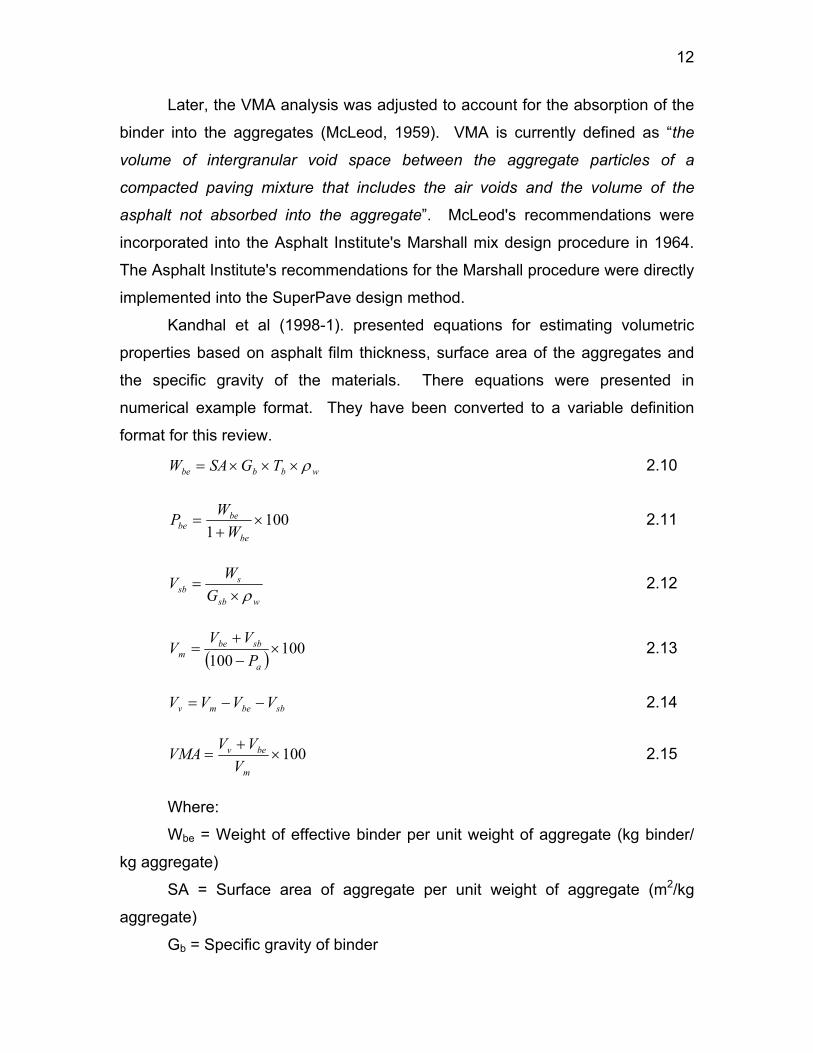
Later, the VMA analysis was adjusted to account for the absorption of the

binder into the aggregates (McLeod, 1959). VMA is currently defined as “the

volume of intergranular void space between the aggregate particles of a

compacted paving mixture that includes the air voids and the volume of the

asphalt not absorbed into the aggregate”. McLeod's recommendations were

incorporated into the Asphalt Institute's Marshall mix design procedure in 1964.

The Asphalt Institute's recommendations for the Marshall procedure were directly

implemented into the SuperPave design method.

Kandhal et al (1998-1). presented equations for estimating volumetric

properties based on asphalt film thickness, surface area of the aggregates and

the specific gravity of the materials. There equations were presented in

numerical example format. They have been converted to a variable definition

format for this review.

wbbbe TGSAW ρ×××= 2.10

1001

×+

=be

bebe W

WP 2.11

wsb

ssb G

WVρ×

= 2.12

( ) 100100

×−+

=a

sbbem P

VVV 2.13

sbbemv VVVV −−= 2.14

100×+

=m

bev

VVVVMA 2.15

Where:

Wbe = Weight of effective binder per unit weight of aggregate (kg binder/

kg aggregate)

SA = Surface area of aggregate per unit weight of aggregate (m2/kg

aggregate)

Gb = Specific gravity of binder

13

Tb = Average thickness of binder (m)

Pbe = Percent effective binder

Ws = Mass of the stone, assumed 1 kg

Vbe = Volume of effective binder (m3)

Vsb = Bulk volume of the aggregate (m3)

Gsb = Bulk specific gravity of the aggregate

Vm = Mix volume (m3)

Pa = Percent air, assumed 4%

Vv = Volume of air voids

ρw = Density of water

It should be noted that Equation 2.11 is based on effective binder content.

Traditionally, Pbe is based on total asphalt content i.e. the denominator of

equation 2.11 is traditionally (Ws + Wbe + Wba). These equations assume the

density of water is 1 gm/cc so the differences between specific gravity and

density can be numerically ignored.

SPECIFIC GRAVITY OF AGGREGATES

Due to the surface voids of aggregates, several definitions of specific

gravity have been developed to account for the treatment of the volume of the

voids at the aggregate surface. The apparent specific gravity, Gsa, is the mass of

the material divided by the volume of the aggregate, including internal impervious

voids. However, the surface voids of aggregates are too small to impact the

packing of aggregates in an asphalt concrete mix. Therefore, the bulk specific

gravity, Gsb, is defined as the mass of the material divided by the volume of the

material plus the volume of the surface voids. Finally, since asphalt cement

cannot fill the surface voids as effectively as water, the effective specific gravity,

Gse, is defined as the mass of the material divided by the volume of the material,

plus the volume of the surface voids, minus the volume of the voids filled with

asphalt.

Due to the range of aggregate sizes, different test methods are required

for determining specific gravity. Coarse aggregates were not considered in this

14

research so the test method is not presented. The specific gravity of fine

aggregates is determined with ASTM C 128-01. This method is applied to the

fine materials with the mineral fillers present. However, due to the significance of

the specific gravity of mineral filler and baghouse fines in this research, a test

method for measuring their specific gravity directly was sought. ASTM C 188-95

covers measuring the density of hydraulic cements. Since the particle size of the

mineral fillers and hydraulic cement is similar, this method was used to check the

specific gravity of the mineral fillers.

SPECIFC GRAVITY FOR FINE AGGREGATE

ASTM C 128-01 requires drying of the aggregate, then immersion in water

for 15 to 19 hours, drying the sample to the Saturated Surface Dry, SSD,

condition. The mass of the sample is measured in the SSD condition,

submerged in water and after drying to a constant weight. The SSD condition is

determined using a specified conical mold and a tamper. The material is placed

in the cone, tamped twenty five times and the cone is removed. If the material

slumps, the SSD condition is reached, but if it does not slump it is necessary to

dry the sample further.

After reaching the SSD condition, 500 ± 1 grams of the sample are placed

in a pycnometer (Figure 2.4) charged with water. All air voids are removed and

the pycnometer is filled with water to the calibration line. The mass is recorded.

The material is taken out and placed in the oven at a temperature of 110 oC for

drying. The mass of the dry material is determined.

The following formulas are used compute specific gravity and absorption:

Bulk Specific Gravity (Oven Dry basis)

CDBAGsb −+

= 2.16

Bulk Specific Gravity (SSD Basis)

CDBDG

SSDsb −+= 2.17

15

FIGURE 2.1 PHOTO OF PYCNOMETER FLASK.

Apparent Specific Gravity

CABAGsa −+

= 2.18

Absorption 100×−

=AAD 2.19

Where:

A = Mass of oven-dry sample in air, grams

B = Mass of pycnometer filled to calibration mark, grams.

C = Mass of pycnometer, sample, and water to calibration mark, grams.

D = Mass of saturated-surface-dry sample in air, grams.

16

SPECIFIC GRAVITY FOR MINERAL FILLER AND BAGHOUSE FINES

There is not a specific test method for determining the specific gravity of

mineral fillers and baghouse fines. ASTM C 188-95, Standard Test Method for

Density of the Hydraulic Cement, was used to measure the density of the

baghouse fines due to the fineness of the material. This method was also used

to determine the specific gravity of the mineral filler of some samples.

ASTM C 188-95 uses a LeChatelier flask (shown in Figure 2.2) to directly

measure the volume of a sample of material. The flask is filled with kerosene

between the 0 and 1 ml marks. It is then placed in a water bath at a temperature

of 23 ± 2oC. Then about 60 grams of the material is introduced in the flask.

While adding the material, it is necessary to check that no material adheres to

the walls of the flask. After the material is added, the flask is placed in an inclined

position and rotated to evacuate all air. Finally, the flask is placed back in the

water bath and the temperature is equilibrated to be with in ±0.2°C of the

temperature during the initial volume measurement. The second volume

measurement is recorded.

The density is calculated as:

VM

=ρ 2.20

Where:

ρ = Density of the material (gm/cm3)

M = Mass of sample used (gm)

V = Volume of material (cm3)

17

FIGURE 2.2 PHOTO OF LE CHATELIER FLASK

ESTIMATE AGGREGATE EFFECTIVE SPECIFIC GRAVITY

The effective specific gravity of an aggregate must be known in order to

determine the absorbed asphalt content. This can be computed if the percent

binder, specific gravity of the binder and the maximum theoretical specific gravity

of the mix is known, as shown in Equation 2.9. However, the U.S. Department of

Transportation (Harman et al, 1999) presents a equation where an estimate of

the effective specific gravity, Gse, is obtained from the bulk specific gravity, Gsb,

and the apparent specific gravity, Gsa, of an aggregate.

( sbsasbse GGFGG −+= ) 2.21

Where:

Gse = Effective specific gravity of the aggregate

Gsb = Bulk specific gravity

Gsa = Apparent specific gravity of the aggregate

18

F = Factor 0.8

The factor of 0.8 is to compensate the difference between the absorption

of water in relation to the absorption of the asphalt binder.

AGGREGATE SURFACE AREA

METHODS FOR ESTIMATING SURFACE AREA

Hveem developed a method for estimating the surface area of aggregates

based on gradation using surface areas factors proposed by L. N. Edwards

(Roberts, et al, 1996). These factors are based on the diameter of the aggregate

that is equivalent to the size or the opening of the sieve. Edwards reportedly

represented the aggregates as spheres. Edwards surface area factors are

presented in Table 2.3.

The surface area per unit mass for an aggregate blend is determined by

summing the product of the surface area factor times the percent material

passing each sieve size (Roberts, et. al, 1996), expressed mathematically as:

∑ ×= ii PSFSA 2.22

Where

SA = Surface area ft2/lb or m2/kg

SFi = Surface factor for sieve i

Pi = Percent passing sieve i, in decimal form.

The surface area factor for all sieves greater than 4.75 mm is applied to

the sieve corresponding to the maximum aggregate size and therefore P1 is

always 1.00.

An inherent assumption of Hveem's method for computing surface area is

that the particles are spheres with smooth sides. Craus and Ishai (1977)

performed a literature review on the effects of this assumption and concluded

that Hveem's method provided reasonable approximations of surface area.

19

TABLE 2.3 SURFACE AREA FACTORS USED BY HVEEM, PROPOSED BY

EDWARDS

Sieve Size # >#4 # 4 # 8 # 16 # 30 # 50 # 100 # 200

Diameter (mm) 4.75 2.36 1.18 0.60 0.30 0.15 0.075

Surface Area (m2/kg) 0.41 0.41 0.82 1.64 2.87 6.14 12.29 32.77

Surface Area (ft2/lb) 2 2 4 8 14 30 60 160

Craus and Ishai (1977) assumed that all particles have a sphere or a cube

form with D being the diameter or length of the edge and ρ the density of the

aggregate in kg/m3 to calculate the surface area (S) in m2/kg as:

DS

⋅=

ρ6 2.23

Table 2.4 presents the surface area factors for a specific gravity of 2.65.

These values are somewhat different than the surface area factors presented by

Hveem. The reasons for this discrepancy are not described in the literature.

TABLE 2.4 CRAUS AND ISHAI SURFACE AREA FACTORS

Sieve # # 4 # 8 # 16 # 30 # 50 # 100 # 200

D (mm) 4.75 2.36 1.18 0.6 0.3 0.15 0.075

Surface Area (m2/kg) 0.48 0.96 1.90 3.77 7.55 15.10 30.20

Surface Area (ft2/lb) 2.33 4.68 9.37 18.42 36.85 73.70 147.40

Duriez and Arrambide propose another method for the calculation of

surface area (Duriez 1962). This method is being used in France and consists on

applying the following formula:

20

CBAS ⋅+⋅+⋅= 3.212135 2.24

Where:

S = Specific surface area (m2/kg)

A = Percentage by weight of the fraction finer than 80 µm

B = Percentage by weight in the range between 80 µm – 0.315 mm

C = Percentage by weight in the range between 0.315 mm – 5.0 mm

Equation 2.24 is similar to Equation 2.22 if only three sieve sizes are

considered. The coefficient for the fine material, passing the 80 µm sieve should

be similar to the surface area factors for material passing the 75 µm. However,

the Edwards-Hveem and Cruas-Ishai factors are approximately one quarter of

the Duriez-Arrambide values.

Chapuis and Legare (1992) evaluated the Hveem-Edwards, Duriez-

Arrambide and Craus-Ishai methods for a clean sand with 2 percent mineral filler.

Based on this analysis, they recommended computing surface area based on the

edge dimension of the retaining sieve and the percent retained on the sieve, i.e.:

∑ −=

i

NodNoD

dPPS

ρ6 2.25

Comparison of this method for computing surface area of sands to the

other methods demonstrated that it produced similar estimates to the Craus-Ishai

method but estimated a higher surface area than either the Hveem-Edwards or

Duriez-Arrambide methods.

Chapuis and Legare (1992) used two methods for determining the surface

area of mineral fillers. One method used sieving of the mineral fillers and

Equation 2.25 to compute the specific surface area. The other method measured

specific surface area of mineral fillers using the Blaine air permeability apparatus

(ASTM C204). The resulting values for specific surface area of mineral fillers

were:

21

Material Computed Surface Area (m2/kg)

Measured Surface Area (m2/kg)

Limestone 325 263 Dolomite 206 202 Basalt 247 247

The measured and computed values are very close for the dolomite and basalt

mineral fillers. The limestone values are different by 22.9 percent. In all cases,

the surface areas are much greater than the Hveem-Edwards surface area factor

of 32.77. The authors did not state if these materials were manufactured by

crushing. However, based on the geological classification of the rocks it would

be reasonable to assume the materials were produced by crushing.

METHODS FOR MEASURING AGGREGATE SURFACE AREA

There are several tests for the measurement of surface area of fine

materials. The surface area for hydraulic cement is used as a quality control

measure. The Blaine air permeability apparatus, shown in Figure 2.3, and the

Wagner turbidimeter are commonly used ASTM procedures. The Blaine method

was used in this research, so this procedure is explained. This is also the

method used by Chapuis and Legare (1992).

The basic procedure for using the Blaine air permeability apparatus,

ASTM C-204, consists of placing a bed of material, with a specific porosity, in the

permeability cell. A vacuum is used to force air through the sample to a

manometer which measures the vacuum. The time required to cause a change

in the manometer reading from the initial point to a final point is related to the

size of the particles, at a specific porosity.

For calibration, the bulk volume of the compacted bed is measured using

a National Institute of Standards standard material No. 114. This is a portland

cement material with independently determined specific surface area. The

specific surface area of the calibration sample used was 396.6 m2/kg.

22

FIGURE 2.3 AIR PERMEABILITY APPARATUS (BLAINE)

The volume occupied by the calibration material is obtained by placing two

filters completely over the perforated metal disk located at the bottom of the

permeability cell. Then the permeability cell is filled with mercury, a plate of glass

is used to level it, making sure there is no air voids between the mercury and the

glass. The mercury is taken out of the cell and its weight is determined. The

next step is to place a new filter in the cell and 2.8 gm of the standard material is

added to the cell and covered with a filter. The rest of the cell is filled with

mercury and leveled as explained before. The new weight of the mercury is

measured. The following formula is used to calculate the bulk volume of the

calibration material:

DWWV BA )( −= 2.26

Where:

23

V = Bulk volume of the calibration sample cm3.

WA = Weight of mercury used to fill the cell with no sample (gm).

WB = Weight of mercury used to fill the cell with the sample (gm).

D = Density of the mercury at the test temperature Mg/m3.

The procedure is repeated two times and the average of the volume is

used for calculating the weight of the test samples.

The preparation of the test sample starts by enclosing it in a jar and

shaking for two minutes. It is allowed to rest for another two minutes. This is

done to break up the lumps and agglomerates. The required weight of the test

sample is estimated as:

)1( ερ −⋅⋅= VW 2.27

Where:

W = Weight of sample required (grams)

ρ = Density of the test sample (grams/cm3)

V = Bulk volume of the test sample (cm3), calculated using Equation 2.26.

ε = Porosity of the test sample.

Porosity is the ratio of the volume of voids in the sample divided by the

bulk volume of the sample.

The bed of test sample is prepared by placing the perforated disk and a

paper filter in the cell. The sample with a weight calculated with Equation 2.27 is

placed in the cell. Another filter is added on the top and pressed down using the

plunger until the collar of the plunger touches the top of the cell. The plunger is

removed, rotated 90o and pressed again.

The cell is to connected to the manometer. Air is evacuated from one arm

of the tube, bringing the oil to the top mark. The vacuum is released and the time

for the liquid to go from the second mark to the third mark is measured. The time

and temperature are recorded.

For the each test sample, three measurements of time are made for four

different levels of porosity. Using the recorded times and temperatures, and the

24

data obtained during calibration the specific surface area is computed using

Equation 2.28 or 2.29. Equation 2.28 is used when the temperature range is

within ±3oC of the calibration temperature and 2.29 otherwise.

ss

ssss

Teb

TbSS

3

3

)(

)(

ερ

εερ

−

−= 2.28

ηερ

εηερ

ss

sssss

Teb

TbSS

3

3

)(

)(

−

−= 2.29

Where:

S = Specific surface of the test sample, m2/kg.

Ss = Specific surface of the standard sample, m2/kg

T = Measured time interval, s, for test sample.

Ts = Measured time interval, s, for calibration sample.

η = Viscosity of air, µPa*sec, temperature of the test.

ηs = Viscosity of air, µPa*sec, temperature of the calibration run.

ε = Porosity of prepared bed of test sample.

εs = Porosity of prepared bed of the calibration sample.

ρ = Density of the test sample.

ρs = Density of the standard sample.

b = Constant specifically determined for the test sample.

bs = 0.9, the appropriate constant for the calibration sample.

The value of b is calculated by measuring the times of three samples of

the material for each of the four porosities. The values of T3ε and ε are plotted

and the intersection of the best-fit regression line with the Y-axis is b. If the

correlation coefficient between T3ε and ε is higher than 0.997, the b value is

accepted and the specific surface area can be calculated. If the correlation

25

coefficient is less than 0.997 the data are discarded and a new set of samples is

evaluated.

ASPHALT FILM THICKNESS

Asphalt film thickness is not directly considered for the design of asphalt

concrete. However, research has demonstrated that a desirable coat is needed

over the aggregate particles to ensure the performance of the asphalt concrete.

A method to calculate the film thickness of an asphalt mix, based on the

surface area factors, was developed by Hveem. The following formula is used to

calculated the film thickness (Roberts, et. al, 1996):

ws

beF MSA

VT ρ××

= 2.30

Where:

TF = Average Film Thickness, microns;

Vbe = Effective volume of asphalt cement (liters)

SA = Specific surface area of the aggregate (m2/kg)

Ms = Mass of aggregate (kg)

ρw = Density of water (grams/cm3)

Campen et al. (1959) recognized the relationship between voids,

aggregate surface area, binder film thickness and stability for dense graded

asphalt concrete mixes. A recommendation of an average asphalt film thickness

of 6 to 8 microns was needed for flexible and durable asphalt mixtures. Thinner

asphalt films results in mixes that are likely to break, crack, and ravel. An 8 µm

film thickness was also recommended by NCAT researchers (Kandhal et.al,

1998-1).

INFLUENCE OF MINERAL FILLER ON ASPHALT CONCRETE

Kandhal (1998-2) reviewed several studies which demonstrated that the

properties of the asphalt concrete are strongly influenced by the material passing

the 0.075 mm sieve. This material is generally referred to mineral filler.

26

Mineral fillers can play a role as filler or as an extender. If the mineral filler

acts like an extender it can produce flushing and rutting. The Marshall

specifications limit the amount of mineral fillers by applying a maximum

filler/asphalt ratio 0.6 to 1.2 based on the optimum asphalt content of the mix.

For SuperPave fine gradation mixes, the allowable range is the same.

SuperPave increases the allowable range for course gradations to 0.8 to 1.6.

The Marshall D/A ratio is computed using the total asphalt content and for

SuperPave the effective asphalt content is used. Since Pb > Pbe, the computed

D/A for SuperPave mixes will be greater than for Marshall mixes if all other

factors are equal.

In order to obtain higher density and strength in asphalt cement mixes it is

necessary to add some mineral filler. Its job is to fill the space between the gravel

and the sand increasing the density of the mix. Mineral filler also affects the

asphalt content because of its surface area. To avoid bleeding of the pavement

and lost of stability, it is necessary to cut down the amount of asphalt used

(Tunnicliff, 1967).

SUMMARY OF LITERATURE REVIEW

The review of the literature demonstrate the availability of analytical and

experimental methodologies that may potentially improve the mix design

methods which rely on the volumetric analysis for establishing the optimum

asphalt content. The voids in the mineral aggregate criteria are critical since they

initially establish the volume of the effective binder in the mix. However, the

current VMA criteria were derived for mixes with natural sands and the

questionable assumptions concerning the shape of the aggregate.

The VMA criteria were essentially established by McLeod in research

reported in the 1950's. These criteria in a modified form were adopted for the

SuperPave specifications. These conclusions were based on computed average

asphalt film thickness, defined as the effective volume of asphalt divided by the

surface area of the aggregates. Kandhal, et al. (1998-1) used specific surface

27

area factors developed by Edwards, which assumed the aggregate particles are

smooth sided spheres.

Edwards-Hveem and Craus-Ishai methods to determine specific surface

area are based on the same assumption, but the factors obtained are not equal.

The reason for this discrepancy is not described in the literature. Craus- Ishai

values can be confirmed with calculations. The surface area factors were

derived with the assumption that aggregates are spheres with the diameter equal

to the size of the sieve through which the aggregate passes. These surface area

factors were not experimentally validated. There is evidence from Duriez and

Arrambide that the computed surface area factors for sand material finer than

0.075 mm may be in error by a factor of four. Chapuis and Legare present

evidence that the Hveem-Edwards surface area factors are incorrect by a factor

of 6 to 10, depending on mineralogy, for mineral fillers from crushed materials.

They also demonstrated that the Blaine air permeability apparatus is a viable

method for evaluating surface area of these materials.

28

CHAPTER 3 RESEARCH APPROACH

The objective of this research is to evaluate the effect of aggregate

surface area on the selection of the optimum asphalt content. Applying the

volumetric analysis for different film thickness for the mix design and values such

as VMA, VTM, VFA and fines-asphalt ratio are examined with the purpose to

determined the influence of the specific surface area. The analytical method for

computing asphalt film thickness requires estimates of specific surface area of

the aggregates. The literature review demonstrates a discrepancy between the

computed and measured surface area factors for fine materials. Therefore, a

laboratory method was used for measuring the surface are of the material finer

than 0.15 mm.

The research approach involved obtaining samples of fine materials from

various sources throughout the state of West Virginia. The specific surface areas

of the samples were evaluated with a Blaine air permeability apparatus. Then

using analytical methods set forth by Kandhal et al. (1998-1) the implications of

the measured surface area on the film thickness and VMA were evaluated.

SAMPLES TESTED

The samples used the research were provided by eight asphalt plants

which provide asphalt concrete for the West Virginia Division of Highways. The

suppliers provided samples of fine aggregate and baghouse fines. The following

asphalt plants provided the samples for the research. The specific gravities are

presented in Table A.1 in the Appendix A.

• APAC – Virginia, Inc.

• J.F. Allen Company

• Meadows Stone & Paving, Inc.

• New Enterprise Stone & Lime Co. Inc.

• Tri-State Company.

• West Virginia Paving, Inc.

• Southern W.V. Paving.

29

The suppliers provided specific gravity for some samples, the ones not

provided were measured during the research. The fine aggregate provided by

the asphalt plants, were sieved and stored by size. All baghouse fine samples

were evaluated for specific gravity using the procedures outlined in Chapter 2

The air permeability apparatus used for the research was limited to

material finer than 0.15 mm. Three types of samples were evaluated during the

research:

1. Material passing the 0.15 mm sieve and retained on the 0.075 mm

sieve,

2. Material passing the 0.075 mm sieve and retained in the pan, and

3. Baghouse fines samples,

THEORETICAL ANALYSIS

The relationships set forth by Kandhal et al. (1998-1), Equations 2.10 to

2.15, when corrected for absorbed asphalt, can be used either compute the voids

in the mineral aggregate for a given film thickness, or to compute the film

thickness for a given level of VMA. To compute VMA for given asphalt film

thickness, the following equations are used.

The weight of effective binder is based on a desired film thickness and the

total surface area of the mix is computed as:

)1000()10( 6 ××××= bbbe GTSAW 3.1

Equation 3.1 was derived from Equation 2.10.

The percentage of binder absorbed is determined using Equation 2.21 and

2.8.

The weight of the absorbed asphalt is computed as:

sbaba WPW ×= 3.2

The weight of the total binder is the sum of the weights of the effective and

the absorbed binder.

babeb WWW += 3.3

30

With the weights determined in Equations 3.1 and 3.2 the volume of the

effective and the absorbed binder can be obtained using Equations 3.4 and 3.5.

b

baba G

WV = 3.4

b

bebe G

WV = 3.5

The total volume of the binder is then:

bebab VVV += 3.6

The weight of the mix is determined from Equation 3.7 and with this value

is possible to calculate the percentage of the total binder and the effective binder

using Equations 3.8 and 3.9.

sbm WWW += 3.7

m

bb W

WP = 3.8

m

bebe W

WP = 3.9

Equation 3.9 was the conventional definition of effective binder percent.

This is different from the equation suggested by Kandhal which does not have

the weight absorbed binder in the denominator.

The bulk volume of the stone is:

sb

ssb G

WV = 3.10

It is necessary to determine the voidless volume of the mix and the bulk

volume of the mix using Equations 3.11 and 3.12.

sbbemm VVV += 3.11

air

besbmb P

VVV

−+

=1

3.12

31

Pair is the percent air voids in the mix express in decimal form.

Equations 3.13, 3.14, 3.15 and 3.16 are the parameters need to check mix

design VTM, VMA, dust/binder ratio and VFA.

100×−

=mb

mmmb

VVVVTM 3.13

100×−

=mb

sbmb

VVVVMA 3.14

bePP

AF 200= 3.15

100×−

=VMAVTMVMAVFA 3.16

The following Equations are used to determine the volume percent of the

effective binder and volume percent of the total binder, respectively.

100% ×=mb

bebe V

VV 3.17

100% ×=mb

bb V

VV 3.18

To demonstrate these equations, an example of a 19 mm mix design is

presented. The assumptions are presented in Table 3.1, and the gradation is

given in Table 3.2.

Table 3.3 shows the volumetric analysis using the Equations 3.1 to 3.18

and the Edwards-Hveem surface area factors use by Hveem presented in Table

2.3. The specific surface area was computed with Equation 2.22 and the

gradation in Table 3.2.

32

TABLE 3.2 GRADATION FOR A 19

mm MIX TABLE 3.1 ASSUMPTIONS FOR

MIX DESIGN

Example gradation

Sieve Size, mm

% Passing

% Retained

25 100.0% 0.0%

19 95.0% 5.0%

12.5 78.0% 17.0%

9.5 66.0% 12.0%

4.75 51.0% 15.0%

2.36 34.6% 16.4%

1.18 25.3% 9.3%

0.6 18.7% 6.6%

0.3 13.7% 5.0%

0.15 9.0% 4.7%

0.075 5.0% 4.0%

pan 5.0%

S.G. of Asphalt 1.02

Bulk S.G. of Aggregate 2.700

Average Film Thickness µm 8.00

Percentage Air Voids 4%

Gsb 2.70

Gsa 2.808

Gse 2.786

33

TABLE 3.3 VOLUMETRIC ANALYSIS FOR MIX DESIGN

Edwards-Hveem

Craus-Ishai

Davg

MethodMeasured

SandMeasured Limestone

0.04203 0.04803 0.04017 0.065729 0.2082550.05481 0.06081 0.05295 0.078508 0.2210340.01253 0.01253 0.01253 0.012528 0.0125280.0412 0.04709 0.03939 0.06444 0.204172

0.05373 0.05962 0.05191 0.076969 0.21671.05481 1.06081 1.05295 1.078508 1.2210345.20% 5.70% 5.00% 7.30% 18.10%4.00% 4.50% 3.80% 6.10% 17.10%

0.40404 0.40404 0.40404 0.40404 0.404040.44524 0.45113 0.44343 0.468481 0.6082120.4638 0.46993 0.4619 0.488001 0.63355412.90% 14.00% 12.50% 17.20% 36.20%

0.72 0.82 0.69 1.11 3.169% 71% 68% 77% 89%9% 10% 9% 13% 32%

12% 13% 11% 16% 34%

VmmVmb

Volu

met

ric

Para

met

ers VMA

D/BVFA

% Vbe% Vb

Inte

rim C

alul

atio

ns

WbeWbVbaVbeVbWmPbPbeVsb

Table 3.3 shows the values of the interim calculations needed to

determine the volumetric parameters. The volumetric parameters will help to

demonstrate the influence of the specific surface area in the aggregate blend.

EVALUATION OF PARTICLE SIZE

The Edwards-Hveem formulation for computing surface area, Equation

2.22, uses the total percent passing a sieve multiplied by the surface area factor

for the sieve to determine the specific surface area for aggregates with given

gradation. For example, from Table 2.3 the Hveem-Edwards surface area factor

for the 0.15 mm sieve is 12.29, for the gradation in Table 3.2. The computed

surface area for the material passing this sieve would be 12.29 x 0.09 = 1.11.

This approach appears to be faulty as the surface area factors are computed

based on the size of the sieve that the material passes through. This concern

gave rise to the need to evaluate the appropriate percent of aggregate use in

34

computation of the specific surface area. Chapuis and Legare (1992)

recommended using the edge dimension of the sieve that retains the material

times the percent material retained on the sieve. However, the dimension of the

retained particles are actually larger than this dimension. An alternative method

was developed for computing the surface area of the materials coarser than 0.15

mm. The spherical aggregate shape assumption was retained, but the diameter

was computed as the average size of the sieve, which retains the material, and

the next larger sieve. For example, the diameter of the material retained on the

0.15 mm sieve was assumed to be 0.5 x (0.15+0.50) = 0.225 mm. The resulting

surface area factor is 10.06. The computed surface area factor was multiplied by

the percent material retained on the sieve to determine the surface area. Thus,

for this example the surface area of the material retained on the 0.15 mm sieve is

0.472. This method is termed Davg in Table 3.3.

A spreadsheet program was developed to compute the volumetric

properties using different definitions of the percent aggregate.

GRADATIONS USED IN VOLUMETRIC ANALYSIS

To demonstrate the sensitivity of the volumetric analysis to aggregate

gradation, eight gradations were selected. Two nominal maximum size

gradations were evaluated, 9.5 and 19 mm. For each of these, four gradations

were defined.

Four 9.5 mm mix designs were evaluated:

Gradation #1 –provided by JFA

Gradation #2 –provided by JFA

Gradation #3 – provided by JFA


And, four 19 mm mix design were evaluated:

Gradation #1 –provided by Kandhal research.

Gradation #2 –provided by Vusavi Kanneganti reaserch (2002).



35

The mixes provided by JFA are gradations used in asphalt concrete mixes

prepare by the plant and place in roads in the state of West Virginia.

Table 3.4 and 3.5 gives the percent passing and the percent retained on

each sieve for each gradation analyzed. Figures 3.1 and 3.2 graphically display

these gradations. The percent passing is used with the Edwards-Hveem and

Craus-Ishai surface area factors. The percent retained is needed to compute the

surface area per unit mass of the gradations with the surface area factors from

Davg method, measured sand, and the measured limestone.

SUMMARY OF RESEARCH APPROACH

In order to evaluate the effect of the aggregate specific surface area on

asphalt concrete mixtures volumetric properties three steps are required:

1. Measurement of the specific surface area of the materials finer than

0.15 mm.

2. Development of the theoretical analysis procedures for the

computing both asphalt film thickness and volumetric properties.

3. Evaluations of the appropriate aggregate gradation parameter for

the computing specific surface area.

36

TABLE 3.4 9.5 mm MIX DESIGNS GRADATIONS FOR ASPHALT CONCRETE

% Passing

% Retained

% Passing

% Retained

% Passing

% Retained

% Passing

% Retained

25 100.0% 0.0% 100.0% 0.0% 100.0% 0.0% 100.0% 0.0%19 100.0% 0.0% 100.0% 0.0% 100.0% 0.0% 100.0% 0.0%

12.5 100.0% 0.0% 100.0% 0.0% 100.0% 0.0% 100.0% 0.0%9.5 98.0% 2.0% 95.0% 5.0% 97.0% 3.0% 98.0% 2.0%

4.75 56.0% 42.0% 57.0% 38.0% 58.0% 39.0% 69.0% 29.0%2.36 38.0% 18.0% 44.0% 13.0% 37.0% 21.0% 42.0% 27.0%1.18 25.0% 13.0% 27.0% 17.0% 25.0% 12.0% 25.0% 17.0%0.6 20.0% 5.0% 15.0% 12.0% 15.0% 10.0% 16.0% 9.0%0.3 11.0% 9.0% 8.0% 7.0% 9.0% 6.0% 10.0% 6.0%

0.15 6.0% 5.0% 7.2% 0.8% 6.0% 3.0% 6.8% 3.2%0.075 5.5% 0.5% 5.0% 2.2% 4.2% 1.8% 5.1% 1.7%pan 5.5% 5.0% 4.2% 5.1%

# 4Sieve Size, mm

# 1 # 2 # 3

FIGURE 3.1 GRADATIONS FOR NMAS 9.5 mm

0%

20%

40%

60%

80%

100%

120%

Sieve Size (mm)

# 1# 2# 3# 4LLUL

251912.59.54.752.361.180.3 0.6

0.15

0.075

37

TABLE 3.5 19 mm MIX DESIGNS GRADATIONS FOR ASPHALT CONCRETE

% Passing

% Retained

% Passing

% Retained

% Passing

% Retained

% Passing

% Retained

25 100.0% 0.0% 100.0% 0.0% 100.0% 0.0% 100.0% 0.0%19 95.0% 5.0% 92.0% 8.0% 95.0% 5.0% 92.0% 8.0%

12.5 78.0% 17.0% 75.0% 17.0% 84.0% 11.0% 73.0% 19.0%9.5 66.0% 12.0% 67.0% 8.0% 72.0% 12.0% 65.0% 8.0%

4.75 51.0% 15.0% 58.0% 9.0% 49.0% 23.0% 53.0% 12.0%2.36 34.6% 16.4% 39.0% 19.0% 29.0% 20.0% 35.0% 18.0%1.18 25.3% 9.3% 28.0% 11.0% 14.0% 15.0% 21.0% 14.0%0.6 18.7% 6.6% 20.0% 8.0% 9.0% 5.0% 12.0% 9.0%0.3 13.7% 5.0% 17.0% 3.0% 8.0% 1.0% 8.0% 4.0%

0.15 9.0% 4.7% 15.0% 2.0% 6.0% 2.0% 5.0% 3.0%0.08 5.0% 4.0% 4.0% 11.0% 5.0% 1.0% 3.9% 1.1%pan 5.0% 4.0% 5.0% 3.9%

Sieve Size, mm

# 1 # 2 # 3 # 4

FIGURE 3.2 GRADATIONS FOR NMAS 19 mm

19 mm Gradations

0

0.1

0.2

0.3

0.4

0.5

0.6

0.7

0.8

0.9

1

Sieve Size (mm)

Sp ULSP LL#1#2#3#4

251912.59.54.752.361.180.30.60.075

0.15

38

CHAPTER 4 DATA COLLECTION AND ANALYSIS

As shown in Table A.1 samples of fine aggregate material were obtained

from nine vendors who supply product to the WVDOT. Six fine aggregate

samples were obtained to evaluate surface area and specific gravity. In addition,

nine samples of baghouse material were obtained. The fine aggregate samples

were sieved to capture the material passing the 0.15 mm sieve and retained in

the 0.075 mm sieve, and the pan material. The baghouse material was not sieve

prior to evaluation.

SPECIFIC GRAVITY

The specific gravity of the aggregates is required for the determinations of

specific and volumetric parameters. The specific gravity of the fine material were

supplied by the vendors in some cases and measure for others. In all cases the

specific gravity of the supplied baghouse fines were measured, the data for

specific gravity evaluation are presented in Appendix A and the results are

summarized in Tables 4.1 and 4.2.

TABLE 4.1 AVERAGE SPECIFIC SURFACE AREAS FOR EACH SAMPLE

Source S.G. Average SA Pan (m2/kg)

Average S.A. # 200

(m2/kg) Summersville 2.575 457.64 24.84

Beaver Boxley (A) 2.667 434.77 21.48 Beaver Boxley (B) 2.620 288.87 13.90

APAC Sand 2.684 478.01 30.69 APAC # 10 2.603 437.09 18.45

New Enterprise 2.523 614.77 11.18 Natural Sand 2.522 118.49 7.26

Edwards-Hveem 32.77 12.29 Craus-Ishai 30.19 15.09

39

TABLE 4.2 AVERAGE SPECIFIC SURFACE AREA FOR THE BAGHOUSE

FINES

Source S.G.

Average S.A.

Baghouse (m2/kg)

Summersville 2.723 809.86

Gasaway 2.712 571.12

Beaver Boxley 2.672 1187.85

Beaver Boxley fam 2.687 952.68

APAC Sand 2.707 744.71

JFK 2.588 747.43

New Enterprise 2.706 668.66

W.V. Paving 2.686 618.51

Tri-State 2.730 583.05

Average 764.84

MEASURED SPECIFIC SURFACE AREA

The surface area of each sample was evaluated with the Blaine air

permeability apparatus. Samples were prepared and tested using the

procedures outlined in Chapter 2. The data from each test were recorded of the

form shown in Figure 4.1 and the results presented in the Appendix B

Part A of the form is the identification and calibration constants for the air

permeability apparatus. Part B shows the specific gravity of the material used

and the temperature at the time of the test.

40

FIGURE 4.1 DATA SHEET FOR AIR PERMEABILITY APPARATUS

Part A

Part B

Part C

Part D

Part C shows the times measured for each porosity level. For the pan and

the baghouse material three times are recorded for each porosity. For the

material retained in the 0.075 mm sieve six times are measured for each porosity

because the times measured are small and in order to have a better precision,

six times were recorded.

On part D of the form, the computed results are recorded. The computed

values are the average time at each porosity level, the bed porosity constant, b,

and the specific surface area, S. The bed porosity, b, is the intercept of a

regression Equation computed for a porosity versus porosity-fine term, the

porosity-time term is T3ε . The process is illustrated in Figure 4.2. Once the

bed porosity constant for the sample is known, the specific surface area is

computed for each porosity level. The average specific area for the material is

used in the film thickness and the volumetric analysis. The average surface

41

FIGURE 4.2 METHOD FOR THE CALCULATION OF CONSTANT b

0.0000.2000.4000.6000.8001.000

0.000 1.000 2.000 3.000 4.000Porosity-Time term,

Bed

Por

osity

, w b

T3ε

areas, along with the specific gravity, are given in Tables 4.1 and 4.2 for the

mineral aggregate and the baghouse fine materials, respectively. The results for

all the tests are presented in the Appendix B, C and D for the 0.15-0.075 mm

samples, pan, and baghouse fines respectively.

The Edwards-Hveem surface area factors for the 0.075 mm and the pan

material were 12.25 and 32.77 m2/kg, respectively. The corresponding factors

for the natural sand sample were 7.26 and 118.49 m2/kg. As shown by Equation

2.24, the Duriez-Arrambide factor for material finer than 80 µm is 135, which is a

reasonable agreement with the value measured during this research.

This demonstrates a considerable difference between the factors

estimated based on the aggregate shape and the sieve size, and the measured

surface area factors. However, the results for the crushed limestone mineral filler

show even greater discrepancy.

The surface area for the limestone pan material ranged from 289 to 615,

with an average of 452 m2/kg. Chapuis and Legare (1992) values for surface

area were 325 and 263 m2/kg for the computed and measured methods

respectively. These values compare favorably with the minimum values

measured during this research.

The surface area factor for the material retained in the 0.075 mm sieve

ranged from 11 to 31, with an average 20 m2/kg. There are no values in the

literature to compare to these values.

42

The surface area of the baghouse material is greater than the pan

material. The range of baghouse material surface area was 571 to 1188, with

and average of 765 m2/kg.

ANALYSIS CASES

Using the volumetric analysis explained in Chapters 2 and 3, eight

aggregate gradations were studied. Four of these gradations were 19 mm mixes

and the other four were 9.5 mm mixes. These gradations are presented in

Tables 3.4 and 3.5. Five volumetric analysis were made based on alternative

methods for computing the aggregate surface area:

1. – Edwards-Hveem.

2. - Surface area factors computed with the Craus-Ishai method.

3. – Surface area factor using the average diameter of two sieves, Davg

method

4. – Measured natural sand, and

5. – Measured limestone.

The Edwards-Hveem values are based on the diameter of the aggregate

that is equivalent to the size or the opening of the sieve. These values represent

the state of the art in the industry.

Surface area factors computed with the Craus-Ishai method are values

obtained using Equation 2.22 (Craus and Ishai 1977). It is assumed that all

particles have a sphere or a cube form with D being the diameter or length of the

edge and ρ is the density of the aggregate in kg/m3.

For the surface area factor using the average of two sieves also uses

Equation 2.19. The difference between these two factors is the diameter used to

compute surface area. For the first one the diameter is equal to the size of the

sieve the material passes through. The alternative is to use the average

dimension of the passing sieve and the retaining sieve.

The values of the measured sand are the values of the natural sand

obtained using the Blaine air permeability apparatus. The measured limestone

value is the average of all limestone evaluated with the Blaine air permeability

43

apparatus. The Davg method was used for computing the surface area factors for

aggregates larger than 0.15 mm during the analysis of the measured natural

sand and limestone fine material.

All the surface area factors for the five types of analysis are show in the

Table 4.3. For Edwards-Hveen and Craus-Ishai methods in Table 4.3 the surface

area per unit mass for an aggregate blend is determined by summing the product

of the surface area factor times the percent material passing each sieve,

Equation 2.22. For Davg, Measured Sand and Measured Limestone surface area

factors are multiplied by the percent retained on each sieve, then summed to

determine the total specific surface area.

EFFECT OF AGGREGATE SIZE ON TOTAL SURFACE AREA

One of the assertions in the literature, which is supported by logic, is that

the fine material is dominant contributor to the total surface area of an aggregate

blend. However, the specific contribution of each aggregate size has not been

documented. Figures 4.3 to 4.7 show the contribution of the different sieve sizes

to the total surface area of an aggregate blend. For this analysis, the gradation

defined by Kandhal (1998-1) was used. The terms course (61%), fine (34%),

and pan (5%) represent material retained on the 0.15mm, passing the 0.15 mm

and retained on the 0.075 mm sieve, and the passing the 0.075 mm respectively.

Depending on the surface area factor method used, the contribution of the fine

range from 30% for the Edwards-Hveem approach to 79% for the measured

limestone surface area factors. The contribution of the material passing the

0.075 mm sieve contributes 62% to 8 percent of the surface area.

The material retained on the 0.15 mm sieve only contributes in a range of 7% for

the Edwards-Hveem approach to 0.23% for the measured limestone approach

with respect to the total surface area of the aggregate blend. Hence, the

assertion that the surface area of the fine materials dominates the total surface

area is correct, this validates the approach used in this research to use computed

44

TABLE 4.3 SURFACE AREA FACTORS USED FOR THE VOLUMETRIC

ANALYSIS

Sieve Size, mm

Edwards-Hveem

(2)

Craus-Ishai

(2)

Davg method

(3)

Measured Sand

(3,4)

Measured Limestone

(3,4)

25.0 0.41 0.09 0.073 19.0 0.12 0.10 12.5 0.18 0.14 9.5 0.24 0.21

4.75 0.41 0.48 0.32 2.36 0.82 0.96 0.64 1.18 1.64 1.92 1.28 0.60 2.87 3.77 2.54 0.30 6.14 7.55 5.03 0.15 12.29 15.09 10.06 0.075 32.77 30.19 20.13 7.26 21.48 pan 60.38 118.49 434.77

Notes:

1. An aggregate bulk specific gravity of 2.65 was assumed because

Edwards-Hveem and Craus-Ishai methods use this value to compute the

surface area factors.

2. Uses the percentage passing each sieve in order to determine the surface

area per unit mass for an aggregate blend.

3. Uses the percentage retained in each sieve.

4. The Davg surface area factors were used for material greater than 0.15 mm

for the measured natural sand and the limestone analysis.

45

Figure 4.3 Contribution of Size Material to Surface Area. Gradation #1

NMAS 19MM. Edwards-Hveem.

Hveem-Edw ards

Coarse8%

Fines62%

Pan30%

FIGURE 4.4 CONTRIBUTION OF SIZE MATERIAL TO SURFACE AREA.

GRADATION #1 NMAS 19 mm. CRAUS-ISHAI.

Craus-Ishai

Coarse8%

Fines68%

Pan24%

46

FIGURE 4.5 CONTRIBUTION OF SIZE TO MATERIAL TO SURFACE AREA.

GRADATION #1 NMAS 19 mm. DAVG METHOD

Davg

Coarse1%

Fines39%

Pan60%

FIGURE 4.6 CONTRIBUTION OF SIZE TO MATERIAL TO SURFACE AREA.

GRADATION #1 MNAS 19 mm. NATURAL SAND

Natural Sand

Coarse1% Fines

20%

Pan79%

47

FIGURE 4.7 CONTRIBUTION OF SIZE MATERIAL TO SURFACE AREA

GRADATION #1 NMAS 19 mm. LIMESTONE MATERIAL.

Limestone

Coarse0%

Fines8%

Pan92%

values for the materials retained on the 0.15 mm sieve. Furthermore, the percent

contribution of the materials finer than 0.15 mm is sensitive to the method used

for estimating total surface area. Since the measured surface areas are much

greater than the Edwards-Hveem values, their contribution to total surface area

dominates is much greater than previously recognized.

VOLUMETRIC PARAMETERS

In Appendix E, Tables E.1 through E.8 present the volumetric analysis for

the eight gradations evaluated. Each table presents information for the five

different techniques for computing surface area and for five asphalt film

thickness. All calculations were performed assuming 4.0 percent air

voids.McLeod (1959) recommended asphalt concrete mixtures have a minimum

effective binder content of 10 percent by volume, which with 4 percent air voids,

would yield a VMA of 14 percent. McLeod worked with ¾ inch (19 mm)

maximum size aggregate. Kandhal’s (1998-1) analysis determined that

48

MacLeod’s approach would produce an 8 µm asphalt film; Table 4.4 shows that

for a ¾ in (19 mm) nominal maximum aggregate size (NMAS), an asphalt film

thickness of 8 µm will have an effective asphalt content of 10 percent by volume

and a VMA of 14.1 percent. This mix design would meet all the Marshall and

SuperPave mix design criteria.

The sensitivity of the volumetric criteria to the aggregate gradation is also

demonstrated in Table E.8. Only gradations 1 and 2 for the 19 mm nominal

maximum aggregate size pass all volumetric criteria. The other 19 mm NMAS

and the 9.5 mm NMAS aggregates do not meet the VMA criteria of a minimum of

13 and 15 percent respectively, examination of Tables E.1 through E.4 show that

only gradation 4 has acceptable VMA at 10 µm asphalt film thickness. The other

gradations have VMA ranging from 14.2 to 14.9 percent. The 19 mm gradations

3 and 4 have acceptable VMA values if the asphalt film thickness is 10 mm.

TABLE 4.4 SUMMARY OF THE VOLUMETRIC PROPERTIES FOR 8 mm FILM

THICKNESS, EDWARDS-HVEEM SURFACE AREA FACTORS.

NMAS Gradation % Vbe VMA VFA D/B

1 9 12.9 69 0.72

2 9 12.9 69 0.76

3 8 12.3 68 0.83 9.5 mm

4 9 13.1 69 0.76

1 10 14.1 72 0.84

2 11 15.2 74 1.19

3 8 11.7 66 0.66 19 mm

4 7 11.5 65 0.80

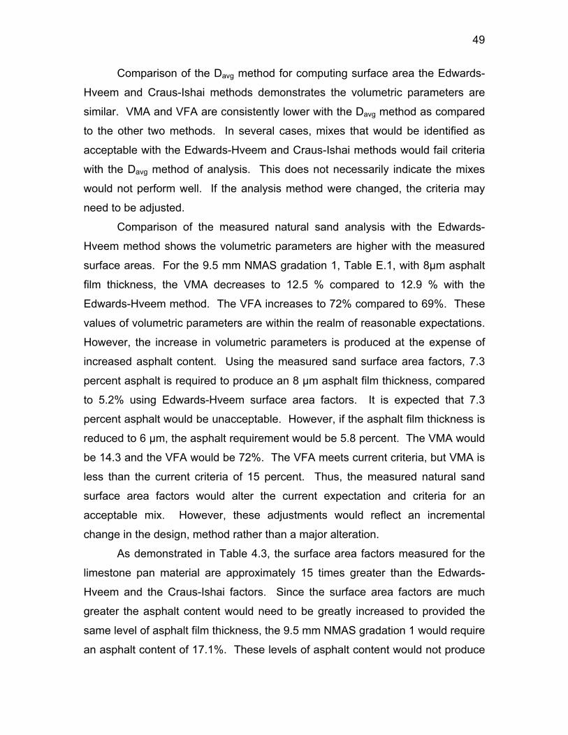
49

Comparison of the Davg method for computing surface area the Edwards-

Hveem and Craus-Ishai methods demonstrates the volumetric parameters are

similar. VMA and VFA are consistently lower with the Davg method as compared

to the other two methods. In several cases, mixes that would be identified as

acceptable with the Edwards-Hveem and Craus-Ishai methods would fail criteria

with the Davg method of analysis. This does not necessarily indicate the mixes

would not perform well. If the analysis method were changed, the criteria may

need to be adjusted.

Comparison of the measured natural sand analysis with the Edwards-

Hveem method shows the volumetric parameters are higher with the measured

surface areas. For the 9.5 mm NMAS gradation 1, Table E.1, with 8µm asphalt

film thickness, the VMA decreases to 12.5 % compared to 12.9 % with the

Edwards-Hveem method. The VFA increases to 72% compared to 69%. These

values of volumetric parameters are within the realm of reasonable expectations.

However, the increase in volumetric parameters is produced at the expense of

increased asphalt content. Using the measured sand surface area factors, 7.3

percent asphalt is required to produce an 8 µm asphalt film thickness, compared

to 5.2% using Edwards-Hveem surface area factors. It is expected that 7.3

percent asphalt would be unacceptable. However, if the asphalt film thickness is

reduced to 6 µm, the asphalt requirement would be 5.8 percent. The VMA would

be 14.3 and the VFA would be 72%. The VFA meets current criteria, but VMA is

less than the current criteria of 15 percent. Thus, the measured natural sand

surface area factors would alter the current expectation and criteria for an

acceptable mix. However, these adjustments would reflect an incremental

change in the design, method rather than a major alteration.

As demonstrated in Table 4.3, the surface area factors measured for the

limestone pan material are approximately 15 times greater than the Edwards-

Hveem and the Craus-Ishai factors. Since the surface area factors are much

greater the asphalt content would need to be greatly increased to provided the

same level of asphalt film thickness, the 9.5 mm NMAS gradation 1 would require

an asphalt content of 17.1%. These levels of asphalt content would not produce

50

workable mixes. Examination of Tables E.2 and E.5 indicates the asphalt film

thickness would need to be 2 µm in order for the volumetric parameters and the

asphalt content to reach reasonable levels. These comparison are demonstrated

in Figures 4.8 through 4.13.

Figure 4.8 shows the VMA for each of the analysis and the minimum VMA

required for the HMA mixture. All the cases meet the criteria, but further

evaluation of the percent binder needed shows that the values are unreasonable

for the measured the limestone.

Figure 4.9 shows that the measured limestone approach meets the

minimum VMA and using Table E.5 the percent binder needed is reasonable for

a film thickness of 2 µm.

Figure 4.10 shows the VFA values for the 19 mm nominal maximum size

gradation #1 assuming a film thickness of 8 µm. It also shows the VFA for the

same gradation for a film thickness of 2 µm using the specific surface area of the

measured limestone. The VFA value for a film thickness of 2 µm meets the

criteria using the specific gravity measured for the limestone material.

Figure 4.11 shows the VMA values for the four 19 mm nominal maximum

aggregate size gradation. Three of the gradation meets the criteria. Gradation

#4 does not meet the criteria by 0.5%, under this circumstance the mix could be

acceptable.

Figures 4.12 and 4.13 shows VFA and F/A ratio values, respectively, for

the four gradations with a 19mm nominal maximum size. They all meet the

criteria when it is assumed 2 µm for film thickness and the specific surface area

for the measured limestone is used for the calculation of the VFA.

It should be noted that the volumetric parameters are sensitive to the

compaction energy used to prepare samples. Marshall mix designs use two

levels of compaction energy, 50 and 75 blows per side for medium and heavy

traffic, respectively. The SuperPave gyratory compactor used to compact

SuperPave samples, increases compaction effort by increasing the number of

gyrations used for compaction. Mix designs for the high traffic roads use more

gyrations than designs for low volume loads. Increasing the compaction effort

51

FIGURE 4.8 VMA VALUES FOR 19 mm MIX #1 8µm FILM THICKNESS

VMA values for a film thickness of 8 microns

0.0%5.0%

10.0%15.0%20.0%25.0%30.0%35.0%40.0%

Methods

VMA

Edwards-Hveem

minimum VMA

Craus-IshaiDavg MethodMeasured SandMeasured Limestone

Craus-IshaiDavg MethodMeasured SandMeasured Limestone

FIGURE 4.9 VMA VALUES FOR 19 mm MIX #1 2 µm FILM THICKNESS

VMA values for a film thickness of 2 microns

0.0%2.0%

4.0%6.0%8.0%

10.0%12.0%

14.0%16.0%

Methods

VMA

Edwards-Hveem

minimum VMA

52

FIGURE 4.10 VFA VALUES FOR 19 mm NMAS #1

VFA values for 19 mm mix #1

0.0%10.0%20.0%30.0%40.0%50.0%60.0%70.0%80.0%90.0%

100.0%

Method

VFA

Edwards-Hveem

VFA (65% - 75%)

Craus-Ishai

Davg Method

Measured Sand

Measured Limestone

Measured Limestonewith FT = 2 microns

# 2# 3# 4

FIGURE 4.11 VMA FOR 19 mm NMAS GRADATIONS 2 µm FILM THICKNESS.

VMA for Limestone assuming FT = 2 microns

11.0%11.5%12.0%12.5%13.0%13.5%14.0%14.5%15.0%15.5%

VMA

# 1

minimum VMA

53

FIGURE 4.12 VFA FOR 19 mm NMAS GRADATIONS 2 µm. FILM THICKNESS

VFA for Limestone assuming FT = 2 microns

64.0%

66.0%

68.0%

70.0%

72.0%

74.0%

76.0%

VFA

# 1

VFA (65% -75%)

# 2

# 3

# 4

# 2

# 3

# 4

FIGURE 4.13 F/A FOR 19 mm NMAS GRADATIONS 2 µm. FILM THICKNESS

D/B for Limestone assuming FT = 2 microns

0.00

0.20

0.40

0.60

0.80

1.00

1.20

D/B

# 1

D/B (0.6 - 1.2)

54

has the effect of reducing the asphalt content needed to produce a certain level

of air voids. The effect of compaction effort is not considered in the volumetric

analysis based on aggregate surface area.

No data were collected during the research to evaluate how compaction

effort would affect the results of the surface area based volumetric analysis. It is

hypothesized that due to the angularity and the texture of the limestone, the

aggregate provides a structure that is significantly different than the structure

produced in a mix with natural sand. This structure would promote the

development of voids space between the aggregate, and the hence provide

VMA. These factors would not be captured in the volumetric analysis based on

the surface area of the aggregates.

EFFECT OF SURFACE AREA ON FILM THICKNESS

It is possible to determine the asphalt film thickness based on acceptable

parameters like VMA = 15.2 %, VTM = 4% and a percentage asphalt of 5%.

Figure 4.14 presents a 19 mm mix with surface areas for each of aggergate

sources and the Edwards-Hveem values. As expected, the computed film

thickness using the measured parameters for the limestone fines is much less

than the film thickness computed with the Edwards-Hveem surface area factors.

If the film thickness is actually 2 µm, as indicated on Figure 4.14, this would

indicate the mix should be very rut resistant, but may suffer fatigue and durability

problems.

EFFECT OF BAGHOUSE FINES

During asphalt concrete production, the aggregates are heated and dried

in a dryer drum. As the moisture content is reduce, the aggregates release dust

that is carried out of the drier and captured in baghouse filters. Since this

effectively removes dust from the aggregate, it has become common practice to

reintroduce a portion of the baghouse material into the asphalt concrete mix.

During mix design, no distinction is made between pan material collected by

sieving and the baghouse fines. These materials are treated as if their effect on

the mix is interchangeable. Comparison of Tables 4.2 and 4.3 demonstrates that

55

FIGURE 4.14 MEASURED SURFACE AREA VS. FILM THICKNESS FOR A

19mm MIX.

Specific Surface Area Vs Asphalt Film Thicknessfor VMA = 15.2%, VTM = 4%, Pb = 5%, 19mm mix

0

2

4

6

8

10

12

0 5 10 15 20 25 30 35 40

Surface Area m2/kg

Asp

halt

Film

Thi

ckne

ss ( µ

m)

Summersville

Beaver Boxley (A)

Beaver Boxley (B)

APAC Sand

Apac # 10

New Enterprise

Natural Sand

Edwards-Hveem

Edwards-Hveem

Natural Sand

Crushed limestone fines

baghouse fines have a much greater surface area than the sieve pan material.

The average surface area of the sieved pan material was 452 m2/kg and the

baghouse fine was 765 m2/kg.

Due to the greater surface area of the baghouse fines, introducing them

into the mix would require increasing the asphalt content in order to maintain a

given value of asphalt film thickness. As show in Figure 4.15, there is a

significant difference in the required binder content of the mix, when one percent

of baghouse material is introduced into the mix. The issue of replacing pan

material with baghouse fines has not been addressed in the literature.

SUMMARY OF DATA COLLECTION AND ANALYSIS

Examination of the traditional methods for computing asphalt film

thickness demonstrates several issues which indicate potential errors in the

process. The specific surface area factors attributed to Edwards cannot be

recreated from stated assumptions. Furthermore, the calculation of the total

56

FIGURE 4.15 EFFECT OF BAGHOUSE FINES USING GRADATION #1 NMAS

19 mm FOR A FILM THICKNESS OF 8 µm

0.0%

2.0%

4.0%

6.0%

8.0%

10.0%

12.0%

14.0%

16.0%

18.0%

20.0%

Methods

Perc

ent B

inde

r Pb

Edwards-Hveem

Edwards-Hveem with 1%baghouse

Craus-Ishai

Craus-Ishai with 1%baghouse

D method

D method with 1% baghousefine

Natural sand

Natural sand with 1%baghouse

Limestone

Limestone with 1% baghouse

surface area by multiplying a surface area factor, computed based on the

opening size of the sieve, by the total percent of material which passes the sieve,

is not logical. The Craus-Ishai approach to computing surface area is

reproducible. However, the conventional approach is to use these factors with

the cumulative percent passing each sieve.

An alternative method for computing surface area factors using the

average of the sieve sizes through which the aggregate passes and is retained

was developed. These surface area factors were multiplied by amount of

material retained on the sieve to determine the surface area. This approach is

more defensible than the Edwards-Hveem and Craus-Ishai methods.

Conventional methods of computing surface area of mixture use

computed surface area factors. The sole of information in the literature reporting

57

measured surface areas indicate measured surface area of fine materials are

greater than computed surface areas (Chapuis, 1992). This result was

supported by surface area measured during the research. It was found that the

measured surface area was approximately 15 times greater than the computed

surface area for limestone material finer than 0.075 mm.

Volumetric analysis using surface area factors derived from the literature

demonstrates that reasonable results can be produced. However, when the

measured values for the surface area are used, the creditability of the results are

at issue. The results produced with the measured natural sand specific surface

area are within the range of accepted mix design parameters, and the effect of

using these factors for mix design could be accommodated by adjusting the

volumetric criteria for mix design. However, the same cannot be said for the use

of the limestone surface area factors. The measured surface area of fine

limestone material is so much greater than the Edwards-Hveem factors that the

resulting volumetric analysis cannot reliably represent a realistic mix design.

The inability of the surface area method of volumetric analysis to produce

reasonable mix design results highlights the fact that the volumetric properties of

a compacted asphalt concrete mix are a function of the compaction effort used to

compact the mix. In addition to the surface area, aggregate texture and shape

affect compaction characteristics. This suggests the aggregate structure with in

the compacted mix must be considered during the volumetric analysis.

Finally, volumetric analysis considering the use of baghouse fines,

indicates these materials can have a different effect on the mix properties than

the simple replacement of the dust collected by sieving the aggregates. This

implies that if baghouse fines are introduced into a mix during production, then

this same quantity of baghouse fines should be included during the mix design.

58

CHAPTER 5 CONCLUSIONS AND RECOMMENDATIONS

CONCLUSIONS

Volumetric criteria for asphalt concrete mix design were derived based on

the work of McLeod in the 1950’s. These criteria are currently implemented in

both the Marshall and the SuperPave methods of mix design. Kandhal

researched the criteria and proposed the use of asphalt film thickness as

controlling factor in the mix design. However, McLeod and subsequent

researchers primarily focused on natural sand fine aggregate and used specific

surface area factors. These factors area based on an assumption that the

aggregate shape can be characterized as a sphere whose diameter is equal to

the length of the sides of the sieve opening.

The conventional method for computing aggregate surface area was

carefully evaluated and found to be flawed. An alternative method of using the

average dimension of the passing and the retaining sieve dimension, along with

the spherical assumption, was developed. Furthermore, it is believed that

multiplying the resulting volume by the percent material retained on a sieve

reasonably estimates the surface area of the aggregates greater than 0.15 mm.

The surface area of an aggregate blend is strongly dependent on the

characteristics and amount of material finer than 0.15 mm. Hence, the surface

area of these materials was measured using the Blaine air permeability

apparatus. If was found that natural sand has a somewhat greater surface area

than computed surface area. However, the measured surface area for limestone

fine materials is much greater than both the computed values and the measured

sand surface area.

The equations required for performing a volumetric analysis based on

surface area were derived from a phase diagram compared to the equations

derived by Kandhal et.al (1998-1). There is a dependency in the Kandhal

equations with respect to the treatment of absorbed binder. The derived

equations were programmed into a spreadsheet and a parametric study was

59

performed using different levels of asphalt film thickness and the aggregate

gradation.

Based on the evaluation and the analysis performed during this research,

several conclusions were developed, which are summarized as:

1. Need to properly account for absorbed binder to correctly compute

volumetric properties.

2. Using cumulative percent passing to compute surface area is not

accurate.

3. Edwards-Hveem surface area factor cannot be reconstructed from

stated assumptions.

4. The Craus-Ishai method for computing surface area factors is

reproducible.

5. The specific surface area of an aggregate gradation is dominated

by the percent of material passing the 0.15 mm sieve.

6. The surface area factors computed should be computed using the

average of the sieve opening for the passing and the retaining

sieve.

7. The surface area for a given aggregate gradation should be

computed using the percent material retained on each sieve, rather

than using the cumulative percent passing.

8. The measured surface area for the natural sand and the limestone

materials fines than 0.15 mm are significantly greater than the

Edwards-Hveem and the Craus-Ishai computed surface area

factors. The difference is much greater for the limestone than for

the natural sand. The measured values for the mineral filler from

natural sand is in reasonable agreement with the coefficient in the

Duriez-Arrambide equation. The minimum measured values for the

limestone mineral filler agreed with values measured by Chapuis

and Legare.

9. Volumetric analysis using the Edwards-Hveem and the Craus-Ishai

surface area factors produce reasonable results with respect to

60

expectations for mix design. This result is anticipated since mix

design criteria were developed from the Edwards-Hveem surface

area factors.

10. Volumetric analysis using the measured surface area factors for

natural sand and the limestone materials indicates the effective

asphalt content must be greater than is required using the

Edwards-Hveem surface area factors in order to maintain the

asphalt film thickness.

11. Based on the measured values for fine material surface area, if

asphalt content remains constant, mixes with limestone fine

material will have a much thinner asphalt film thickness than the

mixtures made with natural sands. This factor would indicate

limestone mixtures are more rut resistant but more fatigue

susceptible than natural sand mixtures.

12. The volumetric analysis method based on the surface area factors

ignores the effect of the aggregate shape and texture on the

compaction ability of the asphalt concrete mixture. Volumetric

parameters are dependent on the compaction effort placed on the

mixture. Volumetric analysis based on the surface area is not

capable of capturing this factor.

RECOMMENDATIONS

The volumetric analysis method based on aggregate surface area

presents an interesting approach for evaluating average asphalt film thickness.

However, it would be premature to suggest that asphalt film thickness should be

used as a mix design criteria. It is known that asphalt film thickness is directly

related to asphalt concrete performance with respect to thermal cracking, fatigue

cracking, and rutting. Thus, investigating the relationship between aggregate

type and surface area and resulting surface area has great potential in furthering

knowledge on the performance of asphalt concrete mixtures. Hence, the

recommendations from this research identify areas to refine the surface area

61

analysis method and the potential for using this information to improve asphalt

concrete performance.

1. There should be further evaluation of limestone fine material

surface area. For the materials evaluated during this research, a

wide range of surface areas were measured.

2. Further evaluation should be performed on production mix designs.

Average film thickness should be computed based on optimum

asphalt content, the gradation of the mix and measured surface

area of the material finer than 0.15 mm.

3. Research should be performed to relate asphalt film thickness to

parameters of pavement distress, including fatigue, thermal

cracking, and fatigue. The current findings indicate limestone

based materials may be superior to natural sands with respect to

rutting, but inferior with respect to fatigue and thermal cracking.

4. Due to the vast difference in the surface area between natural sand

and limestone, there may be a need to vary volumetric design

criteria as a function of the type of aggregate.

5. The surface area volumetric analysis does not capture the effect of

compaction effort on the volumetric properties of the mix. Hence,

implementation of this approach would required augmentation of

the analytical method with a methodology to capture the

compaction characteristics of the mix.

62

REFERENCE

1. Anderson, D.A., and J.P. Tarris, Adding Dust Collectors to Asphalt

Paving Mixtures, Transportation Research Board, Washington, D.C.,

Vol. 252. 1982.

2. Campen, J.F., J.R. Smith, L.G. Erickson, and L.R. Mertz, The

Relationship Between Voids, Surface Area, Film Thickness and

Stability in Bituminous Paving Mixtures, Proceedings, Association of

Asphalt Paving Technologists, Vol. 28, 1959.

3. Chapuis, R.P. and P. Legare, A Simple Method for Determination the

Surface Area of Fine Aggregates and Fillers in Bituminous Mixtures,

ASTM STP 1147, Philadelphia, PA, 1992

4. Craus, J., and I. Ishai, A Method for Determination of the Surface Area

of Fine Aggregates in Bituminous Mixtures, Journal of Testing and

Evaluation, Vol. 5., 1977.

5. Duriez, M., and J. Arrambide, Nouveau Traite de Materiaux de

Construction, Paris, 1962.

6. Federal Highway Administration. Status of the Nation's Highways,

Bridges, and Transit: 2002 Conditions and Performance Report.

http://www.fhwa.dot.gov/policy/2002cpr/ch1.htm. 02/27/2002

7. Harman, T., J. D’Angelo, and J. Bukowski, Federal Highway

Administration. SuperPave Asphalt Mixture Design. Workbook Version

5.1. Washington D.C. January 1999.

8. Kandhal, P.S., C.Y. Lynn, and F. Parker, Jr., Characterization Tests for

Mineral Fillers Related to Performance of Asphalt Paving Mixtures.

NCAT Report No.98-2. Auburn University, AL., January 1998.

9. Kandhal, P.S., K.Y. Foo, and R.B. Mallick. A Critical Review of VMA

Requirements in SuperPave. NCAT Report No.98-1. Auburn

University, AL., January 1998.

63

10. Kanneganti, V., Comparison of 19 mm SuperPave and Marshall Base

II Mixes in West Virginia, West Virginia University. Morgantown, WV.

2002

11. McLeod, N.W., Relationship Between Density, Bitumen Content, and

Voids Properties of Compacted Bituminous Paving Mixtures.

Proceedings, Highway Research Board, Volume 35, Washington, DC,

1956

12. McLeod, N.W., Voids Requirements for Dense-Graded Bituminous

Paving Mixtures. Special Technical Publication 252, ASTM,

Philadelphia, PA., 1959.

13. Roberts F.L., P.S. Kandhal, E.R. Brown, D. Lee, and T. W. Kennedy,

Hot Mix Asphalt Materials, Mixture Design, and Construction. Second

Edition, National Asphalt Pavement Association, Lanham, MD., 1996.

14. The Asphalt Institute, Mix Design Methods for Asphalt Concrete and

other Hot Mix Types, MS-2, Sixth Edition, 1993.

15. Tunnicliff, D.G., Biding Effects of Mineral Filler. Proceedings,

Association of Asphalt Paving Technologists, Vol. 36, 1967.

64

SPECIFICATIONS

1. West Virginia Division of Highways, Standard Specifications, 2000.

2. Standard Specification for SuperPave Volumetric Mix Design.

AASHTO Designation MP 2-99, 1999.

3. Guide to Designing Hot-Mix Asphalt using the Marshall Design

Method. WVDOT MP 402.02.22.2000.

4. Guide to Designing Hot-Mix Asphalt using the SuperPave Volumetric

Design System. WVDOT MP 402.02.28.2000.

5. Bulk Specific Gravity of Bituminous Paving Mixtures. AASHTO T166.

1993.

6. Maximum Specific Gravity of Bituminous Paving Mixtures. AASHTO

T209. 1994.

7. Determination of Specific Gravity and Absorption of Course Aggregate.

AASHTO T85. 1991.

8. Determination of Specific Gravity and Absorption of Fine Aggregate.

AASHTO T84. 1994.

9. Determination of Specific Gravity of Asphalt Cement. AASHTO 228.

1994.

10. Standard Test Method for Finesses of Hydraulic Cement by Air

Permeability Apparatus. ASTM C204. 1996

11. Standard Test Method for Density of Hydraulic Cement. ASTM C188.

1995

65

APPENDIX A SPECIFIC GRAVITY OF SAMPLES

TABLE A.1 SPECIFIC GRAVITIES OF THE FINE MATERIAL EVALUATED

Material A B C D Gsb GSa Ab%

APAC sample #1 2.684 2.780 1.29

APAC sample #2 2.603 2.692 1.28

Meadows Stone & Paving.

Sample (A)

499.6 658.9 976.3 504.7 2.667 2.742 1.02

Meadows Stone & Paving

Sample (B)

494.1 658.9 973.6 503.3 2.620 2.754 1.86

New Enterprise Stone &

lime

2.523

491.2 658.8 969.8 501.7 2.576 2.726 2.14 Southern W.V. Paving, Inc

489.7 658.8 969.1 500.5 2.575 2.730 2.21

490.2 658.8 965.0 500.5 2.523 2.664 2.10 Natural Sand

489.7 679.8 985.9 500.3 2.522 2.667 2.16

Where:

A = mass of oven dry sample in air, grams.

B = Mass of pycnometer filled to calibration mark with distilled water,

grams.

C = Mass of pycnometer, sample and water to calibration, grams.

D = Mass saturated-surface-dry sample in air, grams.

Gsb = Bulk specific gravity.

Gsa = Apparent specific gravity.

%Ab. = Percent absorption.

66

TABLE A.2 SPECIFIC GRAVITIES OF THE BAGHOUSE MATERIAL

EVALUATED

Material A B Gsb Average Gsb

56.097 20.7 2.710

55.461 20.5 2.705 APAC sample 1

56.014 20.7 2.706

2.707

53.893 20.8 2.591

53.713 20.9 2.570 J.F. Allen Company

54.684 21.0 2.604

2.588

52.925 19.8 2.673

52.560 19.7 2.668 Meadows Stone & Paving, Sample (A)

52.698 19.7 2.675

2.672

56.035 20.8 2.694

53.480 19.8 2.701 Meadows Stone & Paving, Sample (B)

55.186 20.7 2.666

2.687

56.826 21.0 2.706

55.432 20.5 2.704 New Enterprise Stone & lime

56.326 20.8 2.708

2.706

55.610 20.4 2.726

56.259 20.6 2.731 Tri-State Asphalt Company

56.027 20.5 2.733

2.730

56.448 21.0 2.688

54.835 20.4 2.688 West Virginia Paving, Inc

55.249 20.6 2.682

2.686

54.782 20.2 2.712

54.200 20.0 2.710 Gasaway

51.314 18.9 2.715

2.712

54.520 20.0 2.726

53.351 19.6 2.722 Southern W.V. Paving, Inc (Summersville)

51.219 18.9 2.710

2.723

67

Where:

A = Mass of oven-dry sample in air, grams

B = Volume displaced, cm3.

Gsb = Bulk specific gravity.

68

APPENDIX B SURFACE AREA FOR THE MATERIAL PASS 0.15MM AND RETAINED ON 0.075MM

TABLE B.1 APAC SAMPLE # 2 SURFACE AREA FOR THE MATERIAL PASS

0.15 mm AND RETAINED ON 0.075 mm.

Source:Type:TestedD ate: 2/27/2002

S s = 396.6 bs = 0.9

ρ s = 3.15 εs = 0.5

T s = 136.16 1.858

24 2.603

Porosity # 1 # 2 # 3 # 4 # 5 # 60.513 3.53 3.55 3.56 3.56 3.55 3.530.500 3.87 3.90 3.87 3.90 3.83 3.870.488 4.25 4.21 4.26 4.31 4.25 4.180.475 4.56 4.63 4.68 4.68 4.70 4.63

Porosity T S0.513 3.55 0.691 18.4520.500 3.87 0.696 18.4490.488 4.24 0.701 18.4590.475 4.65 0.706 18.448 b = 2.255

0.9996 > 0.997

APAC sam ple #2Lim estone

Constant

Volum e Sam ple =

Tem perature = S . G . (ov en Dry Sam ple) =

T im eW eight of Sam ple

2.3582.4182.4792.539

2.539C orrelation Coeff ic ient =

W eight of Sam ple 2.3582.4182.479

T3ε

0.47

0.475

0.48

0.485

0.49

0.495

0.5

0.505

0.51

0.515

0.69 0.692 0.694 0.696 0.698 0.7 0.702 0.704 0.706 0.708

Bed

Por

osity

69

TABLE B.2 APAC SAMPLE #1 SURFACE AREA FOR THE MATERIAL PASS


Source:Type:TestedDate: 3/1/2002

Ss = 396.6 bs = 0.9

ρs = 3.15 εs = 0.5

Ts = 136.16 1.858

24 2.684

Porosity # 1 # 2 # 3 # 4 # 5 # 60.5 3.03 3.04 3.07 3.04 3.06 3.03

0.488 3.39 3.38 3.35 3.35 3.28 3.350.475 3.74 3.77 3.74 3.76 3.73 3.730.463 4.15 4.13 4.15 4.16 4.13 4.18

Porosity T S0.500 3.05 0.617 30.7130.488 3.35 0.624 30.6560.475 3.75 0.634 30.6920.463 4.15 0.642 30.697 b = 1.407

0.9990 > 0.997

APAC sample #1Limestone

Constant

Volume Sample =

Temperature = S. G. (oven Dry Sample) =

TimeWeight of Sample

2.4932.5532.6182.678

2.678Correlation Coefficient =

Weight of Sample 2.4932.5532.618

T3ε

0.46

0.465

0.47

0.475

0.48

0.485

0.49

0.495

0.5

0.505

0.615 0.62 0.625 0.63 0.635 0.64 0.645

Bed

Por

osity

70

TABLE B.3 SUMMERSVILLE LIMESTONE SURFACE AREA FOR THE

MATERIAL PASS 0.15 mm AND RETAINED ON 0.075 mm.


Ss = 396.6 bs = 0.9

ρs = 3.15 εs = 0.5

Ts = 136.16 1.858

24 2.575

Porosity # 1 # 2 # 3 # 4 # 5 # 60.470 3.78 3.75 3.81 3.74 3.77 3.730.455 4.21 4.28 4.31 4.26 4.21 4.240.440 4.96 4.81 4.75 4.83 4.87 4.760.430 5.28 5.27 5.24 5.22 5.24 5.23

Porosity T S0.470 3.76 0.625 24.8420.455 4.25 0.633 24.8360.440 4.83 0.641 24.8620.430 5.25 0.646 24.829 b = 1.654

0.9992 > 0.997

SummervilleLimestone

Constant

Volume Sample =



2.5362.6072.6792.727

2.727Correlation Coefficient =


T3ε

0.425

0.430

0.435

0.440

0.445

0.450

0.455

0.460

0.465

0.470

0.475

0.620 0.625 0.630 0.635 0.640 0.645 0.650

Bed

Por

osity

71

TABLE B.4 BEAVER BOXLEY (A) SURFACE AREA FOR THE MATERIAL

PASS 0.15 mm AND RETAINED ON 0.075 mm.


Ss = 396.6 bs = 0.9

ρs = 3.15 εs = 0.5

Ts = 136.16 1.858

24 2.667

Porosity # 1 # 2 # 3 # 4 # 5 # 60.500 2.31 2.28 2.37 2.06 2.22 2.270.485 2.84 2.87 2.78 2.21 2.21 2.340.470 3.03 3.00 3.15 2.68 2.65 2.710.455 3.09 3.28 3.37 3.12 3.32 3.20

Porosity T S0.500 2.25 0.531 21.4650.485 2.54 0.538 21.5000.470 2.87 0.546 21.5110.455 3.23 0.552 21.457 b = 1.623

0.9974 > 0.9972.701

Correlation Coefficient =


2.4782.5522.6262.701



Beaver Boxley (A)Limestone

Constant

Volume Sample =

T3ε

0.450

0.455

0.460

0.465

0.470

0.475

0.480

0.485

0.490

0.495

0.500

0.505

0.525 0.530 0.535 0.540 0.545 0.550 0.555

Bed

Por

osity

72

TABLE B.5 BEAVER BOXLEY (B) SURFACE AREA FOR THE MATERIAL

PASS 0.15 mm AND RETAINED ON 0.075 mm.


Ss = 396.6 bs = 0.9

ρs = 3.15 εs = 0.5

Ts = 136.16 1.858

24 2.620

Porosity # 1 # 2 # 3 # 4 # 5 # 60.513 2.53 3.65 3.56 3.56 3.65 3.600.500 2.87 3.90 3.93 3.90 3.93 3.870.488 3.25 4.21 4.26 4.21 4.25 4.240.475 3.56 4.53 4.68 4.68 4.70 4.53

Porosity T S0.513 3.43 0.679 13.8990.500 3.73 0.683 13.9070.488 4.07 0.687 13.9030.475 4.45 0.690 13.900 b = 2.771

0.9994 > 0.9972.556



2.3732.4342.4952.556



Beaver Boxley (B)Limestone

Constant

Volume Sample =

T3ε

0.47

0.475

0.48

0.485

0.49

0.495

0.5

0.505

0.51

0.515

0.678 0.68 0.682 0.684 0.686 0.688 0.69 0.692

Bed

Por

osity

73

TABLE B.6 NEW ENTERPRISE SURFACE AREA FOR THE MATERIAL PASS



Ss = 396.6 bs = 0.9

ρs = 3.15 εs = 0.5

Ts = 136.16 1.858

24 2.523

Porosity # 1 # 2 # 3 # 4 # 5 # 60.500 3.18 3.00 3.12 3.06 3.15 3.150.488 3.35 3.34 3.34 3.35 3.41 3.430.475 3.71 3.75 3.64 3.71 3.65 3.710.463 3.96 4.09 4.03 4.00 4.03 4.03

Porosity T S0.500 3.11 0.623 11.1820.488 3.37 0.626 11.1730.475 3.70 0.629 11.1810.463 4.02 0.632 11.178 b = 3.177

0.9983 > 0.9972.517



2.3442.4002.4612.517



New EnterpriseLimestone

Constant

Volume Sample =

T3ε

0.460

0.465

0.470

0.475

0.480

0.485

0.490

0.495

0.500

0.505

0.623 0.624 0.625 0.626 0.627 0.628 0.629 0.630 0.631 0.632 0.633

Bed

Por

osity

74

TABLE B.7 NATURAL SAND SURFACE AREA FOR THE MATERIAL PASS



Ss = 396.6 bs = 0.9

ρs = 3.15 εs = 0.5

Ts = 136.16 1.858

24 2.522

Porosity # 1 # 2 # 3 # 4 # 5 # 60.475 1.96 2.00 1.84 2.00 2.00 1.870.462 2.09 2.09 2.11 2.13 2.14 2.210.450 2.30 2.37 2.30 2.34 2.31 2.330.437 2.50 2.50 2.66 2.50 2.63 2.53

Porosity T S0.475 1.95 0.457 7.2590.462 2.13 0.459 7.2630.450 2.33 0.460 7.2590.437 2.55 0.462 7.260 b = 3.496

0.9987 > 0.9972.636



2.4602.5192.5772.636



Natural Sand

Constant

Volume Sample =

T3ε

0.435

0.44

0.445

0.45

0.455

0.46

0.465

0.47

0.475

0.48

0.456 0.457 0.458 0.459 0.46 0.461 0.462 0.463

Bed

Por

osity

75

APPENDIX C SURFACE AREA PAN MATERIAL

TABLE C.1 SUMMERSVILLE PAN MATERIAL SURFACE AREA


Ss = 396.6 bs = 0.9

ρs = 3.15 εs = 0.5

Ts = 136.16 1.858

24 2.575

Porosity # 1 # 2 # 30.530 69.78 69.76 69.560.500 99.65 98.71 100.000.470 143.06 143.25 143.170.440 195.00 195.28 195.56

Porosity T S0.530 69.70 3.221 456.0500.500 99.45 3.526 457.8310.470 143.16 3.855 462.3220.440 195.28 4.079 454.349 b = 0.862

0.9970 > 0.9972.679


W eight of Sample 2.2492.3922.536

2.2492.3922.5362.679


TimeW eight of Sample

SummersvilleLimestone

Constant

Volume Sample =

T3ε

0

0.1

0.2

0.3

0.4

0.5

0.6

0 0.5 1 1.5 2 2.5 3 3.5 4 4.5

Bed

Por

osity

76

TABLE C.2 BEAVER BOXLEY SAMPLE (A) PAN MATERIAL SURFACE AREA


Ss = 396.6 bs = 0.9

ρs = 3.15 εs = 0.5

Ts = 136.16 1.858

24 2.62

Porosity # 1 # 2 # 30.530 36.35 36.43 36.300.500 54.75 54.12 54.530.470 79.05 79.04 79.120.440 118.75 118.50 118.93

Porosity T S0.530 36.36 2.327 435.5840.500 54.47 2.609 435.5850.470 79.07 2.865 431.5570.440 118.73 3.180 436.355 b = 0.777

0.9992 > 0.9972.726



2.2882.4342.5802.726



Beaver Boxley (A)Limestone

Constant

Volume Sample =

T3ε

0

0.2

0.4

0.6

0.8

1

1.2

0 0.2 0.4 0.6 0.8 1 1.2

Bed

Por

osity

T3ε

0

0.1

0.2

0.3

0.4

0.5

0.6

0 0.5 1 1.5 2 2.5 3

Bed

Por

osity

77

TABLE C.3 BEAVER BOXLEY SAMPLE (B) PAN MATERIAL SURFACE AREA


Ss = 396.6 bs = 0.9

ρs = 3.15 εs = 0.5

Ts = 136.16 1.858

24 2.667

Porosity # 1 # 2 # 30.530 25..22 25.43 24.970.500 34.56 34.39 34.530.470 50.00 50.00 50.000.440 40.00 90.00 90.00

Porosity T S0.530 25.20 1.937 292.6480.500 34.49 2.076 285.2600.470 50.00 2.278 286.9640.440 73.33 2.499 290.615 b = 0.831

0.9951 > 0.9972.775



2.3292.4782.6262.775



Beaver Boxley (B)Limestone

Constant

Volume Sample =

T3ε

0.000

0.100

0.200

0.300

0.400

0.500

0.600

0.000 0.500 1.000 1.500 2.000 2.500 3.000

Bed

Por

osity

T3ε

0.000

0.100

0.200

0.300

0.400

0.500

0.600

0.000 0.500 1.000 1.500 2.000 2.500 3.000

Bed

Por

osity

78

TABLE C.4 APAC SAMPLE #1PAN MATERIAL SURFACE AREA


Ss = 396.6 bs = 0.9

ρs = 3.15 εs = 0.5

Ts = 136.16 1.858

24 2.603

Porosity # 1 # 2 # 30.530 67.87 67.81 67.930.500 95.18 97.00 97.180.470 137.00 134.15 135.680.440 190.18 190.75 189.46

Porosity T S0.530 67.87 3.179 436.3410.500 96.45 3.472 437.8850.470 135.61 3.752 437.6150.440 190.13 4.024 436.535 b = 0.869

0.9999 > 0.9972.708



2.2732.4182.5632.708




Constant

Volume Sample =

T3ε

0

0.1

0.2

0.3

0.4

0.5

0.6

0 0.5 1 1.5 2 2.5 3 3.5 4 4.5

Bed

Por

osity

79

TABLE C.5 APAC SAMPLE #2 PAN MATERIAL SURFACE AREA


Ss = 396.6 bs = 0.9

ρs = 3.15 εs = 0.5

Ts = 136.16 1.858

24 2.684

Porosity # 1 # 2 # 30.530 145.92 145.46 145.370.500 194.31 193.96 194.750.470 266.14 264.15 264.270.440 369.15 368.43 369.03

Porosity T S0.530 145.58 4.656 480.4380.500 194.34 4.929 475.9800.470 264.85 5.244 475.8610.440 368.87 5.606 479.742 b = 0.967

0.9981 > 0.9972.793



2.3442.4932.6432.793




Constant

Volume Sample =

T3ε

0

0.1

0.2

0.3

0.4

0.5

0.6

0 1 2 3 4 5 6

Bed

Por

osity

80

TABLE C.6 NEW ENTERPRISE PAN MATERIAL SURFACE AREA Source:Type:TestedDate: 3/13/2002

Ss = 396.6 bs = 0.9

ρs = 3.15 εs = 0.5

Ts = 136.16 1.858

24 2.523

Porosity # 1 # 2 # 30.530 25.50 25.62 26.370.500 39.53 39.87 37.150.470 71.84 73.21 72.250.440 108.34 108.21 107.56

Porosity T S0.530 25.83 1.961 630.8340.500 38.85 2.204 590.2550.470 72.43 2.742 629.2110.440 108.04 3.034 608.773 b = 0.679

0.9893 > 0.9972.625



2.2032.3442.4842.625



New EnterpriseLimestone

Constant

Volume Sample =

T3ε

0

0.1

0.2

0.3

0.4

0.5

0.6

0 0.5 1 1.5 2 2.5 3 3.5

Bed

Por

osity

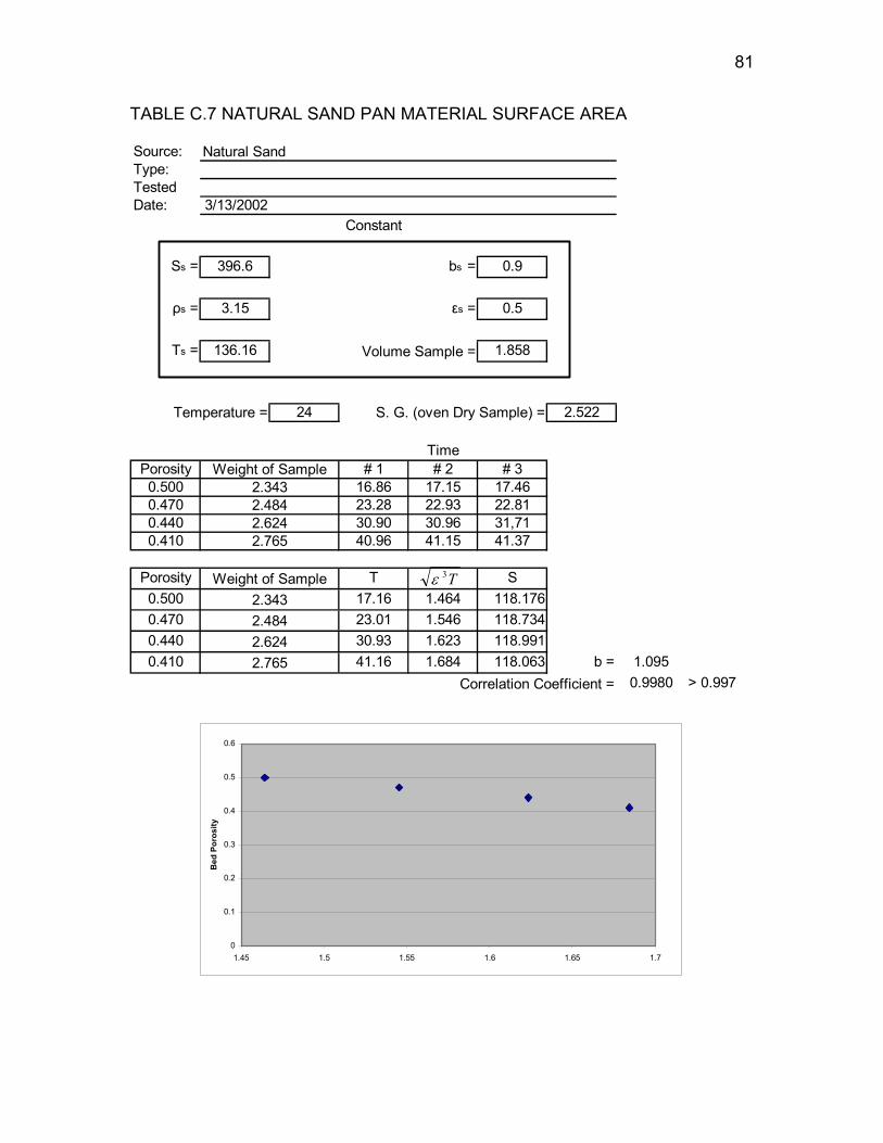
81

TABLE C.7 NATURAL SAND PAN MATERIAL SURFACE AREA


Ss = 396.6 bs = 0.9

ρs = 3.15 εs = 0.5

Ts = 136.16 1.858

24 2.522

Porosity # 1 # 2 # 30.500 16.86 17.15 17.460.470 23.28 22.93 22.810.440 30.90 30.96 31,710.410 40.96 41.15 41.37

Porosity T S0.500 17.16 1.464 118.1760.470 23.01 1.546 118.7340.440 30.93 1.623 118.9910.410 41.16 1.684 118.063 b = 1.095

0.9980 > 0.9972.765



2.3432.4842.6242.765



Natural Sand

Constant

Volume Sample =

T3ε

0

0.1

0.2

0.3

0.4

0.5

0.6

1.45 1.5 1.55 1.6 1.65 1.7

Bed

Por

osity

82

APPENDIX D BAGHOUSE FINES SPECIFIC SURFACE AREAS

TABLE D.1 SUMMERSVILLE BAGHOUSE FINES SPECIFIC SURFACE AREA


Ss = 396.6 bs = 0.9

ρs = 3.15 εs = 0.5

Ts = 136.16 1.858

24 2.575

Porosity # 1 # 2 # 30.530 69.78 69.76 69.560.500 99.65 98.71 100.000.470 143.06 143.25 143.170.440 195.00 195.28 195.56

Porosity T S0.530 69.70 3.221 456.0500.500 99.45 3.526 457.8310.470 143.16 3.855 462.3220.440 195.28 4.079 454.349 b = 0.862

0.9970 > 0.9972.679


W eight of Sample 2.2492.3922.536

2.2492.3922.5362.679


TimeW eight of Sample

SummersvilleLimestone

Constant

Volume Sample =

T3ε

0

0.1

0.2

0.3

0.4

0.5

0.6

0 0.5 1 1.5 2 2.5 3 3.5 4 4.5

Bed

Por

osity

83

TABLE D.2 GASAWAY BAGHOUSE FINES SPECIFIC SURFACE AREA.


Ss = 396.6 bs = 0.9

ρs = 3.15 εs = 0.5

Ts = 136.16 1.858

24 2.712

Porosity # 1 # 2 # 30.530 81.75 85.78 81.400.500 118.03 117.71 115.810.470 172.62 173.03 170.530.440 255.06 256.21 254.18

Porosity T S0.530 82.98 3.515 579.5580.500 117.18 3.828 568.2970.470 172.06 4.228 570.8120.440 255.15 4.661 576.705 b = 0.801

0.9976 > 0.9972.822



2.3682.5192.6702.822



GasawayBaghouse Fines

Constant

Volume Sample =

T3ε

0

0.1

0.2

0.3

0.4

0.5

0.6

0 0.5 1 1.5 2 2.5 3 3.5 4 4.5 5

Bed

Por

osity

84

TABLE D.3 BEAVER BOXLEY BAGHOUSE FINE SAMPLE (A) SPECIFIC

SURFACE AREA


Ss = 396.6 bs = 0.9

ρs = 3.15 εs = 0.5

Ts = 136.16 1.858

24 2.672

Porosity # 1 # 2 # 30.530 457.81 446.81 464.650.500 664.90 680.50 667.430.470 935.37 947.03 942.340.440 1334.23 1328.46 1330.35

Porosity T S0.530 456.42 8.245 1196.0680.500 670.94 9.160 1212.3190.470 941.58 9.889 1203.3760.440 1331.01 10.649 1199.306 b = 0.843

0.9987 > 0.9972.780


Beaver Boxley sample (A)


2.3332.4822.6312.780



Baghouse Fines

Constant

Volume Sample =

T3ε

0

0.1

0.2

0.3

0.4

0.5

0.6

0 2 4 6 8 10 12

Bed

Por

osity

85

TABLE D.4 BEAVER BOXLEY BAGHOUSE FINES SAMPLE (B) SPECIFIC

SURFACE AREA


Ss = 396.6 bs = 0.9

ρs = 3.15 εs = 0.5

Ts = 136.16 1.858

24 2.687

Porosity # 1 # 2 # 30.533 234.20 216.28 226.240.503 326.87 312.40 320.640.473 496.53 431.87 463.300.443 640.18 631.43 636.81

Porosity T S0.533 225.57 5.839 823.1370.503 319.97 6.378 822.3800.473 463.90 7.007 832.3320.443 636.14 7.441 819.451 b = 0.852

0.9977 > 0.9972.780



2.3332.4822.6312.780



Beaver Boxley sample (B)Baghouse Fines

Constant

Volume Sample =

T3ε

0

0.1

0.2

0.3

0.4

0.5

0.6

0 1 2 3 4 5 6 7 8

Bed

Por

osity

86

TABLE D.5 APAC BAGHOUSE FINE SPECIFIC SURFACE AREA


Ss = 396.6 bs = 0.9

ρs = 3.15 εs = 0.5

Ts = 136.16 1.858

24 2.707

Porosity # 1 # 2 # 30.560 194.62 191.62 187.430.530 272.34 269.31 268.400.500 378.37 370.37 382.280.480 458.56 458.34 450.45

Porosity T S0.560 191.22 5.795 743.0150.530 270.02 6.340 748.4920.500 377.01 6.864 750.8800.480 455.78 7.101 740.844 b = 0.909

0.9973 > 0.9972.615



2.2132.3642.5152.615



APAC sample #1Baghouse Fines

Constant

Volume Sample =

T3ε

0.47

0.48

0.49

0.5

0.51

0.52

0.53

0.54

0.55

0.56

0.57

0 1 2 3 4 5 6 7 8

Bed

Por

osity

87

TABLE D.6 J.F. ALLEN BAGHOUSE FINES SPECIFIC SURFACE AREA


Ss = 396.6 bs = 0.9

ρs = 3.15 εs = 0.5

Ts = 136.16 1.858

24 2.588

Porosity # 1 # 2 # 30.540 180.99 181.62 181.790.508 271.20 271.31 271.160.477 374.96 375.39 374.800.456 470.87 471.34 471.09

Porosity T S0.540 181.47 5.342 741.5030.508 271.22 5.969 757.9850.477 375.05 6.379 746.4430.456 471.10 6.687 743.798 b = 0.877

0.9952 > 0.9972.615



2.2132.3642.5152.615



JFABaghouse Fines

Constant

Volume Sample =

T3ε

0.45

0.46

0.47

0.48

0.49

0.5

0.51

0.52

0.53

0.54

0.55

0 1 2 3 4 5 6 7 8

Bed

Por

osity

88

TABLE D.7 NEW ENTERPRISE BAGHOUSE FINES SPECIFIC SURFACE

AREA


Ss = 396.6 bs = 0.9

ρs = 3.15 εs = 0.5

Ts = 136.16 1.858

24 2.706

Porosity # 1 # 2 # 30.562 74.81 75.28 70,050.534 99.68 104.78 104.060.506 140.56 136.59 145.580.478 196.96 191.50 195.23

Porosity T S0.562 75.05 3.646 511.5240.534 102.84 3.955 510.2960.506 140.91 4.269 509.6750.478 194.56 4.605 511.523 b = 0.881

0.9998 > 0.9972.626



2.2042.3442.4852.626



New EnterpriseBaghouse Fines

Constant

Volume Sample =

T3ε

0.47

0.48

0.49

0.5

0.51

0.52

0.53

0.54

0.55

0.56

0.57

0 0.5 1 1.5 2 2.5 3 3.5 4 4.5 5

Bed

Por

osity

89

TABLE D.8 W.V. PAVING BAGHOUSE FINES SPECIFIC SURFACE AREA


Ss = 396.6 bs = 0.9

ρs = 3.15 εs = 0.5

Ts = 136.16 1.858

24 2.686

Porosity # 1 # 2 # 30.530 112.34 119.31 119.590.500 163.06 165.55 161.370.470 242.53 235.34 232.780.440 335.34 345.65 344.12

Porosity T S0.530 117.08 4.175 622.9700.500 163.33 4.518 613.3280.470 236.88 4.959 617.4150.440 341.70 5.395 620.311 b = 0.832

0.9984 > 0.9972.795



2.3462.4952.6452.795



W.V. PavingBaghouse Fines

Constant

Volume Sample =

T3ε

0.000

0.100

0.200

0.300

0.400

0.500

0.600

0.000 1.000 2.000 3.000 4.000 5.000 6.000

Bed

Por

osity

T3ε

0.000

0.100

0.200

0.300

0.400

0.500

0.600

0.000 1.000 2.000 3.000 4.000 5.000 6.000

Bed

Por

osity

90

TABLE D.9 TRI-STATE BAGHOUSE FINES SPECIFIC SURFACE AREA


Ss = 396.6 bs = 0.9

ρs = 3.15 εs = 0.5

Ts = 136.16 1.858

24 2.730

Porosity # 1 # 2 # 30.530 122.34 129.31 129.590.500 173.06 165.21 171.370.470 242.53 235.34 232.780.440 343.18 355.59 353.12

Porosity T S0.530 127.08 4.350 566.5330.500 169.88 4.609 551.7300.470 236.88 4.957 548.7940.440 350.63 5.463 562.756 b = 0.871

0.9888 > 0.9972.841



2.3842.5362.6892.841



Tri-StateBaghouse Fines

Constant

Volume Sample =

T3ε

0.000

0.100

0.200

0.300

0.400

0.500

0.600

0.000 1.000 2.000 3.000 4.000 5.000 6.000

Bed

Por

osity

91

APPENDIX E VOLUMETRIC ANALYSIS RESULTS

TABLE E.1 VOLUMETRIC ANALYSIS FOR 9.5 mm GRADATION #1

Film Thickness 10

µm

Edwards-Hveem Craus-Ishai Davg

method Measured

Sand Measured Limestone

Film Thickness 8

µm


method Measured


Wbe 0.052534 0.060043 0.050215 0.082161 0.260319 Wbe 0.042027 0.048034 0.040172 0.065729 0.208255 Wb 0.065313 0.072822 0.062994 0.094940 0.273098 Wb 0.054806 0.060813 0.052951 0.078508 0.221034 Vba 0.012528 0.012528 0.012528 0.012528 0.012528 Vba 0.012528 0.012528 0.012528 0.012528 0.012528 Vbe 0.051504 0.058866 0.049231 0.080550 0.255214 Vbe 0.041203 0.047093 0.039385 0.064440 0.204172 Vb 0.064032 0.071394 0.061759 0.093079 0.267743 Vb 0.053731 0.059621 0.051913 0.076969 0.216700

Wm 1.065313 1.072822 1.062994 1.094940 1.273098 Wm 1.054806 1.060813 1.052951 1.078508 1.221034 Pb 6.1% 6.8% 5.9% 8.7% 21.5% Pb 5.2% 5.7% 5.0% 7.3% 18.1%

Pbe 4.9% 5.6% 4.7% 7.5% 20.4% Pbe 4.0% 4.5% 3.8% 6.1% 17.1% Vsb 0.404040 0.404040 0.404040 0.404040 0.404040 Vsb 0.404040 0.404040 0.404040 0.404040 0.404040

Vmm 0.455544 0.462906 0.453271 0.484591 0.659255 Vmm 0.445243 0.451133 0.443425 0.468481 0.608212 Vmb 0.474525 0.482194 0.472157 0.504782 0.686724 Vmb 0.463795 0.469930 0.461901 0.488001 0.633554 VMA 14.9% 16.2% 14.4% 20.0% 41.2% VMA 12.9% 14.0% 12.5% 17.2% 36.2% D/B 0.90 1.02 0.86 1.36 3.72 D/B 0.72 0.82 0.69 1.11 3.10 VFA 73% 75% 72% 80% 90% VFA 69% 71% 68% 77% 89%

% Vbe 11% 12% 10% 16% 37% % Vbe 9% 10% 9% 13% 32% % Vb 13% 15% 13% 18% 39% % Vb 12% 13% 11% 16% 34%

Film

Thickness 6 µm


method Measured


Film Thickness 4

µm


method Measured



Wm 1.044299 1.048805 1.042908 1.062076 1.168970 Wm 1.033792 1.036796 1.032865 1.045643 1.116906 Pb 4.2% 4.7% 4.1% 5.8% 14.5% Pb 3.3% 3.5% 3.2% 4.4% 10.5%

Pbe 3.0% 3.4% 2.9% 4.6% 13.4% Pbe 2.0% 2.3% 1.9% 3.1% 9.3% Vsb 0.404040 0.404040 0.404040 0.404040 0.404040 Vsb 0.404040 0.404040 0.404040 0.404040 0.404040


% Vbe 7% 8% 7% 10% 26% % Vbe 5% 5% 4% 7% 19% % Vb 10% 10% 9% 13% 29% % Vb 7% 8% 7% 10% 22%

Film

Thickness 2 µm


method Measured


Wbe 0.010507 0.012009 0.010043 0.016432 0.052064 Wb 0.023286 0.024788 0.022822 0.029211 0.064843 Vba 0.012528 0.012528 0.012528 0.012528 0.012528 Vbe 0.010301 0.011773 0.009846 0.016110 0.051043 Vb 0.022829 0.024302 0.022375 0.028638 0.063571

Wm 1.023286 1.024788 1.022822 1.029211 1.064843 Pb 2.3% 2.4% 2.2% 2.8% 6.1%

Pbe 1.0% 1.2% 1.0% 1.6% 4.9% Vsb 0.404040 0.404040 0.404040 0.404040 0.404040

Vmm 0.414341 0.415814 0.413887 0.420150 0.455083 Vmb 0.431605 0.433139 0.431132 0.437657 0.474045 VMA 6.4% 6.7% 6.3% 7.7% 14.8% D/B 0.19 0.21 0.18 0.29 0.89 VFA 37% 40% 36% 48% 73%

% Vbe 2% 3% 2% 4% 11% % Vb 5% 6% 5% 7% 13%

92


Film Thickness 10

µm


method Measured


Film Thickness 8

µm

Edwards-Hveem

Davg method

Measured Sand

Measured Limestone

Wbe 0.049902 0.057071 0.047235 0.073987 0.238480 Wbe 0.039922 0.037788 0.059189 0.190784 Wb 0.062081 0.069250

Craus-Ishai

0.045657 0.059414 0.086165 0.250658 Wb 0.052100 0.057836 0.049967 0.071368 0.202962

Vba 0.011940 0.011940 0.011940 0.011940 0.011940 Vba 0.011940 0.011940 0.011940 0.011940 0.011940 Vbe 0.048924 0.055952 0.046309 0.072536 Vbe 0.039139 0.044762 0.037047 0.058029 0.187043 Vb 0.060864 0.067892 0.058249 0.084476 0.245743 Vb 0.051079 0.056702 0.048987 0.069968 0.198983

Wm 1.062081 1.069250 1.059414 1.086165 1.250658 Wm 1.052100 1.057836 1.049967 1.071368 1.202962 Pb 5.8% 6.5% 5.6% 7.9% 20.0% Pb 5.0% 5.5% 4.8% 6.7% 16.9%

Pbe 4.7% 5.3% 4.5% 6.8% 19.1% Pbe 3.8% 4.3% 3.6% 5.5% 15.9% Vsb 0.385060 0.385060 0.385060 0.385060 0.385060 Vsb 0.385060 0.385060 0.385060 0.385060 0.385060


% Vbe 11% 12% 10% 15% 36% % Vbe 9% 10% 8% 13% 31% % Vb 13% 15% 13% 18% 38% % Vb 12% 13% 11% 15% 33%

Film

Thickness 6 µm


method Measured


Film Thickness 4

µm


method Measured



Wm 1.042120 1.046421 1.040520 1.056571 1.155266 Wm 1.032140 1.035007 1.031073 1.041773 1.107570 Pb 4.0% 4.4% 3.9% 5.4% 13.4% Pb 3.1% 3.4% 3.0% 4.0% 9.7%

Pbe 2.9% 3.3% 2.7% 4.2% 12.4% Pbe 1.9% 2.2% 1.8% 2.8% 8.6% Vsb 0.385060 0.385060 0.385060 0.385060 0.385060 Vsb 0.385060 0.385060 0.385060 0.385060 0.385060


% Vbe 7% 8% 6% 10% 26% % Vbe 5% 5% 4% 7% 19% % Vb 10% 10% 9% 12% 28% % Vb 7% 8% 7% 9% 21%

Film

Thickness 2 µm


method Measured


Wbe 0.009980 0.011414 0.009447 0.014797 0.047696 Wb 0.022159 0.023593 0.021626 0.026976 0.059875 Vba 0.011940 0.011940 0.011940 0.011940 0.011940 Vbe 0.009785 0.011190 0.009262 0.014507 0.046761 Vb 0.021725 0.023130 0.021202 0.026447 0.058701

Wm 1.022159 1.023593 1.021626 1.026976 1.059875 Pb 2.2% 2.3% 2.1% 2.6% 5.6%

Pbe 1.0% 1.1% 0.9% 1.4% 4.5% Vsb 0.385060 0.385060 0.385060 0.385060 0.385060

Vmm 0.394844 0.396250 0.394322 0.399567 0.431820 Vmb 0.411296 0.412761 0.410752 0.416215 0.449813 VMA 6.4% 6.7% 6.3% 7.5% 14.4% D/B 0.20 0.22 0.18 0.29 0.90 VFA 37% 40% 36% 47% 72%

% Vbe 2% 3% 2% 3% 10% % Vb 5% 6% 5% 6% 13%

0.233803

93


Film Thickness 10

µm


method Measured


Film Thickness 8

µm


method Measured



Wm 1.057376 1.064454 1.054475 1.077009 1.215113 Wm 1.048281 1.053944 1.045961 1.063988 1.174471 Pb 5.4% 6.1% 5.2% 7.2% 17.7% Pb 4.6% 5.1% 4.4% 6.0% 14.9%

Pbe 4.3% 4.9% 4.0% 6.0% 16.7% Pbe 3.5% 4.0% 3.3% 4.9% 13.8% Vsb 0.376364 0.376364 0.376364 0.376364 0.376364 Vsb 0.376364 0.376364 0.376364 0.376364 0.376364


% Vbe 10% 12% 10% 14% 33% % Vbe 8% 9% 8% 11% 29% % Vb 13% 14% 12% 16% 35% % Vb 11% 12% 11% 14% 31%

Film Thickness 6

µm


method Measured


Film Thickness 4

µm


method Measured



Wm 1.039187 1.043434 1.037446 1.050967 1.133829 Wm 1.030092 1.032924 1.028932 1.037946 1.093187 Pb 3.8% 4.2% 3.6% 4.8% 11.8% Pb 2.9% 3.2% 2.8% 3.7% 8.5%

Pbe 2.6% 3.0% 2.5% 3.7% 10.8% Pbe 1.8% 2.0% 1.7% 2.5% 7.4% Vsb 0.376364 0.376364 0.376364 0.376364 0.376364 Vsb 0.376364 0.376364 0.376364 0.376364 0.376364


% Vbe 6% 7% 6% 9% 23% % Vbe 4% 5% 4% 6% 17% % Vb 9% 10% 9% 12% 25% % Vb 7% 8% 7% 9% 19%

Film Thickness 2

µm


method Measured


Wbe 0.009094 0.010510 0.008514 0.013021 0.040642 Wb 0.020998 0.022414 0.020418 0.024925 0.052546 Vba 0.011670 0.011670 0.011670 0.011670 0.011670 Vbe 0.008916 0.010304 0.008347 0.012766 0.039845 Vb 0.020586 0.021974 0.020017 0.024436 0.051515

Wm 1.020998 1.022414 1.020418 1.024925 1.052546 Pb 2.1% 2.2% 2.0% 2.4% 5.0%

Pbe 0.9% 1.0% 0.8% 1.3% 3.9% Vsb 0.376364 0.376364 0.376364 0.376364 0.376364

Vmm 0.385280 0.386668 0.384712 0.389130 0.416209 Vmb 0.401334 0.402780 0.400741 0.405344 0.433551 VMA 6.2% 6.6% 6.1% 7.1% 13.2% D/B 0.21 0.24 0.20 0.30 0.92 VFA 36% 39% 34% 44% 70%

% Vbe 2% 3% 2% 3% 9% % Vb 5% 5% 5% 6% 12%

94


Film Thickness 10

µm


method Measured


Film Thickness 8

µm


method Measured



Wm 1.063492 1.070969 1.060763 1.088763 1.255757 Wm 1.053236 1.059217 1.051053 1.073453 1.207048 Pb 6.0% 6.6% 5.7% 8.2% 20.4% Pb 5.1% 5.6% 4.9% 6.8% 17.2%

Pbe 4.8% 5.5% 4.6% 7.0% 19.4% Pbe 3.9% 4.4% 3.7% 5.7% 16.1% Vsb 0.386100 0.386100 0.386100 0.386100 0.386100 Vsb 0.386100 0.386100 0.386100 0.386100 0.386100


% Vbe 11% 12% 11% 16% 37% % Vbe 9% 10% 9% 13% 32% % Vb 14% 15% 13% 18% 39% % Vb 12% 13% 11% 15% 34%

Film Thickness 6

µm


method Measured


Film Thickness 4

µm


method Measured



Wm 1.042980 1.047466 1.041342 1.058142 1.158339 Wm 1.032724 1.035714 1.031632 1.042832 1.109630 Pb 4.1% 4.5% 4.0% 5.5% 13.7% Pb 3.2% 3.4% 3.1% 4.1% 9.9%

Pbe 3.0% 3.4% 2.8% 4.3% 12.6% Pbe 2.0% 2.3% 1.9% 2.9% 8.8% Vsb 0.386100 0.386100 0.386100 0.386100 0.386100 Vsb 0.386100 0.386100 0.386100 0.386100 0.386100


% Vbe 7% 8% 7% 10% 26% % Vbe 5% 5% 5% 7% 19% % Vb 10% 11% 9% 13% 28% % Vb 8% 8% 7% 10% 21%

Film Thickness 2

µm


method Measured


Wbe 0.010256 0.011751 0.009710 0.015310 0.048709 Wb 0.022468 0.023963 0.021922 0.027522 0.060921 Vba 0.011972 0.011972 0.011972 0.011972 0.011972 Vbe 0.010055 0.011521 0.009520 0.015010 0.047754 Vb 0.022027 0.023493 0.021492 0.026982 0.059726

Wm 1.022468 1.023963 1.021922 1.027522 1.060921 Pb 2.2% 2.3% 2.1% 2.7% 5.7%

Pbe 1.0% 1.1% 1.0% 1.5% 4.6% Vsb 0.386100 0.386100 0.386100 0.386100 0.386100

Vmm 0.396155 0.397621 0.395620 0.401110 0.433854 Vmb 0.412662 0.414189 0.412104 0.417823 0.451932 VMA 6.4% 6.8% 6.3% 7.6% 14.6% D/B 0.20 0.23 0.19 0.29 0.90 VFA 38% 41% 37% 47% 73%

% Vbe 2% 3% 2% 4% 11% % Vb 5% 6% 5% 6% 13%

95

TABLE E.5 VOLUMETRIC ANALYSIS FOR 19 mm GRADATION #1

Film Thickness 10

µm


method Measured


Film Thickness 8

µm


method Measured Limestone

Wbe 0.055490 0.062938 0.051425 0.075814 0.242918 Wbe 0.044392 0.050350 0.041140 0.194334 Wb 0.067204 0.074652 0.063139 0.087528 0.254632 Wb 0.056106 0.062064 0.052854 0.206048 Vba 0.011484 0.011484 0.011484 0.011484 0.011484 Vba 0.011484 0.011484 0.011484 0.011484 Vbe 0.054402 0.061704 0.050417 0.074328 0.238155 Vbe 0.043522 0.049363 0.040334 0.190524 Vb 0.065886 0.073188 0.061901 0.085812 0.249639 Vb 0.055006 0.060848 0.051818 0.202008

Wm 1.067204 1.074652 1.063139 1.087528 1.254632 Wm 1.056106 1.062064 1.052854 1.206048 Pb 6.3% 6.9% 5.9% 8.0% 20.3% Pb 5.3% 5.8% 5.0% 17.1%

Pbe 5.2% 5.9% 4.8% 7.0% 19.4% Pbe 4.2% 4.7% 3.9% 16.1% Vsb 0.370370 0.370370 0.370370 0.370370 0.370370 Vsb 0.370370 0.370370 0.370370 0.370370

Vmm 0.424772 0.432074 0.420787 0.444698 0.608525 Vmm 0.413892 0.419734 0.410704 0.560894 Vmb 0.442471 0.450077 0.438320 0.463227 0.633881 Vmb 0.431138 0.437222 0.427817 0.584265 VMA 16.3% 17.7% 15.5% 20.0% 41.6% VMA 14.1% 15.3% 13.4% 36.6% D/B 1.04 1.17 0.97 1.39 3.87 D/B 0.84 0.95 0.78 3.22 VFA 75% 77% 74% 80% 90% VFA 72% 74% 70% 89%

% Vbe 12% 14% 12% 16% 38% % Vbe 10% 11% 9% 33% % Vb 15% 16% 14% 19% 39% % Vb 13% 14% 12% 35%

Film

Thickness 6 µm


method Measured


Film Thickness 4

µm


method Measured Limestone

Wbe 0.033294 0.037763 0.030855 0.045489 0.145751 Wbe 0.022196 0.025175 0.020570 0.097167 Wb 0.045008 0.049477 0.042569 0.057203 0.157465 Wb 0.033910 0.036889 0.032284 0.108881 Vba 0.011484 0.011484 0.011484 0.011484 0.011484

Measured Sand

0.060651 0.072366 0.011484 0.059462 0.070947 1.072366

6.7% 5.7%

0.370370 0.429833 0.447742

17.3% 1.13 77% 13% 16%

Measured Sand

0.030326 0.042040

Vba 0.011484 0.011484 0.011484 0.011484 0.011484 Vbe 0.032641 0.037022 0.030250 0.044597 0.142893 Vbe 0.021761 0.024682 0.020167 0.029731 0.095262 Vb 0.044126 0.048507 0.041735 0.056081 0.154377 Vb 0.033245 0.031651 0.041215 0.106746

Wm 1.045008 1.049477 1.042569 1.057203 1.157465 Wm 1.033910 1.036889 1.032284 1.042040 1.108881 Pb 4.3% 4.7% 4.1% 5.4% 13.6% Pb 3.3% 3.6% 3.1% 4.0% 9.8%

Pbe 3.2% 3.6% 3.0% 4.3% 12.6% Pbe 2.1% 2.4% 2.0% 2.9% 8.8% Vsb 0.370370 0.370370 0.370370 0.370370 0.370370 Vsb 0.370370 0.370370 0.370370 0.370370 0.370370


% Vbe 8% 9% 7% 10% 27% % Vbe 5% 6% 5% 7% 20% % Vb 11% 11% 10% 13% 29% % Vb 8% 9% 8% 10% 22%

Film

Thickness 2 mm


method Measured


Wbe 0.011098 0.012588 0.010285 0.015163 0.048584 Wb 0.022812 0.024302 0.021999 0.026877 0.060298 Vba 0.011484 0.011484 0.011484 0.011484 0.011484 Vbe 0.010880 0.012341 0.010083 0.014866 0.047631 Vb 0.022365 0.023825 0.021568 0.026350 0.059115

Wm 1.022812 1.024302 1.021999 1.026877 1.060298 Pb 2.2% 2.4% 2.2% 2.6% 5.7%

Pbe 1.1% 1.2% 1.0% 1.5% 4.6% Vsb 0.370370 0.370370 0.370370 0.370370 0.370370

Vmm 0.381251 0.382711 0.380454 0.385236 0.418001 Vmb 0.397136 0.398657 0.396306 0.401287 0.435418 VMA 6.7% 7.1% 6.5% 7.7% 14.9% D/B 0.22 0.25 0.20 0.30 0.92 VFA 41% 44% 39% 48% 73%

% Vbe 3% 3% 3% 4% 11% % Vb 6% 6% 5% 7% 14%

0.036166

96


Film Thickness 10

µm


method Measured


Film Thickness 8

µm


method Measured



Wm 1.075074 1.085215 1.068192 1.077467 1.222463 Wm 1.062429 1.070541 1.056922 1.064343 1.180340 Pb 7.0% 7.9% 6.4% 7.2% 18.2% Pb 5.9% 6.6% 5.4% 6.0% 15.3%

Pbe 5.9% 6.8% 5.3% 6.1% 17.2% Pbe 4.8% 5.5% 4.3% 4.9% 14.3% Vsb 0.374532 0.374532 0.374532 0.374532 0.374532 Vsb 0.374532 0.374532 0.374532 0.374532 0.374532


% Vbe 14% 15% 12% 14% 34% % Vbe 11% 13% 10% 12% 29% % Vb 16% 18% 15% 17% 36% % Vb 14% 15% 13% 14% 31%

Film

Thickness 6 µm


method Measured


Film Thickness 4

µm


method Measured



Wm 1.049783 1.055867 1.045653 1.051219 1.138216 Wm 1.037137 1.041193 1.034384 1.038094 1.096093 Pb 4.7% 5.3% 4.4% 4.9% 12.1% Pb 3.6% 4.0% 3.3% 3.7% 8.8%

Pbe 3.6% 4.2% 3.2% 3.7% 11.1% Pbe 2.4% 2.8% 2.2% 2.5% 7.7% Vsb 0.374532 0.374532 0.374532 0.374532 0.374532 Vsb 0.374532 0.374532 0.374532 0.374532 0.374532


% Vbe 9% 10% 8% 9% 24% % Vbe 6% 7% 5% 6% 17% % Vb 11% 13% 11% 12% 26% % Vb 9% 10% 8% 9% 20%

Film

Thickness 2 mm


method Measured


Wbe 0.012646 0.014674 0.011269 0.013124 0.042124 Wb 0.024491 0.026519 0.023115 0.024970 0.053969 Vba 0.011613 0.011613 0.011613 0.011613 0.011613 Vbe 0.012398 0.014386 0.011048 0.012867 0.041298 Vb 0.024011 0.025999 0.022662 0.024480 0.052911

Wm 1.024491 1.026519 1.023115 1.024970 1.053969 Pb 2.4% 2.6% 2.3% 2.4% 5.1%

Pbe 1.2% 1.4% 1.1% 1.3% 4.0% Vsb 0.374532 0.374532 0.374532 0.374532 0.374532

Vmm 0.386930 0.388918 0.385580 0.387399 0.415829 Vmb 0.403052 0.405123 0.401646 0.403540 0.433156 VMA 7.1% 7.6% 6.8% 7.2% 13.5% D/B 0.31 0.36 0.28 0.32 1.00 VFA 43% 47% 41% 44% 70%

% Vbe 3% 4% 3% 3% 10% % Vb 6% 6% 6% 6% 12%

97


Film Thickness 10

µm


method Measured


Film Thickness 8

µm


method Measured


Wbe 0.042878 0.047598 0.232255 Wbe 0.038078 0.041176 0.069502 0.034302 0.032941 0.055602 0.185804 0.054996 0.059716 0.053294 0.081620 0.244373 Wb 0.046420 0.045059 0.067720 0.197922

Vba 0.011880 0.011880 0.011880 0.011880 0.011880 Vba 0.011880 0.011880 0.011880 0.011880 0.011880 Vbe 0.042037 0.046664 0.040369 0.068139 0.227701 Vbe 0.033630 0.037331 0.032295 0.054512 0.182161 Vb 0.053917 0.058545 0.052249 0.080020 0.239581 Vb 0.045510 0.049212 0.044176 0.066392 0.194041

Wm 1.054996 1.059716 1.053294 1.081620 1.244373 Wm 1.046420 1.050196 1.045059 1.067720 1.197922 Pb 5.2% 5.6% 5.1% 7.5% 19.6% Pb 4.4% 4.8% 4.3% 6.3% 16.5%

Pbe 4.1% 4.5% 3.9% 6.4% 18.7% Pbe 3.3% 3.6% 3.2% 5.2% 15.5% Vsb 0.383142 0.383142 0.383142 0.383142 0.383142 Vsb 0.383142 0.383142 0.383142 0.383142 0.383142


% Vbe 9% 10% 9% 14% 36% % Vbe 8% 9% 7% 12% 31% % Vb 12% 10% 13% 12% 17% 38% % Vb 10% 11% 15% 33%


method Measured


Film Thickness 4

µm

Davg method

Measured Sand

Measured Limestone


Wm 1.037845 1.040677 1.036824 1.053819 1.151471 Wm 1.029269 1.031157 1.028589 1.039919 1.105020 Pb 3.6% 3.9% 3.0% 3.6% 5.1% 13.2% Pb 2.8% 2.8% 3.8% 9.5%

Pbe 2.5% 2.7% 2.4% 4.0% 12.1% Pbe 1.7% 1.8% 1.6% 2.7% 8.4% Vsb 0.383142 0.383142 0.383142 0.383142 0.383142 Vsb 0.383142 0.383142 0.383142 0.383142 0.383142

Vmm 0.408364 0.411140 0.407363 0.424025 0.519762 Vmm 0.399957 0.401807 0.399289 0.410398 0.474222 Vmb 0.425379 0.428271 0.424337 0.441693 0.541419 Vmb 0.416621 0.418549 0.415926 0.427497 0.493981 VMA 9.9% 10.5% 9.7% 13.3% 29.2% VMA 8.0% 8.5% 7.9% 10.4% 22.4% D/B 0.50 0.55 0.37 0.48 0.79 2.42 D/B 0.33 0.32 0.53 1.68 VFA 60% 62% 59% 70% 86% VFA 50% 53% 49% 61% 82%

% Vbe 6% 7% 6% 9% 25% % Vbe 4% 4% 4% 6% 18% % Vb 9% 9% 9% 12% 27% % Vb 7% 7% 7% 9% 21%

Film

Thickness 2 µm


method Measured


Wbe 0.008576 0.009520 0.008235 0.013900 0.046451 Wb 0.020694 0.021637 0.020353 0.026018 0.058569 Vba 0.011880 0.011880 0.011880 0.011880 0.011880 Vbe 0.008407 0.009333 0.008074 0.013628 0.045540 Vb 0.020288 0.021213 0.019954 0.025508 0.057421

Wm 1.020694 1.021637 1.020353 1.026018 1.058569 Pb 2.0% 2.1% 2.0% 2.5% 5.5%

Pbe 0.8% 0.9% 0.8% 1.4% 4.4% Vsb 0.383142 0.383142 0.383142 0.383142 0.383142

Vmm 0.391549 0.392475 0.391216 0.396770 0.428682 Vmb 0.407864 0.408828 0.407516 0.413302 0.446544 VMA 6.1% 6.3% 6.0% 7.3% 14.2% D/B 0.17 0.19 0.16 0.27 0.88 VFA 34% 36% 33% 45% 72%

% Vbe 2% 2% 2% 3% 10% % Vb 5% 5% 5% 6% 13%

Wb 0.050196

Film Thickness 6

µm

Edwards-Hveem Craus-Ishai

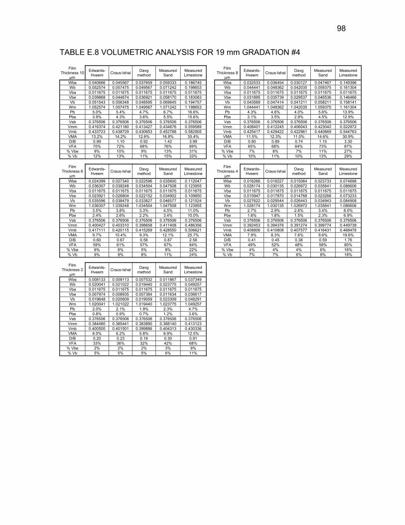
98


Film Thickness 10

µm


method Measured


Film Thickness 8

µm


method Measured


Wbe 0.040666 0.045567 0.037659 0.030127 0.059333 0.186745 Wbe 0.032533 0.036454 0.047467 0.149396 Wb 0.052574 0.057475 0.049567 0.071242 0.198653

0.011675 0.011675 0.011675 0.011675 0.011675 Vba 0.011675 0.011675 0.011675 0.011675 Vbe 0.039868 0.044674 0.036921 0.058170 0.183083 Vbe 0.031895 0.035739 0.029537 0.046536 0.146466 Vb 0.051543 0.056348 0.048595 0.069845 0.194757 Vb 0.043569 0.047414 0.041211 0.058211 0.158141

Wm 1.052574 1.057475 1.049567 1.071242 1.198653 Wm 1.044441 1.048362 1.042035 1.059375 1.161304 Pb 5.0% 5.4% 4.7% 6.7% 16.6% Pb 4.3% 4.6% 4.0% 5.6% 13.9%

Pbe 3.9% 4.3% 3.6% 5.5% 15.6% Pbe 3.1% 3.5% 2.9% 4.5% 12.9% Vsb 0.376506 0.376506 0.376506 0.376506 0.376506 Vsb 0.376506 0.376506 0.376506 0.376506 0.376506


% Vbe 9% 10% 9% 13% 31% % Vbe 7% 8% 7% 11% 27% % Vb 12% 13% 11% 15% 33% % Vb 10% 11% 10% 13% 29%

Film

Thickness 6 µm


method Measured


Film Thickness 4

µm


method Measured



Wm 1.036307 1.039248 1.034504 1.047508 1.123955 Wm 1.028174 1.030135 1.026972 1.035641 1.086606 Pb 3.5% 3.8% 3.3% 4.5% 11.0% Pb 2.7% 2.9% 2.6% 3.4% 8.0%

Pbe 2.4% 2.6% 2.2% 3.4% 10.0% Pbe 1.6% 1.8% 1.5% 2.3% 6.9% Vsb 0.376506 0.376506 0.376506 0.376506 0.376506 Vsb 0.376506 0.376506 0.376506 0.376506 0.376506


% Vbe 6% 6% 5% 8% 22% % Vbe 4% 4% 4% 6% 16% % Vb 9% 9% 8% 11% 24% % Vb 7% 7% 6% 8% 18%

Film

Thickness 2 µm


method

Measured Sand

Measured Limestone

0.009113 0.007532 0.011867 0.037349 Wb 0.020041 0.021022 0.019440 0.023775 0.049257 Vba 0.011675 0.011675 0.011675 0.011675 0.011675 Vbe 0.007974 0.008935 0.007384 0.011634 0.036617 Vb 0.019648 0.020609 0.019059 0.023309 0.048291

Wm 1.020041 1.021022 1.019440 1.023775 1.049257 Pb 2.0% 2.1% 1.9% 2.3% 4.7%

Pbe 0.8% 0.9% 0.7% 1.2% 3.6% Vsb 0.376506 0.376506 0.376506 0.376506 0.376506

Vmm 0.384480 0.385441 0.383890 0.388140 0.413123 Vmb 0.400500 0.401501 0.399886 0.404313 0.430336 VMA 6.0% 6.2% 5.8% 6.9% 12.5% D/B 0.20 0.23 0.19 0.30 0.91 VFA 33% 36% 32% 42% 68%

% Vbe 2% 2% 2% 3% 9% % Vb 5% 5% 5% 6% 11%

Wb 0.044441 0.048362 0.042035 0.059375 0.161304 Vba 0.011675

Wbe 0.008133

Evaluation of the effect of fines on asphalt concrete

Documents

Transcript of Evaluation of the effect of fines on asphalt concrete