Evaluation of Ten Psychometric Criteria for Circumplex ...€¦ · Evaluation of Ten Psychometric...

Methods of Psychological Research Online 2004, Vol. 9, No. 1 Fachbereich Psychologie

Internet: http://www.mpr-online.de © 2004 Universität Koblenz-Landau

Evaluation of Ten Psychometric Criteria for Circumplex

Structure

G. Scott Acton William Revelle

Rochester Institute of Technology Northwestern University

This study tested for sensitivity to circumplex structure in six existing and four new

psychometric criteria that assess the circumplex properties of interstitiality, equal

spacing, constant radius, and no preferred rotation. Simulations showed one criterion

to be sensitive to equal versus unequal axes (Fisher Test) and four to be sensitive to

interstitiality versus simple structure (Gap Test, Variance Test 2, Rotation Test, and

Minkowski Test). Five criteria were ineffective (Squared Loadings Index, Gap* Test,

Gap Difference Test, Cosine Difference Test, and Variance Test 1). Deviation scoring

improved the effectiveness of most criteria and is thus recommended for assessing cir-

cumplex structure. This study provides new and effective means for discovering com-

plex interrelations of variables where they exist. The circumplex, which falls in the

middle of a hierarchy of models in degree of parsimony, may most accurately reflect a

complex domain.

Keywords: circumplex, simple structure, simulation, factor analysis

A common model for representing psychological data is simple structure (Thurstone,

1947). According to one common interpretation, data are simple structured when items

or scales have non-zero factor loadings on one and only one factor (Revelle & Rocklin,

1979)1. Despite the commonplace application of simple structure, some psychological

models are defined by a lack of simple structure. Circumplexes (Guttman, 1954) are one

kind of model in which simple structure is lacking.

G. Scott Acton, Department of Psychology, Rochester Institute of Technology, Rochester, USA;

William Revelle, Department of Psychology, Northwestern University, Evanston, USA.

Correspondence concerning this article should be addressed to G. Scott Acton, Department of Psy-

chology, Rochester Institute of Technology, 92 Lomb Memorial Drive, Rochester, NY 14623-5604, USA.

Phone: (585) 475-2422. E-mail: [email protected].

1 This interpretation actually defines a special case of Thurstonian simple structure called independent

cluster structure.

2 MPR-Online 2004, Vol. 9, No. 1

A number of elementary requirements can be teased out of the idea of circumplex

structure. First, circumplex structure implies minimally that variables are interrelated;

random noise does not a circumplex make. Second, circumplex structure implies that

the domain in question is optimally represented by two and only two dimensions. Third,

circumplex structure implies that variables do not group or clump along the two axes,

as in simple structure, but rather that there are always interstitial variables between

any orthogonal pair of axes (Saucier, 1992). In the ideal case, this quality will be re-

flected in equal spacing of variables along the circumference of the circle (Gurtman,

1994; Wiggins, Steiger, & Gaelick, 1981). Fourth, circumplex structure implies that

variables have a constant radius from the center of the circle, which implies that all

variables have equal communality on the two circumplex dimensions (Fisher, 1997;

Gurtman, 1994). Fifth, circumplex structure implies that all rotations are equally good

representations of the domain (Conte & Plutchik, 1981; Larsen & Diener, 1992).

Circumplex models have been applied to such diverse variables as cognitive abilities

(Guttman, 1954); color perception (Shepard, 1962); vocational interests (Tracey &

Rounds, 1993); affective states (Yik, Russell, & Feldman Barrett, 1999); interpersonal

traits, problems, and goals (Acton & Revelle, 2002; Alden, Wiggins, & Pincus, 1990;

Dryer & Horowitz, 1997; Gurtman & Pincus, 2000); interpersonal values (Locke, 2000);

interpersonal interactions (Markey, Funder, & Ozer, 2003; Wagner, Kiesler, & Schmidt,

1995); social comparison (Locke, 2003); social support (Trobst, 2000); family relation-

ships (Schaefer, 1997); personality disorders (Soldz, Budman, Demby, & Merry, 1993);

adjectives in English and German (Saucier, Ostendorf, & Peabody, 2001); and the Big

Five personality factors (Hofstee, de Raad, & Goldberg, 1992; Johnson & Ostendorf,

1993). Although a review of circumplex models applied to all of these areas is beyond

the scope of this article, a recent book provides broad coverage of this domain (Plutchik

& Conte, 1997). The most common method for assessing circumplex structure has been

the "eyeball test"—variables are plotted in two-dimensional space using their factor

loadings as coordinates and are said to comprise a circumplex if they appear to form a

circle. This method has intuitive appeal but is rather unsystematic.

To bring greater rigor to bear on the question of circumplex structure, a number of

authors have developed criteria that purportedly assess various circumplex properties.

Joining the ranks of these authors, we present herein four new criteria that we devel-

oped to assess a relatively neglected circumplex property, lack of preferred rotation. In

addition, we review six existing criteria that assess the circumplex properties of intersti-

Acton & Revelle: Evaluation of Ten Circumplex Criteria 3

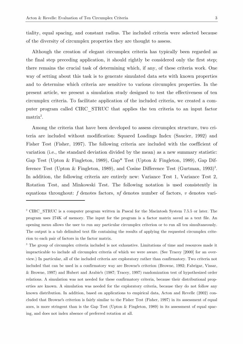
tiality, equal spacing, and constant radius. The included criteria were selected because

of the diversity of circumplex properties they are thought to assess.

Although the creation of elegant circumplex criteria has typically been regarded as

the final step preceding application, it should rightly be considered only the first step;

there remains the crucial task of determining which, if any, of these criteria work. One

way of setting about this task is to generate simulated data sets with known properties

and to determine which criteria are sensitive to various circumplex properties. In the

present article, we present a simulation study designed to test the effectiveness of ten

circumplex criteria. To facilitate application of the included criteria, we created a com-

puter program called CIRC_STRUC that applies the ten criteria to an input factor

matrix2.

Among the criteria that have been developed to assess circumplex structure, two cri-

teria are included without modification: Squared Loadings Index (Saucier, 1992) and

Fisher Test (Fisher, 1997). The following criteria are included with the coefficient of

variation (i.e., the standard deviation divided by the mean) as a new summary statistic:

Gap Test (Upton & Fingleton, 1989), Gap* Test (Upton & Fingleton, 1989), Gap Dif-

ference Test (Upton & Fingleton, 1989), and Cosine Difference Test (Gurtman, 1993)3.

In addition, the following criteria are entirely new: Variance Test 1, Variance Test 2,

Rotation Test, and Minkowski Test. The following notation is used consistently in

equations throughout: f denotes factors, nf denotes number of factors, v denotes vari-

2 CIRC_STRUC is a computer program written in Pascal for the Macintosh System 7.5.5 or later. The

program uses 274K of memory. The input for the program is a factor matrix saved as a text file. An

opening menu allows the user to run any particular circumplex criterion or to run all ten simultaneously.

The output is a tab delimited text file containing the results of applying the requested circumplex crite-

rion to each pair of factors in the factor matrix. 3 The group of circumplex criteria included is not exhaustive. Limitations of time and resources made it

impracticable to include all circumplex criteria of which we were aware. (See Tracey [2000] for an over-

view.) In particular, all of the included criteria are exploratory rather than confirmatory. Two criteria not

included that can be used in a confirmatory way are Browne's criterion (Browne, 1992; Fabrigar, Vissar,

& Browne, 1997) and Hubert and Arabie's (1987; Tracey, 1997) randomization test of hypothesized order

relations. A simulation was not needed for these confirmatory criteria, because their distributional prop-

erties are known. A simulation was needed for the exploratory criteria, because they do not follow any

known distribution. In addition, based on applications to empirical data, Acton and Revelle (2002) con-

cluded that Browne's criterion is fairly similar to the Fisher Test (Fisher, 1997) in its assessment of equal

axes, is more stringent than is the Gap Test (Upton & Fingleton, 1989) in its assessment of equal spac-

ing, and does not index absence of preferred rotation at all.


ables, nv denotes number of variables4, θ denotes angles of rotation, θv denotes the angu-

lar position of a variable v on the circumplex, R denotes Minkowski R, φfv denotes the

factor loading on factor f and variable v, and φfvθ denotes the factor loading on factor f

and variable v and angle of rotation θ.

Interstitiality

The Squared Loadings Index (SQLI; Saucier, 1992) is an index of interstitiality—that

is, the degree to which variables fall in between any orthogonal pair of axes. A circum-

plex should have many interstitial variables, whereas a simple structure should have

few. The formula for SQLI is

SQLIfv =

∑

∑

=

=

φ−φ

φ+φ

nv

vvv

nv

vvv

1

222

21

1

222

21

)(

)( (1)

Equal Spacing

In a circumplex, variables should be uniformly distributed around the circle. This

implies that they should be equally spaced. Equal spacing can be assessed in two ways:

first, by calculating the angular difference of observed variables from each other; second,

by calculating the angular difference of observed variables from the location where e-

qually spaced variables should be.

Observed gaps. One index of equal spacing is that the distance between adjacent

variables (the gaps; Upton & Fingleton, 1989) should have minimal variance. A gap is

the distance from one variable to the next (so long as one is consistent for all variables,

it does not matter whether the next variable is in a clockwise or counterclockwise direc-

4 Note that, in the simulations that follow, nf was constrained to equal 2, in keeping with the definition of

a circumplex. Some models, however (e.g., the abridged Big Five circumplex), contain more than two

factors, thus justifying the present notation. Note also that all of the criteria imply that the center of the

circumplex is identical to the point of origin of the coordinate system formed by the two factors making

up the circumplex. This implies a correlation of -1 between variables at 180-degree angles from one an-

other. Although this type of circumplex is the most commonly encountered, particularly in research on

personality or emotions, it is not the only possible one. For example, correlations between variables could

as well range from 0 to 1, particularly when there is a general factor, such as in research on cognitive

abilities.


tion). The Gap Test, also called Distance to Next, is defined as the variance of the gaps.

The equation for the Gap Test is

Gap Test = σXv

2, (2)

where Xv = (θv+1 – θv) for v = 1 to (nv – 1), and Xv = (2π + θ1 – θnv) for v = nv.

Because gaps differ in size, an alternative index of gaps (Gap*; Upton & Fingleton,

1989) has been developed; it is the minimum gap on either side of a variable. The Gap*

Test, also called Nearest Neighbor, is the maximum of these minima (Gaps*). The equa-

tion for the Gap* Test is

Gap* Test = max[min(θv – θv-1, θv+1 – θv)] (3)

for v = 2 to (nv – 1), and max[min(θnv – θnv-1, 2π + θ1 – θnv)] for v = nv.

Ideal gaps. The Gap Difference Test (GDIFF Test), also called Distance to Ideal, re-

quires the calculation of the gap between a variable and the location where an equally

spaced variable should be (Upton & Fingleton, 1989). This Gap Difference (GDIFF) is

calculated as the difference in radians between actual and ideal angles. The GDIFF Test

is equal to the mean of the squared GDIFFs. The equation for the GDIFF Test is

GDIFF Test = nv

nvvnv

vv∑

=

−1

2)π2θ( (4)

The Cosine Difference Test (CDIFF Test) is derived from the Cosine Difference

(CDIFF; Gurtman, 1993), which is an item statistic that measures goodness-of-fit of a

variable to a structural criterion. In the present case, the structural criterion is an

equally spaced circumplex, and CDIFF measures the correlation between a variable's

actual and its theoretical location on the circumplex. CDIFF is equal to the cosine of

the difference in radians between actual and ideal angles. The CDIFF Test is equal to

the mean of the squared CDIFFs. The equation for the CDIFF Test is

CDIFF Test = nv

nvvnv

vv∑

=

−1

2)]π2θ[cos( (5)


Constant Radius

In a true circle, the distance from the center to any point on the circle is the same.

Using variables' factor loadings as coordinates in two-dimensional space, it is possible to

calculate vector length for each variable. A variable's vector length on a circumplex is

equal to the square root of its communality on the two circumplex dimensions. The

mean vector length provides an estimate of the radius of the circle, and the standard

deviation of vector lengths provides an estimate of scatter around or deviation from the

circumference. The larger the standard deviation relative to the radius, the poorer the

circumplex formed by a given group of variables (Fisher, 1997). Although a circumplex

will ideally show constant radius, constant radius is not a sufficient condition to estab-

lish circumplex structure, because a simple structure could also show this property. The

summary statistic used in all of the circumplex criteria described hereafter, including

the present one, is the coefficient of variation (i.e., the standard deviation divided by

the mean). The equation for the Fisher Test is

Fisher Test = v

Xv

Xσ

, where Xv = ∑=

φnf

ffv

1

2 (6)

No Preferred Rotation

A relatively neglected aspect of circumplex structure has been that there should be

no preferred rotation. In a true circumplex, all rotations will be equally good representa-

tions of the domain (Conte & Plutchik, 1981; Larsen & Diener, 1992). In a simple struc-

ture, by contrast, some rotations will be better than others—not in terms of variance

accounted for, which is unaffected by rotation, but in terms of such criteria as varimax,

quartimax, and so on. This article presents four original circumplex criteria designed to

assess whether a factor matrix has no preferred rotation: Variance Test 1, Variance Test

2, Rotation Test, and Minkowski Test.

The Variance Test 1 (VT1) is a circumplex criterion that is thought to be sensitive

to rotation when there is a partial circumplex or partial simple structure—for example,

when there is a circumplex on one side of the circle but no variables on the other. A

partial simple structure, for example, might result from a simple structure with a large

general factor that moves all variables into the first quadrant. VT1 is not thought to be

sensitive to rotation when there is interstitiality versus simple structure. The values of

VT1 and of the three criteria presented hereafter are computed over a range of values of


θ that are broken down arbitrarily into intervals such as 5 degrees. The equation for

VT1 is

VT1 = θ

θσX

X , where Xθ = σYvθ

2, and Yvθ = ∑

=

φ

φnf

ffv

v

1

2θ

1 θ (7)

The Variance Test 2 (VT2) is a circumplex criterion similar in purpose to VT1, but

which is made to detect what VT1 cannot. VT2 is thought to be sensitive to rotation

when there is interstitiality versus simple structure. VT2 is not, however, thought to be

sensitive to rotation when there is a partial circumplex or partial simple structure—for

example, when there is a circumplex on one side of the circle but no variables on the

other. VT2 is calculated in the same way as VT1, except that the squared loading in

VT2 replaces the loading in VT1. The equation for VT2 is

VT2 = θ

θσX

X , where Xθ = σYvθ

2, and Yvθ =

∑=

φ

φnf

ffv

v

1

2θ

2θ1 (8)

The Rotation Test (RT) is a circumplex criterion that assesses the degree to which

rotation of a factor matrix makes a difference in the fit of a quartimax-like criterion—

that is, makes a difference in the degree to which the coefficient of variation of a quar-

timax-like criterion is small. In a circumplex, rotation should make no difference; that

is, all rotations should be equally good. RT measures how much a quartimax-like crite-

rion changes as a function of angle of rotation. For each angle, RT finds the sum across

variables of the variance across factors of the squared loadings. A group of variables

forms a circumplex only if this sum is approximately equal for every angle. The equa-

tion for RT is

RT = θ

θσX

X , where Xθ = ∑=

nv

vv

1

2θσ , and σvθ

2 = 1

)(1

22θ

2θ

−

∑ φ−φ=

nf

nf

fvfv

(9)

Another circumplex criterion designed to assess whether a factor matrix has no pre-

ferred rotation is the Minkowski Test (MT). This test is so named because it uses a

Minkowski space, which is a generalization of Euclidean space. The idea of MT is to

determine whether rotating a factor matrix has any effect by determining how much

distortion in the factor loadings occurs when the factors are rotated. Rotation will have


an effect for a simple structure but will have no effect for a circumplex. This is because

when the Minkowski R is large (e.g., R = 100), the biggest loading will not change no-

ticeably with rotation.

MT requires the calculation of a Minkowski length. Whereas length in Euclidean

space equals the square root of the sum of squares, length in Minkowski space equals

the Rth root of the sum of the Rth powers. If R = 2, then MT is simply the communal-

ity, which is the square of the vector length; if R > 2, then MT is a generalization of

the communality. The equation for MT is

MT = θ

θσX

X , where Xθ = ∑ ∑ φ= =

nv

v

Rnf

f

Rfv

1

/2

1)( (10)

Method

Simulation Study

The research described in this section was a simulation study to test the sensitivity

and specificity of the above ten criteria of circumplex structure. Sensitivity and specific-

ity of these criteria were assessed across seven experimental conditions similar to those

commonly found in real studies.

Experimental Conditions

The experimental design of this study included seven between-samples variables.

Each sample was a data set having known properties with respect to the variables being

studied. Each cell of the experimental design contained two samples. A total of 384

samples were generated in a 2 (raw vs. deviation scored) x 2 (unrotated vs. rotated) x 2

(equal vs. unequal axes) x 2 (interstitiality vs. simple structure) x 3 (no general factor

vs. large general factor vs. variable general factor) x 2 (150 vs. 600 subjects) x 2 (64 vs.

128 variables) factorial design. The replications in each cell were generated by con-

structing a data matrix based on differential assignment of characteristics (manipulation

of some characteristics, such as general factor size, involved differential assignment of

factor loadings and factor weights, described below).

Raw scores versus deviation scores. The first variable was raw scoring versus devia-

tion scoring. Raw scores are unmodified, whereas deviation scores are raw scores minus

the mean of the subject. Deviation scoring is often used to reduce the size of the general


factor, especially if the general factor is thought to have no substantive interest (e.g.,

acquiescence). Note that deviation scoring is often called ipsatizing, but this latter term

is ambiguous, because it could mean either deviation scoring or z-scoring. Note also that

deviation scoring across variables (as used herein) should be distinguished from devia-

tion scoring across subjects (not used).

Unrotated versus rotated factors. The second variable was unrotated versus rotated

factors. Unrotated factors are unmodified, whereas rotated factors are rotated to some

criterion. The rotation criterion used in this study was the varimax criterion. Factors

were rotated by subjecting the unrotated factor matrix (obtained through principal-axis

factor analysis) to an iterative procedure until the varimax criterion was maximized.

Equal versus unequal axes. The third variable was equal versus unequal axes. In a

circle, all axes are equal in length. In an ellipse or other less regular deviation from cir-

cularity, one axis is longer than the other. In factor analytic terms, in a circle all axes

account for an equal amount of variance, whereas in an ellipse one axis accounts for

more variance than its orthogonal counterpart. The variable of equal versus unequal

axes was manipulated by differential assignment of factor weights, described below.

Interstitiality versus simple structure. The fourth variable was interstitiality versus

simple structure. A circumplex is minimally required to have many interstitial items—

that is, items that fall in between any two orthogonal dimensions. In a simple structure,

by contrast, most items fall on only one of the primary axes. The variable of interstitial-

ity versus simple structure was manipulated by differential assignment of factor load-

ings, described below.

Size of general factor. The fifth variable was size of general factor. A general factor is

a factor on which all items have a substantial loading. Three sizes of general factor

weight were used (described further below): none, large, and variable. In the interper-

sonal literature, an instrument lacking a general factor is the Interpersonal Adjective

Scales, and an instrument having a large general factor is the Inventory of Interpersonal

Problems Circumplex Scales. The general factor sizes in the present study were chosen

to mimic the general factor sizes in these instruments.

Number of subjects. The sixth variable was sample size or number of subjects. Sample

size was varied to test the robustness of the circumplex criteria to sample variation. The

sample sizes used were 150 and 600, representing a small and large sample, respectively.


Number of variables. The seventh variable was number of variables. Variables is a

neutral term that can refer to either items or scales in a questionnaire. In the interper-

sonal literature, most questionnaires have either 64 or 128 items. Therefore, these were

the numbers of variables used in the present study. After determining that one criterion

is very sensitive to variation in number of variables, a further simulation was conducted

using 8, 16, and 32 variables.

Assignment of Factor Loadings and Factor Weights

Observed scores, Xfv, were determined according to the following formula represent-

ing the common factor model, where Z is a normally distributed random number, γ is

the general factor weight (see below for loadings), ω and ξ are factor weights for the

first and second bipolar factors, and εv is the uniqueness.

Xfv = γ Z + ω φ1v Z + ξ φ2v Z + εv Z. (11.1)

Loadings were assigned to reflect coordinates in two-dimensional space. In the inter-

stitiality condition, such coordinates can be determined using sine and cosine curves.

For example, a variable at 0 radians was assigned a loading of 1 on the first factor (x-

axis) and 0 on the second factor (y-axis); a variable at 45 degrees (π/4 = .79 radians)

was assigned a loading of .707 on the first factor (x-axis) and .707 on the second factor

(y-axis). Loadings were determined according to the following formulas:

φ1v = cos(2πv/nv), and φ2v = sin(2πv/nv). (11.2)

In the simple structure condition, loadings were assigned to reflect proximity to a

major axis. For example, a variable falling close to 0 radians was assigned a loading of 1

on the first factor (x-axis) and a loading of 0 on the second factor (y-axis). Loadings

were determined according to the following formulas:

If (v/nv) ≥ 7/8 or (v/nv) < 1/8, then φ1v = cos(0) = 1 and φ2v = sin(0) = 0.

If (v/nv) ≥ 1/8 and (v/nv) < 3/8, then φ1v = cos(π/2) = 0 and φ2v = sin(π/2) = 1.

If (v/nv) ≥ 3/8 and (v/nv) < 5/8, then φ1v = cos(π) = –1 and φ2v = sin(π) = 0.

If (v/nv) ≥ 5/8 and (v/nv) < 7/8, then φ1v = cos(3π/2) = 0 and φ2v = sin(3π/2) = –1. (11.3)


Factor weights were assigned differentially in six conditions, as follows. In the no

general factor, equal axes condition, γ = 0.0, ω = 0.6, and ξ = 0.6. In the no general

factor, unequal axes condition, γ = 0.0, ω = 0.7, and ξ = 0.5. In the large general fac-

tor, equal axes condition, γ = 0.5, ω = 0.4, and ξ = 0.4. In the large general factor, un-

equal axes condition, γ = 0.5, ω = 0.4, and ξ = 0.3. In the variable general factor, equal

axes condition, γ varied from 0.3 to 0.7 in increments of 0.1, ω = 0.4, and ξ = 0.4. In

the variable general factor, unequal axes condition, γ varied from 0.3 to 0.7 in incre-

ments of 0.1, ω = 0.4, and ξ = 0.3. In all cases, εv = )(1 22

21 vv φ+φ− .

Figure 1 shows an example of simulated raw-scored circular interstitial structure with

no general factor, 64 variables, and 600 subjects. Figure 2 shows an example of simu-

lated raw-scored ellipsoid interstitial structure with a large general factor, 64 variables,

and 600 subjects. Figure 3 shows an example of simulated deviation-scored ellipsoid in-

terstitial structure with a large general factor, 64 variables, and 600 subjects.

-1.0

-0.8

-0.6

-0.4

-0.2

0.0

0.2

0.4

0.6

0.8

1.0

-1.0 -0.8 -0.6 -0.4 -0.2 0.0 0.2 0.4 0.6 0.8 1.0

Figure 1. Example of simulated raw-scored circular interstitial structure with no general

factor, 64 variables, and 600 subjects.


-1.0

-0.8

-0.6

-0.4

-0.2

0.0

0.2

0.4

0.6

0.8

1.0

-1.0 -0.8 -0.6 -0.4 -0.2 0.0 0.2 0.4 0.6 0.8 1.0

Figure 2. Example of simulated raw-scored ellipsoid interstitial structure with a large

general factor, 64 variables, and 600 subjects.

-1.0

-0.8

-0.6

-0.4

-0.2

0.0

0.2

0.4

0.6

0.8

1.0

-1.0 -0.8 -0.6 -0.4 -0.2 0.0 0.2 0.4 0.6 0.8 1.0

Figure 3. Example of simulated deviation-scored ellipsoid interstitial structure with a

large general factor, 64 variables, and 600 subjects.

Statistical Analyses

The statistical analyses performed were analyses of variance (ANOVAs). The inde-

pendent variables were the seven experimental conditions described above and their in-

teractions. The dependent variables were scores on each circumplex criterion when ap-


plied to the first pair of factors extracted using principal-axis factor analysis without

rotation.

Note that the approach was “blind” as to whether the first pair of factors were in-

deed the circumplex factors, and, particularly in the large general factor condition, they

were not. The reason for this seemingly paradoxical approach was fidelity to real-life

applications, in which the primary use of the circumplex criteria is to determine the

presence or absence of circumplex structure when this is unknown at the outset. Thus,

we intentionally simulated conditions (e.g., the large general factor condition) in which

the application of criteria based on angular positions on the first pair of factors (Gap

Test, Gap* Test, GDIFF Test, and CDIFF Test) would be inadequate, with the expec-

tation that we would find that they were inadequate in these conditions.

Hypotheses

The hypotheses, broadly speaking, were that the circumplex criteria would work.

That is, under all conditions, each circumplex criterion should contribute some valuable

information, either whether something is an interstitial structure versus simple struc-

ture, or whether something has equal versus unequal axes. The following circumplex

criteria were expected to be sensitive to interstitiality versus simple structure: SQLI,

Gap Test, Gap* Test, GDIFF Test, CDIFF Test, RT, VT2, and MT. Only the Fisher

Test and VT1 were expected to be sensitive to equal versus unequal axes.

Results

Three of the four criteria (VT2, RT, and MT) that assess the property of no pre-

ferred rotation were highly correlated (Table 1). In the case of RT and MT, the correla-

tion was actually .99. This should not be taken to indicate, however, that all of the cri-

teria were redundant. In particular, among criteria that work, the Fisher Test seemed to

be an isolated case, assessing a property, constant radius, different from all the rest.

Similarly, except for its correlation with VT1, the Gap Test seemed to assess a prop-

erty, equal spacing, that was fairly distinctive. The existence of separate clusters of cri-

teria is encouraging, because special weight is to be attached to conclusions based on

unlike criteria when they converge on the same result.

The ANOVAs in the simulation resulted in a number of main effects and interac-

tions. The effects of greatest interest involved equal versus unequal axes and interstitial-


ity versus simple structure (Table 2). A circumplex criterion was said to “work” if an

effect involving either of these two manipulations was of non-negligible size and was

statistically significant at the p < .0001 level, otherwise not. The most consistently ob-

served interactions were those involving one of these two manipulations and deviation

scoring (Table 2). As will be seen, deviation scoring was a critical variable in determin-

ing if and when a circumplex criterion worked. The full ANOVAs for each criterion are

available from the first author.

Table 1

Intercorrelations of Criteria

SQLI Gap Gap* GDIFF CDIFF Fisher VT1 VT2 RT MT

SQLI 1.00

Gap .08 1.00

Gap* -.15 -.41 1.00

GDIFF -.02 .49 -.12 1.00

CDIFF -.10 -.37 .09 -.27 1.00

Fisher -.20 .09 .37 .12 -.31 1.00

VT1 .09 .77 -.26 .54 -.43 .20 1.00

VT2 .11 .34 -.22 .22 -.17 -.02 .23 1.00

RT .08 .00 -.16 -.05 .05 -.25 -.17 .87 1.00

MT .08 -.01 -.16 -.07 .05 -.23 -.22 .85 .99 1.00

Criteria That Do Not Work

Squared Loadings Index. SQLI was sensitive to neither interstitiality nor equal axes.

Thus, SQLI had distinct problems that make it unusable as a circumplex criterion.

Gap* Test. The Gap* Test was sensitive to neither interstitiality nor equal axes. In-

deed, when sample size was large (N = 600), the Gap* Test was lower for simple struc-

tures than for interstitial structures, F(1, 192) = 20.0, η2 = .01, whereas it should have

been higher. Thus, the Gap* Test is unusable as a circumplex criterion.


GDIFF Test. The GDIFF Test was sensitive to neither interstitiality nor equal axes.

Thus, the GDIFF Test should not be used as a circumplex criterion.

CDIFF Test. Like the GDIFF Test, the CDIFF Test was sensitive to neither intersti-

tiality nor equal axes. Thus, the CDIFF Test too should be avoided as a circumplex

criterion.

Variance Test 1. VT1 yielded a statistically significant effect of negligible size for de-

tecting equal axes, F(1, 192) = 12.4, η2 = .00. Moreover, in deviation scored data, VT1

sometimes rendered results in the opposite of the correct direction. Therefore, VT1

probably should be avoided as a circumplex criterion.

Table 2

Which Circumplex Criteria Work

Criterion EU EU x Dev IS IS x Dev Multiple R2

SQLI 7.0 (.02) 0.4 (.00) 0.5 (.00) 0.1 (.00) .50

Gap 4.7 (.00) 40.5** (.00) 1,038.8** (.03) 83.1 (.00) .99

Gap* 9.3 (.01) 12.5 (.02) 8.1 (.01) 3.4 (.00) .73

GDIFF 0.2 (.00) 0.1 (.00) 5.2 (.00) 1.0 (.00) .68

CDIFF 0.6 (.00) 0.2 (.00) 2.7 (.00) 0.4 (.00) .65

Fisher 270.5** (.08) 143.1** (.04) 1.1 (.00) 24.6** (r) (.01) .95

VT1 111.0** (.00) 12.2 (.00) 12.4 (.00) 99.5** (r) (.00) .98

VT2 24.6** (.00) 17.6** (.00) 3,869.7** (.17) 784.6** (.03) .98

RT 4.4 (.00) 2.7 (.00) 5,261.1** (.23) 1,265.6** (.05) .98

MT 3.7 (.00) 1.2 (.00) 6,454.8** (.55) 1,262.5** (.11) .98

Note. F(1, 192) appears first, followed in parentheses by the eta-squared (η2) correlation

coefficient. Multiple R2 applies to the full model made up of all main effects and all higher-

order interactions. EU = equal axes versus unequal axes. IS = interstitiality versus simple

structure. Dev = deviation scoring versus raw scoring. ** = statistically significant at p <

.0001. (r) = reverse direction of correct results.

Criteria That Work

The following circumplex criteria worked under some experimental conditions: Fisher

Test, Gap Test, Variance Test 2, Rotation Test, and Minkowski Test. To say that they

worked is to say that they were sensitive to equal (versus unequal) axes or to interstitial

(versus simple) structure under some conditions.


Figures 1 to 5 represent the relative frequency distributions of the criteria under sev-

eral specified conditions. For example, the distributions of a given criterion for deviation

scored data can be compared when they arose from an underlying simple structure and

when they arose from underlying interstitiality. Although there may be overlap in these

two distributions, the hope is that the overlap will be small so that, at some value, one

can be highly certain that one has found interstitiality rather than simple structure.

Thus, the ideal distribution would be one in which, for example, the relative frequency

of simple structures reached 1.0 at a value of the criterion lower than that at which the

relative frequency of interstitiality rose above 0.0--an ideal that is indeed approximated

for some criteria.

Fisher Test. The Fisher Test was hypothesized to be sensitive to equal axes but not

to interstitiality. This was indeed what was found. The main effect of equal axes was of

reasonable size, F(1, 192) = 270.5, η2 = .08, whereas the main effect of interstitiality

was of negligible size and was not statistically significant. Deviation scoring made the

Fisher Test more sensitive to equal axes than did raw scoring, F(1, 192) = 143.1, η2 =

.04. With regard to interstitiality, the only statistically significant effect was that the

Fisher Test actually gave the reverse of the correct result when deviation scored, F(1,

192) = 24.6, η2 = .01. Thus, although the Fisher Test was a good index of equal axes, it

is not to be used as an index of interstitiality.

0

0.1

0.2

0.3

0.4

0.5

0.6

0.7

0.8

0.9

1

0 0.1 0.2 0.3 0.4 0.5 0.6

Fisher Test Value

Cum

ulat

ive

Prob

abili

ty

Raw ERaw UDev EDev U

Figure 4. Cumulative probabilities of Fisher Test frequencies in raw (Raw) versus devia-

tion scored (Dev) data by equal axes (E) versus unequal axes (U) conditions.


A value of Fisher Test lower than .10 almost always indicated equal axes. In either

raw scored or deviation scored data, a value of .15 was about twice as likely to indicate

equal as unequal axes, whereas a value of .21 was equally likely to indicate equal as un-

equal axes (Figure 4). In deviation scored data, equal axes had an appreciably lower

value than unequal axes up to about .40, after which both had approximately equal val-

ues. Because the Fisher Test was better at distinguishing equal from unequal axes in

deviation scored data than in raw scored data, deviation scoring is recommended when

using the Fisher Test for this purpose.

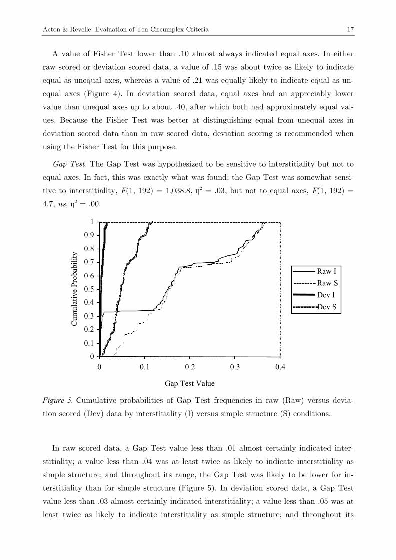
Gap Test. The Gap Test was hypothesized to be sensitive to interstitiality but not to

equal axes. In fact, this was exactly what was found; the Gap Test was somewhat sensi-

tive to interstitiality, F(1, 192) = 1,038.8, η2 = .03, but not to equal axes, F(1, 192) =

4.7, ns, η2 = .00.

0

0.1

0.2

0.3

0.4

0.5

0.6

0.7

0.8

0.9

1

0 0.1 0.2 0.3 0.4

Gap Test Value

Cum

ulat

ive

Prob

abili

ty

Raw IRaw SDev IDev S

Figure 5. Cumulative probabilities of Gap Test frequencies in raw (Raw) versus devia-

tion scored (Dev) data by interstitiality (I) versus simple structure (S) conditions.

In raw scored data, a Gap Test value less than .01 almost certainly indicated inter-

stitiality; a value less than .04 was at least twice as likely to indicate interstitiality as

simple structure; and throughout its range, the Gap Test was likely to be lower for in-

terstitiality than for simple structure (Figure 5). In deviation scored data, a Gap Test

value less than .03 almost certainly indicated interstitiality; a value less than .05 was at

least twice as likely to indicate interstitiality as simple structure; and throughout its


range, the Gap Test was likely to be lower for interstitiality than for simple structure.

Thus, the Gap Test was a useful method for distinguishing interstitiality from simple

structure.

The effect of number of variables on the Gap Test was substantial, F(1, 192) =

3,458.4, η2 = .11. This was because the Gap Test is a variance of the gaps, and although

the variance of an eight-variable circumplex will be the same as that of a 128-variable

circumplex—namely, zero—the variance of an eight-variable simple structure will be

substantially larger than that of a 128-variable simple structure, because many variables

clumping together have a small variance. The large effect of number of variables on the

Gap Test necessitated the addition of a further simulation using 8, 16, and 32 variables

(in addition to 64 and 128). The Gap Test was the only criterion to necessitate such

treatment as a result of a sizable number-of-variables effect.

Variance Test 2. VT2 was hypothesized to be sensitive to interstitiality but not to

equal axes. Indeed, VT2 was sensitive to interstitiality, F(1, 192) = 3,869.7, η2 = .17,

but not to equal axes, F(1, 192) = 24.5, η2 = .00. Deviation scoring made VT2 more

sensitive to interstitiality, F(1, 192) = 784.6, η2 = .03.

0

0.1

0.2

0.3

0.4

0.5

0.6

0.7

0.8

0.9

1

0 0.2 0.4 0.6 0.8

Variance Test 2 Value

Cum

ulat

ive

Prob

abili

ty


Figure 6. Cumulative probabilities of Variance Test 2 frequencies in raw (Raw) versus

deviation scored (Dev) data by interstitiality (I) versus simple structure (S) conditions.


In raw scored data, a VT2 value less than .25 almost certainly indicated interstitial-

ity; a value less than .30 was at least twice as likely to indicate interstitiality as simple

structure; and throughout its range, VT2 was likely to be lower for interstitiality than

for simple structure (Figure 6). In deviation scored data, a VT2 value less than .40 al-

most certainly indicated interstitiality; a value less than .58 was at least three times as

likely to indicate interstitiality as simple structure; a value less than .65 was at least

twice as likely to indicate interstitiality as simple structure; and throughout its range,

VT2 was likely to be lower for interstitiality than for simple structure (Figure 6). Thus,

VT2 was a powerful method for distinguishing interstitiality from simple structure, par-

ticularly when data were deviation scored.

VT2 was particularly sensitive to interstitiality in deviation scored data in which

there was no general factor, F(2, 192) = 298.6, η2 = .03. In raw scored data that had a

large general factor or variable general factor, VT2 was insensitive to interstitiality (al-

though the trend was in the incorrect direction). Thus, VT2 is best used with data in

which there is no general factor. In every case, deviation scoring is strongly recom-

mended.5

Rotation Test. RT is hypothesized to be sensitive to interstitiality but not to equal

axes. This was indeed what was found. The main effect of interstitiality was large, F(1,

192) = 5,261.1, η2 = .23, whereas the main effect of equal axes was negligible and was

not statistically significant. Although deviation scoring had no effect on the detection of

equal axes, it caused a pronounced improvement in the detection of interstiality, F(1,

192) = 1,265.6, η2 = .05.

In raw scored data, an RT value less than .04 almost certainly indicated interstitial-

ity; a value less than .09 was at least twice as likely to indicate interstitiality as simple

structure; and throughout its range, RT was likely to be lower for interstitiality than for

simple structure (Figure 7). In deviation scored data, an RT value less than .14 almost

certainly indicated interstitiality; a value less than .31 was at least twice as likely to

indicate interstitiality as simple structure; and throughout its range, RT was likely to

be lower for interstitiality than for simple structure (Figure 7). Thus, RT was a power-

ful method for distinguishing interstitiality from simple structure, particularly when

data were deviation scored.

5 Because VT2 was an effective circumplex criterion, whereas VT1 was not, it is recommended that in

future applications VT2 be referred to simply as the Variance Test or VT.


0

0.1

0.2

0.3

0.4

0.5

0.6

0.7

0.8

0.9

1

0 0.1 0.2 0.3 0.4

Rotation Test Value

Cum

ulat

ive

Prob

abili

ty


Figure 7. Cumulative probabilities of Rotation Test frequencies in raw (Raw) versus de-

viation scored (Dev) data by interstitiality (I) versus simple structure (S) conditions.

Minkowski Test. MT was hypothesized to be sensitive to interstitiality but not to

equal axes. This was indeed what was found. The main effect of interstitiality was large,

F(1, 192) = 6,454.8, η2 = .55, whereas the main effect of equal axes was trivial and was

not statistically significant. Although deviation scoring had no effect on the detection of

equal axes, it caused a pronounced improvement in the detection of interstitiality, F(1,

192) = 1,265.5, η2 = .11.

In raw scored data, an MT value less than .03 almost certainly indicated interstitial-

ity; a value lower than .05 was at least twice as likely to indicate interstitiality as sim-

ple structure; and throughout its range, MT was likely to be lower for interstitiality

than for simple structure (Figure 8). In deviation scored data, an RT value less than .06

almost certainly indicated interstitiality; a value less than .16 was at least twice as

likely to indicate interstitiality as simple structure; and throughout its range, MT was

likely to be lower for interstitiality than for simple structure (Figure 8). Thus, MT was

a powerful method for distinguishing interstitiality from simple structure, particularly

when data were deviation scored.


0

0.1

0.2

0.3

0.4

0.5

0.6

0.7

0.8

0.9

1

0 0.05 0.1 0.15 0.2

Minkowski Test Value

Cum

ulat

ive

Prob

abili

ty


Figure 8. Cumulative probabilities of Minkowski Test frequencies in raw (Raw) versus

deviation scored (Dev) data by interstitiality (I) versus simple structure (S) conditions.

MT was particularly sensitive to interstitiality in deviation scored data with large

sample sizes (e.g., N = 600), F(1, 192) = 65.5, η2 = .01. In raw scored data that had a

large general factor or variable general factor, MT was insensitive to interstitiality (al-

though the effect was in the incorrect direction), F(2, 192) = 364.6, η2 = .06. Thus, MT

is best used in data with large sample sizes. Where there is a general factor, the data

must be deviation scored to yield correct results. Deviation scoring is strongly recom-

mended in every case.

Discussion

The sensitivity and specificity of ten criteria for circumplex structure were tested on

simulated data sets. Five criteria contributed some valuable information, either allowing

one to reject unequal axes in favor of equal axes (Fisher Test) or allowing one to reject

simple structure in favor of circumplex structure (Gap Test, Variance Test 2, Rotation

Test, Minkowski Test).


Visible Versus Invisible Conditions

The interaction of equal versus unequal axes with interstitiality versus simple struc-

ture, which is common for tests that work, would require some theoretical explanation if

it were of appreciable size (η2 ranges from .00 to .01), because it involves only factors

that are determined by the tests, not by the investigator. Combinations of "invisible"

conditions (equal versus unequal axes, interstitiality versus simple structure, or general

factor) and "visible" conditions (e.g., deviation scoring or rotation) may require some

theoretical explanation, but they are also of practical value in manipulating real data.

For example, a visible property that can be manipulated is deviation scoring. Investi-

gators can easily use the information that deviation scoring is beneficial for manipulat-

ing and interpreting their data. This is unlike finding some interaction between equal

versus unequal axes and interstitiality versus simple structure, because these are not

manipulable but are hidden properties that investigators want to discover.

Deviation Scoring: Boon or Blight?

With respect to the visible properties, the goal is to make some sort of practical rec-

ommendation for manipulating and interpreting data—if possible, one that applies gen-

erally to all of the criteria that work. A finding that generalizes across most criteria is

that deviation scoring makes criteria better at doing what they were created to do—

although it cannot enable them to do what they were not created to do. Deviation scor-

ing works because it removes a general factor if there is one and has little effect if there

is not. If the data are perfectly circumplexical, then the sum of all items is zero and de-

viation scoring will have no effect. If the data have a general factor, then the sum of all

items is greater than zero and deviation scoring will reduce the general factor.

Deviation scoring can actually prevent the Variance Test 2 from rendering incorrect

results. When raw scored data have a large general factor or a variable general factor,

VT2 will mislabel a simple structure as an interstitial structure. Because deviation scor-

ing reduces a general factor, it allows VT2 to render the results it would otherwise ren-

der in raw scored data with no general factor, namely a correct identification of intersti-

tiality versus simple structure.

The Gap Test is hypothesized to be able to detect interstitiality; although it can do

this without deviation scoring, it can do it even better with deviation scoring. It is not

hypothesized to be able to detect equal axes, nor can it; deviation scoring in some cases

actually causes it to register the opposite of the correct result (although these are weak


trends). Thus, deviation scoring is a mixed blessing: Used with the correct interpreta-

tion, it can enhance the power of a test; used with an incorrect interpretation, it can

render fallacious results.

There are many three-way interactions involving deviation scoring. In some, devia-

tion scoring makes a good test better. In others (such as interstitiality x deviation scor-

ing x general factor in VT2, discussed above), deviation scoring makes a bad test good.

In the interest of keeping things simple, we have looked at the main effects of equal

axes and interstitiality and the two-way interactions of equal axes x deviation scoring

and interstitiality x deviation scoring. Those that are of non-negligible size and are sta-

tistically significant (using a stringent alpha level of .0001) warrant further considera-

tion; the others (SQLI, Gap*, GDIFF, CDIFF, and VT1) can be ignored.

The data presented herein provide ample documentation for a broad conclusion re-

garding deviation scoring: Used properly, deviation scoring is a circumplex researcher's

best friend. Deviation scoring is especially beneficial if one has no way of knowing a pri-

ori whether the data contain a general factor, which may be typical of real-life circum-

stances. This is an important qualification, because all of the analyses presented herein

are predicated on the assumption that one does not know whether or not the data have

a general factor. Thus, the criteria that are said to work are useful primarily for ex-

ploratory purposes6.

A Hierarchy of Models

A circumplex falls somewhere in the middle of a hierarchy of models. The hierarchy,

in order of descending parsimony, is as follows:

(a) one factor;

(b) multiple factors but simple structure;

(c) multiple factors with some interstitial variables;

6 When there is a general factor that is not removed through deviation scoring or some other procedure,

rotation will have the effect of eliminating a circumplex where one exists. Nevertheless, we have called a

condition characterized by a circumplex plus a general factor a circumplex condition, even when rotated,

because a researcher normally cannot know a priori whether there is a general factor in the data. The

general factor condition is considered an invisible condition because, although some general factors can be

identified as the first extracted factor, on which all variables have positive loadings, other, more subtle

general factors simply elevate bipolar factor loadings and therefore are not easily detectable.


(d) multiple factors and variables show equal spacing around pairs of factors;

(e) multiple factors and all items are best described in terms of more than two factors.

Model d (which includes the circumplex) falls somewhere between model c and model

e in degree of parsimony. If an instrument can be characterized by models a, b, or e,

then it is not a circumplex. Having multiple factors with some interstitial variables

(model c) is a necessary but not sufficient condition for an instrument to be a circum-

plex. In a circumplex (model d) the variables must also be equally spaced.

Although a circumplex is less parsimonious than a two-dimensional simple structure

or a one-dimensional test, it may also be a more accurate reflection of a complex field.

It would be easy to devise a simple structure made up of variables measuring two unre-

lated domains, such as hardness and brightness. It is much more difficult to devise a

circumplex structure, because one must sample from a complex domain made up of in-

terrelated variables. The latter, although less parsimonious, would be a more significant

finding than the former.

Examples of complex domains are affective states and interpersonal traits. It is possi-

ble to feel emotions that are subtle combinations of valence and arousal; for example,

excitement is a positive emotion that also reflects high arousal. It is also possible to be-

have toward others in ways that are subtle combinations of dominance and friendliness;

for example, gregariousness is a friendly trait that also reflects high dominance. In each

case, the particular item is drawn from a complex domain comprised of interrelated

subdomains. Where such interrelationships exist, it is desirable that they be discovered.

The present study has provided new and effective means of doing so.

Limitations

The simulations presented herein are based on idealized conditions. An attempt was

made, however, to represent not only a diversity of idealized conditions, but also condi-

tions that actually appear in practice. Thus, although the application of these results

may be limited to cases similar to those included in the simulation, such cases do occur.

The differences between the interstitiality versus simple structure conditions and the

equal versus unequal radius conditions were designed to be large enough that one could

distinguish them by inspection of the plot of variables in the factor space. Several crite-

ria failed this evaluation, and these failures may be as revealing as the successes. Never-

theless, although further research on the criteria that worked seems warranted, these

criteria can be recommended as having passed their first important test.


References

Acton, G. S., & Revelle, W. (2002). Interpersonal personality measures show circumplex

structure based on new psychometric criteria. Journal of Personality Assessment,

79, 446-471.

Alden, L. E., Wiggins, J. S., & Pincus, A. L. (1990). Construction of circumplex scales

for the Inventory of Interpersonal Problems. Journal of Personality Assessment, 55,

521-536.

Browne, M. W. (1992). Circumplex models for correlation matrices. Psychometrika, 57,

469-497.

Conte, H. R., & Plutchik, R. (1981). A circumplex model for interpersonal personality

traits. Journal of Personality and Social Psychology, 40, 701-711.

Dryer, D. C., & Horowitz, L. M. (1997). When do opposites attract? Interpersonal com-

plementarity versus similarity. Journal of Personality and Social Psychology, 72,

592-603.

Fabrigar, L. R., Visser, P. S., & Browne, M. W. (1997). Conceptual and methodological

issues in testing the circumplex structure of data in personality and social psychol-

ogy. Personality and Social Psychology Review, 1, 184-203.

Fisher, G. A. (1997). Theoretical and methodological elaborations of the circumplex

model of personality traits and emotions. In R. Plutchik & H. R. Conte (Eds.), Cir-

cumplex models of personality and emotions (pp. 245-269). Washington, DC: Ameri-

can Psychological Association.

Gurtman, M. B. (1993). Constructing personality tests to meet a structural criterion:

Application of the interpersonal circumplex. Journal of Personality, 61, 237-263.

Gurtman, M. B. (1994). The circumplex as a tool for studying normal and abnormal

personality: A methodological primer. In S. Strack & M. Lorr (Eds.), Differentiating

normal and abnormal personality (pp. 243-263). New York: Springer.

Gurtman, M. B., & Pincus, A. L. (2000). Interpersonal Adjective Scales: Confirmation

of circumplex structure from multiple perspectives. Personality and Social Psychol-

ogy Bulletin, 26, 374-384.

Guttman, L. (1954). A new approach to factor analysis: The radex. In P. F. Lazarsfeld

(Ed.) Mathematical thinking in the social sciences (pp. 258-348). Glencoe, IL: Free

Press.


Hofstee, W. K. B., de Raad, B., & Goldberg, L. R. (1992). Integration of the Big Five

and circumplex approaches to trait structure. Journal of Personality and Social Psy-

chology, 63, 146-163.

Hubert, L. J., & Arabie, P. (1987). Evaluating order hypotheses within proximity ma-

trices. Psychological Bulletin, 102, 172-178.

Johnson, J. A., & Ostendorf, F. (1993). Clarification of the five-factor model with the

abridged Big Five-dimensional circumplex. Journal of Personality and Social Psy-

chology, 65, 563-576.

Larsen, R. J., & Diener, E. (1992). Promises and problems with the circumplex model of

emotion. In M. S. Clark (Ed.), Review of personality and social psychology: Emotion

(Vol., 13, pp. 25-59). Newbury Park, CA: Sage.

Locke, K. D. (2000). Circumplex Scales of Interpersonal Values: Reliability, validity,

and applicability to interpersonal problems and personality disorders. Journal of

Personality Assessment, 75, 249-267.

Locke, K. D. (2003). Status and solidarity in social comparison: Agentic and communal

values and vertical and horizontal directions. Journal of Personality and Social Psy-

chology, 84, 619-631.

Markey, P. M., Funder, D. C., & Ozer, D. J. (2003). Complementarity of interpersonal

behaviors in dyadic interactions. Personality and Social Psychology Bulletin, 29,

1082-1090.

Plutchik, R., & Conte, H. R. (Eds.; 1997). Circumplex models of personality and emo-

tions. Washington, DC: American Psychological Association. Revelle, W., & Rocklin, T. (1979). Very simple structure: An alternative procedure for

estimating the optimal number of interpretable factors. Multivariate Behavioral Re-

search, 14, 403-414.

Saucier, G. (1992). Benchmarks: Integrating affective and interpersonal circles with the

Big-Five personality factors. Journal of Personality and Social Psychology, 62, 1025-

1035.

Saucier, G., Ostendorf, F., & Peabody, D. (2001). The non-evaluative circumplex of

personality adjectives. Journal of Personality, 69, 537-582.

Schaefer, E. S. (1997). Integration of configurational and factorial models for family re-

lationships and child behavior. In R. Plutchik & H. R. Conte (Eds.), Circumplex

models of personality and emotions (pp. 133-153). Washington, DC: American

Psychological Association.


Shepard, R. N. (1962). Analysis of proximities: Multidimensional scaling with an un-

known distance function II. Psychometrika, 27, 219-246.

Soldz, S., Budman, S., Demby, A., & Merry, J. (1993). Representation of personality

disorders in circumplex and five-factor space: Explorations with a clinical sample.

Psychological Assessment, 5, 41-52.

Thurstone, L. L. (1947). Multiple factor analysis. Chicago: University of Chicago Press.

Tracey, T. J. G. (1997). RANDALL: A Microsoft FORTRAN program for a randomiza-

tion test of hypothesized order relations. Educational and Psychological Measure-

ment, 57, 164-168.

Tracey, T. J. G. (2000). Analysis of circumplex models. In H. E. A. Tinsley & S. D.

Brown (Eds.), Handbook of applied multivariate statistics and mathematical modeling

(pp. 641-664). San Diego, CA: Academic.

Tracey, T. J. G., & Rounds, J. B. (1993). Evaluating Holland's and Gati's vocational-

interest models: A structural meta-analysis. Psychological Bulletin, 113, 229-246.

Trobst, K. K. (2000). An interpersonal conceptualization and quantification of social

support transactions. Personality and Social Psychology Bulletin, 26, 971-986.

Upton, G. J. G., & Fingleton, B. (1989). Spatial data analysis by example: Vol. 2. Cate-

gorical and directional data. New York: Wiley.

Wagner, C. C., Kiesler, D. J., & Schmidt, J. A. (1995). Assessing the interpersonal

transaction cycle: Convergence of action and reaction interpersonal circumplex

measures. Journal of Personality and Social Psychology, 69, 938-949.

Wiggins, J. S., Steiger, J. H., & Gaelick, L. (1981). Evaluating circumplexity in person-

ality data. Multivariate Behavioral Research, 16, 263-289.

Yik, M. S. M., Russell, J. A., & Feldman Barrett, L. (1999). Structure of self-reported

current affect: Integration and beyond. Journal of Personality and Social Psychol-

ogy, 77, 600-619.

Evaluation of Ten Psychometric Criteria for Circumplex ...€¦ · Evaluation of Ten Psychometric...

Documents

Transcript of Evaluation of Ten Psychometric Criteria for Circumplex ...€¦ · Evaluation of Ten Psychometric...