I. Report No. 2. Government Accession No.

FHW AffX-00/1715-S

4. Title and Subtitle

EVALUATION OF SOME EXISTING TECHNOLOGIES FOR VEHICLE DETECTION

7. Author(s)

Dan Middleton, Debbie Jasek, and Ricky Parker

9. Perfomring Organization Name and Address

Texas Transportation Institute The Texas A&M University System College Station, Texas 77843-3135

12. Sponsoring Agency Name and Address

Texas Department of Transportation Research and Technology Transfer Office P. 0. Box 5080 Austin, Texas 78763-5080

15. Supplementary Notes

Technical Reoort Documentation Pag•

3. Recipient's Catalog No.

5. Report Date

September 1998 Resubmitted: September 1999

6. Performing Organization Code

8. Performing Organization Report No.

Report 1715-S ~~~~~~~~--;

. (TRAIS)

11. Contract or Grant No.

Project No. 0-1715

13. Type of Report and Period Covered

Project Summary: September 1996-August 1999

14. Sponsoring Agency Code

Research performed in cooperation with the Texas Department of Transportation and the U.S. Department of Transportation, Federal Highway Administration. Research Project Title: Evaluation of the Existing Technologies for Vehicle Detection

16. Abstract

Most vehicle detection today relies on inductive loop detectors (ILDs). However, problems with installation and maintenance of these detectors have necessitated evaluation of alternative detection systems. Replacing ILDs with better detectors requires a thorough evaluation of the alternatives. This evaluation included examination of the functional quality, reliability, and cost of these technologies as well as development of recommendations for application. Primary detection technologies included in this study are video image detection systems (VIDS), passive infrared, active infrared, passive magnetic, radar, Doppler microwave, passive acoustic, and ILDs. Results of new detector testing clearly indicate promising alternatives to ILDs, but the limitations of these new detectors must also be accepted. Researchers found that some technologies performed quite well while, in some cases, offering features that are more flexible than ILDs. These technologies include VIDS, passive infrared, active infrared, radar, Doppler microwave, and pulse ultrasonic.

17. KeyWords 18. Distribution Statement

Non-intrusive Detectors, Sensor Technologies, Vehicle Detection, Inductive Loop Detectors

No restrictions. This document is available to the public through NTIS:

19. Security Classif. (of this report)

Unclassified Form DOT F 1700.7 (8-72)

National Technical Information Service 5285 Port Royal Road Springfield, Virginia 22161

20. Security Classif.(ofthis page)

Unclassified Reproduction of completed page authorized

21. No. of Pages

184 22. Price

. . EVALUATION OF SOME EXISTING TECHNOLOGIES

FOR VEIDCLE DETECTION

by

Dan Middleton Program Manager

Texas Transportation Institute

Debbie Jasek Assistant Research Specialist Texas Transportation Institute

and

Ricky Parker Engineering Research Associate Texas Transportation Institute

Report 1715-S Project Number 0-1715

Research Project Title: Evaluation of the Existing Technologies for Vehicle Detection and Establishment of Communication Data Requirements

Sponsored by the Texas Department of Transportation

In Cooperation with the U.S. Department of Transportation Federal Highway Administration

September 1998 Resubmitted: September 1999

TEXAS TRANSPORTATION INSTITUTE The Texas A&M University System College Station, Texas 77843-3135

DISCLAIMER

The contents of this report reflect the views of the authors, who are responsible for the opinions, findings, and conclusions presented herein. This project was conducted in cooperation with the U.S. Department of Transportation, Federal Highway Administration. The contents do not necessarily reflect the official views or policies of the Federal Highway Administration or the Texas Department of Transportation. This report does not constitute a standard, specification, or regulation.

NOTICE

The Unites States Government and the state of Texas do not endorse products or manufacturers. Trade or manufacturers' names appear herein solely because they are considered essential to the object of this report.

v

ACKNOWLEDGMENTS

The authors wish to gratefully acknowledge the contributions of several persons who made the successful completion of this research possible. This especially includes the project directors, Mr. Abed Abukar and Ms. Lilly Banda. Special thanks are also extended to employees of all the Texas Department of Transportation districts that participated in the survey, as well as personnel of out-of-state agencies who participated.

vi

TABLE OF CONTENTS

Page

LIST OF FIGURES .. ..... .. . . .. . . ... . .. . .. . . .. . . . . . . . . .. . . . ......... ........... ... ... . ......... .. ... . . .. .. . ... .. ....... .. . .. . . . . xii LIST OF TABLES ............................................................................................................... xiii IMPLEMENTATION RECOMMENDATIONS ................................................................. xv

1.0 IN1RODUCTION ............ ...... .............. ...... ...................... ...................... ...... ................... 1 1.1 BACKGROUND.................................................................................................. 1 1.2 RESEARCH FOCUS ...................................... .......... ................. ................. ... ...... 1 1.3 RESEARCH OBJECTNES ...................... .......... ......... ..................... .................. 2 1.4 METHODOLOGY............................................................................................... 2

1.4.1 Literature Search and Review.................................................................. 2 1.4.2 Survey of State Practices ....... ...... ............................................................ 2 1.4.3 Evaluation of Existing Technologies for Vehicle Detection ................... 3 1.4.4 Comparison of Functional Quality and Reliability of

Loops vs. Other Detection Technologies ................................................ 3 1.4.5 Cost Analysis of Various Vehicle Detection Technologies ..................... 3 1.4.6 Evaluate and Develop Data Exchange Requirements for

the Transmission of Vehicle Detector Information................................. 3 1.4.7 Recommendations of Technologies to Appropriate

Applications . . .. . .. ......... ... . . . . . ... . ..... ... .. .. . ... . .. . .. . ...... ... ..... .. . .. . .. . .. ....... ..... .. .. 3 1.4.8 Develop Specifications for the Detectors ......................................... ....... 4

2.0 LITERATURE REVIEW................................................................................................. 5 2.1 IN1RODUCTION ................................................................................................ 5 2.2 DETECTOR PERFORMANCE FINDINGS....................................................... 5

2.2.1 Inductive Loop Detectors......................................................................... 5 2.2.2 Video Image Detection Systems.............................................................. 5

2.2.2.1 California Polytechnic State University Research .............................. 5 2.2.2.2 Hughes Aircraft Research ............................... ................................... 6 2.2.2.3 Jet Propulsion Laboratory Research ....... ... ... .. ... . . . . ... .. ........ .. ... .... .. . ... 6 2.2.2.4 Minnesota Guides tar Research ............................... ........................... 7

2.2.3 Active Infrared Detectors......................................................................... 8 2.2.4 Passive Infrared Detectors....................................................................... 9 2.2.5 Radar Detectors ....... .. . .. . . . .. .. . ........... .. .. . . .. . ... ... ... ........ .. .. . . . . ... .. ......... .. .. . .. . 9 2.2.6 Microwave Detectors.............................................................................. 10 2.2.7 Passive Acoustic Detectors ..................................................................... 10 2.2.8 Pulse Ultrasonic Detectors ...................................................................... 11 2.2.9 Other Detectors ....................................................................................... 11

vii

TABLE OF CONTENTS (Continued)

Page

3.0 ACCURACY AND RELIABILITY OF DETECTORS ............................................... 13 3 .1 INTRODUCTION............................................................................................ 13 3.2 ACCURACY AND RELIABILITY OF INDUCTNE LOOPS ...................... 13

3.2.1 Experience in Texas............................................................................. 13 3.2.1.1 TxDOT Districts............................................................................. 13 3 .2.1.2 TransGuide Data ............................................................................ 16 3.2.1.3 TTI Freeway Test Bed in College Station...................................... 17 3 .2.1.4 US 290 in Houston . . .. . . .. . . . .. . ........... .. . . . .. . . .. . .. .. .. ......... .. .. .. .. . .. .. .. .. ... . 19 3.2.l.5 IH-20 in Ft. Worth.......................................................................... 19

3 .2.2 Experience in Other States................................................................... 19 3.2.3 Loop Experience in Europe................................................................. 21

3.3 ACCURACY AND RELIABILITY OF NON-INTRUSNE DETECTORS ............................................................................................... 22 3.3.1 Accuwave 150LX Presence Detector.................................................. 24

3.3.1.1 Accuwave Introduction.................................................................. 24 3.3.1.2 Accuwave Setup............................................................................. 25 3.3 .1.3 Accuwave Results ..................... ..................... ................................ 25 3.3.1.4 Accuwave Conclusions.................................................................. 26

3.3.2 Nestor Traffic Vision Video Detector.................................................. 26 3.3.2.1 Nestor Introduction......................................................................... 26 3.3.2.2 Nestor Setup................................................................................... 26 3.3.2.3 Nestor Results ................................................................................ 27 3.3.2.4 Nestor Conclusions ....................................................................... .

3.3.3 PIR-1 Passive Infrared Detector ......................................................... . 3.3.3.1 PIR-1 Introduction ......................................................................... .

28 28 28

3.3.3.2 PIR-1 Setup.................................................................................... 28 3.3.3.3 PIR-1 Results.................................................................................. 28 3 .3 .3 .4 PIR-1 Conclusions.......................................................................... 29

3.3.4 RTMS Detector.................................................................................... 30 3.3.4.1 RTMS Introduction........................................................................ 30 3.3.4.2 RTMS Setup................................................................................... 30 3.3.4.3 RTMS Results................................................................................ 31 3.3.4.4 RTMS Conclusions ....................................................................... .

3.3.5 SmartSonic Acoustic Detector ............................................................ . 3.3.5.1 SmartSonic Introduction ............................................................... . 3.3.5.2 SmartSonic Setup .......................................................................... . 3.3.5.3 SmartSonic Results ....................................................................... . 3.3.5.4 SmartSonic Conclusions ............................................................... .

viii

31 31 31 31 31 31

TABLE OF CONTENTS (Continued)

Page

3.3.6 Tests on High-Volume Freeways ........................................................ 32 3.3.6.1 Houston Field Tests ....................................................................... 32 3.3.6.2 Ft. Worth Field Tests ..................................................................... 34

3.3.7 Overall Field Test Conclusions .......................................................... 35 3.3.8 Experience of RCOC with Autoscope................................................. 35

3.3.8.1 Camera Mounting Considerations.................................................. 35 3.3.8.2 System Accuracy............................................................................ 36

3.3.9 TxDOT Experience.............................................................................. 36 3.4 SUMMARY OF DETECTOR ACCURACY

AND RELIABIIJTY ........................................ ..................................... ....... 37

4.0 COST ANALYSIS OF VEHICLE DETECTION TECHNOLOGIES ........................ 39 4.1 INTRODUCTION............................................................................................ 39 4.2 TXDOT DISTRICT INDUCTIVE LOOP COSTS.......................................... 39

4.2.l Houston Inductive Loop Costs............................................................ 40 4.2.1.1 Houston Signalized Intersection Inductive Loop Costs................. 40 4.2.1.2 Houston Freeway Inductive Loop Costs . ......................... ..... ......... 41

4.2.2 Waco Inductive Loop Costs................................................................. 43 4.2.3 Paris Inductive Loop Costs.................................................................. 43

4.3 NON-INTRUSIVE DETECTION COSTS...................................................... 44 4.3.1 Video Image Detection Systems.......................................................... 44

4.3.1.1 Out-of-State Cost Information........................................................ 44 4.3.1.2 TxDOT District Cost Information.................................................. 45

4.3.2 Non-VIDS Detector Systems............................................................... 46 4.3.2.1 Accuwave Detector......................................................................... 46 4.3.2.2 Passive Infrared Detector............................................................... 46 4.3.2.3 RTMS Detector.............................................................................. 46 4.3.2.4 SmartSonic Acoustic Detector....................................................... 47

4.4 COMPARISON OF ILD COSTS AND OTHER DETECTION COSTS .................................................................................. 47 4.4.1 Literature Sources................................................................................ 47 4.4.2 Study 0-1715 Findings......................................................................... 47

4.4.2.1 Houston ... ....................................................................................... 48 4.4.2.2 Paris................................................................................................ 48 4.4.2.3 Waco............................................................................................... 49

4.5 SUMMARY OF COST COMPARISONS ...................................................... 49

IX

TABLE OF CONTENTS (Continued)

Page

5.0 NATIONAL TRANSPORTATION COMMUNICATIONS FOR ITS PROTOCOL (NTCIP) AND TRANSPORTATION SENSOR SYSTEM DEVELOPMENT . ................................................................ 51 5.1 INTRODUCTION............................................................................................ 51 5.2 DEVELOPMENT IDSTORY .......................................................................... 51 5.3 TRAFFIC SENSOR SYSTEM........................................................................ 51 5.4 STANDARD TERMS AND DEFINITIONS................................................... 52

5.4.1 Description of Zone and Virtual Zone................................................. 53 5.4.2 Description of a Sensor and TSS Deployments................................... 53

5.5 CONFORMITY GROUPS............................................................................... 54 5.6 NTCIP WORKING GROUP DEVELOPMENTS

TO DA TE AND FUTURE PLANS.............................................................. 55

6.0 APPLICATIONS GUIDE TO Th1PLEMENTATION.................................................. 57 6.1 INTRODUCTION............................................................................................ 57 6.2 FINDINGS ................................................................ ..... ... .... ....................... .... 57 6.3 IMPLEMENTATION ........................................................ ....... .................... ... 58

6.3.1 Based on Literature Findings............................................................... 58 6.3.2 Based on Surveys and TTI Field Tests................................................ 59

6.3.2.1 Accuwave 150LX Microwave Detector......................................... 59 6.3.2.2 Autoscope VIDS Detector.............................................................. 59 6.3.2.3 Nestor Traffic Vision VIDS Detector.............................................. 60 6.3 .2.4 PIR-1 Passive Infrared Detector..................................................... 60 6.3.2.5 RTMS Microwave Radar Detector................................................. 61 6.3.2.6 SmartSonic Passive Acoustic Detector.......................................... 61 6.3.2.7 Overall Results............................................................................... 62

7 .0 REFERENCES............................................................................................................. 67

8.0 APPENDIX A INSTALLATION AND MAINTENANCE OF INDUCTIVE LOOP DETECTORS ............................................................................................. 71

9 .0 APPENDIX B GRAPIDCAL RESULTS OF COLLEGE STATION FIELD TESTS................... 87

10.0 APPENDIX C GRAPIDCAL RESULTS OF HOUSTON FIELD TESTS.................................. 121

x

TABLE OF CONTENTS (Continued)

Page

11.0 APPENDIX D SPECIFICATION FOR VIDS DETECTORS..................................................... 139

12.0 APPENDIX E SPECIFICATION FOR MICROWAVE DETECTORS...................................... 163

xi

LIST OF FIGURES

Figure Page

3-1 TTI Test Site in College Station.............................................................................. 18 3-2 SH 6 Test Site Showing Pole and Mast Arm.......................................................... 23 3-3 PIR-llnterfaceCircuit ............................................................................................ 29 5-1 Sensor and Zone Description.................................................................................. 53 5-2 NTCIP TSS Functional Diagram............................................................................ 54

xii

LIST OF TABLES

Table Page

3-1 TxDOT District 11.,D Summary............................................................................... 14 3-2 Accuwave Setup Events.......................................................................................... 25 3-3 Nestor Setup Events................................................................................................ 27 3-4 PIR-1 Setup Events ....... ............................ ...... .............................. ...................... .... 29 3-5 RTMS Setup Events................................................................................................ 30 3-6 11.,D Accuracy and Failure Rate............................................................................... 37 3-7 Non-Intrusive Detector Count Accuracy Based on TTI Field Tests ....................... 38 4-1 Replacement Cost for Failed Loops at Intersections. in the

Houston District .. . . . .. . . . . .. . . . ....... ...... .. . . . . . .. . ... ......... .. . .. .. .. .. .. . ......... .. .. . .. . . . ... . .. ..... ... 40 4-2 Cost of Installation and Replacement of Houston Freeway Loops ......................... 42 4-3 Summary of Monthly Maintenance Costs of Four RCOC Systems........................ 45 4-4 Accuwave and PIR-1 Annual Costs ....................................................................... 4 7 4-5 TxDOT 11.,D Costs Compared to VIDS Costs...................................................... .. 50 4-6 Detector Annualized Total Cost Comparisons........................................................ 50 4-7 Freeway Detector Annualized Per-Lane Cost Comparison..................................... 50 6-1 Quantitative Evaluation of Detectors at Signalized Intersections ........................... 63 6-2 Quantitative Evaluation of Detectors on Freeways................................................. 64 6-3 Application Guide for Detector Selection at Signalized Intersections................... 65 6-4 Application Guide for Detector Selection on Freeways......................................... 66

xiii

IMPLEMENTATION RECOMMENDATIONS

The objective of this research study was to evaluate new detector technologies through a literature search, a survey of TxDOT districts and out-of-state agencies, and full-scale field tests. The implementation recommendations for this project are based on these findings.

1. In Minnesota Guidestar tests, the RTMS (true presence microwave) was easily mounted but required a moderate amount of calibration to achieve optimal performance. At the freeway site, it undercounted vehicles by 2 percent or less in the overhead position and 5 percent in the sidefire position. It was not tested at the intersection site.

2. Minnesota tests included two pulse ultrasonic detectors, the Microwave Sensors TC-30 and the Novax Lane King. Both were relatively easy to mount, but the Lane King required more extensive calibration. Weather conditions did not impact the performance of the devices, and either device can mount overhead or sidefire. Both detectors overcounted vehicles stopped at the intersection, counting individual vehicles multiple times. The Lane King was extremely accurate in counting vehicles at the freeway site.

3. Video image detection system (VIDS) testing in Minnesota included the Peek Transyt VideoTrak:-900, the Autoscope 2004, and the Eliop Trafico EV A 2000 (freeway application only). Lighting variations and shadows were the most significant weather­related conditions that affected video devices. The count accuracies of the Peek Trak:-900 were within 5 percent of baseline on the freeway, but periodic failures occurred during intersection tests. The Autoscope performed within 5 percent accuracy at both freeway and intersection test sites, although light transitions resulted in undercounting.

4. Hughes Aircraft research results favored Doppler microwave detectors, but this technology does not detect stopped vehicles. The Doppler microwave, true presence microwave (RTMS), visible VIDS, SPVD magnetometer, and inductive loop technologies performed well for low-volume counts (JO).

5. For high-volume counts, the Doppler microwave, true presence microwave, visible VIDS, and inductive loops performed well. The Doppler microwave was the best performing technology for speed accuracy in both low- and high-volumes. The Doppler microwave, true presence microwave (RTMS), SPVD magnetometer, and inductive loop technologies performed best in inclement weather ( 10).

6. Duckworth et al. (5) tests indicated that VIDS had limitations in poor lighting and certain weather conditions, and was the most expensive sensor tested. Pulsed ultrasound was best for detection and classification when cost, the communications bandwidth requirements, and processing power were considered. Radar was the best speed sensor for vehicles it detected (5).

xv

7. , Field tests at the Texas Transportation Institute freeway test bed included inductance loop detectors (ILD) for baseline data, Accuwave (microwave), Nestor Traffic Vision (VIDS), RTMS (true presence microwave), SmartSonic (acoustic), and PIR-1 (passive infrared). Count accuracy of the ILDs was within 2 percent of manual counts using repetitive review of video tapes. With the exception of the RTMS, test detectors exhibited count errors as high as 20 to 50 percent. The worst count error observed with the RTMS was 15 percent for only one hour, with the remainder falling within 10 percent.

8. Field tests on US 290 in Houston provided additional performance data to supplement College Station tests. Testing included the Nestor Traffic Vision, the Autoscope 2004, and the RTMS. Detector performance was more erratic in higher volumes where traffic was very congested during parts of the day.

9. Lane 1 Autoscope counts in Houston from 6:00 a.m. to midnight were generally within 10 percent of baseline counts. Many of the 15-minute counts were within 5 percent. Counts after darkness were the exception, with the Autoscope overcounting by as much as 30 to 40 percent. Lane 2 counts were more erratic than lane 1 counts. Daylight errors were both positive and negative in the range of plus 20 percent to minus 50 percent. Nighttime errors were even worse. Lane 3 daylight errors were in the plus 20 to minus 30 percent range, and nighttime errors were again worse. A better camera and camera position would probably improve these results.

10. In Houston tests, the Nestor both overcounted and undercounted vehicles in lane 1 by 30 percent during daylight hours. There were many time periods during the daytime when its count error was in the zero to 10 percent range. A better camera and camera position would probably improve these results.

11. RTMS performance in Houston was apparently not affected by changing light conditions. Therefore, its count performance during early morning and late afternoon light transition periods was similar to its mid-day performance. It generally undercounted lane 1 traffic by 5 to 10 percent. In lane 2, the RTMS mostly overcounted in the range of up to 10 percent. On two days, it also undercounted traffic in lane 2 but usually by no more than 5 percent. Lane 3 counts showed no bias toward overcounting or undercounting for most time periods, with errors in the range of 10 percent. RTMS performance was unaffected by the distance of the pole from the roadway.

12. The difficulty in finding suitable test sites in Houston and Ft. Worth emphasized the need to identify and instrument urban test beds for future tests. Important factors are: a properly positioned pole, working trap loops in each lane, good alignment, flat profile, minimal weaving and lane changing, and an equipment cabinet.

xvi

13. ILD accuracy and durability is directly attributable to rigid specifications and an aggressiye inspection and test program. There is an immediate need for TxDOT to improve on these items. Examples in Europe are The Netherlands with a failure rate of one per 1,500 loops. Switzerland experienced a loss of five per 200.

14. Comparisons of costs of detection on freeways indicate that loops and VIDS are approximately equal for a six-lane freeway, but loops are more expensive if motorist delay is included. The second most expensive technology would then be VIDS, while the most cost-effective device evaluated in research project 0-1715 was the RTMS if deployed in the sidefire mode. It increases in viability with greater numbers of lanes, because in the sidefire mode, it can monitor up to eight lanes. Its mounting requirements are also less stringent than VIDS or most other devices.

15. The type and quality of the video sensor (camera) for a VIDS dictates the accuracy of the system. A monochrome camera is 10 times more sensitive to light than a color camera, so for low light levels or at night, monochrome cameras perform better and have higher resolution than color cameras. Without an automatic iris in the camera lens, changing ambient light conditions will cause the camera's output to the VIDS to be useless. Also, an infrared filter on the camera lens reduces glare from the sun and headlights at night, thereby increasing detection accuracy.

xvii

OPERATIONAL AND SAFETY ANALYSIS . .

The Texas Transportation Institute (TTI) conducted operational and safety assessments of two basic scenarios proposed for S.R. 60 in Los Angeles, California. "Scenario l" accommodates trucks in the mixed flow lanes, while "Scenario 2" provides an exclusive truck facility that runs the full length of the study corridor. Realizing that Scenario 2 involves two flows of traffic, TTI designated the mixed lanes as 2(A) and the truck facility as 2(B). Analyses and results that follow will refer to each accordingly.

The study segment of S.R. 60, approximately 35 miles in length, currently serves significant east-west truck traffic throughout this length from I-710 on the west to Etiwanda Avenue on the east (just east of I-15). Traffic assignment from SCAG's regional model for Year 2020 provided the basis of all evaluations. HDR Engineering, Inc. provided preliminary plan drawings of interchanges.

OPERATIONAL ANALYSIS METHODOLOGY

This operational analysis utilized the 1997 Update to the Highway Capacity Manual (HCM) (I) or Transportation Research Board Special Report 209, and its companion software, the Highway Capacity Software (HCS), Release 3. The HCM is the recognized authority in formulation of analyses for various categories of roadways and intersections. For many years, the HCM has provided the technical information and procedures necessary to determine the quality of operation, referred to as "Level of Service," for freeways and other roadways.

The HCS is supported by the Federal Highway Administration (FHW A) and is available through the McTrans Center for Microcomputers in Transportation at the University of Florida Transportation Research Center. The HCS consists of many modules; the module names used for this project correspond to the system elements being evaluated (e.g. Basic Freeway Segment).

The evaluation of each scenario began by segmenting the freeway into sections that have similar characteristics and that also correspond to segments selected for other aspects of this project. Processing of freeway components began with "Basic Freeway Sections," followed by "Ramps," and concluded with consideration of "Weaving Analysis." The appropriate criteria for selecting mainline segments for the operational analysis include traffic volume, truck volume, grades, number of lanes, and interchange density. Once these segments were established, analysts selected the critical (largest) 2020 assignments on those segments to be used in the HCS.

Derivation of Truck Lane Capacity

Various assumptions and variables are necessary to run the HCS successfully, and these variables must accurately reflect the features of the roadway that affect operations. One of the critical variables in this discussion related specifically to trucks and other large vehicles is Passenger Car Equivalents (PCE). The HCM defines PCE as "The number of passenger cars that are displaced by a single heavy vehicle of a particular type under prevailing roadway, traffic, and control conditions."

1

The mathematical expression for the factor used in the HCM for calculation of the "heavy vehicle factor" is:

' fHV l/[l + Pi{ET- l)]

Where: fHV = heavy vehicle factor, PT= percent trucks in the traffic stream, and ET is the passenger car equivalency of trucks in the traffic stream. The fHV factor converts from PCBs to vehicles and vice-versa.

Reasons PCBs are critical in this analysis include the fact that trucks are larger and have different operating characteristics compared to cars, and Scenario 2 includes a facility that is designed for 100 percent trucks. Neither the current HCM nor materials proposed by Penn State University for the HCM 2000 (2) contain evaluation methodology for truck flows that exceed 25 percent of the traffic stream. On the truck facility, trucks are 100 percent of the traffic stream.

CORSIM to Determine PCE. Because the HCM procedures included PCB values only up to 25 percent, TTI used the simulation software, CORSIM, to develop PCBs for 100 percent trucks on controlled access facilities. CORSIM is an FHW A corridor microscopic simulation model that is based on the older FRESIM and NETSIM models. It simulates traffic networks by moving individual vehicles through a combined surface street and freeway network. It is currently available through the McTrans Center under the name Traffic Software Integrated System/Corridor-Microscopic Simulation (TSIS/CORSIM). The analysis involved coding 15 segments using 2020 assignments for mainline links only. Coding the entire network of all ramps and the mainline for the entire corridor would have been much too time consuming and unnecessary. The intent for its use was only to check PCB values for use in the HCS software.

Comparing a few PCB values from the Penn State research and the 1997 HCM values for various truck percentages and "Specific Upgrades" yielded results that were useful. In HCM tabulated values, higher percentages of trucks for a selected grade (grade range 0 percent to 3 percent in the S.R. 60 corridor) result in either a flat or downward trend in PCB values. This means that higher percentages of trucks tend to interfere less on a per-vehicle basis with each other and with other vehicles in the traffic stream than a few trucks. The HCM values for flat grades and for 3 percent grades (over 1.5 miles in length) at 25 percent trucks are 1.5 and 3.0, respectively. It should also be noted that the HCM promotes the values of 1.5 and 3.0 in "Terrain Type" for flat and rolling terrain. At near-capacity flow rates, the Penn State PCB values for 25 percent trucks were also between 1.5 and 3.0. The conclusion concerning PCBs for the S.R. 60 corridor, therefore, for 100 percent trucks was to use 1.5 for flat segments and 3.0 for rolling segments or specific grades. As an example, a PCB of 3.0 means that a capacity flow rate of 2,400 passenger cars per lane per hour is equivalent operationally to 800 trucks per lane per hour.

Analysts input mainline segments individually using entry links at both ends. For example, to analyze lnode- 2node segment, the input links consist of 8001-1-2-8002 where 8001-1and8001-2 are entry links (i.e. dummy links). Several card types must be used just for this simplified network; a few are included in this discussion. Card 19 is the segment length in feet. Card 20 is the grade and free-flow speed (70 mph), where TTI used zero percent for level terrain and 3 percent for rolling and specific grades. Card 25 requires percent through traffic,

2

where analysts used 100 percent to isolate effects of ramps. Card 50 allows input of hourly flow rate (used AADT from SCAG maps and appl,ication of k-factor).

HCS Basic Freeway Segment Module

Scenario 1. Several assumptions and variables must be utilized to run HCS successfully. Scenario 1 used HCM Design Analysis on eight segments (see results below) and 2020 assignments from the SCAG model. TTI utilized three maps showing AADT traffic assignments: 1) all vehicles (in thousands), 2) all trucks (in hundreds), and 3) the exclusive truck assignments. It should be noted that even with the exclusive truck facility there were trucks remaining in the mixed freeway lanes. In this section, these are sometimes referred to as "inner" and "outer" trucks. The outer trucks are those on the exclusive truck facility. For mixed flows, truck percentages came from truck assignments on the truck map divided by total traffic assignments on the other map. For HCS runs, the following values were input: k-factor = 0.11 to 0.16; D = 100 percent (assigned by direction); PHF = 0.90; terrain was level, rolling, or specific grades; other large vehicles besides trucks are assumed negligible; driver population, 1.0 (drivers familiar with the corridor); free flow speed 70 mph; lane width 12 ft; right shoulder lateral clearance 6 ft; and design LOS F(O). Caltrans defines the flow rate for Level of Service F(O) as a volume-to-capacity ratio of 1.01 to 1.25. The k-factor was 0.16 at segments just east of I-710 and just west of I-15 and 0.11 elsewhere.

Scenario 2(a). This analysis was very similar to Scenario 1, with the exception that the trucks carried by the exclusive truck facility were removed from the mixed flow lanes. Again, it involved eight segments and 2020 assignments. Percent trucks come from the remaining trucks on the mixed lanes divided by the total traffic assigned to the mixed flow lanes. Design level of service is again LOS F(O).

Scenario 2(b). This scenario uses the HCS Operational Analysis because it solves for the LOS based on two lanes of traffic flow. The solution uses the 15 segments identified by the initial conceptual design process (see results below for segments). The process also used the assignments of trucks to the truck facility by the SCAG model for the year 2020. The PCE value of 1.5 or 3.0 was applied to the trucks assigned to the truck facility to be able to input values in the HCS software in passenger car units. The largest values are considered critical as in other scenarios. Hourly volume derives from AADT multiplied by the k-factor of 0.11or0.16 and PHF of 0.90. Other variables have the same values used above. Lane widths are 12 ft and right shoulder clearance is greater than 6 ft.

HCS Ramp Module for Scenario 2(b)

The ramp analysis used the HCS and 2020 assignments from the SCAG model for Scenario 2(b ). This evaluation excluded ramp analyses for other scenarios due to uncertainties that will be better understood later when more detailed design information is available. For the Scenario 2(b) evaluation, analysts also had to assume some values, such as ramp acceleration and deceleration lengths. Initial HCS results are based on lengths of 500 ft, but lengths were increased to achieve future levels of service better than F where appropriate. The analysis involved 15 segments and the same PCE conversion values of 1.5 and 3.0 based on the

3

topography of the mainline. For example, if the segment of S.R. 60 was rolling, a factor of 3.0 was used both for the mainline and the ramps on that segment. The entrance ramp procedure in the HCS is called "merge analysis," and the exit ramp procedure is called "diverge analysis." The free flow speed was assumed to be 70 mph on the truck facility. For interchanges using the "high option," the evaluation included two ramps (on-on, off-off, respectively). Free flow speed values came from design speed shown on scale drawings and other information from HDR Engineering, Inc.

Weaving Analysis

At the feasibility stage of this project, a quantitative weaving analysis is not practical since it requires extremely detailed future assignments and geometric design. Consequently, only a qualitative analysis is presented in this report. As more of the detailed design work is carried out nearer the construction stage, the quantitative analysis will become more urgent. Regarding the mixed flow freeway mainline, it is expected that fewer trucks need to be considered in the weaving analysis because a substantial number of trucks are being diverted to the truck facility. Therefore, weaving for the mixed traffic situation is anticipated to improve compared to today's level of service. On the other hand, higher weaving flows for trucks are anticipated to occur at interchanges containing the truck facility access points. Therefore, the ramps must be designed accordingly to accommodate this greater demand. When weaving distances of 2500 ft or greater are provided, the HCM weaving analysis does not typically indicate deficiencies. The truck interchanges in Scenario 2(b) are spaced at sufficient distances such that the design process should adequately accommodate the exclusive facility's mainline truck weaving.

OPERATIONAL ANALYSIS RESULTS

Tabulated results that follow are organized first by Basic Freeway Segment results followed by Ramp results. All results shown represent output from the Highway Capacity Software and various assumptions as discussed above. Tables 1, 2, 3, and 4 summarize HCS output for Scenarios 1and2(a), while Tables 5 and 6 summarize mainline results for the truck facility. Table 7 shows ramp results from the HCS.

The traffic operations analysis using the Highway Capacity Manual procedures determined the number of lanes required to meet Level of Service F(O) flow rates during peak periods. Comparing the number of lanes required for Scenario 1 to the total number of mixed­flow lanes required under Scenario 2 is helpful in evaluating the feasibility of separate truck facilities. This comparison shows that the total number of mixed-flow lanes required for Scenario 2 is always smaller than for Scenario 1. As illustrated in Tables 1 and 2, the current number of lanes provided on the S.R. 60 would not be sufficient to allow the facility to operate at LOS F(O) (i.e., the SR-60 would operate at unacceptable levels of service in the year 2020). Once the truck facility is implemented, it will relieve some of the burden from mixed flow lanes, but additional lanes will still be necessary to maintain Level of Service F(O) or better conditions (see Tables 5 and 6). Finally, on the exclusive truck facility, the LOS ranged from C to Eon basic freeway segments with a majority occurring in the C to D range.

4

Table 1. Scenario 1 Westbound HCS Results Segment 1-710 <-- Vail Vail <-- Santa Santa Anita <--

Anita Seventh 70.0 70.0 70.0 70.0 68.7 69.4 59.9 58.8 58

-----+-

138,000 135,000 155,000 28,949 20,130 22,733

10 7 8 4-5 4-5 5

Segment I Fullerton <-- Grand<-- ! Reservoir <-· Grand Reservoir I Euclid

!Free-Flow(milh) I 70.0 70.0 70.0 Adjusted FF (milh) 69.6 62.5 I 69.4 I

~Speed(mi/h) I 55.9 52.6 I 54.1 ~T(vpd) 178,000 175,00Q

I 141,000 _ ... _

-··

.Svc. Flo~Rate (pcpJ:i) 25,672 25,239 26,127 No. Lanes LOS F(O) ! 9 9 9 No. Lanes Available 4-5 4 I 4

Table 2. Scenario 1 Eastbound HCS Results

I Segment 1-710 -->Vail Vail--> Santa Santa Anita --> !

Anita Seventh I Free-Flow(mi/h) 70.0 70.0 i 70.0 !Adjusted FF(mi/h) 70.0 68.7 69.4 iAvg. Speed(mi/h) 57.2 60.7 i 58.5 IAADT(vPd) 132,000 I 133,000 154,000 1Svc. Flow Rate(pcph) 27,691 19,507 22,587 No. Lanes LOS F(O) 10 7 8 (No. Lanes Available 4-5 4-5 5

I Segment I

Fullerton --> I Grand--> Reservoir -·> Grand Reservoir I Euclid

Fr~e-Flow(rnilll) 70.0 70.0 I 70.0 ····--

Adju~ted FF(llli/h) I 69.6 62.5 69.4 ~Av_g,_Sjl<!CCl(milh) ~- 59.2

·····---··

I 54.8 54.1

f\ADT~d) ···--· .... 17 LOOO 169,000 ....

137,000 Ive. Flo~ Rate(pcph -···· 24,662 24,374 __ 1_ 26,127

I 9 9 No. Lanes LOS F(O) i 9 i .... ------ i

!No. Lanes Available I ... 4-5 4 I 4

5

Seventh<-­Fullerton

70.0 58.0 .

--134,000~

29,929 10

4-5

Euclid<-- 1-15 I

70.0 -

68.4 !

56.6 154,000 !

29,842 I .....

10 4 I

Seventh--> I

Fullerton I

70.0 70.0 I

59.6 135,000 20,130

7 I 4-5

Euclid--> 1-15

70.0 68.4 57.5

140,000 27,253

9 4

Segment

!Free-Flow mi/h) Adjusted FF(mi/h)

No. Lanes LOS F(O) No. Lanes Available

Table 3. Scenario 2(a) Westbound HCS Results 1-710 <··Vail

70.0 70.0 59.7

130,000 26,809

9 4-5

Vail <·- Santa Anita 70.0 68.7 58.6

126,500 17,935

6

Santa Anita <-­Seventh

70.0 69.4 59.4

144,000

Seventh<-­Fullerton

70.0 70.0 61.2

I Segment Ful~::~ <-- I ~:=~~-; I Res::~:~<-- I Euclid<-- 1-15 1 IFree-Flow(mi/h) 70.0 70.0 70.0 1· 70.0 I [Adjusted FF~(mi/h_;:=)========7=0=.o====:====-6-2=.5====:1=:=---6-9.=4 ====

4

:--_-_-_7_0._0 _ _____,1· IAv.e;. Speed(mi/h) 58.1 54.3 I 62.7 I 60.3 •AADT(v~pd~) ___ _.,__ __ 1_66,700 163,300=±1

___ 1_3_0,~70_0 __ +-. __ 14 __ 0~,8_00_-_• lsvc. Flow Rate(pcph~) ____ 22~,8_1_9 __ ~ __ 2_2~,3_5_4 __ ~-i---16,773 26,533 !No. Lanes LOS F(O) 8 8 ______

46 ____ t' ············

49 __ __,

jNo. Lanes Available 4-5 4 I _

Table 4. Scenario 2(a) Eastbound HCS Results Segment 1-710 -->Vail

I Vail --> Santa I Santa Anita -->

I Seventh-->

Anita Seventh Fullerton i

Free-Flow(mi/h) 70.0 70.0 70.0 70.0 I Adjusted FF(mi/h) 70.0 68.7 i 69.4 70.0 I Avg. Speed(mi/h) 57.4 59.2 59.2 60 I AADT{vQd) 125,()()0 125,3()() 144,400 125,400 I I Svc. Fl()w Rate(pcph) ····· 25,333 17,765 20,120 17,779 I

-- I ! No. Lanes LOS F(O) 9 6 7 6 L-~- -----

.No. Lanes Available 4-5 4-5 5 4-5 I

Segment •Fullerton--> Grand Grand --> Reservoir --> Euclid--> 1-15 Reservoir Euclid

No. Lanes LOS F(O) No. Lanes Available

6

Table 5. Scenario 2(b) Westbound RCS Results I SEGMENT I 1-710 <-- Atlantic<·- Paramount. Rosemead 1-605 <·· i Hacienda<- Fullerton <· I

Atlantic Paramount Rosemead <·- 1-605 Hacienda - Fullerton -Fairway • Free-Flow(nri/h) 70.0 70.0 70.0 70.0 70.0 70.0 70.0 Adjusted FF(nri/h) 65.5 65.5 65.5 65.5 I 65.5 65.5 65.5 Avg. Speed(nri/h) 64.9 65.0 64.8 63.2 61.8 62.1 60.9 No. of Lanes 2 2 2 2 2 2 I 2 Density(pc/mi/ln) 23.8 22.6 24.0 30.2 32.6 32.2 34.0 LOS c I c D D I E E I E

SEGMENT 1

. Fairway <--1• SR-57 S <-· SR-57 S SR-57 N

SR-57 N <-- Reservoir I Grove <·- 1· Archibald •Milliken <--1 Reservoir <··Grove I Archibald <--Milliken 1-15

[!:!".Fr:~e-Flow(nrilh) I 70.0 70.0 Adjusted FF(nrilh) 65 5 65 5

10.0 10.0 I 10.0 1 10.0 10.Q___j --65_5_-+--_6_5_5--+-I. ~. 65 5 65.5 65.5

IAvg. Speed(nri/h) 1 63.7 65.0 63.8 65.5 I 64.2 64.2 65.0 ....

·No. of Lanes I 2 2 2 I 2 i 2 i 2 2 I 1Density(pc/milln1 I 29.1 22.6 28.7 16.6 I 27.4 I 27.4 22.2 ILOS . D c D I c I D I D c i

Table 6. Scenario 2(b) Eastbound RCS Results

I SEGMENT ! 1-710 7 Atlantic ··> Paramount I Rosemead I 1-605 7 i Hacienda -- ! Fullerton-· I

Atlantic Paramount Rosemead ! 7 1-605 1 Hacienda >Fullerton 1 > Fairwav • • Free-Flow(nri/h) I 70.0 70.0 70.0 70.0 70.0 70.0 I 70.0 I Adjusted FF(nrilh) I 65.5 65.5 i 65.5 65.5 I 65.5 65.5 I 65.5 IAvR;. Speed(nri/h) I 64.7 I

·-·-65.5 65.5 63.9 i 64.2 64.5 64.0 I

!No. of Lanes i 2 2 2 2 I 2 2 I 2 Density(pc/mi/ln) I 25.1 19.6 21.6 28.4 27.4 26.1 I 28.0 i

LOS I D c c I D I D D ! D

SEGMENT • Fairway ··> SR-57 S --> SR-57 N --> Reservoir --1 Grove --> Archibald -· Milliken --> i

I I SR-57 s SR-57 N Reservoir > Grove Archibald >Milliken 1-15 I 1 Free-Flow(nri/h) 70.0 I 70.0 70.0 70.0 70.0 70.0 70.0 I

~J\djusted FF{Jlli/h) 65.5 l 65.5 65.5 65.5

I 65.5 65.5 65.5

I Avg. SE'eed(nrilh) 64.7 59.8 64.5 65.5 64.9 64.9 65.5 !No. of Lanes ....

····--~----

2 2 2 2 2 2 2 I Densit.z:(E'c/mi/ln) 24.9 35.6 26.1 15.1 I 23.0 23.0 i 17.7 I LOS D E D B I c c c I

7

T bl 7 HCS R Its f R a e . esu 0 amp A al . n ys1s No.

Interchange Ramp Movement LOS VPH Lanes WBon SB--> WB * 204 *

NB-->WB * 293 * WBoff WB-->NB * 134 *

WB-->SB B 446 2 1-710 EB on NB-->EB c• 409 2

SB -->EB * 102 * EB off EB--> SB * 315 *

EB-->NB * 210 * WBon D 94 I

Atlantic WBoff - c 51 1 EB on - D 56 1 EB off - c 103 I WBon - c 44 1

Paramount WBoff c 24 I EB on - c 24 1 EB off - c 50 1 WBon - D 54 1

Rosemead WBoff D 198 1 EB on D 177 1 EB off - c 57 1 WBon SB--> WB n• 336 2

NB--> WB * 16 * WBoff WB-->NB D 109 1

1-605 WB--> SB c 459 2 EB on NB--> EB E" 549 2

SB--> EB * 119 * EB off EB--> SB D 13 1

EB-->NB B 402 2 WBon - D" 223 1

Hacienda WBoff - D 170 1 EB on - D 173 1 EB off - D 232 1 WBon - n• 187 1

Fullerton WBoff - E 97 1 EB on - D 100 I EB off - D 165 1

a Length of accel/decel distance increased to improve LOS to value shown.

8

a e on mu . esu 0 lP na ys1s T bl 7 {C t• ed) HCS R Its f Ram A I . No.

Interchange Ramp Movement LOS VPH Lanes WBon - D 143 1 WBoff - D 34 1

Fairway EB on D 34 1 EB off - D 132 1

SR-57 South WBoff WB -->SB Aa 645 1 EB on NB--> EB Ea 609 1

SR-57North WBon SB--> WB F 942 1 EB off EB--> NB Ba 883 1 WBon - B 11 1

Reservoir WBoff - B 78 1 EB on - D 73 1 EB off - D 13 1 WBon - D 129 1

Grove WBoff - D 219 1 EB on - B 100 1 EB off B 37 1 WBon - D 44 1

Archibald WBoff - D 195 1 EB on - D 196 1 EB off c 53 1 WBon - c 136 1

Milliken WBoff - * 578 * EB on - D 578 1 EB off - * 111 * WBon SB--> WB c 447 2

1-15 NB-->WB Da 1224 2 EB off EB--> SB A 1271 2

EB--> NB A 391 2

a Length of accel/decel distance increased to improve LOS to value shown.

Results of the Scenario 2(b) ramp evaluation indicate a few ramps with Level of Service D or E and one ramp operating at LOS F. In cases where poor level of service results were obtained, improvements were almost always possible through increasing the acceleration or deceleration lengths in the HCS analysis. An example was the northbound S.R. 57 to eastbound S.R. 60 ramp at the S.R. 57 south interchange; it will operate at LOS D if an acceleration length of at least 700 ft is available. An exception occurred at the S.R. 57 north interchange at the southbound S.R. 57 to westbound S.R. 60 ramp. In this case, the volume was high and the increased acceleration length still did not significantly improve the level of service.

9

SAFETY CONSIDERATIONS

Safety is the single most important consideration in determining the feasibility of exclusive truck facilities, but long-term crash records are needed to quantify the truck facility's effects. All of the known truck facilities in the U.S. also allow smaller vehicles to travel the truck roadways. Therefore, even though concerns are being voiced nationwide regarding increases in the number of trucks and severity of the associated truck-involved crashes, historical evidence from actual truck facilities does not exist to support the assumed reductions in crash severity for truck-only facilities.

In crashes involving large trucks, occupants of smaller vehicles are much more likely than truck occupants to sustain injury and death. The disparity in vehicle size and weight is a primary contributor to severity in these crashes. Garber and Joshua found that, when large trucks were involved in fatal crashes, there were two vehicles involved in the crash 60 percent of the time. In multiple vehicle crashes involving a large truck, fatalities are 40 times more likely than when the crash involves only non-large vehicles. The authors therefore concluded that safety could be enhanced by reducing interactions between the two types of vehicles, and the number of fatal crashes could be reduced (3). Another safety consideration, especially where significant grades are involved is speed differentials between trucks and smaller vehicles. Dedicated truck climbing lanes reduce the problem as long as truck drivers are willing to use the designated lanes.

Several studies have examined large truck characteristics and safety. A landmark study published in 1982 by Eicher et al. found that although large trucks nationwide were involved in only 5.7 percent of all police-reported crashes, they accounted for 11.1 percent of all fatal crashes. These nationwide data indicated that crashes involving large trucks were two times more likely to result in a fatality than crashes not involving large trucks- 1.4 percent of large truck crashes versus 0.6 percent of crashes not involving large trucks (4).

A large truck safety study in North Carolina found that large truck crash involvement was growing faster than crash involvement for other vehicles. This study by Council and Hall (5) found that trucks were involved in three times the proportion of fatal crashes than passenger vehicles. Other major findings of this study were that bobtails (tractors without trailers) were over-represented in crashes, and that twin trailers were over-represented in rollovers and loss of control crashes.

10

REFERENCES

1. Highway Capacity Manual, Special Report 209, Third Edition, Transportation Research Board, Washington, D.C., 1998.

2. Webster, N. and L. Elefteriadou. "A simulation Study of Truck Passenger Car Equivalents (PCB) on Basic Freeway Sections," Transportation Record Part B, The Pennsylvania State University, 1999.

3. N. J. Garber and S. Joshua, "Characteristics of Large Truck Crashes in Virginia," Transportation Quarterly, Volume 43, Number 1, Pages 123-138, Eno Foundation for Transportation, Inc., Westport, CT, 1989.

4. Eicher, J.P., Robertson, H.D., and G. R. Troth, Large Truck Accident Causation, DOT­HS-806-300, National Highway Traffic Safety Administration, Washington, D.C., July 1982.

5. Council, F.M. and W. L. Hall, Large Truck Safety: An Analysis of North Carolina Accident Data, Highway Safety Research Center, University of North Carolina, Chapel Hill, North Carolina, 1989.

11

1.0 INTRODUCTION

1.1 BACKGROUND

Tomorrow's traffic management and data collection needs will be met by a number of different devices, to include the inductive loop detector (ILD). Experience to date with detection systems indicates that no single detector meets all the needs of the highway transportation network, and all have strengths and weaknesses. Many above-road detection technologies will become increasingly cost effective and sufficiently accurate for some specific applications. However, ILDs will continue to survive as the primary detector type for at least the short-term future, especially where detection accuracy in all weather and lighting conditions is critical.

The detector system is the backbone of a traffic management and data collection system. Without accurate and reliable detectors that generate real-time data, system operators cannot make the best decisions. Detectors can generally be categorized as either intrusive or non­intrusive, where intrusive detector systems require intrusion into or onto the pavement or roadway during installation or maintenance. Examples of intrusive detectors are inductive loops and road tubes. Non-intrusive detector systems substantially reduce interference with traffic operations, because they do not need to be installed into or on the roadway. Non-intrusive systems are typically installed over the roadway or beside the roadway. Examples include video image systems, infrared devices, and acoustic systems.

Non-intrusive detector systems are increasing in prominence due to today's congested freeways and signalized intersections because this type of system reduces the interference with traffic operations during installation and maintenance procedures. The non-intrusive detector system can also be used on bridge decks, where installation of permanent ILDs are generally prohibitive. However, the detection accuracies being achieved and lack of familiarity of these relatively new systems are among a list of factors that encourage agencies to continue using inductive loops. In the long run, these various detectors must generate standardized intelligible information for use in traffic management centers, while continuing to serve smaller systems. This research evaluated inductive loop detectors and selected non-intrusive detectors to assist the Texas Department of Transportation (TxDOT) in making informed choices regarding the most appropriate detection technology.

1.2 RESEARCH FOCUS

This research evaluated the existing technologies for vehicle detection, thereby determining strengths and weaknesses of competing systems. This research study provides TxDOT decision-makers with selection criteria when installing detection systems. This selection criteria includes: cost, parameters measured, accuracy, and limitations for use in both freeway and intersection applications. The development of data exchange requirements by this research has the potential of greatly decreasing the complexity of data and improving interpretation of

1

data arriving at a central traffic operations center or even on a smaller scale. The common data protocol also benefits the department in comparing each system against its competitors. Finally, the research developed a specification to assist TxDOT in procurement of selected detection technologies.

1.3 RESEARCH OBJECTIVES

The work plan for this study initially consisted of eight specific research objectives including: a literature search; a survey of Texas and other states; an evaluation of existing technologies for vehicle detection; an interim research report; a comparison of the functional quality and reliability of loops vs. other detection technologies; a cost analysis of various vehicle detection technologies; evaluating and developing a standardized data exchange protocol for the transmission of vehicle detector information; a recommendation of technologies for appropriate applications; and a project summary report. Near the end of the second year of the research, a modification was approved to extend the research into a third year to add the following two tasks: develop a detector specification and prepare a technical memorandum (to cover the specification development). This summary report covers all of the tasks. The report is intended to document and provide an evaluation of some existing detector technologies currently available to TxDOT and other transportation agencies.

1.4 METHODOLOGY

A detailed description of the approach the research team used to accomplish the study objectives is presented below.

1.4.1 Literature Search and Review

A comprehensive literature search was conducted to identify publications and reports on various technologies that are currently available for vehicle detection. Detection was assumed to be for "permanent" or long-term continuous vehicle monitoring. This search, using key words and phrases, utilized the following catalogs and databases: Texas A&M University's Sterling C. Evans Library NOTIS (local library database), Wilson's Periodical Database, FirstSearch, National Technical Information System (NTIS), and Transportation Research Information Service (TRIS). Approximately 450 documents were identified as possible sources and were reviewed for relevance.

1.4.2 Survey of State Practices

A survey of TxDOT districts and of various states was conducted to determine what equipment is being used or has been purchased for vehicle detection. Discussions with agencies included: system location, contact person for detailed inf onnation, and availability of data on the cost, accuracy, and durability of the system. Research Report 1715-1 contains more complete information on survey results ( 1 ).

2

1.4.3 Evaluation of Existing Technologies for Vehicle Detection

The Texas Transportation Institute (TTI) utilized the findings of the literature review and the survey of TxDOT districts and states and conducted an evaluation of some traffic monitoring devices being used. TTI identified strengths and weaknesses of the various systems identified, based on the available data. The detailed evaluation provided input into the selection process to determine which devices merit further evaluation and perhaps field-testing. Those selected for initial testing in this research were: Accuwave, Nestor TrafficVision, PIR-1 (passive infrared) from Siemens, Remote Traffic Microwave Sensor (RTMS), and SmartSonic acoustic detection system by International Road Dynamics.

1.4.4 Comparison of Functional Quality and Reliability of Loops vs. Other Detection Technologies

This task required utilizing the available information to evaluate the reliability of inductive loops and non-intrusive detectors. Sources of this information were: literature sources, interview information, and field tests. TTI conducted field tests of the devices noted above at its freeway test bed on State Highway 6 in College Station and subsequently on higher volume freeways. Testing included the same devices listed in section 1.4.3 above, with the exception that the Autoscope was added in high-volume freeway tests.

1.4.S Cost Analysis of Various Vehicle Detection Technologies

Life cycle cost information is critical to the success of a detection technology. Initial costs are but one part of several cost considerations. Total costs should also include traffic control costs, motorist delay, and expected useful life of the detector and related support hardware and software.

1.4.6 Evaluate and Develop Data Exchange Requirements for the Transmission of Vehicle Detector Information

With the communication of information from multiple types of sensors comes the need to standardize on message sets being communicated. This is especially true of traffic management centers where several technologies could generate data, all using different communication protocols. This task considered the progress of the ongoing National Transportation Communication for Intelligent Transportation Systems Protocol (NTCIP) as well as current activities of the Sensor Working Group.

1.4. 7 Recommendations of Technologies to Appropriate Applications

Using the available information, including field tests and cost information, TTI developed an Applications Guide to assist users in selecting the most appropriate device for particular applications.

3

1.4.8 Develop Specifications for the Detectors

Field tests of detectors in College Station and subsequently on higher volume urban freeways resulted in the baseline information used to develop procurement specifications. This specification will be addressed in future research as well, given the variety of outcomes of multiple test situations and the need to continue to improve the specification based on new knowledge.

4

2.0 LITERATURE REVIEW

2.1 INTRODUCTION

The following findings on individual detectors are organized by detection technology. The information comes primarily from other field testing by the Minnesota Guidestar Program and the Hughes Aircraft study. The primary detection technologies are: video image detection systems (VIDS), passive infrared, active infrared, passive magnetic, radar, Doppler microwave, passive acoustic, and ILDs. Detection technologies discussed below are primarily non-intrusive, although the section begins with ILDs because they are still the most prominent detection system used in Texas and elsewhere.

2.2 DETECTOR PERFORMANCE FINDINGS

2.2.1 Inductive Loop Detectors

Because this research focused on finding replacements for ILDs, the basic emphasis on inductive loops is presented for comparison purposes. If non-intrusive detector accuracy compares favorably with ILDs and their initial and maintenance costs are similar, there are many agencies that would choose the ILD competitor. Reasons for this choice include difficulties in closing heavily traveled lanes for maintenance activities, hazardous exposure of workers to traffic, and in some cases long-term maintenance costs of ILDs. The Minnesota Guidestar project (2, 3, 4) used six 1.8 m by 1.8 m (6 ft by 6 ft) ILDs installed in previous testing by Hughes for baseline comparison of counts and speed accuracy. Therefore, the inductive loops were only approximately four years old when Minnesota testing occurred. Initial loop accuracy tests showed that the loops in lanes one and two on the freeway undercounted by 0.1 percent, while the HOV lane loops undercounted by 0.9 percent. Speed tests indicated that lane one loops underestimated true speed by 6.1 percent, and lane two loops underestimated speed by 1.9 percent.

2.2.2 Video Image Detection Systems

2.2.2.l California Polytechnic State University Research

MacCarley et al. reported on the results of testing 10 commercial or prototype video image processing systems that are available in the United States (5). The California Polytechnic State University researchers evaluated eight of the 10 systems in field performance tests. The test team used 28 test conditions in an attempt to emulate actual field conditions that may be encountered on California urban freeways during year-round service. Parameters included day and night illumination levels, variable numbers of lanes (two to six), camera height, camera horizontal angle with the roadway, inclement weather conditions (rain and fog), camera sway and vibration, differing levels of traffic congestion, shadows, and the effects of simulated ignition

5

noise and 60 Hz electromagnetic noise. Video images came from cameras mounted on freeway overpasses at heights varying from 8.3 m to 14.2 m (27 ft to 47 ft) above the roadway surface with a lens system that permitted viewing all traffic lanes in one direction.

Evaluation results indicated that most systems generate vehicle count and speed errors of less than 20 percent over a mix of low, moderate, and high traffic densities under ideal conditions. Parameters that may reduce the accuracy of a system include occlusion and transitional light conditions. Systems designed for very high camera placement were often intolerant of partial occlusion of vehicles, yielding high error rates with lower camera mounting heights. Tests in high-density, slow-moving traffic yielded reduced accuracy and sometimes complete detection failure. Accuracy reductions due to transitional light conditions during sunrise and sunset were of significant concern because these time periods may occur during the heaviest traffic flow. Finally, two aberrant conditions that caused particularly high error rates for most systems were rain at night and long vehicular and stationary shadows (5).

2.2.2.2 Hughes Aircraft Research

Hughes Aircraft Company conducted an extensive test of non-intrusive sensors for the Federal Highway Administration (FHW A). The objectives of the study, Detection Technology for NHS (6), included determining traffic parameters and accuracy specifications, performing laboratory and field tests of non-intrusive detector technologies, and determining the needs and feasibility of establishing permanent vehicle detector test facilities. The nine detector technologies tested included VIDS. Field tests were conducted on both freeway and surface street test sites. To assure testing in a variety of climatic and environmental conditions, test sites were selected in Minneapolis, Orlando, and Tucson. Researchers made both quantitative and qualitative observations and judgments regarding the best performance with respect to different traffic parameters. Researchers found that visible VIDS, among others, performed well for both low- and high-volume counts. VIDS was not one of the better performers in inclement weather.

2.2.2.3 Jet Propulsion La,boratory Research

In another study sponsored by FHW A, the Jet Propulsion Laboratory (JPL) conducted research to identify the functional and technical requirements for traffic surveillance and detection systems in an Intelligent Transportation System (ITS) environment. The report entitled Traffic Suroeillance and Detection Technology Development, Sensor Development Final Report (7), presented details on the development and performance capabilities for seven detection systems. JPL focused on VIDS, radar, and laser detection systems and utilized the work performed by Hughes (6, 8) to assess current technology capabilities.

Seven systems were selected for participation in the development phase of the program. The video imaging systems involved were: MOBILIZER developed by Condition Monitoring Systems of America, Inc., Autoscope 2004 developed by Image Sensing Systems, Inc., Roadwatch System developed by University of California-Berkeley (Image Based Sensor

6

System), AutoColor System developed by MIT in conjunction with Northeastern University (Advanced Color Machine Vision), and TrafficVJsion developed by Nestor, Inc.

The JPL report presents the results achieved by the seven systems after the conclusion of the first phase of the program. Because results were extracted from individual test documents and were not obtained by use of standardized testing protocols, they are not included in this report. The JPL report noted that there are indications of significant advances toward the direct measurement of the parameters necessary for advanced traffic management strategies. The report also anticipated that improvement of the technologies will continue but cautioned that results provide only a snapshot of a particular system. Road testing of the selected systems is planned for phase two of the program.

2.2.2.4 Minnesota Guidestar Research

The Minnesota DOT and SRF Consulting recently completed a two-year test of non­intrusive traffic detection technologies under the auspices of Minnesota Guidestar. This test, initiated by FHW A, had a main goal of providing useful evaluation on non-intrusive detection technologies under a variety of conditions. The researchers tested l 7 devices representing eight different technologies, including VIDS. The test site was an urban freeway interchange in Minnesota that provided both signalized intersection and freeway main lane test conditions. Inductive loops were used for baseline calibration. The test consisted of two phases, with Phase 1 running from November 1995 to January 1996 and Phase 2 running from February 1996 to January 1997 (2, 3, 4).

Researchers tested four VIDS; the three that will be included herein are: the Peek Transyt VideoTrak-900, the Image Sensing Systems Autoscope 2004, and the Eliop Trafico EV A 2000. A critical finding of this research was that mounting video detection devices is a more complex procedure than that required for other types of devices. Camera placement is crucial to the success and optimal performance of the detection device. Lighting variations were the most significant weather-related condition that impacted the video devices. Shadows from vehicles and other sources and transitions between day and night also impacted count accuracy ( 4).

The Peek Transyt VideoTrak-900 exhibited count accuracy at the freeway test site within 5 percent of the baseline. However, when the device was moved to the intersection, periodic failures began to occur and continued throughout the testing. Researchers also observed that overcounting occurred during the light transition periods from day to night and vice versa. Like the VideoTrak-900, the Autoscope 2004 also monitored input from up to four cameras and performed within a 5 percent accuracy at both freeway and intersection test sites. Light changes during transition periods also resulted in undercounting by the Autoscope ( 4).

Researchers found that the Eliop Trafico EV A 2000 detection system was capable of very accurate freeway counts, within 1 percent of the baseline. Calibration of this system was

difficult due to a complicated user interface; however, the system was not adversely impacted

7

by any weather condition and was the only video system that was not affected by light transitions. The EV A 2000 was not tested at the intersection because it was not recommended for that use (4).

Duckworth et al. (9) conducted tests of various traffic monitoring sensors on a highway near Boston. The researchers found that VIDS provided the best performance in the areas of detection, speed estimation, and vehicle classification. However, they noted that VIDS had limitations in poor lighting and certain weather conditions, and was the most expensive sensor tested. ln 1996, Courage et al. (10) assessed the state-of-the-art in video image detection technology and possible applications; however, they did not assess accuracy or cost.

2.2.3 Active Infrared Detectors

Preliminary testing by public agencies indicates very promising results for monitoring vehicle speeds and classifications. Active infrared systems appear to be operable during day/night transitions and other lighting conditions without significant problems. Some infrared sensors can be placed at the roadside or overhead on sign structures (11). The only weather conditions that appear to be problematic are heavy fog and heavy dust. Disadvantages of infrared sensors include: cost; inconsistent beam patterns caused by changes in infrared energy levels due to passing clouds, shadows, fog, and precipitation; lenses used in some devices may be sensitive to moisture, dust, or other contaminants; and the system may not be reliable under high-volume conditions (J 1). Infrared detectors are used extensively in England for both pedestrian crosswalks and signal control. Infrared detection systems are also used on the San Francisco-Oakland Bay Bridge to detect presence of vehicles across all five lanes of the upper deck of the bridge, thereby providing a measure of occupancy (12).

An active infrared device detects vehicle presence by emitting laser beams at the road surface and measuring the time it takes for the reflected signal to return. If a vehicle is present, the return time for the reflected signal will be reduced. The Schwartz Autosense I was the only active infrared device tested by the Minnesota Guidestar project, and it was only tested on the freeway. ln addition to detecting stationary and moving vehicles by presence, Autosense I can obtain vehicle speed and vehicle profile (which can be used for classification). One drawback noted was that incoming data are not clearly time stamped ( 4).

The Autosense I system was found to be very accurate at counting traffic at the freeway location; however some weather conditions compromised performance of the device. Heavy snowfall, as well as rain and freezing rain, caused the detector to both overcount and undercount vehicles. During snow, the undercounting was attributed to vehicles traveling out of the detection zone, while overcounting was probably the result of falling snow reflecting the laser beams causing false detections. These discrepancies were attributed to the change in reflectivity properties of the pavement (4).

8

2.2.4 Passive Infrared Detectors

Passive infrared devices use a measurement of infrared energy radiating from a detection zone to detect vehicle presence. Passive infrared technology performed well at both freeway and intersection testing locations in Minnesota and is a good technology for monitoring traffic in urban areas. The passive infrared devices tested during the Guidestar test were the Eltec Models 833 and 842, and the ASIM IR 224. Although some atmospheric conditions can affect the amount of energy reaching the detector, it does not necessarily compromise a particular product's accuracy. fu fact, the Guidestar researchers found that passive infrared devices were not impacted by weather conditions and were very easy to mount, aim, and calibrate. However, there were significant differences in performances of the devices tested ( 4).

The Eltec Models 833 and 842 are self-contained passive infrared detectors that are easy to mount and calibrate. The Eltec models, which are designed to be mounted either overhead or to the side of the roadway, can be used to monitor either oncoming or departing traffic. However, repeatability was an issue, and in some instances, it had significant fluctuations in count accuracy. The best performance of the vehicle occurred during a 24-hour test when the device counted within 1 percent of baseline data (4).

The ASIM IR 224, which is designed to be mounted either overhead or slightly to the side of the roadway, must face oncoming traffic. The IR 224 was easy to mount and calibrate, and repeatability was good. One device was observed to undercount vehicles during snowfall; however, this miscounting may have been the result of vehicles traveling outside of the sensor's detection zone. The results of this device during an optimal 24-hour count period at both the freeway location (within 1 percent of baseline data) and the intersection (within 2 percent of baseline data) were among the best results obtained (4).

Both the Hughes Aircraft Company (6) and Duckworth et al. (9) included passive infrared detectors in field tests. However, neither gave the detectors tested exceptionally high marks in their evaluations and conclusions.

2.2.5 Radar Detectors

Minnesota Guidestar researchers tested one radar device, the R TMS by Electronic futegrated Systems, Inc. This device can be mounted either overhead or in a sidefire position and can be aimed perpendicular to traffic. The RTMS is easily mounted but requires a moderate amount of calibration to achieve optimal performance. The researchers found that rain affected the performance of RTMS, although this degradation was attributed to water entering the device and not to limitations of the technology. When RTMS was used in an overhead mounted position, the device undercounted vehicles by 2 percent or less at the freeway site. When RTMS was in a sidefire position, the device undercounted by approximately 5 percent. RTMS was not tested at the intersection site (4).

9

2.2.6 Microwave Detectors

. Microwave detectors are categorized as either Doppler or radar devices. Pulse

microwave, or radar devices, measure the time it takes for a portion of the microwave radiation to be reflected from the target area to a receiver. Continuous microwave devices, or Doppler devices, output a continuous signal to the detection zone and use the Doppler principle to analyze the change in frequency of the reflected signal to calculate the speed of the vehicle. Doppler microwave devices can detect volume, presence, and speed; whereas pulse microwave devices can detect volume, presence, and occupancy ( 4 ).

Four different Doppler microwave devices were tested in Minnesota, but the research team presented detailed data for only two. All four devices were easily mounted and calibrated, and none of the devices seemed to be affected by weather conditions. The devices tested revealed differences in performance. Both the Peek PODD and the Whelen TDN-30 required mounting overhead or slightly to the side of the roadway. Under optimal conditions, the Peek PODD was able to count vehicles at the freeway site within 1 percent of the baseline, provided that the device was properly aimed. During one of the procedures, it was observed to detect vehicles in the adjacent lane. The PODD was unable to collect good data for the intersection site. The primary role of the Whelen TDN-30 is to collect speed data, but it also counts. Researchers found that the device undercounted vehicles at the freeway site by approximately 3 percent but was unable to collect meaningful data at the intersection site (4).

2.2. 7 Passive Acoustic Detectors

The SmartSonic TSS-1 provides a detection zone size of 1.8 m to 2.4 m (6 ft to 8 ft) in the direction of traffic and provides one or two lane selectable zone size in the cross lane direction. The TSS-1 processing in the controller card has the capability of computing traffic flow measurements such as vehicle volume, lane occupancy, and average speed for a selectable time period. In limited testing, the speed accuracy for the acoustic detection system was plus-or­minus 10 percent when compared to inductive loop detection systems. Power requirements for the system are low, 5 to 6 watts, which will allow the use of solar panels. Available information indicated that weather conditions, other than very dense fog, do not interfere with the system detection capabilities.

In Minnesota tests, the acoustic devices were relatively easy to install and calibrate. Low temperatures and the presence of snow on the roadway, which may have muffled sound, were both correlated with undercounting by the devices. When the SmartSonic devices were mounted on the freeway bridge, undercounting daily traffic ranged from 0.7 to 26.0 percent. This undercounting was attributed in part to the echo-filled environment underneath the bridge. Researchers found that both SmartSonic devices undercounted vehicles during freeway testing and overcounted at intersection testing ( 4).

10

2.2.8 Pulse Ultrasonic Detectors

The Minnesota research team tested two pulse ultrasonic devices, the Microwave Sensors TC-30 and the Novax Lane King. Overhead mounting of the device provides optimal signal return and vehicle detection; however, sidefire mounting is possible for some devices. Pulse ultrasonic devices are relatively easy to mount; however, the ease of calibration varies with devices. Weather conditions did not impact the performance of the devices (4).

The TC-30, which may be mounted either overhead or sidefire, was found to provide an accurate vehicle detection count at the freeway test site and a tendency to overcount at the intersection test site. The TC-30 was easy to mount and calibrate. Researchers observed that vehicles stopped in the detection area were counted multiple times, resulting in the overcount. The Novax Lane King can also be mounted either overhead or in a sidefire configuration. The Lane King was easy to mount; however, calibration was extensive for optimum performance. The Lane King was extremely accurate in counting vehicles at the freeway site, but at the intersection site, overcounting occurred as the result of double counting. The two pulse ultrasonic devices interfered with one another when mounted next to each other (4).

2.2.9 Other Detectors

There was other limited information on detectors or techniques being tested or implemented for monitoring traffic. These systems may be applicable in more limited situations where those discussed above might not be as appropriate.

Passive magnetic devices measure the change in the earth's magnetic flux created when a vehicle passes through the detection zone. For example, the 3M microloop detection system is a passive sensing system that is based on the earth's magnetic field. When a vehicle passes through the detection zone, it temporarily distorts the earth's magnetic field (13). A passive magnetic device must be relatively close to the vehicles it is detecting; therefore most applications require installation below the pavement. The Minnesota Guidestar test device was the Safetran IVHS Sensor 232E, with two 23 lE Probes installed in conduit underneath the roadway. The device's output can be used to generate volume, speed, and occupancy data. Installation of the passive magnetic devices was difficult and required several days. Probe performance appeared to be compromised by water in the conduit and in the handhold area ( 4). The erratic performance, observed during periods of intermittent rain, could be due to intermittent grounding problems. Vehicles straying from the normal lanes resulted in overcounting during periods of snow ( 4).

11

3.0 ACCURACY AND RELIABILITY OF DETECTORS

3.1 INTRODUCTION

Inductive loop detectors continue to be the most prominent detector in highway detection of vehicles despite the advent of several promising non-intrusive detectors. It is anticipated that ILDs will continue to serve as viable detectors in the future. When properly installed and maintained, the ILD continues to be the best all-weather, all-light condition sensor for many applications. A better understanding of its operation should result in improved performance and longevity.

The importance of a quality installation and inspection program for ILDs cannot be overemphasized. As reported by the Hughes Aircraft study, the "reliability and useful life [of loops] are a strong function of installation procedures"(6J. The Hughes study reported that the most consistently accurate detector in terms of vehicle counts was the ILD. The ILD performed well in both high- and low-volume traffic and in inclement weather. Even with crosstalk problems at the Phoenix freeway site and a high proportion of lane changes at the Minnesota signalized intersection site, ILDs had overcounts of only 0.8 percent and 0.4 percent. ILDs meet even the most stringent vehicle flow error specifications required by some ITS applications (6).

It is worthwhile to consider the factors that affect loop accuracy and service life, to acknowledge success stories and supporting reasons for the success, and then apply as appropriate to TxDOT practice. Because ILDs are typically placed below the surface of the pavement, the cutting of the pavement typicalJy weakens the pavement. If the pavement is poor to begin with, it will likely deteriorate more rapidly after the saw-cutting process. If loops are installed in poor pavement, first strengthen the pavement so that it can withstand the addition of a loop. It may be feasible to install the loop below the improved pavement surface (e.g., preformed loop). Beyond having a strong pavement for the loop, there are installation and maintenance considerations that contribute to both the accuracy and the longevity of loops. These are summarized in Appendix A.

3.2 ACCURACY AND RELIABILITY OF INDUCTIVE LOOPS

3.2.1 Experience in Texas

3.2.1.1 TxDOT Districts

Table 3-1 is a summary of TxDOT experiences regarding JLD performance. In surveys of the districts, research personnel asked questions about the number of ILDs being maintained by the district and about loop failure rate and accuracy in their district. In all cases, district personnel had to estimate both the number of JLDs being maintained and the number of failures

13

Table 3-1. TxDOT District ILD Summary . .

Number of Percent DISTRICT Loops or Length Loop Failure Rate Replacements per

of Saw Cuts (m) Year

1 -Abilenea 13,720 m ILD problems four times per NAb

year

2 - Amarillo NA 15-20% of ILDs have NA problems at any given time

3 - Atlanta 29,300 m 10-20% failure rate at any NA given time; maintenance cost $13,000/yr

4 -Austin 9,600 ILD life is 3-5 yrs; mtce. NA cost at diamond interchanges $1,600/yr

5 -Beaumont NA ILD life 1-10 years NA

6 - Brownwood 16,100 m (a)

6 ILDs replaced per year NA

7 - Bryan 160 NA NA

8 - Childress 60 NA NA

9 - Corpus 2,016 1 yr life in old pvmt; 2-3 yrs NA Christi in new pvmt.

10 - Dallas 4,720 Annual ILD maintenance 3-5% annual $40,000 failures

11 -El Paso 978 NA NA

12 - Ft. Worth 2,000 Problems with 50% of ILDs NA

13 -Houston 10,000+ Average 205 ILD failures 2% annual failures per year

14-Laredo 700 NA NA

15 -Lubbock NA 10% failures at any given NA

time

14

Table 3-1. TxDOT District ILD Summary (continued).

Number of Loops Percent DISTRICT or Length of Loop Failure Rate Replacements per

Saw Cuts (m) Year

16 - Lufkin 1,400 30 failures/yr 2% annual failures

17 - Odessa 300 Lose average of 20/yr 7% annual failures rotomilling

18 - Paris 1,750 NA NA

19 - Pharr 1,300 Many failures due to rotomilling NA

20 - San Angelo 26 Experience few from natural NA causes

21 San Antonio 591 (fway) 6% ramps; 7% main line 1-2% annual failures in freeway system

22 - Tyler 2,000 8-10/yr natural causes; 40-50/yr 3 % annual failures non-natural causes (e.g., rotomilling)

23 - Waco 700 Average life 3-4 years NA

24 Wichita Falls 300 $4,000 spent FY96 for ILD NA maintenance; 95% non-natural causes

25 - Yoakum 135 2/yr natural; 2/yr non-natural 3% annual failures failures

a Abilene and Brownwood districts estimated based on an average saw cut length per intersection of 460 m (1,500 ft) b NA: Not available.

because district documentation was incomplete on this subject. However, this does not mean the information should be discarded, nor that variability in answers is undesirable. Some variation was, in fact, expected due to the differing environmental factors and highway subgrade properties across the state. Higher rainfall and higher plasticity clay soils both work against a reliable and long-lasting system of ILDs.

In determining the number or percent ofloops that need to be replaced in a year's time, one must consider the nature of the maintenance effort. If the district stays abreast of the need with an ongoing and aggressive replacement program, then the annual percentage values provided by districts are reasonably representative of true annual costs. If the district had insufficient funds in past years, then expenditures in a particular year may have exceeded failures

15

that actually occurred that year. To determine "Percent Replacements per Year'' in Table 3-1, only the n;iost reliable information is used. Also, districts attributed failures to both "natural" and "non-natural" causes. Non-natural causes are those induced by exogenous factors and not the fault of the loop proper. An example is rotomilling of the pavement. In the tabulated data, both failure causes must be considered.

Based on TxDOT district experience, as summarized in Table 3-1, the range of percent ILD failures per year is 1 to 7 percent, with the average being in the range of approximately 2 to 4 percent for "mature" systems. It should be expected that a relatively new loop system, such as that on the San Antonio freeway system, would exhibit fewer failures than an old system. Failure rates are in the 1 to 2 percent per year range for its first four years of operation.

3.2.1.2 TransGuide Data

The TransGuide Traffic Management Center (TMC) in San Antonio can monitor its freeway loops in real time. This monitoring capability provides better knowledge of real-time operation of loops than is available to most agencies. When the TMC comes on line at 4:00 a.m. each day, operators often notice loops that are malfunctioning. However, within approximately 30 minutes, these loops begin operating properly with no remedial actions by maintenance personnel. If this phenomenon is widespread throughout the state, it will only increase the uneasiness that some agencies have already experienced with loops.

The TransGuide freeway loops were installed in a two-year time period, with installation completed in 1994. Currently, TransGuide personnel do not document the date of loop failures, but they do know the total number that have failed in the time period of four to approximately six years (two years of installation plus four years of use). The typical method used to identify a defective loop is to compare its speed or occupancy values with nearby loops. An operator can deactivate a pair of loops so that the color of the map-based on functioning sensors-will be representative of actual freeway speeds. Immediately following installation of freeway loops, field personnel checked the speeds generated by loops using a radar gun to ensure that they were operating properly. Field personnel adjusted loop speeds to match radar speeds by varying the sensitivity settings. Based on TransGuide personnel memory, the speed accuracy was within 5 percent of radar speed. However, it is currently thought that many of the freeway loop problems stem from sensitivity settings. Adjusting sensitivity settings to generate accurate speeds is strongly discouraged due to other problems it creates, such as crosstalk.

ILDs being monitored by TransGuide include mostly loop pairs (traps) on mainlanes and single loops on entrance and exit ramps. According to TransGuide data in 1998, there were 23 of the total 311 main lane loops that were out of service. This equates to 7.4 percent of the loops, but it does not consider that perhaps only one of the two loops at each monitoring station failed. Therefore, the actual number of failures is likely less than 7.4 percent. Of the 149 ramp loops being monitored, nine were out of service, representing a 6 percent failure rate. When an operator

16

suspects a bad loop, he/she can orient a surveillance camera in the direction of the loop for verification.

3.2.1.3 TTI Freeway Test Bed in College Station

In this research project, TTI field personnel evaluated preformed JLDs that were installed at the College Station test site in May 1998. Two important topics are included in this analysis: 1) the accuracy of loops once installed and 2) the loop life to include a discussion of failure. The test bed, shown in Figure 3-1, utilizes the two southbound lanes of SH 6 in College Station. Verification of JLD count accuracy involved a video camera to record traffic passing over the loops. The JLD system included an International Road Dynamics Traffic Counter/Classifier (TCC 540) to record traffic counts in each lane in one-minute intervals. The recorded video was replayed, and multiple observers counted traffic in each lane to determine the accuracy of the JLD/classifier system.

Installation of preformed loops required placing them in the proper position on top of the existing pavement surface, allowing the paving operation to cover them with hot-mix asphalt. Loop leads for loops placed in the left lane had to run across the remaining open traffic lane and shoulder, being exposed to traffic during that time. Each preformed loop was 1.8 m by 1.8 m (6 ft by 6 ft) and was placed under a 60 mm (2.3 in) hot mix overlay following the application of an aggregate seal coat. The method of keeping the loops in position for two days while maintaining traffic before and during the paving operation utilized bituminous tape on the four comers of the loop proper and top and bottom along the full length of the loop leads exposed to traffic. During the resurfacing operation, the paving contractor paved the left lane first for a substantial distance, while traffic used the right lane only. Then the left lane was reopened to traffic while the contractor paved the right lane. This process exposed the left lane loop leads to traffic for two days.

TTI observed failures immediately following installation in some of the 12 preformed JLDs installed as part of the resurfacing operation. The preformed loops came from two vendors. Vendor A provided the four JLDs used for ground truth located nearest the pole, and vendor B

provided eight other loops that were installed at locations upstream and downstream of the test location. In total, these loops formed three traffic monitoring stations, with loop pairs spaced 6.1 m (20 ft) apart. The vendor A loops performed well initially even though resistance was abnormally high in the right lane entry loop. This loop failed one month after installation in July 1998. Of the eight vendor Bloops, all loops installed in the left lane failed before completion of the resurfacing operation. TTI installed the loops in the left lane by a continuous run of Polyguard so that the loop leads across the active traffic lanes were secure. This was as recommended by the vendor. The primary cause of the problem may have been the open-graded aggregate surface upon which these sensors were placed. The TxDOT process involved applying a high-temperature seal coat, which included an aggregate surface. It is likely that the exterior jacket of the loop leads was not strong enough to void penetration of aggregate from underneath as traffic ran over the leads for a two-day period.

17

_J

91 ni 300 ft

University_l)rive _ _ F.M. 60

Cabinets& Weather Station

[I Power& Telephone Service

I I I

I

I ' I'

/\ I

I

~ ~ 12.2mPo in andMast ~ 8

0 r--

Infrared Detector (Bridge Rail)

Inductive Loops

Figure 3-1. TTI Test Site in College Station

18

L

NORTH

August 6 and 18, 1998, were the dates used for the loop verification counts, with the manual video verification following immediately after the field data collection. The first count period indicated that the loop/classifier system undercounted by 1.08 percent compared to manual counts in lane 1 and overcounted by 1.87 percent in lane 2. On August 18, the loop system overcounted by 0.16 percent in lane 1 and 0.33 percent in lane 2. This level of accuracy from ILDs was deemed acceptable for subsequent use in determining count accuracy of test systems. The other alternative would involve using extended manual counts for test system verification, but that procedure is subject to its own limitations and would have unnecessarily limited sample sizes. This level of accuracy for ILDs was similar to accuracy levels found elsewhere. On July 30, 1999, during an installation of under-roadway detectors, TTI personnel noticed hairline cracks beginning to develop immediately over the vendor A loops. In order to preclude cracks and possibly failure in the future, the depth of hot-mix asphalt over these loops should be increased substantially.

3.2.1.4 US 290 in Houston

Single loops in each freeway main lane were available on US 290 to collect ground truth data for test detector systems. The history on these loops was unavailable. TTI field personnel checked the loops for count accuracy by comparing against manual counts of the traffic stream on videotape and using multiple observers. The error differences for four individual hours of videotape were: 0.00 percent, -0.33 percent, 0.32 percent and -0.78 percent. These error percentages were deemed sufficiently accurate for determining count accuracies of test systems.

3.2.1.5 IH-20 in Ft. Worth

Just prior to collecting data in Ft. Worth, TTI returned two of its newest IRD classifiers to the manufacturer. The manufacturer was to double the capacity of the classifier by adding a second ILD board. Upon return of the classifiers, TTI conducted cursory pre-trip checks and found no problems. However, upon deploying the classifiers in Ft. Worth, errors in data began to appear which were not at first attributed to the classifiers. The manufacturer had not properly checked the newly installed board and did not know that the two boards were experiencing crosstalk, rendering the resulting data useless. Because of delays incurred with the upgraded classifiers, difficulties with unfamiliar equipment, requirements to send all data to the traffic management center for processing, and a depleting budget, the research team was unable to redo the data collection in Ft. Worth. TTI recommends that future tests utilize a standardized data collection setup using field data collection trailers and processing at the site.

3.2.2 Experience in Other States

Other U.S. experience with ILDs indicates differing opinions on the reliability of ILD systems. Some agencies believe that ILD technology is the best available, while others claim that ILDs malfunction so frequently that they are simply not worth repairing (14). It is critically

19

important to evaluate the various reports of loop performance to identify causes for both success and failure.

One study that interviewed several California Department of Transportation personnel, indicated that only one-half of the JLDs installed are currently in operation. In the same study, Illinois Department of Transportation personnel stated that only 5 percent of the ILDs in their jurisdiction are inoperable at any given time. Illinois officials attribute this success to an active maintenance program which monitors each loop ( 14). Such programs are costly, but maintaining a low failure rate requires them.

Bikowitz et al. (J 5) analyzed 15,000 ILDs in New York State and found that loop failures were mainly caused by either improper installation, inadequate loop sealants, or wire failure. The study revealed several installation processes that needed revision to improve the ILD's reliability. Improper saw cutting techniques, loop wire splicing, and inadequate loop sealant bonding resulted in loop wire breakage.

A study by Chen and May ( 16 ), conducted in Los Angeles, revealed that up to 15 percent of the 115 detectors analyzed were inoperable, and between 2 and 11 percent showed error flags during the experiment. The causes of the detector failures included: moisture, loop sealant deterioration, pavement cracking, broken wires, deteriorated insulation, corroded splices, and detuned amplifiers.

As of 1997, the Michigan ITS Center in Detroit used 1,240 ILDs to monitor 53 km (32 mi) of urban freeway. At one time, the center's biggest problem was loop failure, with approximately 40 percent of their loops malfunctioning at any given time. However, today, the center is achieving approximately 99 percent accuracy with their loops, attributing the improvement to an improved installation procedure. Based on a survey conducted as part of Project 0-1715 research, the Michigan ITS Center now reports a reduction in failure rate down to 2 percent.

The Hughes Aircraft study, a research activity evaluating non-intrusive detection accuracy entitled Detection Technology for !VHS, reported that loops were among the most consistent performers. In that study, loop count errors were typically within 99 percent accuracy. With that as a general finding, loops were also noted to have problems with cross-talk and multiple counts of large trucks (6).

Minnesota Guidestar research in 1995-1996 used ILDs installed in 1992 as part of the Hughes Aircraft study. There were six ILDs used to provide baseline comparisons for speed and volume data collected from devices tested at the freeway test site. There were two loops in each of three lanes, each loop measuring 1.8 m by 1.8 m (6 ft by 6 ft). Two lanes were general­purpose lanes, and one was an HOV lane. The baseline calibration of these loops found that the loops in lane 1 range from overcounting by 0.5 percent to undercounting by 1.4 percent as

20

compared to manual counts. The loops in lane 2 ranged from overcounting 1.1 percent to undercounting 1.0 percent ( 4 ).

3.2.3 Loop Experience in Europe

FHW A sponsored a scanning tour of several European countries to learn how those countries performed traffic monitoring (17). The tour included visits to the Netherlands, Switzerland, Germany, France, and the United Kingdom. In the United Kingdom, the information pertained almost exclusively to roadways in England.

Loop detector systems are widely used in Europe for traffic detection and monitoring. The Dutch report an extremely high reliability rate for inductance loops. Their system is based on specifications developed after it was determined that commercially available systems did not meet requirements for reliability and long-term operations. The failure rate-number of loops inoperable at any given time-reported for the loop system is 1per1,500. The AVV, which is the Ministry of Transport, Public Works and Water Management's Transport Research Center, indicated that attempts to purchase loop detector systems from commercial vendors resulted in loop failure and reliability problems. Subsequently, the A VV decided to create its own specifications for all loop detector hardware and software components. These specifications are responsible for the high reliability levels and employ fail-safe designs, including battery backup, hierarchical controls, and progressive failure levels. Three companies currently manufacture loop detectors that meet the Dutch specifications (17).

The BASt, a national research center that supports transportation efforts in Germany, also created specifications for the loop detector systems used on the German national road system. This specification is a single equipment specification for the dual loop detectors used for most traffic detection and data collection in Germany. One aspect of the specification is that it requires all data collection systems to use the same data-transfer protocols. This means that equipment is interchangeable regardless of the manufacturer. Germany reports satisfactory equipment performance and reliability. The Germans, like the Dutch, ensured that more than one vendor manufactures equipment that meets their specifications (17).

Loop detectors are also used in Switzerland for traffic monitoring and detection. The reported failure rate by the Swiss highway office is 5 per 200. This rate is higher than that found in Germany or the Netherlands, but still lower than the rate that is commonly reported in the United States. Swiss loop detector systems must also meet national specifications and equipment acceptance testing. The most common failures are related to the telecommunications system and to clock timing-the system's ability to keep time. The Swiss loop detector systems, which have been in operation for 10 years, are also beginning to experience loop failures (17).

The United Kingdom, unlike Germany, the Netherlands, and Switzerland, does not have its own specifications for data collection equipment. The systems used are procured from existing private suppliers which are also found in the U.S. market. Not surprisingly, the reported

21

failure rate of the systems is similar to the failure rates experienced in the U.S. The British report that, in a normal month, 10 percent of their systems do not work (17).

All of the countries visited in the scanning tour agreed that ILD systems were very reliable. The reported failures of loop systems were low when compared to most of those reported in the U.S. The United Kingdom, which reported the most failures, usually associated the failures with the data collection portion of the system. All of the countries emphasized that when systems are purchased, high-quality components, which may have a higher initial cost, result in significantly better reliability and lower long-term costs. None of the companies reported concerns about the life span of the loop systems and, at this time, none of the countries are seeking to replace the inductance loop system as the primary means of data collection ( 17).

3.3 ACCURACY AND RELIABILITY OF NON-INTRUSIVE DETECTORS

The research team conducted field tests on non-intrusive detectors previously identified in an earlier phase of this research. ITI used its test site on SH 6 at the Farm to Market (FM) 60 interchange in College Station for initial testing of the non-intrusive detectors, followed by tests in Houston and Ft. Worth. This test site offered the necessary verification equipment to test the non-intrusive sensors. TTI staff were able to monitor tests remotely using telephone lines or Integrated Services Digital Network (ISDN) lines which transmitted data and video to ITI's TransLink® lab using a remote Industrial PC computer equipped with the software PC Anywhere and a video compression system. Each sensor gathered data simultaneously, yet independently of other sensors. A video camera and a videocassette recorder also served as a verification system by recording site video for vehicle count and classification tests. Once the data from test and baseline systems were stored in a useable format, TTI personnel used SAS and Excel software to evaluate detector accuracy.

Figures 3-1 and 3-2 show the test site layout. Site facilities include an overhead bridge at FM 60 (University Drive} and a 12.2 m (40 ft) pole at the site for mounting sensors. Bridge mounting and other hardware were not needed for this test. The camera view shown by Figure 3-2 is looking toward the south.

TTI installed all the test systems for this research either on the pole or on the mast arm. The SmartSonic acoustic detectors had already been mounted on the mast arm, but prior testing had been limited. Therefore, project staff decided to include the acoustic detectors in these tests. Communication and power leads connected the pole and the two roadside cabinets where the Industrial PC was located. Communication via serial port allowed information to be transferred to and from the sensors at a high rate of speed.

22

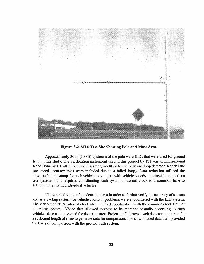
Figure 3-2. SH 6 Test Site Showing Pole and Mast Arm.

Approximately 30 m (100 ft) upstream of the pole were ILDs that were used for ground truth in this study. The verification instrument used in this project by TTI was an International Road Dynamics Traffic Counter/Classifier, modified to use only one loop detector in each lane (no speed accuracy tests were included due to a failed loop). Data reduction utilized the classifier's time stamp for each vehicle to compare with vehicle speeds and classifications from test systems. This required coordinating each system's internal clock to a common time to subsequently match individual vehicles.

TTI recorded video of the detection area in order to further verify the accuracy of sensors and as a backup system for vehicle counts if problems were encountered with the ILD system. The video recorder's internal clock also required coordination with the common clock time of other test systems. Video data allowed systems to be matched visually according to each vehicle's time as it traversed the detection area. Project staff allowed each detector to operate for a sufficient length of time to generate data for comparison. The downloaded data then provided the basis of comparison with the ground truth system.

23

The test process involved the simultaneous data collection, for vehicle counts in two lanes of traffic, using five detectors. Simultaneous testing is necessary to minimize differences in test conditions across all test devices. The detectors used in the test were the Accuwave 150LX Presence Detector, Nestor Traffic Vision video image detection system, Siemens PIR-1 series Passive Infrared Detector, the Remote Traffic Microwave Sensor (RTMS), and the SmartSonic passive acoustic Traffic Surveillance System.

The process of using time stamps to match vehicles subsequent to the data collection became a difficulty in the testing due to time drift within each system. Research staff spent substantial effort developing a system that was reliable. For that reason, much of the early data collected in these field tests was not deemed sufficiently reliable for this report. Only the most recent data are included in this report. Appendix B contains the graphic results representing test results from College Station. It includes plots of data in three formats: 1) raw counts of test system versus ILD system by 15-minute counts, 2) percent error of test system compared to the loop system counts for each hour, and 3) raw data plots of both loop and test systems by 15-minute intervals for visual comparison. These graphics indicate some time periods during the test days when comparisons were not made. In most cases, part of the field system was off-line for repairs or had malfunctioned. Other specifics are noted below in the Results section for each detector.

These tests utilized a single ILD in each lane connected to an International Road Dynamics classifier for vehicle count verification. This classifier had been previously ground truthed and was used along with time stamped video recordings for vehicle count verification for all detectors. The Accuwave, PIR-1, and RTMS acquired lane count data using a National Instruments digital IO data acquisition card installed in an Industrial Pentium computer. The research team wrote four virtual instruments (Vis) with Lab View software to collect the data through the data acquisition card's optically isolated inputs. The Vis running in Lab View time stamped each vehicle detection and wrote the time in military format to a text file for each vehicle detection. In order to acquire accurate data that could be compared at a later time, the three computer clocks, the classifier, and the video recorder clocks had to remain synchronized. However, the various clocks would drift apart by several seconds in a 24-hour period. Each day,

researchers synchronized all the clocks before beginning data collection and checked them three or four times a day for time drift.

3.3.1 Accuwave lSOLX Presence Detector

3.3.1.J Accuwave Introduction

The Accuwave Presence Detector model 150LX is a microwave sensor that can detect a range of vehicles in different environmental conditions. According to the vendor, the detector will perform the same in both sidefire and head-on applications. For optimum performance, the detector location should be selected to maximize the return signal from detected vehicles, while minimizing extraneous reflected signals. The detector has adjustable operating parameters that

24

may be downloaded by the user using the setup program and interface. The Accuwave operates by characterizing the received signal to form a basis for detection and indicates changes to this received signal. Low-level microwave radiation is partially absorbed and partially reflected by objects in the field of illumination. Objects may be tuned out of the signals as long as they are stationary, i.e., a pole, but anything moving in the field of illumination may require operating the detector at reduced sensitivity, or may require relocation of the detector for reliable operation.

3.3.1.2 Accuwave Setup

After the Accuwave 150LX Presence Detector was installed, it failed to tune and start detecting vehicles. An early problem was a defective serial communication selection switch, which required returning the 150LX for repair. Upon reinstallation, it was determined that the cable had to have individually shielded wire pairs for the detector to function properly. Beyond these two problems, the Accuwave stopped working during heavy rain and did not retune itself until the rain subsided. Table 3-2 is a summary of problems encountered with the Accuwave detection system.

Table 3-2. Accuwave Setup Events.

Date Problem Description Result

6125 Not operating after installation Checked with the installer

7/13 Not detecting and not retuning Sent interlace to installer for repair automatically

7/20 Not collecting vehicle detection data Wrote Lab View Program, wired to DAQ PC board

8/17 Not retuning automatically Naztec replaced cable detector and interface

3.3.1.3 Accuwave Results

TTI tested the Accuwave's detection accuracy on SH 6 even though it is designed for signalized intersections. TfI experienced two challenges in these tests. The first challenge was establishing an appropriate orientation of the detector in an attempt to capture only one lane. The research team was forced to orient the detector to count both lanes and then modify the count results when vehicles in the right lane and left lane were time stamped with the same time (based on output from other detectors). The second problem concerned the sampling rate used by the National Instruments setup. Field engineers varied the sampling rate between 350 msec and 450 rnsec to test its effect, and this almost certainly affected accuracy.

Field results show that the Accuwave count accuracy is affected by rain, as indicated by results provided in Appendix B. During August 21, 1998, field testing the Accuwave experienced continuous detections due to moderate to heavy rain, so results were not accurate.

25

On other dates during which there was no rain, the Accuwave counts during midday were usually within 10 percent of ILD counts. However, during other times, its error was in the 30 to 40 percent range.

3.3.1.4 Accuwave Conclusions

The Accuwave rain problem is significant for central and east Texas. For traffic signal applications, the observed problem would cause the detector to send a continuous call to the controller whether vehicular demand actually exists or not. According to the vendor, the detector will retune itself after the rain subsides. TTI found this to be accurate after replacing the original cable with one in which all pairs were individually shielded. The detector should be tested at an intersection to better assess its accuracy for that application.

3.3.2 Nestor Traffic Vision Video Detector

3.3.2.1 Nestor Introduction

The Nestor Intelligent Sensor's Traffic Vision is a video detection system using computer hardware and software for pattern recognition based on neural networks programmed intelligence that sees and recognizes images. Traffic Vision systems, powered by Nestor neural networks and the Nl4000 Recognition Accelerator chip, appear to have the potential to provide freeway information not currently available in competing systems. Traffic Vision can be used for a wide range of applications, including intersection control, highway monitoring, tollways, rail crossings, road and traffic studies, and community planning. According to the vendor, it provides more than 12 types of data ranging from vehicle counts and speeds to lane changes and occupancy to vehicle classification.

3.3.2.2 Nestor Setup

The Nestor Intelligent Sensor computer required a cooling unit for its central processing unit to operate without damage in the hot Texas summer environment. The cooling unit housed the entire Nestor central processing unit, and both went inside the cabinet. Because the cooling unit generated its own heat, project staff were forced to add fans inside the cabinet. Without the fans, the Nestor computer could only run with the cabinet door open. Initially, two fans were not enough to keep the internal cabinet temperature below 120 degrees Fahrenheit, so another fan was added. Once the temperature problem was solved, researchers noticed that the Nestor computer clock was drifting approximately five seconds per hour. This amount of time drift did not allow accurate comparison of the system with other detectors. Nestor engineers proposed trying a different Traffic Vision program to reduce the clock drift, but the problem continued. The solution was a time reference card installed in the computer's motherboard to keep the

system clock from drifting. Installing the time reference card required moving the Nestor card to a different slot in the motherboard; but that change caused the Nestor card to quit working. Nestor promptly sent another card and configured it from their home office using a modem and

26

PCAnywhere software. TTI personnel then powered up the unit and programmed it to start collecting traffic data. Nestor mpresentatives were very helpful and knowledgeable about their equipment. Table 3-3 is a summary of events encountered with the Nestor system during these tests.

T bl 3 3 N a e - . estor St E ts e up ven . Date Problem Description Result

7116 No cooling fans for cabinet Cannot leave running; fans ordered 7 /10/98

8/3 Unit shuts down from high temperature Added extra fan and increased ventilation

8/8 Unit shuts down for no apparent reason Sent log files to Nestor; connected modem

8/9 Unit shuts down for no apparent reason Nestor techs used modem to check CPU

8/10 Clock drifted five seconds per hour Installed new TVS executable file

8/11 Clock still drifting two seconds per Installed time reference card hour

8/12 Nestor card quit working after moving Nestor trying to diagnose card via modem

8/17 1 down waiting on new Nestor card Installed card and returned PC to field

3.3.2.3 Nestor Results

Nestor count accuracy was compared to the ILD counts. The Nestor overcounted on August 20 from 9:30 p.m. through 10:45 p.m. by as much as 20 to 30 percent. Sunset occurred at approximately 8:00 p.m., so the time period in question occurred after the daylight to dark transition period. The overcount was in both lanes. On this date, the Nestor continued to overcount until 6:30 a.m. In six out of seven nights, the Nestor consistently overcounted traffic volumes from midnight to 5:00 a.m. by as much as 40 to 50 percent. Other problem times were around 8:00 a.m. and 6:00 p.m. due to sun angles causing glare and shadows. These problems resulted in undercounts in the range of 10 to 40 percent. During other periods, the Nestor counts were typically within 5 to 10 percent of loop counts.

There was a short period of heavy rain during the field tests when the Nestor system was collecting data. This occurred on August 21 from 3:30 p.m. to 4:00 p.m. and beginning again at 7:00 p.m. for a few minutes. Rain was intermittent during other time periods as well. Nestor comparisons with ILD counts indicated undercounts during the periods of heaviest rain in the range of 6 to 8 percent. The 15-minute interval beginning at 5:00 p.m. indicated an undercount of 5 percent. These counts were not significantly worse than other non-rain count periods during the day. However, the Nestor changed from undercounting to overcounting at 8:00 p.m. that evening and continued until 11 :30 p.m. for all except one 15-minute period. The magnitude of the overcounts varied from 4 to 23 percent.

27

3.3.2.4. Nestor Conclusions

. The most consistent errors generated by the Nestor system were midnight to 5:00 a.m.

and near 8:00 a.m. and 6:00 p.m. The magnitude of the errors were much larger than anticipated, given that traffic volumes were relatively light during almost all count intervals.

3.3.3 PIR~l Passive Infrared Detector

3.3.3.l PIR-1 Introduction

The PIR-1 series Passive Infrared Detector (PIR-1) is from Eagle Traffic Control Systems, a subsidiary of Siemens Energy and Automation. The PIR-1 detector can be used for static and dynamic detection of vehicles. The PIR detection technology is based on the fact that all objects above absolute zero emit heat radiation in the remote infrared range of the electromagnetic spectrum. This technology reacts only to movements in or through the active zones. Slow changes in background temperature, caused by changing weather conditions, are not evaluated. In order for the detector to function properly it should be mounted to a stable structure and correctly aligned. The viewing direction for all detection zones must be unobstructed.

3.3.3.2 PIR-1 Setup

The PIR-1 detector generates an AC output signal for detection purposes so the output signal had to be modified for this test. Project staff used a National Instruments data acquisition board which required a DC input voltage. Also, the 60 Hz AC output signal operated on very low power so project staff designed a circuit that allowed use of a data acquisition board. The first stage of the interface circuit, depicted in Figure 3-3, contained an input buffer with very high input impedance. The high input impedance kept the input signal from attenuating. The next stage is an inverting amplifier with a gain of R2/R1• The purpose of the gain is to increase the voltage to a level high enough for the data acquisition board to use. The next stage was a full wave rectifier to convert the AC voltage into DC voltage. The capacitor is used in the circuit to filter out variations in rectifier output voltage. Researchers had to consult with Eagle Traffic Control Systems to make the PIR-1 detect only one lane. In its original mounting location on the pole, the PIR-1 could not be orientated to count only one lane. Therefore, it had to be moved from the pole to the mast arm. The horizontal angle between the detector and the road had to be 45 degrees or less to detect only one lane of traffic. Table 3-4 is a list of events associated with testing the PIR-1 detector.

3.3.3.3 PIR-1 Results

The PIR-1 error rate (compared to lane 1 loop counts) was consistently largest from midnight to 5:00 a.m. and reached magnitudes in the 20 to 50 percent range. The detector undercounted in one of six data sets recorded for this time period and substantially overcounted on four of the six. During daylight hours, the detector was within 10 percent of baseline loops

28

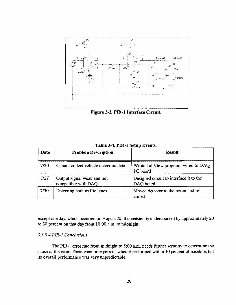
·y3 V'/

r:1r:

0Hl4DD2

RL

550 ohm

Figure 3-3. PIR-1 Interface Circuit.

T bl 3 4 PIR 1 S t E ts a e - . - e up ven .

Date Problem Description Result

7/20 Cannot collect vehicle detection data Wrote Lab View program, wired to DAQ PC board

7/27 Output signal weak and not Designed circuit to interface it to the compatible with DAQ DAQboard

7/30 Detecting both traffic lanes Moved detector to the boom and re-aimed

except one day, which occurred on August 20. It consistently undercounted by approximately 20 to 30 percent on that day from 10:00 a.m. to midnight.

3.3.3.4 PIR-1 Conclusions

The PIR-1 error rate from midnight to 5:00 a.m. needs further scrutiny to determine the cause of the error. There were time periods when it performed within 10 percent of baseline, but its overall performance was very unpredictable.

29

3.3.4 RTMS Detector

3.3.4.1 RTMS Introduction

The RTMS (Remote Traffic Microwave Sensor), is a self-contained microwave sensor that detects and monitors road traffic. It is designed to serve in applications of highway traffic management and intersection control. The RTMS is a true-presence detector that can provide presence indication as well as volume, lane-occupancy, speed, headway, and classification information in up to eight discrete detection zones. The information is provided to existing controllers by contact closures and to other systems by serial communications lines. The detector can be mounted forward for single lane detection or sidefire for multiple detection zones. The mode of operation is configured with the setup program using a computer and serial communication.

3.3.4.2 RTMS Setup

The RTMS initially had similar internal clock problems as experienced with the other detectors. The RTMS setup program software would record individual vehicle lane counts, but the software would not start recording its 60-second vehicle count at a consistent point in time. The researchers upgraded the software, but the problem continued. For this test of the RTMS, the separate input signals for detecting lanes one and two came from a 15V DC power supply. The power supply voltage was switched on and off with the two optically isolated contacts in the RTMS for lanes one and two. TTI researchers connected a shielded two-pair wire from the data acquisition card's optically isolated inputs to the connector plug on the RTMS. Connecting the wire to the military type plug required ordering special pins from the vendor. Table 3-5 is a list of events associated with the RTMS detector.

Table 3-5. RTMS Setup Events.

Date Problem Description Result

8/10 All vehicle counts cannot be taken at the Install latest version of the software same time

8/11 All vehicle counts cannot be taken at the Cannot verify data with classifier same time

8/13 Cannot collect accurate data Ordered pins for plug, ran wire for contact switches

8/15 Waitin£ on pins to come in from EIS Wrote Lab View programs for each lane

8tr •t collect data Installed pins and wired to DAQ PC board

30

3.3.4.3 RTMS Results

The RTMS counts were compared against aggregated loop counts from lanes 1 and 2. The combined counts plotted in Appendix B indicate results that are very consistent with ILD counts during most of the nine-day count period. Its count accuracy is also very consistent at all count levels, even though the highest flow rate was only 1,800 vehicles per hour for the two lanes combined. Its largest discrepancy with loop counts occurred on August 21 at 3:00 a.m. with a count error of 15 percent. The 3:00 a.m. and 4:00 a.m. count intervals on other days also reflect overcounts, but always 10 percent or less.

3.3.4.4 RTMS Conclusions

The RTMS was the most consistently accurate detector tested in these field tests. Reasons for its higher error rate for the 3:00 a.m. and 4:00 a.m. periods should be further scrutinized in other field tests to determine the cause. It should be tested on a high-volume freeway as well as at signalized intersections to further evaluate its accuracy.

3.3.S SmartSonic Acom;tic Detector

3.3.5. l SmartSonic Introduction

The SmartSonic Traffic Surveillance System is a passive acoustic highway sensor capable of providing vehicle presence and speed. Each sensor has a single detection zone and is composed of a microphone array that listens to sound energy emitted from vehicles. The detection zone size and shape are determined by the sensor installation geometry. When a vehicle enters the detection zone, an increase in sound energy is detected, and a presence signal is generated. When the vehicle leaves the detection zone, the sound energy drops below the detection threshold, and the presence signal becomes inactive.

3.3.5.2 SmartSonic Setup

One problem with the SmartSonic System was that the lane one detector sometimes detected both lanes. This problem was solved by a simple aim adjustment, turning it away from lane 2. Another minor problem with the SmartSonic was that the internal clock drifted approximately four seconds in 24 hours, requiring adjustment with each day's data collection.

3.3.5.3 SmartSonic Results

The SmartSonic showed no bias toward being more accurate at low volumes versus higher volumes. However, the SmartSonic usually overcounted vehicles between midnight and 6:00 a.m. The error rate was as much as 50 percent higher than loop counts on six out of seven of the days when count data were available. On the undercount day, the magnitude of error was 35 to 50 percent during those same hours. Midday accuracy for the SmartSonic was usually within 5 percent of loop counts.

31

3.3.5.4 SmartSonic Conclusions

The SmartSonic exhibited a much higher error rate between midnight and 6:00 a.m. than during other periods of the test days.

3.3.6 Tests on High-Volume Freeways

The SH 6 tests were intended to be preliminary testing which would be followed by more rigorous testing on a high-volume freeway. These additional tests occurred in Houston and Ft. Worth. One of the initial challenges was finding suitable sites. Criteria included sites with functional loops within 30.5 m ( 100 ft) from the pole used to support cameras or other test system components, two loops in each lane for speed studies, good line of sight from camera to loops, tangent roadway, nearly flat profile, and a 12.2 m (40 ft) pole within 4.6 m (15 ft) of the nearest travel lane. It should be noted that VIDS performance is even better with cameras located closer to the monitored lanes or directly over the lanes. However, TxDOT does not typically mount freeway cameras over the lanes, so the minimum separation is anticipated to include the shoulder width, the thickness of a barrier system, and possibly an additional distance to separate the barrier from the pole. The other possibility is to p1ace a mast arm on the pole to move the camera closer to the lanes. For speed verification, each lane must have two loops instead of just one. The location should also have minimal weaving and lane changing. Both of the high-volume sites discussed below had only single loops in each lane, and the Houston loops were too far away from the pole.

3.3.6.J Houston Field Tests

For field testing in Houston, TTI chose a location on eastbound US 290 near the Pinemont Drive overpass on the northwest side of the city. The test section is a six-lane freeway with an HOV lane in the center. The site had single ILDs in each lane located approximately 150 m (500 ft) downstream of the camera pole in all three eastbound main lanes (the HOV was not part of the test). The site had a 12.2 m (40 ft) surveillance camera pole 7.6 m (25 ft) from the right lane of the freeway. The three systems tested at this site were the RTMS detector and two video image detection systems-the Nestor Corporation's Traffic Vision and the Autoscope 2004.

TTI initially attempted to use the TxDOT surveillance camera feed from the field site by placing video image processors in the Houston TranStar building for video input to the Nestor and Autoscope processors. TTI researchers installed the Nestor and Autoscope computers in the TranStar building and configured them for the three lanes of eastbound traffic on US 290. The RTMS position was on the camera pole at a height of 5.2 m (17 ft) from the road surface. The data collection plan utilized an IRD TCC 500 classifier-counter connected to the three single ILDs near the pole. There were problems with this setup. First, the camera pan-tilt unit did not stay locked as TTI requested, requiring the Autoscope and Nestor to be reconfigured when the camera was moved. Second, the automatic iris of the TxDOT surveillance camera would not open sufficiently at night for the video detectors to work properly. Third, if the data storage time interval was less than 10 minutes, the RTC (RTMS data storage unit) did not have enough

32

memory to store per-lane vehicle data. Finally, keeping the RTC clock synchronized with the other computers was a problem.

The type and quality of the camera for a VIDS determines the accuracy of the system. For example, a monochrome camera is 10 times more sensitive to light than a color camera, so for low light levels and at night, monochrome cameras perform better and have higher resolution than color cameras. Without an automatic iris in the camera lens, changing ambient light conditions could cause the camera's output to the VIDS to be useless. Also, an infrared filter on the camera lens reduces glare from the sun and headlights at night, thereby increasing detection accuracy.

Installing a TTI camera on the pole and positioning an equipment trailer at the base of the pole to store computers for the Autoscope, Nestor, and RTMS solved these problems. With the support of a TxDOT bucket truck, TTI installed the camera on the pole 1.5 m (5 ft) below the surveillance camera. TTI used a time-lapse VCR in the trailer in addition to the three computers. TTI personnel then networked the three computers and started a program to keep all the PC clocks synchronized. Even then, the Autoscope and Nestor systems were still not working properly at night. Upon review of the videotape, it became apparent that the camera was drifting out of focus at night. After adjusting the back focus on the camera to correct the problem, researchers reconfigured the Autoscope and Nestor for the three eastbound lanes, synchronized all the clocks, and began data collection.

TTI collected simultaneous data from the classifier-counter, Nestor, Autoscope, and RTMS for six consecutive days from the Houston site. The data analysis process accumulated all one-minute interval per-lane vehicle counts from all detectors to create 15-minute intervals, then copied these to an Excel spreadsheet. The analysis concluded with individual lane and total directional vehicle count comparisons between loop values and test system values. Appendix C shows these results by travel lane.

All three of the devices tested in Houston had greater errors during very low volume time periods (generally, the early morning hours). It is recognized that these higher errors result primarily from smaller counts within each count period, which exaggerate the apparent differences between baseline results and test results. A quick observation of the raw count plots shown in Appendix C clearly indicate close agreement of test systems during low volume time periods. Given this phenomenon, the following comparisons focus on higher volume time periods, which begin at approximately 6:00 a.m. and continue until midnight.

The Autoscope results were adversely affected by the pole offset and other camera factors. Future testing will attempt to address these factors by finding a better pole location and making camera adjustments. Lane 1 Autoscope counts from 6:00 a.m. to midnight during the five-day test period (February 9 through February 13, 1999) were generally within 10 percent of baseline counts. Many of the 15-minute counts were within 5 percent. Counts after darkness were the exception, with the Autoscope overcounting by as much as 30 to 40 percent. The lane

33

1 counts should have been the most accurate of the three lanes, and a better camera and an improved position closer to the lane should improve its accuracy. Lane 2 counts were more erratic than lane 1 counts. Daylight errors were both positive and negative in the range of plus 20 percent to minus 50 percent. Nighttime errors were even worse. Lane 3 daylight errors were in the plus 20 to minus 30 percent range, and nighttime errors were again worse.

The Nestor both overcounted and undercounted in lane 1 by 30 percent during daylight hours. There were many time periods during the daytime when its count error was in the zero to 10 percent range. Its lane 2 and lane 3 count errors are not as disparate from lane 1 errors as the range found with the Autoscope. Again, a better camera and camera position would probably improve these results.

The RTMS was apparently not affected by changing light conditions as were the two VIDS units. Therefore, the RTMS count performance during early morning and late afternoon light transition periods was similar to its mid-day performance. The RTMS generally undercounted lane 1 traffic by 5 to 10 percent during the test period. In lane 2, the RTMS mostly overcounted in the range of up to 10 percent. On two days, it also undercounted traffic in lane 2 but usually hy no more than 5 percent. Lane 3 counts showed no bias toward overcounting or undercounting for most time periods, with errors in the range of 10 percent. RTMS performance was unaffected by the distance of the pole from the roadway.

3.3.6.2 Ft. Worth Field Tests

The research team selected a site in Ft. Worth on IH-20 at Hartman Road. This 10-lane portion of IH-20 consisted of an overpass above Hartman, which is a two-lane road. Both sides of the freeway had ILDs but the westbound side had loops located near the camera pole. The right lane of westbound IH-20 was an auxiliary lane with an entrance ramp approximately 0.3 km (1000 ft) upstream from the site and an exit ramp approximately 0.3 km (1000 ft) downstream. This site was also selected because the single Il.Ds were working in all five lanes and were located only about 22.9 m (75 ft) downstream from the camera pole. The 18.3 m (60 ft) camera pole was offset 4.6 m (15 ft) from the right lane as measured horizontally, with the road surface 5.2 m (17 ft) higher than the base of the pole. These field tests included four systems operating simultaneously-the Autoscope 2004, Nestor TrafficVision, RTMS, and the SAS-1 acoustic detector by SmarTek. Paradigm mounted the Autoscope camera 11.0 m (36 ft) from the road surface just below the TxDOT surveillance camera and aimed it in an easterly direction toward oncoming traffic. Then, the camera was rotated 90 degrees counterclockwise on its major axis to improve its performance. The Nestor used the surveillance camera at the top of the pole for video input. TTI installed the SmarTek acoustic detector on the camera pole at a height of 7.9 m (26 ft) above the roadway. The RTMS was mounted on the same pole at 5.2 m (17 ft) above the road surface. No performance results are provided from these tests due to the lack of credible baseline data, as discussed in Section 3.2.1.5.

34

3.3.7 Overall Field Test Conclusions

The consistency of the error across all non-intrusive detectors during low-volume periods late at night suggests that the percent error considerations need to be supplemented with another comparison, such as raw counts. The primary reason these percent errors are higher in magnitude than during other time periods is the small number of vehicles involved. Appendix Craw data plots indicate that the absolute differences across all detectors during low volume time periods late at night compared to ILDs was very small. Detectors tested both in College Station and in Houston demonstrated generally lower percent errors and more consistent operations in the lower demand environment in College Station.

3.3.8 Experience of RCOC with Autoscope

The Road Commission of Oakland County (RCOC), Michigan, represents one of the largest field tests of video detection and other ITS equipment in the United States. This program began installing Autoscope video detection equipment for signal control in 1991 and, in August 1998, was operating 272 video processors and approximately 1,090 cameras. The overall program is called FAST-TRAC (Faster and Safer Travel-Traffic Routing and Advanced Control). The RCOC is not involved in freeway operations.

3.3.8.J Camera Mounting Considerations

The typical location of RCOC cameras is 1 m (3 ft) off the roadway, because the camera is mounted just behind the curb to allow a slight longitudinal angle for shadow processing. Because RCOC uses SCA TS, it needs to have the camera pointing down at a very steep angle. SCA TS counts vehicles and measures the length of the vehicle and time it is within the detector.

Typical camera heights are between 9.1 m and 13.7 m (30 ft and 45 ft), although recent installations are between 11.6 m and 13.7 m (38 ft to 45 ft). Focal lengths are now almost exclusively 4.8 mm. RCOC started with some 6 mm, which had a sharper picture, but otherwise did not work as well. In some cases, there may be a left-tum lane where a vehicle would stop beyond the stop bar and be outside the detection zone.

The maximum number of lanes for a single camera without significant occlusion is three. Taller vehicles mask smaller vehicles or get counted in the adjacent lane. So, RCOC rarely covers more than three lanes with each camera. For example, one site may include three through lanes, a right-tum lane, and a dual left, which would be covered by two cameras. The three through lanes and right-tum lane would be covered with one camera mounted over the right-hand curb. The other camera, mounted on the left side, covers the two left-tum lanes.

An improvement that Autoscope has developed is a directional detector. With this, if a vehicle encroaches into an opposing lane, for example, it will not get detected and it does not generate the false calls it might otherwise.

35

3.3. 8.2 System Accuracy

The Autoscope has significant problems in thick fog and in snow. Also, in daylight, it cannot always differentiate between a vehicle and its shadow. However, the Auto scope system is much improved over earlier versions and is being equipped with a faster processor to improve its shadow processing. With the previous processor, other functions were compromised to process shadows. RCOC's current error rate due to shadows is in the range of 1 to 2 percent. In snow, the Autoscope (and any other video detection system) sees a white background, and individual tracks in the snow may confuse the system. The Autoscope does not miss vehicles as much as it overcounts (due to false calls). System operators do not think heavy rain is a problem. In cold weather months, the camera heater keeps the lens cover clear. Even in blowing snow, it clears the cover quickly.

Prior to purchasing and installing video detection equipment, RCOC's overall experience with loops was poor. Based on their experience, they knew that ILDs would not give the reliability needed to operate an adaptive signal control system. RCOC continues to use ILDs at only approximately 50 intersections.

Autoscope is sensitive to electrical storms, but so are ILDs. RCOC personnel predict that above ground systems will eventually replace ILDs, at least in the northern states. The freeze­thaw environment in those states precludes loop installation or repairs during three to five months of the year whereas RCOC makes Autoscope repairs year-round. Also, maintenance forces are either off the roadway or in the right lane only for the repairs, whereas loops would force repairs to be in the roadway. Autoscope repairs are generally one-half to one hour in length, whereas loop repairs take longer.

3.3.9 TxDOT Experience

A few of the mid-size and large urban areas in Texas have installed VIDS for either short-term tests or for permanent installations. Some of the urban areas represented are: Austin, Ft. Worth, Houston, Laredo, San Antonio, and Waco. Districts that have conducted their own tests do not usually have definitive test results to report, so the information from districts is limited.

The Ft. Worth district tested the Peek VideoTrak 900 in April 1997 on a freeway where ILDs were available to provide comparable counts and speeds. System accuracy was heavily dependent upon spending considerable time in set-up. Traffic counts were in error by approximately 15 percent prior to the "fine tuning." With the camera mounted at the outside edge of the freeway, there was occlusion on interior lanes and, therefore, more error. Accounting for this occlusion, the count accuracy was within 5 percent on the next two lanes during daylight and good weather with traffic approaching the camera.

36

The San Antonio district deployed two Autoscope systems for temporarily controlling traffic signals on frontage roads that "worked fairly well." Its accuracy was reported to be in the 85 to 90 percent range. The district also installed an Odetics system that is working well.

The Waco district has an Odetics video image detection system on Valley Mills Drive at five signalized intersections. Following an initial period of less than desired accuracy, the vendor made improvements that resulted in a 93 to 95 percent accuracy rate. The district verified this accuracy by using a monitor in the cabinet to receive video from the Odetics processor unit and watch for detections as they occurred in real time.

3.4 SUMMARY OF DETECTOR ACCURACY AND RELIABILITY

This chapter covered two key topics regarding vehicular detectors: accuracy and failure rates. Because ILDs are a mature technology, various jurisdictions were able to provide information on both accuracy and failure rates on ILDs. Accuracies of competing non-intrusive detectors can be established, but documentation on their failure rates is not well established. Tables 3-6 and 3-7 provide some of information about both categories of detectors.

Table 3-6. ILD Accuracy and Failure Rate.

TxDOT Dallas Houston Lufkin Odessa

Agency

San Antonio Tyler Yoakum

Research 0-1715

Cal trans

DOT

an ITS Center

FHW A (Hughes study)

FHW A (Minnesota study)

Europe Netherlands Switzerland

Accuracy

NA

-1.08% to +1.87%

NA

NA

NA

±1%

-1.0% to +1.4%

NA

37

Failure Rate

3-5%/yr 2%/yr 2%/yr 7%/yr

1-2%/yr 3%/yr 3%/yr

NA

50%

5%

2%

NA

NA

1per1,500 5 per 200

T bl 3 7 N I t a e .. on- n rus1ve D tect C tA e or oun ccuracy B d TTI F' Id T ts ase on 1e es . Detector Typical Percent Error

Midday Dark Weather/Mounting Problems

Accuwave 30% to40% 30% to40% Heavy rain causes continuous call; movement generates detection

Nestor -5% +10% to+40% Shadow/glare: -10% to -40%

PIR-1 plus/minus 10% +10% to +30% Possible weather-related problem

RTMS plus/minus 5% +10% None

SmartSonic plus/minus 5% up to 50% None

38

4.0 COST ANALYSIS OF VEHICLE DETECTION TECHNOLOGIES

4.1 INTRODUCTION

One of the most significant elements in the choice of detection technology is the life­cycle cost. The elements of life-cycle cost that need to be considered include: installation costs; maintenance costs; traffic control; motorist delay and related excess fuel consumption; additional pavement maintenance costs; and costs related to increased crash rates during installation and maintenance of some detectors. Some of these factors vary by intersection versus freeway, size of urban area, pavement type, and area of the state. For ILDs, installation costs on freeways may include longer runs from the loops to the cabinet as compared to intersections. Pavement cutting in concrete takes longer than in asphalt if depth and width of cut are the same. In the northern parts of the state, ice and snow may cause maintenance costs to be higher than areas to the south. Some TxDOT districts replace failed loops in concrete by simply "routing out" the old loop

wires and putting new wires back in their place instead of cutting new loops. This takes less time than cutting new loops and is, therefore, less expensive. In asphalt, districts typically replace failed loops by installing completely new installations. Exogenous factors, such as pavement condition and damage from other maintenance and construction activities, also cause variability in the costs of maintaining loops.

The following cost analysis utilizes cost data from several districts that represent different sizes of urban application and districts that had better than average documentation. Besides the general cost information from all districts, there is detailed information from three districts. The data from Houston, Waco, and Paris do not necessarily reflect costs that might be incurred in similarly sized urban areas, but their costs are, nonetheless, considered useful for other districts. The Houston district had cost data available for both freeways and intersections, whereas the other two only had intersection costs. The cost analysis first discusses ILD costs, followed by costs of other non-intrusive detection systems, and some of the variables affecting costs. Because of the many factors that affect the life-cycle costs of competing systems, it is recommended that TxDOT conduct site-specific cost comparisons.

4.2 TXDOT DISTRICT INDUCTIVE LOOP COSTS

ILD costs vary considerably across the districts. As an example, a 1.8 m by 1.8 m (6 ft by 6 ft) ILD and an arbitrarily selected conduit length of 52 m (170 ft) could cost in the range of $610 to $1,460. For an initial installation, one must add to this subtotal the cost of pull boxes, traffic control, loop detector amplifiers, and motorist delay. For intersections, the traffic control is often included in the bid price for saw cutting the pavement. For freeways, both traffic control and motorist delay represent a significant increase in loop installation and repair costs. Traffic control for a single lane closure can be $1,000 to $1,500 in large urban areas.

39

4.2.1 Houston Inductive Loop Costs

The Houston district maintains ILDs at signalized intersections as well as on freeways. Costs are significantly different for the two applications due to the traffic volumes involved and the resulting motorist delay and fuel differences plus the traffic control costs. The following sections describe the costs for each application.

4.2.1.l Houston Signalized Intersection Inductive Loop Costs

The Houston district also supplied information related to ILD replacements at signalized intersections that could be used to calculate periodic maintenance costs. The number of failures discovered over a time period of 10 years is shown in Table 4-1. There were as few as 42 loop failures discovered in a year's time and as many as 341 loop failures discovered in the 600 plus signalized intersections under TxDOT jurisdiction. It should be noted that other loop malfunctions required technicians to travel to the intersections that are not reflected in the table.

T bl 4 1 R l a e - . ep acemen t C t t F ·1 d L OS or a1 e oops a t I te t• . th H t n· t "ct. n rsec 1onsm e ODS on IS n

No.ILD Saw Cut No.of

Year Failures Meters (Feet) Intersections Discovered Maintained

1989 42 1395 (4576) 608

1990 271 7255 (23796) 669

1991 195 4927 (16161) 704

1992 211 5354 (17561) 741

1993 177 4354 (14281) I 759

1994 84 r-1338 (4389) ' 770

1995 208 4866 (15960) 802

1996 314b 11256 (36920) 848

1997 341 7650 (25092) 932

1998 1::\1 7375 (24190) c 1,006

a Costs exclude motorist delay and excess fuel costs. b Approximated from actual counts through June 1996. c Through July 1998.

40

Replacement Cost per Cost+TC Intersection a

$65,100 $107.07

$420,050 $627.88

$302,250 29.33

$327,050 I $441.36

$274,350 $361.46

$130,200 $169.09

$322,400 $402.00

$243,350 $286.97

$169,807 $182.20

$165,490 $164.50

In quantifying failure rates at the Houston intersections over a time period of several years, one must realize that some variables are difficult to quantify. The district has changed its loop policy and equipment over that time period. Because TxDOT provided the actual length of saw cut needed to replace failed loops, some of these changes will not significantly compromise the accuracy of cost calculations. However, the fact that some of the intersections were not traffic actuated (had no detectors) until recently is a source of error. The estimate of the cost per intersection will be on the low side because it assumes that all of the intersections had loops, that 100 percent of loop failures were discovered, and that no maintenance costs besides replacements were incurred. The resulting mean value of annual loop replacement cost per intersection is $335. Because of the conservative nature of this estimate, it is increased to $400 per intersection per year for further analysis.

The initial cost of a signalized intersection in Houston varies considerably. For later comparison with costs of competing systems, a "typical" intersection is hypothesized which has two-lane approaches and single left-tum bays in all four directions. Loops at the stop bar are 1.8 m by 12.2 m (6 ft by 40 ft) and set-back loops are 1.8 m by 1.8 m (6 ft by 6 ft). The main street speed limit is 65 km/h (40 mph), and minor street speed limit is 50 km/h (30 mph). Traffic control is included in other items in Houston bid prices'. however, delay/excess fuel costs are not included. The total cost of this intersection using current average bid prices for Houston is $22,200. Adding the annual maintenance figure calculated above, assuming a 10-year life for loops, and using a 5 percent rate of return, the annualized cost for this intersection is $3,275.

4.2.1.2 Houston Freeway Inductive Loop Costs

In Houston, replacement costs for loop wire in concrete include materials cost for wire, sealant, and so forth. This cost per unit of saw cut is lower than for the initial installation because the contractor simply cleans out the old saw cuts, so this process is much faster than cutting concrete for the first time. Therefore, the linear cost includes both the removal of the old loop and installation of the new loop wire and sealant. These repairs typically do not require installing new leads from the pull box to the controller. An important difference in the installation procedure between Houston and some other districts is that Houston uses a product called "detecta-duct" in the saw cut. It requires the cut to be wider, possibly increasing the price. However, durability should be increased, thereby reducing the life cycle cost of these sensors. If a loop fails in asphalt, the Houston district requires a new loop beside the old one.

A typical layout for pull boxes on freeways is one small pull box beside the loops, then another one close to the controller cabinet. The typical maximum distance between pull boxes is 91.5 to 122.0 m (300 to 400 ft) to make the wire pulls easier. The district uses two loops per lane for speed detection on freeway mainlanes and also on frontage roads for ramp metering. The bid item is based on the length of saw cut, so there are only two wires in the cut except in the loop itself where there are three. For calculating traffic control costs, the Houston district currently requires lane closures at night for loop repairs and other freeway maintenance. In some cases, the freeway is closed, and traffic is routed onto frontage roads. This factor creates a significant cost difference between freeways and intersections.

41

Table 4-2 summarizes estimated installation and replacement ILD costs for both directions of a six-lane freeway which has concrete pavement, 3.05 m (10 ft) paved shoulders, 3.66 m (12 ft) lanes, requiring two pull boxes with one pull box near the loop site and one near the cabinet. A six-lane freeway facilitates comparison with video image detection systems as discussed later in this report. Each lane has two 1.8 m by 1.8 m (6 ft by 6 ft) loops spaced 3.66 m (12 ft) apart.

T bl 4 2 C t f In tall f a e . . OS 0 s a mn an dR I t fH t Fr ep acemen o ous on eeway Lo ops.

INSTALLATION COST ITEM (12 Loops) COST

Saw cut: 49.6 ft x 12 x $6.60/ft a $ 3,931.00 Lead in from shoulder to pull box: Conduit: 24 ft x $7 .25/ft 174.00 Wire (included above)

Bore (158 ft x $12.15/ft) 1,920.00 Pull boxes ($408 ea. x 4 1,632.00 Lead in from pull box to pull box Conduit: 157 ft x 2 x $7 .26/ft 2,280.00 Wire (2 conductor shielded): 157 ft x 12 x 2 x $0.15/ft 565.00 Pull box to cabinet: 15 ft x 12 x 2 x $0.15/ft 54.00 Loop detector 1080.00

Traffic control 6,000.00 Motorist delay b 10,000.00

TOT AL INSTALLATION COST $ 27,636.00

Installation cost per loop $ 2,303.00

REPAIR COST ITEM (per loop)

Saw cut: 50 ft x $6.56/ft $ 328.00 Traffic control 1,500.00 Motorist delay c 5,000.00

TOT AL REPAIR COST (per loop) $6,828.00

a Note: If power header is used, add additional saw cut and loop wire. b Motorist delay for installation varied from $1,000 to $15,000, depending on the time period. c Motorist delay for repair varied from $200 to almost $15,000 depending on the time period.

Motorist delay costs are highly variable by time of day, and thorough evaluation requires several assumptions. Recent hourly traffic counts on a Houston freeway provided the basis of delay cost calculations. Because the Houston district now requires lane closures at night, delay costs are much less compared to daytime. However, motorist delay, even at night, is highly sensitive to the actual hours of operations and the number of lanes remaining open. Delay calculations used the QUEWZ program to calculate road user costs, assuming the freeway

42

remains open with a rmrnmum of one freeway lane in use. Delay costs varied from approximately $1,000 to approximately $15,000, depending on the time period when the work was done.

Using a motorist delay cost of $10,000 for the installation, the initial cost of 12 ILDs on a freeway would be $27 ,600, or $2,300 per loop. The total cost to replace a loop is just over $6,800 if traffic control cost and motorist delay amount to $1,500 and $5,000, respectively, for each replacement. Based on these initial and maintenance costs, a loop failure rate of 5 percent per year (system life of 20 years), the annualized cost of the six-lane freeway loop system would be $6,295. If motorist delay and excess fuel consumption is ignored for both installation and maintenance, the annualized cost for 5 percent and 10 percent failures per year would be $2,510 and $4,475, respectively.

4.2.2 Waco Inductive Loop Costs

The Waco district has an estimated 700 ILDs. This is based on 120 intersections that are signalized; 70 percent of the intersections are actuated, at an average of eight ILDs per intersection. For purposes of comparison with non-intrusive technologies later in this chapter, it is useful to compute the cost of installing an ILD system on Valley Mills Drive. By applying the most recent "average bid prices," one can calculate the cost of an ILD system for comparison with the cost of the Odetics system currently being used. To do so, the following factors are important: speed limit, intersection geometrics, number of driveways needing boring, and TxDOT specification for loop placement. A 75 km/h (45 mph) design speed requires three 1.8 m by 1.8 m (6 ft by 6 ft) loops in each lane at distances of 24 m (80 ft), 43 m (140 ft), and 67 m (220 ft) from the stop bar, plus a long loop at the stop bar. The current cost of saw cuts on the main street and side streets, conduit, wire, pull boxes, and boring for each of the five intersections along Valley Mills Drive would be $33,345 before adding the cost of traffic control and motorist delay. The expected life of a loop system in the Waco district is approximately seven years, according to district personnel. Ignoring the cost of traffic control and motorist delay, the annualized life-cycle cost would be $13,757.

4.2.3 Paris Inductive Loop Costs

The Paris district recently installed ILDs at two intersections that previously used fixed time control. The two intersections on the north and east sides of Paris involve US 82, Business 82, and US 271. The total number ofILDs installed at the US 82/Business 82 intersections was 14 each 1.8 m by 9.1 m (6 ft by 30 ft) with 1.8 m (6 ft) power header, and 22 each 1.8 m by 1.8 m (6 ft by 6 ft) loops. The intersection of US 82/US 271required14 each 1.8 m by 15.2 m (6 ft by 50 ft) loops with 1.8 m (6 ft) power headers, and 14 each 1.8 m by 1.8 m (6 ft by 6 ft) advance loops. The district provided traffic control, so its estimate was substantially lower than if they had hired a contractor to provide the services. The total initial cost of detection using ILDs for the US 82/US 271 intersections was $38,234; for the US 82/Business 82 intersection, the total initial cost was $39,560.

43

The Paris district of TxDOT also estimated loop replacement costs. Replacement of a 1.8 m by 6.1 m (6 ft by 20 ft) loop costs the district $507 .88, while a 1.8 m by 12.2 m (6 ft by 40 ft) replacement costs $885.13. Determining the annual cost made use of the district's estimate of failure rates and their replacement cost information. Failures were assumed to occur at a rate of 2 percent per year for the first five years, 4 percent per year over the next five years, and 7 percent per year over the final 10 years of an assumed 20-year system life. Life-cycle costs for either interchange will be very similar, so only the US 82/Business 82 interchange is used. It has a total of 39 loops installed, for a total replacement cost of $19,807. Converting the initial installation cost plus replacement cost to an annual cost at a 5 percent rate of return yields $4,055.

4.3 NON-INTRUSIVE DETECTION COSTS

4.3.1 Video Image Detection Systems

4.3.1.1 Out-of-State Cost Information

The Road Commission of Oakland County (RCOC), Michigan, currently represents the largest installation of video detection equipment in the United States. RCOC has documented costs of installation and maintenance of this equipment. Equipment prices have varied somewhat from one purchase to another, and prices vary for Autoscope processors based on the number of channels needed for a particular intersection. RCOC purchased 2-channel, 4-channel, and 6-channel units, depending on the geometric layout of the intersection. For recent procurements, the bid prices were $25,200 for the 2-channel, $20,175 for the 4-channel, and $36,175 for the 6-channel. According to RCOC personnel, the relatively low price for 4-channel units was due both to quantities purchased and a simplified specification. The cost of a camera plus line isolation units was approximately $2,500 per camera. The purpose of the line isolation unit is to improve the video signal. RCOC personnel do not believe that the Autoscope systems have any real competition at the present time, at least for the FAST-TRAC (Faster and Safer Travel-Traffic Routing and Advanced Control) application, so future costs may be less. Maintenance costs are covered in more detail below.

Costs were well documented by RCOC, which kept records on their FAST-TRAC system for the most recent years since beginning installation in 1991. Detailed information from R COC based on recent actual monthly expenditures provided the necessary information to determine the life cycle costs of these Autoscope systems. The information summarized in Table 4-3 represents a total of 194 Autoscope controllers and 692 cameras installed by RCOC. These are actual cost data for eight months in 1995, all of 1996 and 1997, and January through May 1998 for five suburban areas near Detroit, Michigan.

Table 4-3 costs include labor, fringe benefits, and equipment costs (e.g., repair truck and radio). Because the Autoscope systems were under warranty (for at least part of this time), cost of repair parts and new replacement units were paid for by the manufacturer or distributor. Therefore, for older units whose warranty period has expired, the maintenance cost could be

44

higher. Based on over three years of maintenance information, the monthly average cost per camera for maintenance ranged from a low of $2.02 to a high of $8.34; for Autoscope units, the range was $4.31 to $54.26. Using mean values, one could anticipate spending approximately $5.05 per month on camera maintenance and $26.71 per month on processor maintenance.

Table 4-3. Summary of Monthly Maintenance Costs of Four RCOC Systems. a

System Year Controller Camera

Auburn Hills 1995 b $868 $427 41 controllers 1996 568 413 139 cameras 1997 573 221

1998 c 177 845

Pontiac 1995 $384 $157 14 controllers 1996 2,336 266 48 cameras 1997 164 128

1998 44 0

Rochester Hills 1995 $714 $650 51 controllers 1996 561 414 187 cameras 1997 865 253

1998 594 199

Troy 1995 $1,725 $3,434 88 controllers 1996 6,031 1,480 298 cameras 1997 3,189 3,031

1998 22 353

OVERALL UNIT COSTS d 1995 $22.23 $8.34 194 controllers 1996 54.26 4.25 692 cameras 1997 26.04 5.61

1998 4.31 2.02

a Costs of monthly labor, fringe benefits, and equipment costs (truck, boom, radio). Equipment costs covered by manufacturer/distributor. Total of 19 jurisdictions have Autoscope equipment installed to date. b Monthly average January through August 1995. c Monthly average January through May 1998. d Total number of cameras and controllers shown for 1998; prior years are less.

4.3.1.2 TxDOT District Cost Information

The Waco Odetics VIDS on Valley Mills Drive cost the district $32,000 for the following items: cameras and lenses, installation, two workstations (one primary and one backup), a laptop computer, and system software. The vendor provided support beyond what was

45

actually expected, so this system was probably less expensive than would normally be expected. Prior to implementation, the district calculated the cost to be approximately the same for the VIDS as for a loop system.

4.3.2 Non-VIDS Detector Systems

The only substantial cost information available for non-VIDS detectors pertains to initial costs of equipment. Even this varies, in most cases, depending upon the number purchased at any given time. The initial unit price typically gets reduced with larger numbers purchased. For purposes of this comparison, quantities less than 10 are assumed. Other assumptions regarding failure rates and maintenance costs are based on limited information from TxDOT districts.

4.3.2.1 Accuwave Detector

Based on information from a Texas distributor, the cost of the detector is $900, but it also requires an interface panel that costs $150. Each panel will serve two detectors. The cable typically used is a six-pair individually shielded cable. A four-pair has sufficient wire, but the Beldon six-pair is more readily available. Its cost is approximately $3.30 per meter ($LOO per ft). According to the vendor, the life of the detector should be approximately five to 10 years. There are units that have been in operation in Texas for three years. There appears to be very little maintenance required for the Accuwave. Once the detector's sensitivity and delay functions have been set for a particular location, it might have to be readjusted once. The warranty period is one year. It can detect presence in two lanes, but detection for a left-tum lane alone is more difficult because its detection area is larger. The Waco district experience with its nine Accuwave sensors supports the information from the vendor regarding low maintenance requirements.

4.3.2.2 Passive Infrared Detector

The initial cost of the PIR-1 detector is $1, 100 and has experienced limited use in the U.S. It has been used in Europe for 10 years, but information on its maintenance requirements was not readily available. Table 4-4 provides initial cost, maintenance cost estimates, average expected life, and annual cost information on two detector systems field-tested by TTI for comparison. The Accuwave and PIR-1 have similar applications, so they are the only two included for this comparison. All annual cost estimates used a 5 percent rate of return.

4.3.2.3 RTMS Detector

The RTMS detector costs $3,300 per unit ($4,000 if a data storage unit is included). It can be very cost effective when used in a sidefire mode because it can monitor up to eight lanes when the lanes are within a 4.6 m to 61 m (15 ft to 200 ft) range. Other costs for the system include cables for $200, a modem for $600, and installation costs estimated at $200. The vendor claims that its product has a life expectancy of 10 years.

46

Table 4-4. Accuwave and PIR-1 Annual Costs.

Estimated Annual Estimated Life Detector Initial Cost Maintenance Cost Expectancy

(yrs)

Accuwave a $975 b $200 7

PIR-1 a $1,100 $200 7

a Non-directional detector, can detect one or possibly two lanes. b Interface costs additional $150, serves two detectors.

4.3.2.4 SmartSonic Acoustic Detector

Annual Cost

$386

$395

The cost for a one-lane system includes the sensor array at $1,450 and the controller card at a cost of $800 (accommodates up to four lanes), so a four-lane system costs $7,000 (also includes transmission module). The detector can be mounted as far as 7.6 m (25 ft) horizontally away from a traffic lane, according to the vendor, but it works best if mounted closer. Detection requires one detector per lane, with each controller accommodating up to four detectors.

4.4 COMPARISON OF ILD COSTS AND OTHER DETECTION COSTS

4.4.1 Literature Sources

Even though information available in the literature on detector costs was limited, it provided useful comparisons for Texas costs. For example, reference ( 18) compared the cost of an Autoscope system on a freeway against a loop system. In all scenarios investigated, the video image system cost less than the loop system. The installation was on a freeway where one of the two available lanes was closed for two hours to install loops. According to their simulation program, this resulted in delay and extra fuel costs to motorists of $164,000, making the VIDS alternative more attractive than loops. In reference ( 19 ), component costs were higher than those found in TxDOT practice. Their $49.20 per meter ($15 per ft) for saw cuts was approximately four times the unit cost in Texas.

4.4.2 Study 0-1715 Findings

In a comparison study such as this, there are numerous assumptions both for estimating ILD costs and for estimating non-intrusive detector costs. Maintenance costs for either system could vary significantly. For video maintenance costs, RCOC costs were the only reliable data found that were both credible and covered a substantial time period. The extreme heat in Texas might cause video costs to increase, although the amount is debatable. Of course, cost is not the only criterion used by decision makers. One reason RCOC chose a non-loop detection system was because loop repairs are impractical in the coldest winter months. The three case study districts of Houston, Waco, and Paris provide some ranges of costs that could be expected elsewhere.

47

4.4.2.1 Houston

The Houston district had useful freeway and intersection cost information on IIDs. Initial costs of a "typical" intersection with two approach lanes and one left-tum lane on each of the four directions is $22,200. Therefore, annualized life-cycle cost of the loop system is $3,278. A competing video system would require a four-channel processor and four cameras. Assuming poles are available, the initial system cost would include an estimated $500 per camera for installation, $200 for cables, $20, 175 for a four-channel processor, and $2,500 per camera. Using the annual maintenance cost (averaged from the RCOC system) of $5.05 per month per cameras and $26.71 per month for processors, the annualized life-cycle cost for a system with 10-year life would be $4,573.

For a six-lane freeway in Houston with dual (trap) loops in each lane, lLD installation costs $27 ,600, or $2,300 per loop. If motorist delay is ignored, the total cost drops to $17 ,600, or $1,470 per loop. The cost to replace a loop is $1,830 assuming negligible delay cost. Based on these initial and maintenance costs, the annualized cost of the six-lane freeway loop system with loop failure rates between 5 percent and 10 percent per year would be $2,510 to $4,475. If significant motorist delay cannot be avoided, the annualized cost for 5 percent and 10 percent annual failure rates is predicted to be $6,295 to $11,734. A competing video image processing system would consist of a two-channel processor and two cameras. Assuming poles are available for cameras, a processor cost of $25,200, cameras at $2,500 apiece, installation cost of $500 per camera, and cable cost of $200, the 10-year life cycle cost with RCOC maintenance costs would be $4,508. If the system lasts 15 years, its annualized cost would drop to $3,467. If poles must be installed (two poles at $5,000 each), the annualized 10-year cost would increase to $5,803.

4.4.2.2 Paris

The loop cost comparison in Paris consisted of a diamond interchange for which the district had recent accurate cost information. The district provided its own traffic control, substantially reducing costs. The total initial cost of detection using lLDs for the US 82/Business 82 intersection was $39,560. The total replacement cost of loops over their life is anticipated to be $19 ,807. The annualized life-cycle cost of the loop system will be $4,055.

The cost of VIDS for the Paris interchange could include either two processors and six cameras or one six-channel processor and six cameras. The latter option is selected as the less expensive system. Based on RCOC costs for a six-channel Autoscope and the related hardware, the initial system cost would include $36,175 for the processor and $2,500 per camera. Installation cost is assumed to be $500 per camera; cable cost is $300; and anticipated maintenance costs are $687.72 per year for the processor and six cameras (from RCOC). Assuming a 10-year system life and no purchase of poles, the resulting annualized life-cycle cost would be $7,742.

48

4.4.2.3 Waco

Waco represents an example where video costs are extremely low and loop costs are extremely high. Costs to the district include the initial system cost plus only a few repair components. Future costs may increase as warranty periods expire. Therefore, assuming $1,000 per year annual maintenance cost for the first five years and RCOC maintenance costs for years 6 through 10, the annualized total cost of the Odetics system would be $5,941. In contrast, using Waco district bid prices, an ILD system to replace the system on Valley Mills Drive would cost almost $167,000 for all five intersections This ignores traffic control costs and motorist delay and excess fuel usage, both of which would be significant. Total annualized costs of the loop system would be $13,757.

4.5 SUMMARY OF COST COMPARISONS

The cost comparison between VIDS and ILDs in the TxDOT Houston district indicates only modest differences in annualized life-cycle costs between the two systems. In many cases, motorist delay would be a significant factor and should be included in the comparisons as appropriate. The larger differences between ILDs and VIDS in the other two districts are thought to reflect abnormal conditions. In the Paris interchange example, the 6-channel processor substantially increased annualized costs for the VIDS system, whereas the zero-cost for traffic control on the ILD system increased the disparity even more. The Waco system reflects the opposite extreme: an abnormally low cost for VIDS and an abnormally high cost for ILDs. Table 4-5 summarizes these costs. In general, VIDS is cost effective in cases where one video camera can replace many loops, as in Waco. Video would also be cost effective on many high-volume urban freeways if significant motorist delay cannot be avoided. Annualized costs were very similar for the two systems for the hypothesized Houston signalized intersection, which had fewer loops to maintain than the Waco example.

Table 4-6 summarizes cost information for both a six-lane freeway with trap loops in each lane and an intersection with two through-lanes and one left-tum lane per approach. These are total costs for each freeway monitoring station or intersection (all four approaches). Detector life is assumed to be as follows: VIDS and ILD-10 years, RTMS-7 years, and SmartSonic-5 years. Motorist delay and excess fuel consumption due to installation/maintenance are assumed to be negligible. Installation costs are as follows: VIDS-$500 per camera, RTMS and SmartSonic-$200 per system. Table 4-7 summarizes costs per lane. The RTMS is the least expensive because one unit can monitor up to eight lanes (sidefire). These costs reflect two RTMS detectors at each freeway station, one per side. In some cases, only one detector per station will be needed for up to eight lanes. In tests conducted by TTI, RTMS performance on the far side of a freeway was sometimes limited by concrete median barriers. VIDS can realistically cover up to three lanes per camera, so per-lane costs are minimized when the total number of lanes are even-numbered multiples of three, such as six or 12. ILD costs per lane are relatively constant; however, in reality, their costs increase somewhat with number of lanes due to longer lead lengths. Therefore, loops are generally the most expensive detector on freeways (and they are even more expensive if motorist delay and excess fuel consumption are included).

49

Table 4-5. TxDOT ILD Costs Com ared to VIDS Costs.

District Location Cost VIDS Annualized Cost

Houston Intersection $3,278 $3,370

Freeway $4,475a $4,443 b

Paris Interchange $4,055 $7,742

Waco Intersection $13,757 c $5,941c 11 Assumes 10 percent annual failure rate and ignores motorist delay, $6,295 with delay. b Cost increases to $6,515 if installation of poles required. c Cost per intersection.

T bl 4 6 D t t A a e - . e ec or r dT talC tC nnua 1ze 0 OS ompansons.

Annual Expected Annualized Detector Location Initial Cost Maintenance Life Cost

Cost

ILD Freeway '

$2,196 10 $4,475

Intersection $22,200 $400 10 $3,278

VIDS Freeway $30,900 $442 10 $4,508

Intersection $30,875 $563 10 $4,820

RTMS Freeway $8,600 $400 7 $1,886 (sidefire)

SmartSonic Freeway $10,900 $400 5 $2,917

T bl 4 7 F a e - . reeway D to A etec r r dP L nnua ize er- ane C tC OS ompanson.

Detector Total Number of Freeway Lanes (Both Directions)

6 8 10 12

ILD $746 $746 $746 $746

VIDS $580 $604 $483 $402

RTMS $314 $236 $189 $157

SmartSonic $486 $448 $467 $476

50

5.0 NATIONAL TRANSPORTATION COMMUNICATIONS FOR ITS PROTOCOL (NTCIP) AND TRANSPORTATION SENSOR

SYSTEM DEVELOPMENT

5.1 INTRODUCTION

This section briefly describes the National Transportation Communications for ITS Protocol (NTCIP), NTCIP Traffic Sensor Systems (TSS), and the implementation implications for Texas. It is important to recognize that the NTCIP is the basis for future ITS system implementation. To use NTCIP development effectively, each operating agency must accommodate the agency-specific implementation needs by:

• selecting the NTCIP conformance group, • requiring manufacturer management information base (MIB) submission, • performing system acceptance testing, and • conducting system integration testing.

5.2 DEVELOPMENT HISTORY

The effort to develop NTCIP began in 1992 with the three TS Transportation Management Systems and Associated Control Devices Section of the National Electrical Manufacturer's Association (NEMA). The purpose was to address the user need for extending the TS-2 traffic control hardware standards to include standardized systems communication. This expansion would improve system interoperability and interchangeability issues. Under the guidance of FHW A's NTCIP steering group, the NEMA effort was expanded to include the development of communications standards for all transportation field devices used in the ITS network.

In September 1996, a formal agreement was reached among NEMA, ITE, and AASHTO to jointly develop, approve, and maintain NTCIP standards. The NTCIP efforts are divided into the development of standard message sets or MIB and standard communication protocols or profiles.

5.3 TRAFFIC SENSOR SYSTEM

Under guidance of a joint AASHTO/ITF/NEMA committee on NTCIP, a working group was created to develop object definitions for advanced systems sensors. This effort was originally initiated by the Jet Propulsion Laboratory (JPL). The first official meeting of the working group was in August 1997. Discussions within the working group lead to renaming the advanced systems sensors to transportation sensor systems (TSS). The TSS group includes public sector users, equipment manufacturers, and consultants.

51

TSS is defined as any system capable of detecting and communicating certain traffic parameters using NTCIP. The selection of TSS as a name for what was originally regarded as "advanced sensors" stemmed from the realization that modern sensing devices extend well beyond the simple detection of automobiles and now includes light-rail vehicles, pedestrians, and many other modes of transportation. In addition, modern detection devices are now viewed as sensing systems, rather than simple sensors or detectors. As a result, the name TSS has evolved to identify a class of technology that is used for detection within the transportation community.

In its simplest form, a TSS could be a single loop detector that is capable of communicating using NTCIP. Other more elaborate systems can include video image detection systems (VIDS) used for sensing and communicating a variety of traffic parameters. The key factor that sets a TSS apart from a simple detector is the ability to communicate. Ultimately, one can envision a scenario where a combination of devices, including a simple detector and some sort of remote processing unit with communications capabilities, could be configured as a TSS.

5.4 STANDARD TERMS AND DEFINITIONS

Traditionally, "sensor" and "detector" were terms that were used in a variety of ways that often referred to the physical device used for detection or the area where the detection was occurring. For example, these terms were sometimes used to mean an inductive loop amplifier or some other device used for measuring traffic parameters. At other times, the terms were used to define the area where the traffic measurements were being taken, as in the case with some VIDS. The term "zone" was used as a descriptor for any entity capable of sensing or measuring traffic parameters and/or gathering traffic data as an effort to move away from technology dependencies and ambiguous terminology.

The TSS working group viewed the development of the NTCIP TSS document as an opportunity to also create a standard set of terms for TSS-related equipment. This equipment is currently labeled and defined differently by various users. It is anticipated that the proposed standard terminology will be used in the development of other future standards that are currently needed but have not yet been addressed. In the current document, the following unique terminologies are defined:

• Zone: Any entity capable of sensing or measuring traffic parameters and/or generating traffic data.

• Transportation Sensor System: Any system capable of sensing and communicating traffic parameters using the NTCIP.

• Sensor: The physical device used for sensing traffic.

52

5.4.1 Description of Zone and Virtual Zone

As shown in Figure 5-1, a zone is any entity capable of sensing or measuring traffic parameters and/or gathering traffic data. A zone is an abstract entity that is independent of technology. The TSS object set will allow up to 255 zones per TSS.

Zones can exist individually, or they can be logically grouped with other zones. The logical grouping of zones (for example the "OR" combination of three detectors mapped to one output) would be assigned to a virtual zone. The virtual zone is the result of the logical combination of other zones and would otherwise have all the characteristics associated with a regular zone.

A ·---- ......

2 3 / i

.· ' \

-------------7~-1---- ------- ---------j-------

<7·· Inductive Loop Detectors

Visual Image Processing System

Figure 5-1. Sensor and Zone Description.

5.4.2 Description of a Sensor and TSS Deployments

A sensor is a physical device used for sensing traffic. A sensor may be able to provide for one or more detection zones. An ILD and a VIDS will be used to illustrate the difference between sensors and zones, as shown in Figure 5-1. In the case of an ILD, one sensor may equal one zone (examples include "l," "2," "3," and "4"). In the case of the visual image processing system, one sensor may equal many zones (as seen with "A"). The functional diagram for TSS deployments using NTCIP is shown in Figure 5-2.

53

Primary

c

-il ~ r---------------------· c t ZoneXXX: o I I ~ 14---;- Secondary I

e u c 0

0.

Zone 1 l I I ! ______________________ ~

r---------------------, 1 ZoneXXX :

TSS

o I I ~ ----+,-Secondary : TSS c I Zone 1 1 ~ : ___________ ~ __________ ]

e: u ~ r---------------------z : Zone XXX

I

1 Secondary TSS : Zone 1

'----------------------

Flgure 5-2. NTCIP TSS Functional Diagram.

5.5 CONFORMITY GROUPS

To preserve both system interoperability and interchangeability needs and specific operational agency requirements, the "conformity groups" method was used. This allows different agencies to choose the necessary functionality groups in response to operational requirements. TSS devices adhere to the conformance requirements specified as a minimum to claim compliance to this standard. Additional objects or groups may be supported without being non-compliant with TSS objects or NTCIP. The Conformance Groups include the following five basic groups:

I. Set Up Mandatory II. Control Optional III. Data Collection Optional IV. Time Management Mandatory v. Report Optional

Minimum and maximum ranges of objects that differ from the values of the object's SYNTAX field may be enforced by an application running on a device. A device that enforces range limits within the bounds specified by the values of the object's SYNTAX field shall not be categorized as being non-compliant with TSS objects or NTCIP. A device that supports a

54

subset of enumerated values for a given object shall not be categorized as being non-compliant with TSS objects or NTCIP.

5.6 NTCIP WORKING GROUP DEVELOPMENTS TO DATE AND FUTURE PLANS

The NTCIP TSS working group has recently developed the User Comment Draft ''NATIONAL TRANSPORTATION COMMUNICATIONS FOR ITS PROTOCOL (NTCIP) -Object Definitions for Transportation Sensor Systems (TSS)," Draft Version 98.01.07, July 31, 1998. This TSS working group deliverable includes:

• the operational description (glossary, and typical operation concept), • object definitions Mill-Object Identifications (OID), Syntax, Access, Status,

Description, Usable Range, and • a conformance statement.

The current development schedule for the NTCIP TSS working group is:

• 06/98 TSS Working Group Committee Vote • 07/98 Put on NTCIP Web site • 08/98 Submit to NTCIP NJC • 11198 90 Days User Comment Draft • 12/98 Published Standards • 1999 On-Going Questions & Answers

Follow-up work in 1999 included additional development on: incident management messages; detector information "other than" volume, occupancy, speed, and "in-cabinet messages," such as methods to better accommodate the TS2; "contact closure" information; and other "non-NTCIP" schemes.

55

6.0 APPLICATIONS GUIDE TO IMPLEMENTATION

6.1 INTRODUCTION

Life cycle cost, failure rate, and accuracy are important to decision-makers in choosing the most appropriate detection system. lLDs have been in use for many years, so transportation engineers should not expect newer non-intrusive detectors to initially replace loops in all cases. Non-intrusive detectors are already offering benefits over loops; but none are as accurate in all weather and lighting conditions as properly installed and well-maintained loops. Another important consideration with the potential proliferation of various technologies is the compatibility of data communication protocols used by the various sensors.

6.2 FINDINGS

Two primary problems with lLDs must be addressed. One is their relatively high failure rate in some jurisdictions. The other is that they simply are not the most appropriate detector in some locations such as where pavement conditions are unfavorable, on structur~s, or where detection is needed across railroad tracks. However, some agencies are not willing to. risk the cost and liability of a new detector that has not adequately proven itself. The first loop problem is, in many cases, a function of the quality of installation and an aggressive maintenance program. In other cases, non-natural causes of failure such as rotomilling or other maintenance activities, cause more problems than natural failures.

There is currently no single detector that can meet the total detection and data collection needs of TxDOT. If accuracy under all weather and lighting conditions were the only criteria for selection, the inductive loop would still be the detector of choice. However, on high-volume urban freeways, installing and maintaining in-pavement systems have become both costly and dangerous to installation and maintenance personnel. The answer to the dilemma will involve engineering judgment, considering whether accuracy can be compromised and to what extent.

There are viable detector options available today besides ILDs. TxDOT districts must consider research results and the experience of others in making the best decision. This research has evaluated the available research documents and has conducted field tests to determine performance levels of some of these systems. To claim that this information is complete would be inaccurate, but it is a start to developing a knowledge base about some of the new systems. It will need to be updated often due to changes in existing systems and the advent of new systems. The level of expertise required and the amount of calibration needed for newer sensors are both issues to be reckoned with to fully evaluate each non-intrusive detector.

57

6.3 IMPLEMENTATION

6.3.1 Based on Literature Findings

From Minnesota Guides tar research (2, 3, 4 ), promising technologies were: active infrared, passive infrared, Doppler microwave, true presence microwave, passive acoustic, pulse ultrasonic, and VIDS. For low-volume counts, the Hughes research favored the Doppler microwave, true presence microwave, visible VIDS, SPVD magnetometer, and inductive loop technologies. For high-volume counts, Hughes favored Doppler microwave, true presence microwave, visible VIDS, and inductive loops. For both low- and high-volume speed detection, the Doppler microwave was the best performing technology, but it did not detect stopped vehicles. For inclement weather, Doppler microwave, true presence microwave, SPVD magnetometer, and inductive loop technologies performed best. In all tests, VIDS had limitations in certain lighting and weather conditions, and in tests where cost was considered, VIDS was the most expensive sensor tested. Mounting video detection devices was also more complex than for other types of devices.

Individual detector results from the Minnesota Guidestar testing follow. Autosense I, an active infrared detector requiring overhead mounting, was found to be very accurate at counting traffic at the freeway location; however, during heavy snowfall, the detector both overcounted and undercounted vehicles. The Peek PODD (Doppler microwave) was able to count vehicles at the freeway site within 1 percent of the baseline. The mounting must be either overhead or slightly to the side of and facing oncoming traffic. The RTMS (true presence microwave) was easily mounted but required a moderate amount of calibration to achieve optimal performance. The RTMS undercounted vehicles by 2 percent or less in the overhead position and undercounted by 5 percent in the sidefire position at the freeway site. The RTMS was not tested at the intersection site. Testing of two pulse ultrasonic devices, the Microwave Sensors TC-30 and the Novax Lane King indicated that both were relatively easy to mount, but the Lane King required more extensive calibration. Weather conditions did not impact the performance of the devices, and either device can mount overhead or sidefire. Both detectors overcounted vehicles stopped at the intersection, counting individual vehicles multiple times. The Lane King was extremely accurate in counting vehicles at the freeway site (2, 3, 4). The Peek Transyt VideoTrak-900 and the Autoscope 2004 exhibited count accuracies within 5 percent of baseline loops. The Eliop Trafico EVA 2000 (freeway application only) VIDS was capable of very accurate freeway counts, within 1 percent of the baseline, but system calibration was difficult (2, 3, 4 ).

Pulsed ultrasonic was found to be the best sensor for detection and classification when cost, the communications bandwidth requirements, and processing power are considered. Radar was the best speed sensor for vehicles it detected. The researchers recommended that a combination sensor of pulsed ultrasound and either pulsed-Doppler ultrasound or Doppler radar be considered as the strongest candidate as an inexpensive replacement of magnetic loop detectors (9).

58

6.3.2 Based on Surveys and TTI Field Tests

Surveys of TxDOT districts provided information needed for thorough evaluation because performance is sometimes correlated with weather or other factors unique to a region. In the material provided below, no information indicates that districts did not provide input on that detector.

6.3.2.1 Accuwave l 50LX Microwave Detector

The Accuwave 150LX provided for TTI field tests did not have the appropriate interface to generate vehicle counts directly, so results were dependent upon choosing the appropriate sampling rate and writing test software. The Accuwave requires individually shielded wire in the communication link to perform properly. It generated constant calls during steady rain, but it retuned itself when the rain subsided. During non-rain periods, Accuwave counts during midday were usually within 10 percent of ILD counts. During times other than mid-day, its error was in the 30 to 40 percent range. The detector should be tested at an intersection to better assess its accuracy for that application. Sixteen TxDOT districts are currently evaluating or have purchased and installed one or both of these detectors. The only problems noted were false detections due to animals in the detection field, mounting them on a moving support, or lack of a mounting support directly over lanes to be detected.

6.3.2.2 Autoscope VIDS Detector

Following tests in College Station, TTI collected data from the Nestor TrafficVision, Autoscope 2004, and the RTMS on US 290 in Houston. The data analysis process accumulated all one-minute interval per-lane vehicle counts from all detectors to create 15-minute intervals. The analysis concluded with individual lane and total directional vehicle count comparisons between loop values and test system values. Appendix C shows error plots by travel lane and raw count comparisons.

Autoscope results were adversely affected by the excessive pole offset and other camera factors. Future testing will attempt to resolve these problems by finding a better pole location and by making camera adjustments. Lane 1 Autoscope counts from 6:00 a.m. to midnight during the five-day test period (February 9 through February 13, 1999) were generally within 10 percent of baseline counts. Many of the daytime 15-minute counts were within 5 percent. Counts after darkness were not as accurate, with the Autoscope overcounting by as much as 30 to 40 percent. The lane 1 counts appeared to be (and should be) the most accurate of the three lanes. Lane 2 counts were more erratic than lane 1 counts. Daylight errors were both positive and negative in the range of plus 20 percent to minus 50 percent. Nighttime errors were even worse. Lane 3 daylight errors were in the plus 20 to minus 30 percent range, and nighttime errors were again worse.

59

The type and quality of the video sensor (camera) for a VIDS dictates the accuracy of the entire system. A monochrome camera is 10 times more sensitive to light than a color camera, so for low light levels and at night, monochrome cameras perform better and have higher resolution than color cameras. Without an automatic iris in the camera lens, changing ambient light conditions will cause the camera's output to the VIDS to be useless. Also, an infrared filter on the camera lens reduces glare from the sun and headlights at night, thereby increasing detection accuracy.

6.3.2.3 Nestor Traffic Vision VIDS Detector

The Nestor TrafficVision overcounted in both lanes in College Station on August 20 from 9:30 p.m. through 10:45 p.m. by as much as 20 to 30 percent. This time period was too late in the day to be associated with the light transition from daylight to dark. In six out of seven nights, the Nestor consistently overcounted traffic volumes from midnight to 5:00 a.m. by as much as 40 to 50 percent. Other problem times were around 8:00 a.m. and 6:00 p.m. due to sun angles causing glare and shadows resulting in undercounts in the range of 10 to 40 percent. During other periods, the Nestor counts were typically within 5 to 10 percent of baseline loop counts. During a short period of heavy rain on August 21 from 3:30 p.m. to 4:00 p.m., the Nestor undercounted vehicles by 6 to 8 percent compared to ILD counts. The 15-minute interval beginning at 5:00 p.m. indicated an undercount of 5 percent. These counts were not significantly worse than non-rain count periods during the day. However, the Nestor changed from undercounting to overcounting at 8:00 p.m. that evening to 11 :30 p.m. for all except one 15-minute period. The magnitude of the overcounts varied from 4 to 23 percent. The most consistent errors generated by the Nestor system were midnight to 5:00 a.m. and near 8:00 a.m. and 6:00 p.m. The magnitude of the errors are much larger than anticipated, given that traffic volumes were relatively light during almost all count intervals. There were no TxDOT districts known to have used this detector.

The Nestor was also tested in Houston on US 290. In those tests, it both overcounted and undercounted in lane 1 by 30 percent during daylight hours. There were many time periods during the daytime when its count error was in the zero to 10 percent range. Its lane 2 and lane 3 count errors are very similar to the lane 1 counts. A better camera and closer camera position would probably improve these results.

6.3.2.4 PIR-1 Passive Infrared Detector

The PIR-1 error rate (compared to lane 1 loop counts) was consistently largest from midnight to 5:00 a.m. and reached magnitudes in the 20 to 50 percent range. The detector undercounted in one of six data sets recorded for this time period and substantially overcounted on four of the remaining five data sets. During daylight hours, the detector was within 10 percent of baseline loops except one day, when it consistently undercounted by approximately 20 to 30 percent from 10:00 a.m. to midnight. The PIR-l's overall performance was very unpredictable. There were no TxDOT districts known to have used this detector.

60

6.3.2.5 RTMS Microwave Radar Detector

The RTMS counts were very consistent with baseline ILD counts during most of the nine-day count period. Its count accuracy was also very consistent at all count levels even though the highest flow rate in College Station was only 1,800 vehicles per hour for the two lanes combined. Its largest discrepancy with loop counts occurred on August 21 at 3:00 a.m. with a count error of 15 percent The 3:00 a.m. and 4:00 a.m. count intervals on other days also reflect overcounts, but always 10 percent or less. The RTMS was the most consistently accurate detector tested in these field tests. Reasons for its higher error rate for the 3:00 a.m. and 4:00 a.m. periods are due to much smaller counts during the late night and early morning hours where a small error would result in a larger percent error. Based on tests by the Ft. Worth District, the RTMS should not be selected for use where retaining walls or other stationary objects could adversely affect its performance.

The RTMS was included in Houston tests. It was apparently not affected by changing light conditions as were the two VIDS units tested on US 290. Its count performance during early morning and late afternoon light transition periods was similar to its mid-day performance. It generally undercounted lane 1 traffic by 5 to 10 percent during the test period. In lane 2, the R TMS mostly overcounted in the range of up to 10 percent. On two days, it also undercounted traffic in lane 2 during some 15-minute intervals but usually by no more than 5 percent. Lane 3 counts showed no bias toward overcounting or undercounting for most time periods, with errors in the range of 10 percent. RTMS performance was unaffected by the distance of the pole from the roadway.

6.3.2.6 SmartSonic Passive Acoustic Detector

The SmartSonic performed consistently during the testing period with only minor problems such as clock drift. It usually overcounted between midnight and 6:00 a.m. Its error rate was as much as 50 percent higher than loop counts on six out of seven of the days when count data were available. On the undercount day, its magnitude was 35 to 50 percent during those same hours. Midday accuracy was usually within 5 percent of loop counts. The SmartSonic exhibited a much higher error rate between midnight and 6:00 a.m. than during other periods of the test days for reasons already stated for other detectors.

Three TxDOT districts are known to have purchased SmartSonic detectors: San Antonio, Pharr, and Ft. Worth. In limited testing by TTI in the Pharr district, the speed accuracy for the acoustic detection system was within 10 percent of baseline ILD speeds. It exhibited a bias to overestimating speed when compared to loop speeds. For example, in a data set of approximately 2,000 non-trucks, its mean speed was 6 km/h (4 mph) faster than the ILD system. Standard deviations were exactly the same for ILD and TSS-1 systems at 12 km/h (7 mph). Power requirements for the system are low, 5 to 6 watts, which allows the use of solar panels. Available information indicated that weather conditions, other than very dense fog, do not interfere with the system's detection capabilities.

61

6.3.2. 7 Overall Results

All detectors exhibited higher errors during the early morning hours. This was at least partially because of the much smaller counts in each time interval and thus the smaller denominator in the percent error calculations. Tables 6-1 and 6-2 provide quantitative information for intersections and freeways to assist decision-makers in choosing the best detector for each application. Costs represented in these tables represent a "typical" scenario, of a six-lane freeway and a four-by-four intersection (two through approach lanes on each of four approaches) with a single left-tum lane on each approach. Tables 6-3 and 6-4 provide more generic and qualitative information for intersections and freeways. This information comes from a combination of sources: the literature, the surveys, and TTI field tests. Information on count accuracy comes from m field tests on a freeway and from the literature. In Tables 6-1and6-2, Houston costs were used for calculating annualized costs of ILD systems. No traffic control costs or motorist delay costs were used except for freeway loops. These two cost elements are anticipated to be much less at intersections, and relatively constant across non-intrusive detectors. This allows a fair comparison, at least of non-intrusive detectors, using only installation and maintenance costs. Expected useful life of VIDS and radar was assumed to be 10 years, whereas other systems were assumed to be se.ven years.

Costs and other variables in Tables 6-1 and 6-2 rely on individual technologies, even though it is necessary to consider specific products in some cases. Initial costs include poles and mast arms for devices that must be mounted over lanes. It should be noted, however, that some systems are not tolerant of mast arm movement, generating false detections in windy conditions. Annual maintenance was estimated to be $200 per year for each non-intrusive system, except VIDS, which used the Oakland County, Michigan, maintenance costs. Results of costs in the two tables indicate that for freeways (under the assumed conditions), the most expensive technologies are ILDs, active infrared, and VIDS. The least expensive technology is radar, primarily due to the fact that it performs reasonably well as a sidefire system. For intersections, the most expensive systems are active infrared, passive infrared, and acoustic. Among the least expensive devices are ILDs, radar, and VIDS. The radar product being evaluated is cost effective because it can monitor up to eight detection zones (lanes) in the sidefire position. It should be noted that the intersection loop costs ignored traffic control costs and motorist delay, which would both be greater than for the competing non-intrusive systems.

In assessing the information on detectors, one must realize that this is only a snapshot, and it will surely change. Subjective evaluations in Tables 6-3 and 6-4 are weighted by the Texas experience but also consider experience elsewhere. For column headings duplicated between the two tables, some items are different for intersections and freeways (e.g., life-cycle costs). Assessing queue length for signalized intersections correlates with stopped vehicles. It should be noted that there are esoteric applications that are not included in a general summary shown by the tabulated entries. An example is using radar or other "active" devices in confined areas with both vertical and horizontal surfaces that deflect energy. In Ft. Worth tests of radar technology, concrete retaining walls created such problems. Based on the results of this research,

62

Appendix D is a specification for VIDS, and Appendix E is a specification for microwave detectors.

Table 6-1. Quantitative Evaluation of Detectors at Signalized Intersections. a

Intersection Detection Accuracy (%) Technology/Product Cost

Overhead Sidefire

Inductive Loops $3,278 98 NA

Active Infrared 14,520 b 97c NA

Passive Infrared 8,051 97 NA

Radar 3,590 95 90

Doppler Microwave 6,496 NA NA

Pulse Ultrasonic 6,350 NA NA

VIDS 3,370 95 82

a Four-by-four intersection with single left-tum lane. b Assumes four poles with mast arm are needed; no motorist delay or traffic control included. c Dropped to 77 percent in inclement weather.

63

Table 6-2. Quantitative Evaluation of Detectors on Freeways. a

Overhead Accuracy Sidefire Accuracy

I Technology/Product Cost/lane b (% ofILD)

Count Speed Count Speed

Inductive Loops $746 98 96 NA NA

Active Infrared 1,293 97c 90 NA NA I

Passive Infrared 443 97 NA 97 NA

Radar 314 99 98 94 92

Doppler Microwave 659 92 98 NA NA

Passive Acoustic 486 90 55 NA NA

Pulse Ultrasonic 644 98 NA 98 NA

VIDS 751 95 87 90 82 a Six-lane freeway. b Includes cost of pole with mast arm for active IR; includes no motorist delay, but does include traffic control costs for ILDs. c Dropped to 77 percent accurate in inclement weather.

64

Table 6-3. Aoolication Guide for D -- ________________ I Sel s· gnauzea tntersecuons.

Presence Lane VJ

Mounting ..... i:::

Detection Detection 0 0

Accuracy u i::: ..... 0 i::: . ... .....

1-c s u ..... Cl) Cl)

c:l.l ..... ..c:: 0 Cl) Cl)

~ Cl) ~ u Cl) > Cl u Cl)

0 .g ~ Cl) .....

:E c;; i::: c:l:I ...... ~ i::: .3 't:l £ ....... u 't:l Cl) c:l:I ;;:.._ on - on 0 ~ 0 Cl) i::: 0.. ~ i::: ·- Cl) ~ u 8:

Cl) ..... Cl) -e t;::: ..... ...... ...... ·a .... u = u > 0

~ 1-c ..s on ...... - ~ Cl) ~ .g Cl) ..e 0 0 i:::

~ ·a 0 Detector Technology :.:J ..... :E ..... ...... . ... VJ .......

C'll C'll ri. Cl 0 0 C'll ::::> J:J.l

Inductive Loops c A A A A c c c A D D A A

Active Infrared c A A A D u D D A A D A B

Passive Infrared A A A A D u D D A A B u B

Radar A A A A A u D D A A A B A

Doppler Microwave A c A A D u D B c A c B B

Passive Acoustic B c B B B u D D c A B B c Pulse Ultrasonic A c A A D u D D c A B B B

Video Tripwire B B B A B B D A B A B B c

Video - Tracking B B B A B B B A B A B B c Code: A - Excellent; B - Fair; C - Poor; D - Nonexistent; U - Unknown

Table 6-4. Aunlication Guide for Det1 Sel

Detection Accuracy I::

0 ..... >. ·a Cl.I e 0 u u

~ ~ ::I .£ u

........ ........ ~ u u 0 0 < ..... >. > > ~ I:: u 1S 0

..i:::: ::I '"tj ~ ~ -b() 0 ......

j ·a u Detector Technology ;.:J if p.

~ ~ Cl}

Inductive Loop Detector c A A c B B

Active Infrared c A A u B B

Passive Infrared A A B u D D

Radar A A A u A/Ba B

Doppler Microwave A A B u A A

Passive Acoustic B B B u c c

Pulse Ultrasonic A A A u D D

Video Tripwire B A A B c c

Video - Tracking B A A B B B

Code: A - Excellent; B - Fair; C - Poor; D - Nonexistent; U: Unknown a A: Overhead mounting; B: Sidefire mounting

F ................ ·- -

Cl.I >. ..... u

Mounting E ro .g I:: I-< 0 ::I ::I ·.:= u

~ u er u ~ 0 £

~ ~ 0 I:: 0 0 0 0

·.:= u - ~ § ro ro ~ § <+--< u I:: t::: 0 e £ ·.:= 0 ...... -E t::: .....

Cl.I I:: u u Cl.I 0 0 ·a e ~ ro > '"tj - ...... ::;E

...... ~ u 0 Cl} 0

B D D c B A

A A D A D B

D A A A D A

B A A A D A

D A c B B A

c A B A D c D A B u D u

c B B B B c

c B B B B c

7.0 REFERENCES

1. D. Middleton, M. Shafer, and D. Jasek, Initial Evaluation of the Existing Technologies for Vehicle Detection, Research ProjectFHW A!fX-97/1715-1, Research Report 1715-1, Texas Transportation Institute, College Station, TX, September 1997.

2. Minnesota Department of Transportation - Minnesota Guidestar and SRF Consulting Group, Field Test of Monitoring of Urban Vehicle Operations Using Non-Intrusive Technologies, Volume 4, Task Two Report: Initial Field Test Results, Minnesota Department of Transportation - Minnesota Guidestar, St. Paul, MN, and SRF Consulting Group, Minneapolis, MN, May 1996.

3. Minnesota Department of Transportation - Minnesota Guidestar and SRF Consulting Group, Field Test of Monitoring of Urban Vehicle Operations Using Non-Intrusive Technologies, Volume 5, Task Three Report: Extended Field Tests, Minnesota Department of Transportation - Minnesota Guidestar, St. Paul, MN, and SRF Consulting Group, Minneapolis, MN, December 1996.

4. J. Kranig, E. Minge, and C. Jones, Field Test for Monitoring of Urban Vehicle Operations Using Non-Intrusive Technologies, Report Number FHW A-PL-97-018, Minnesota Department of Transportation - Minnesota Guidestar, St. Paul, MN, and SRF Consulting Group, Minneapolis, MN, May 1997.

5. C. A. MacCarley, S. L. M. Hockaday, D. Need, and S. Taff, Transportation Research Record 1360 -- Traffic Operations, "Evaluation of Video Image Processing Systems for Traffic Detection," Transportation Research Board, Washington, D.C., 1992.

6. L.A. Klein and M. R. Kelley, Detection Technology for !VHS, Volume 1 Final Report, FHW A-RD-96-100, Performed by Hughes Aircraft Company, Turner-Fairbank Research Center, Federal Highway Administration Research and Development, U.S. Department of Transportation, Washington, D.C., 1996.

7. Jet Propulsion Laboratory, Traffic Surveillance and Detection Technology Development, Sensor Development Final Report, Federal Highway Administration, U.S. Department of Transportation, Washington, D.C., March 1997.

8. L. A. Klein, Vehicle Detector Technologies for Traffic Management Applications, Part 2, ITS Online, The Independent Forum for Intelligent Transportation Systems, http:/ lwww.itsonline.com/, June 1997.

67

9. G. L. Duckworth, J. Bing, S. H. Carlson, M. L. Frey, M.A. Hamilton, J.C. Heine, S. D. Milligan, R. Miawski, C. ~·Remer, S. Ritter, L. R. Warner, L. R. Watters, R. ij. Welsh, and D. Whittmore, "A Comparative Study of Traffic Monitoring Sensors," proceedings from the 1994 annual meeting of IVHS America, IVHS America, Washington, D.C., 1994.

10. K. G. Courage, M. Doctor, S. Maddula, and R. Surapaneni, Video Image Detection for Traffic Surveillance and Control, University of Florida Transportation Research Center, Florida State University, Gainesville, FL., March 1996.

11. Texas Highway Operations Manual. Texas Department of Transportation. Austin, TX, 1992.

12. The Traffic Detector Handbook, Second Edition, Institute of Transportation Engineers, Washington, D.C., 1991.

13. Texas Traffic Signal Detector Manual. Texas Transportation Institute Report 1163-1. Texas Transportation Institute, Texas A&M University, College Station, TX, July 1992.

14. L. N. Labell and A. D. May, Detectors for Freeway Surveillance and Control: Final Report. Institute of Transportation Studies. University of California at Berkeley, Berkeley, CA, 1990.

15. E.W. Bikowitz and S. P. Poss, Evaluation and Improvement of Inductive Loop Traffic Detectors. Transportation Research Record No. 1010. Transportation Research Board, National Research Council, Washington D.C., 1985.

16. L. Chen and A. D. May, Traffic Detector Errors and Diagnostics. Transportation Research Record No. 1132. National Academy of Science, National Research Council, Washington D.C., 1987.

17. Federal Highway Administration Scanning Team, FHWA Study Tour for European Traffic Monitoring Programs and Technologies, Federal Highway Administration, U.S. Department of Transportation, Washington, D.C., August 1997.

18. P. G. Michalopoulos, R. D. Jacobson, C. A. Anderson, and J. C. Barbaresso, "Field Deployment of Autoscope in the FAST-TRAC ATMS/ATIS Programme, 11 Traffic Engineering and Control, September 1992.

19. P. W. Shuldiner, Cost Effective Investment Strategies for Incident Management on a Section of the Massachusetts Turnpike, Supported by a grant from the U.S. Department of Transportation, University Transportation Centers Program, Department of Civil and Environmental Engineering, University of Massachusetts, Amherst, MA, July 1993.

68

20. D. Christensen and D. Newcomb, Evaluation of Induction Loop Installation Procedures in Flexible Pavements, University of Washington, Olympia, WA, February 1985.

21. D. L. Woods, J. D. Blaschke, and H. G. Hawkins, A Short Course on Traffic Signal Design. Texas Transportation Institute, College Station, TX, November 1986.

22. D. L. Woods et. al., Induction Loop Detector Lead Length, FHWA!fX-95/1392-1, Texas Transportation Institute, College Station, TX, September 1994.

23. D. L. Woods, Texas Traffic Signal Detector Manual, FHW AITX-90/1163-1, Texas Transportation Institute, College Station, TX, July 1992.

24. V. Bhagat and D. L. Woods, Induction Loop Detector Systems Crosstalk, FHW AITX-94/1392-2, Texas Transportation Institute, College Station, TX, August 1994.

25. "Traffic Signal Detector Loop Location Design Installation," Illinois Department of Transportation, District 6, Springfield, IL, November 1988.

69

8.0 APPENDIX A

INSTALLATION AND MAINTENANCE OF INDUCTIVE LOOP DETECTORS

71

INTRODUCTION

The inductive loop detector (ILD) consists of three basic comp~nents: the loop proper, the lead-in cable, and the detector electronics. Attention must be directed to all three for a proper understanding of the detector system. ILDs continue to be the most prominent detector in highway detection of vehicles despite the advent of several promising non-intrusive detectors. It is anticipated that ILDs will continue to serve as a viable detector for years to come. When properly installed and maintained, the ILD continues to be the best all-weather, all-light condition sensor for many applications. A better understanding of its operation should result in improved performance and longevity.

Most agencies do not maintain comprehensive detailed records on ILD maintenance, so establishing definitive failure rates is difficult. However, most agencies have a qualitative "feel" for how reliable ILDs are for traffic detection. In perhaps the largest of several FHW A-sponsored studies on ILDs in the 1980s, experience in the state of New York indicated that loops operated maintenance free for an average of only two years. Of the 15,000 ILDs maintained by the state, approximately 25 percent were inoperable at any given time. This encouraged New York State to develop improved installation methods (20 ).

PRINCIPLES OF DETECTOR OPERATION

The principle components of an ILD system include one or more turns of insulated loop wire wound in a shallow slot sawed in the pavement, a lead-in cable from the pull box to the intersection controller cabinet, and a detector electronics unit housed in a controller cabinet. Stated in a simple way, the electronics unit drives energy through the loop system at frequencies in the normal range of 10 kHz to 200 kHz. The loop system forms a tuned electrical circuit where the loop wire forms a tuned electrical circuit in which the loop wire is the inductive element. A vehicle entering the loop area decreases the inductance of the loop, actuating the electronics output. This output serves as a "detection" that may be processed and used for traffic management decisions or stored as historical data.

Induction can be characterized as producing a change in a body without physical contact with the body (21 ). In electrical induction in a traffic signal system, a detector unit passes a current through the stranded loop wire, creating an electromagnetic field around the wire. Moving a conductive metal object, such as a motorized vehicle, through this field disturbs the electromagnetic field, producing the potential for work. Because a change in energy level outside the detector theoretically equals the change in energy level within the conductor, there exists the possibility of "detecting" the vehicle through sensing the internal change. As the vehicle enters the field of the loop, it causes a decrease in the inductance of the loop and an increase in the frequency of oscillation.

A loop system becomes active when the detector unit energizes the loop with an alternating current which oscillates at the resonant frequency of this loop/lead wire system. The size of the loop and the length of the lead-in wires dictates a particular frequency of oscillation.

73

The electromagnetic field created by these loops can be thought of as lines of force or "flux" that are in a plane that is normal to the Joop wire, with a direction determined by the "right hand rule." As a vehicle enters this energy field, its exterior meta] reduces the lines of f~rce or flux, decreasing the self-inductance of the loop, raising the resonant frequency of the circuit.

Commercial loop detectors typically operate in the inductance range of 20 to 2,000 microhenries, although a general rule is to keep this range between 100 and 350 microhenries. Equation 1 provides the inductance based on the loop measurements and the number of turns of wire, assuming the wire is stranded and its size is between #lOAWG and #18AWG. The total inductance also includes 23 microhenries per 30 m (100 ft) of #12 or #14 lead-in wire ( 12).

where: L N p

=

=

5PN2

L=---(10+ N)

inductance in micro henries number of loop turns perimeter of loop in meters (feet)

Eq. (1)

Corrections to the inductance due to capacitance changes are sometimes necessary where long leads are required. Also, the presence of steel in the pavement would be expected to alter the electromagnetic field. Pavement reinforcing steel typically compresses the electrical flux field, perhaps leading to problems detecting large trucks whose metal-to-ground distances along the trailer are greater than those of smaller vehicles ( 12).

The majority of the inductance must come from the loop and not from the lead wire. When two loops are connected in series, their inductances are added. Loops wired in parallel result in an inductance which is the inverse of the sum of the inverses of the individual inductances. Parallel connection of loops therefore decreases the circuit inductance. Series connection of loops results in the most sensitive detection system when long lead distances are involved.

A high frequency resistance occurs in loop wire as a result of the alternating current induced by the loop electronics unit. This resistance cannot be measured with a volt-ohm-meter (VOM), but it can be obtained from a measurement of "quality factor." The quality factor, "Q," is a dimensionless index which measures the efficiency of the loop circuit. High losses in the loop circuit reflect a low quality of detection. No energy loss would be ideal, but acceptable operation is a "Q" of 5 or greater. If the measured loop circuit resistance at the cabinet exceeds 1.5 ohms, the quality of the loop detection circuit will be poor.

In order to calculate Q, one must know the series inductance frequency, the series inductance, and the resistance. Some applications are straightforward, but detector loops are not so clear cut, as the inductance is distributed over the loop, and the lead-in cable is difficult to measure.

74

Determination of Inductance

There are look-up tabies available with values of inductance and quality fa~tors for individual loops based on wire gage and number of loop turns (Traffic Detector Handbook). A system of (multiple) loops can be wired in series or parallel. Inductances are additive when wired in series,

L=L1 +Lz±2M Eq. (2)

where M is the mutual inductance between the two loops. The sign of Mis positive if flux is increased by the current flowing in the same direction in the closest spaced loop wires. Series connection provides the maximum loop inductance.

If loops are wired in parallel, then the combined inductance is calculated from the formula,

1/L = l/L1 + l/Lz. Eq. (3)

Care must be exercised to assure that inductance of the loop system does not fall below the minimum desirable inductance of 50 microhenries.

Design Elements of the Loop Proper

ILD design elements deemed important to agencies responsible for vehicle detection include: number of wire turns, wire gage, loop shape, and lead-in length. Other factors that are considered elsewhere include detector sensitivity setting, mode (pulse or presence), and proximity to other ILDs.

Number of Turns

The number of turns of wire required is directly related to the size of the loop detection area and the electrical connection configuration of multiple loops. It is recommended that all loops should have a sufficient number of turns to provide a nominal minimum of 100 rnicrohenries per loop. This minimum value ensures stable operation of the system. Ignoring lead-in length considerations, a simple rule of thumb states that if the loop perimeter is under 9 m (30 ft), three turns of wire are needed. If the loop perimeter is over 9 m (30 ft), use two turns of wire. It is recommended that a minimum of two turns be used in any typical loop installation or a power header be installed with the single wire long loop.

Wire Gage

The recommended loop wire type is a 14 A WG stranded wire designated as one of the following: USE-RHH-RHW-XLPE or XHHW. Heavy insulation of 1.14 mm (0.045 in.) cross­linked polyethylene insulation is best suited for loop detection applications. A heavier wire gage

75

is often used for the lead-in cable, especially when loops are placed far from the cabinet (see discussion below).

Loop Shape

In order to understand the influence of loop shape, one must have at least a basic understanding of the principles involved as a vehicle passes over a loop. For freeway applications, the basic size is within the .. small-area" detection category and is typically 1.8 m by 1.8 m (6 ft by 6 ft) for a 3.6 m (12 ft) lane.

As a vehicle, like a passenger car or truck, passes through a loop, there are actually offsetting inductive effects of the engine and the metal surfaces of the vehicle's underbody. The large ferrous mass of the engine causes an increase in the inductance created by the loop current, whereas the peripheral metal of the vehicle has an opposite effect due to the eddy currents created. The decrease in inductance from the eddy currents more than offsets the increase from the ferrous mass, and the net effect is an overall reduction. Implications of these effects are more pronounced in detection of motorcycles or even bicycles (urban street applications) than they are for larger vehicles.

For a small motorcycle (or bicycle) to be detected, the inductive field of the loop creates eddy currents in its conductive wheel rims and frame. If the motorcycle travels on top of and parallel to the loop wire, its metal causes eddy currents which oppose the direction of the ones induced by the loop. The reduction in inductance offers the opportunity for detection. If the motorcycle travels normal to the loop wire, the magnetic field of the loop does not link the wheels and frame, so no eddy currents are formed, and detection does not occur. The magnitude of the induced current is proportional to the cosine of the angle between the motorcycle's direction and the loop wire (12).

Based on the discussion above, the shape of the loop dictates whether motorcycles can be detected across most of the lane's width. Having diagonal sides with respect to the direction of traffic facilitates this detection. For example, a diamond-shaped loop creates a wider detection area for motorcycles than a typical square loop oriented with the direction of traffic flow. If detection of motorcycles is not critical, a typical square loop is sufficiently accurate for other vehicles.

Round loops are being installed in some jurisdictions, most notably in California. In theory, the round loop will produce a uniform magnetic field without dead spots. Proponents argue that the circular design maximizes sensitivity for motorcycles and high profile trucks. Another advantage includes elimination of sharp comers (within the loop proper) and reduction of wire stress. Reported average cutting time for the loop is approximately five minutes, so it is shorter than for other loops. A disadvantage is the need for special equipment for cutting the circle, while still requiring a standard saw to cut the home runs ( 12 ).

76

A shape that might be considered to approximate the performance of a circular loop is an octagonal loop. It does not require the special equipment and should approach uniform sensitivity as offered by circular loops. It also overcomes the problem of comer break-outs in square loops when the diagonals are very short. However, Woods (l 163-3F) states that any of the layouts with a wire run that is perpendicular to traffic flow has a dead spot along that length. He also includes circular loops in those that have a dead spot. A quadrapole overcomes the problem to some degree, but its height of field is reduced to 0.8 m (31 in), so it would lose the "call" on a high-profile truck.

Lead Length

Prior to a study by Woods et al. (22), lead lengths in excess of 230 m (750 ft) were generally not recommended, and the Texas Traffic Signal Detector Manual (23) recommended a lead length of up to 305 m (1,000 ft) for all vehicle types at medium or high sensitivity settings. As discussed elsewhere in this document, the lead lengths can be even longer depending on design vehicle, detector sensitivity, and number of wire turns in the loop proper.

Loop Configuration Summary

The best loop configuration depends on the range of vehicle types to be detected and mode (presence or pulse) or a combination of both. Normally, traffic consists of all vehicle types, and high profile trucks may be used for the critical loop configuration. Table A-1 summarizes the critical inductive loop values. Also refer to Reference (22 ).

LOOP WIRE INSTALLATION GUIDELINES

The following installation information assumes that the pavement is in good condition. If it is not, then installation of an ILD will only make it worse. The most appropriate first step is to strengthen the pavement or investigate alternative detector types. If ILDs are chosen, consideration should be given to placing them under the new pavement prior to finishing the paving to preclude cutting the new surface as discussed elsewhere in this document.

Careful and methodical inspection of both the installation and later during the operation of ILDs is critical in achieving acceptable performance. Once the loop wires have been sealed in the saw cuts, there is no way to know whether installation procedures were properly followed. Even if the detection system "works" initially, there may be problems that do not become apparent until after traffic conditions or environmental factors cause failure that may be either temporary or permanent.

77

a e - . r11ca n uc 1ve oop a ues. T bl A 1 C T I I d f L V I

.Vehicle Type Parameter Limiting Values

Passenger Shape Not critical (maintain 5-6 ft nominal dimension) Cars only Number of turns Preferably 3, 2 for long loops

Sensitivity setting Low, medium, or high are equally reliable Lead length Up to 305 m (1,000 ft)

High-Profile Shape Not critical Trucks Number of turns At least 3

Sensitivity setting Medium or high Lead length Up to 305 m (1,000 ft)

Motorcycles Shape A void long loops without a power header Number of turns At least 3 Sensitivity setting Medium or high Lead length Up to 305 m (1,000 ft)

Bicycles or Shape A 45-degree saw cut (e.g., 6' by 6' right triangle) Mopeds Number of turns At least 4

Sensitivity setting Medium or high Lead length Up to 305 m (1,000 ft)

Saw-cutting the pavement is an essential step in installing loops unless preformed loops are installed before paving as discussed below. Wet cutting is preferred over dry cutting because it increases the life of the saw blade; however, installation of the loop wire then requires drying time after cutting. Even though it is not typically done, a full day's drying time is recommended in order to ensure adequate bond between the loop sealant and the pavement. Common practice is to use a wand attached to the compressor hose and force moisture and debris from the saw cuts with compressed air. The recommended saw-cut depths depend largely on the number of turns of wire used. For one and two turns, the recommended depth is 50 mm (2 in), and for three and four turns, the recommended depth is 50 to 65 mm (2 to 2.5 in). Placement of the loop wire and lead wire deeper than 40 mm (1.5 in) below the pavement surface reduces the probability of damage during surf ace maintenance operations.

The sharp pavement edges at comers should be smoothed and rounded to reduce wire damage due to creating high stress points. Two options may be used-a hammer and cold chisel to create a rounded comer or a 32 mm (1.25 in) diameter drilled hole. The practice of cutting a short 45-degree diagonal cut has resulted in "break-outs" at the comers and should be discontinued. One alternative involves cutting longer diagonals. For a square loop (e.g., 1.8 m by 1.8 m [6 ft by 6 ft]), this can become an octagonal loop.

Protective measures have been developed and are now being marketed with the objective of increasing loop life. These include ducted wire, pre-wound loops, and preformed loops.

78

Ducted wire includes a process of encasing the insulated loop wire in continuous cross-linked polyethylene tubing. A typical product uses a flexible duct encasing THHN type# 14 AWG stranded wire conductors. Some advantages of ducted wire are: protection against moisture penetration, high temperature sealing compounds, and pavement expansion/contraction. Prewound loops consist of a prefabrication of the induction loop in the shop prior to going to the field for installation. This can be accomplished by winding the loop wire around carefully spaced pegs on a wall or table. It reduces installation time and ensures the proper number of turns. Preformed loops are an assembly consisting of continuous unspliced loop wire (e.g., #14 AWG THHN) sealed inside an enclosure of PVC pipe or other very durable, perhaps more flexible material. Preformed loops have demonstrated much better durability, environmental stability, and higher dielectric characteristics when tested with a 500 volt megger to ground ( 12). Although the cost of preformed loops is sometimes higher than conventional loops, user agencies report that the longer life makes them an attractive alternative. In an overlay situation, the cost of preformed loops may actually be less. It should also be noted that placement in an existing pavement requires much wider saw cuts that will probably lead to subsequent problems.

Crossing pavement joints, as in older Portland Cement Concrete (PCC) pavements requires special precautions during installation. There are two methods that potentially allow for the movement of one pavement slab relative to the adjoining slab. One is to encase the wire across the joint in some type of conduit with a minimum diameter of 1.9 cm (3/4 in) for a distance of approximately 40 cm (16 in). The alternative is providing an excess of wire at the pavement joint to accommodate joint movements. The most common method involves a wider space at the joint the same depth as the saw cut to accommodate an "S" in the loop wires.

Lead-in wire must be twisted to avoid crosstalk. Manufacturers strongly urge 16 to 20 twists per meter (5 to 6 per ft). Some agencies avoid this requirement by placing lead-in wires in separate saw cuts. This preference usually derives from not wanting a wider saw cut required for twisted wire.

Before sealing loop wires in the pavement, the installer or, more desirably, the inspector should perform continuity and resistance checks. Measurements should be made of the induced AC voltage, inductances in microhenries, and the resistance of the conductors in ohms (12). Measurement of inductance can be performed using several types of loop testers. This should include an integrity check of the wire insulation by a megohmeter (commonly referred to as a "megger"). Applying a megger between each end of the lead-in and the nearest reliable electrical ground (e.g., fire hydrant) should generate a reading in excess of 100 megohms. Installers should document calculated values of the inductance in microhenries and resistance in ohms for each loop both at the pull box without the lead-in cable connected and in the cabinet with the lead-in cable connected. Acceptable values for loop installation are given in Table A-2.

Saw cut sealants and their proper use are more important than many installers realize. The sealant material should be hard enough upon curing to prevent intrusion of foreign materials but flexible enough to deform without cracking during temperature expansion/contraction. The sealant must be able to cure rapidly to minimize lane closure times. It must also be able to

79

withstand the corrosive effects of road salts, plus coolant and lubricating liquids dripping from passing vehicles. such as gasoline, anti-freeze, transmission fluid, and b~ake fluid.

Table A-2. Loop Acceptance Criteria.

Measured Variable Acceptance Criteria

Induced voltage No deflection of the pointer of a volt meter

Inductance Loop tester reading within 10 percent of calculated value

Leakage to ground Using a 500V megger, resistance of new loop exceeds 100 megohms

Loop resistance Ohmeter reading within 10 percent of calculated value

Reference: Traffic Detector Handbook, Institute of Transportation Engineers

Splicing the wire between the lead-in wire and loop leads is a critical step in ensuring good performance of the ILD system. The splice should be located in the pull box and should be the only splice in the loop system. There are two basic steps: 1) the physical connection of the wires and 2) the environmental sealing of the connection. For the connection, most manufacturers specify solder due to its lower resistance and less susceptibility to corrosive degradation. Even though crimped connections may have been successfully used in the past, their continued use is discouraged due to solid state electronics making soldered connections preferable. These electronic devices operate at very low voltage levels and minimum current loads, so they are susceptible to even slight voltage drops which might occur with poor connections ( 12 ).

A variety of sealing methods are available to seal against moisture intrusion and abrasion. Commercially available kits include heat-shrinkable tubing, special sealant kits, special forms to be filled by sealant, and others. The use of electricians tape is discouraged even if a sealant is used over it The choice of sealing method of the desirable options noted depends upon agency preference, local suppliers, and past experience.

Summary of Installation Guidelines

Premature failures are primarily due to improper installation. Some guidelines to proper installation of loops are as follows:

• Do not install loops in a pavement showing signs of breaking up without first improving the pavement.

• A void placing loops across existing pavement joints or wide cracks, if at all possible. Provide slack in the wire between the pavement joint.

80

• Do not use sharp-edged tools to push the wire down into the saw cut. • Never allow a splice outside the pull box. • Check loop continuity before and after sealing. • Check loop electrical resistance before and after sealing (> 1.5 ohms). • Check loop insulation resistance before and after sealing(~ 50 megohms@ 500

VDC).

CROSSTALK AND WIRE GAGE

Introduction

Crosstalk occurs when the resonant frequency on one loop detector matches the resonant frequency of a nearby loop detector. Proximity of the two loops is the principal consideration in the cause of crosstalk. Crosstalk is one of the weaknesses of Il..,Ds which results in false detections (24 ). The primary objective of this research was to experimentally determine the minimum spacing between the loops preventing crosstalk, the potential for false detection over twisted and untwisted lead wires, the potential for crosstalk between parallel lead wires, and the potential for crosstalk in the controller cabinet.

Testing was carried out under controlled conditions at the TTI test facility at the Texas A&M University Riverside campus. The test site consisted of four 1.8 m by 1.8 m (6 ft by 6 ft) Il..,Ds, 6, 15, and 24 m (20, 50, and 80 ft) from the front edge of the first loop to the front edge of the following loop. All saw cuts in the concrete pavement were 50 mm (2 in) deep with the width of the cut varying from 6.25 mm (0.25 in) to 12.5 mm (0.5 in) depending on the type of wire used.

Three loops consisted of six turns of #12 THHN stranded wire, and one loop consisted of six conductor (three pairs) #18 A WG stranded copper, AMW style 2464, PVC jacketed cable. A temporary (movable) loop with the same dimensions, with three complete turns and three individual turns, was constructed within a wooden frame. The movable loop was used to determine crosstalk between loops, hence the minimum spacing between loops. The two loops were connected to separate detector units and were set at the same frequency and sensitivity levels. The Q-factor ensured the loop system was in good condition. Loop spacing was increased at 50 mm (2 in) increments, until crosstalk was no longer evident. A large car and a small car made 10 passes over the first loop at speeds 32, 65, and 97 km/h (20, 40, 60 mph) for low, medium, and high sensitivities, all using presence mode of operation.

Crosstalk potential in the controller cabinet was due to long unshielded ends of the lead­in wires. The first three loops were energized, and the fourth loop was used as the dummy detector in the cabinet. There were additional efforts to compare the performances of stand-alone detector units and rack-mounted detector units.

81

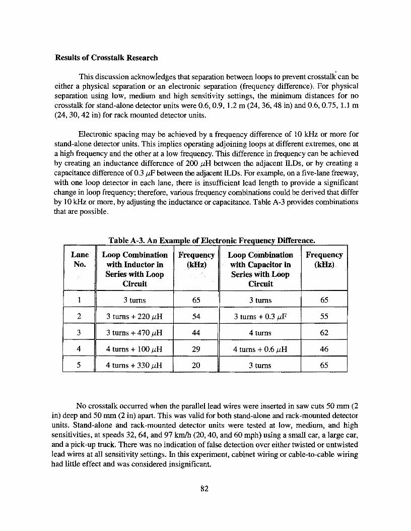
Results of Crosstalk Research

This discussion ack:now1edges that separation between loops to prevent crosstalk can be either a physical separation or an electronic separation (frequency difference). For physical separation using low, medium and high sensitivity settings, the minimum distances for no crosstalk for stand-alone detector units were 0.6, 0.9, 1.2 m (24, 36, 48 in) and 0.6, 0.75, 1.1 m (24, 30, 42 in) for rack mounted detector units.

Electronic spacing may be achieved by a frequency difference of 10 kHz or more for stand-alone detector units. This implies operating adjoining loops at different extremes, one at a high frequency and the other at a low frequency. This difference in frequency can be achieved by creating an inductance difference of 200 µH between the adjacent ILDs, or by creating a capacitance difference of 0.3 µF between the adjacent ILDs. For example, on a five-lane freeway, with one loop detector in each lane, there is insufficient lead length to provide a significant change in loop frequency; therefore, various frequency combinations could be derived that differ by 10 kHz or more, by adjusting the inductance or capacitance. Table A-3 provides combinations that are possible.

T bl A 3 A E a e - . n l fEl t . F xampeo ec romc requency n·m 1 erence.

Lane. Loop Combination Frequency Loop Combination Frequency No. with Inductor in (kHz) with Capacitor in (kHz)

Series with Loop Series with Loop Circuit Circuit

1 3 turns 65 3 turns 65

2 3 turns + 220 µH 54 3 turns + 0.3 µF 55

3 3 turns+ 470 µH 44 4turns 62

4 4 turns+ 100 µH 29 4 turns + 0.6 µH 46

5 4 turns + 330 µH 20 3 turns 65

No crosstalk occurred when the parallel lead wires were inserted in saw cuts 50 mm (2 in) deep and 50 mm (2 in) apart. This was valid for both stand-alone and rack-mounted detector units. Stand-alone and rack-mounted detector units were tested at low, medium, and high sensitivities, at speeds 32, 64, and 97 km/h (20, 40, and 60 mph) using a small car, a large car, and a pick-up truck. There was no indication of false detection over either twisted or untwisted lead wires at all sensitivity settings. In this experiment, cabinet wiring or cable-to-cable wiring had little effect and was considered insignificant.

82

Recommendations Based on Crosstalk Research

' . The spacing between lead-in wires should be 50 mm (2 in) or more. There was no

significant amount of crosstalk measured within the controller cabinet, and vehicle passage over the lead wires did not result in crosstalk, regardless of the leads being twisted or untwisted. The threshold spacing between loops for low, medium, and high sensitivity settings applicable to both stand-alone and rack-mounted detectors are 0.6, 0.9, and 1.2 m (24, 36, and 48 inches). To accommodate narrow lanes and avoid spillover detection, 1.5 m (5 ft) loops may be used without seriously affecting the electromagnetic field of the loop. Any further reduction in loop size reduces the height of the magnetic field, which reduces the probability of detecting high-profile vehicles.

THE LEAD-IN CABLE

The lead length is the length of wire from the pull box to the control cabinet. At signalized intersections, lead lengths are often less than 60 m (200 ft), whereas in the freeway environment, much longer lead lengths are often desirable. In either case, the wire is placed in waterproofed conduit approximately 45 cm (18 in) below the surface of the ground. Most manufacturers recommend grounding the lead-in cable at the cabinet (i.e., connecting the shield to the earth ground terminal) and insulating the cable in the pull box ( 12 ). This allows electrical disturbances or interference to be safely grounded without affecting the loop lead-in cable.

There has been recent research performed to establish the effects of the length of the lead-in cable on ILD performance. Woods used the controlled environment at the Texas A&M University Riverside Campus to perform this research (22 ). The test site consisted of four 1.8 m by 1.8 m (6 ft by 6 ft) ILDs, 6, 15, and 24 m (20, 50, and 80 ft) from the front edge of the first loop to the front edge of the following loop. All saw cuts in the concrete pavement were 50 mm (2 in) deep with the width of the cut varying from 6.25 mm (0.25 in) to 12.5 mm (0.5 in) depending on the type of wire used.

The first three loops consisted of six turns of # 12 THHN stranded wire, and the fourth loop consisted of six conductor (three pairs), #18 AWG, AMW style 2464, unshielded cable and were constructed with three complete turns and three individual turns. This allowed for testing of three, four, five, and six turns of wire by adding more turns, one turn at a time. The fourth loop was constructed similarly, except that the three-tum loop was connected in the pull box since the wire was six conductor unshielded. This testing also included three detector models: Detector Systems 103SS, Detector Systems 102SS, and Sarasota 515TX.

The lead cable consisted of a continuous length of two conductor #14 shielded wire. The maximum actual lead length tested was 1220 m (4000 ft). Three detector units were tested with five design vehicles which typify freeway traffic: a large car, a small car, a pickup truck, a motorcycle, and a high profile truck. Each vehicle made five passes over the loop at speeds of 32, 65, 97, and 129 km/h (20, 40, 60, and 80 mph) at low, medium, and high sensitivity settings. Each detector was tested in the presence mode of operation, where an accurate detection required

83

the detector unit to hold the call while the vehicle was within the loop. This was important, especially during the testing of the high-profile truck, since the detectors had the tendency to . detect the truck as two vehicles instead of one.

This study verified a preliminary study finding which indicated that each additional 30 m (100 ft) of lead wire added 23 microhenries of inductance. This may be achieved by connecting an inductance box in series with the system to simulate the lead lengths.

Lead Length Results

Detection of the large car, small car, and pickup truck occurred at 1220 m (4000 ft), with three, four, five, and six turns of wire for all sensitivity levels using all three detector models. Also, all five types of design vehicles can be accurately detected with a 1220 m (4000 ft) lead using medium or high sensitivity and five or six turns of wire. Any combination of fewer wire turns with low or medium sensitivity failed to accurately detect the motorcycle or high profile truck. In fact, the research indicated that detection could occur for passenger cars at even greater

distances. The type of detector unit was also a significant factor, contributing to variability in results. Considering shape, rectangular loops do not exhibit the desired performance for detection of motorcycles, and motorcycles require the shortest lead lengths (given the same detector sensitivity setting). Tables A4 and A-5 show the maximum lead lengths for accurate detection of motorcycles and trailers of high-profile trucks, respectively.

THE LOOP DETECTOR AMPLIFIER

This subject is only treated in limited detail due to two factors: 1) failure of the detector system is usually traced to the in-road detector (the loop proper) or to the splice in the pull box, and 2) the newer digital self-tuning electronic units have drastically reduced failures occurring due to the loop amplifier. There seems to be widespread agreement that failures currently being experienced in the Il.D system can be mitigated by improved installation techniques and vigilant supervision and inspection ( 12 ).

Presence or Pulse Mode

Detector units operate in either presence or pulse modes. Presence mode operation results in the detector being "on" while the loop area is occupied. Pulse mode sends a 0.1 second pulse to the controller upon detection of a vehicle. Further occupancy of the loop area by the same vehicle results in no additional action by the detector. Presence mode operation of loop detectors is preferred at isolated signals locations and for semi-actuated operation. Pulse mode is preferred for traffic counting and speed measurements. Either mode can be used in either application.

The presence of high voltage power lines under the pavement, a site with soil having high iron content, an unstable surface lift of asphaltic concrete, or undulating intersection pavement surface all have an impact on both the detector type and the controller parameter settings. The

84

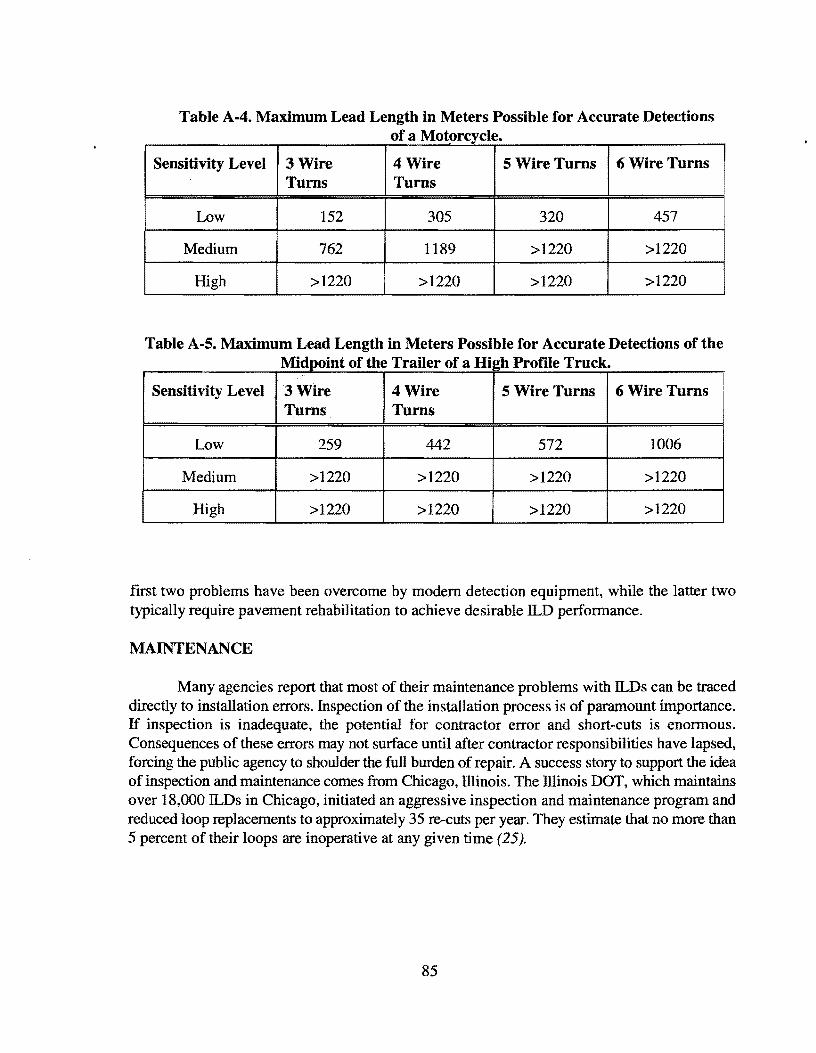
Table A-4. Maximum Lead Length in Meters Possible for Accurate Detections of a Motorcycle.

Sensitivity Level 3Wire 4Wire 5WireTurns 6 Wire Turns I Tums Tums

Low 152 305 320 457

Medium 762 1189 >1220 >1220

High >1220 >1220 >1220 >1220

Table A-5. Maximum Lead Length in Meters Possible for Accurate Detections of the Mid . t f th T ·1 f H' h Pr fll T k 1pom o e ra1ero a 1g Ole rue .

..

i

Sensitivity Level 3Wire 4Wire 5Wire Turns 6Wire Turns Tums Turns

Low 259 442 572 1006

Medium >1220 >1220 >1220 >1220

High >1220 >1220 >1220 >1220

first two problems have been overcome by modem detection equipment, while the latter two typically require pavement rehabilitation to achieve desirable ILD performance.

MAINTENANCE

Many agencies report that most of their maintenance problems with ILDs can be traced directly to installation errors. Inspection of the installation process is of paramount importance. If inspection is inadequate, the potential for contractor error and short-cuts is enormous. Consequences of these errors may not surface until after contractor responsibilities have lapsed, forcing the public agency to shoulder the full burden of repair. A success story to support the idea of inspection and maintenance comes from Chicago, Illinois. The Illinois DOT, which maintains over 18,000 ILDs in Chicago, initiated an aggressive inspection and maintenance program and reduced loop replacements to approximately 35 re-cuts per year. They estimate that no more than 5 percent of their loops are inoperative at any given time (25).

85

9.0 APPENDIX B

GRAPIDCAL RESULTS OF COLLEGE STATION FIELD TESTS

87

ACCUWAVE vs CLASSIFIER DATE= 08/21/98

50

40 E

E

a: 30

ii? E a: w E

!z E E

~ 10 E E

~ E E E E

~ 0 a: :::>

~ -10

~

~ -30

-40

E

-60

0 2 .. 6 10 12 14 16 18 24

TIME OF DAY

Figure B-1. Accuwave Hourly Percent Error vs. Classifier (8/21/98).

ACCUWAVE vs CLASSIFIER DATE= 08/22198

501 40 c

a: ~j i E w 201 E

!z E

i 10 ~ E E E

E E E E E

~ 0 "' E E E E "' "' a: B -10 ::c

~ -;!()

~ -30

-40

-so I

0 2 8 10 12 14 16 18 20

TIME OF DAY

Figure B-2. Accuwave Hourly Percent Error vs. Classifier (8/22/98).

89

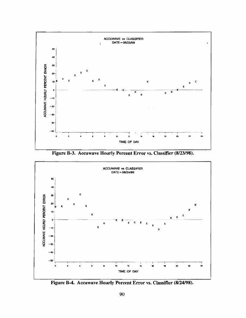
ACCUWAVE vs CLASSIFIER DATE= 08/23/98

50

40

a:: 30 0 a::

E a:: w 20 E

ffi E

E E 0 10 E E E E E a:: E w E E a.. ~ 0

~

a:: E E ::::> E E 0 -10 :c

~ ~

-20

::::>

~ -30

-40

-60 I

0 10 12 14 16 18

TIME OF DAY

Figure B-3. Accuwave Hourly Percent Error vs. Classifier (8/23/98).

ACCUWAVE vs CLASSIFIER DATE= 08/24/98

:1 j

E 5

=t a: E a: w

E I- E E E z w E 0 10

~ E E E E

~ ~ " a:: E E E E E E :::> E 0 E :c E

~

~ -30

-40

I I I

0 6 8 10 12 14 16 18

TIME OF DAY

Figure B-4. Accuwave Hourly Percent Error vs. Classifier (8/24/98).

90

a: ~ a: w

lfi ~ w a.. ~ a: ::> 0 :r:

~ ~ ~

ei a: a: w I-

ifi ~ D..

~ a: a :c w ~ ~ ~

ACCUWAVE vs CLASSIFIER . DATE= 08/25/98

501 40 .:

:t E E

E

E

10~ E

E E " E E E E

-20

-30

-40

-50 I I

0 2 10 12 14 16 18 20

TIME OF DAY

Figure B-5. Accuwave Hourly Percent Error vs. Classifier (8/25/98).

50 i

401

-30

-40 -50

2 6

ACCUWAVE vs CLASSIFlER DATE=OB/26198

E

10 12 14

TIME OF DAY

E

E

I

16

E

E

18

E

E

E e

20 22

Figure B-6. Accuwave Hourly Percent Error vs. Classifier (8/26/98).

91

24

E

ACCUWAVE vs CLASSIAER DATE=0~7/98

40

a: 30 E

a? a: w 20

ffi E

~ 10

If E

:::i 0 E a: E

:::> E E 0 -10 J: E

E E

~ E E E

-20 E E

~ E E E E

E E

5i -30

-40

-50

' I I i I

0 10 12 .. 18 18 22 24

TIME OF DAY

Figure B-7. Accuwave Hourly Percent Error vs. Classifier (8/27198).

ACCUWAVE w CLASSIFIER DATE•08128/98

50

40

i 30

20 E

~ E

10 E a: w E E E a. :::i o~·

a:

~ -10 E

~ §

-20

~ -30

-40

-50 I ' I I _,..-· ;

0 2 4 6 10 12 14 16 18 ll2 ~

TIME OF DAY

Figure B-8. Accuwave Hourly Percent Error vs. Classifier (8/28/98).

92

cc Ii? cc w

!z w 0

10

cc w Q..

~ cc => 0 :c cc

~ z

-40

-60

0

~ cc i5 -10 :c

~ -20

z -30

6

NESTOR vs CLASSIFIER DATE=08f21f98

E E E E

E

10 12 1•

TIME OF DAY

E E E

E E E E E

111 18 20

Figure B-9. Nestor Hourly Percent Error vs. Classifier (8/21/98).

E

E E

E

0 2 6 8

NESTOR vs CLASSIFIER DATE= 08/22198

E E E E

12

TIME OF DAY

E E E

E

18 22

Figure B-10. Nestor Hourly Percent Error vs. Classifier (8/22198).

93

E

E

..

a: 0

ffi

! ~ ~ a: 5 J: a:

m z

a: 0 a: a: w

!z w 0 ffi Q,.

~ a: 5 J: a: 0 I-en w z

E

E E

E E

NESTOR vs CLASSIFIER DATE= 08/23/98

E E E E E

14

TIME OF DAY

E E E

E E E E E

16 18 ..

Figure B·ll. Nestor Hourly Percent Error vs. Classifier (8/23/98).

501

:1 E

E E

:i E

E

E

-30 E

-40

-50 I

0 4 8

NESTOR vs CLASSIFIER DATE= 08/24/98

E E E E E

10 12 14

TIME OF DAY

E

E E

E

E

18 18 ..

Figure B· 12. Nestor Hourly Percent Error vs. Classifier (8/24/98).

94

E

E

a: if a: w

!z w (.) a: LU a.

~ a: :::i 0 :c a: f? ffi z

~ a: ffi

~ a:

NESTOR vs CLASSIRER DATE= 08/25/98

50

40 E E

301

:l E

E

E E E

E E E E

E

E

-30

E

-50

0 2 6 10 12 14 16 18 22

TIME OF DAY

Figure B-13. Nestor Hourly Percent Error vs. Classifier (8/25/98).

E

E

E

E E

E

NESTOR vs CLASSIAER DATE=08/26/98

E E

E E

E

5 -10 E

:c a: ~ ffj z

E E

E

0 2 4 10 12 18 20

TIME OF DAY

Figure B-14. Nestor Hourly Percent Error vs. Classifier (8/26/98).

95

E

24

E

24

~ ffi I-z ~ ffi c..

~ a:

~ a:

~ z

a: 0 a: a: w

ffi ~ c..

~ a: ::>

~

~ z

50 E

40 E

30 E

E

6 8

NESTOR vs CLASSIAER DATE=08/27/98

10 12 14

TIME OF DAY

E

E E

18

Figure B-15. Nestor Hourly Percent Error vs. Classifier (8/27/98).

NESTOR vs CLASSIAER DATE=08/28/98

so ·I E

40

E 30

20 E

E E

10

E

-40

-50 I I ' I I I I I I I

0 4 6 8 10 12 14 16 18 S) 22

TIME OF DAY

Figure B-16. Nestor Hourly Percent Error vs. Classifier (8/28/98).

96

E

I

24

a: 0 a: a: w ~ w

ffi Q..

~ a: ::::> 0 :c:

-w

~ a: Ci:

a: 0 a: ffi

I i!::i a:: :::> 0 :c ;::-w s a: Ci:

40

30

20

10

0

-10

-20

-40

-50

-10

-30

-40

-50

PIR1 (LANE 1) vs CLASSIFIER (LANE 1) DATE=08/21/98

E

E

TIME OF DAY

E E E E

Figure B-17. PIR-1 Hourly Percent Error vs. Classifier (8121/98).

0 2 4

PIR1 (LANE 1) vs CLASSIFIER (LANE 1) DATE= 08/22198

E E E E E E

8 10 12 14

TIME OF DAY

E E E

E E E

16 18 20

Figure B-18. PIR-1 Hourly Percent Error vs. Classifier (8/22/98).

97

E

E

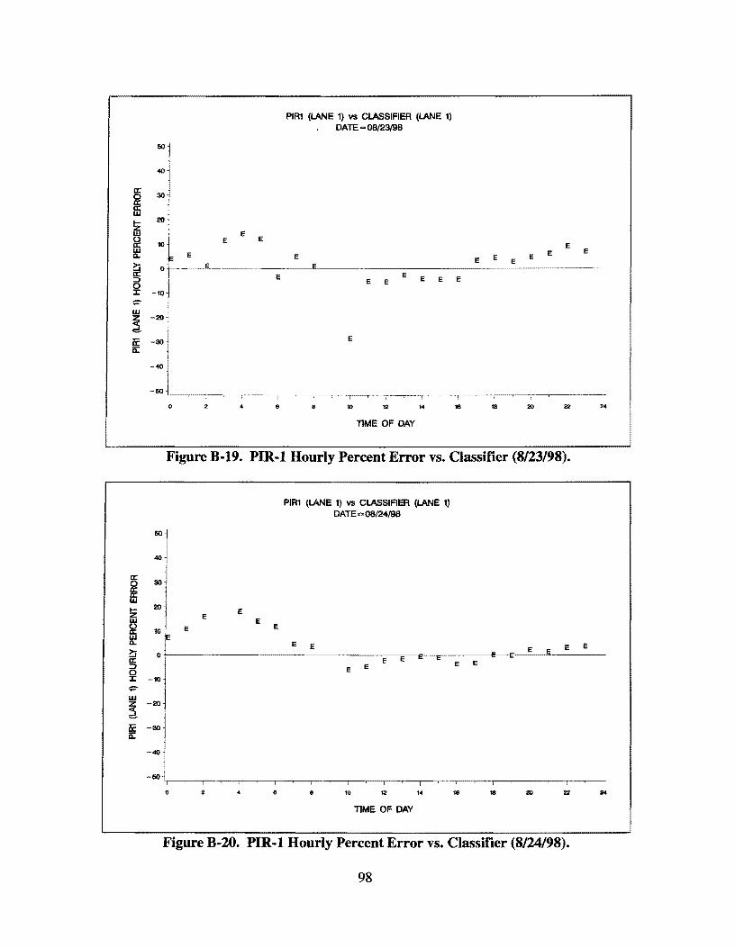
~ ffi !z w ~ ~

~ :::> 0 J: ;::-w

~ -20

lC -30 a:

-40

-ISO

40

w ~ -20

~ -30

E E E

E

E

0 2

PIR1 (LANE 1) vs CLASSIFIER (LANE 1) DATE= 08/23/98

E

E E E E E E

E

8 10 12 16

TIME OF DAY

E

E E E E

E

18 20

Figure B-19. PIR-1 Hourly Percent Error vs. Classifier (8/23/98).

0 6

PIR1 (LANE 1) vs CLASSIFIER (LANE 1) DATE=08/24/9B

8

I

10

I

12

TIME OF DAY

I

·~ I

16 ' 18

I

20

Figure B-20. PIR-1 Hourly Percent Error vs. Classifier (8/24/98).

98

E

a: fE ffi ~ w (..) a: ~ ?:::i a: :::> 0 :::c -w

~ a: a:

a: 0 a: ffi I-z

~ ~

~ :::> 0 :::c ~ w

~ a: a:

«l

30

20

50

0

-10

-20

-30

-«l

E E

E

E

E

0 6

PIR1 (LANE 1) vs CLASSIFIER (LANE 1) DATE= 08125198

8 1() 12 14

TIME OF DAY

16 18

Figure B-21. PIR-1 Hourly Percent Error vs. Classifier (8/25/98).

0 2 "

PIR1 (LANE 1) vs CLASSIFIER (LANE 1) DATE= 08126198

8 1() 14

TIME OF DAY

E E E E

16 18

Figure B-22. PIR-1 Hourly Percent Error vs. Classifier (8/26/98).

99

E

24

a: 0 a: a: w

~ ffi 0.

?:; a: :::> 0 J: ;:-w

~ er. a:

a:

i ~ w a.. ?:; a: :::> 0 J: ;:-w

~ er. a:

PIR1 (LANE 1) vs CLASSIFIER (LANE 1) DATE=08/27/98

:J

:l E

E E

E

E E

E E E E E E E E E E E E E E E

-10

-40

-ISO I I I I I I

• IO 12 14 16 18 20

TIME OF DAY

Figure B-23. PIR-1 Hourly Percent Error vs. Classifier (8/27198).

E

E E

E E E

0 •

PIR1 {LANE 1} vs CLASSIFIER (LANE 1) DATE=OB/28198

10 12 t•

TIME OF DAY

16 18 20

Figure B-24. PIR-1 Hourly Percent Error vs. Classifier (8128/98).

100

E

24

a:

i w

!z w

ffi Q..

~ a: ::> 0 J: (h

~

50

RTMS vs CLASSIFIER DATE= 08/21/98

TIME OF DAY

Figure B-25. RTMS Hourly Percent Error vs. Classifier (8/21/98).

RTMS vs CLASSIFIER DATE=00/22198

50 i

J

:J 20

10

0

-10

-20

-30

0 4 6 12 18

TIME OF DAY

Figure B-26. RTMS Hourly Percent Error vs. Classifier (8/22198).

101

a: 0 a: a: LU f-z LU 0 a: ~ ~ a: :::::> 0 ::c (J) ::!;

Ii:

a: 0 a: ffi f-z w 0 a: ~ ~ a: :::::> 0 :i: (J)

~ a:

20

10

E 0

-10

-20

0 6

RTMS vs CLASSIFIER DATE =08/23/98

10 12

TIME OF DAY

14 16 16

Figure B-27. RTMS Hourly Percent Error vs. Classifier (8/23/98).

E E

0 8

RTMS vs CLASSIFIER DATE=08/24/98

10 12

TIME OF DAY

E

14 16 18

Figure B-28. RTMS Hourly Percent Error vs. Classifier (8/24/98).

102

24

E

a: 0 a: a: LU

ffi 0 a: w ll..

~ a: ::::i 0 :I: Cl)

~

a: S? a: w

!z w (.)

~ ~ a: ::::i

2 (/)

~

50

40

30

-20

-30

-40

-50

0 2 4 8

RTMS vs CLASSIFIER DATE=00/25/98

10 12

TIME OF DAY

14 16 18 20 22

Figure B-29. RTMS Hourly Percent Error vs. Classifier (8/25/98).

RTMS vs CLASSIFIER DATE=08/26/98

501 l

:j ml~ 10

0 ~ .. E E e E E E Ii E E E E E E E E E E

-10

E

-40

-50 I I

0 2 .. 6 8 10 12 14 16 18 Ill) 22

TIME OF DAY

Figure B-30. RTMS Hourly Percent Error vs. Classifier (8/26/98).

103

ii

I

24

a: 0 a: a: w

!Z ~ a: ~ ~ a: :::> 0 :c (/)

~

a: 0 a: a: w I-z

~ ~ ~ a: a :c (/)

~

-10

-20

-30

-40

-60

E E

RTMS vs CLASSIFIER DATE= 08127198

E

E E

--------··---·---~··-~--··-~--·~-·-~·-·--··~-~-···~~-··-~····--·--1··-.----,-

0 6 10 12 14 16 18 22 24

TIME OF DAY

Figure B-31. RTMS Hourly Percent Error vs. Classifier (8/27198).

20

E

E E

-20

-30

-40

-50

0 6

RTMS vs CLASSIFIER DATE=OS/28198

10 12

TIME OF DAY

14 16 16

Figure B-32. RTMS Hourly Percent Error vs. Classifier (8/28/98).

104

er: 0 E er: er: w E

!Z 10 ~ er:

E E

E E ~ 0

~ -10 :::>

2 Q -20 z ~

-30

-40

0

TIME OF DAY

Figure B-34. SmartSonic vs. Classifier (8/22/98).

105

50

a: 0 a: ffi

~ E E

a. ~ a: :::> -10 0 :c Q -2(1

~ -30

-40

-50

0

50i

j

40 l E

a: 301

0

:i E

a: ffi !z ~ w a. ~ a: 8 :c (.) -20

§ -30

0

E E

E

E E E

SONIC vs CLASSIFIER DATE= 08/23/98

10 12

TIME OF DAY

E

14 18

Figure B-35. SmartSonic vs. Classifier (8/23/98).

SONIC vs CLASSIFIER DATE= 08/24/98

E

E

E E

E

E

.. 8 10 12 16 16

TIME OF DAY

Figure B-36. SmartSonic vs. Classifier (8/24/98).

106

E

E

E

E E

E

SONIC vs CLASSIFIER DATE=OS/25/98

!M) l E

401 E

30 ~ E

a: 0 E a: E a: w E

!z 10 E

~ E E E E a: E w

0 a.. ~ E a: :::> -10 0 ::c 0 z 0 en

-30

-40

-50 ~-----,-.-.--1-r ·---,·

0 2 6 10 12 14 16 16 22 24

TIME OF DAY

Figure B-37. SmartSonic vs. Classifier (8/25/98).

SONIC vs CLASSIFIER DATE<=08/26/98

50 E

E E

a: E 0 a: E a: w

i E

E E E E

a.. ~

E

a: -10 :::>

0 ::c 5.2 -20

~ -30

-40

-50

0 " 4 10 12 14 18

TIME OF DAY

Figure B-38. SmartSonic vs. Classifier (8/26/98).

107

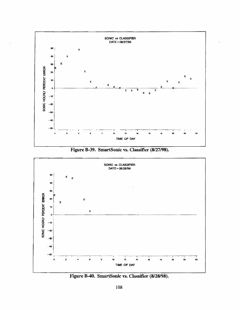
50i

401 j

~~ E a: ff ffi

20 ~

!z ~ a: w 0..

::i cc ::i -10

~ !'::? -20 z &$

-40

-50 :

a: if a: w E

!z

~ ~ a: 8 J: !'.,,;! z 0 Cl)

-~

-40

-60

0

E

SONIC vs CLASSIFIER DATE=08/27/98

E

E

E E

E ~ "' - E

E E E E E E

I

4 3 10 12 14 16 16

TIME OF DAY

Figure B-39. SmartSonic vs. Classifier (8127198).

SONIC vs CLASSIFIER DATE= 08/28198

E E

E

E

2 6 6 10 12 16

TIME OF DAY

Figure B-40. SmartSonic vs. Classifier (8/28198).

108

E E

E

~

I I

22 24

-g

300

250

200

I.are Ore Counts 812()..8121 --------·~ + Cl..A$_Ll 1111 s::NC_Ll RTMS_Ll ' NESI'_Ll '.:*: PIR-l_Ll

~ = ~o ---<::> u

100

50

0 ·----; ---+----·+-----+ ----+--- -+-----+---

10:30 AM 12:00PM 1:30PM 3:00PM 4:30PM 6:00PM 7:30PM 9:00PM 10:30PM 12:00AM 1:30AM 3:00AM 4:30AM 6:00AM 7:30

'IlnE ---------------------------- ·--· ·--· ----~ ----------------

Figure 8-41. Raw Data Plot Lane One (8/20-8/21).

250

200

l3 g -- u 100 0

50

time Two C.Ounts 8/20-8121

e SJNIC_L2 RTMS_L2 " NF.ST _L2 -~~-~~

R" Pl

12:00PM 1:30PM 3:00PM 4:30PM 6:00PM 7:30PM 9:00PM 10:30PM 12:00AM 1:30AM 3:00AM 4:30AM 6:00AM 7:30AM

'lb:JE

Figure B-42. Raw Data Plot Lane Two (8/20-8/21).

-...... -

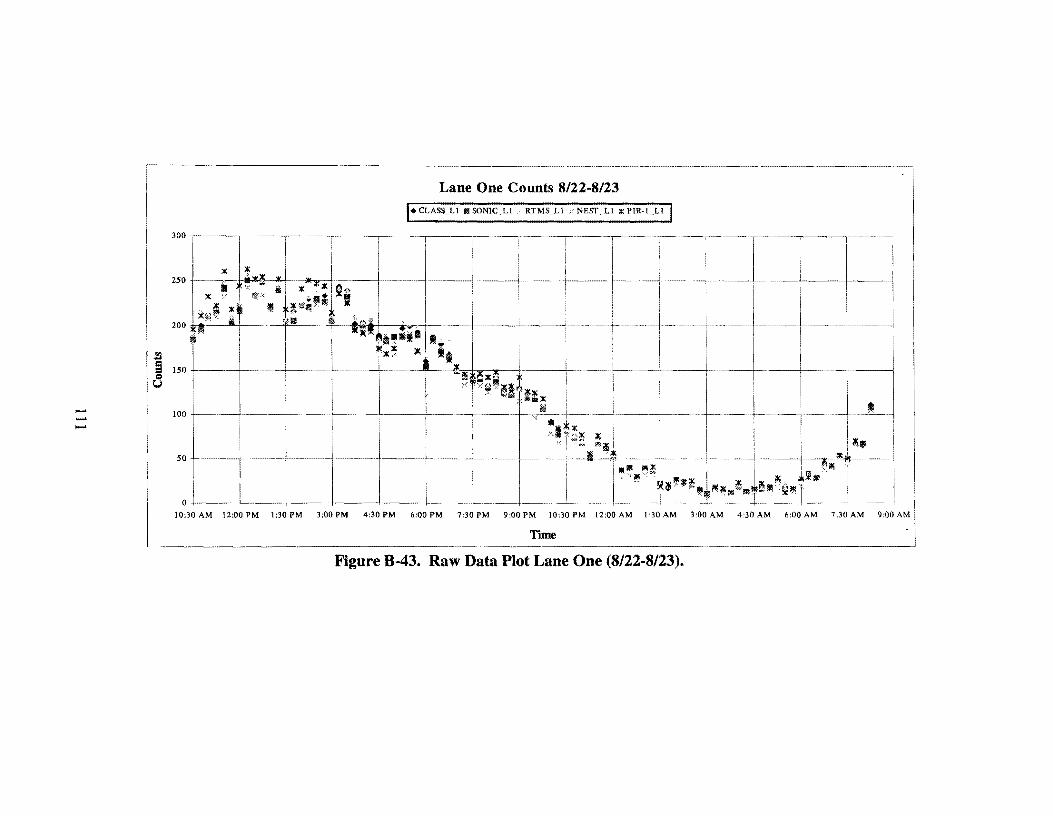
Lane One Counts 8/22-8/23

[+cLASS_Ll 1111soN1c_u RTMS_Ll ,cNEST_L1 :i:PIR-1_L! I 300~---

250

200 J;A ""I 'f- · 4-·ll!lihll I 't"'-c:-+-------·--1-------+----i--

:l 5 ISO

100 ·I----··---+---+----

so~- --+

0 +--- !----. ----

10:30 AM 12:00 PM 1:30 PM 3:00 PM 4:30 PM 6:00 PM 7:30 PM 9:00 PM 10:30 PM 12:00 AM 1:30 AM 3:00 AM 4:30 AM 6:00 AM 7:30 AM 9:00 AM

Time

Figure B-43. Raw Data Plot Lane One (8/22-8/23).

Lane Two Counts 8/22-8/23

RTMS_L2 :'" NEST_L2 ------~~~~~~~---

160

140

120

100

I 80

u - I 60 __ ____j_ __ -N Ill

40 ll'---

20

0 10:30 AM 12:00 PM 1:30 PM 3:00 PM 4:30 PM 6:00 PM 7:30 PM 9:00 PM 10:30 PM 12:00 AM 1:30 AM 3:00 AM 4:30 AM 6:00 AM 7:30 AM 9:00 AM

Time

Figure B-44. Raw Data Plot Lane Two (8/22-8/23).

,_. ,_. w

---- -----

lane One Counts 8/23-8124 -------·~----

• <LAS'>_Ll 111 SJNIC_Ll RI'MS_Ll NESI'_Ll ~ PIR-l_Ll

250

200

150 );

100 +ll0-----1------

50 - ~+- --+

0

9:30 AM 11:00 AM 12:30 PM 2:00 PM 3:30 PM 5:00 PM 6:30 PM 8:00 PM 9:30 PM 11 :00 PM 12:30 AM 2:00 AM 3:30 AM 5:00 AM 6:30 AM 8:00 AM 9:30 AM

1inE ------ ----

Figure B-45. Raw Data Plot Lane One (8/23-8/24).

200

180

160

140

:i 120

§ 100 0 u 80

60

40 -I - 20 .J:>..

0

9:30AM 11:00 AM

Lane Two C.ounts 8123-8124

[~a.A'iS_L2 llllS()l'IIC_L2 _ -~

12:30PM 2:00PM: 3:30PM 5:00PM 6:30PM 8:00PM 9:30PM ll:OOJ'f\i 12:30 2:00AM 3:30AM 5:00AM 6:30AM 8:00AM 9:30AM AM

Time

Figure B-46. Raw Data Plot Lane Two (8/23-8/24).

--Vl

1.a:EOeilim W243'15 ~~-u ISNCJ.1 RIMS_U xN:fil~u~H.R-=i~u]

:r-lu-u l-~---1-----1 l.i .

~ani ,,II~ § 15'.) 0 u100

5'.) +----- --+ -

9.lJAM llillAM LrnIM 2:00IM 3:lJIM 5illIM 6:lJIM 8.illIM 9-.lJIM llillIM 12:lJAM 2illAM 3:lJAM 5illAM 6:lJAM 8.illAM 9.lJAM

1hte

Figure B-47. Raw Data Plot Lane One (8/24-8/25).

.......

....... 0\

250

200

ll 150

a Q u 100

50

0

I

Lare T\"IDCCl.ns 8'24-8'25 l+~_l2 II __ SONIC_l2 RTMS_l2 :l'.NEST_l2 ------

... ';;~ j.\

~'

9::IDAM 11:00 12::ID 2:00PM 3::IDPM 5:00PM 6::IDPM S:OOPM 9::IDPM 11:00 12::ID 2:00AM 3::IDAM 5:00AM 6::IDAM S:OOAM 9::IDAM AM PM PM AM

'I'i:nE

Figure B-48. Raw Data Plot Lane Two (8/24-8/25).

,_. ,_. --...}

l.aJE OtE Comts 8126-M7 I• ~-Ll 11111 IDNIC_Ll RTMS_Ll NE.~ _Ll :« [____ -~~~~~~~-~~---~·---'

300

I

250 i •• I nnu - - --1----+-· ··-·- +-- ·--+ ·--· +-----4·--·

~ .* ,: ••:t::~' x. m~ •• ·.

200 +----- . .. ···-··· -- ·-· fl'l I · x •Iii '- .····· ~ I 1_~ ~ 1xx ~

::t'~ "' _____ _j

I I I

100 ~ I ... +~~- f---·~ I I~' I

so -;-~., .. Ml. •!~··· :. --t r ~' 1111111 l111'f'l1! : ,; ' 0 --- .. .,. ... ··--+-----+

l:OOPM 2:30PM 4:00PM 5:30PM 7:00PM 8:30PM lO:OOPM 11:30PM l:OOAM 2:30AM 4:00AM 5:30AM 7:00AM 8:30AM

ThrE

Figure B-49. Raw Data Plot Lane One (8/26-8/27).

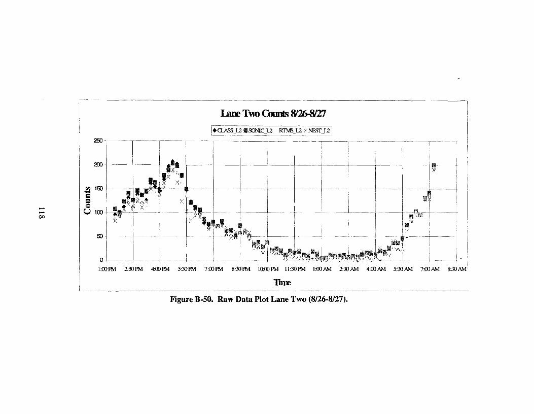
l.aIE '!\lo Counts 8f1b.WZ7

F~-12111SONic_12 RTMS_u-;;;Nifil_u I 25)

a:n ... ,

--00

!°l 150 . · II, d I I ,Ill = : 1111.y x,.,~ Q j II t· ·.} X u 100 i H~I ! - ---- ---- +-c;;G•---t---·

j li' I

50 i -------· -1 -oLL ----- ~-- -'£·\.~_::.·_,_(~~,~

l:OOP!'vi 2:30Pl'vi 4:00Pl'vi 5:30Pl'vi 7:00Pl'vi 8:30Pl'vi lO:OOP!'vi 11:30Pl'vi l:OOAM 2:30AM 4:00AM 5:30AM 7:00AM 8:30AM

ThtE

Figure B-50. Raw Data Plot Lane Two (8/26-8/27).

,....... ,....... \0

!are fu Outs 8/Z7-NJS 1·-UA~.J_..111 &NC_Ll RTMS_uN!fil_11.~f>rR-u11

300

250 +--··--!

:mt• I l_~Ll:r~U ·.. I -=+- -+-· ...j-n l~~BI•- ftMwl ii~ ! X~I .. :s § 150 +---·iilii..~"-1 ·~~''--" e u

100

50

0

7:30 AM 9:00 AM 10-.30 AM 1200 P.M 1:30 P.M 3:00 PM 4:30 PM 6:00 PM 7:30 PM

'Due

Figure B-51. Raw Data Plot Lane One (8/27-8/28).

l

....... N 0

!

Lane Two Counts 8/27 -8/28

)<NEST_L2

250 .,...---~--~-

200 .+---------+------- --4-----------+-~-- --+------+----

150 +--------------+----- -------t - - ------! ~ - ----+---~----+--

100 ~--------------

50 +--- ---------------1-----1---+----

0 7:30 AM 9:00 AM 10:30 12:00 PM 1:30 PM 3:00 PM 4:30 PM 6:00 PM 7:30 PM 9:00 PM 10:30 PM 12:00 1:30 AM 3:00 AM 4:30 AM 6:00 AM 7:30 AM

AM Time

AM

Figure B-52. Raw Data Plot Lane Two (8/27-8/28).

10.0 APPENDIX C

GRAPIDCAL RESULTS OF HOUSTON FIELD TESTS

121

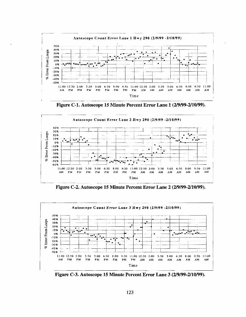
"' c.. 8

....:i

~ µ., .... 6 Ul

lf

"' g ....:i

~ .... 6

Ul

lf

Autoscope Count Error Lane 1 Hwy 290 (219199 -2110/99)

50% 40%

30% 20% 10%

0% -10% -20% -30%

i : • I • •' . :

: . I . . ... • • • • • & I& ••

. . I+ • • . •-; • •• • . :+

-. ~. •• . . • -·· . . I• .... ~ . . . . •• i •• '• -

I i I I ··-·

-40% -50%

i ·--r----~-

I I

11:00 12:30 2:00 3:30 5:00 6:30 8:00 9:30 11:00 12:30 2:00 3:30 5:00 6:30 8:00 9:30 11:00 AM PM PM PM PM PM PM PM PM AM AM AM AM AM AM AM AM

Time

Figure C-1. Autoscope 15 Minute Percent Error Lane 1 (2/9/99-2/10/99).

Autoscope Count Error Lane 2 Hwy 290 (219199 -2/10/99)

40% 30% 20% 10%

0% -10% -20% -30% -40% -50% -60%

I : I ,_

·1 I l I I : . :---_J

I I I I I : -. I•+ - . . • • :• • •• t ·• .T • .• : . . ...

-1 1· ' I i

--, __ , I • .

I I . ~' _,_I-··- ---

i . __. • . . I • • I I •• I I - .l ... , I . ---.-.. I • •

..... I .......... ~·-·· . t •

11:00 12:30 2:00 3:30 5:00 6:30 8:00 9:30 11:00 12:30 2:00 3:30 5:00 6:30 8:00 9:30 11:00 AM PM PM PM PM PM PM PM PM AM AM AM AM AM AM AM AM

Time

Figure C-2. Autoscope 15 Minute Percent Error Lane 2 (2/9/99-2/10/99).

Autoscope Count Error Lane 3 Hwy 290 (219199 -2/10/99)

50% : II~--,,,,,, I,,

40% +---~1----i~-r --+---r---+----+----+----t--i.---+-----+---+----+-- -1-------1

30% +---~1 ----1--+---~--~,,,,, .. --+----+--.+---hr•'--1--+---+---+----+---"-----t

~~: & • I • • • ................ 0% • ··i:'~' ...... ··•. . .. ..

-10% + • • • l • •·~+ r-~ •• -+-.-+---+--- i------+---+---+-------+

~~~: +--+--l--,-i----1~•--r---+o....--•-71 + -

-40% I -50% ~-~1--1-----•--~--~--+----~-~-~--+--~'-··········-'-----~- --+----~----~

11:00 12:30 2:00 3:30 5:00 6:30 8:00 9:30 11:00 12:30 2:00 3:30 5:00 6:30 8:00 9:30 11:00 PM PM PM PM AM AM AM AM AM AM AM AM

Time

Figure C-3. Autoscope 15 Minute Percent Error Lane 3 (2/9/99-2/10/99).

123

"' J El s ....

~ ~

"' c.. g

.....l El .g .... g

f.ll ~

Nestor Count Error Lane 1 Hwy 290 (2/9/99 -2110/99)

60%

50%

40%

30%

20%

10%

0%

•I -

I i. I +· ... i ... ..... • f"'

• -. .. ... .. - •• : .... ' ... • , .. ·. i • • .!• - i- -... ·· l.• -· i••· • •• •• • - • • • .... ••• .. - • . -··--,- --~-·- • ... ... ..

-10%

-20%

-30%

. I I I ;

·--

11:00 12:30 2:00 3:30 5:00 6:30 8:00 9:30 11:00 12:30 2:00 3:30 5:00 6:30 8:00 9:30 11:00 AM PM PM PM PM PM PM PM PM AM AM AM AM AM AM AM AM

Time

Figure C-4. Nestor 15 Minute Percent Error Lane 1 (2/9/99-2/10/99).

-----------------····--1

Nestor Count Error Lane 2 Hwy 290 (2/9/99 -2110/99)

I : I I i I ' I i

I :

50%

40%

30%

i I . •i• ! ~· • -• .. ~ .. ...... T .

• . . • • ..... _ ... . .... ....... t ..... . .... •• I . ........... ~· . .·r • ·- • i I . I i I i ;

-30%

20%

10%

0%

-10%

-20%

11:00 12:30 2:00 3:30 5:00 6:30 8:00 9:30 11:00 12:30 2:00 3:30 5:00 6:30 8:00 9:30 11:00 AM PM PM PM PM PM PM PM PM AM AM AM AM AM AM AM AM

Time

Figure C-5. Nestor 15 Minute Percent Error Lane 2 (2/9/99-2/10/99).

Nestor Count Error Lane 3 Hwy 290 (2/9/99 -2/10/99)

I I • • I

I .. • • ! ... i 10% +------+---+--f----t----+----z--+-....... -----+---+---+---+---+--1----~

0% ' •r~··-+~.,.~-+---+---+-4>--+--l-•-+---!l--~--+---10% I ......... I • I .. ·..,...;:. • • I . • • • • l

• .1 ..... • ...... • ,. ... ..... ~--·-+-.---+-+--.-+-.--+-__,I,___,+---···+. • • • -20% ... • • ... •• •• ' ' • ... • •

I '•

i

20%

I • T• I ...... ! ... • •

~~:~:_,_• __ ,_I I • I :

11:00 12:30 2:00 3:30 5:00 6:30 8:00 9:30 II :00 12:30 AM PM PM PM PM PM PM PM PM AM

Time

2:00 AM

3:30 AM

5:00 6:30 8:00 9:30 AM AM AM AM

Figure C-6. Nestor 15 Minute Percent Error Lane 3 (2/9/99-2/10/99).

124

11:00 AM

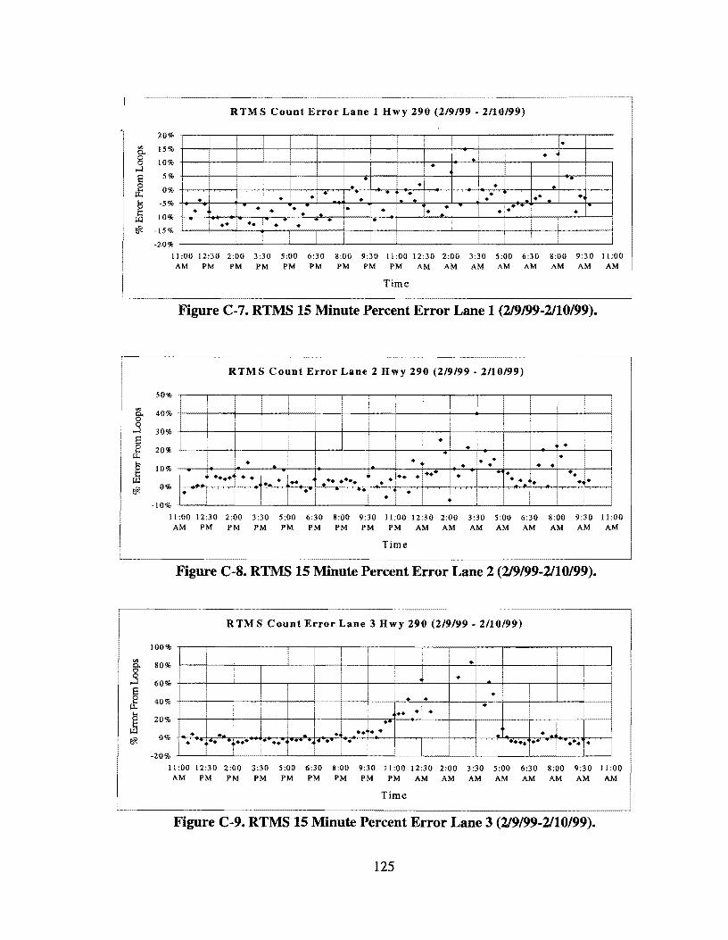
.,, p..

8 .....l e 0 u: !:l Jj ~

"' p.. 0 0

.....l s 8

I.I.. ... g U..l !ffe

"' ! e £ ....

.E !§i

Count Error Lane 1 Hwy 290 (2/9/99 • 2/10/99)

20%

15%

10%

5%

0%

-5%

-10%

-15%

-20%

I I ! • I ! I • 1 •

I • I I • I •I

. • . .

I • r·····; . ... ·: I

.'T ••• .,. •• • T ~ -~ . • • • • ... .. .. • •

• :• - • T· • .: . . - . • ; • . - • - •

•• 1· •: T • • I I l •• • • i I I I I

11:00 12:30 2:00 3:30 5:00 6:30 8:00 9:30 11:00 12:30 2:00 3:30 5:00 6:30 8:00 9:30 11:00 AM PM PM PM PM PM PM PM PM AM AM AM AM AM AM AM AM

Time

Figure C-7. RTMS 15 Minute Percent Error Lane 1 (219/99-2/10/99).

R TM S Count Error Lane 2 Hwy 290 {2/9/99 • 2/10/99)

50%

40%

30%

20%

10%

0%

! I I I

I ! I I I i I

I I

i I I I

I I I I ! • I I I I i • •

I ! . ~ • 1 •• • • - I • ' . • •

i . ••••• 'i •• l :1 .!•• . 1··· ! • 1· •• ... ·· ..... • • • • ·- - • I ~r·.._, . •'

I ·1 I .. - ... ,--- .. •

I + I ! • -10%

11:00 12:30 2:00 3:30 5:00 6:30 8:00 9:30 11:00 12:30 2:00 3:30 5:00 6:30 8:00 9:30 11:00 AM PM PM PM PM PM PM PM PM AM AM AM AM AM AM AM AM

Time

Figure C-8. RTMS 15 Minute Percent Error Lane 2 {2/9/99-2/10/99).

RTM S Count Error Lane 3 Hwy 290 (219199 • 2/10/99)

100%

80% !

60%

I I .i I :

! . • I

• 40%

20%

. . I I •

; . .. • • , I •·

0% . . i ... • ~ .... ·~ . -. ~·· ... .,.. ! ,,,. •• -1-... • .. • •""' ..... ! ·--r+~~i-.-r~+,,-m~~,..-- ••+. ..... I .•~· ~

-20% -'-~-'-~~~-'-~--'-~--J;__~.1--~~~--'--~-L..~-L~--'-~~~~.I--~~~-'-~-'

11:00 12:30 2:00 3:30 5:00 6:30 8:00 9:30 11:00 12:30 2:00 3:30 5:00 6:30 8:00 9:30 11:00 AM PM PM PM PM PM PM PM PM AM AM AM AM AM AM AM AM

Time

Figure C-9. RTMS 15 Minute Percent Error Lane 3 {219199-2/10/99).

125

"' g ...J E 0 ....

i:.. ....

~ ~

Autoscope Count Error Lane 1 Hwy 290 (2/10/99 -2111/99)

60%

50%

40%

30%

20%

10%

0%

-10%

-20%

-30%

i i

. i I • : I . !

I • .. . i •• l • i

! ! ••• •• • • • - -.1~!. ! •••

•.+ . •• + •• . • • ·- •• I+ • ,. ··.!. ·--... . . • --.•1 • . . _. ••

-····

I -------

I I i

11:30 1:00 2:30 4:00 5:30 7:00 8:30 10:00 11:30 1:00 2:30 4:00 5:30 7:00 8:30 10:00 AM PM PM PM PM PM PM PM PM AM AM AM AM AM AM AM

Time ~----···· - -----~ ----~~~-----

Figure C-10. Autoscope 15 Minute Percent Error Lane 1 {2/10/99-2/11/99).

Autoscope Count Error Lane 2 Hwy 290 (2/10/99 -2/11/99)

80%

"' 60% s:i.. 0 0 40%

...J E 20% 0

0% .... i:.. .... -20% 0

Jj -40%

~ -60% .... ~ ..... .

• • -80%

11 :30 l :00 2:30 4:00 5:30 7:00 8:30 10:00 11:30 1:00 2:30 4:00 5:30 7:00 8:30 10:00 AM PM PM PM PM PM PM PM PM AM AM AM AM AM AM AM

Time

Figure C-11. Autoscope 15 Minute Percent Error Lane 2 {2/10/99-2/11/99).

Autoscope Count Error Lane 3 Hwy 290 (2/10/99 -2111/99)

200%

160%

"' g. 120% .3

~ 80%

40% !;i

-l-.... ~ 0%

~ -40%

-80%

11:30 1:00 2:30 4:00 5:30 7:00 8:30 10:00 11:30 1:00 2:30 4:00 5:30 7:00 8:30 10:00 AM PM PM PM PM PM PM PM PM AM AM AM AM

Time

Figure C-12. Autoscope 15 Minute Percent Error Lane 3 {2/10/99-2/11/99).

126

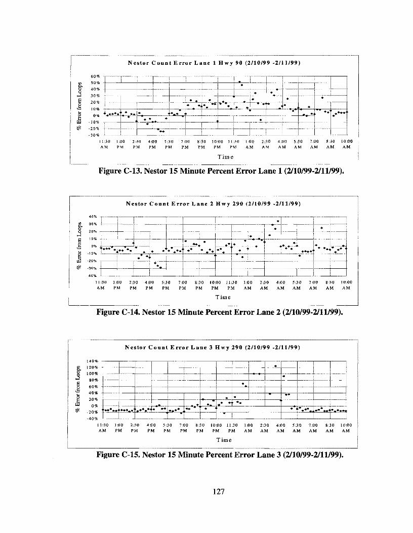
~ 0

3 8 .g

~ ~

"' 0. 0 0

...-l E 0

cl::

~ ~

i!i. 0

.3 E 0

cl:: ....

~ ~

Nestor Count Error Lane 1 Hwy 90 (2/10/99 -2/11/99)

60%

50%

40%

30%

20%

10%

0%

-10%

-20%

-30%

! - I I I I • !

~-·----

;

i • • . - • • • • • ·~ ·. -.. -. .1

... ,.... • I • - • .. .... • .l. ..... ··~ •••• ..... ~ • .... • ·-· -• • • • - I • • --r-·~

I ; -. I I

11:30 1:00 2:30 4:00 5:30 7:00 8:30 10:00 11:30 1:00 2:30 4:00 5:30 7:00 8:30 10:00 AM PM PM PM PM PM PM PM PM AM AM AM AM AM AM AM

Time

Figure C-13. Nestor 15 Minute Percent Error Lane 1 (2/10/99-2/11/99).

Nestor Count Error Lane 2 Hwy 290 (2/10/99 -2/11/99)

40%

30%

20%

10%

0%

-10%

-20%

-30%

-40%

11 :30 l :00 2:30 4:00 5 :30 7 :00 8:30 10:00 11:30 PM PM AM PM PM PM PM PM PM

Time

Figure C-14. Nestor 15 Minute Percent Error Lane 2 (2/10/99-2/11/99).

Nestor Count Error Lane 3 Hwy 290 (2/10/99 -2111/99)

140%

120%

100%

80%

60%

40%

20%

0%

-20%

I I ! • I

I I I I

t~ I •

i ! I • --····-· I ----

I I I !• .. ••

...... • I I I

.. ., .. - • ·- :.• ... -· --·¥··r .. • t • ·~; . ...._ ••• ..J. • .... l -:

.....•. I

-······

-40%

11:30 1:00 2:30 4:00 5:30 7:00 8:30 10:00 11:30 1:00 2:30 4:00 5:30 7:00 8:30 10:00 AM PM PM PM PM PM PM PM PM AM AM AM AM AM AM AM

Time

Figure C-15. Nestor 15 Minute Percent Error Lane 3 {2/10/99-2/11/99).

127

"' 0. 0 0

....:i e £ ... s If:

"' 0. 0 j e £ ... s If:

RTM S Count Error Lane 1 Hwy 290 (2110/99 - 2111/99)

30% 25%

I . I I i

20% 15%

10% 5%

I • I : - :

I I : • I I ' I .,1 .. j •, - 1•• . . I '

·-~ T .. T .... f 0%

-5% I • ..... . I :• - ·- ... ~ I • •• ·- • • -10%

15%

-20%

• ··1·. t+·· •• • •J_ - .-. . ~

• I . .. - • • '"'1'

I I ~ I I 11:30 1:00 2:30 4:00 5:30 7:00 8:30 10:00 11:30 1:00 2:30 4:00 5:30 7:00 8:30 10:00

AM PM PM PM PM PM PM PM PM AM AM AM AM AM AM AM

Time

Figure C-16. RTMS 15 Minute Percent Error Lane 1 (2/10/99-2/11/99).

RTMS Count Error Lane 2 Hwy 290 (2110/99 • 2111199)

35% . ! 30%

25%

20%

15%

10%

5%

0%

-5%

-I 0%

. - -+ I I :

I - I - I I • I ...

_T • - • ·- . += . • • . •. :+ ·-

• . ,. ·- :•• .... ~ ... • . . ·.i •• • I . .+ . .--. . ' •• • .

• • . . t ...• T

I • . . . I i . T I

11:30 1:00 2:30 4:00 5:30 7:00 8:30 10:00 11:30 1:00 2:30 4:00 5:30 7:00 8:30 1 AM PM PM PM PM PM PM PM PM AM AM AM AM AM AM

Time

Figure C-17. RTMS 15 Minute Percent Error Lane 2 (2110/99-2/11/99).

R TM S Count Error Lane 3 Hwy 290 (2/10/99 - 2/11/99)

60%

• 40% •

• • 20%

1 •••

.. • • • • ·hi ~.-r-<0+,--.~.--t=~._,.+~,._;~~-t-r-~r-i-~-rci.~ =.-r,,_-,<-=<;-.~.~ • .,-,--t

• • • • • •• • • ••

• • 0%

I I

;

11:30 1:00 2:30 4:00 5:30 7:00 8:30 10:00 11:30 1:00 2:30 4:00 5:30 7:00 8:30 10:00 AM PM PM PM PM PM PM PM PM AM AM AM AM AM AM AM

T

Figure C-18. RTMS 15 Minute Percent Error Lane 3 (2/10/99-2/11/99).

128

50%

40%

30%

20%

10%

0%

10%

Autoscope Count Error Lane 1 Hwy 290 (2111199 -2113/99)

:! < 1'l =

~ l ~ ~ ~ g 8 g ,..... N ~ Vi

:! :! .. .. 8 g

"' ;.;

::! l .. 8 1'l ~ =

:! < ~ "

:! :! ::! ~ ::! ::! < < < < .. g ?. ~ 8 : § .;; ~ s

Time

::! ::i! l ::! :! l ::! ::! ::!! ::! ::! .. .. .. .. .. < < < < g 8 ~ 8 g 8 1'l 3 g 8 g N .;,; "' 00 :2 = ;; .;,; .;;

::i! ::i! ::! < < <

~ g ~ 00

~····---~~···---·---····---····---·--------- --- -----

Figure C-19. Autoscope 15 Minute Percent Error Lane 1 (2/11/99-2/13/99).

Autoscope Count Error Lane 2 Hwy 290 (2/11/99 -2/13/99)

50%

"' 40% g 30% ....< e 20%

&; 10%

.... 0% g 10% r.a

~ -20%

-30% :! ::i! ::! ::! ::! ::! ::! ~ ::! ::i! ::! ::i! < .. .. .. .. .. .. .. < < < 1'l § g ~ ~ ?. 0 8 ~ ?. 0 ?. = ;; ;.; ~ - "' ,,

::i! ::! ::i! ::! ::i! ::i! l l ::! ::! l l ::! < < < < < .. .. .. .. :ii 8 g 8 TI ~ g ?. g ~

"' 8 ~

~ "' " s Oi " .;; s ::! ::!! ~ ::! ::i! ::! :! ::! < < < < < < < ~ g ~

0 8 ~ 8 ~ - ;; .;; "' " §

Time

Figure C-20. Autoscope 15 Minute Percent Error Lane 2 (2111/99-2/13/99).

Autoscope Count Error Lane 3 Hwy 290 (2/11/99 -2/13/99)

50%

! 40%

30%

~ 20%

.t 10%

~ 0%

-10%

I;§< -20%

-30%

: I I ····1 I I i I i I I ! I I •• I

_.J : I I • ... ! ·~ .. I _J

I i ·' I I • .. r • "'- •J."t. I i I ..... - __, ,.. ~ .... ·-'.o.• ...

.-r~~ .,;.. ~

I - I . , • ... I " ~" ~i. : I I • i•

I . ~ .! ... ,. I I ~ • ~ i - .. ~ •..

... • 1• ... 1• ... I I ...,~.-.~_! I

~ ::i! t t t t t t t ~ ~ ~ ~ ~ ~ ~ ~ t t t t t ::! t t ~ ~ ~ ~ ~ ~ ~ ~ .. .. ~ ?. ;;\ ~ :;;, ?. :;\ 8 :;;, €; ;;\ ?. ;;; ~ :;;, 8 "' § "' 8 "' ~ ;;\

~ ;;\ ?. :;; ?. ~ ~ :;< ?. ~ = - "< "' ~

., ~ ;: M "' ... "' "° ~ =

"< ~ v; "° ::: "° ~ ;:

Time

Figure C-21. Autoscope 15 Minute Percent Error Lane 3 (2111/99-2113/99).

129

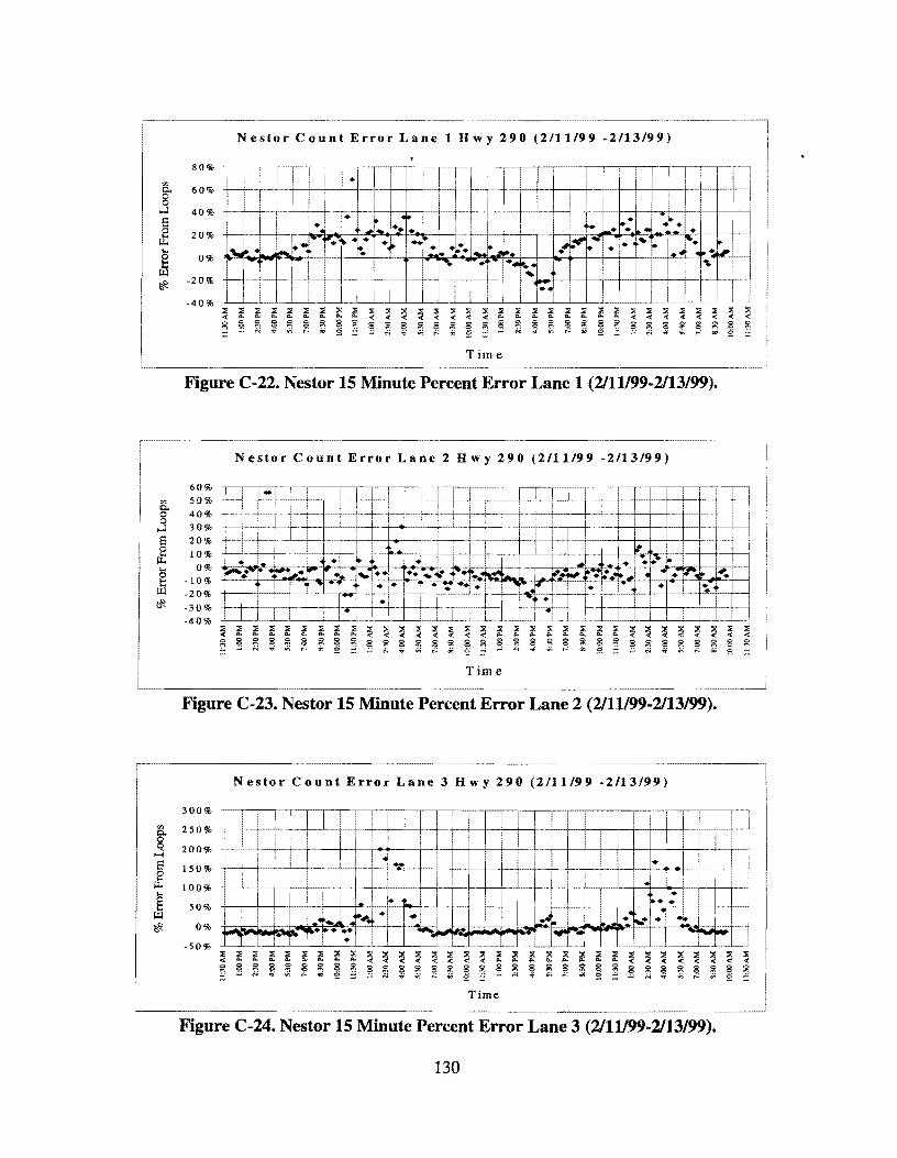
Nestor Count Error Lane 1 Hwy 290 (2/11/99 -2/13/99)

0%

-20%

-40% ;:;: ::;; t ;:;: ::;; ;:;: ::;; ;:;: ::;; < .. .. .. .. .. .. .. ~ ~ :;;; 8 g 8 g

~ ~ "' "' v; "' .;;

;:;: ;:;: ::;; ::;; ::; ::; ::;; ;:;: ::; ;:;: ::; ;:;: ;:;: ;:;: ::;; ::; ::;; ::; ::;; ::; < < < < .., .. .. .. .. .. .. .. < < < < .., .., < < g 8 0 8 s ~ g

~ 0 8 ;;; 0

8 :>; 8 li: 8 g 8 : .., .., v; ... " § "' v; "' .;; :::: 'f v; "' .. §

Time

Figure C-22. Nestor 15 Minute Percent Error Lane 1 (2/11/99-2/13/99).

Nestor Count Error Lane 2 Hwy 290 (2/11/99 -2/13/99)

60%

"' 50% Q.,

40% 0

3 30%

s 20%

£ 10%

... 0% 0

-10% I:: Ill -20% ~ -30%

-40%

! i I ' I ! Tl I I -::ir-, •

I I I

I I I i I !

l i .... i I II' I ' -- I ·~. ! ' . .... loo . • • ' ...I - ._.1 .• I

-+- ..-.~-~•;,,r • -·r ._"'_l#_'.'t- •• ·~1·., •• ... -,t . .... ~. llL~~~ ,:: .• ... • '"'!."' • ~

! I .. -! • 1· , •: •• • "' • I

. •1 ~ -- • i '"' • I I I • I !

-· " I ! I

::; ::; l ::; ;:;: ::; ::; t ;:;: ;:;: ;:;: ::; ::; ;:;: ;:;: ;:;: ;:;: ;:;: ;:;: ::;; ;:;: ;:;: t l t ;:;: ;:;: ;:;: ::; ;:;: ;:;: < .. .. .. .. .. .. < < < < < .., < .., .. .. .. .. .. < .., .., .., .., < ~ 8 Pi 8 Q 8 g 8 ii\ g g 8 Pi 8 g g ~ ~ :;\ 8 :>; g ;;;

~ :;\ ~ g ~ ~ g g - "' 'f v; ... ;; s ::: - N .. v; ... .;; ~ N 'f ~ "' " ::: N ... ,;;

Time

Figure C-23. Nestor 15 Minute Percent Error Lane 2 (2/11/99-2/13/99).

Nestor Count Error Lane 3 Hwy 290 (2/11/99 ·211

300%

"' 250% Q.,

3 200%

s 150%

£ 100%

'"' § 50% Ill .. ~ 0%

-50% ;:;: ::; t ::; ;:;: ;:;: ;:;: ;:;: ;:;: ;:;: ;:;: ;:;: ;:;:

~ ;:;: ;:;: ;:;: < .. .. .. .. .. .. .. < < < .., < < <

~ ~ Pi ~ Q 8 g g

~ ~ g 8 ;;; 8 g g Q .., <" v; "' .;,; s <" 'f .;.; ... .;; §

Figure C-24. Nestor 15 Minute Percent Error Lane 3 (2/11/99-2/13/99).

130

RTM S Count Error Lane l• Hwy 290 (2/11/99 - 2/13/99)

15%

"' 10%

! 5% E e 0% ~

g -5% Ill ~ -10%

-15%

I I ! ! I ! I I I

I I I • ! I . • I I • I ~· •

i I i • I I -: 1 I •

"' I •• .. ' I ' .... :. l• .• • •i • .. _,.

.. I • .r ..... • :. • •_1-:,.J I>. ..... .,. • .. • I .. . -

#. ... .i __ • • i• + ••,•'+! I I • . • • • • 'Ill. • • 1· l:·T4 -, ·I I ·1 • - T

. • ... ·1 • •• .. • ... I •i I -.. • ••

-J • ! I I i I i I I : i I I ::; f ::; ::; ::; l! l! ::; ::; l! l! l! l! ::; ::; ::; l! ::; l! ::; f ::; ::; ::; f ::; l! ::; l! ::; ::; ::; ::; < .. .. .. .. .. .. .. < < < < < < < < .. .. .. .. .. .. < < < < < < < <

I ~ ~ 0 8 ~ 8 :;; 8 0

8 0 g ~ 8 0 g :;; ~ :;; 8 g 8 g 8 : 8 0 ?. g g g ~ ~ ..,

- ;.; " ~ ;; § - ;.; .;; ~ ~ "' ~ - ;.; " ,;; ~ "' s - ;.; " ,;; ;.:. "' :: -Time

Figure C-25. RTMS 15 Minute Percent Error Lane 1 (2/11/99-2/13/99).

RTM S Count Error Lane 2 Hwy 290 (2/11/99 - 2/13/99)

30%

"' 25%

! 20%

15% 8 10% 0

~ 5% .... 0 0%

J=j -5 %

~ -10%

-15%

I I : !

t=H I I l I I :

I I : . I

I I I ! I ! ' I I I ! ! I I ' ' I I '

I I : ! i I i : :

I ·+· i i ~ I• • J• : • L I ...! ••• i .~ •• +. • ti :T 1· .... I+ • I - ... r • ..,- • •* ~ . ... --~·"·~·~,'¢ ~. ·-i~ ··l *..:' • • :- •• .. .

.,,. i ...... . I •• " - • i.. • • ; • I i ' I ' I .. I+

I I i -~. - • I ! I ' I I .. I I I I I I i i

::; l f ::; ::; ::; ::; ::; ::; ::; l! ::; l! l! ::; l! ::; ::; ::; ::; ::; f ::; l! ::; ::; ~ l! l! ::; ::; l! ~ < .. .. .. .. .. .. < < < < < "' < < .. .. .. .. .. .. .. < < < < < < 0 ?. ~ ?. g 8 g g ii! § 0 g g 8 g

~ 0 § 0 8 g ~

g 8 :;; ~ :;; 8 0 g g

~ ~ .., ,;; ;.:. ,;; s = ;.; .;; ,;; ~ ,;,; <'< " ,;; "' :: " <'< "

,;; ;.:. o; = Time

Figure C-26. RTMS 15 Minute Percent Error Lane 2 (2/11/99-2/13/99).

RTM S Count Error Lane 3 Hwy 290 (2/11/99 - 2/13/99)

200%

"' p.. 150% j

~ 100%

ll.. 50% ...

~ 0% ~

-50%

I I • I I I I I I I I I

• I !

I I I • • : I I . : • :• • '•

~· I

.....

I I ... . ,. .j I I • • • i_ •• • :• I ... I - ~ ·1 I

: I

I -

i • -1

i I i I I

~ l l l l l l ::; ::; ~ ::; ~ ::; ~ ::; ::;: ~ l l l l l l f l ~ ~ ~ ~ ~ ~ ~ ~ .. .. < < < < : § ~ ~ ~ 8 :;; 8 ~ ~ g 8 g 8 g 8 g 8 ~ 8 ~ ~ ~ 8 ~ § ;;; 8 g 8 ;;; 8 "1

~ o; ~ ;.; " ,;; ~ ;,; 2 " " :: " ,,

"' " ,;; ~ - = Time

Figure C-27. RTMS 15 Minute Percent Error Lane 3 (2/11/99-2/13/99).

131

% Error From Loops % Error From Loops % Error From Loops i ! < I I I I I i I > 1

~ ~~OoO~~~~ ~ ag~~~~OoO~~ ~ ~OoO~~~~g 'IQ. l!l l!l l!l l!l oil l!l <I' oil oil a;· "" l!l l!l l!l "" l!l l!l l!l l!l l!l "" ,!if l!l "" l!l l!l l!l l!l <!! l!l l!l C 11'.30AM : 11:,__:-- .,__ = 11:30AM ~'ft! 1-Fl = 11:30AM ,__~. "1 1.00 PM "1 1:00 PM 1-r- . "1 1:00 PM ~- ~- 1:· !'!> 2:30PM !'!> 2:30PM 1- "'l !'!> 2:30PM ,__H (1 4:00PM '.. - (1 4:00PM ., "'-f -~ (1 4:00PM ,__!<~

1 5:30 PM ,_ ·~ I 5:30 PM p I 5:30 PM ,__ -~-._ ~ 7:00PM ~,_It· ,__,__ ~ 7:00PM .,• • ,. -~- ~ 7:00PM • • • _,__ • 8:30 PM J • ~ • 8:30 PM li ---r- -- -·-- > • 8:30 PM ft. ~ > IO:OOPM . • 1'" -~~-· ..,. > IO:OOPM r~ i ~ , > ' lO·OOPM ., ... ,. 1 ..,. = 11:30PM ,_:_~\t ,. ~ = 11:30PM j; ___ ,__ -- ~ I = I ll:30PM • • • • ;; $' l:OOAM •,. • g ..... l:OOAM ·-~-.· , ! rl g ; $' l:OOAM -~-· ,., ,__ S {ll 2:30 AM 'Cl 5l 2:30 AM W...! ~ 1

• i "CJ I {ll ' 2:30 AM ,__ '-· " "CJ t') 4:00 AM ·- ,__ - ti> t') 4:00 AM i+ • 1• ' ti> t') 4:00 AM • < - " ti> .g 5:30 AM , .t (i .g 5:30 AM ~ ~-· + (i .g 5:30 AM .~,_: .<L -.:i (i

!'!> 7:00AM '-:' ~ !'!) 7:00AM -. i+ I' g !'!) 7:00AM c- -•i.-[T .,~,__~j g ,_., 8:30AM • Cl ,_., 8:30AM " Cl ,_., 8:30AM • Cl tit 10:00 AM • ,.. .... tit 10:00 AM I • , .... tit 10:00 AM ,..~ .. L ' LJ ....

~ ll:30AM • -.1 ,._,__ ~ ~ 11:30AM ,_ _,___ ~ ~ !;iii ll:30AM 1 • • • . r -H ~

l:OOPM ,~· ,__,__ - "'I l:OOPM "'I t::" l:OOPM +• ~ -1 "'I

2:30PM + • i-- ~ • 2:30 PM + ~ =· 2:30 PM J -4 ;i C: 4:00PM '"· o+ t"" = 4:00PM ' -- I'"' = 4:00PM ' t"" ;" 5:30PM -'r. • • _,__ "1 ;" 5:30PM •I , ,__ __ -- Ill ;- 5:30PM ~~ t.i

7:00PM * t• ~ 7:00PM '.i Cl 7:00PM ~ Cl ,_. ~ 8:30PM ,!: - YI ~ 8:30PM ;: + - ti> ~ 8:30PM ., :::.. ~ "1 '"°'.! IO:OOPM , -r- "1 .-,! IO:OOPM , ~~ W "1 .-,! IO:OOPM , . l • _

~ §' ll:30PM ~ It! . ~ ~ ~r 11:30PM • 1-- ~ ~ §' ll:30PM --!---L-- .. , .. • ~ = !'I> l:OOAM • ---c-- '<I = ,,, l:OOAM ,_+---[<>--~~· -·- '< = !'I> !:OOAM • +•'- '< ..... 2:30AM ~-1-~- : w ..... 2:30AM I I.. -,1-- w ..... 2:30AM c--- 1---~ ~i+it-~ w ~ 4:00AM + 1 IC ~ 4:00AM 1-c- 1-- !-+-~-·- -,- 17 IC ~ 4:00AM •--·- --- r-.,i-- IC "1 5:30 AM ---1 <:> "1 5:30 AM • i."' C> "1 5:30 AM 1 ~ ...!".• - <:f "1 700AM - "1 700AM ~. - "1 •• I. -0 : ,__r-- W 0 : W 0 7:00 AM h~ W "1 8:30 AM f ;::: "1 8:30 AM 1 - - - *, '_::_,_ ;::: "1 8:30 AM -:_,: • ;::: t'-1 10:00 AM I - - YI t'-1 10:00 AM ,_ r- . '"' YI t'-1 10:00 AM YI = 11:30AM ,__ ~ • la Q1) 1!:30AM "' IC = ll:30AM • I- IC = I:OOPM ~ = l:OOPM 1-+-1- 1-r-t--~~--•- ~ = l:OOPM 1- __ ._,,_1-r-- 1-1- ~ tEI 2:30PM l t-> !'!> 2:30PM i ~ w !'!> 2:30PM +-- w (..M 4:00PM 1-.. \ ,_,.!...,._' -;- ;::: N 4:00PM l ,. ... ;::: ,..... 4:00PM .1 ;::: - 5:30PM • • ~ - 5:30PM I ~ 1 1-r- ~ - 5:30PM ·:.~· I- ~ ~ 7:00 PM i;<t~,!.... - "' ~ 7:00 PM 1• I> IC ~ 7:00 PM • i... • IC ,_., 8:30PM • ~ ,_., 8:30PM i.• ~ ~ ,_., 8:30PM •1 ~ ~ 10:00 PM • • • • ~ 10:00 PM I ~~ I •--1-J-- ~j ~ 10:00 PM ; f-"

1 ,--

'.e 11:30 PM • • '-= l 1:30 PM --1~ .- -·~t;- I +-- '-= 11:30 PM --- I- --1-r.-;t--• "f l:OOAM ,_.,_,__ . r- "f l:OOAM ·:,• 1--! "f l:OOAM , I+ ~ 2:30AM ~ 2:30AM • f-- _ _, N 2:30AM 1--1-t-• . .,r-!-t-+f-~ 4:00AM r-- i • ~ 4:00AM . ·1. • ~ j::l' 4:00AM •· • '• O'I 5:30AM •' • O'I 5:30AM I ~ ~ ---• O'I 5:30AM ;1-t- p:-1-r.. \a 7:00AM 1 1. \Ci 7:00AM 1 I \Ci 7:00AM ' · 1•'

'-= 8:30 AM I- ... '-= 8:30 AM t-- - r-1- -,- "" it- -1 '-= 'I 8:30 AM I I ~ f!_ ':-' 10:00 AM f ':-' 10:00 AM 1 '~ ':-' 10:00 AM n·..; •• ' -'-1-----

11:30 AM ---- 11:30AM ---- -' 11:30AM L L.

% Error From Loops % Error From Loops % Error From Loops ' - - N N ~

~ ~ 0 ~ g ~ g ~ g :.. ., .... ~ - "' (1Q <fl ......... ;fl Ill <§< ;;ll

0 0 0 0 w ..

0 0 0 0 .. .,

c 11:30AM h~ ..... ... <fl <II ... ~

N .. (1Q

... <fl ... <fl 0 0 "' "'

I

0 0 0 0 0

~ l:OOPM ' c 11:30 AM L___ _ ~ ..... <II Ill Ill Ill Ill Ill

(1Q Ill

2:30PM jL - '--· "1 l:OOPM .___ _ c 11:30AM

("') 4:00PM (OD 2:30PM ~

l:OOPM

I 5:30PM ~~ ---'-- ("') 4:00PM

,,. 1---~ 2:30PM

(.N 7:00PM

-!-- z ' 5:30PM •• --f----- ("') 4:00PM

(.N ~ ~

-- 1-----. 8:30PM " ~ 7:00PM <---- !-L. z I 5:30PM

z 1--- "'

, ___ ~ -~

!O:OOPM ,__ .... 8:30PM i--- " r' 7:00PM ~ ~.._ z

(OD 11:30 PM 1., ' 0

~ IO:OOPM ~:.--

-~- "' 8:30PM --

rll .:--- ---

.., ___ , ____ .... '• "

.... l:OOAM l

11:30PM I • ,•• 0 z lO:OOPM . ~ "" ....

Q 2:30AM .. : • n l:OOAM -~ ..,

(OD 11:30 PM t 0

"'1 4:00AM . . 0 ~ 2:30AM --- "-- -- n rll !·. I- -- ..,

. = .... l:OOAM H'

,.... 5:30AM ---r--- 4:00AM

1------1 ... r-.- -.--- 0 Q 2:30AM .. -- n .. 1:1 lll

- --- = 7:00AM ~ j,l_ .... ,.... 5:30AM It .. "'1 4:00 AM >------ • ~- 1--- =

~ lll ... ,_ =

C---

~-: ,_ =

8:30AM I t'fj 7:00AM • .... ,.... 5:30AM .

IO:OOAM ..,

~ 8:30AM If .. lll 7:00AM L • '

--- = 1----

t'fj i.- • ....

= 11:30AM I -- f-----

.., IO:OOAM • .., ~

8:30AM ___ ..._ .. t!:I

c = =

·-- -

.., . ---

l:OOPM 1-1---.., 11:30AM '.l

IO:OOAM ..,

.... c .,, --- >---'---- ;--i = --- ..,

l'D 2:30PM t:"' l:OOPM ~-

.., 11:30AM

........._........._,- ;- ..... ,___ -- c " -- ~-- =

~ 4:00PM

IO 2:30PM t:"' l:OOPM ..,

•• . -~ , __ ,_ = 4:00PM ~ t'

- IOI> ;- 2:30PM

5:30PM ~ t:"'

...... § 7:00PM ~ - " 5:30PM ~

---, - = 4:00PM ,. ~ -

w '1--t-.:;, "-=

__ !_ Dl

8:30PM ("1 "'1 7:00PM I " 5:30PM ... ' =

w ~ -tJ ... • ('!>

_.___ '--- "

>-l IO:OOPM - = 8:30PM ~±=

N ri 7:00PM i---- •

~

i-----

.... §' 11:30PM • ! i ~ = >-l lO:OOPM I r. = 8:30PM 6'ft ...

('!> .___

~ .,, l:OOAM ~ LL . I "< .... 9· 11:30PM , __ ~· ~ = >-l 10:00 PM 1.a# = ,_ -- ._____ , ____

a 2:30AM •• • • • ~ l:OOAM • "< .... 9· 11:30PM .. N

.,, ~-.. . 1---- ~ ~

--~ \C "1 -. • ~

·--- f----- l------l--

4:00AM • 2:30AM N l:OOAM ·-· "<

I e a - 1--· l•i' "' "1 5:30AM 't •

4:00AM ~ .. ---- l.c:> =I 2:30AM ~-·--:r.-1---

, _____ N

~ 7:00AM I -- "'1 5:30AM • -·· e 4:00AM --- l.c:>

N Q

8:30AM H ' 7:00AM ft -- 5:30AM

~ ... ----- <::>

= --r-- .__ ... ~ N "1 f-----.

= !O:OOAM 8:30AM ~l • ---

' 7:00AM •4. --("1 1-- ... ~

1- N

('!> 11:30AM ;;c = lO:OOAM ... 8:30AM . "' -'--- +-- ,_ r-- -- 1--- --~

("1 = -- ....

~ l:OOPM ~ +-- ---\C ('!> 11:30AM

,, . ;;c = IO:OOAM , __ ("1

2:30PM f----- ~ l:OOPM ·~

, ____ +--- \C l'D 11:30AM I .. ;;c

- I

--- '-,_ __ ~

~ N i.' •

~

4:00PM : - 13 2:30PM

I ,.... l:OOPM \C

5:30PM ... 4:00PM :T

, ___ -- N 2:30PM

,.... - - I

~ 7:00PM

. --- 1--- el'\ - 5:30PM . ... , __ ... ~ 4:00PM -- N

~ ,.... I--- l------i

. -8:30PM [~ l, ~ 7:00PM .. ·- el'\ 5:30PM .. ,__ ...

\C ~-

..... ,.... I---

IC IO:OOPM • I-

~ 8:30PM • \C ~ 7:00PM I.

,____ 00\

'""

I-- -I 11:30PM

- ~ IO:OOPM ;. IC \25 8:30PM

,.,. \C

~

'-'

l:OOAM ! • ~ 11:30PM .• .- -- ---- IC IO:OOPM

\C

,.... I----!--+.--~ IL-- , ___

l:OOAM I 11:30PM

~ 2:30AM I--- • ' • ~ ,____ ,.... :- {•

i----

4:00AM µ_~ ="' 2:30AM

l:OOAM

IC 5:30AM \25 4:00AM ; ,_____ ,....

2:30AM

$ LL $

7:00AM -j f-- 5:30AM • zt

f----- 4:00AM

IC i

8:30AM J ':-' 7:00AM ll S:30AM

I --- f-----

. ,_ IC

!O:OOAM 8:30AM ~

I

..._, 7:00AM c-- -- .

11:30AM I IO:OOAM I'

8:30AM

11:30AM IO:OOAM 11:30 AM

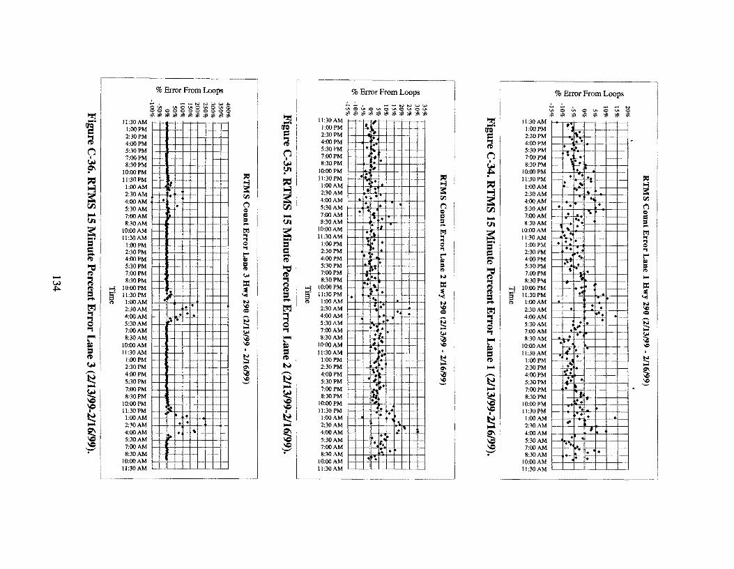
% Error From Loops % Error From Loops % Error From Loops - I --NNWW~ -- . - .... NN l.Ht.W

. - "' OVt V\OVtOV'IQV\Q V\QVlOV\OVIOV\OU'I ..... 0 ~ 0 v. 0 ..... 0 OOOOOOOOQOQ

~ ""<!! ;jl ;jl <ll l!ll <!! <jl ;,11 <II <II ~ ;fl ;fl <II ;j<"""" """" <!! <l'l <II ;j< ;j< "" ;j< ""

<!! "" "" .... ll:30AM 1- , __ -

-~ ~'-·· ~f-- .... 11:30AM I-+·· ~ ll:30AM --+--t

~ l1Cl l:OOPM 1- t.;: .... l:OOPM ~~>- l1Cl J:OOPM l11."'

a 2:30PM = 2:30PM •"~ = 2:30PM · 4:00PM ; 4:00PM ~ 4:00PM .~ +-----!---•• C'".l 5:30PM C'".l

5:30PM . -- 5:30PM --- Fl-; ~ I 7:00PM "-~ I 7:00PM f-- - :: . C'".l 7:00PM ~ <...i <...i S:30PM 1--I

8:30PM 8:30PM f--- ~- -- I-'-· <...i • It ':" IO:OOPM ~ IO:OOPM "# :---1-f-- .i:. IO:OOPM --~~ •• .... := 11:30PM := .

11:30PM • := ~ 11:30PM ~ ~~~ ,_ l:OOAM

., '"3 l:OOAM ••• '"3 ~ l:OOAM :_ ~ ~ 1-1- ~ ~

• ! ~ 2:30AM

I 2:30AM

~ 2:30AM .. ~ I- - r.fl .. • r.fl •. "- __ f.-, __ r.fl 4:00AM

__ ...!_

("'} 4:00AM • ,·-f--f-- 4:00AM r;r., • r;r., 5:30AM • ("'} 5:30AM ,____! • . . ("'} 5:30AM Q I ....... Q r;r., ...... Q ,.... 7:00AM f--~~ = ,.... 7:00AM

' .. ,. -- = ~ 7:00AM 1---- -:-- •• = 01 S:30AM = 01 8:30AM f-- = 01 8:30AM 1--1 -+ = .... I, • ... .... • ....

~ IO:OOAM ~~ l'-!l

~ IO:OOAM ... 1---f-· erJ ~

lO:OOAM I-- erJ ll:30AM

., 11:30AM ., 11:30AM . .. ., .... ., • • ., ~

• --- ~1---- ., = Q l:OOPM ....

l:OOPM ~ l:OOPM Q = -.-l-'-- ___ L.,___ Q

= .,

= 2:30PM . . ., 2:30PM •• .,

2:30PM ~-- t"" . ~ = ;- 4:00PM ..... 4:00PM !:"' ;- 4:00PM ~ '-~

!:"' Ill ~ Ill ~ ~ --- ---- ~ Ill 5:30PM Cl 5:30PM I+ • = 5:30PM • = ~ 1-1- ~

~ 1-- f--

II> 7:00PM . ~· II>

~ * r• • • II> ~ 7:00PM

""' ••• - f-- f--

N 7:00PM , .... - ri w 8:30PM = ~

8:30PM .. .. = "1 8:30PM . = IO:OOPM >-l !O:OOPM f') 10:00 PM I+ • la

.i:.. ~ ::l :I! , __

:I! >-l ~ = 11:30 PM .,_

'-<! ~- ll:30PM • ~ 13· 11:30PM •• . s ~ 1--~~ • '-<! = ,. • ~ ..... ..... •• . . ... l:OOAM -~ ~~ N l:OOAM N ..... ... l:OOAM N

~ ~--' ~· IC

I ~ 2:30AM

4 •• IC ~ L...J • • IC 2:30AM ~~ Q .. Q 2:30AM '-- ~ r;,;r. =

~ 4:00AM ~-

.. , . ,-. =I 4:00AM -··· a 4:00AM . "'"' • ---5:30AM

.... N 5:30AM - . lo_ >- .... N 5:30AM • ,. N ....... 0 - -7:00AM .... "1 7:00AM • .....

7:00AM . ~· .... ~-f--~

~ ·~. Ir "-·· -~

""' "1 •, ""' t"-4 8:30AM '---~ ··- t"-4 8:30AM >-- \Cs 8:30AM . • \Cs IC 1; ~ r- ;r,•' IC • = IO:OOAM = IO:OOAM IC = !O:OOAM '-,,.• 1>-- -· "° = I

= ll:30AM • • . . I 11:30AM _,_ '-'- 1-+- 1-t-- - f-- = 11:30 AM

~ N ~ • N • • N l:OOPM ;::i l:OOPM f-- I-- h1i f+- f-- -- -r--- "·- ....... ~ l:OOPM - ... -<...i N ..... ..... 2:30PM 1-1- 0- ~-1- 1-- 1----1-- °' 2:30PM >-- 1-r,:. -- --t-~

°' ,.... 2:30PM $ - 4:00PM ~ - 4:00PM ~ :;a - 4:00PM

... -- ,__

'--

~ 5:30PM ~ ~ 5:30PM - -_1[.,i IO----- -- ~ ~ 5:30PM !+ • IC

'-" 7:00PM

,.... 7:00PM i.• ,.... 7:00PM • - ----~

~ 8:30PM ~ 8:30PM ~- ~ 8:30PM ~- --LI i.--\Cl \C • ~ IO:OOPM IO:OOPM . -- ·-·- \C IO:OOPM 1 ... \Cl 11:30 PM

;p \Cl 11:30PM . \Cl 11:30PM ..__ ~ ~ I I i. • I

~ l:OOAM . ~ l:OOAM .

~ l:OOAM • I I . --

~11"'" ,___~ • • ,.... 2:30AM 1-l-- ,.... 2:30AM f-- - 1- ,____,. ·->- ,.... 2:30AM - IT ~ 4:00AM I~ $ 4:00AM • e-.. 4:00AM \Cl 5:30AM

...... ~!So 5:30AM l> • It

~ 5:30AM • . . ~ .- 1; • •• t ... \Cl 7:00AM "" 7:00AM \C 7:00AM ':-' ':-' • • • ':-' • 3• 8:30AM ·-- 8:30AM 8:30AM ·"' ~· IO:OOAM ·--~ IO:OOAM • IO:OOAM

11:30AM ~- ~~ 11:30 AM 11:30 AM

t u ] ~

~ ~

i u ] ~ ... j

~

600 560 520 480 440 40 0 360 320 280 240 200 160 120

80 40

0

11 :00 l 2 :30 2 :00 AM PM PM

15 Minute Counts Lane lHwy 290 (219199 • 2/10/99)

3:30 s :00 PM PM

6:10 PM

9:30 PM

11:00 12:30 PM AM

Time

2 :00 AM

J :30 AM

s :00 AM

6:30 AM

8 :00 AM

9:JO AM

ll AM

Figure C-37. Raw Data Plot Lane One (2/9/99- 2/10/99).

15 M inote Counts Lane 2 Hwy 290 (219199 • 2110199)

640 600 560 '20 480 440 400 360 320 280 240 200 160 120

80 40

0

11 :00 12:30 2:00 3:30 5:00 6 :30 8:00 9:30 11:00 12:30 2:00 3:30 5:00 6:30 S:OO 9:30 11:00 AM PM PM PM PM PM PM PM PM AM AM AM AM AM AM AM AM

Time

Figure C-38. Raw Data Plot Lane Two (219199 - 2/10/99).

680 640 600 560 520 480 440 400 360 320 280 240 200 160 120

80 40

0

I

k""1I ·, ...........

.... ~ ...

~

15 Minute Counts Lane 3 Hwy 290 (219199 • 2110/99)

I I I --' l -; I ... ... -.-... - - ··- "'

• :- ·'"' .... - 1·· : .. I -·-

"' ~

~ -- .. ... ,~ - -I ... - - " ·- ...;

I

11:00 12:30 2:00 3:30 s:oo 6:30 8:00 9:30 11:00 12:30 2:00 3:30 5:00 6:30 8:00 9:30 11:00 AM PM PM PM PM PM PM PM PM AM AM AM AM AM AM AM AM

Time

Figure C-39. Raw Data Plot Lane Three (219/99 - 2/10/99).

135

!I c 5 u 3 ,;: ,... ~

...j

i u g "" "" ~

15 M lnute Counts Lane l Hwy 290 (2110199 - 2111/99)

~ ~~ I I i

5 20 +----f..----+-- --+- _...,---+----+- -t----l---+---1:-+----1----11-~~ ..--+:---;: ::~ +----~--+---+----+--------+---+:--..+- ·---!---+-'--''---·-+---:~~--~ ~~--+----:

m ·-- ._ :-:_ lti L ..... _.;._--f-----L '··---r---+:······-·······-+-- --fi~ """-+-~ -.-f .. ~ .... 280 - ·-":iii"" i .. ... ~

f g . -+----+----... -.... -~- ~ :--+---:c- -+--~~"';----r--. +···-----t

80 ~~I WI ~-··b:. 4 ~ 41 ---+--4~----=--=-·~~_····_···~.:~~~.~-~.~.c~--:-:_._--_.J---.... ··_···-+-1 -·······->-----+---+--4~----+---4---+-·--+ 11:30 1:00 L30 4:00 5:30 7:00 8:30 10:00 11:30 t:OO 2'30 4100 5;30 7;00 8:30 10:00 AM PM PM PM PM PM PM PM PM AM AM AM AM AM AM AM

Time

Figure C-40. Raw Data Plot Lane One (2/10/99 - 2/11/99).

15 Minute Counts Lane 2 Hwy 290 (2110199 - 2111199)

600 560 '20 480 440 400 HO 320 280 240 200 160 120

80 40

0

11:30 l :00 2 ;30 4:00 5 :30 7;00 8:30 10:00 11:30 1:00 2:30 4:00 5:30 7:00 8;30 10:00 AM PM PM PM PM PM PM PM PM AM AM AM AM AM AM AM

Time

Figure C-41. Raw Data Plot Lane Two (2/10/99 - 2/11/99).

ISM lnute Counts Lane 3 Hwy 290 (2110199 - 2/11/99)

680 640 600 560 520 480 440 400 360 320 280 240 200 160 120

80 40

0 I l :30 I ;00 2 :l 0 4:00 5 :30 7:00 8:30 10:00 11:30 1:00 2:30 4:00 5;30 7:00 8:30 10:00 AM PM PM PM PM PM PM PM PM AM AM AM AM AM AM AM

Time

Figure C-42. Raw Data Plot Lane Three (2110/99 - 2/11/99).

136

15 Minute Connls Lane 1 Hwy 290 (2111/99 · 2/13/99)

600

$60

<%0

••• l!i 440

" 8 •oo ... '3 320

{?. 280 - 240

" § ..J

120 80

•• ~ f f f f f f f f ~ ~ ~ ~ ~ ~ ~ ~ f f f f f il' f f ~ ~ ~ ~ ~ ~ ~ : ~ iii 8 ~ g g 8 ~ ~ ~ ~ :r; ~ ill ~ :l 8 ~ ~ ~ ~

g 8 :;; ! g 8 ~ ~ " 8

"' . ~ ;! :: - ~ - ~ "' :: ;; . " ~

Time

Figure C-43. Raw Data Plot Lane One (2/11/99 - 2/13/99).

15 Minute Counts Lane 2 Hwy 290 (2/11/99 • 2/U/99)

f f f f f "' f f ~ ~ ~ "' ~ ~ ~ ~ f f f ~ t f f f ~ ~ ~ ~ ~ ~ ~ 0, < ~ iii ! ~ ~ g

~ ~ § ~ ~ ~ ~ c

~ ~ ~ ~ ~ ~ :;; 8 ~ 8 ~ ~ ~ ~ ~ ~ " ~ " :if " $! ~ § -Time

Figure C-44. Raw Data Plot Lane Two (2111/99 - 2/13/99).

lS Minute Counts Lane 3 Hwy 290 (2/11199 · 2113/99)

Time

Figure C-45. Raw Data Plot Lane Three (2/11/99 - 2/13/99).

137

fl = " 0 u ;;;

~

~ -l

15 Minute Counts Lane 1 Hwy 290 (2113/99 • 2/16/99)

600

560

'20

400

440

••• 360

320

zso 240

200

160

120

80

·: .~.. . i-+ +-+-.+=-+·-+I -+--l--l-+--l--+-l--+--1--l-+.-+--f--+-+-+-+-+--l ~ t t t t t l l t ~ ~ ~ ~ ~ ~ ~ ~ l l l t l l l l ~ ~ ~ ~ ~ ~ ~ ~ l l l t l l l l ~ ~ ~ ~ ~ ~ ~ ~ § ~ ! ~ ~ ~ ~ ~ ~ ~ ~ ~ ! : ~ ~ ! ~ ~ ~ ~ ~ ~ ~ ~ ~ ! ~ ~ : ~ ~ § ~ ~ ~ ~ : ~ ~ ~ ~ ~ ~ ~ ~ ~

Time

·-···--··--··--··--~··-···--··--·····-·-···-----... ___ ]

fl = " 0 u

l "' " = ::l

g 5 u !i ~ "' ~

Figure C-46. Raw Data Plot Lane One (2/13/99-2/16/99).

15 Minute Counts Lane 2 Hwy 290 (2/13/99 - 2/10/99)

600

560

520

480

440

400

360

310 280

240

200

160

IZO

•• 40

Time

Figure C-47. Raw Data Plot Lane Two (2/13/99-2/16/99).

15 Minute Counts Lane 3 Hwy 290 (2113/99 - 2116/99)

640

••• '60 ,,. 480 440 400 360 320 280 240 200 160

IZO

•• ~ l l l l l l l l ~ ~ ~ ~ ~ ~ ~ ~ l l l l l l l f ~ ~ ~ ~ ~ ~ ~ ~ f l l l l l f l ~ ~ ~ ~ ~ ~ ~ ~ ~ ~ ~ ~ ~ ~ ~ ~ ~ ~ ~ ~ ~ ~ ~ ~ ~ ~ ~ ~ ~ ~ ~ ~ § ~ ~ ~ ~ ~ ~ ~ ~ ~ ~ ~ ~ ~ ~ ~ ~ ~ ~ ~ ~ ~ ~

Time

Figure C-48. Raw Data Plot Lane Three (2/13/99-2/16/99).

138

11.0 APPENDIX D

SPECIFICATION FOR VIDS DETECTORS

139

TEXAS DEPARTMENT OF TRANSPORTATION SPECIAL SPECIFICATION

VIDEO IMAGE DETECTION SYSTEMS

1.0 GENERAL

This specification sets forth the procurement, installation, and performance requirements for a Video Image Detection System (VIDS) that monitors vehicles on a roadway via processing of video images and provides detector outputs to a traffic controller or similar device. Applications for VIDS include freeway mainlanes, freeway ramp metering, and traffic signal applications.

The VIDS to be supplied shall consist of a data gathering system using the analysis of video images to detect, count, classify, sense speed, etc., of motor vehicles and to generate alarms for certain abnormal conditions. Components comprising the VIDS include, but are not limited to, camera image sensor(s), VIDS processing unit (VPU), computer server hardware, configuration computer hardware and software interface, and graphic user interface.

The VPUs shall communicate asynchronously to a serial expansion device located as described in the plans and that shall communicate by an Ethernet and TCP/IP (transmission control protoco11Internet protocol) connection to VIDS server(s) provided under the contract. The VIDS server(s) shall communicate by an Ethernet and TCP/IP connection to the TXDOT client server using a designated functional output protocol.

The system shall be composed of these principal items: the sensor unit(s), the VIDS processing unit (along with any PC, monitor, or associated equipment required to set up the VIDS), and the field communications link between the sensor unit and the VPU. If required by the plans, a central control along with a remote communications link between the VIDS and central control shall also be supplied.

1.1 Deitnitions

1.1.1 Central Control

Central control is a remotely located control center that communicates with the VIDS. The VIDS operator at the central control has the ability to monitor the operation and modify detector placement and configuration parameters. The equipment that constitutes central control includes a workstation microcomputer along with the associated peripherals, as described in this specification. The location of the central control, if required, will be shown on the plans.

141

1.1.2 Occlusion

Occlusion can occur in either of two ways. The first is when the view of a vehicle in the detection zone is blocked or obstructed from the sensor by another vehicle. This type of occlusion can result in a missed count. The second type of occlusion occurs when a vehicle in one lane enters the detection zone of an adjacent lane. This type of occlusion results in single vehicles being counted in more than one lane. In verification tests of accuracy, occlusion shall be considered as follows. In instances in which a vehicle has been significantly occluded (with respect to a camera's field of view) by another vehicle, that vehicle's count shall not be used in the calculation of the overall accuracy. For purposes of this test, "significant occlusion" defines a target vehicle's image that has been occluded by more than 50 percent.

1.1.3 Supervisor Computer

The supervisor computer is a portable microcomputer used to set up and monitor the operation of the VIDS processor unit. If required to interface with the VIDS processor unit, the supervisor computer with the associated peripherals described in this special specification and a video monitor, also described in this special specification, shall be supplied as part of the VIDS.

1.1.4 Field Communications Link

The field communications link is the communications connection between the sensor unit and the roadside cabinet where the VPU is located. The primary communications link media may be coaxial cable or fiber optic cable.

1.1.5 Remote Communications Link

Remote communications link is the communications connection between the VIDS processor unit and the central control.

1.1.6 Sensor Unit

The sensor unit is the complete camera or optical device assembly used to collect the visual image. The sensor unit consists of a charged coupled device (CCD) camera, environmental enclosure, temperature control mechanism, and all necessary mounting. Power to the sensor unit shall be provided by a three (3) conductor sensor unit power cable, or appropriate cable as approved by the engineer.

1.1. 7 Detection Zone

The detection zone is the area selected through the VIDS processor unit that when occupied by a vehicle, sends a vehicle detection to the freeway management system.

142

1.1.8 Detection Accuracy

Detection accuracy is the measure of the basic operation of a detection system (shows detection when a vehicle is in the detection zone AND shows no detection when there is not a vehicle in the detection zone).

1.1.9 Live Video

Live video is defined as video being viewed and/or processed at 30 frames per second.

1.2 VIDS Configuration

A VIDS configuration wi11 consist of the following components: Four (4) camera sensor units (unless otherwise specified in the plans), one (1) workstation microcomputer with all associated peripherals (if central control is required by the plans), and all associated equipment required to set up and operate in a field environment (field PC or video monitor). The actual quantity and proposed location of equipment to be furnished, installed, and made fully functional, as a complete VIDS, by the contractor will be shown on the plans.

1.3 System Software

The system software shall be able to detect either approaching or receding vehicles in multiple traffic lanes. User-definable detection zones, sufficient to cover up to five (5) lanes and two (2) shoulders shall be available to the user through interactive graphics in an image on a video or VGA monitor. The number and format of detection zones shall be sufficient to determine the parameters and accuracy requirements specified in Section 3.0. The user shall be able to redefine previously defined detection zones.

2.0 VIDS FUNCTIONAL REQUIREMENTS

2.1 Functional Detection Requirements

The VIDS shall be capable of performing the following functions:

• vehicle counting, • vehicle speed measurement, • vehicle classification, and • either individual vehicle data or parameter summaries of 10 seconds or greater.

143

2.2 Functional Output Parameters

The VIDS shall output the following functional detection parameters:

• Volume-vehicles per hour total all lanes. • Speed-time mean and space mean vehicle speed in mph or km/h. • Occupancy-lane occupancy measured in percent of time. • Flow Rate- number of vehicles detected during a specific time interval ( < I hr). • Headway-average time interval in seconds between vehicles passing a fixed point

along the roadway. • Level of Service (LOS)-an expression of the flow rate measured in LOS A through

F, with A being freely flowing traffic and F being forced flow, stop and go conditions. Level of service shall be calculated by the flow rate or occupancy of the lane, with user-definable thresholds for each LOS and the default being defined by the current edition of the Highway Capacity Manual.

• Vehicle Classification-number of vehicles in each of at least three categories: 1) automobiles/vehicles less than 25 feet long, 2) single unit trucks greater than 25 feet long and less that 45 feet long, and 3) tractor-trailer trucks longer than 45 feet.

• Alarm-a function where output is triggered when an abnormal situation is detected (such as continuous presence on a detector or a detection against the flow of traffic), used to warn operators of wrong way vehicles or stopped vehicles.

2.3 Functional Output Protocol

The VIDS server(s) shall provide a high-level interface between Windows applications and the VIDS processors. The VIDS output protocol shall be network-independent and shall allow communication with the TxDOT client server through a high-level TCP/IP network protocol interface via stream sockets. The TxDOT client server shall be able to open up more than one connection with the VIDS server (e.g., open one connection to perform real-time VPU request, and open another connection to receive polled data from the VIDS server). Once a connection has been opened, the TxDOT client server shall be able to open one or more VPUs, including all of the VPUs, and to subsequently request specific data or receive regular polled data. The VIDS server shall be able to process polling requests from the TxDOT client server to maintain a minimum of 20 second polling cycle which shall contain the full complement of detection parameters described in Subsection 2.2. The VIDS server shall, in the event of any disconnection between TxDOT client server and VIDS server, provide error handling capability for automatic reconnection between TxDOT client server and VIDS server without manual intervention.

2.4 VIDS Operating Locations

Two general types of locations exist in which the VIDS system and video camera will be installed. For purposes of this specification, these locations have been identified as

144

Category I and Category Il A Category I installation is a local site installation where monitoring conditions are not conducive to optimal performance (e.g., mounted greater than 10 feet from the shoulder and monitoring multiple traffic lanes from an oblique angle). A Category II installation is a local site installation where monitoring conditions are deemed to be conducive to optimal performance (e.g., an overhead camera installation at optimal height and field-of-view). Category I will be the typical application forTxDOT.

2.4.1 Category I Location

A Category I location is defined as an installed position that does not overlook the roadway directly. The video camera sensor is mounted on a support that is at least 30 feet above the roadway and whose nearest distance from the roadway (shoulder or emergency lane) is at least 10 feet. The video camera sensor shall be equipped with a lens to match the width of the road and aimed to minimize lane vehicle occlusion. The mounting height will be at the top of the specified pole or structure for that location as shown on the plans.

2.4.2 Category I Test Location

The video detection system shall reliably detect vehicle presence in the optimum field of view. The optimum field of view is defined as the sensor's view when the image sensor is mounted 30 feet or higher above the roadway, when the sensor unit is adjacent (within 20 feet) to the edge of the roadway, and when the length of the detection area is not greater than ten (10) times the mounting height of the image sensor. Within this operating field of view, the VIDS processor unit shall be capable of configuring at least a single detection zone for each lane. A single sensor unit, placed at the proper mounting height with the proper lens, shall be able to monitor five (5) traffic lanes plus two (2) shoulder lanes simultaneously.

2.4.3 Category II Location

A Category II location is defined as an installed sensor position directly over the roadway. The video camera sensor is mounted such that it is within 5 feet of the overall center of the lanes to be monitored. The video camera sensor shall be equipped with a lens to match the width of the road and aimed to minimize lane vehicle occlusion. The mounting height will be at the top of the specified pole or structure for that location as shown on the plans.

2.5 Demonstration and Test Requirements

The proposed VIDS equipment or software will be subject to the following criteria.

145

2.5.1 Demonstration

Once the certification documentation has been confirmed and the TMC staff has delivered a letter of approval of the certification, the VIDS manufacturer and/or supplier shall demonstrate and operate a test system. Demonstration and operational performance verification of said system equipment and software (or sub-components) will be on a site designated by TxDOT or their representative and will be conducted in the presence of TxDOT personnel or their representatives. The demonstration requires a Category I field installation, unless stipulated otherwise by the plans. The demonstration shall encompass:

1) Operational test field processor to the VIDS server equipment and software (to be supplied by the manufacturer in accordance with Section 10.0) temporarily installed at a designated TxDOT facility, detecting freeway traffic under existing weather conditions and reporting, through existing data links, to the VIDS server software at theTMC.

2) Operational field test, as in 1) above with the addition of the data links between the VIDS server and TxDOT' s system software, will be performed when the initial operational test is successfully completed.

The locations for the Category I test installations shall be determined by the Department, and Department personnel may also select a site for Category II testing as well. For purposes of simplification of installation and testing, the Department may, at its discretion, choose a freeway location at which a Category I and Category II camera installation can be accomplished simultaneously. If the Department chooses to allow the demonstration to be performed at a currently instrumented site using existing communication links and installed cameras, the equipment vendor shall concur with the use of the existing Department equipment. Otherwise the equipment supplier/manufacturer shall provide all required equipment, installation, setup, and calibration to effectively perform the demonstration.

The initial operational video camera sensor to field processor to VIDS server demonstration test shall last thirty (30) days. At the beginning of the initial thirty (30) day test period, the manufacturer or supplier shall submit catalog cut sheets of the individual components for approval. Results shall be compared to performance specifications identified in Subsection 3.0 prior to the Department granting approval to begin the second testing phase, including the initial field equipment to VIDS server and the VIDS server to the TMC client software process. Once the initial test period has concluded, the Department will either approve or reject the product based solely on the first performance test.

Upon notification of the successful completion of the VIDS server test, the manufacturer will provide the VIDS server output protocol to the Department within 30 calendar days, or liquidated damages in the amount of $500 per day will be assessed until the protocol has been received by the Department. The Department will provide the software

146

expertise to write the required client software to accept the data from the VIDS server and verify the ability to receive the required data in an acceptable form and in the required polling times. The Department will provide the client software 60 to 90 calendar days from the date the vendor protocol information is provided to the Department.

When the Department notifies the manufacturer/supplier that it has completed the software necessary to perform the VIDS server-to-TMC-client portion of the testing, the Department will provide software expertise for a period of 10 consecutive working days to modify and debug the application programming interface (API). Should the interface not be operationally acceptable at the end of this 10 working day period, liquidated damages in the amount of $500 per day will be assessed until the Department has determined that the interface is acceptable.

Once the Department has determined that the VIDS server-to-TMC-client interface is operational, a 10 working day test period will begin. During this period, the Department will determine if the data are being received from the VIDS server in the proper format and at the required polling intervals. Any failure of the VIDS server-to-TMC-client during this 10 working day test period that is attributed to the protocol information provided by the manufacturer/supplier or the VIDS server will constitute failure of the test, and the test will be restarted within 5 working days. If the test fails a second time, liquidation damages in the amount of $500 per day will be assessed until the test is completed successfully. If the test is not successfully completed within 30 days of the second failure, the system will be rejected.

The entire demonstration shall be completed and coordinated within the roadway construction project so that when the prime contractor is ready to open the roadway to traffic, the surveillance system will be in place. This is irrespective of whether the roadway has the final asphalt course applied or not. The VIDS system shall be complete and functional to the extent that the TMC staff can monitor the roadway. Department personnel shall be available to monitor compliance with specification requirements while the system is being tested by the vendor. Testing results shall be in accordance with accuracy specifications described in Section 3.0.

2.5.2 Acceptance Test

Performance of an acceptance test after system installation shall be required. Prior to the Department's acceptance of the installation of the VIDS, the vendor shall perform the acceptance test under observation by Department personnel. The acceptance test shall last at least 30 days, commencing on a date to be specified by the Department, and the VIDS performance shall meet the accuracy requirements stipulated in Section 3.0. The acceptance shall consist of performance testing equivalent to the test performed during the demonstration described in Section 2.5 .2. The acceptance test shall be performed using the installed VIDS, monitoring 100 percent of the roadway presence detection system locations, 10 percent of the Category I and 10 percent of the Category II

147

installations (if required by the plans). Category I and II locations will be determined by the Department. Compliance with specification requirements shall be tested by the vendor in accordance with accuracy specifications described in Section 3.0 under observance by Department personnel. The vendor shall prepare a written report of the results of the test and submit the report to the Department within fourteen (14) calendar days of the completion of the test.

3.0 VIDS FUNCTIONAL ACCURACY REQUIREMENTS

The VIDS functional detection outputs identified in Subsection 2.2 shall meet overall accuracy requirements specified herein under the following environmental and installed location conditions:

• during both day and night periods and transitions from dark to daylight to dusk, • under all weather conditions normally experienced in the local area (if not specified,

bright sunlight to one (1) inch per hour rainfall), and • Category I locations.

Accuracy specifications for the fundamental functional detection parameters listed in Subsection 2.2 are presented below. Detection parameters that are computational derivations of the fundamental parameters (e.g., percentage calculation, etc.) are also discussed. Testing to determine and verify their accuracy shall be conducted for at least two separate four-hour periods which encompass a transition from night-to-day (dawn) and day-to-night (dusk), except as may be amended by the accuracy specifications and measurement conditions described for each parameter below. These four-hour periods will be chosen to evaluate worst case conditions including peak traffic and sun blindness intervals. Additional testing requirements specific to a particular detection parameter are individually discussed. The following specified accuracies are stated as the minimum acceptable values.

3.1 Volume

Average vehicle count during a testing period shall have a 90 percent overall accuracy in Category I locations and 95 percent overall accuracy in Category II locations. These accuracies shall be accomplished with traffic volume of at least 500 vehicles per hour per lane (VPHPL) during off-peak periods and over 1,000 VPHPL during peak periods. Verification of compliance with the accuracy requirement shall be confirmed by performance of a video tape recording (and/or manual or mechanical count confirmation) that pass through each video camera sensor's FOV.

3.2 Speed

Average vehicle speed throughout the detector's FOV shall meet an overall accuracy of 85 percent for Category I locations and 90 percent in Category II. These accuracies shall

148

be valid for traffic moving at speeds between 10 and 75 mph. This test shall be conducted either through the use of video taping equipment or via other electronic methods (e.g., radar detectors used as a speed standard) at the Department's discretion. The tests shall be conducted at three range speeds: 1) slow congested traffic which occurs during rush hour (10-30 mph), 2) moderate traffic flow during non-rush hour conditions (30-50 mph) and 3) unimpeded traffic flow (50-75 mph). Additionally, the testing shall be accomplished for these three speed ranges for both day and night time conditions.

3.3 Occupancy

Lane occupancy calculation for each defined detector within a video camera sensor's FOV shall have an accuracy of 85 percent accuracy for Category I and 90 percent in Category IL Verification of accuracy shall be accomplished using a video tape recording or other electronic methods as used for speed accuracy determination.

3.4 Flow Rate

Flow rate determination shall be equivalent to accuracies f85 percent accuracy for Category I locations and 90 percent for Category II) required for volume determination with detection.

3.5 Headway

Headway accuracy shall be 85 percent for Category I locations and 90 percent for Category II. Verification of headway determination accuracy shall be considered valid when volume, speed, classification, and occupancy accuracies have been tested and determined "within specification" and the vendor has provided certification of the headway calculation to the Department. For purposes of this test, the vendor certification shall contain a detailed description of the headway occupancy calculation to include all pertinent calculation variables.

3.6 Level of Service

Level of service shall be determined with 85 percent accuracy for Category I locations and 90 percent for Category II. Verification of level of service calculation shall be considered valid when occupancy and flow rate determination accuracies have been tested and determined "within specification" and the vendor has provided certification of the level of service threshold calculation to the Department.

3.7 Alarm

The VIDS shall detect wrong-way and stopped vehicles to at least 90 percent accuracy for Category I locations and 95 percent for Category II for each defined detector within a camera image sensor's FOV. Verifications of accuracy compliance shall be conducted

149

using a test vehicle located on a shoulder/emergency lane. The verification test shall be conducted for both day and night time periods lasting at least one hour each. For safety purposes, the Department may elect to only test stopped vehicle detection or to test wrong way detection at a slower speed within the confines of the shoulder/emergency lane detector as traffic conditions permit.

4.0 VIDS EQUIPMENT AND SOFTWARE FUNCTIONAL REQUIREMENTS

Certain major functional capabilities will be required for use of particular VIDS equipment and software in addition to the functional output requirements for the VIDS system as a whole. These features and capabilities include, but are not limited to, the following features/capabilities that directly affect the overall operational performance and goals for the VIDS system.

4.1 VIDS Server Software and Client Applications

The software shall include provision for setup, control, and alarm reporting of multiple abnormal traffic conditions and stopped-vehicle detection zones over a wide area from multiple locations. The VIDS server software shall allow client reconnection without the necessity of a manual restart of the VIDS server process. Each VIDS server software licensed package shall be capable of communicating simultaneously with multiple TxDOT client server processes.

4.1.1 VIDS Equipment

To provide for quick detection of faults, abnormal conditions, and/or traffic related events on an economical basis, the VIDS equipment shall have the ability to process and control multiple video camera sensors. In this respect, processing equipment for the video camera sensors shall be as flexible as possible to the local requirements of the site(s) to be monitored. Therefore, the VIDS equipment shall include the ability to interface a minimum combination of at least one through four video camera sensors with each VPU.

4.1.2 VPU Equipment and Software

The VPU equipment shall have the capability to enable the TMC operator to define multiple detection zones within each individual video camera sensor's field of view at the VPU via the configuration software. Because the quantity and type of zones will vary within the FOV of each video camera sensor, flexibility in definition of the zones and response and processing time of each zone is required. Section 9 .0 describes the requirements of the configuration computer located at the TMC and runs the software which provides the operator interface to configure, edit, and calibrate the detection zones.

150

5.0 VIDS EQUIPMENT AND SOFTWARE TECHNICAL REQUIREMENTS

This VIDS specification sets forth the minimum requirements for system equipment and software that monitor vehicles on a roadway via processing of video images and provides detector outputs to storage or other similar devices such as a video recorder or display unit.

The equipment image communications scheme, beginning at individual video camera sensors to be located throughout the highway system and extending to the VIDS VPU, which shall be installed in satellite building(s) is a single or multi-mode fiber sub-trunk, as indicated in the plans. Potential offerors shall be required to provide and install VIDS video camera sensors on freestanding poles, bridge overpasses, and/or other structures as indicated in the plans. Video signals shall be carried from the camera to the pole­mounted junction/splice cabinet via coaxial cable, then to the VPU via multi-mode fiber optic cable. The data and video outputs from the VPU will then be transmitted multiplexed to a central control point via the single-mode fiber optic trunk cable system.

5.1 System Hardware

The system equipment shall consist of multiple VPUs, each having the capability to input from one to four video camera sensor(s) and/or other video source(s), such as videotape inputs, to a configuration computer. The VPUs and video camera sensors shall be installed at the locations specified in the plans by the provider using the equipment, enclosures, and procedures identified by specifications.

5.2 System Software

The system shall be able to detect either approaching or receding vehicles in multiple traffic lanes. The maximum number of lanes to be monitored by each sensor is five plus two shoulder/emergency lanes. The software shall have the capability to define detectors in each lane and on the shoulders. With a VPU capable of handling from one to four video camera sensors, there shall be sufficient zones to monitor parameters noted for one to four video camera sensors, respectively, that can be user-defined through interactive graphics by placing lines and/or boxes in an image on a VGA monitor. The user shall be able to redefine previously defined detection zones. The VPU shall calculate traffic parameters and provide local non-volatile data storage for later downloading and analysis.

5.2.1 Video Sources

The VPU shall be able to simultaneously process data and images from up to four (4) video camera sensors or two (2) videotape players. The video shall be digitized and analyzed at a rate of at least 30 times per second.

151

5.2.2 Number of Zones

The VPU shall be able to detect the presence of vehicles using a detection zone in each of up to five lanes and two shoulder/emergency lanes within the FOV of each video camera sensor.

5.2.3 Detector Functions

Different detector types shall be selectable via software and at a minimum calculate the parameters defined in Subsection 2.2. Accuracy shall be as defined in Subsection 3.0. Processed information shall be reported from the VPU by individual lane and by grouping user-selectable detectors together into a "station." A "station" is defined as the grouping of one or more lanes together for the purpose of creating a detector output which reflects the sum (vehicle counts) or averages (speed, length, and other functions) of the parameters from individual detectors which make up the station.

5.2.4 Autonomous Detection

Traffic parameters shall be computed by the VPU without a continuous connection to the configuration computer. It shall be possible to disconnect the configuration computer. The VPU shall then detect vehicles as a stand-alone unit and store traffic parameters in its own non-volatile memory. It shall be possible to operate the video detection system with the configuration computer disconnected.

5.2.5 Detection Compensation

The VPU shall be capable of compensating for camera movement attributable to wind, temperature effects, pole sway, pole expansion, or vibration of the mounting when attached to bridges or other structures. The VPU shall employ an algorithm designed to detect and compensate for the effects of movement of the video camera sensors. The user shall be able to activate this function for each video camera sensor via the configuration computer.

5.3 Data Collection and Storage

5.3.1 Detection Parameters

The VPU shall independently compute the following traffic parameters, as defined in Subsection 2.2, over user-defined time interval durations as defmed in Subsection 5.4.2. Accuracy specifications are provided in Subsection 3.0. The VPU shall be capable of storing these data in remote non-volatile memory:

• volume, • speed,

152

• occupancy, • flow rate, • headway, • level of service, and • vehicle classification.

5.3.2 Interval Duration

The VPU shall be capable of computing and storing all traffic parameters in selectable time intervals of 10, 20, or 30 seconds, and 1, 5, 15, or 60 minutes.

5.3.3 Memory

All traffic parameter data shall be stored in non-volatile memory within the VPU. This data shall be capable of being retrieved using the configuration computer at a later time. Non-volatile memory size shall be at least 4 MB.

5.3.4 Data Retrieval

Transfer of traffic parameter data from the VPU's non-volatile memory to the configuration computer (or other computer) shall be via a serial communications port. Transfer of data shall be by any or all of the following modes: modem and dial-up telephone lines, fiber optic network, or direct connection to another computer.

5.4 Operation with Configuration Computer On-line

5.4.1 Simultaneous Operation

Updating of other VPUs connected to the server shall not be delayed while the configuration computer is on-line and a particular VPU is being viewed. Data from other VPUs must continue to be transmitted to the TMC at a minimum rate of once every twenty (20) seconds.

5.4.2 Storage Format

The configuration computer shall be capable of storing collected traffic parameter data after that data is retrieved from the VPU. This data shall be readily accessible ASCII format. Software on the configuration computer shall provide a means for retrieving, reporting, and filing the collected traffic parameter data.

5.4.3 Data Display Format

It shall be possible to display the collected traffic parameter data of the last complete time interval in numeric format on the configuration computer's monitor. Selecting the

153

data to be viewed shall be accomplishable using pull-down menus or an equivalent Windows graphical interface.

5.4.4 Image Capture

It shall be possible to capture a still image (snapshot) from any of the VPU's active video inputs and download the image to the configuration computer for display for storage as a picture file.

5.4.5 Communications

Communications between the configuration computer and the VPUs shall be via either a direct or multi-drop architecture as described in Subsection 2.3. An error-checking and retransmission protocol shall be employed during file and data downloads and uploads.

6.0 Vehicle Detection Programming Requirements

6.1 Detection Zone Placement

It shall be possible to place vehicle detection zones anywhere within the field of view of the video camera sensors. Detection zones shall be lines or boxes drawn in each visible lane or area of desired detection. Detectors may overlap if necessary. No more than three (3) drawn detection zones per lane shall be required for the VPU to compute all the traffic parameters defined in Section 2.2.

6.1.1 Placement and Manipulation

The configuration computer shall allow the user to draw detection zones through the Microsoft Windows or equivalent graphics environment with a mouse interface. The configuration computer's monitor shall display the detection zones superimposed on the video camera sensor's images.

It shall be possible to create detection zones of varying size and shape to allow best coverage of the viewable roadway lanes, ramps, and shoulders. Once drawn, all the detection zones in a particular video camera sensor image may be saved as a detector file on the configuration computer for immediate or future downloading to the VPU. It shall be possible for the user to retrieve the current active detector file from the VPU.

6.1.2 Detection Zone Editing

It shall be possible to edit existing detector configuration files using the configuration computer. Once edited, the new detector file shall be viewable on the configuration computer's monitor.

154

7.0 VPU HARDWARE REQUIREMENTS

For simplification, standardization, and maintenance purposes, the specifications shall apply to any equipment offered as part of the procurement.

7.1 VPU Environmental

The VPU shall operate reliably in a typical roadside traffic cabinet environment. Enclosures shall meet NEMA 250 Type 4 specifications and internal equipment shall meet the environmental requirements of NEMA TS 1-1989 (R 1994) and NEMA TS2-1992 standards and the environmental requirements for Type 170 and Type 179 controllers. Operating temperatures shall be from -34 to+ 74 degrees C from 0% to 95% relative humidity, non-condensing.

7.2 VPU Electrical

7.2.1 Serial Communications

Serial communications to the configuration computer shall be through RS-232/RS-422 serial port for downloading traffic data stored in non-volatile memory and for receiving detection information. This connector shall be on the front of the VPU for easy access when rack remounted.

7.2.2 VPU Video Input

The VPU shall have one ( 1) to four ( 4) RS-170A black and white composite video inputs such that signals from up to four ( 4) video camera sensors or other synchronous or non­synchronous video sources can be processed in real-time. BNC connectors on the front of the VPU shall be used for all video inputs.

7.2.3 VPU Software

The VPU software shall be stored in a non-volatile memory within the VPU. Software updates shall be performed either through the configuration computer or direct computer communication through a serial port.

8.0 VIDEO CAMERA SENSOR SPECIFICATIONS

This section describes the minimum performance and installation requirements of the video camera sensors to be supplied by the contractor. The contractor shall furnish and install the camera, automatic iris lens, environmental enclosure with sun shield, and all cables and connectors and additional enclosures and associated equipment required to interface the camera unit to the VPU as indicated in the plans.

155

8.1 Video Camera Sensor

The video detection system shall use high resolution, monochrome video camera sensors as the primary video source for real-time vehicle detection. Optical fibers and/or electrical circuitry shall be used in the video camera sensor to compensate for blooming at night caused by headlights and minor vibration caused by wind of vehicle movement on overpasses/bridges to which the cameras are mounted. As a minimum, each video camera sensor installation shall meet the following requirements:

• Video Camera Sensor: 1A inch to 1 inch interline or frame transfer charge coupled device (CCD)

• Active Pixel Elements: 768 Horizontal, 494 Vertical minimum • Video Standards: RS-170A Compliant (available as EIA-170A specification) • Iris: Automatic, with damping. The video camera sensor shall be equipped with an

auto-iris lens with an 4.8 to 48mm motor driven variable focal length lens. Lens adjustment shall take place from outside the pressurized video camera sensor housing. The contractor to the satisfaction of the engineer shall adjust each lens. The aperture shall be pre-focused at infinity, and the aperture size shall be determined by the vendor based on specific site locations and conditions to meet overall detection and accuracy requirements of the VIDS specified in Subsection 1.3.

• Resolution: 580 Horizontal TVL, 350 Vertical TVL • Synchronization: Crystal of AC line lock • Minimum Sensitivity: 0.1 lux at 100% video with no AGC, with 55dB SIN ratio • Dynamic Range: 56 dB minimum (from minimum to maximum useable video

signal) • Automatic Gain Control CAGC): 20dB minimum, 1 second damped. AGC shall not

be applied until automatic iris control has fully opened the aperture. • Gamma Correction: 1.0 required for optimal image processing capability • Adjustments: AGC and automatic iris controls shall be adjusted to provide:

• Black Level: 0 IRE units (-0.3 volts peak video signal) • No-Contrast Image: 50 IRE units (-0.65 volts peak video signal) • 100% Video Level: 100 IRE units (1 volt peak)

The automatic iris shall operate in a damped manner with a time constant of 0.25 seconds or longer.

Input Power: 15 V AC +I- 10%, 60 Hz nominal ±3Hz. Power conductors from the power source to the camera input shall be sized so that no more than a 3% voltage drop is experienced (NEC 210-19a., FPN No. 4). The camera enclosure shall include a provision at the rear of the enclosure for connection of power and video signal cables.

156

Electromagnetic Interface (EMD: FCC Part 15, Subpart J, Class A device requirements apply for the video camera sensor and associated connected equipment in their installed condition.

Video Camera Sensor Enclosure: The video camera sensor shall be provided for installation in a light colored enclosure to limit solar heating. The enclosure shall meet NEMA 250 Type 4 enclosure standards and shall be pressurized to at least 5 psi ± 1 psi to prevent sand, dirt, dust, salt, and water from entering. A sun shield visor shall be affixed to the front of the enclosure which is sufficiently adjustable to divert water away from the video camera sensor lens and also prevent direct sunlight from entering the iris when mounted in its installed location. The sun shield shall not impede operation or performance accuracy of the video camera sensor, nor shall it require removal of the video camera sensor enclosure for adjustment. The enclosure shall allow the video camera sensor horizon to be rotated in the field during installation.

Weight: 10 lbs. maximum with mount, shield, and camera.

Mounting: The video camera sensor assembly and associated enclosure and sun shield shall be capable of being mounted without specific tools, fixtures, or holding devices. The video camera sensor horizon shall be adjustable without removing the camera, mounting bracket and enclosure, or sun shield.

Environmental:

Operating ambient temperature range: -30°F to 140°F. Additionally, a heater shall be installed at the front of the enclosure to prevent the formation of ice and condensation in cold weather, as well as to assure proper operation of the lens' iris mechanism. The heater shall not interfere with the operation of the video camera sensor electronics, and it shall not cause interference with the video signal.

Humidity: 5-95% humidity per NEMA TSl-1989 (R1994)

Vibration: Performance shall not be impaired by vibration when mounted on 80 ft or shorter pole. The video camera sensor and enclosure shall maintain their functional capability and physical integrity when subjected to a vibration of 5 to 30 Hertz up to 0.5 gravity applied to each of three mutually perpendicular axes (NEMA TSl-1989 (R1994)).

157

Shock: The video camera sensor and enclosure shall withstand a lOG-±lG shock. Neither permanent physical deformation nor inoperability of the video camera sensor and enclosure shall be sustained as a result of this shock level.

Acoustic Noise: The video camera sensor and enclosure shall withstand 150 dB for 30 minutes continuously, and their function and accuracy shall not be reduced.

Additional Enclosures: At each installation site, a Type 1 cabinet housing shall be supplied for installation on the structure to be used for video camera sensor mounting. The specification of the cabinet shall be specified in the plans. The traffic cabinet shall contain a terminal block for terminating power to the video camera sensor, connection points for coaxial cables from the video camera sensor, fiber-optic transceivers, and fiber-optic cables connected to/from the VPU in the hub.

9.0 CONFIGURATION COMPUTER SYSTEM

9.1 Windows Software

The configuration computer system shall consist of a computer with Windows-based interface software. This system will be used to configure detection zones and retrieve stored VPU data. For each VIDS and for each PDS system, one complete configuration computer system and a spare (for a total of two complete configuration systems and two spares) shall be provided and located at the TMC or a location specified by the Department.

9.2 Computer Specifications

Minimum specifications for the configuration desktop computer are: • Intel Pentium II Processor 166 MHz or higher with a full-size AT-compatible

expansion slot capability • At least 1 PCI and 1 ISA expansion slot • Microsoft Windows (latest version) or equivalent • 17" minimum VGA color monitor • 8MB, 128 bit AGP graphics adapter • Enhanced keyboard (102 keys minimum) • Serial mouse • 64MB of RAM • 3.5" floppy disk drive • 4 GB or higher hard disk drive • 32x CD ROM or faster • 3COM PCI 10/100 twisted pair Ethernet adapter

158

9.3 Digitizer Board

If a digitizer board is needed, it shall be installed in the configuration desktop computer to support real-time display of video. Still image viewing of video images shall not be a required input into the digitizer board. The digitizer board shall permit viewing of real­time roadway video on the configuration computer's monitor. The board shall fit in a full-size AT-compatible slot within the configuration computer and shall be initially set up by the supplier as necessary for operation with the VIDS.

9 .4 Software

The configuration computer shall include a Windows-based program to interface with any models/versions of the supplied VPU. The software shall provide an easy to use graphical interface and support all models/versions of the supplied VPU. The software shall support either still image or real-time viewing of video images within a window. Still image views shall not require the use of a video digitizer board.

10.0 VIDS Server Computer System

10.1 VIDS Server System

For each VIDS system and each PDS system, one complete VIDS server and a spare (for a total of two complete VIDS server computer systems and two spares) shall be provided and located at the TMC or at a location specified by the Department. All costs associated with the VIDS server computer system shall be paid for under contract pay items, and the Department shall make no separate payment for the VIDS server computer system. The minimum VIDS server system shall consist of the following.

• Dual Intel Pentium II Processors 200 MHz or higher with 512K ECC Cache for each processor.

• Microsoft NT server 4.0 or higher (1to4 CPUs) • 17 inch VGA color monitor • 8 MB, 128 bit AGP graphics adapter • Enhanced keyboard (102 keys minimum) • Serial mouse • 128 MB of RAM • 3.5" floppy disk drive • 8 GB or higher hard disk drive • 32x CD ROM or faster • 3COM PCI 1Oil00 twisted pair Ethernet adapter

159

11.0 INSTALLATION

11.1 VIDS Equipment

The supplier of the video detection system equipment and software shall install all video camera sensors, VPUs, and associated enclosures and equipment at the locations specified in the plans. The supplier is also responsible for test and verification of satisfactory operation of each equipment item prior to acceptance of the VIDS. The installer shall be responsible for making all necessary adjustments and modifications to the total VIDS system prior to obtaining TMC recommendation for system acceptance. Additionally, a factory-certified representative from the VIDS equipment manufacturer/supplier shall be on-site during installation as may be required by the Department.

11.2 VIDS Configuration Computer

In the event that the configuration computer is furnished by the Department, installation of the hardware and provision and installation of the software shall be accomplished by the VIDS equipment and software supplier, and testing shall be done at the time that training is conducted.

12.0 WARRANTY, MAINTENANCE, AND SUPPORT

12.1 Warranty

The complete video detection system equipment and software shall be warranted by its supplier for a minimum of two (2) years. The two (2) year warranty period shall begin when the project has received final acceptance from the Department OR when the prime contractor requests and receives a partial acceptance of the VIDS system from the Department. When the Department detects a failure of any component of the system during the warranty period, the Department shall notify the supplier in writing of the problem. The supplier shall have a maximum of seven calendar days after receiving the notification to correct the problem or liquidated damages in the amount of $500 per day will be assessed until the problem is corrected. The supplier shall repair or replace the defective device(s) and ensure that all vehicle detection affected by the problem is brought within original accuracy parameters. Once accuracy has been verified by the Department, the problem will be considered resolved.

12.2 Maintenance

Normal, routine maintenance (camera lens cleaning, periodic inspections, etc.) shall be performed by Department personnel. However, malfunction conditions which affect overall detection performance which can be attributed to a specific component or item­level components of the VIDS (e.g., VIDS server, VPU, video camera sensor,

160

configuration computer, or software) shall be repaired under warranty at no cost to the Department as detailed in Subsection 12.1.

12.3 Support

During the warranty period, any software upgrades of the VPU and/or configuration management software shall be supplied to the Department at no charge. In addition, phone consultation as needed shall be provided at no cost during the warranty period for operating questions or problems that arise.

12.4 Future Support

H the Department desires, it may enter into a separate agreement with the suppliers for technical support and software upgrades. The supplier shall make available such programs to the Department after the original warranty period.

13.0 MEASUREMENT

13.1 Video Surveillance System Installation

Unless otherwise specified in the plans, a video surveillance system installation shall, at a minimum, include furnishing and installing the following for each site, where a site is defined as a pole or other mounting structure with one or more video camera sensors mounted on it which are all served by the same equipment cabinet:

• Camera(s), environmental enclosure(s), and mounting assembly(ies) with all associated hard ware.

• Equipment cabinet with power service, surge protector(s), communications components, and grounding.

• Fiber optic video transmitter(s) in the equipment cabinet for transmission to the communications hub as specified in the plans.

• Fiber optic video receiver(s) in the specified communications hub for receiving the video from the VIDS site.

• Fiber optic drop kit including, but not limited to, the drop fiber, fusion splice of drop fiber to trunk cable, splice closure, connecting hardware, and conduit to the trunk cable splice location.

• All hardware and materials necessary to provide electrical power service to the VIDS field location as shown in the plans, including, but not limited to, electrical service pole, weatherheads, conduit, conduit risers, conduit hardware, pull boxes, wire, circuit breakers, disconnect enclosures, and grounding.

• All cables, connectors, hardware, interfaces, supplies, and any other items necessary for the proper operation and function of any VIDS system component to carry video signals to the VPU.

161

13.2 Video Detection System Processor

Unless otherwise specified in the plans, a video detection system processor shall include, at a minimum, furnishing and installing the following:

• rack mountable VIDS equipment, and • system software provided within the VPU.

14.0 PAYMENT

14.1 Video Surveillance System Installation

A video surveillance system installation, complete in place and accepted by the Department, shall be paid for at the Per Each Contract bid price.

14.2 Video Detection System Processor

A video detection system processor, complete in place and accepted by the Department, shall be paid for at the Lump Sum Contract bid price.

162

12.0 APPENDIX E

SPECIFICATION FOR MICROWAVE DETECTORS

163

TEXAS DEPARTMENT OF TRANSPORTATION SPECIAL SPECIFICATION

MICROWAVE VEHICLE PRESENCE DETECTION SYSTEM

1.0 GENERAL

1.1 This item shall govern for the rmmmum acceptable design and installation requirements for an overhead/side-mounted microwave vehicle presence detector. All equipment required to interface with a traffic signal controller will be subsidiary to this pay item.

1.2 In side-mount, the unit shall detect the continuous presence, volume, occupancy, and average speed of every type of vehicle that is licensed to date in at least five detection zones.

1.3 The horizontal range for detection shall be from a minimum of 3 m (10 ft) to a maximum of 60 m (200 ft) for a detector unit mounted at a height of 5 m (17 ft).

1.4 The sensor shall be able to hold the detection until the zone is cleared. Additionally, the sensor shall be able to tune-out stationary targets that remain within the detection zone for a minimum of 15 minutes.

1.5 The sensor shall self-tune to its detection zone with no external adjustments other than physical alignment. There will be no external tuning controls of any kind, which will require an operator.

1.6 The detector output must be directly compatible with the controller cabinet detector input.

1.7 The operator shall be able to set up, monitor lane status, and retrieve data from the detector through the RS 232 serial port with any IBM compatible laptop or desktop computer. Also, the detector shall be compatible with a standard phone modem for remote data retrieval.

1.8 The detector shall be capable of continuous operation over a temperature range of -37 to 74 degrees Celsius and relative humidity of 95% non-condensing.

2.0 FUNCTIONAL REQUIREMENTS

2.1 The microwave unit must have Federal Communications Commission (FCC) certification. The FCC-ID number must be displayed on an external label. The detector will operate at a frequency, as allowed under the FCC rules, part 15.

165

2.2 Cabinet power utilized by a detector power supply will range from 95 to 135 VAC as per NEMA TS-1. The detector will be self-contained. If an external power supply is necessary, it shall be supplied as part of the detector system and shall be considered subsidiary to the unit cost of the detector system.

2.3 The unit will have an optically isolated relay contact pair for each detection zone to send a signal to the controller.

2.4 No component shall be of such design, fabrication, nomenclature, or other identification as to preclude the purchase of said component from any wholesale electronic distributor.

2.5 The unit must employ a circuit for power failure to put the relay to a fail-safe position (recall) during a power failure.

2.6 The detector must have a monitoring circuit for the transceiver that will change the output relay to the fail-safe position in the event of a component failure.

2. 7 The detector shall work either as a side of the pole mounted detector for multiple zones or as an overhead mounted detector for a single zone at a height range of 5 m (17 ft) to 10 m (33 ft).

2.8 All setup, controller program, and diagnostic software shall be provided and run on the latest version of DOS- or Windows-based operating systems. Software updates shall be provided free of charge during the warranty period.

3.0 FUNCTIONAL ACCURACY REQUIREMENTS

3.1 The detector shall meet overall accuracy requirements specified herein under the following environmental and installed location conditions:

• under all weather conditions normally experienced in the local area, and • installed in overhead (forward-mounted single lane) or side-mounted (side­

mounted multiple lane) position on a sign bridge.

3.2 Presence accuracy from overhead mount shall be at least 95 percent in a single detection zone. Accuracy in detection and magnitude of speed shall be at least 95 percent from an overhead mount.

3.3 Presence accuracy from a side-mounted position shall be at least 90 percent in multiple detection zones. Accuracy in detection, volume, occupancy, and magnitude of speed shall be at least 85 percent from a side-mounted position.

166

4.0 MECHANICAL REQUIREMENTS.

4.1 Each sensor shall be enclosed in a finished fabricated plastic and aluminum chassis with a minimum 4-inch square high impact plastic opening in front of the antenna.

4.2 Each detector chassis shall be water resistant without the use of silicone gels or any other material that will deteriorate under prolonged exposure to ultraviolet rays.

4.3 The printed circuit board shall be coated with a clear coat moisture and fungus resistant material (conformal coated).

4.4 The sensor shall be furnished with a bracket or band designed to mount directly to a pole or overhead mast-arm or other structure.

4.5 The sensor shall interface with the controller program via a RS-232 port.

4.6 The maximum size of the detector shall be: • Height: 12 inches • Width: 18 inches • Depth: 12 inches

4.7 The sensor shall have a single military style multi-pin connector to provide power and output signals for RS 232 and all contact pairs.

5.0 FUNCTIONAL TESTS

5.1 The manufacturer will test all microwave units to ensure compliance to all FCC and department specifications.

5.2 The manufacturer will be required to supply a medical statement as to the safety of the unit to the general public (example: pacemakers, etc.).

6.0 MEASUREMENT

Each overhead/side-mounted microwave presence vehicle detector in place will measure presence, volume, occupancy, and average speed in each detection zone.

167

7.0 PAYMENT

The work performed and materials furnished in accordance with this item and measured as provided under "measurement" will be paid for at the unit price bid for "microwave overhead/side-mounted vehicle detector (presence)." This price shall be full compensation for furnishing and installing all materials, and for all labor, tools, equipment, and incidentals necessary to complete the work.

168