EVALUATION OF PILOT AND QUADCOPTER PERFORMANCE …
91
EVALUATION OF PILOT AND QUADCOPTER PERFORMANCE FROM OPEN LOOP MISSION ORIENTED FLIGHT TESTING A Thesis IN Mechanical Engineering Presented to the Faculty of the University of Missouri–Kansas City in partial fulfillment of the requirements for the degree MASTER OF SCIENCE by MUHAMMAD JUNAYED HASAN ZAHED B. S., Bangladesh University of Science and Technology, Dhaka, Bangladesh, 2014 Kansas City, Missouri 2018
Transcript of EVALUATION OF PILOT AND QUADCOPTER PERFORMANCE …

EVALUATION OF PILOT AND QUADCOPTER PERFORMANCE FROM OPEN
LOOP MISSION ORIENTED FLIGHT TESTING
A ThesisIN
Mechanical Engineering
Presented to the Faculty of the Universityof Missouri–Kansas City in partial fulfillment of
the requirements for the degree
MASTER OF SCIENCE
byMUHAMMAD JUNAYED HASAN ZAHED
B. S., Bangladesh University of Science and Technology, Dhaka, Bangladesh, 2014
Kansas City, Missouri2018

c© 2018
MUHAMMAD JUNAYED HASAN ZAHED
ALL RIGHTS RESERVED
EVALUATION OF PILOT AND QUADCOPTER PERFORMANCE FROM OPEN
LOOP MISSION ORIENTED FLIGHT TESTING
Muhammad Junayed Hasan Zahed, Candidate for the Master of Science Degree
University of Missouri–Kansas City, 2018
ABSTRACT
Ease of control, portability and efficiency in versatile applications have made Un-
manned Aerial Vehicle (UAV) very popular. Considering various usefulness, safe opera-
tion of UAV is important and to ensure safe operation, proper synergy between pilot and
UAV is mandatory. For this reason, individual evaluation of both pilot and UAV perfor-
mance is vital so that pilot can accomplish a task with the assigned system without any
accident. In this study, a new evaluation technique of pilot and UAV performance is pre-
sented based on flight test results of a mission task of following a desired path. Seven
pilots are categorized into two groups based on their experience level and a quadcopter is
categorized into three groups based on level of autonomy associated with it. Path error
is calculated in time domain to distinguish between pilot levels and level of autonomy of
UAV. Path error metrics show that novice pilots make more error than experienced pilots
iii
and error increases from more autonomous to less autonomous UAV. For frequency do-
main analysis, transfer function modeling is done including human operator in the open
loop so that full scenario of the flight, from pilot to UAV can be analyzed. Frequency
domain analysis helps to identify system complexity, stability and fastness based on level
of autonomy as well as pilot performance based on experience level. Apart from time
and frequency domain analysis, Cooper-Harper rating scale is used by the pilots to rate
the UAV based on ease of control. Along with time and frequency domain variables,
Cooper-Harper rating is included as predictors in the modeling of evaluation of pilot and
quadcopter performance. The parameter estimation of regression model shows the change
in model outcome for both pilot and UAV level with the variation of predictor values. In
the end, a verification test case is included where an eighth pilot flies the same quadcopter
to complete the same task and variables derived from the flight data of this single flight
test are placed in the binary logistic regression model equation to predict pilot experience
level and multinoial logistic regression model equation to predict UAV autonomy level.
The established model can predict pilot experience level and UAV autonomy level cor-
rectly that matches with the real case. The evaluation technique developed in this thesis
shows a path to evaluate pilot and quadcopter performance individually, that can be used
to train pilots to accomplish a specific task with the assigned UAV system.
iv

APPROVAL PAGE
The faculty listed below, appointed by the Dean of the School of Computing and Engi-
neering, have examined a thesis titled “Evaluation of Pilot and Quadcopter Performance
from Open Loop Mission Oriented Flight Testing ,” presented by Muhammad Junayed
Hasan Zahed, candidate for the Master of Science degree, and hereby certify that in their
opinion it is worthy of acceptance.
Supervisory Committee
Travis Fields, Ph.D., P.E. Committee ChairDepartment of Civil & Mechanical Engineering
Gregory W. King, Ph.D., P.E.Department of Civil & Mechanical Engineering
Sarvenaz Sobhansarbandi, Ph.D.Department of Civil & Mechanical Engineering
v

CONTENTS
ABSTRACT . . . . . . . . . . . . . . . . . . . . . . . . . . . . . . . . . . . . . . iii
List of Figures . . . . . . . . . . . . . . . . . . . . . . . . . . . . . . . . . . . . . viii
List of Tables . . . . . . . . . . . . . . . . . . . . . . . . . . . . . . . . . . . . . x
ACKNOWLEDGEMENTS . . . . . . . . . . . . . . . . . . . . . . . . . . . . . . xii
Chapter
1 INTRODUCTION . . . . . . . . . . . . . . . . . . . . . . . . . . . . . . . . . 1
1.1 Significance of evaluating pilot & unmanned aircraft performance . . . . 1
1.2 Evaluation of pilot & quadcopter performance . . . . . . . . . . . . . . . 2
1.3 Goals and Objectives . . . . . . . . . . . . . . . . . . . . . . . . . . . . 5
2 LITERATURE REVIEW . . . . . . . . . . . . . . . . . . . . . . . . . . . . . 6
2.1 Open & Closed Loop System . . . . . . . . . . . . . . . . . . . . . . . . 6
2.2 Human Operator Modeling . . . . . . . . . . . . . . . . . . . . . . . . . 7
2.3 Transfer Function Modeling . . . . . . . . . . . . . . . . . . . . . . . . 9
2.4 Error Metrics . . . . . . . . . . . . . . . . . . . . . . . . . . . . . . . . 10
2.5 Stability Margin Criteria . . . . . . . . . . . . . . . . . . . . . . . . . . 11
2.6 Cooper-Harper Rating Scale . . . . . . . . . . . . . . . . . . . . . . . . 14
2.7 Logistic Regression Modeling . . . . . . . . . . . . . . . . . . . . . . . 15
3 METHODOLOGY . . . . . . . . . . . . . . . . . . . . . . . . . . . . . . . . 18
3.1 Test Arena & Path Planning . . . . . . . . . . . . . . . . . . . . . . . . . 18
vi
3.2 Selection Process of pilot & unmanned aircraft . . . . . . . . . . . . . . 20
3.3 System Configuration . . . . . . . . . . . . . . . . . . . . . . . . . . . . 23
3.4 Time Domain Analysis . . . . . . . . . . . . . . . . . . . . . . . . . . . 25
3.5 Frequency Domain Analysis . . . . . . . . . . . . . . . . . . . . . . . . 28
3.6 Cooper-Harper Rating Scale . . . . . . . . . . . . . . . . . . . . . . . . 31
3.7 Pilot Experience Level Modeling . . . . . . . . . . . . . . . . . . . . . . 32
3.8 Autonomy Level of UAV Modeling . . . . . . . . . . . . . . . . . . . . 36
3.9 Multinomial Logistic Regression . . . . . . . . . . . . . . . . . . . . . . 38
3.10 Verification Test Case . . . . . . . . . . . . . . . . . . . . . . . . . . . . 39
4 RESULTS AND DISCUSSIONS . . . . . . . . . . . . . . . . . . . . . . . . . 41
4.1 Time domain analysis . . . . . . . . . . . . . . . . . . . . . . . . . . . . 41
4.2 Frequency domain analysis . . . . . . . . . . . . . . . . . . . . . . . . . 48
4.3 Cooper-Harper Rating Scale . . . . . . . . . . . . . . . . . . . . . . . . 55
4.4 Pilot Experience Level Modeling . . . . . . . . . . . . . . . . . . . . . . 56
4.5 UAV Autonomy Level Modeling . . . . . . . . . . . . . . . . . . . . . . 58
4.6 Verification Test Case . . . . . . . . . . . . . . . . . . . . . . . . . . . . 62
5 CONCLUSION . . . . . . . . . . . . . . . . . . . . . . . . . . . . . . . . . . 66
6 FUTURE WORK . . . . . . . . . . . . . . . . . . . . . . . . . . . . . . . . . 68
REFERENCE LIST . . . . . . . . . . . . . . . . . . . . . . . . . . . . . . . . . . 69
VITA . . . . . . . . . . . . . . . . . . . . . . . . . . . . . . . . . . . . . . . . . 78
vii
List of Figures
Figure Page
1 Control System (a) Open loop (b) Closed loop . . . . . . . . . . . . . . 6
2 Inpretation of gain and phase margin from bode plot . . . . . . . . . . . . 12
3 Modified Cooper-Harper Rating Scale for Unmanned Aircraft [1] . . . . . 17
4 Schematic diagram of desired path . . . . . . . . . . . . . . . . . . . . . 19
5 Flight test arena . . . . . . . . . . . . . . . . . . . . . . . . . . . . . . . 20
6 Steel rod gates through which the quadcopter is flown by pilots to follow
the desired path . . . . . . . . . . . . . . . . . . . . . . . . . . . . . . . 21
7 Marker used as a starting point and furthest turn around point for UAV . . 22
8 Quadcopter System . . . . . . . . . . . . . . . . . . . . . . . . . . . . . 23
9 Controller and UAV transfer function combined together . . . . . . . . . 28
10 Pilot transfer function . . . . . . . . . . . . . . . . . . . . . . . . . . . 29
11 Combined Open Loop Transfer Function . . . . . . . . . . . . . . . . . 29
12 Visual representation of flight path of each category pilot (a) Level 1 au-
tonomy (b) Level 2 autonomy (c) Level 3 autonomy . . . . . . . . . . . 42
13 Path error diagram of an experienced pilot’s flight (a) Level 1 autonomy
(b) Level 2 autonomy (c) Level 3 autonomy . . . . . . . . . . . . . . . . 43
14 Second order transfer function fitting (a) Level 1 autonomy (b) Level 2
autonomy (c) Level 3 autonomy . . . . . . . . . . . . . . . . . . . . . . 49
viii

15 Fourth order transfer function fitting for Level 3 autonomy . . . . . . . . 50
16 Bode plot of Level 1 autonomy mode . . . . . . . . . . . . . . . . . . . 51
17 Bode plot of Level 2 autonomy mode . . . . . . . . . . . . . . . . . . . 52
18 Bode plot of Level 3 autonomy mode . . . . . . . . . . . . . . . . . . . 53
ix
List of Tables
Tables Page
1 Pilot self rating & experience level . . . . . . . . . . . . . . . . . . . . . 21
2 Specifications of flight controller . . . . . . . . . . . . . . . . . . . . . . 24
3 Abbreviated Cooper-Harper rating scale for UAV tasks . . . . . . . . . . 32
4 Mean value of path error (ft) for each pilot’s flight test in each autonomy
level . . . . . . . . . . . . . . . . . . . . . . . . . . . . . . . . . . . . . 45
5 Standard Deviation of path error (ft) for each pilot’s flight test in each
autonomy level . . . . . . . . . . . . . . . . . . . . . . . . . . . . . . . 46
6 RMS value of path error (ft) for each pilot’s flight test in each autonomy
level . . . . . . . . . . . . . . . . . . . . . . . . . . . . . . . . . . . . . 47
7 Gain Margin(dB) and Phase Margin (degree) for each pilot’s flight test in
each autonomy level . . . . . . . . . . . . . . . . . . . . . . . . . . . . 55
8 Pilot given C-H rating of UAV in different flight modes . . . . . . . . . . 56
9 P value of independent sample t-test for pilot experience level . . . . . . 57
10 Parameter estimation for pilot level modeling . . . . . . . . . . . . . . . 58
11 P value of ANOVA test for flight autonomy level . . . . . . . . . . . . . 59
12 Post hoc test for flight autonomy level . . . . . . . . . . . . . . . . . . . 60
13 Parameter estimation for flight autonomy level modeling . . . . . . . . . 62
14 Model predictors’ values of verification flight test . . . . . . . . . . . . . 63
x
15 Parameters and independent variable values for pilot experience level pre-
diction . . . . . . . . . . . . . . . . . . . . . . . . . . . . . . . . . . . . 63
16 Parameters and independent variable values for UAV autonomy level pre-
diction . . . . . . . . . . . . . . . . . . . . . . . . . . . . . . . . . . . . 64
xi

ACKNOWLEDGEMENTS
Funding was provided by UMKC Strategic Funding Initiatives. I would like to
thank my academic advisor Dr. Travis Fields for his continuous support and ideas during
the research work. Thank you to all the members of Parachute and Aerial Vehicle Systems
Lab and Drone Research and Teaching Lab at UMKC including Mohammed Alabsi, Ig-
nacio Harnandez, Shawn Harrington, Jeff Renzalmann, Chris Tiemann, Joshua A. Harp,
this would not have been possible without your help.
CHAPTER 1
INTRODUCTION
1.1 Significance of evaluating pilot & unmanned aircraft performance
The utilization of unmanned aerial vehicle (UAV) is increasing expoentially. Ease
of control, variation in size, low cost, maneuverability, effectiveness of accomplishing
tasks that are difficult or impossible for human beings to fulfill, making unmanned aircraft
systems more popular day by day. Though use of UAV was originated mostly in military
applications [2], their use is rapidly expanding to commercial [3], recreational [4], agri-
cultural [5] and many more applications. In the field of surveillance [6], product deliver-
ies [7], aerial photography [8], 3D mapping [9], drone racing [4], bridge inspection [10],
UAV performance making it lucrative to the users. But performance of the unmanned
aircraft system not only depends on the system, but also on the pilot. There is a need for
proper synergy between the driver (pilot) and the vehicle (UAV). Lacking of proper syn-
ergy between the unmanned aircraft and the pilot can result in loss of control of vehicle
during flights and cause moderate to dangerous accidents. To avoid accidents and ensure
safety, the capability of pilot and UAV needs to be evaluated based on the specific task to
fulfill.
Research on workload models based on specific tasks to evaluate predicted pilot
performance included mission completion, target search and systems monitoring [11].
1
But, performance of unmanned aircraft system was not evaluated to find out if pilot’s per-
formance improves or degrades based on the level of autonomy of aircraft. If a model can
be developed, that predicts pilot and UAV performance based on the flight test results, it
would be an easy and effective way to quantify pilot and aircraft performance individu-
ally. The purpose of this research work is to develop an evaluation technique to quantify
individual performance of pilot and UAV, for training pilots to accomplish a specific task
with the assigned UAV system. Pilots are categorized based on their experience levels and
unmanned aerial vehicles are categorized based on the level of autonomy associated with
the system. All the pilots cannot fly all the UAV systems. Identification of the individual
pilot experience level and level of autonomy of aircraft is crucial, to find out if a pilot can
fulfill the specific task requirement with the assigned system.
1.2 Evaluation of pilot & quadcopter performance
For flight testing experiments, seven pilots have participated to complete a task by
flying a common unmanned aircraft system. The task is to follow a desired path. Seven
pilots are divided into two groups, experienced and novice. Three levels of autonomy are
associated with the unmanned aircraft system and labeled as Level 1, 2 and 3 autonomy
flight mode. Level 1 for the highest level of autonomy and Level 3 for the lowest level
of autonomy. The differences in pilot experience levels and quadcopter control levels can
be observed from the flight test results. The goal is to evaluate and quantify pilot and
quadcopter performance individually based on these flight test results.
To analyze the flight test results, time and frequency domain analysis techniques
2

are applied. While following the desired path, pilots have made errors. The path error
values are estimated with respect to time and mean value of path error (ME) [12], standard
deviation of path error (SD) [13] and root mean square value of path error (RMSE) [14],
these three path error metrics are calculated. ME represents the average error made by
the pilots. SD is calculated to show how much path error is dispersed from its mean value
and RMSE is calculated to quantify the larger errors during the flight test. As three error
metrics have three different estimation techniques to quantify the error, all three metrics
are useful for time domain analysis.
The path error metrics are time domain values used for the analysis. But, only time
domain analysis does not always represent the whole scenario of input-output relationship
of the system. Frequency response of the system is also significant. In case of unmanned
aerial vehicle transfer function modeling in frequency domain has become very popular.
Research works have been performed extensively for transfer function modeling in fre-
quency domain for unmanned aircraft [15, 16]. Most of these research considered SISO
(Single Input Single Output) transfer function modeling. Some of the UAV research con-
sidered MIMO (Multi Input Multi Output) transfer function [16, 17]. Though not exactly
the same inputs and outputs, the same concept of MIMO transfer function is used while
conducting further analysis. For the MIMO transfer function modeling,longitude(Xd) and
latitude (Yd) data of desired path is considered as input and longitude(Xa) and latitude
(Ya) data of actual path is considered as output.
From the transfer function modeling, variables such as transfer function order,
reliable frequency [18], coherence function [18] and stability margin criteria [19] are
3
analyzed to distinguish between different levels of pilot and level of autonomy associated
with the unmanned aircraft system in frequency domain. Transfer function order, reliable
frequency and coherence function, these three variables are used to distinguish between
different levels of autonomy associated with the aircraft. Stability margin criteria is used
to differentiate between experienced and novice pilots.
Apart from variables using time and frequency domain analysis, abbreviated ver-
sion of modified Cooper-Harper rating scale [20] is used by the pilots to rate the aircraft
that governs the ease and precision with which the pilot can accomplish a task. This rating
represents the opinion of pilots about the quadcopter’s performance in different levels of
autonomy. The rating scale is included as a predictor in modeling the pilot experience
level and quadcopters’ autonomy level.
For the modeling purpose, dependency of the variables is tested using independent
sample t test [21] and one way ANOVA test [21]. Independnet sample t test is done for
pilot experience level with outcome of two categoreis and ANOVA test is done for level
of autonomy of UAV with outcome of three categories. The variables which show signifi-
cant relation with pilot experience level from the independent sample t test are considered
in the binary logistice regression [22] modeling to predict pilot level and the variables
which show significant relation with UAV autonomy level from ANOVA test are consid-
ered in the mulitinomial logistic regression [22] modeling to predict level of autonomy
of UAV [23]. Both the modeling techniques have similar concept. Multinomial logis-
tic regression is an extension of binary logistic regression for more than two categories.
Both of these techniques help to identify how the increase or decrease of predictor values
4
changes the outcome of the model. To verify the model, in the end a test case is included
where an eighth pilot is assigned to do the same task with the same quadcopter. Variables
that are used to establish the models are analyzed from the test case results and used as
predictors in the model equations to predict the outcome of pilot being experienced or
novice and UAV autonomy level being 1 or 2 or 3. Verification of the model using test
case results, strengthens the established model to evaluate pilot experience level and UAV
autonomy level.
1.3 Goals and Objectives
1.3.1 Goals
Evaluation technique of pilot and UAV individual performance for training pilots
to accomplish a specific task with the assigned UAV system.
1.3.2 Objectives
• Setting up a mission task that the pilots need to accomplish.
• Outdoor flight testing to fulfill the task with different levels of pilots and different
levels of autonomy associated quadcopter.
• Establishing a model to predict pilot and UAV level based on flight testing results.
• Conducting a test case to verify the established model.
5

CHAPTER 2
LITERATURE REVIEW
2.1 Open & Closed Loop System
The control loop of any system can either be open or closed based on the feedback
from output to input for correction. In open loop system, the output has no influence on
the control action of the input signal. The output signal or condition is neither measured
nor fed back for comparison with the input signal [24]. On the other hand, in a closed
loop system the output is monitored and fed back into the system for comparison with the
input signal and correction [24].
Figure 1 shows the diagrams of open and closed loop control systems.
Figure 1: Control System (a) Open loop (b) Closed loop
Though closed loop control system is more accurate and are less affected by noise
than open loop control system, it is difficult to design a closed loop system because of
complexity in design. It is also costlier and less stable than open loop system. For sim-
plicity, easier to construct and stability, open loop control system of UAV is designed for
this study.
6
Open loop system identification and open loop transfer function modeling for un-
manned aerial vehicles is a common strategy. Versatile applications of UAVs include open
loop concept. A nonlinear open loop tracking control system was developed by which the
size of the ultimate bound of the tracking errors can be reduced arbitrarily by open loop
control system parameters [25]. Previously, communication among multiple UAV sys-
tems according to a fixed information graph was developed using open loop strategy [26].
Each UAV tries to minimize its terminal formation errors and terminal velocity differ-
ences to other UAVs according to the graph while at the same time minimizing its control
efforts [26]. Open loop solution was presented for cooperative remote sensing for real-
time water management and irrigation control using small UAVs where the sensing range
is about 2.5 × 2.5 miles [27].
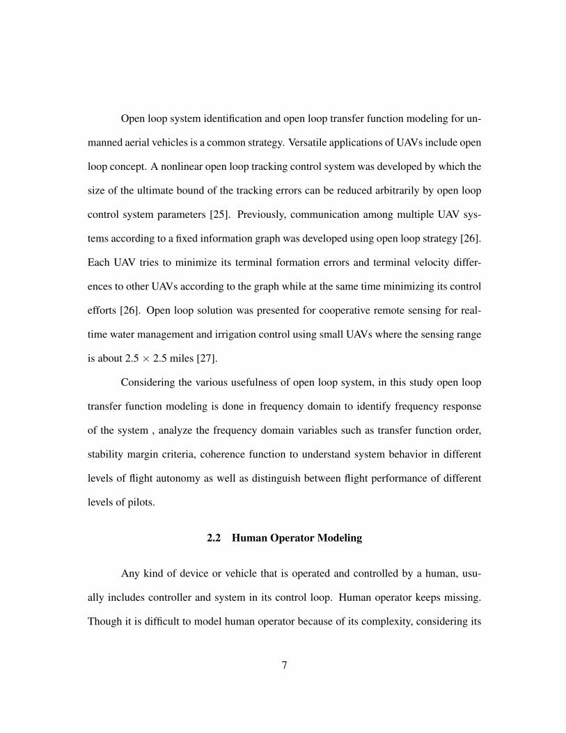
Considering the various usefulness of open loop system, in this study open loop
transfer function modeling is done in frequency domain to identify frequency response
of the system , analyze the frequency domain variables such as transfer function order,
stability margin criteria, coherence function to understand system behavior in different
levels of flight autonomy as well as distinguish between flight performance of different
levels of pilots.
2.2 Human Operator Modeling
Any kind of device or vehicle that is operated and controlled by a human, usu-
ally includes controller and system in its control loop. Human operator keeps missing.
Though it is difficult to model human operator because of its complexity, considering its
7
significance, research were done before to model human operator. A method was devel-
oped for modeling the human operator from actual input-output data utilizing time series
analysis [28]. The technique first identified the form of the model and then estimated the
parameters of the identified model based on actual data. The model helps to compensatory
tracking data and has the potential for model building of any data that is corrupted with
noise. Time series analysis was also applied to model human operator dynamics in pursuit
and compensatory tracking modes by a second order dynamic system that shows human
operator is not a generator of periodic characteristics [29]. Factors related to human op-
erator are very important in system identifications for manned aerial vehicles, unmanned
aerial vehicles, military aircrafts and so on [28]. Human operator model was developed
for UAV search scheduling to include human-in-the-loop for scheduling, replanning task
for a simulated UAV mission [30]. Comparisons were made between the expected perfor-
mance difference between the scheduling system and a greedy scheduling strategy rep-
resentative of operator planning, showing the potential for improvement of the proposed
strategy [30]. This design maximizes the operator’s accumulated reward of the search
tasks in a time-pressured environment [30]. Individual task specific workload dependent
human behaviour patterns were observed and from the patterns task situations, operator
performance and human error during task processing were derived that shows the devel-
opment of a knowledge based cognitive, cooperative assistance system for multi-UAV
guidance [31]. Pilot modeling was also performed to develop predictive models to deter-
mine operator capacity for controlling multiple UAVs [32]. Effects of increasing number
of UAVs and/or system autonomy can be seen on system performance as well as operator
8

performance that helps to predict operator capacity [32].
As pilots have significant role while flying the unmanned aircraft to deal with the
complexity and unpredictability of real-world scenarios and human operators’ presence
is also crucial for taking the responsibility of critical decisions in high risk situations, in
this study, human operator is introduced as a pilot transfer function and included with
controller and UAV transfer function to generate the combined pilot (P), controller (C)
and UAV (U) open loop transfer function.
2.3 Transfer Function Modeling
The transfer function of a system is the relationship of the system’s output to its
input, represented in the complex Laplace domain [24]. Time and frequency domain anal-
ysis are done widely in transfer function modeling. In case of unmanned aerial vehicles,
transfer function modeling in frequency domain has become popular as system complex-
ity, stability and control derivatives can be efficiently derived from frequency response
of the system [33]. Time domain flight data collection and analysis is also important
as frequency domain system identification relies on the conversion of time domain fight
data into the frequency domain [33]. Transfer function modeling in frequency domain
has been applied for UAVs of different scales such as multi rotor UAV [34], fixed-wing
UAV [33], helicopter [35, 36, 37, 38]. Transfer function modeling was performed for fre-
quency response identification of the unamnned aircraft system [33]. A dynamic model
was derived from transfer function modeling (in both frequency and time domain) for
9
both hover and cruise flight conditions and the accuracy of the developed model was ver-
ified by the comparison between predicted and actual responses from the model and the
flight experiments [35]. Transfer function modeling for hovering and guidance control
for autonomous small-scale unmanned helicopter was utilized to reduce the overshoot of
the system [39]. For unmanned aircraft systems, transfer function modeling in frequency
domain was helpful to model both angular positions [37] and rates [38].
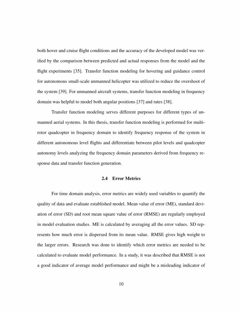
Transfer function modeling serves different purposes for different types of un-
manned aerial systems. In this thesis, transfer function modeling is performed for multi-
rotor quadcopter in frequency domain to identify frequency response of the system in
different autonomous level flights and differentiate between pilot levels and quadcopter
autonomy levels analyzing the frequency domain parameters derived from frequency re-
sponse data and transfer function generation.
2.4 Error Metrics
For time domain analysis, error metrics are widely used variables to quantify the
quality of data and evaluate established model. Mean value of error (ME), standard devi-
ation of error (SD) and root mean square value of error (RMSE) are regularly employed
in model evaluation studies. ME is calculated by averaging all the error values. SD rep-
resents how much error is dispersed from its mean value. RMSE gives high weight to
the larger errors. Research was done to identify which error metrics are needed to be
calculated to evaluate model performance. In a study, it was described that RMSE is not
a good indicator of average model performance and might be a misleading indicator of
10
average error, and thus ME would be a better metric for that purpose [12]. Later it was
shown that the avoidance of RMSE in favor of ME is not the solution [40]. In fact, the
RMSE is more appropriate to represent model performance than the ME when the error
distribution is expected to be Gaussian [40]. However, RMSE is superior over the ME
cannot be contended. Instead, a combination of metrics, including but certainly not lim-
ited to RMSEs and MEs, are often required to assess model performance. Another error
metric that is used frequently to evaluate errors is standard deviation (SD). The main ex-
ception of standard deviation is when the measurement error depends on the size of the
measurement, usually with measurements becoming more variable as the magnitude of
the measurement increases [13].
Considering usefulness of all the error metrics, to quantify pilot and UAV per-
formance in time domain, mean value of path error, standard deviation of path error and
root mean square value of path error is calculated. ME gives an estimation of average
performance of both pilot and quadcopter. SD is calculated to identify the probability of
making errors by different pilots in different flight autonomy modes while following the
path. RMSE is estimated to quantify pilot and quadcopter performance based on larger
errors made by pilots during flight testing.
2.5 Stability Margin Criteria
Stability of a system in open loop is quantified by two margin values, gain and
phase margin. The phase margin measures how much phase variation is needed at the gain
crossover frequency to lose stability. Similarly, the gain margin measures what relative
11

gain variation is needed at the phase crossover frequency to lose stability [24]. The gain
crossover frequency is the frequency where the amplittude ratio of input and output of
a system is 1, or when magnitude is equal to 0 dB. The phase crossover frequency is
the frequency where phase shift between input and output of a system is equal to -180
degrees. Together, these two numbers give an estimate of the safety margin for open-loop
stability [24]. Gain and phase margin can be interpreted from Figure 2.
Figure 2: Interpretation of gain and phase margin from bode plot
From Figure 2, the gain is 0 dB at 0.25 rad/s. Gain crossover frequency is 0.25
rad/s and at this frequency phase margin is -51.3 deg. The phase difference between input
and output is -180 deg at 0.217 rad/s and at this frequency gain margin is -84.7 dB. Gain
value of 0 dB and phase value of -180 deg are avoided to ensure stability of a system.
For this reason, the gain and phase margin values at the crossover frequencies denotes
stability of the system. Higher margin values indicates more stability of a system in open
12
loop. The smaller the stability margins, the more fragile the system is [41].
Research on stability margin analysis is done for safety purposes. A method was
proposed to obtain complete information about the effects of adjustable parameters on
gain and phase margins to a pitch rate control system [42]. This control system was ap-
plied for a re-entry vehicle and comparisons with results of previous work are made suc-
cessfully [42]. The change in gain and phase margins for dynamic compensation control
of a rotary wing UAV using positive position feedback was analyzed to design the feed-
back controller [43]. The controller takes advantage of the two level hierarchical control
schemes without penalizing the phase response and mitigates the presence of flybar [43].
An autopilot design of tilt-rotor UAV using particle swarm optimization method consid-
ered stability margin criteria to evaluate the control system for stability and the designed
control guarantees the satisfaction of the control system requirement ensuring a sufficient
stability margin of the control system in both helicopter and airplane mode [44]. For
dynamic modeling and stabilization techniques for tri-rotor UAV, stability margins were
used to check stability of the system and the altitude and attitude channels show infinity
gain margin representing stable behavior of the system [45].
To analyze the stability of UAV in open loop, stability margin is a widely used
criteria. In this study, stability gain and phase margin criteria on the frequency domain
transfer function model is analyzed for each pilot’s flight test in each autonomy level.
Gain and phase margin values differ with respect to different levels of pilots as well as
different levels of flight autonomy. The stability margin value is considered as a predictor
in the regression modeling to predict both pilot and UAV levels.
13
2.6 Cooper-Harper Rating Scale
In 1969, George E. Cooper and Robert P. Harper Jr. established a rating scale
for pilots to give rating to the aircraft for handling quality specifications to identify how
efficient the aircraft is to accomplish a task [46]. New definition of handling qualities
was proposed which emphasizes the importance of factors that influence the selection
of a rating other than stability and control characteristics. The experimental use of pilot
rating is discussed in detail, with special attention devoted to clarifying the difference
between mission and task, identifying what the rating applies to and considering the pilot’s
assessment criteria [46].
Later M. Christopher Cotting modified the C-H (Cooper-Harper) scale to use for
performance evaluation of unmanned aerial vehicle. This modified scale not only evalu-
ates the unmanned aerial vehicle in flight but also takes into account sensor package and
successfully evaluates the integrated system’s mission effectiveness [1]. Figure 3 shows
the modified Cooper-Harper rating scale for unmanned aircraft.
Modified C-H scale was also used for performance evaluation in UAV displays.
The Modified Cooper Harper for Unmanned Vehicles Displays (MCH-UVD), modifies
the commonly used Cooper-Harper manned aircraft assessment tool by shifting empha-
sis away from evaluating the physical control of an aircraft, to evaluating how well the
displays support basic operator information processing [47].It helps to identify what level
of information processing and decision support the interface provides to UAV operators
- activities critical to the success of most UAV missions [47]. Modified Cooper-Harper
rating scale was abbreviated and used for handling quality specifications and rate mission
14

effectiveness for Vertical Take-Off and Landing (VTOL) UAV [20].
As Cooper-Harper rating scale reflects pilots’ opinion about the UAV system per-
formance, this rating is a useful tool to identify how the performance of the same quad-
copter system varies with respect to different levels of pilots. After completing the path
following task, each pilot is introduced to the abbreviated modified C-H scale for UAV
and pilots’ given rating in a scale of 1-10 is used as a predictor in the modeling to quantify
pilot and quadcopter performance individually.
2.7 Logistic Regression Modeling
When the dependent variable consists of two categories that are not ordinal (no
natural ordering), the ordinary least square estimator cannot be used. Instead, a maximum
likelihood estimator like binary logistic regression (BLR) technique is used. Multinomial
logistic regression (MLR) is an extension of binary logistic regression (BLR). MLR is
used when dependent variable consists of more than two categories. Logistic regression
has versatile applications such as research in the application of nursing [23], bioinformat-
ics [48], drones [49] and so on.
Binary logistic regression was used to create models to predict factors of failure
in operating UAV with two possible outcomes, operator failure and mechanical failure
in the U.S. Air Force and the outcome was operator failure caused more than half of the
mishaps [50]. In case of unmanned aerial vehicle, for multilabeling UAV imagery, typi-
cally characterized by a high level of information content, multinomial logistic regression
technique was used [51]. Experiments conducted on two different UAV image data sets
15
demonstrate the promising capability of the proposed method done by multinomial lo-
gistic regression modeling [51]. In a study multinomial logistic regression modeling was
used to explain opposition to US drone strikes in Pakistan [52]. The model tests hypothe-
ses related to respondents attitudes toward the US drone attack where support coded 1,
opposition coded -1 and do not know or no response coded 0 [52]. This study helps to
understand the shape of attitudes in Pakistan toward American drone strikes.
In this study, regression model outcome, pilot level has two categories and UAV
autonomy level has three categories. For this reason, to predict pilot level, BLR and to
predict UAV autonomy level, MLR is used and time and frequency domain variables and
C-H rating scale is used as predictors in the modeling. The regression equations and
modeling steps are described in the methodology section.
16
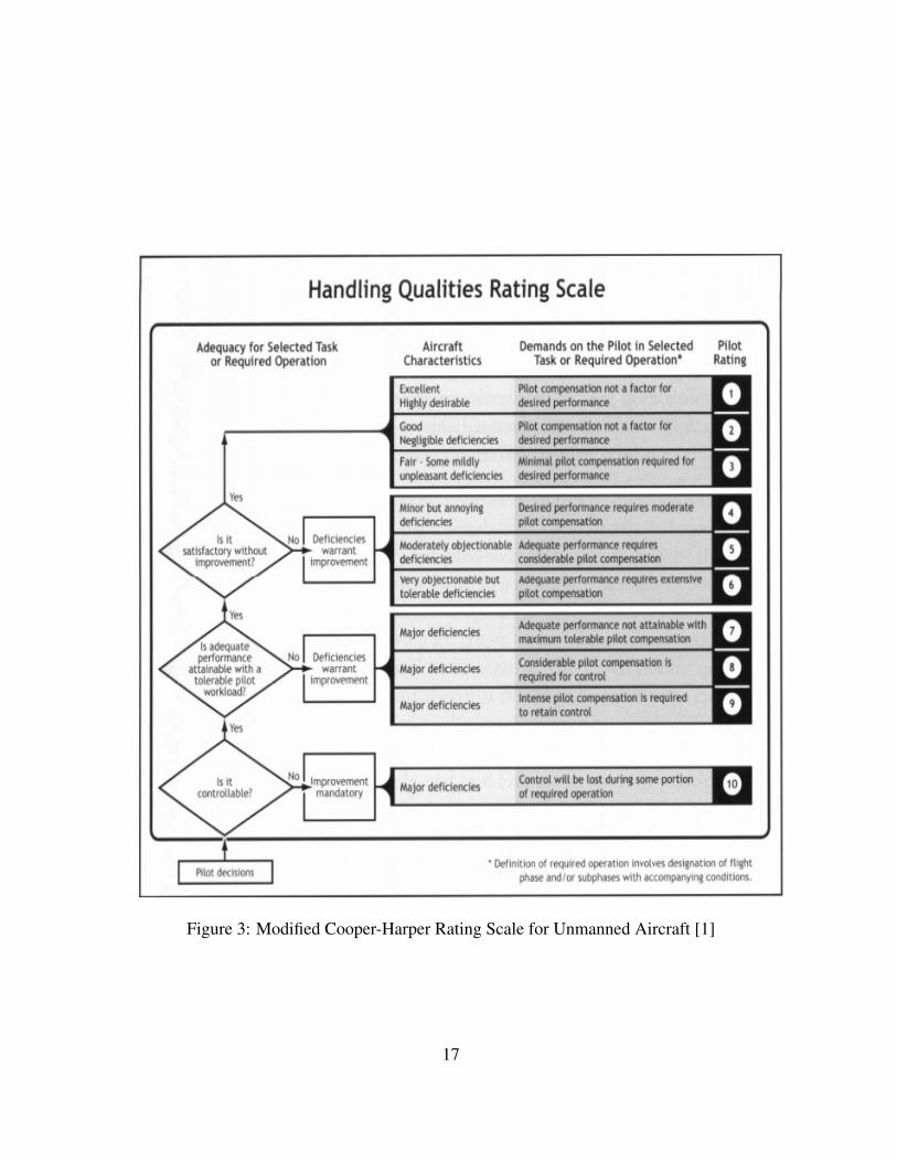
Figure 3: Modified Cooper-Harper Rating Scale for Unmanned Aircraft [1]
17
CHAPTER 3
METHODOLOGY
This chapter discusses the experiments conducted and flight data analysis tech-
niques used for evaluating pilot and quadcopter performance based on a mission task of
following a desired path. The modeling technique that is developed to quantify pilot and
quadcopter performance helps to classify pilot experience level and level of autonomy
of unmanned aircraft into specific categories by analyzing the flight test results. At the
beginning, the selection process of pilots with different experience levels and unmanned
aircraft with different autonomy levels is discussed. Then an overview of the unmanned
system configuration and path planning technique across the test arena is included. Next,
transfer function modeling, time and frequency domain analysis and Cooper-Harper rat-
ing scale are explained elaborately to quantify pilot and quadcopter performance. In the
end, flight variable dependency test, modeling of pilot experience level and quadcopter
autonomy levels and a test case to verify the established model are discussed.
3.1 Test Arena & Path Planning
The schematic diagram of the desired path is shown in Figure 4. The mission task
is to fly the unmanned aircraft through the gates and follow the desired path according to
the arrow marks shown. The first marker is set as a starting point where the pilot takes off
and lands the quadcopter. The second marker is set at the farthest point of the path where
18

the pilot makes the turn to complete the path. The desired path is generated by walking
through a pre-specified path, holding the quadcopter that has a GPS antenna mounted on
it. The GPS antenna gives longitude (degree) and latitude (degree) data, that are used to
quantify the desired path. Longitude (degree) and latitude (degree) data is converted to X
axis and Y axis displacement (ft) and used as coordinates to show distance along the path
and calculate path errors.
Figure 4: Schematic diagram of desired path
The flight testing is conducted at an outdoor area (Figure 5) of University of
Missouri-Kansas City (UMKC). Four steel rods are used to make two gates (Figure 6)
and two steel rods are used as two markers in the flight path (Figure 7). Two gates are set
up on two sides of the tracking path.
19
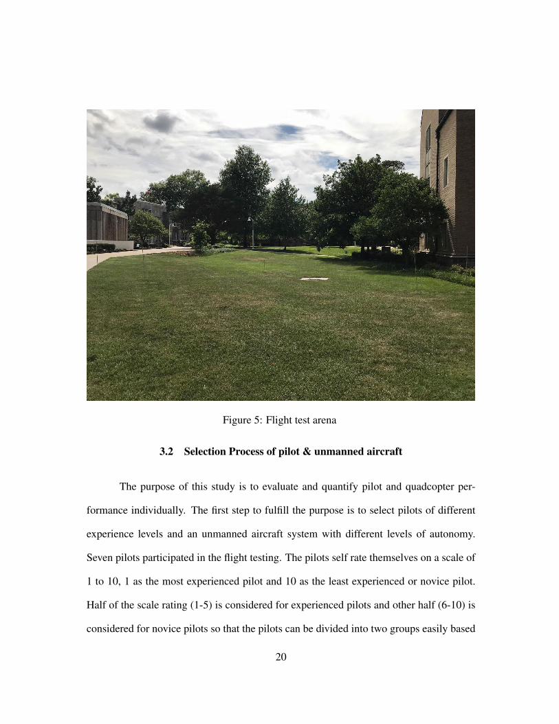
Figure 5: Flight test arena
3.2 Selection Process of pilot & unmanned aircraft
The purpose of this study is to evaluate and quantify pilot and quadcopter per-
formance individually. The first step to fulfill the purpose is to select pilots of different
experience levels and an unmanned aircraft system with different levels of autonomy.
Seven pilots participated in the flight testing. The pilots self rate themselves on a scale of
1 to 10, 1 as the most experienced pilot and 10 as the least experienced or novice pilot.
Half of the scale rating (1-5) is considered for experienced pilots and other half (6-10) is
considered for novice pilots so that the pilots can be divided into two groups easily based
20

Figure 6: Steel rod gates through which the quadcopter is flown by pilots to follow thedesired path
on the rating scale. According to the self rating, three pilots are placed in the experienced
category and other four are placed in the novice category. Self rating of pilots are used to
divide them into two groups. Table 1 shows self rating of pilots and their corresponding
category based on experience levels.
Table 1: Pilot self rating & experience levelPilot Self Rating Category
Pilot 1 1 ExperiencedPilot 2 2 ExperiencedPilot 3 2 ExperiencedPilot 4 7 NovicePilot 5 7 NovicePilot 6 8 NovicePilot 7 8 Novice
The level of autonomy of the unmanned aircraft denotes how autonomous the
unmanned system is and the ease of control a pilot has when the quadcopter is flown.
For the tested quadcopter, Level 1 autonomy is the linear position tracking mode or GPS
mode. In this autonomy level, the unmanned aircraft receives GPS data (x,y,z) to hold
21
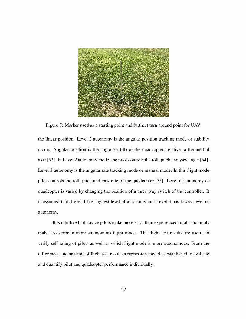
Figure 7: Marker used as a starting point and furthest turn around point for UAV
the linear position. Level 2 autonomy is the angular position tracking mode or stability
mode. Angular position is the angle (or tilt) of the quadcopter, relative to the inertial
axis [53]. In Level 2 autonomy mode, the pilot controls the roll, pitch and yaw angle [54].
Level 3 autonomy is the angular rate tracking mode or manual mode. In this flight mode
pilot controls the roll, pitch and yaw rate of the quadcopter [55]. Level of autonomy of
quadcopter is varied by changing the position of a three way switch of the controller. It
is assumed that, Level 1 has highest level of autonomy and Level 3 has lowest level of
autonomy.
It is intuitive that novice pilots make more error than experienced pilots and pilots
make less error in more autonomous flight mode. The flight test results are useful to
verify self rating of pilots as well as which flight mode is more autonomous. From the
differences and analysis of flight test results a regression model is established to evaluate
and quantify pilot and quadcopter performance individually.
22
3.3 System Configuration
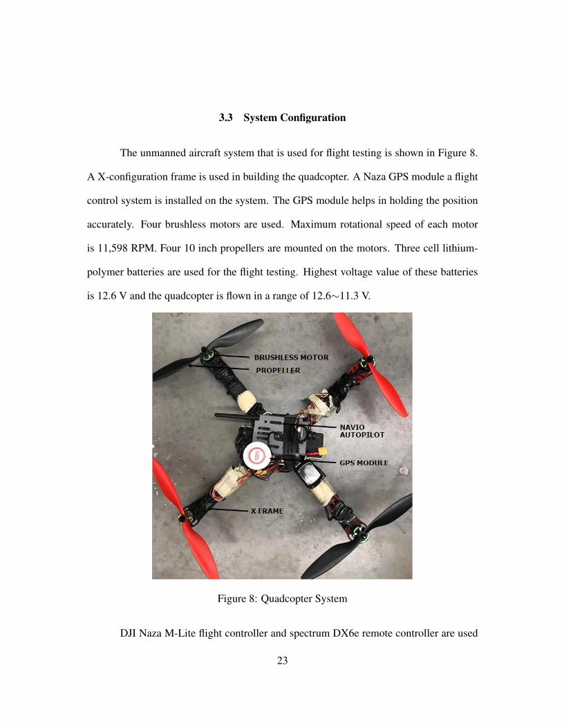
The unmanned aircraft system that is used for flight testing is shown in Figure 8.
A X-configuration frame is used in building the quadcopter. A Naza GPS module a flight
control system is installed on the system. The GPS module helps in holding the position
accurately. Four brushless motors are used. Maximum rotational speed of each motor
is 11,598 RPM. Four 10 inch propellers are mounted on the motors. Three cell lithium-
polymer batteries are used for the flight testing. Highest voltage value of these batteries
is 12.6 V and the quadcopter is flown in a range of 12.6∼11.3 V.
Figure 8: Quadcopter System
DJI Naza M-Lite flight controller and spectrum DX6e remote controller are used
23

for flight testing. Table 2 shows the specifications of the flight controller. The Naza M-
Lite flight controller is configured using the Naza lite independent assistant software and
firmware. The software is used to assign switches of the remote controller to specific
range of values so that by switching the values, desired functionality of the flight con-
troller can be achieved. Software changes needed to support variation of the autonomy
level of unmanned aircraft and command limit are facilitated by the modular architecture
of the fight controller which is based on the specific model of the flight controller.
Table 2: Specifications of flight controller
Parameters Values
Refresh Frequency 400 Hz
Voltage Range 7.2V ∼ 26.0 V(2S ∼ 6S LiPo)
Power 0.6W (0.12A @ 5V)
Hovering Accuracy Vertical:± 0.8m, Horizontal:± 2.5m
Max Tilt Angle 45 degrees
Built-In Function Three Modes Autopilot
Raspberry Pi 3 and Navio 2 autopilot are used as a data logger to log all the neces-
sary flight information for further analysis. Flight information such as remote controller
(RC) commands, GPS longitude and latitude information, sampling time, intertial mea-
surement units (IMU) sensor information such as angular positions, angular rates etc. are
logged. The Navio2 provides sensor information from dual 9 degree-of-freedom (DOF)
intertial measurement units (IMU) to the RaspberryPi 3. The sampling frequency is 100
Hz and the attitude estimate is provided by a Madgwick Filter [56] algorithm operating
at 300 Hz. To facilitate the efficient collection of experimental data, the system can be
24

activated remotely via radio control (RC) transmitter so that a remote operator can start
and stop multiple experimental trials without interacting with a computer.
3.4 Time Domain Analysis
Errors made by the pilots while following the path with respect to time is used
for time domain analysis to quantify pilot and quadcopter performance. The following
subsections discuss the techniques used to calculate path error and error metrics for time
domain analysis.
3.4.1 Path Error
To calculate the path error, the GPS longitude and latitude data is converted to
feet from degrees and named as X axis displacement and Y axis displacement, respec-
tively. The path error at a specific point is calculated from the resultant of X axis error
Equation (3.1) and Y axis error Equation (3.2). The equation Equation (3.3) shows the
resultant path error, E.
∆X = Xdesired −Xactual (3.1)
∆Y = Ydesired − Yactual (3.2)
E =√
(∆X)2 + (∆Y )2 (3.3)
The path error made by the pilots are quantified by calculating three error metrics,
25

mean value of path error (ME), standard deviation of path error (SD) and root mean square
of path error (RMSE). The equations for these error metrics calculation are shown in the
following sections.
3.4.2 Mean Value of Path Error (ME)
In the calculation of mean value of path error, all the errors made by a pilot through
the whole path are averaged. Equation (3.4) are used to calculate the mean value of path
error where N is the total number points along the whole path.
Emean =ΣNi=1∆EiN
(3.4)
The mean value of path error actually gives a holistic idea of the flight test, how
closely the pilot follows the path. But if a pilot makes a bigger error at a specific point and
comes back to track to the next point while flying, mean value of error does not specify
that error for that particular point. Standard deviation of error (SD) and root mean square
value of error (RMSE) are two very useful metrics to identify the deviation of error from
mean or desired value and comparatively larger errors respectively.
3.4.3 Standard Deviation of Path Error (SD)
Standard deviation of error (SD) shows how much error is dispersed from its
mean [13]. A low SD indicates that the data points tend to be close to the mean or desired
value of the set, while a high standard deviation indicates that the data points are spread
out over a wider range of values. Equation (3.5) is used for the calculation of standard
deviation of error.
26
σ =
√ΣNi=1(Ei − Emean)2
N − 1(3.5)
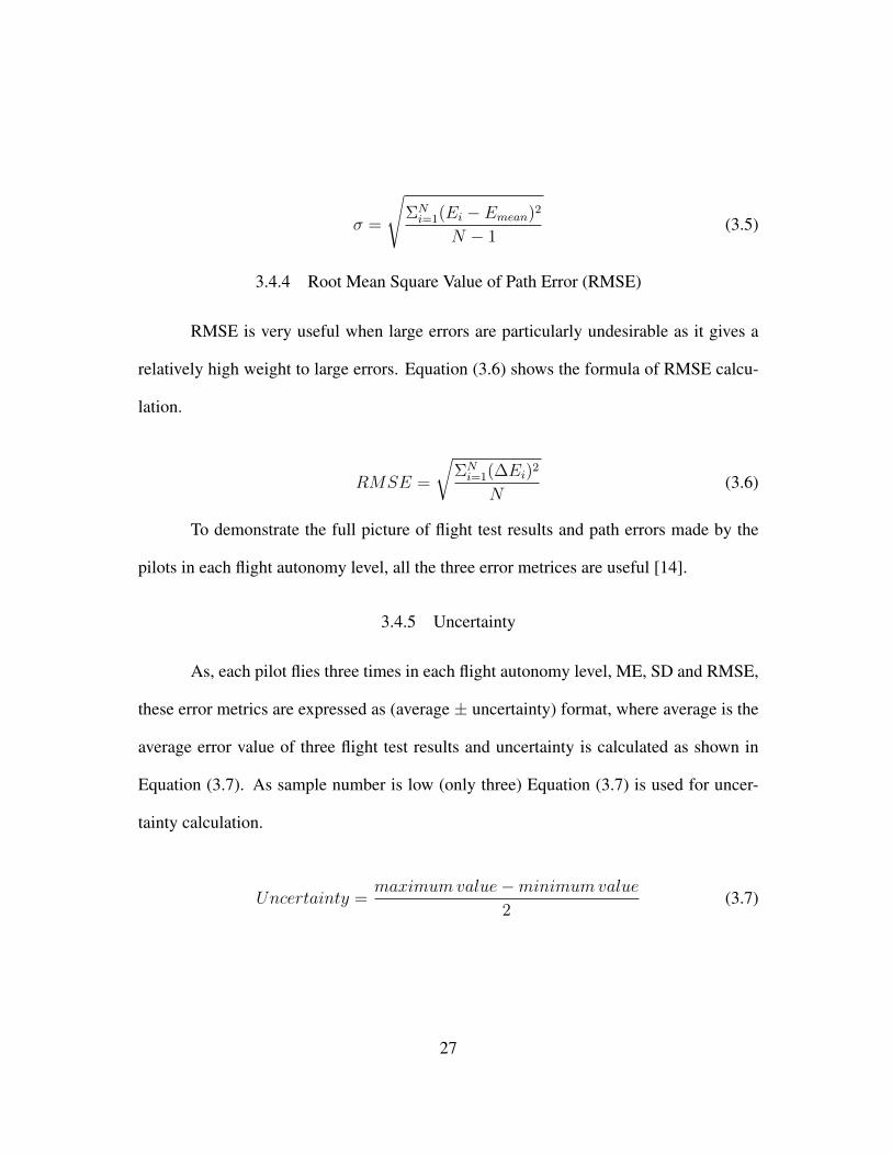
3.4.4 Root Mean Square Value of Path Error (RMSE)
RMSE is very useful when large errors are particularly undesirable as it gives a
relatively high weight to large errors. Equation (3.6) shows the formula of RMSE calcu-
lation.
RMSE =
√ΣNi=1(∆Ei)
2
N(3.6)
To demonstrate the full picture of flight test results and path errors made by the
pilots in each flight autonomy level, all the three error metrices are useful [14].
3.4.5 Uncertainty
As, each pilot flies three times in each flight autonomy level, ME, SD and RMSE,
these error metrics are expressed as (average ± uncertainty) format, where average is the
average error value of three flight test results and uncertainty is calculated as shown in
Equation (3.7). As sample number is low (only three) Equation (3.7) is used for uncer-
tainty calculation.
Uncertainty =maximumvalue−minimumvalue
2(3.7)
27

3.5 Frequency Domain Analysis
Transfer function modeling in frequency domain is done to analyze frequency
response of the system. From the MIMO (Multi Input Multi Output) transfer function
modeling, frequency domain variables such as transfer function order [24], reliable fre-
quency [18], coherence function value [18], stability margin criteria [19] are acquired to
quantify pilot and quadcopter performance based on frequency response of the system.
3.5.1 Transfer Function Modeling
Previously, transfer function modeling for unmanned aircraft systems included a
combination of controller and UAV transfer functions [16]. Pilot transfer function keeps
missing from the system transfer functions. In this study, the transfer function is generated
in frequency domain by combining pilot, controller and UAV transfer functions. For
Controller(C) and UAV(U) transfer function, controller stick command (linear or angular
positions or rates) is the input and longitude (Xa) and latitude (Ya) coordinate values of
actual path are considered as the output and it is a SIMO (Single Input Multi Output)
transfer function shown in Figure 9. For the pilot transfer function, longitude (Xd) and
latitude (Yd) coordinate values of desired path are considered as input and controller stick
command is considered as output and it is a MISO (Multi Input Single Output) transfer
function as shown in Figure 10.
Figure 9: Controller and UAV transfer function combined together
28
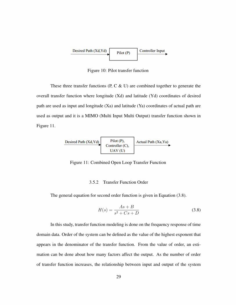
Figure 10: Pilot transfer function
These three transfer functions (P, C & U) are combined together to generate the
overall transfer function where longitude (Xd) and latitude (Yd) coordinates of desired
path are used as input and longitude (Xa) and latitude (Ya) coordinates of actual path are
used as output and it is a MIMO (Multi Input Multi Output) transfer function shown in
Figure 11.
Figure 11: Combined Open Loop Transfer Function
3.5.2 Transfer Function Order
The general equation for second order function is given in Equation (3.8).
H(s) =As+B
s2 + Cs+D(3.8)
In this study, transfer function modeling is done on the frequency response of time
domain data. Order of the system can be defined as the value of the highest exponent that
appears in the denominator of the transfer function. From the value of order, an esti-
mation can be done about how many factors affect the output. As the number of order
of transfer function increases, the relationship between input and output of the system
29

becomes complicated or the system exhibits a wider range of responses that must be ana-
lyzed and described [24]. Transfer function order is estimated to identify the complexity
of input-output relationship of the system.
3.5.3 Reliable Frequency & Coherence Function
To demonstrate the frequency response of a system, bode plots and coherence
function plots are useful. Bode plots contain magnitude and phase curves from where the
reliable frequency range to correctly express input-output relationship of the system can
be identified. Magnitude and phase curves remain stable upto a specific frequency. The
frequency is known as the reliable frequency [18]. After the reliable frequency, input-
output relationship is not reliable as the magnitude and phase curves begin to oscillate
dramatically [18]. With the bode plot, coherence function is plotted with respect to fre-
quency, shown in results and discussions section. The coherence function value is used
to assess the accuracy of the frequency response identification. Coherence value ranges
from 0 to 1. The frequency range where coherence function value is > 0.6 and coherence
function curve is not oscillating, is considered that the frequency response has accpetable
accuracy in that range. A rapid drop or oscillation in the coherence function for a par-
ticular range of frequencies indicates poor frequency-response identification accuracy in
that region [18]. The reliable frequency gives an approximate estimation and coherence
function values give the actual frequency range where the input-output relationship of the
system is accurate [18].
30

3.5.4 Stability Margin Criteria
The stability margin criteria includes two values, gain margin (Gm) and phase
margin (Pm). These two values are estimated to find out the safety margin of open loop
stability of the system. System stability is proportional to the safety margin values. The
smaller value of safety margins indicate a fragile system, whereas a larger value indicates
more stable system. Gain and phase margins are estimated in frequency domain to identify
the system stability in different levels of flight autonomy and differentiate between flight
perfromance of different levels of pilots [24].
3.6 Cooper-Harper Rating Scale
Apart from time and frequency domain analysis, an unmanned aircraft rating given
by the pilots is used for evaluating pilot and quadcopter performance. The abbreviated
version of the modified Cooper-Harper rating scale is used by the pilots to rate the air-
craft that governs the ease and precision with which the pilot can accomplish a task in
support of an aircraft. The modified version [1] of the Cooper-Harper scale is abbrevi-
ated [20] so that the rating scale can be shortened from 10 to 4 levels and becomes easier
for pilots to rate the unmanned aircraft system quickly. Immediately after completing
the pre-specified task of following the desired path, pilots are given the rating scale to
evaluate the aircraft. This rating represents the opinion of pilots about the quadcopter’s
performance in different levels of autonomy.
Table 3 shows abbreviated modified Cooper-Harper Rating scale for UAV tasks.
Pilot rating of Level 1 indicates C-H rating range of 1-3. Pilots in this category rate the
31
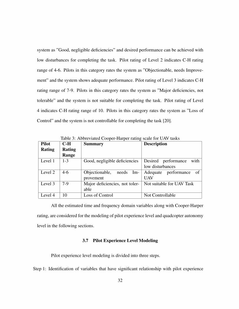
system as ”Good, negligible deficiencies” and desired performance can be achieved with
low disturbances for completing the task. Pilot rating of Level 2 indicates C-H rating
range of 4-6. Pilots in this category rates the system as ”Objectionable, needs Improve-
ment” and the system shows adequate performance. Pilot rating of Level 3 indicates C-H
rating range of 7-9. Pilots in this category rates the system as ”Major deficiencies, not
tolerable” and the system is not suitable for completing the task. Pilot rating of Level
4 indicates C-H rating range of 10. Pilots in this category rates the system as ”Loss of
Control” and the system is not controllable for completing the task [20].
Table 3: Abbreviated Cooper-Harper rating scale for UAV tasksPilotRating
C-HRatingRange
Summary Description
Level 1 1-3 Good, negligible deficiencies Desired performance withlow disturbances
Level 2 4-6 Objectionable, needs Im-provement
Adequate performance ofUAV
Level 3 7-9 Major deficiencies, not toler-able
Not suitable for UAV Task
Level 4 10 Loss of Control Not Controllable
All the estimated time and frequency domain variables along with Cooper-Harper
rating, are considered for the modeling of pilot experience level and quadcopter autonomy
level in the following sections.
3.7 Pilot Experience Level Modeling
Pilot experience level modeling is divided into three steps.
Step 1: Identification of variables that have significant relationship with pilot experience
32

level and can be used as independent variables in the modeling to predict pilot
level.
Step 2: Pilot experience level modeling using binary logistic regression technique to show
how the increase and decrease in the value of independent variables changes the
outcome of the model.
Step 3: Conducting a single flight test with an eighth pilot, analyzing flight variables from
flight data and using as independent variables in the established model equation to
verify if the model can predict the pilot experience level correctly.
3.7.1 Independent Sample t Test
The independent sample t test compares the means of two independent groups
in order to determine whether there is statistical evidence that the associated population
means are significantly different. The independent variable needs to be categorical. To
find out the difference between two independent groups null hypothesis (H0) and alter-
native hypothesis (H1) are set. The null hypothesis (H0) and alternative hypothesis (H1)
of the independent sample t test can be expressed by Equation (3.9) and Equation (3.10)
respectively.
H0 : µ1 = µ2 (the two populationmeans are equal) (3.9)
H1 : µ1 6= µ2 (the two populationmeans are not equal) (3.10)
33
Here µ1 and µ2 are the population means for group 1 and group 2, respectively. To
accept or reject a hypothesis, a significance value (P value) [57] is calculated using Inde-
pendent Sample t Test. If P value < 0.05, there is a significant difference between the two
population means and null hypothesis is rejected. If P value≥ 0.05, there is no significant
difference between two population means and alternate hypothesis is rejected [21]. The
significance value (P value) estimation of 0.05 comes from the 95% confidence interval
criteria. A 95% confidence interval is a range of values that gives 95% certainty that the
samples contain the true mean of the population.
In this study, pilot experience level has two categories. For independent sample t
test, pilot experience level is considered as an independent variable and dependent vari-
ables included all the time and frequency domain variables along with Cooper-Harper
rating scale. The variables that yield P values < 0.05, are included in the modeling of
pilot experience level. The variables that show P value ≥ 0.05, do not have a significant
relation with the pilot experience level and are not included in the modeling.
3.7.2 Binary Logistic Regression
Time domain variables (error metrics), frequency domain variables (transfer func-
tion order, coherence function and gain margin) and Cooper-Harper rating scale are con-
sidered as independent variables to model the dependent variable, (pilot experience level)
using binary logistic regression. The dependent variable is divided into two groups la-
beled ‘0’ and ‘1’, where ‘0’ is the comparison group and ‘1’ is the referent group. For
pilot experience level, experienced pilots are considered as comparison group and novice
34
pilots as referent group. As a linear predictor function, binary logistic regression equation
can be written as Equation (3.11).
f(i) = β0 + β1.x1,i + ...+ βm.xm,i (3.11)
where β0, β1,..., βm are regression coefficients indicating the relative effect of a
particular independent variable on the outcome. The regression coefficients are grouped
into a single vector β of size m + 1. For each observation i, an additional explanatory
pseudo-variable x0,i is added, with a fixed value of 1, corresponding to the intercept co-
efficient β0. The resulting explanatory variables x0,i, x1,i, ..., xm,i are then grouped into a
single vector Xi of size m+ 1.
The compact form of binary logistic regression equation can be written as Equa-
tion (3.12).
f(i) = β.Xi (3.12)
Here β is the set of regression coefficients are grouped into a single vector of
size m + 1. and Xi is the set of explanatory variables associated with observation i.
Exponential of coefficients, Exp(β) are known as odds ratio. Odds ratio is calculated
to find out how the increase or decrease in an independent variable or predictor’s value
changes the outcome of the model. An odds ratio> 1 indicates that the risk of the outcome
falling in the comparison group relative to the risk of the outcome falling in the referent
group increases as the variable increases. In other words, the comparison group outcome
is more likely. An odds ratio < 1 indicates that the risk of the outcome falling in the
35
comparison group relative to the risk of the outcome falling in the referent group decreases
as the variable increases, the referent group is more likely [22].
3.7.3 Verification Test Case
In the end, a test case is included to verify the model where an eighth pilot is
assigned to do the same task with the same quadcopter. The Level of autonomy of UAV is
kept unknown to the pilot and both the pilot level and autonomy level of unmanned aircraft
is predicted by analyzing the flight test data and using the model. Time and frequency
domain analysis are done on the collected flight test data. The pilot is also introduced
with the Cooper-Harper rating scale to rate the unmanned aircraft system. After getting
all the explanatory variables or predictors Xi, they are used on the right hand side of
Equation (4.1) to estimate the probability of predicting experienced or novice pilot, based
on the explanatory variables.
P (experienced) =eβ1.x1+...+βm.xm
1 + eβ1.x1+...+βm.xm(3.13)
Left hand side of Equation (4.1) estimates the probability of pilot being experi-
enced, as the coefficients, β on the ride hand side are acquired from comparison group
(experienced) of binary logistic regression. Based on the value of probability of Equa-
tion (4.1), the pilot experience level can be predicted.
3.8 Autonomy Level of UAV Modeling
The autonomy level of UAV modeling is also divided into three steps.
36
Step 1: Identification of variables that have significant relationship with autonomy level of
unmanned aircraft and can be used as independent variables in the modeling to
predict flight autonomy level.
Step 2: Level of autonomy of aircraft modeling using multinomial logistic regression tech-
nique to show how the increase and decrease in the value of independent variables
changes the outcome of the model.
Step 3: Conducting a single flight test with an eighth pilot, analyzing flight variables from
flight data and using as independent variables in the established model equation to
verify if the model can predict the flight autonomy level correctly.
3.8.1 ANOVA Test
One way ANOVA is an extension of independent sample t test. Independent sam-
ple t test is used to differentiate between two independent groups. The same concept of
hypothesis testing and significance value are used for ANOVA test, the difference is that
ANOVA generalizes the t test to more than two groups. As, level of autonomy has three
categories, ANOVA test is done to find out which variables have an overall effect on the
flight autonomy levels. The significant relationship among variables can be identified
from P values, same as t test. After the one way ANOVA test, a post hoc test using Tukey
method [58] is performed to identify which flight autonomy levels are different from each
other among the three and where the difference lies.
37
3.9 Multinomial Logistic Regression
Time domain variables (error metrics), frequency domain variables (transfer func-
tion order, coherence function and gain margin) and Cooper-Harper rating scale are con-
sidered as independent variables to model the dependent variable (level of autonomy of
unmanned aircraft) using multinomial logistic regression (MLR). Multinomial logistic re-
gression uses a linear predictor function f(k, i) to predict the probability that observation
i has on outcome k Equation (3.14).
f(k, i) = β0,k + β1,k.x1,i + ...+ βm,k.xm,i (3.14)
where βm,k is a regression coefficient associated with themth explanatory variable
and the kth outcome. As explained in the binary logistic regression section, the regression
coefficients and explanatory variables are normally grouped into vectors of size m+ 1, so
that the predictor function can be written more compactly as Equation (3.14)
f(k, i) = βk.Xi (3.15)
Here βk is the set of regression coefficients associated with outcome k, and Xi is
the set of explanatory variables associated with observation i. Exponential of coefficients,
Exp(βk) are known as odds ratio. Odds ratio is calculated to find out how the increase
or decrease in an independent variable or predictor’s value changes the outcome of the
model. An odds ratio > 1 indicates that the risk of the outcome falling in the comparison
group relative to the risk of the outcome falling in the referent group increases as the
38

variable increases. In other words, the comparison group outcome is more likely. An
odds ratio < 1 indicates that the risk of the outcome falling in the comparison group
relative to the risk of the outcome falling in the referent group decreases as the variable
increases, the referent group is more likely [23]. The referent group is selected as kth
outcome (last outcome) and (k − 1) outcomes are separately regressed against the kth
outcome. For level of autonomy of quadcopter modeling, based on the ANOVA post hoc
test, Level 3 autonomy is considered as the pivot (kth) outcome and Level 1 and 2 are
compared with the pivot come. For this reason, Level 3 autonomy is considered as the
referent group whereas Level 1 and 2 are considered as the comparison groups 1 and 2,
respectively.
3.10 Verification Test Case
After conducting the verification flight test and getting all the explanatory vari-
ables or predictors Xi, they are used on the right hand side of Equation (4.2) and Equa-
tion (4.3) to estimate the probability of predicting level of autonomy of UAV, based on
the explanatory variables.
P (Level 1 or 3) =eβ1,1.x1+...+βm,1.xm
eβ1,1.x1+...+βm,1.xm + eβ1,2.x1+...+βm,2.xm(3.16)
P (Level 2 or 3) =eβ1,2.x1+...+βm,2.xm
eβ1,1.x1+...+β1,m.xm + eβ1,k.x1+...+βm.xm(3.17)
Right hand side of Equation (4.2) estimates the probability of autonomy level ei-
ther 1 or 3 and right hand side of Equation (4.3) estimates the probability of autonomy
39

level either 2 or 3. The coefficients of the numerator of right hand side of Equation (4.2)
and Equation (4.3), are from comparison group 1 (Level 1 autonomy) and comparison
group 2 (Level 2 autonomy) respectively. The coefficients are estimated from the estab-
lished model using MLR and when new flight variables are available from the test case,
those are used as explanatory variables (Xi) in Equation (4.2) and Equation (4.3) to find
out the probability of flight autonomy level.
40
CHAPTER 4
RESULTS AND DISCUSSIONS
This chapter discusses the results of data analysis and modeling outcome for pilot
experience level and UAV autonomy level. The chapter begins with all the results and
discussions from time domain analysis showing path error metrics. Then, frequency do-
main analysis section includes transfer function order, frequency response identification
and stability margin criteria to quantify pilot and quadcopter performance based on fre-
quency response. Next, results from the Cooper-Harper rating scale are presented that
includes UAV rating given by the pilots. In the end, flight variable dependency test results
using independent sample t test and one way ANOVA and modeling results using binary
logistic regression regression and multinomial logistic regression are demonstrated and a
test case results are described to verify the established model.
4.1 Time domain analysis
This section starts with the visual representation of path error along the flight path.
Then, path error along the path is represented by error bars. After that path error metrics
results are shown to quantify pilot and quadcopter performance individually.
4.1.1 Visual Representation of Path Error
Desired path and actual flight path of a representative from each category of pilots
in each autonomy level are shown in Figure 12. The desired path is shown with solid
41
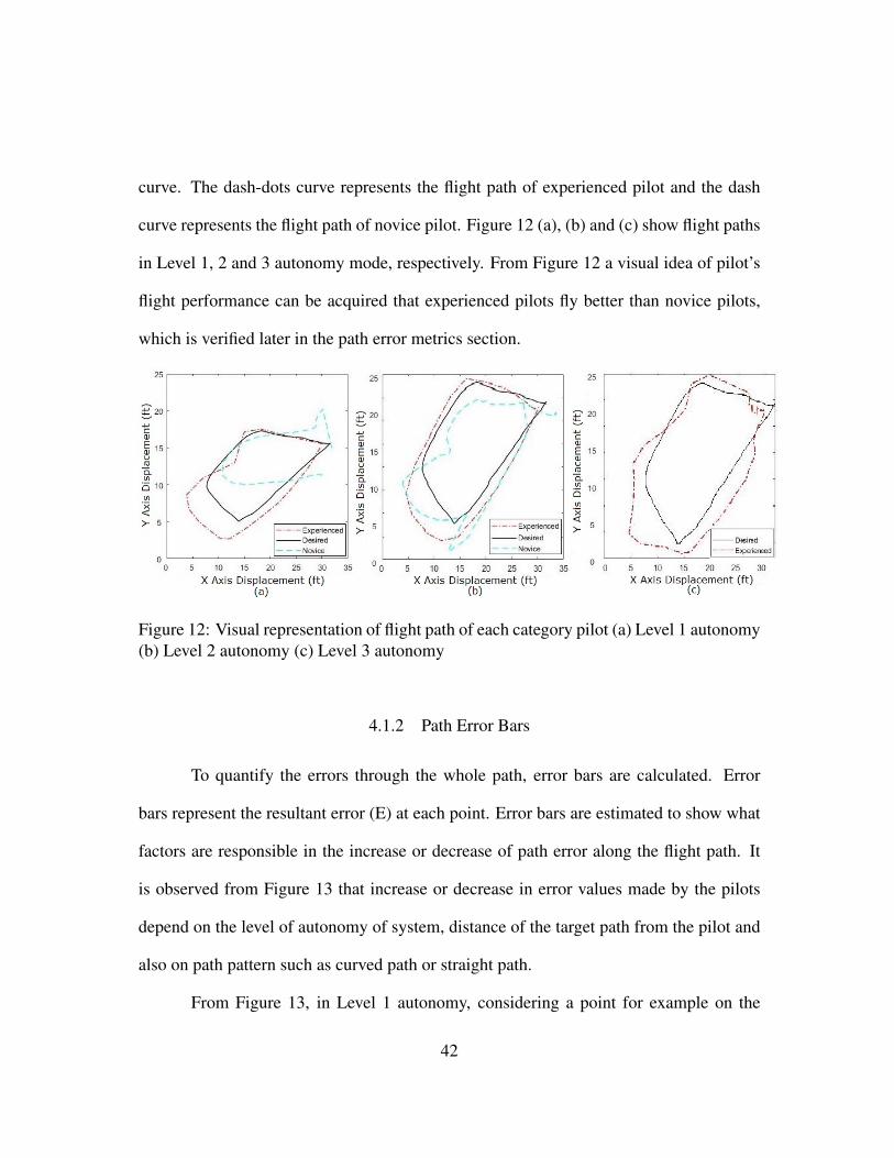
curve. The dash-dots curve represents the flight path of experienced pilot and the dash
curve represents the flight path of novice pilot. Figure 12 (a), (b) and (c) show flight paths
in Level 1, 2 and 3 autonomy mode, respectively. From Figure 12 a visual idea of pilot’s
flight performance can be acquired that experienced pilots fly better than novice pilots,
which is verified later in the path error metrics section.
Figure 12: Visual representation of flight path of each category pilot (a) Level 1 autonomy(b) Level 2 autonomy (c) Level 3 autonomy
4.1.2 Path Error Bars
To quantify the errors through the whole path, error bars are calculated. Error
bars represent the resultant error (E) at each point. Error bars are estimated to show what
factors are responsible in the increase or decrease of path error along the flight path. It
is observed from Figure 13 that increase or decrease in error values made by the pilots
depend on the level of autonomy of system, distance of the target path from the pilot and
also on path pattern such as curved path or straight path.
From Figure 13, in Level 1 autonomy, considering a point for example on the
42
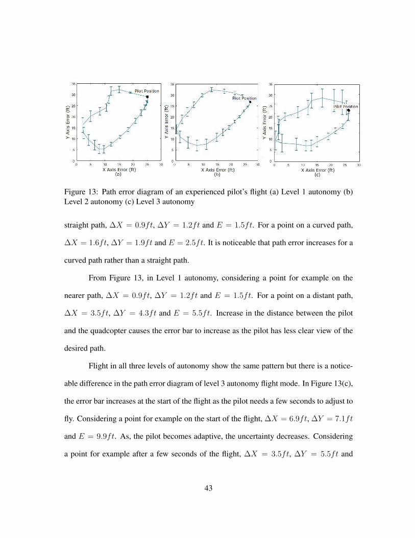
Figure 13: Path error diagram of an experienced pilot’s flight (a) Level 1 autonomy (b)Level 2 autonomy (c) Level 3 autonomy
straight path, ∆X = 0.9ft, ∆Y = 1.2ft and E = 1.5ft. For a point on a curved path,
∆X = 1.6ft, ∆Y = 1.9ft and E = 2.5ft. It is noticeable that path error increases for a
curved path rather than a straight path.
From Figure 13, in Level 1 autonomy, considering a point for example on the
nearer path, ∆X = 0.9ft, ∆Y = 1.2ft and E = 1.5ft. For a point on a distant path,
∆X = 3.5ft, ∆Y = 4.3ft and E = 5.5ft. Increase in the distance between the pilot
and the quadcopter causes the error bar to increase as the pilot has less clear view of the
desired path.
Flight in all three levels of autonomy show the same pattern but there is a notice-
able difference in the path error diagram of level 3 autonomy flight mode. In Figure 13(c),
the error bar increases at the start of the flight as the pilot needs a few seconds to adjust to
fly. Considering a point for example on the start of the flight, ∆X = 6.9ft, ∆Y = 7.1ft
and E = 9.9ft. As, the pilot becomes adaptive, the uncertainty decreases. Considering
a point for example after a few seconds of the flight, ∆X = 3.5ft, ∆Y = 5.5ft and
43

E = 6.5ft. This estimation shows the difference between Level 3 and other two flight
autonomy levels as the error is low at the start of the flight and increases after few seconds.
The representative plot of Figure 13 for an experienced pilot supports the plots
of all other experienced pilots. All the novice pilots show same flight pattern for Level
1 and 2 autonomy. As novice pilots could not fly in the Level 3 autonomy mode, only
experience pilot’s flight test results are shown for Level 3 flight autonomy in Figure 13(c).
4.1.3 Path Error Metrics
Mean value of path error (ME), standard deviation of path error (SD) and root
mean square value of path error (RMSE), are calculated for the quantification of pilot
and quadcopter performance in time domain. Each pilot flew the quadcopter three times
in each autonomy level (total of nine flights). The error metrics in Table 4, Table 5 and
Table 6 are shown as (average ± uncertainty) format.
The mean value of path error is calculated to show the average performance of
a pilot through the whole path following the task. From Table 4, considering Level 1
autonomy flight mode, mean value of error for flight test of pilot 1 (representative of
experienced pilots) is 3.3 ± 0.1 and mean value of error for flight test of pilot 7 (rep-
resentative of novice pilots) is 11.7 ± 1.8. Considering a specific fight autonomy level,
the value of average and uncertainty increase as the pilot level changes from experienced
to novice pilots. Increase in the average of error indicates that novice pilots have higher
error than experienced pilots.
Considering a specific pilot, the mean value of path error for flight test of pilot
44
1 (representative of experienced pilots) is 3.3 ± 0.1 in Level 1 autonomy, 3.6 ± 0.2 in
Level 2 autonomy and 6.2 ± 0.4 in Level 3 autonomy. Considering a specific pilot,
value of average and uncertainty increases from Level 1 to Level 2 to Level 3 autonomy.
Irrespective of pilot experience level, the mean value of path error increases as autonomy
level of the aircraft decreases.
The mean value of path error is considered as a predictor during the modeling for
pilot experience level and UAV autonomy level modeling to identify if the mean value of
path error is a result of pilot performance or UAV performance or both.
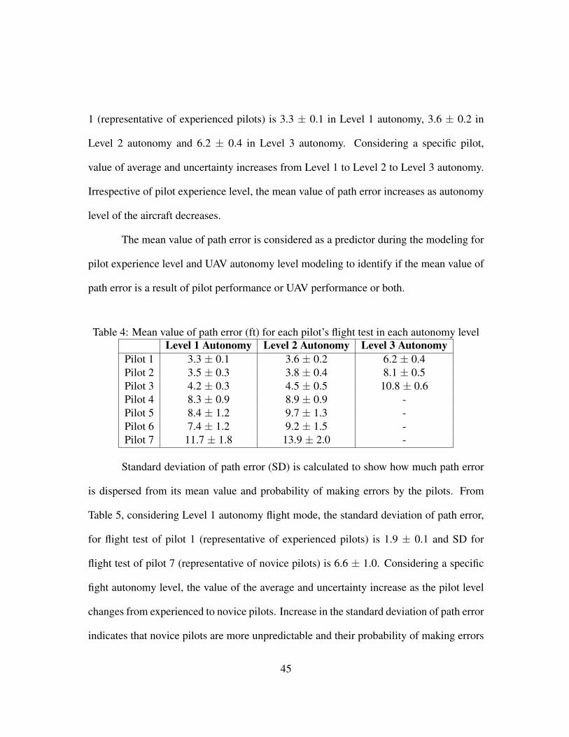
Table 4: Mean value of path error (ft) for each pilot’s flight test in each autonomy levelLevel 1 Autonomy Level 2 Autonomy Level 3 Autonomy
Pilot 1 3.3 ± 0.1 3.6 ± 0.2 6.2 ± 0.4Pilot 2 3.5 ± 0.3 3.8 ± 0.4 8.1 ± 0.5Pilot 3 4.2 ± 0.3 4.5 ± 0.5 10.8 ± 0.6Pilot 4 8.3 ± 0.9 8.9 ± 0.9 -Pilot 5 8.4 ± 1.2 9.7 ± 1.3 -Pilot 6 7.4 ± 1.2 9.2 ± 1.5 -Pilot 7 11.7 ± 1.8 13.9 ± 2.0 -
Standard deviation of path error (SD) is calculated to show how much path error
is dispersed from its mean value and probability of making errors by the pilots. From
Table 5, considering Level 1 autonomy flight mode, the standard deviation of path error,
for flight test of pilot 1 (representative of experienced pilots) is 1.9 ± 0.1 and SD for
flight test of pilot 7 (representative of novice pilots) is 6.6 ± 1.0. Considering a specific
fight autonomy level, the value of the average and uncertainty increase as the pilot level
changes from experienced to novice pilots. Increase in the standard deviation of path error
indicates that novice pilots are more unpredictable and their probability of making errors
45

is higher than the experienced pilots.
Considering a specific pilot, standard deviation of path error for flight tests from
pilot 1 (representative of experienced pilots) is 1.9± 0.1 in Level 1 autonomy, 2.1± 0.2 in
Level 2 autonomy and 3.8 ± 0.3 in Level 3 autonomy. Considering a specific pilot, value
of average and uncertainty increases from Level 1 to Level 2 to Level 3 autonomy. Irre-
spective of pilot experience level, standard deviation of path error increases as autonomy
level of the aircraft decreases.
The standard deviation of path error (SD) is considered as a predictor during the
modeling for pilot experience level and UAV autonomy level modeling to identify if the
SD of path error is a result of pilot performance or UAV performance or both.
Table 5: Standard Deviation of path error (ft) for each pilot’s flight test in each autonomylevel
Level 1 Autonomy Level 2 Autonomy Level 3 AutonomyPilot 1 1.9 ± 0.1 2.1 ± 0.2 3.8 ± 0.3Pilot 2 1.7 ± 0.2 2.3 ± 0.2 2.8 ± 0.3Pilot 3 2.2 ± 0.2 2.8 ± 0.3 6.4 ± 0.4Pilot 4 2.5 ± 0.5 7.2 ± 0.5 -Pilot 5 4.8 ± 0.6 6.1 ± 0.8 -Pilot 6 5.7 ± 0.6 6.2 ± 0.9 -Pilot 7 6.6 ± 1.0 7.0 ± 1.1 -
The root mean square value of path error (RMSE) is calculated to show the vari-
ance of error. RMSE gives relatively high weight to large errors. From Table 6, con-
sidering Level 1 autonomy flight mode, RMSE for flight test of pilot 1 (representative
of experienced pilots) is 3.6 ± 0.3 and RMSE for flight test of pilot 7 (representative of
novice pilots) is 14.8 ± 2.1. Considering a specific fight autonomy level, the value of
46
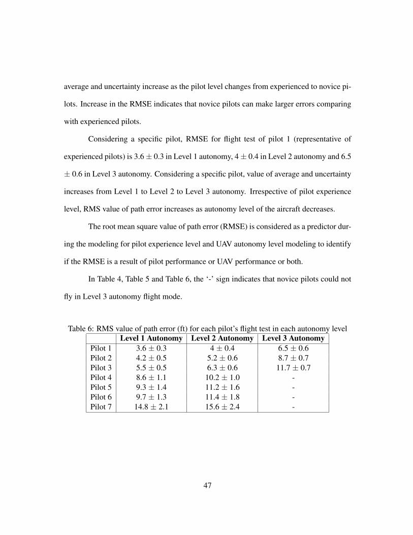
average and uncertainty increase as the pilot level changes from experienced to novice pi-
lots. Increase in the RMSE indicates that novice pilots can make larger errors comparing
with experienced pilots.
Considering a specific pilot, RMSE for flight test of pilot 1 (representative of
experienced pilots) is 3.6± 0.3 in Level 1 autonomy, 4± 0.4 in Level 2 autonomy and 6.5
± 0.6 in Level 3 autonomy. Considering a specific pilot, value of average and uncertainty
increases from Level 1 to Level 2 to Level 3 autonomy. Irrespective of pilot experience
level, RMS value of path error increases as autonomy level of the aircraft decreases.
The root mean square value of path error (RMSE) is considered as a predictor dur-
ing the modeling for pilot experience level and UAV autonomy level modeling to identify
if the RMSE is a result of pilot performance or UAV performance or both.
In Table 4, Table 5 and Table 6, the ‘-’ sign indicates that novice pilots could not
fly in Level 3 autonomy flight mode.
Table 6: RMS value of path error (ft) for each pilot’s flight test in each autonomy levelLevel 1 Autonomy Level 2 Autonomy Level 3 Autonomy
Pilot 1 3.6 ± 0.3 4 ± 0.4 6.5 ± 0.6Pilot 2 4.2 ± 0.5 5.2 ± 0.6 8.7 ± 0.7Pilot 3 5.5 ± 0.5 6.3 ± 0.6 11.7 ± 0.7Pilot 4 8.6 ± 1.1 10.2 ± 1.0 -Pilot 5 9.3 ± 1.4 11.2 ± 1.6 -Pilot 6 9.7 ± 1.3 11.4 ± 1.8 -Pilot 7 14.8 ± 2.1 15.6 ± 2.4 -
47

4.1.4 Accuracy & Precision
In the average± uncertainty format for ME, SD and RMSE, the average indicates
the accuracy of the pilot performance as well as the unmanned aircraft system. Lower av-
erage values indicate that experienced pilots and Level 1 autonomy of unmanned aircraft
have higher accuracy. Higher average values of error metrics indicate that novice pilots
and Level 3 autonomy of unmanned aircraft have lower accuracy. The uncertainty value
indicates the precision or repeatability of a pilot’s performance. Lower value of uncer-
tainty indicates that the pilot is precise in accomplishing the task or pilots’ performance
is repeatable as for experience pilots. As the uncertainty increases, pilot’s precision de-
creases as for novice pilots. The average ± uncertainty format of ME, SD and RMSE, is
useful to differentiate pilot and quadcopter performance individually based on accuracy
and precision characteristic.
4.2 Frequency domain analysis
This section includes variables derived from transfer function modeling in fre-
quency domain such as transfer function order, reliable frequency, coherence function
and stability margin criteria. The frequency domain variables are used to evaluate and
quantify pilot and quadcopter performance considering the frequency response of the sys-
tem.
48
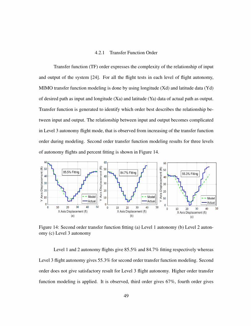
4.2.1 Transfer Function Order
Transfer function (TF) order expresses the complexity of the relationship of input
and output of the system [24]. For all the flight tests in each level of flight autonomy,
MIMO transfer function modeling is done by using longitude (Xd) and latitude data (Yd)
of desired path as input and longitude (Xa) and latitude (Ya) data of actual path as output.
Transfer function is generated to identify which order best describes the relationship be-
tween input and output. The relationship between input and output becomes complicated
in Level 3 autonomy flight mode, that is observed from increasing of the transfer function
order during modeling. Second order transfer function modeling results for three levels
of autonomy flights and percent fitting is shown in Figure 14.
Figure 14: Second order transfer function fitting (a) Level 1 autonomy (b) Level 2 auton-omy (c) Level 3 autonomy
Level 1 and 2 autonomy flights give 85.5% and 84.7% fitting respectively whereas
Level 3 flight autonomy gives 55.3% for second order transfer function modeling. Second
order does not give satisfactory result for Level 3 flight autonomy. Higher order transfer
function modeling is applied. It is observed, third order gives 67%, fourth order gives
49

83.1% and fifth order gives 72% fitting. Applying for all the flight test results in Level 3
flight autonomy, fourth order transfer function modeling is considered as the best model
to describe the input-output relationship. Actual and model output with percent fitting is
shown in Figure 15.
Figure 15: Fourth order transfer function fitting for Level 3 autonomy
Transfer function orders in frequency domain helps to distinguish between Level
3 autonomy flight mode from Level 1 and 2. Fourth order transfer function gives satisfac-
tory fitting for Level 3 autonomy flight mode rather than second order transfer function
for Level 1 and 2, it is observed that the complexity of input-output relationship of Level
3 autonomy mode is higher than Level 1 and 2 flight autonomy mode.
4.2.2 Frequency Response Identification
In this section, Bode plots on raw data and the corresponding coherence plots are
shown to distinguish among three levels of flight autonomy based on frequency response
50
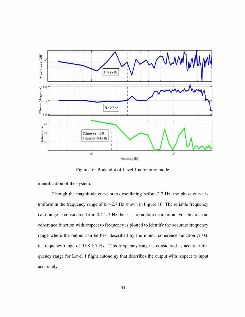
Figure 16: Bode plot of Level 1 autonomy mode
identification of the system.
Though the magnitude curve starts oscillating before 2.7 Hz, the phase curve is
uniform in the frequency range of 0.4-2.7 Hz shown in Figure 16. The reliable frequency
(Fr) range is considered from 0.4-2.7 Hz, but it is a random estimation. For this reason,
coherence function with respect to frequency is plotted to identify the accurate frequency
range where the output can be best described by the input. coherence function > 0.6
in frequency range of 0.98-1.7 Hz. This frequency range is considered as accurate fre-
quency range for Level 1 flight autonomy that describes the output with respect to input
accurately.
51

Figure 17: Bode plot of Level 2 autonomy mode
For Level 2 autonomy flight mode, the random estimation for reliable frequency
(Fr) range is considered from 0.4-2.7 Hz shown in Figure 17. To identify accurate fre-
quency range coherence function plot shows that coherence function > 0.6 in frequency
range of 0.98-2.7 Hz. In this frequency range the output is best described by the input.
For Level 3 autonomy flight mode, reliable frequency (Fr) range is considered
from 0.4-3.5 Hz shown in Figure 18. Reliable frequency range is a random estimation
from the bode plots. To identify accurate frequency range coherence function is plotted
and it shows that coherence function > 0.6 in frequency range of 0.98-3 Hz for Level 3
flight autonomy. In this frequency range the output is best described by the input of the
system.
52
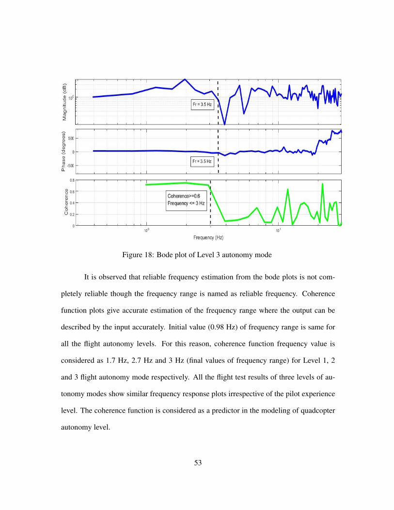
Figure 18: Bode plot of Level 3 autonomy mode
It is observed that reliable frequency estimation from the bode plots is not com-
pletely reliable though the frequency range is named as reliable frequency. Coherence
function plots give accurate estimation of the frequency range where the output can be
described by the input accurately. Initial value (0.98 Hz) of frequency range is same for
all the flight autonomy levels. For this reason, coherence function frequency value is
considered as 1.7 Hz, 2.7 Hz and 3 Hz (final values of frequency range) for Level 1, 2
and 3 flight autonomy mode respectively. All the flight test results of three levels of au-
tonomy modes show similar frequency response plots irrespective of the pilot experience
level. The coherence function is considered as a predictor in the modeling of quadcopter
autonomy level.
53
4.2.3 Stability Margin Criteria
Gain margin (Gm) and phase margin (Pm) values for each pilot’s flight testing in
each autonomy level are shown in Table 7. Each pilot has flown the quadcopter three
times in each autonomy level. Phase margin values for experienced pilots and gain and
phase margin values for novice pilots are expressed in (average ± uncertainty) format. In
case of infinity gain margin values, uncertainty is not applicable.
For experienced pilots, infinity gain margin is achievable in all the three levels of
flight autonomy. Table 7 shows that for Pilot 1, 2 and 3 (experienced group) gain margin
is infinity in all three levels of flight autonomy. But, infinity gain margin is not achievable
for novice pilots in any of the flight autonomy level that is visible in Table 7 for Pilot
4,5,6 and 7. Infinity gain margin denotes the system will not go unstable or unbalanced
under the tested conditions. This criteria is helpful to distinguish between experienced
and novice pilots.
Although a difference is visible between experienced and novice pilots’ perfor-
mance from gain margin, phase margin does not show such distinction. From Table 7, in
Level 1 autonomy, Pilot 2 shows phase margin of 55.9 ± 5 degrees, but for Pilot 5 this
value is 126 ± 9.8 degrees. Pilot 7 has a phase margin of 10.9 ± 10.6 degrees, for Level
1 autonomy. This random values are also noticeable for Level 2 flight autonomy. Gain
and phase margin values are empty for novice pilots in case of Level 3 autonomy as they
could not fly in this mode. Phase margin values increase or decrease irrespective of the
pilot experience level and unmanned aircraft autonomy level, phase margin values are not
helpful to distinguish between experienced and novice pilots and different levels of flight
54

autonomy. For this reason, phase margin is not considered as an explanatory variable or
predictor during dependency test and modeling.
Table 7: Gain Margin(dB) and Phase Margin (degree) for each pilot’s flight test in eachautonomy level
Level 1 Autonomy Level 2 Autonomy Level 3 AutonomyGm(dB) Pm(degree) Gm(dB) Pm(degree) Gm(dB) Pm(degree)
Pilot 1 Inf Inf Inf 160.2 ± 5 Inf -25.5 ± 12Pilot 2 Inf 55.9 ± 5 Inf 50.4 ± 5.6 Inf -11.1 ± 12.5Pilot 3 Inf 25.3 ± 5 Inf 157 ± 7 Inf -26.9 ± 11Pilot 4 12.5 ± 8.2 27.3 ± 9.5 -84.7 ± 8 51.3 ± 7 - -Pilot 5 7.84 ± 10.5 126 ± 9.8 22.9 ± 11.9 1.33 ± 10.7 - -Pilot 6 21.5 ± 10.9 -2.66 ± 15.9 11.4 ± 9.5 23 ± 11.2 - -Pilot 7 25.1 ± 12.5 10.9 ± 10.6 2.55 ± 7.3 2.14 ± 8.9 - -
4.3 Cooper-Harper Rating Scale
After completing each flight test, the pilots were given the abbreviated version
of Cooper-Harper rating scale shown in Table 3 to give rating to the unmanned aircraft
system. Each pilot has used this table nine times, three times per single autonomy level
flight testing. An individual pilot has given the same rating for all three flights in a specific
autonomy level, that is expressed by a number between 1-10 without any uncertainty
range shown in Table 8.
The experienced pilots rate the unmanned system as Level 1 (C-H rating range
from 1 to 3) for both Level 1 and 2 autonomy modes. They can achieve the desired
performance from the quadcopter and feel comfortable while completing the task in these
autonomy levels. But, in level 3 autonomy mode, C-H rating degrades to Level 2 (C-H
55

Table 8: Pilot given C-H rating of UAV in different flight modesLevel 1 Autonomy Level 2 Autonomy Level 3 Autonomy
Pilot 1 2 2 5Pilot 2 3 2 7Pilot 3 3 3 4Pilot 4 5 4 10Pilot 5 5 5 10Pilot 6 5 5 10Pilot 7 8 7 10
rating range from 4 to 6) and Level 3 (C-H rating range from 7 to 9), meaning UAV is
objectionable, needs improvement and not suitable enough to accomplish the task.
In the case of novice pilots, either the rating for UAV is Level 2 (C-H rating range
from 4 to 6) or Level 3 (C-H rating range from 7 to 9) in both Level 1 and 2 autonomy
modes. The novice pilots object the unmanned system while flying in Level 1 and 2
autonomy mode and after the flight in Level 3 autonomy mode, all of the novice pilots
give 10 to the system, denoting that in this mode the quadcopter is not controllable.
From the results in Table 12, it is observed that C-H rating of UAV degrades
for novice pilots comparing with the experienced pilots irrespective of flight autonomy
level. The degradation is a criteria to distinguish between two categories of pilots. For an
individual pilot, experienced or novice, C-H rating of the UAV degrades from Level 1 to
2 to 3 autonomy flight mode. This distinction is used to categorize three levels of flight
autonomy irrespective of the pilot experience level.
4.4 Pilot Experience Level Modeling
The pilot level modeling results are divided into three steps.
56

Step 1: Variable dependency test results.
Step 2: Parameter estimation results using binary logistic regression.
Step 3: Verification test case results an pilot level modeling.
4.4.1 Variable Dependency Test
As pilot experience level has two categories, independent sample t test is per-
formed to identify significant relation of pilot level with time, frequency domain and
Cooper-Harper rating variables. Table 9 shows that flight variables such as flight auton-
omy level, transfer function order and coherence function have a P value greater than
0.05. These three variables do not have significant relationship with pilot experience level
and are not considered as independent variables in the modeling of pilot experience level .
The other six variables have a P value < 0.05, showing significant relationship with pilot
experience level and are considered as independent variables in the modeling.
Table 9: P value of independent sample t-test for pilot experience levelIndependent Variable : Pilot Experience Level
Dependent Variables P ValueFlight Autonomy Level 1.000
TF Order 1.000Coherence Function 1.000
ME 0.031SD 0.022
RMSE 0.027Uncertainty 0.048Gain Margin 0.000
C-H 0.004
57

4.4.2 Binary Logistic Regression
Parameter estimation for pilot level modeling is shown in Table 10 . Exponential
of coefficients or parameters, Exp(β) are known as odds ratio. From Table 10, the odds
ratio of gain margin is > 1 and for all the other predictors it is < 1. So, if the value of
stability margin is increased, the outcome for the pilot level will fall into the comparison
group, experienced. If values of all other independent variables are increased, the output
will fall into the referent group, novice. Decrease in the value of stability margin will
result outcome to be referent group, novice and decrease in all other variables will result
the outcome to be comparison group, experienced.
Table 10: Parameter estimation for pilot level modeling
Pilot Level (Referent Group : Novice) Independent Variables Parameter, β Exp(β)Comparison Group: Mean of Error -0.843 0.43
Experienced SD -0.086 0.917RMSE -0.691 0.501
Uncertainty -0.115 0.891Gain Margin 0.006 1.006
C-H -0.351 0.704
4.5 UAV Autonomy Level Modeling
The UAV autonomy level modeling results are divided into three steps.
Step 1: Variable dependency test results.
Step 2: Parameter estimation results using multinomial logistic regression.
Step 3: Verification test case results and level of autonomy of UAV modeling.
58
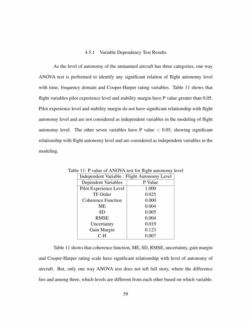
4.5.1 Variable Dependency Test Results
As the level of autonomy of the unmanned aircraft has three categories, one way
ANOVA test is performed to identify any significant relation of flight autonomy level
with time, frequency domain and Cooper-Harper rating variables. Table 11 shows that
flight variables pilot experience level and stability margin have P value greater than 0.05.
Pilot experience level and stability margin do not have significant relationship with flight
autonomy level and are not considered as independent variables in the modeling of flight
autonomy level. The other seven variables have P value < 0.05, showing significant
relationship with flight autonomy level and are considered as independent variables in the
modeling.
Table 11: P value of ANOVA test for flight autonomy levelIndependent Variable : Flight Autonomy LevelDependent Variables P Value
Pilot Experience Level 1.000TF Order 0.025
Coherence Function 0.000ME 0.004SD 0.005
RMSE 0.004Uncertainty 0.019Gain Margin 0.123
C-H 0.007
Table 11 shows that coherence function, ME, SD, RMSE, uncertainty, gain margin
and Cooper-Harper rating scale have significant relationship with level of autonomy of
aircraft. But, only one way ANOVA test does not tell full story, where the difference
lies and among three, which levels are different from each other based on which variable.
59

For this reason, post hoc test using Tukey method is done to identify actual difference
between two groups separately ( between Level 1 and 2, Level 2 and 3, Level 3 and 1)
flight autonomy levels, based on specific variables.
Table 12: Post hoc test for flight autonomy level
Dependent Variables Independent Variables Independent Variables P ValuePilot Experience Level Level 1 Autonomy Level 2 Autonomy 0.999
Level 3 Autonomy 0.999Level 2 Autonomy Level 3 Autonomy 0.999
TF Order Level 1 Autonomy Level 2 Autonomy 0.999Level 3 Autonomy 0.027
Level 2 Autonomy Level 3 Autonomy 0.028Coherence Function Level 1 Autonomy Level 2 Autonomy 0.000
Level 3 Autonomy 0.000Level 2 Autonomy Level 3 Autonomy 0.000
Mean of Error Level 1 Autonomy Level 2 Autonomy 0.999Level 3 Autonomy 0.008
Level 2 Autonomy Level 3 Autonomy 0.009SD of Error Level 1 Autonomy Level 2 Autonomy 0.983
Level 3 Autonomy 0.008Level 2 Autonomy Level 3 Autonomy 0.012
RMSE Level 1 Autonomy Level 2 Autonomy 0.999Level 3 Autonomy 0.008
Level 2 Autonomy Level 3 Autonomy 0.009Uncertainty Level 1 Autonomy Level 2 Autonomy 1.000
Level 3 Autonomy 0.034Level 2 Autonomy Level 3 Autonomy 0.036
Gain Margin Level 1 Autonomy Level 2 Autonomy 0.993Level 3 Autonomy 0.190
Level 2 Autonomy Level 3 Autonomy 0.158C-H Level 1 Autonomy Level 2 Autonomy 0.744
Level 3 Autonomy 0.037Level 2 Autonomy Level 3 Autonomy 0.008
Post hoc test shows the significant difference between two groups when number
60
of groups are more than two. From Table 12 only the coherence function can distinguish
between Level 1 and 2 autonomy flight mode showing P value < 0.05. Other variables do
not show significant difference between Level 1 and 2 autonomy flight mode, showing P
value ≥ 0.05. Except pilot experience level and gain margin values (showing P value ≥
0.05), all the other variables show significant relationship (P value < 0.05) to distinguish
Level 3 flight autonomy from Level 1 and 2 flight autonomy modes. For this reason,
while modeling the flight autonomy level using multinomial logistic regreesion, Level
3 autonomy mode is considered as referent group and Level 1 and 2 are considered as
comparison group 1 and 2 respectively.
4.5.2 Multinomial Logistic Regression Modeling
Flight autonomy modeling results are shown in Table 13. Based on the post hoc
test results, Level 3 autonomy is considered as referent group and Level 1 and 2 autonomy
are considered as comparison group 1 and 2 respectively. For both Level 1 and 2, the
odds ratio for all the parameters is < 1. While comparing autonomy level 1 and 3, if
values of each of the independent variables are increased individually, the output will
fall into the referent group, Level 3 flight autonomy. Decrease in the values of each
of the independent variables individually will result outcome to be comparison group 1,
Level 1 flight autonomy. Same scenario is observed, while comparing level 2 and 3. If
values of each of the independent variables are increased individually, the output will fall
into the referent group, Level 3 flight autonomy. Decrease in the values of each of the
independent variables individually will result outcome to be comparison group 2, Level 2
61

flight autonomy
Table 13: Parameter estimation for flight autonomy level modeling
Flight Autonomy (Referent Group : Level 3) Independent Variables Parameter, β Exp(β)Comparison Group 1: Mean of Error -1.058 0.347
Level 1 SD -0.645 0.525RMSE -0.938 0.391
Uncertainty -0.947 0.388TF Order -0.025 0.975
Coherence Function -1.259 0.284C-H -0.359 0.704
Comparison Group 2: Mean of Error -1.783 0.168Level 2 SD -0.352 0.703
RMSE -1.306 0.271Uncertainty -0.834 0.434TF Order -0.025 0.975
Coherence Function -2.292 0.101C-H -0.269 0.764
Comparison of different levels of autonomy, with respect to increase or decrease of
independent variables helps to differentiate between Level 3 flight autonomous mode from
Level 1 and 2 flight modes. MLR test is useful to differentiate between flight autonomy
levels based on the flight data analysis and variation of values of predictor variables.
4.6 Verification Test Case
To strengthen the analysis and modeling of evaluation of pilot and quadcopter
performance, a verification flight test was conducted. Flight data was collected from an
eighth pilot’s flight test. After the flight testing, the pilot gives rating to the UAV using
abbreviated version of modified Cooper-Harper rating scale. Time and frequency domain
analysis is done on the collected flight test data. The pilot was unknown about the flight
62
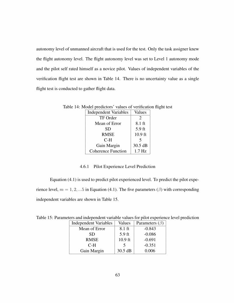
autonomy level of unmanned aircraft that is used for the test. Only the task assigner knew
the flight autonomy level. The flight autonomy level was set to Level 1 autonomy mode
and the pilot self rated himself as a novice pilot. Values of independent variables of the
verification flight test are shown in Table 14. There is no uncertainty value as a single
flight test is conducted to gather flight data.
Table 14: Model predictors’ values of verification flight testIndependent Variables Values
TF Order 2Mean of Error 8.1 ft
SD 5.9 ftRMSE 10.9 ft
C-H 5Gain Margin 30.5 dB
Coherence Function 1.7 Hz
4.6.1 Pilot Experience Level Prediction
Equation (4.1) is used to predict pilot experienced level. To predict the pilot expe-
rience level, m = 1, 2, ...5 in Equation (4.1). The five parameters (β) with corresponding
independent variables are shown in Table 15.
Table 15: Parameters and independent variable values for pilot experience level predictionIndependent Variables Values Parameters (β)
Mean of Error 8.1 ft -0.843SD 5.9 ft -0.086
RMSE 10.9 ft -0.691C-H 5 -0.351
Gain Margin 30.5 dB 0.006
63
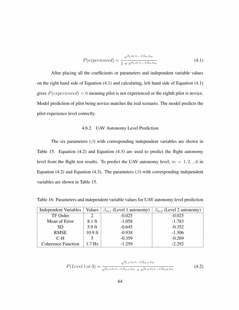
P (experienced) =eβ1.x1+...+βm.xm
1 + eβ1.x1+...+βm.xm(4.1)
After placing all the coefficients or parameters and independent variable values
on the right hand side of Equation (4.1) and calculating, left hand side of Equation (4.1)
gives P (experienced) = 0 meaning pilot is not experienced or the eighth pilot is novice.
Model prediction of pilot being novice matches the real scenario. The model predicts the
pilot experience level correctly.
4.6.2 UAV Autonomy Level Prediction
The six parameters (β) with corresponding independent variables are shown in
Table 15. Equation (4.2) and Equation (4.3) are used to predict the flight autonomy
level from the flight test results. To predict the UAV autonomy level, m = 1, 2, ...6 in
Equation (4.2) and Equation (4.3). The parameters (β) with corresponding independent
variables are shown in Table 15.
Table 16: Parameters and independent variable values for UAV autonomy level prediction
Independent Variables Values βm,1 (Level 1 autonomy) βm,2 (Level 2 autonomy)TF Order 2 -0.025 -0.025
Mean of Error 8.1 ft -1.058 -1.783SD 5.9 ft -0.645 -0.352
RMSE 10.9 ft -0.938 -1.306C-H 5 -0.359 -0.269
Coherence Function 1.7 Hz -1.259 -2.292
P (Level 1 or 3) =eβ1,1.x1+...+βm,1.xm
eβ1,1.x1+...+βm,1.xm + eβ1,2.x1+...+βm,2.xm(4.2)
64
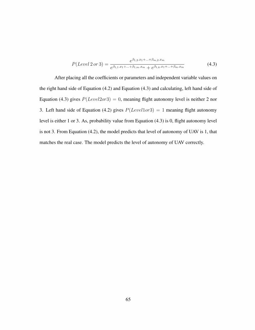
P (Level 2 or 3) =eβ1,2.x1+...+βm,2.xm
eβ1,1.x1+...+β1,m.xm + eβ1,k.x1+...+βm.xm(4.3)
After placing all the coefficients or parameters and independent variable values on
the right hand side of Equation (4.2) and Equation (4.3) and calculating, left hand side of
Equation (4.3) gives P (Level2or3) = 0, meaning flight autonomy level is neither 2 nor
3. Left hand side of Equation (4.2) gives P (Level1or3) = 1 meaning flight autonomy
level is either 1 or 3. As, probability value from Equation (4.3) is 0, flight autonomy level
is not 3. From Equation (4.2), the model predicts that level of autonomy of UAV is 1, that
matches the real case. The model predicts the level of autonomy of UAV correctly.
65
CHAPTER 5
CONCLUSION
This work demonstrates an evaluation technique of pilot and quadcopter perfor-
mance by analyzing the flight test results. Research was done before to evaluate pilot per-
formance based on the workload. But, individually pilot and unmanned aircraft system
evaluation is necessary as either pilot failure or UAV failure can cause severe accidents.
Before assigning a task, both pilot and UAV evaluation will help to determine if the pilot
can accomplish a task with the assigned unmanned aircraft system. The evaluation tech-
nique serves this purpose and would be useful for training pilots to fulfill the task avoiding
any undesired situation.
Outdoor flight testing based on a specific mission task helps to gather flight data
corresponding to real life experience. On gathered flight data, time and frequency domain
analysis approach are used that help to understand system behavior in two domains in-
dividually. In the time domain analysis, three error metrics represent the full scenario of
pilot and quadcopter performance based on path errors. All the three error metrics show
better performance from experienced pilots and Level 1 flight mode with highest level of
autonomy. Frequency domain analysis is done to understand frequency response of the
system. System complexity is analyzed from transfer function orders that expresses Level
3 autonomy flight is more complex than Level 1 and 2 autonomy mode. Coherence func-
tion shows that Level 3 autonomous mode is faster than Level 1 and 2 with a wider range
66
of frequency response where the output can be described by the input of the system cor-
rectly. Stability gain margin criteria distinguishes between experienced and novice pilots
analyzing flight stability performance where infinity gain margin is common for experi-
enced pilots in all three flight modes but novice pilots do not show this flight performance.
After the flight testing, pilots give rating to the UAV expressing ease of control of the sys-
tem. Dependency test is performed on time domain variables, frequency domain variables
and Cooper-Harper rating of UAV and significant variables are considered as predictors
for modeling pilot and quadcopter performance. Model developed from flight test results
to predict pilot and quadcopter performance is useful to identify the outcome based on the
changes of predictor’s values. A verification test case strengthens the established model
from a single flight test result when prediction of the model for both pilot experience
level and quadcopter performance level matches the real life known condition of pilot and
quadcopter.
Though some limitations such as GPS accuracy is not great, lower number of pi-
lots and only one unmanned aircraft system, the evaluation technique developed to quan-
tify pilot and quadcopter performance shows a path to train pilots to accomplish a task
with an assigned unmanned aircraft system by analyzing the flight test results.
67

CHAPTER 6
FUTURE WORK
This research work is completed with seven pilots and one unmanned aircraft
system. Though, established model is strengthened by a test case, continuation of this
work includes a larger number of pilots (approximately 20) and different types of UAVs
(multi-rotor, fixed wing, single-rotor helicopter,fixed-wing hybrid VTOL etc.). Flight
testing with larger number of pilots and UAVs will make the model a standard for training
pilots of different levels and evaluate capabilities of UAVs to work in various situations.
68

REFERENCE LIST
[1] M Christopher Cotting. Uav performance rating scale based on the cooper-harper
piloted rating scale. In 49th AIAA Aerospace Sciences Meeting including the New
Horizons Forum and Aerospace Exposition, page 923, 2011.
[2] Martin Neubauer, Georg Gunther, and Konrad Fullhas. Structural design aspects
and criteria for military uav. Technical report, EUROPEAN AERONAUTIC
DEFENCE AND SPACE (EADS) MUNICH (GERMANY), 2007.
[3] Tim Hutchings, Susan Jeffryes, and SJ Farmer. Architecting uav sense & avoid
systems. In Autonomous Systems, 2007 Institution of Engineering and Technology
Conference on, pages 1–8. IET, 2007.
[4] Guohao Li, Matthias Mueller, Vincent Casser, Neil Smith, Dominik L Michels, and
Bernard Ghanem. Teaching uavs to race with observational imitation learning.
arXiv preprint arXiv:1803.01129, 2018.
[5] David Gomez-Candon, AI De Castro, and Francisca Lopez-Granados. Assessing
the accuracy of mosaics from unmanned aerial vehicle (uav) imagery for precision
agriculture purposes in wheat. Precision Agriculture, 15(1):44–56, 2014.
[6] Eduard Semsch, Michal Jakob, Dusan Pavlicek, and Michal Pechoucek.
Autonomous uav surveillance in complex urban environments. In Proceedings of
the 2009 IEEE/WIC/ACM International Joint Conference on Web Intelligence and
69

Intelligent Agent Technology-Volume 02, pages 82–85. IEEE Computer Society,
2009.
[7] Md R Haque, M Muhammad, D Swarnaker, and M Arifuzzaman. Autonomous
quadcopter for product home delivery. In Electrical Engineering and Information
& Communication Technology (ICEEICT), 2014 International Conference on,
pages 1–5. IEEE, 2014.
[8] Xin Li and Lian Yang. Design and implementation of uav intelligent aerial
photography system. In Intelligent Human-Machine Systems and Cybernetics
(IHMSC), 2012 4th International Conference on, volume 2, pages 200–203. IEEE,
2012.
[9] Francesco Nex and Fabio Remondino. Uav for 3d mapping applications: a review.
Applied geomatics, 6(1):1–15, 2014.
[10] Ignacio Hernandez, Travis Fields, and John Kevern. Overcoming the challenges of
using unmanned aircraft for bridge inspections. In AIAA Atmospheric Flight
Mechanics Conference, page 3396, 2016.
[11] Stephen R Dixon, Christopher D Wickens, and Dervon Chang. Comparing
quantitative model predictions to experimental data in multiple-uav flight control.
In Proceedings of the Human Factors and Ergonomics Society Annual Meeting,
volume 47, pages 104–108. SAGE Publications Sage CA: Los Angeles, CA, 2003.
70

[12] Cort J Willmott and Kenji Matsuura. Advantages of the mean absolute error (mae)
over the root mean square error (rmse) in assessing average model performance.
Climate research, 30(1):79–82, 2005.
[13] J Martin Bland and Douglas G Altman. Statistics notes: measurement error. Bmj,
312(7047):1654, 1996.
[14] Tianfeng Chai and Roland R Draxler. Root mean square error (rmse) or mean
absolute error (mae)?–arguments against avoiding rmse in the literature.
Geoscientific model development, 7(3):1247–1250, 2014.
[15] Colin R Theodore, Mark B Tischler, and Jason D Colbourne. Rapid
frequency-domain modeling methods for unmanned aerial vehicle flight control
applications. Journal of Aircraft, 41(4):735–743, 2004.
[16] Subodh Bhandari, Richard Colgren, Philipp Lederbogen, and Scott Kowalchuk.
Six-dof dynamic modeling and flight testing of a uav helicopter. In AIAA Modeling
and Simulation Technologies Conference and Exhibit, page 6422, 2005.
[17] Abdellah Mokhtari, Abdelaziz Benallegue, and Boubaker Daachi. Robust feedback
linearization and gh/sub/spl infin//controller for a quadrotor unmanned aerial
vehicle. In Intelligent Robots and Systems, 2005.(IROS 2005). 2005 IEEE/RSJ
International Conference on, pages 1198–1203. IEEE, 2005.
71
[18] Robert K Remple and Mark B Tischler. Aircraft and rotorcraft system
identification: engineering methods with flight-test examples. American Institute of
Aeronautics and Astronautics, 2006.
[19] Z Shafiei and AT Shenton. Frequency-domain design of pid controllers for stable
and unstable systems with time delay. Automatica, 33(12):2223–2232, 1997.
[20] Mujahid Abdulrahim, Justin Dee, and Jason Grzywna. Handling qualities metrics
for small vtol uavs in precision and agile maneuvering tasks. In AIAA Atmospheric
Flight Mechanics Conference, page 1188, 2017.
[21] Douglas C Montgomery, George C Runger, and Norma F Hubele. Engineering
statistics. John Wiley & Sons, 2009.
[22] David G Kleinbaum and Mitchel Klein. Logistic regression: a self-learning text.
Springer Science & Business Media, 2010.
[23] Chanyeong Kwak and Alan Clayton-Matthews. Multinomial logistic regression.
Nursing research, 51(6):404–410, 2002.
[24] Norman S Nise. CONTROL SYSTEMS ENGINEERING, (With CD). John Wiley &
Sons, 2007.
[25] Taeyoung Lee, Melvin Leok, and N Harris McClamroch. Nonlinear robust tracking
control of a quadrotor uav on se (3). Asian Journal of Control, 15(2):391–408,
2013.
72

[26] Wei Lin. Distributed uav formation control using differential game approach.
Aerospace Science and Technology, 35:54–62, 2014.
[27] Haiyang Chao, Marc Baumann, Austin Jensen, YangQuan Chen, Yongcan Cao,
Wei Ren, and Mac McKee. Band-reconfigurable multi-uav-based cooperative
remote sensing for real-time water management and distributed irrigation control.
IFAC Proceedings Volumes, 41(2):11744–11749, 2008.
[28] Stanley M Shinners. Modeling of human operator performance utilizing time series
analysis. IEEE Transactions on Systems, Man, and Cybernetics, (5):446–458,
1974.
[29] Frank Osafo-Charles, Gyan C Agarwal, William D O’neill, and Gerald L Gottlieb.
Application of time-series modeling to human operator dynamics. IEEE
Transactions on Systems, Man, and Cybernetics, 10(12):849–860, 1980.
[30] Luca Bertuccelli, W Beckers, and Mary Cummings. Developing operator models
for uav search scheduling. In AIAA Guidance, Navigation, and Control
Conference, page 7863, 2010.
[31] Diana Donath, Andreas Rauschert, and Axel Schulte. Cognitive assistant system
concept for multi-uav guidance using human operator behaviour models.
HUMOUSa10, 2010.
73
[32] Mary L Cummings, Carl E Nehme, Jacob Crandall, and Paul Mitchell. Predicting
operator capacity for supervisory control of multiple uavs. In Innovations in
Intelligent Machines-1, pages 11–37. Springer, 2007.
[33] Andrei Dorobantu, Ahmet Arda Ozdemir, Kamran Turkoglu, Paul Freeman, Austin
Murch, Bernie Mettler, and Gary Balas. Frequency domain system identification
for a small, low-cost, fixed-wing uav. In AIAA Guidance, Navigation, and Control
Conference, page 6719, 2011.
[34] Keyur Patel and Jayesh Barve. Modeling, simulation and control study for the
quad-copter uav. In Industrial and Information Systems (ICIIS), 2014 9th
International Conference on, pages 1–6. IEEE, 2014.
[35] Bernard Mettler, Takeo Kanade, and Mark Brian Tischler. System identification
modeling of a model-scale helicopter. Carnegie Mellon University, The Robotics
Institute, 2000.
[36] Bernard Mettler, Mark B Tischler, and Takeo Kanade. System identification of
small-size unmanned helicopter dynamics. In Annual Forum Proceedings-
American Helicopter Society, volume 2, pages 1706–1717, 1999.
[37] Yuhu Du, Jiancheng Fang, and Cunxiao Miao. Frequency-domain system
identification of an unmanned helicopter based on an adaptive genetic algorithm.
IEEE Transactions on Industrial Electronics, 61(2):870–881, 2014.
74
[38] Sung K Kim and Dawn M Tilbury. Mathematical modeling and experimental
identification of an unmanned helicopter robot with flybar dynamics. Journal of
robotic systems, 21(3):95–116, 2004.
[39] Daigo Fujiwara, Jinok Shin, Kensaku Hazawa, and Kenzo Nonami. H/sub/spl
infin//hovering and guidance control for autonomous small-scale unmanned
helicopter. In Intelligent Robots and Systems, 2004.(IROS 2004). Proceedings.
2004 IEEE/RSJ International Conference on, volume 3, pages 2463–2468. IEEE,
2004.
[40] Cort J Willmott, Kenji Matsuura, and Scott M Robeson. Ambiguities inherent in
sums-of-squares-based error statistics. Atmospheric Environment, 43(3):749–752,
2009.
[41] Karin Stahl Gunnarsson, Jorgen Hansson, Fredrik Karlsson, Anders Hansson, and
Ragnar Wallin. Clearance of flight control laws using linear fractional
transformations. In AIAA Guidance, Navigation, and Control Conference and
Exhibit, page 4867, 2004.
[42] Kuang-Wei Han and Che-Hsu Chang. Gain margins and phase margins for control
systems with adjustable parameters. Journal of guidance, control, and dynamics,
13(3):404–408, 1990.
[43] Bilal Ahmed and Hemanshu R Pota. Dynamic compensation for control of a rotary
wing uav using positive position feedback. Journal of Intelligent & Robotic
Systems, 61(1-4):43–56, 2011.
75

[44] Jang-Ho Lee, Byoung-Mun Min, and Eung-Tai Kim. Autopilot design of tilt-rotor
uav using particle swarm optimization method. In Control, Automation and
Systems, 2007. ICCAS’07. International Conference on, pages 1629–1633. IEEE,
2007.
[45] Dong-Wan Yoo, Hyon-Dong Oh, Dae-Yeon Won, and Min-Jea Tahk. Dynamic
modeling and stabilization techniques for tri-rotor unmanned aerial vehicles.
International Journal of Aeronautical and Space Sciences, 11(3):167–174, 2010.
[46] George E Cooper and Robert P Harper Jr. The use of pilot rating in the evaluation
of aircraft handling qualities. Technical report, Advisory Group for aerospace
research and development Neuilly-Sur-Seine (France), 1969.
[47] ML Cummings, Kevin Myers, and Stacey D Scott. Modified cooper harper
evaluation tool for unmanned vehicle displays. In Proceedings of UVS Canada:
Conference on Unmanned Vehicle Systems Canada, 2006.
[48] Balaji Krishnapuram, Lawrence Carin, Mario AT Figueiredo, and Alexander J
Hartemink. Sparse multinomial logistic regression: Fast algorithms and
generalization bounds. IEEE Transactions on Pattern Analysis & Machine
Intelligence, (6):957–968, 2005.
[49] Yuan Tian, David Lo, and Chengnian Sun. Drone: Predicting priority of reported
bugs by multi-factor analysis. In 2013 IEEE International Conference on Software
Maintenance, pages 200–209. IEEE, 2013.
76
[50] Anthony P Tvaryanas, William T Thompson, and Stefan H Constable. Human
factors in remotely piloted aircraft operations: Hfacs analysis of 221 mishaps over
10 years. Aviation, space, and environmental medicine, 77(7):724–732, 2006.
[51] Abdallah Zeggada, Farid Melgani, and Yakoub Bazi. A deep learning approach to
uav image multilabeling. IEEE Geoscience and Remote Sensing Letters,
14(5):694–698, 2017.
[52] Karl Kaltenthaler, William Miller, and Christine Fair. The drone war: Pakistani
public attitudes toward american drone strikes in pakistan. In Annual Meetings of
the Midwest Political Science Association, 2013.
[53] Teppo Luukkonen. Modelling and control of quadcopter. Independent research
project in applied mathematics, Espoo, 22, 2011.
[54] M Heryanto, Herwin Suprijono, Bhakti Yudho Suprapto, and Benyamin
Kusumoputro. Attitude and altitude control of a quadcopter using neural network
based direct inverse control scheme. Advanced Science Letters, 23(5):4060–4064,
2017.
[55] Stanisław Anweiler and Dawid Piwowarski. Multicopter platform prototype for
environmental monitoring. Journal of Cleaner Production, 155:204–211, 2017.
[56] Sebastian Madgwick. An efficient orientation filter for inertial and
inertial/magnetic sensor arrays. Report x-io and University of Bristol (UK),
25:113–118, 2010.
77

[57] Alexandra Kuznetsova, Per B Brockhoff, and Rune Haubo Bojesen Christensen.
lmertest package: tests in linear mixed effects models. Journal of Statistical
Software, 82(13), 2017.
[58] Anthony Hilton and Richard Armstrong. Statnote 6: post-hoc anova tests. 2006.

VITA
Muhammad Junayed Hasan Zahed was born on September 1, 1989 in Chittagong,
Bangladesh. He attended St. Mary’s School in Chittagong and then attended Ispahani
Public School & College, Chittagong and graduated in 2008. In 2014, he earned Bachelor
of Science degree in Mechanical Engineering from Bangladesh University of Engineering
& Technology . After graduation, he has worked as a graduate research assistant under
Dr. Travis Fields in the Drone Research and Teaching Laboratory. Junayed’s research has
focused on the evaluation of pilot and quadcopter performance from open loop mission
oriented flight test. After graduation Junayed plans to pursue PhD in the field of unmanned
aerial vehicle and robotics.
79