Evaluation of PCC Pavement and Structure Coring and In Situ … · 2020. 10. 22. · Three mixture...
135
CIVIL ENGINEERING STUDIES Illinois Center for Transportation Series No. 16‐026 UILU‐ENG‐2016‐2026 ISSN: 0197‐9191 EVALUATION OF PCC PAVEMENT AND STRUCTURE CORING AND IN SITU TESTING ALTERNATIVES Prepared By John S. Popovics Agustin Spalvier University of Illinois at Urbana‐Champaign Kerry S. Hall University of Southern Indiana Research Report No. FHWA‐ICT‐16‐022 A report of the findings of ICT PROJECT R27‐137 Evaluation of PCC Pavement and Structure Coring and In Situ Testing Alternatives Illinois Center for Transportation December 2016
Transcript of Evaluation of PCC Pavement and Structure Coring and In Situ … · 2020. 10. 22. · Three mixture...
CIVIL ENGINEERING STUDIES Illinois Center for Transportation Series No. 16‐026
UILU‐ENG‐2016‐2026 ISSN: 0197‐9191
EVALUATION OF PCC PAVEMENT
AND STRUCTURE CORING AND IN
SITU TESTING ALTERNATIVES
Prepared By John S. Popovics Agustin Spalvier
University of Illinois at Urbana‐Champaign
Kerry S. Hall University of Southern Indiana
Research Report No. FHWA‐ICT‐16‐022
A report of the findings of
ICT PROJECT R27‐137 Evaluation of PCC Pavement and Structure Coring and In Situ Testing Alternatives
Illinois Center for Transportation
December 2016

TECHNICAL REPORT DOCUMENTATION PAGE
1. Report No. FHWA‐ICT‐16‐022
2. Government Accession No.
N/A
3. Recipient’s Catalog No.
N/A
4. Title and Subtitle
Evaluation of PCC Pavement and Structure Coring and In Situ Testing Alternatives
5. Report Date
December 2016
6. Performing Organization Code
N/A
7. Author(s)
John S. Popovics, Agustin Spalvier, and Kerry S. Hall
8. Performing Organization Report No.
ICT‐16‐026 UILU‐ENG‐2016‐2026
9. Performing Organization Name and Address
Illinois Center for Transportation
Department of Civil and Environmental Engineering
University of Illinois at Urbana‐Champaign
205 North Mathews Avenue, MC‐250
Urbana, IL 61801
10. Work Unit No.
N/A
11. Contract or Grant No.
R27‐137
12. Sponsoring Agency Name and Address
Illinois Department of Transportation (SPR)
Bureau of Material and Physical Research
126 East Ash Street
Springfield, IL 62704
13. Type of Report and Period Covered
Final report, 7/1/13–12/31/16
14. Sponsoring Agency Code
FHWA
15. Supplementary Notes
Conducted in cooperation with the U.S. Department of Transportation, Federal Highway Administration
16. Abstract The objectives of this research are to evaluate core strength correction factors considering a range of pertinent factors that are
encountered in the field, and to investigate more practical core field curing practices that provide best estimates of in‐place
concrete strength. The effect of core condition (including presence of embedded rebar) and core conditioning procedures (dry
and wet) on the measured compressive strength of the core sample was considered. Another objective of the research was to
evaluate the utility of practical non‐destructive testing (NDT) methods for estimating in‐place concrete strength that could be
used to reduce the amount of required coring or to provide an estimate of in situ strength for locations that cannot be cored,
such as in precast prestressed beams. The results of in‐place cylinder and core strength tests were statistically compared. This
study shows that using dry‐conditioned cores with the correction factors 1.05 for PV/SI cores without rebar, 1.08 for PV/SI cores
with rebar, and 1.03 for PS cores without rebar yields the most confident strength estimations. Dry‐conditioned core strength
data show less variability than the data from wet‐conditioned cores. The presence of rebar had minor effect on core strength.
Non‐destructive testing methods can be used to establish correlation curves to estimate in‐place strength; several methods were
characterized analyzing their variability and sensitivity. Results from this study can assist the Illinois Department of
Transportation (IDOT) in establishing procedures to estimate the in‐place strength of concrete with greater accuracy; such
information could be used by IDOT to improve implementation of pay‐for‐performance specifications for Portland cement
concrete (PCC) construction.
17. Key Words
Concrete, core, in‐place cylinder, in‐place strength, non‐destructive testing, NDT, correlation curve, coring damage.
18. Distribution Statement
No restrictions. This document is available through the National Technical Information Service, Springfield, VA 22161.
19. Security Classif. (of this report) Unclassified
20. Security Classif. (of this page)
Unclassified
21. No. of Pages
72 plus appendices
22. Price N/A
Form DOT F 1700.7 (8‐72) Reproduction of completed page authorized


i
ACKNOWLEDGMENT, DISCLAIMER, MANUFACTURERS’ NAMES
This publication is based on the results of ICT‐R27‐137, Evaluation of PCC Pavement and Structure Coring and In Situ Testing Alternatives. ICT‐R27‐137 was conducted in cooperation with the Illinois Center for Transportation; the Illinois Department of Transportation, Division of Highways; and the U.S. Department of Transportation, Federal Highway Administration.
Members of the Technical Review Panel were the following:
Douglas Dirks (Chair), IDOT
John Albinger, IRMCA
Dan Brydl, FHWA
John Ciccone, IDOT
Ryan Culton, IDOT
Greg Heckel, IDOT
John Huang, IDOT (subsequently retired and employed by Interra, Inc.)
James Krstulovich, IDOT
Matt Mueller, IDOT
Brian Pfeifer, IDOT (employed by FHWA at start of project)
Wayne Phillips, IDOT
Jim Randolph, IRMCA
Randell Riley, ACPA
Theron Tobolski, IRMCA
The contents of this report reflect the view of the authors, who are responsible for the facts and the accuracy of the data presented herein. The contents do not necessarily reflect the official views or policies of the Illinois Center for Transportation, the Illinois Department of Transportation, or the Federal Highway Administration. This report does not constitute a standard, specification, or regulation.
Trademark or manufacturers’ names appear in this report only because they are considered essential to the object of this document and do not constitute an endorsement of product by the Federal Highway Administration, the Illinois Department of Transportation, or the Illinois Center for Transportation.

ii
EXECUTIVE SUMMARY
The objectives of this research are to evaluate core strength correction factors considering a range of pertinent factors that are encountered in the field, and to investigate more practical core field curing practices that provide best estimates of in‐place concrete strength.1
To achieve this goal, 16 slabs were cast and tested, and the obtained results were statistically analyzed. The slabs’ nominal dimensions were 5 x 5 ft (1.5 x 1.5 m) by 9 in. (23 cm) thick. Each slab produced eight core strength measurements and eight in‐place strength measurements. Slabs were organized in pairs, with each pair having the same feature or effect to be analyzed. In other words, this investigation studied the effects that may occur on core strength as a result of eight characteristics or situations. These characteristics were a combination of concrete mixture design, type of moisture conditioning of cores after extraction, and presence of rebar.
Three mixture designs were used: PV/SI, PS, and PV/SI‐low. The PV/SI mixture corresponded to a regular‐strength concrete commonly used by the Illinois Department of Transportation (IDOT) for pavements and structures. The PS mixture corresponded to a high‐strength mixture design commonly used by IDOT for prestressed members. The PV/SI‐low mixture design corresponded nominally to the same mixture as PV/SI, but additional water and air‐entraining admixture were added to simulate low‐strength concrete.
Two types of core conditioning were employed: 1‐day dry and 1‐day wet. The former corresponded to placing the cores, right after extraction, in front of a fan at room humidity and temperature, for 24 hours before testing. The latter corresponded to submerging the cores in water at 73°F (23°C), right after extraction, for 24 hours before testing. The conditioning time, 24 hours was the same in all cases.
The presence of rebar was studied by embedding rebar in the slabs with a 2 in. (5.1 cm) cover depth. Two types of rebar location were studied. One was with rebar crossing the cores through the inner third of their cross‐section, and the other one was with the rebar crossing the cores through the outer two‐thirds of their cross‐section. One pair of slabs was cast to study each of these situations.
This study shows that using dry‐conditioned cores with the correction factors 1.05 for PV/SI cores without rebar, 1.08 for PV/SI cores with rebar, and 1.03 for PS cores without rebar yield the most confident strength estimations. Dry‐conditioned core strength data show less variability than the data from wet‐conditioned cores. The presence of rebar had minor effect on core strength. In the case of the high‐strength PS mixture, strength results were more variable than in the cases of PV/SI and PV/SI‐low, but the application of the factors was still applicable.
Another objective of this investigation was to evaluate the utility of practical non‐destructive testing (NDT) methods for estimating in‐place concrete strength that could be used to reduce the amount of required coring or to provide an estimate of in situ strength for locations that cannot be cored, such
1 In‐place strength was measured using cast‐in‐place cylinders that were cast inside the concrete slabs using a plastic mold inside a galvanized steel sleeve; thus, these cylinders were pulled out from the slab instead of being cored from it.

iii
as in precast prestressed beams. Five NDT methods were employed: dynamic modulus, rebound hammer, Nitto hammer, pullout, and contactless surface wave propagation. The contactless surface wave propagation method showed very poor results as a result of experimental problems, so it was excluded from the analysis.
The obtained experimental results suggest that dynamic modulus data could substitute, in part, for some of the core strength tests. With the use of a well‐constructed correlation curve, compressive strength could be estimated from the dynamic modulus of a core sample.
The rebound hammer, Nitto hammer, and pullout testing methods were analyzed separately from dynamic modulus and were compared with each other. Non‐destructive testing vs. compressive strength correlation curves were built, and their quality was computed using the residual standard deviation parameter. This parameter measured the offset distance from the data points to the given correlation curve, providing an idea of how certain (or uncertain) these correlation curves were. Sensitivity of the NDT method to small strength variations was also analyzed. For each NDT method, the error that the strength estimates showed with regard to the actual measured in‐place strengths was computed. Then the trend of the estimated strength errors with an increasing number of NDT locations per slab was analyzed.
First, the PV/SI and the PV/SI‐low mixtures were analyzed together, and the PS mixture slabs were omitted from the analysis. It was found that the ordinary least squares (OLS) linear correlation curves for the rebound hammer and pullout testing methods were better than the power (logOLS) correlation curves. In the case of the Nitto hammer, the logOLS correlation curve was better than the OLS. In addition, when considering the entire NDT dataset (80 measurements of rebound hammer, 80 measurements of Nitto hammer, and three measurements of pullout, per slab) it was found that pullout was the most sensitive and was also the least uncertain. The rebound hammer showed results slightly poorer than pullout.
Similar observations and conclusions were found when all three mixture designs were analyzed together. In these tests, the use of power correlation curves became more accurate than when the PS was not considered.

iv
CONTENTS
CHAPTER 1: INTRODUCTION ................................................................................................ 1
CHAPTER 2: RESEARCH SIGNIFICANCE .................................................................................. 2
CHAPTER 3: EXPERIMENTAL PROCEDURES ........................................................................... 3
3.1 MATERIALS DESCRIPTION ..................................................................................................... 3
3.1.1 Concrete Mixtures .............................................................................................................. 3
3.1.2 Formwork ............................................................................................................................ 4
3.1.3 Water Bath .......................................................................................................................... 4
3.1.4 Concrete Internal Vibrator .................................................................................................. 4
3.1.5 Galvanized Steel Bracer ...................................................................................................... 4
3.1.6 Galvanized Steel Sleeve ...................................................................................................... 4
3.1.7 Foam Pad Disc ..................................................................................................................... 5
3.1.8 Cylinder Plastic Molds ......................................................................................................... 5
3.1.9 In‐Place Cylinder Holder ..................................................................................................... 5
3.1.10 Steel Rebar ........................................................................................................................ 6
3.2 SPECIMEN DESCRIPTIONS ..................................................................................................... 6
3.2.1 Slabs .................................................................................................................................... 6
3.2.2 Cored Cylinders ................................................................................................................... 8
3.2.3 In‐Place Cylinders ................................................................................................................ 9
3.2.4 Companion Cylinders ........................................................................................................ 10
3.3 TEST DESCRIPTIONS ............................................................................................................ 10
3.3.1 Slump ................................................................................................................................ 10
3.3.2 Air Content and Unit Weight ............................................................................................ 10
3.3.3 Compressive Strength ....................................................................................................... 11
3.3.4 Longitudinal Dynamic Modulus ........................................................................................ 11
3.3.5 Rebound Hammer ............................................................................................................. 11
3.3.6 Nitto Hammer ................................................................................................................... 12
3.3.7 Pullout ............................................................................................................................... 12
3.3.8 Surface Waves ................................................................................................................... 13
3.3.9 Temperature Monitoring .................................................................................................. 14

v
3.4 GENERAL CASTING PROCEDURE ......................................................................................... 15
3.4.1 Step 1: Preparation ........................................................................................................... 16
3.4.2 Step 2: Casting ................................................................................................................... 16
3.4.3 Step 3: Curing Slab and Demolding Companion Cylinders ............................................... 17
3.4.4 Step 4: Form Removal ....................................................................................................... 17
3.4.5 Step 5: Companion Cylinder Tests .................................................................................... 17
3.4.6 Step 6: Coring .................................................................................................................... 17
3.4.7 Step 7: Core Conditioning ................................................................................................. 18
3.4.8 Step 8: Saw‐Cutting Cores ................................................................................................. 18
3.4.9 Step 9: Extracting In‐Place Cylinders ................................................................................ 18
3.4.10 Step 10: Cores and In‐Place Cylinder Testing ................................................................. 19
3.4.11 Step 11: NDT Testing in Slab ........................................................................................... 19
CHAPTER 4: ANALYTICAL PROCEDURES .............................................................................. 20
4.1 DATA PROCESSING ASSOCIATED WITH THE EXPERIMENTS ................................................. 20
4.1.1 Slump ................................................................................................................................ 20
4.1.2 Air Content and Unit Weight ............................................................................................ 20
4.1.3 Compressive Strength ....................................................................................................... 20
4.1.4 Longitudinal Dynamic Modulus ........................................................................................ 21
4.1.5 Rebound Hammer ............................................................................................................. 21
4.1.6 Nitto Hammer ................................................................................................................... 21
4.1.7 Pullout ............................................................................................................................... 22
4.1.8 Surface Waves ................................................................................................................... 22
4.1.9 Temperature Monitoring .................................................................................................. 22
4.2 USE OF BOXPLOTS .............................................................................................................. 22
4.3 STATISTICAL ANALYSIS ........................................................................................................ 23
4.4 RANDOM SAMPLING ANALYSIS .......................................................................................... 24
4.5 ANALYSIS OF NDT VS. IN‐PLACE CYLINDER COMPRESSIVE STRENGTH ................................. 26
4.5.1 NDT vs. Compressive Strength Relationships ................................................................... 26
4.5.2 NDT Variability .................................................................................................................. 26
4.5.3 Correlation Curve Uncertainty .......................................................................................... 27
4.5.4 NDT Sensitivity .................................................................................................................. 27
4.5.5 NDT Random Sampling Analysis ....................................................................................... 27
vi
CHAPTER 5: RESULTS AND DISCUSSION .............................................................................. 28
5.1 OUTLIERS OR EXCLUDED DATA ........................................................................................... 28
5.2 FRESH CONCRETE PROPERTIES AND TEMPERATURE MONITORING .................................... 28
5.2.1 Fresh Concrete Properties ................................................................................................ 28
5.2.2 Temperature Monitoring .................................................................................................. 29
5.3 COMPANION CYLINDER DENSITY RESULTS.......................................................................... 32
5.4 IN‐PLACE CYLINDER AND CORES DENSITY RESULTS ............................................................. 33
5.5 COMPANION CYLINDER STRENGTH RESULTS ...................................................................... 34
5.6 IN‐PLACE CYLINDER AND CORE COMPRESSIVE STRENGTH RESULTS .................................... 35
5.7 IN‐PLACE AND CORE DYNAMIC MODULUS RESULTS ........................................................... 36
5.8 EXCLUSION OF SLAB R7 ...................................................................................................... 36
5.8.1 Fresh Concrete Properties ................................................................................................ 36
5.8.2 Flawed Diameter Measurements ..................................................................................... 37
5.8.3 Compressive Strength Analysis ......................................................................................... 38
5.8.4 Longitudinal Dynamic Modulus Analysis .......................................................................... 39
5.8.5 NDT Analysis ...................................................................................................................... 40
5.8.6 Section Conclusions .......................................................................................................... 41
5.9 STATISTICAL ANOVA ANALYSIS OF IN‐PLACE CYLINDERS VS. CORE STRENGTH .................... 41
5.9.1 Correction Factors ............................................................................................................. 41
5.9.2 Linear Fit ............................................................................................................................ 45
5.9.3 Discussion .......................................................................................................................... 46
5.10 CORE STRENGTH RANDOM SAMPLING ANALYSIS ............................................................. 46
5.11 NDT RESULTS .................................................................................................................... 51
5.12 ANALYSIS OF NDT VS. IN‐PLACE CYLINDER COMPRESSIVE STRENGTH OF PV/SI AND PV/SI‐
LOW MIXTURES ........................................................................................................................ 53
5.12.1 NDT vs. Compressive Strength Relationships ................................................................. 53
5.12.2 NDT Variability ................................................................................................................ 57
5.12.3 Correlation Curve Uncertainty ........................................................................................ 58
5.12.4 NDT Sensitivity ................................................................................................................ 58
5.12.5 Random Sampling Analysis ............................................................................................. 59
5.12.6 Section Conclusions ........................................................................................................ 61
vii
5.13 ANALYSIS OF NDT VS. IN‐PLACE CYLINDER COMPRESSIVE STRENGTH OF PV/SI, PS,
AND PV/SI‐LOW MIXTURES ...................................................................................................... 62
5.13.1 NDT vs. Compressive Strength Relationships ................................................................. 62
5.13.2 NDT Variability ................................................................................................................ 64
5.13.3 Correlation Curve Uncertainty ........................................................................................ 65
5.13.4 NDT Sensitivity ................................................................................................................ 66
5.13.5 Random Sampling Analysis ............................................................................................. 67
5.13.6 Section Conclusions ........................................................................................................ 68
CHAPTER 6: CONCLUSIONS ................................................................................................ 69
CHAPTER 7: RECOMMENDATIONS ...................................................................................... 71
REFERENCES ....................................................................................................................... 72
APPENDIX A: TABLES OF RESULTS ...................................................................................... 73
APPENDIX B: TEMPERATURE RESULTS ................................................................................ 91
APPENDIX C: DENSITY STUDY FOR CONSOLIDATION PROCEDURE ASSESSMENT ................. 95
APPENDIX D: EXAMPLE OF RANDOM SAMPLING ANALYSIS .............................................. 104
APPENDIX E: RANDOM SAMPLING ANALYSIS RESULTS OF IN‐PLACE STRENGTH
ESTIMATED FROM CORES ................................................................................................ 109
APPENDIX F: AGGREGATE GRADATIONS ........................................................................... 120


1
CHAPTER 1: INTRODUCTION
Determining the actual in situ strength of concrete in a pavement or structure can be difficult because it depends on curing history and the adequacy of consolidation, in addition to its inherent material qualities (Nikbin et al. 2009). Furthermore, it is well known that the standard companion test specimens are not necessarily representative of the in situ strength of the concrete product in question, which becomes an important concern when the strength test results are lower than specified. The typical solution for determining the actual in situ strength is to test core specimens taken from the suspect concrete product. However, interpreting core strength test results can be problematic depending on various factors such as the size (e.g., length‐to‐diameter ratio, diameter vs. maximum aggregate size) of the core specimen, its moisture condition and age at testing, any damage to the specimen caused by the coring operation (Nikbin et al. 2009), and the presence of reinforcing steel within the core (Gaynor 1965). It has also been reported that the differences between how a concrete product is poured/placed and consolidated to that of standard companion test specimens can impact the comparison of core and standard specimen strength results (Arıöz et al. 2006). Currently, the Illinois Department of Transportation (IDOT) requires core test specimens to achieve 100% of the required minimum strength regardless of these factors—a requirement that has frustrated industry and could have significant consequences for IDOT with respect to implementing pay‐for‐performance specifications for Portland cement concrete (PCC) construction.
Furthermore, small cores in particular are more susceptible to damage during coring and handling; for example, small cores can be more greatly affected by large aggregate particles (relative to the size of the core) being loosened during coring. Additionally, the potential impact on test results will be greater because the surface‐area‐to‐volume ratio increases as diameter decreases (Nikbin et al. 2009). The effects of specimen size on measured strengths are well known, and methods for determining a correlation factor have been established. However, these correlation factors should be within the 95% statistical confidence level; thus, they should be established for each combination of mix design, curing condition, test age, and cylinder capping material, resulting in a minimum of 30 tests. Although practicable, alternative test methods could be more efficient without sacrificing accuracy.
The objectives of this research are to evaluate core strength correction factors considering a range of pertinent factors that are encountered in the field and to investigate a more practical core field curing practice that provides best estimates of in‐place concrete strength. The effect of core condition (including presence of embedded rebar) and core conditioning procedures (dry and wet) on the measured compressive strength of the core sample was considered. Another objective was to evaluate the utility of practical non‐destructive testing (NDT) methods for estimating in‐place concrete strength. These NDT methods could be used to reduce the amount of required coring or to provide an estimate of in situ strength for locations that cannot be cored, such as in precast prestressed beams. The results reported here can assist IDOT in establishing procedures to estimate the in‐place strength of concrete with greater accuracy. Such information could be used by IDOT to improve implementation of pay‐for‐performance specifications for PCC construction.

2
CHAPTER 2: RESEARCH SIGNIFICANCE
This research provides a useful dataset composed of 16 concrete slabs of dimensions 5 by 5 ft (1.5 x 1.5 m) by 9 in. (23 cm) thick. Each slab produced eight cast‐in‐place cylinders and eight cores. The in‐place cylinders were regarded as representative of the in‐place concrete. Thus, the concrete properties of the in‐place cylinders and cores datasets could be statistically compared. The most important property studied was compressive strength; other properties analyzed were density, dynamic modulus, and other outputs from NDT methods.
The main objective of the investigation was to statistically study compressive strength populations evaluated from cores, and compare them to compressive strength populations evaluated by testing in‐place cylinders. Several affecting factors were studied: mixture designs, moisture conditioning of cores during 1 day after extracting them, and presence of rebar in the cores. The investigation evaluated correction factors that could be applied to core strength in order to estimate in‐place strength for a particular concrete mixture, moisture core conditioning, and presence of rebar.
The use of dynamic modulus tests and other NDT methods was analyzed and the results were compared. Correlation curves to estimate in‐place concrete strength from the NDT data were built for each case; recommendations are provided for building and using new correlation curves for other cases.

3
CHAPTER 3: EXPERIMENTAL PROCEDURES
This research project involved casting and testing 17 concrete slabs2. Each slab produced eight cast‐in‐place cylinders and eight cored cylinders. Several NDT methods were carried out on each cylinder and to the top surface of the slabs on day 16 after casting. Cast‐in‐place cylinders and cored cylinders were tested under compression at day 16 after casting to obtain strength measurements.
3.1 MATERIALS DESCRIPTION 3.1.1 Concrete Mixtures
Three concrete mixture designs were employed in the project: PV/SI, PS, and PV/SI‐low, per IDOT nomenclature. The mixture PV/SI‐low was nominally the same as the mixture PV/SI except that additional mixing water and an air‐entraining agent (AEA) were added to emulate a low‐strength concrete. Table 1 contains the target properties of these mixture designs. Table 2 contains the nominal mixture design proportions of the three mixtures.
Table 1: Mixture Designs Target Properties
PV/SI PS PV/SI‐Low
Compressive strength, psi (MPa) 3500 (24)(i) 5000 (34)(ii) < 3500 (24)
w/cm 0.42 0.35 0.50
Slump, in. (cm) 3.5 to 4.5 (8 to 12) 3.5 to 4.5 (8 to 12) unspecified
Corrected air content, % 5 to 8 5 to 8 8 to 10
(i) Minimum acceptable compressive strength at day 14 after casting according to IDOT specifications, 2012.
(ii) Minimum acceptable compressive strength at day 28 after casting according to IDOT specifications, 2012.
Table 2: Mixture Design Nominal Proportions
Content per yd3 (m3) of concrete
PV/SI PS PV/SI‐Low
Coarse Agg. 1 ‐ CM16(i)‐Kankakee, lb (kg) 364 (216) 1820 (1080) 364 (216)
Fine Agg. ‐ FA‐Mid‐America‐Mahomet, lb (kg) 1227 (728) 1108 (657) 1227 (728)
Coarse Agg. 2 ‐ CM11(ii)‐Kankakee, lb (kg) 1450 (860) — 1450 (860)
Fly Ash ‐ C‐MRT Labadie, lb (kg) 145 (86) — 145 (86)
Portland cement type I, lb (kg) 435 (258) 705 (418) 435 (258)
Water, gal (L) 29.2 (145) 29.6 (147) 34.8 (173)
Admix. content per 100 lb (kg) of cementitious material(iii)
Air‐entraining admixture, oz (mL) 1.9 to 2.0 (56 to 59)(iv) 1.0 (30) (iv) Variable(iv)
Water reducer Pozzolith 80, oz (mL) 4.0 (118.3) 4.0 (118.3) 4.0 (118.33)
(i) Aggregate CM16 corresponds to 100% passing the 0.5 in. aperture sieve. The complete aggregate gradation is given in Appendix F.
(ii) Aggregate CM11 corresponds to 100% passing the 1 in. aperture sieve. The complete aggregate gradation is given in Appendix F.
(iii) Cementitious material stands for the combination of Portland cement and any other finely divided materials.
(iv) Different quantities were added at every batch to meet the air content specification.
2 One of the slabs (initially named R15 and then re‐named as R15A) was cored on the wrong day; therefore, its core results were not included in the analysis and another slab (R15B) was cast to substitute for it. However, the NDT analyses of both slabs were valid, so both NDT datasets were retained and analyzed.

4
3.1.2 Formwork
Two sets of reusable forms were employed. Both were built from plywood sheets and were supported and reinforced using 2 × 4 wood bars and steel angles.
3.1.3 Water Bath
A water bath was employed to moist‐cure the concrete specimens. The bath was set to hold water at 73°F (23°C), but the real measured water temperature ranged between 70°F and 73°F (21°C and 23°C).
3.1.4 Concrete Internal Vibrator
An internal vibrator with a 1 in. (2.5 cm) diameter was employed to consolidate concrete. The vibrator generated 14,000 vibrations per minute (vpm).
3.1.5 Galvanized Steel Bracer
Galvanized steel bracers, commonly used as wall hangers for pipes and vents, were used to hold the galvanized steel sleeves and plastic molds to generate in‐place cylinders (see Section 3.1.9, “In‐Place Cylinder Holder”). The bracer is capable of holding pipes or tubes of 4 in. (10.2 cm) diameter, and it has a screw to adjust its mouth for tightening or loosening the grip. Figure 2 (bottom of next page) shows a photograph of the galvanized steel bracer together with other elements.
3.1.6 Galvanized Steel Sleeve
Galvanized steel sleeves were made using sheets of 0.02 in. (0.5 mm) thickness. These sheets were cut and bent to form 9 in. (22.9 cm) tall tubes with a 4.25 in. (10.8 cm) inner diameter. The tubelike shape was formed by applying three welding points along the superposed sheet’s edges. Figure 1 shows a scheme of the galvanized sheet bent to form the sleeve and the approximate position of the welding points.
Figure 1: Galvanized steel sheet forming the sleeve, with three welding points.

5
3.1.7 Foam Pad Disc
Discs 4 in. (10.2 cm) in diameter were cut from 1 in. (2.5 cm) thick extruded polystyrene (foam) sheets. These were used to support the plastic molds inside the steel sleeve, forming the cast‐in‐place cylinder holder.
3.1.8 Cylinder Plastic Molds
Two sizes of commercially available plastic molds (4 × 8 in. and 6 × 12 in.) were used to produce concrete cylinders of nominal dimensions equal to 4 in. (10.2 cm) diameter and 8 in. (20.3 cm) height, and 6 in. diameter (15.2 cm) and 12 in. (30.5 cm) height, respectively.
3.1.9 In‐Place Cylinder Holder
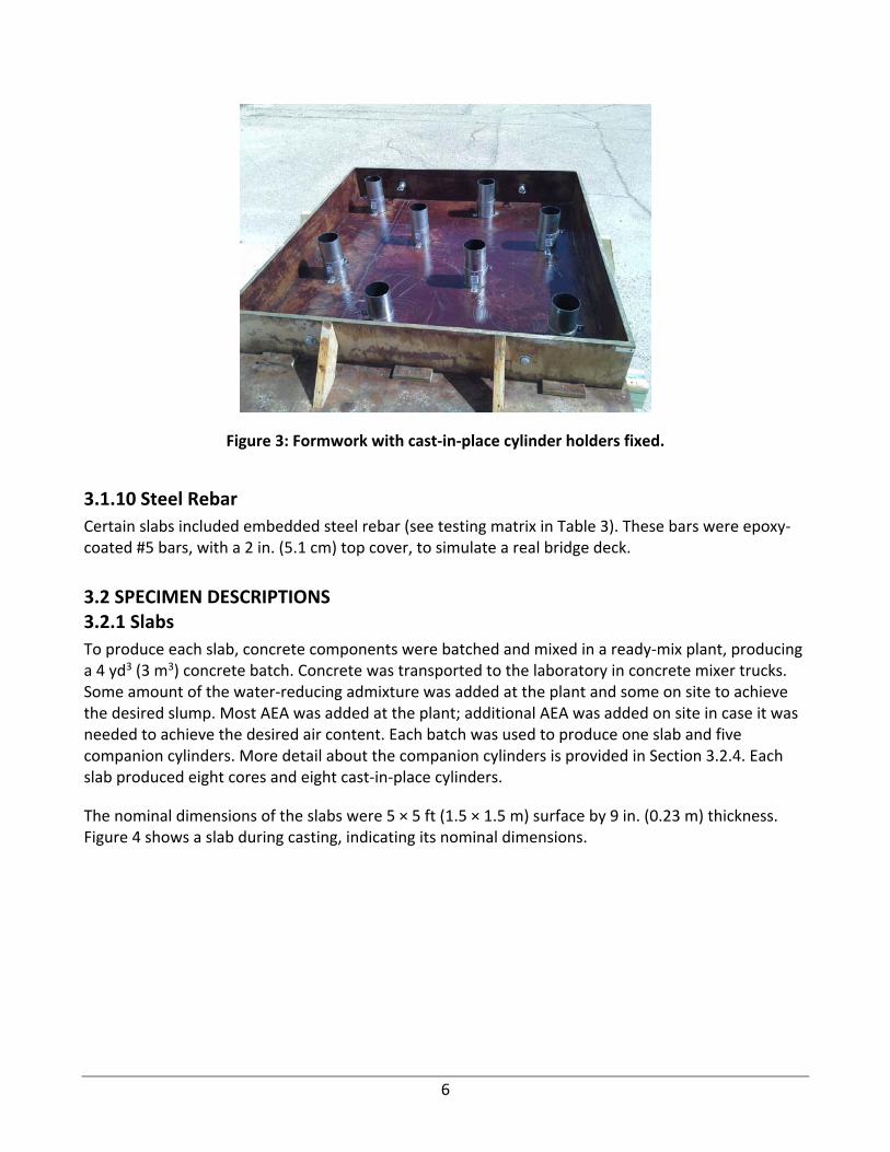
Each of these holders was assembled using one galvanized steel bracer, one galvanized steel sleeve, one foam pad disc, and one 4 × 8 plastic mold. The procedure to prepare holders was as follows: Each bracer was initially fixed to the form floor (plywood formwork of the slab) using screws. The foam pad was then put inside the sleeve, toward one of the ends. Next, the sleeve was set into the bracer, with the foam pad disc in contact with the form floor; the bracer was tightened to hold the sleeve firmly but without deforming it. The inner face of the sleeve was greased using form oil. Then the plastic mold was slid into the sleeve. If every piece of the cast in‐place cylinder holder was prepared and assembled correctly, the total height of the holder would be 9 in. (22.9 cm), with the plastic mold and sleeve top edges level. In addition, there would remain a gap of around 0.08 in. (2 mm) between the plastic mold and the sleeve; the top part of that gap was covered with Vaseline to prevent concrete seeping in during casting.
Figure 2 depicts the three main elements of the in‐place holder. The foam pad is not seen because it was placed inside the sleeve in contact with the form surface and below the plastic mold. Figure 3 shows the geometric configuration of the eight in‐place holders attached to the formwork.
Figure 2: In‐place cylinder holder.
6
Figure 3: Formwork with cast‐in‐place cylinder holders fixed.
3.1.10 Steel Rebar
Certain slabs included embedded steel rebar (see testing matrix in Table 3). These bars were epoxy‐coated #5 bars, with a 2 in. (5.1 cm) top cover, to simulate a real bridge deck.
3.2 SPECIMEN DESCRIPTIONS 3.2.1 Slabs
To produce each slab, concrete components were batched and mixed in a ready‐mix plant, producing a 4 yd3 (3 m3) concrete batch. Concrete was transported to the laboratory in concrete mixer trucks. Some amount of the water‐reducing admixture was added at the plant and some on site to achieve the desired slump. Most AEA was added at the plant; additional AEA was added on site in case it was needed to achieve the desired air content. Each batch was used to produce one slab and five companion cylinders. More detail about the companion cylinders is provided in Section 3.2.4. Each slab produced eight cores and eight cast‐in‐place cylinders.
The nominal dimensions of the slabs were 5 × 5 ft (1.5 × 1.5 m) surface by 9 in. (0.23 m) thickness. Figure 4 shows a slab during casting, indicating its nominal dimensions.

7
Figure 4: Slab dimensions.
Table 3 presents the experimental testing matrix, describing the main testing features of each slab.
Table 3: Experimental Testing Matrix
Slab Name Mixture
Core Treatment Rebar?
R1 PV/SI 1‐day dry No
R2 PV/SI 1‐day dry No
R3 PV/SI 1‐day wet No
R4 PV/SI 1‐day wet No
R5 PV/SI 1‐day dry Yes, inner*
R6 PV/SI 1‐day dry Yes, inner*
R7 PV/SI 1‐day dry Yes, outer**
R8 PV/SI 1‐day dry Yes, outer**
R9 PS 1‐day dry No
R10 PS 1‐day dry No
R11 PS 1‐day wet No
R12 PS 1‐day wet No
R13 PV/SI‐low 1‐day dry No
R14 PV/SI‐low 1‐day dry No
R15A PV/SI‐low 1‐day wet No
R16 PV/SI‐low 1‐day wet No
R15B PV/SI‐low 1‐day wet No
* Inner means that the rebar passed through the inner one‐third (area‐based computation) of the core.
** Outer means that the rebar passed through the outer two‐thirds (area‐based computation) of the core.
8
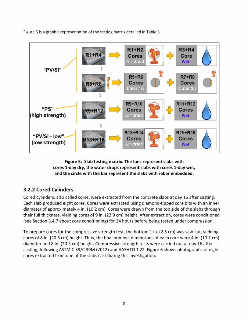
Figure 5 is a graphic representation of the testing matrix detailed in Table 3.
Figure 5: Slab testing matrix. The fans represent slabs with cores 1‐day dry, the water drops represent slabs with cores 1‐day wet, and the circle with the bar represent the slabs with rebar embedded.
3.2.2 Cored Cylinders
Cored cylinders, also called cores, were extracted from the concrete slabs at day 15 after casting. Each slab produced eight cores. Cores were extracted using diamond‐tipped core bits with an inner diameter of approximately 4 in. (10.2 cm). Cores were drawn from the top side of the slabs through their full thickness, yielding cores of 9 in. (22.9 cm) height. After extraction, cores were conditioned (see Section 3.4.7 about core conditioning) for 24 hours before being tested under compression.
To prepare cores for the compressive strength test, the bottom 1 in. (2.5 cm) was saw‐cut, yielding cores of 8 in. (20.3 cm) height. Thus, the final nominal dimensions of each core were 4 in. (10.2 cm) diameter and 8 in. (20.3 cm) height. Compressive strength tests were carried out at day 16 after casting, following ASTM C 39/C 39M (2012) and AASHTO T 22. Figure 6 shows photographs of eight cores extracted from one of the slabs cast during this investigation.

9
Figure 6: Picture of eight cores extracted from one of the slabs.
3.2.3 In‐Place Cylinders
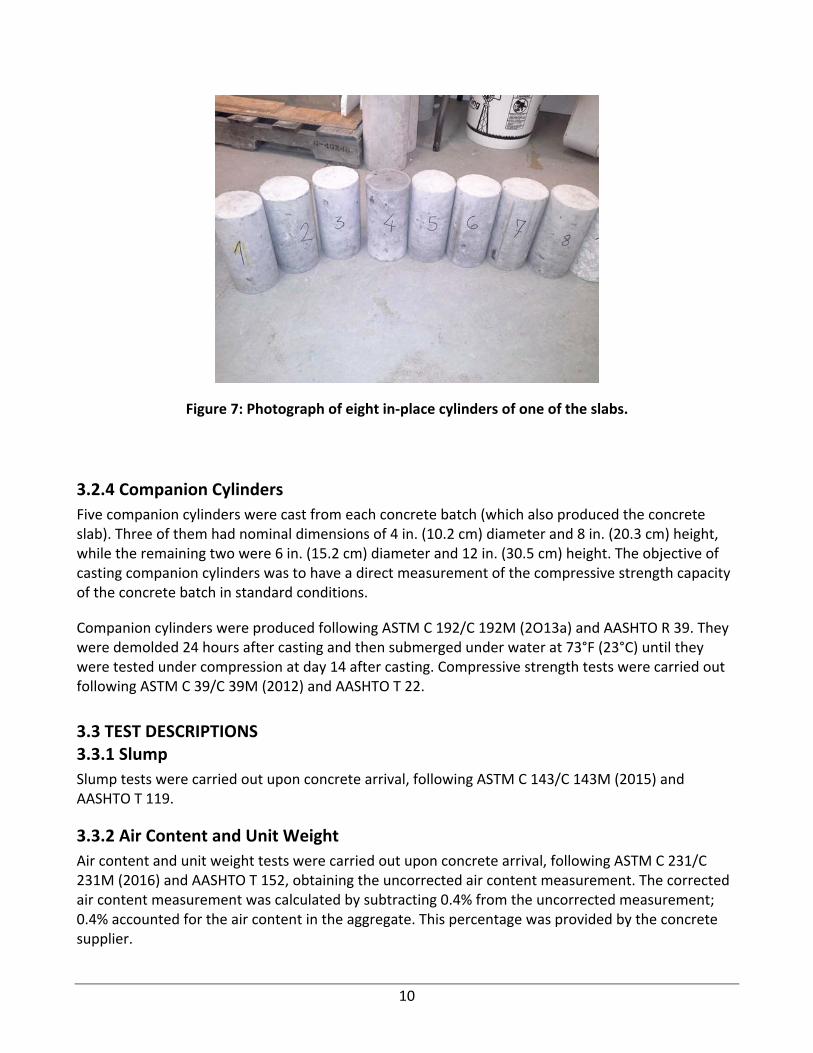
In‐place cylinders are also referred to as cast‐in‐place cylinders. Before each concrete slab was cast, eight in‐place cylinder holders were fixed to the bottom of the plywood formwork. The in‐place cylinders were cast by filling the molds in two layers and rodding (and tapping) each layer, as specified in ASTM C 192/C 192M (2013a) and AASHTO R 39; this was done immediately before pouring the concrete into the rest of the form to produce the slab. The research team carried out a side study to confirm that the consolidation of the in‐place cylinders using the rodding procedure yielded equivalently consolidated concrete as the rest of the slab. Details of that study are provided in Appendix C. In‐place cylinders were removed from the slab by pushing them from the bottom on day 16 after casting. Their final nominal dimensions were 4 in. (10.2 cm) diameter and 8 in. (20.3 cm) height. In‐place cylinders were tested under compression the same day of extraction. Compressive strength tests were carried out following ASTM C 39/C 39M (2012) and AASHTO T 22. Figure 7 shows photographs of eight in‐place cylinders of one of the slabs cast during this investigation.
10
Figure 7: Photograph of eight in‐place cylinders of one of the slabs.
3.2.4 Companion Cylinders
Five companion cylinders were cast from each concrete batch (which also produced the concrete slab). Three of them had nominal dimensions of 4 in. (10.2 cm) diameter and 8 in. (20.3 cm) height, while the remaining two were 6 in. (15.2 cm) diameter and 12 in. (30.5 cm) height. The objective of casting companion cylinders was to have a direct measurement of the compressive strength capacity of the concrete batch in standard conditions.
Companion cylinders were produced following ASTM C 192/C 192M (2O13a) and AASHTO R 39. They were demolded 24 hours after casting and then submerged under water at 73°F (23°C) until they were tested under compression at day 14 after casting. Compressive strength tests were carried out following ASTM C 39/C 39M (2012) and AASHTO T 22.
3.3 TEST DESCRIPTIONS 3.3.1 Slump
Slump tests were carried out upon concrete arrival, following ASTM C 143/C 143M (2015) and AASHTO T 119.
3.3.2 Air Content and Unit Weight
Air content and unit weight tests were carried out upon concrete arrival, following ASTM C 231/C 231M (2016) and AASHTO T 152, obtaining the uncorrected air content measurement. The corrected air content measurement was calculated by subtracting 0.4% from the uncorrected measurement; 0.4% accounted for the air content in the aggregate. This percentage was provided by the concrete supplier.

11
3.3.3 Compressive Strength
Compressive strength tests were carried out following ASTM C 39/C 39M (2012) and AASHTO T 22. In the cases of cores and in‐place cylinders, special attention was paid to obtain flat end faces (i.e., to the perpendicularity of the end faces with regard to the lateral face; some faces were saw‐cut to reach the correct level of perpendicularity required by IDOT3).
All compressive strength tests were carried out using steel caps with 60 durometer neoprene pads.
3.3.4 Longitudinal Dynamic Modulus
Longitudinal dynamic modulus tests (resonance tests) were carried out on cores and in‐place cylinders to obtain their longitudinal dynamic moduli. These tests were performed following ASTM C 215 (2002a). The dynamic moduli data were used as an additional parameter to monitor material mechanical properties.
Longitudinal dynamic moduli were obtained from cores and in‐place cylinders. Special care was taken to maintain the moisture condition of the samples throughout the testing period. Three resonance signals were obtained from each sample by measuring acceleration amplitude in time, following ASTM C 215 guidelines (2002a). The sampling rate was set at 1 MHz, yielding a time interval of 1 µs. Each signal was composed of 100,000 data points. From each signal, the longitudinal fundamental frequency was selected by carrying out a fast Fourier transform to obtain the amplitude spectrum in the frequency domain of the signal. For each sample, the three resonant frequencies were averaged and, from that average, the longitudinal dynamic modulus of the sample was computed.
3.3.5 Rebound Hammer
Slabs were tested using the Proceq N‐34 159279 (provided by the manufacturer, Proceq) rebound hammer equipment in vertical position, at eight testing locations. Ten replicates were collected at each testing location, with each replicate collected at least 1 in. (2.5 cm) away from the others, as specified in ASTM C 805 (2002b). Figure 8 is a picture of the rebound hammer employed in this investigation.
Figure 8: Photograph of the rebound hammer.
3 ASTM C 39/C39M (2012) and AASHTO T 22 indicate that “neither end of test specimens shall depart from perpendicularity to the axis by more than 0.5° (approximately equivalent to 1 mm in 100 mm),” which is extremely restrictive. Upon consultation with the Technical Review Panel for this project, the research team was informed that up to a 3 mm departure from perpendicularity would be allowed. This was permitted because the Technical Review Panel suspected the perpendicularity is not always followed in the field.
12
3.3.6 Nitto Hammer
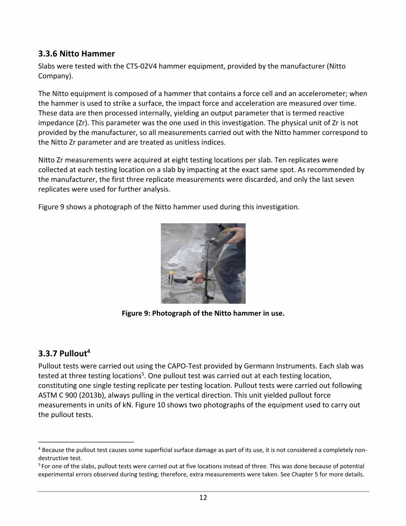
Slabs were tested with the CTS‐02V4 hammer equipment, provided by the manufacturer (Nitto Company).
The Nitto equipment is composed of a hammer that contains a force cell and an accelerometer; when the hammer is used to strike a surface, the impact force and acceleration are measured over time. These data are then processed internally, yielding an output parameter that is termed reactive impedance (Zr). This parameter was the one used in this investigation. The physical unit of Zr is not provided by the manufacturer, so all measurements carried out with the Nitto hammer correspond to the Nitto Zr parameter and are treated as unitless indices.
Nitto Zr measurements were acquired at eight testing locations per slab. Ten replicates were collected at each testing location on a slab by impacting at the exact same spot. As recommended by the manufacturer, the first three replicate measurements were discarded, and only the last seven replicates were used for further analysis.
Figure 9 shows a photograph of the Nitto hammer used during this investigation.
Figure 9: Photograph of the Nitto hammer in use.
3.3.7 Pullout4
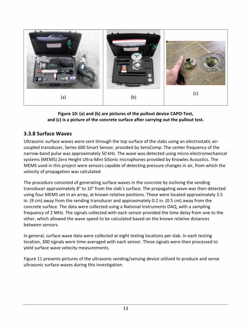
Pullout tests were carried out using the CAPO‐Test provided by Germann Instruments. Each slab was tested at three testing locations5. One pullout test was carried out at each testing location, constituting one single testing replicate per testing location. Pullout tests were carried out following ASTM C 900 (2013b), always pulling in the vertical direction. This unit yielded pullout force measurements in units of kN. Figure 10 shows two photographs of the equipment used to carry out the pullout tests.
4 Because the pullout test causes some superficial surface damage as part of its use, it is not considered a completely non‐destructive test. 5 For one of the slabs, pullout tests were carried out at five locations instead of three. This was done because of potential experimental errors observed during testing; therefore, extra measurements were taken. See Chapter 5 for more details.
13
(a)
(b)
(c)
Figure 10: (a) and (b) are pictures of the pullout device CAPO‐Test, and (c) is a picture of the concrete surface after carrying out the pullout test.
3.3.8 Surface Waves
Ultrasonic surface waves were sent through the top surface of the slabs using an electrostatic air‐coupled transducer, Series 600 Smart Sensor, provided by SensComp. The center frequency of the narrow‐band pulse was approximately 50 kHz. The wave was detected using micro‐electromechanical systems (MEMS) Zero Height Ultra‐Mini SiSonic microphones provided by Knowles Acoustics. The MEMS used in this project were sensors capable of detecting pressure changes in air, from which the velocity of propagation was calculated.
The procedure consisted of generating surface waves in the concrete by inclining the sending transducer approximately 8° to 10° from the slab’s surface. The propagating wave was then detected using four MEMS set in an array, at known relative positions. These were located approximately 3.5 in. (9 cm) away from the sending transducer and approximately 0.2 in. (0.5 cm) away from the concrete surface. The data were collected using a National Instruments DAQ, with a sampling frequency of 2 MHz. The signals collected with each sensor provided the time delay from one to the other, which allowed the wave speed to be calculated based on the known relative distances between sensors.
In general, surface wave data were collected at eight testing locations per slab. In each testing location, 300 signals were time‐averaged with each sensor. These signals were then processed to yield surface wave velocity measurements.
Figure 11 presents pictures of the ultrasonic sending/sensing device utilized to produce and sense ultrasonic surface waves during this investigation.

14
(a)
(b)
(c)
Figure 11: Photographs of the ultrasonic sending/sensing homemade device: (a) the frame holding the blue transducer set in position to test, (b) a bottom view the
sending transducer and receivers (MEMS), and (c) receiver array.
3.3.9 Temperature Monitoring
Temperature was monitored using the TC‐08 data logger, provided by Omega. Type‐K thermocouple wires were employed. Figure 12 shows a photograph of the TC‐08 data logger. Internal concrete temperatures were monitored to ensure that concrete within the in‐place cylinders and in the body of the slab experienced similar temperature histories.
Figure 12: Photograph of the TC‐08 data logger for temperature monitoring.
15
3.4 GENERAL CASTING PROCEDURE
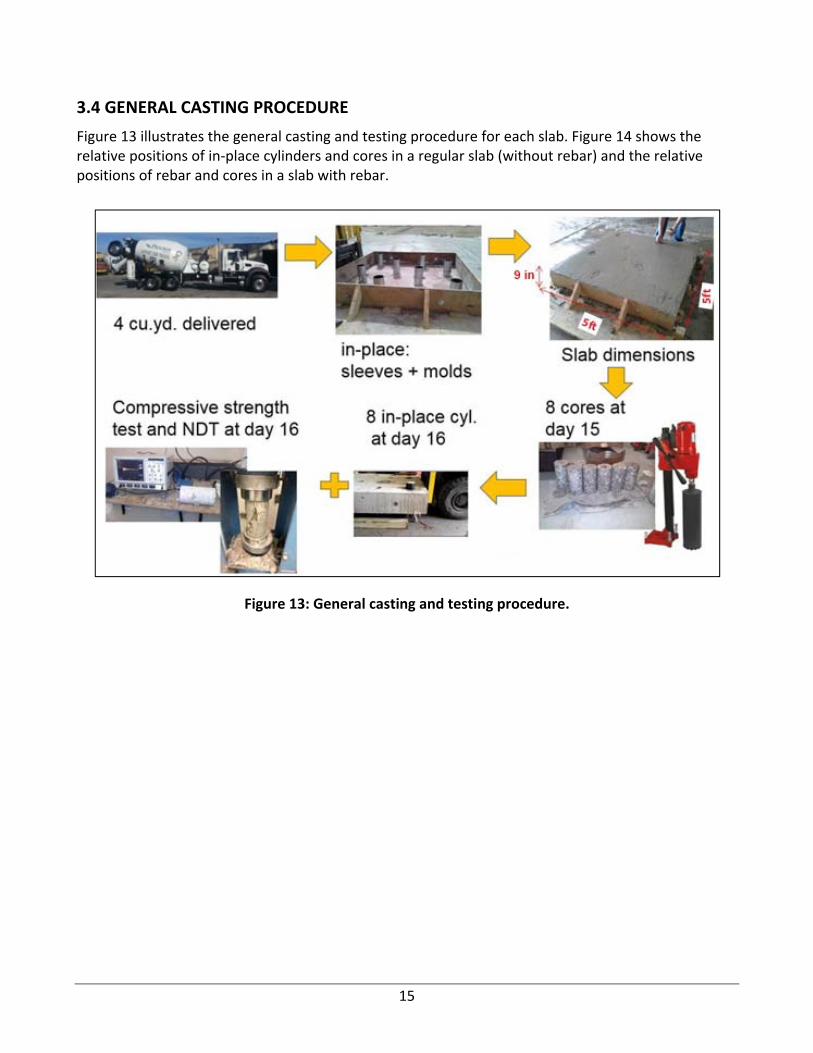
Figure 13 illustrates the general casting and testing procedure for each slab. Figure 14 shows the relative positions of in‐place cylinders and cores in a regular slab (without rebar) and the relative positions of rebar and cores in a slab with rebar.
Figure 13: General casting and testing procedure.

16
Figure 14: Plan view of a slab showing nominal relative positions between cores and in‐place cylinders, and between cores and embedded rebar. Inner one‐third rebar cores and outer two‐thirds cores were in separate slabs.
3.4.1 Step 1: Preparation
Preparation began with cleaning and assembling the formwork. Some slabs had embedded rebar; in those cases, the steel bars were set in position during this step.
On the pouring day, burlap bags were submerged in water. The clean formwork was set outdoors and leveled. Galvanized steel bracers were fixed in position. Galvanized steel sleeves had been previously constructed. Foam pad discs, sleeves, and plastic molds were set into the bracers following the description presented in Section 3.1.9, “In‐Place Cylinder Holder.”
A demolding agent (form oil) was sprayed on the inside of the form. The outside of the galvanized steel sleeve was wetted with water.
3.4.2 Step 2: Casting
Concrete was delivered by a concrete mixer truck. Slump, air content, and unit weight tests were carried out upon arrival to determine whether to accept or reject the batch. Occasionally, additional AEA and/or a water‐reducing admixture or high range water‐reducing admixture was added to increase the air content and/or the slump, respectively, to meet the requirements of the specific mixture design (see Table 1 for target properties).

17
Once the batch was accepted, the cast‐in‐place cylinders were cast first, following the procedure described in Section 3.2.3, “In‐Place Cylinders.” The rest of the concrete was then poured into the form. Immediately after the concrete was poured, the form (holding the fresh concrete) was moved indoors onto a leveled floor. There, the concrete was vibrated using the internal vibrator following recommended practice: the vibrating head was inserted vertically downward into the concrete at a rapid rate, but without touching the bottom of the form, and then more slowly lifted vertically to the surface (Mindess et al. 2003). After vibration, the screeding process was performed using a wood 2 × 4, followed by steel troweling to improve the finished surface.
Five companion cylinders were cast at the same time as the slab was being poured.
One thermocouple wire was inserted into one of the in‐place cylinders to monitor temperature at mid depth. Another thermocouple wire was inserted into the slab’s concrete (outside any in‐place cylinder) to monitor concrete temperature at mid depth. Air temperature was monitored using a third thermocouple wire. Temperature measurements were collected at a rate of one measurement every 30 seconds during at least 66 hours after casting.
3.4.3 Step 3: Curing Slab and Demolding Companion Cylinders
Curing was performed by wetting burlap and using plastic sheets to prevent evaporation. The slabs made of concrete mixtures PV/SI and PV/SI‐low were moist‐cured for 3 days, except for slab R15B, which was moist‐cured for 4 days6. The slabs made of the concrete mixture PS were moist‐cured for 1 day. Companion cylinders were demolded the day after casting and were immediately put in the water bath.
3.4.4 Step 4: Form Removal
Forms were removed from the concrete slabs no earlier than day 3 after casting.
3.4.5 Step 5: Companion Cylinder Tests
The five companion cylinders were tested under compression on day 14 after casting, following ASTM C 39/C 39M (2012) and AASHTO T 22. Measurements collected were visual inspection, height, diameter, roughness, perpendicularity, mass, maximum load, and type of break; these data are presented in Appendix A.
3.4.6 Step 6: Coring
Eight cores were extracted on day 15 after casting. To perform this task, the slabs were moved and leveled outdoors. A polystyrene sheet was placed below the slab to avoid damaging the cores by impacting the underlying pavement. Coring was carried out by positioning the core bit onto the slab and letting it fall downward by self‐weight as the drilling progressively advanced. The eight cores were then moved indoors for moisture conditioning.
6 Note that IDOT requires 7‐day moist curing for SI mixtures and 3‐day moist curing for PV mixtures.

18
3.4.7 Step 7: Core Conditioning
Two types of moisture conditioning were performed in this investigation: 1‐day wet (submerging the cores in a water bath) and 1‐day dry (placing the cores in front of a three‐speed fan with speed set to medium in the laboratory under uncontrolled room temperature and moisture conditions). Figure 15 depicts the configuration during the core’s air drying.
(a)
(b)
Figure 15: (a) geometric configuration of fan and cores used during the air‐drying conditioning (1‐day dry core conditioning), and (b) a photograph of the box fan used.
3.4.8 Step 8: Saw‐Cutting Cores
Because the slab thicknesses were 9 in. (22.9 cm), the bottom 1 in. (2.5 cm) of the cores were saw‐cut to obtain 4 in. (10.2 cm) diameter by 8 in. (20.3 cm) high cores. This task was carried out on day 16, before the other tests were carried out. If a core’s top surface happened to be out of perpendicu‐larity, a thin slice was saw‐cut from it to improve that characteristic. Perpendicularity measurements are presented in Appendix A.
3.4.9 Step 9: Extracting In‐Place Cylinders
In‐place cylinders were extracted on day 16 after casting. To perform this task, the slab was lifted up about 3 ft (1 m) from the floor using a truck lifter (Bobcat). A wood 2 × 2 was set in contact with the in‐place cylinder bottom and the floor. Then the slab was slowly moved down so that the plastic mold (containing the in‐place cylinder) would slide out from the galvanized steel sleeve (fixed to the rest of the slab) and thus be held up by the wood 2 x 2.
19
After the in‐place cylinders had been extracted, they were demolded and moved to the testing section of the laboratory. Some in‐place cylinders had an excess of concrete at their top end; this excess was either saw‐cut out or ground out to obtain the appropriate cylindrical dimensions.
3.4.10 Step 10: Cores and In‐Place Cylinder Testing
Cores and in‐place cylinders were tested on day 16 after casting. By that point, the cores had been conditioned for 24 hours and then saw‐cut; also, the in‐place cylinders had been extracted from the slab and then demolded.
The first measurement collected was perpendicularity. In the case of unacceptable perpendicularity (see Section 3.3.3, “Compressive Strength”), the cylinder was saw‐cut or grounded down to improve this property. Then the cylinders were weighed, and geometrical dimensions were measured as in accordance with ASTM C 39/C 39M (2012) and AASHTO T 22.
Special care was taken to maintain the cores’ moisture condition; thus, cores were kept either submerged or in front of the fan when they were not being measured.
Longitudinal dynamic elastic modulus tests were then carried out on cores and in‐place cylinders. Finally, cores and in‐place cylinders were tested under compression, following ASTM C 39/C 39M (2012) and AASHTO T 22, to obtain the failure force and type of breaking.
3.4.11 Step 11: NDT Testing in Slab
The undamaged parts of the slab were used to carry out the NDT. Eight testing locations were defined for each of the three NDT methods (rebound hammer, Nitto hammer and surface waves). Three testing locations were defined for carrying out the NDT pullout tests.

20
CHAPTER 4: ANALYTICAL PROCEDURES
4.1 DATA PROCESSING ASSOCIATED WITH THE EXPERIMENTS 4.1.1 Slump
No processing was done with the slump measurements.
4.1.2 Air Content and Unit Weight
The air content test yielded an uncorrected air content measurement. The corrected air content measurement was calculated by subtracting 0.4% from the uncorrected air content measurement, to account for the air content in the aggregate. This number was provided by the concrete supplier.
The unit weight measurement was obtained using a scale to measure the weight of the fresh concrete in the specified metal bucket of known volume. The unit weight was calculated by directly dividing the measured weight by the known volume.
4.1.3 Compressive Strength
The procedures described here were applied to all cylindrical test samples, including core, in‐place and companion samples. The compressive strength tests included several subtests to measure the sample’s roughness, perpendicularity, height, diameter, failure load, type of break, and final compressive strength. All these parameters were measured following ASTM C 39/C 39M (2012) and AASHTO T 22.
The perpendicularity of each edge face was estimated by setting a square at the angle formed by the cylinder’s edge face and lateral face, pressing the square firmly to the flat lateral side of the cylinder. The maximum air gap formed between the square and the edge face, measured at the diametrically opposed side of where the square was set, was considered to be the perpendicularity measurement.
The roughness of each edge face was measured by setting a ruler on each edge face and estimating the air gap distance between the uneven surface and the ruler. These measurements provided an estimation of the distance between peaks and valleys of the uneven concrete surface.
Three height measurements were taken using a caliper. Two diameter measurements were collected using a caliper—both at the cylinder’s mid height but on two diameters 90° from each other. In the case of the 6 × 12 companion cylinders, the caliper could not be used because of the large dimensions of the cylinders, so a metric tape was employed to measure height and a measuring clamp was employed to measure diameter.
The cross‐section area of each cylinder was computed from the average of the measured diameters.
The failure load was obtained from the compressive strength failure load. The type of break was based on visual inspection of the failed sample after the compressive strength test.
21
The compressive strength of each cylinder was computed by dividing the failure load by the cross‐sectional area.
4.1.4 Longitudinal Dynamic Modulus
The sample’s longitudinal dynamic modulus was obtained by analyzing the collected signals as specified in ASTM C 215 (2002a). The longitudinal fundamental frequency of vibration was obtained from each sample by performing a fast Fourier transform of time‐domain signals. Three time‐domain signals per sample were processed in this way, and the average of the three frequencies composed the final fundamental frequency of the sample.
Once the fundamental frequency was computed, the longitudinal dynamic modulus El, d, in units of Pascals, was calculated as follows:
, 5.093 (Equation 1)
where L is the cylinder’s length in meters, d is the diameter in meters, M is the mass in kilograms, and f is the longitudinal fundamental frequency of vibration in Hertz.
4.1.5 Rebound Hammer
The data collected with the rebound hammer were processed as specified in ASTM C 805 (2002b).
As explained in Section 3.3.5, in general, each slab was tested with the rebound hammer at eight testing locations, and ten measurement repetitions were collected at each testing location. Each repetition was therefore one real reading given by the apparatus in a specific test, with each of the readings taken from a different physical spot, at least 1 in. (2.5 cm) away from the others. The first processing of that set was to take the mean (average) of those ten measurements; then, if any one of the ten measurements was six units or more away from the mean, that particular measurement was discarded, and a new mean was calculated from the remaining nine measurements. If any one of the nine remaining measurements was six units or more away from the new calculated mean, the entire set was discarded.
To summarize, the final outputs of rebound hammer tests were, for each slab, eight rebound numbers, collected from eight locations of the slab. These eight rebound numbers were the only ones that were further analyzed and discussed for each slab.
4.1.6 Nitto Hammer
The data collected with the Nitto hammer were processed as recommended by the manufacturer.
As explained in Section 3.3.6, each slab was tested with the Nitto hammer at eight testing locations, and ten measurement repetitions were collected at each testing location. Each of these repetitions was a reactive impedance (Zr) reading given by the equipment. Within testing locations, all ten measurement repetitions were collected by striking the hammer at the exact same spot. Then the first three repetitions were discarded from the set, and the last seven repetitions were averaged to compute the final average of the set.

22
Therefore, the final outputs of Nitto hammer tests were, for each slab, eight Zr, collected from eight locations of the slab. These sets of eight Zr were the only ones that were further analyzed and discussed
4.1.7 Pullout
As explained in Section 3.3.7, each slab was tested at three testing locations (in this case, one testing location corresponds to one testing replicate). These three pullout measurements of each slab were used for further analysis and discussion.
4.1.8 Surface Waves
As explained in Section 3.3.8, each slab was tested at eight testing locations by collecting ultrasonic surface wave signals using a sending transducer and four sensors.
At each of these locations, four time‐domain signals were collected, each signal associated with one sensor. At each testing location, it was possible to obtain the relative time delay of the wave arrival between signals (between sensors). Because the relative distances between sensors was known, it was possible to calculate the velocity of wave propagation by fitting a linear trend between the relative time delays and the relative distances between sensors; the slope of that best‐fit line was used as the surface wave velocity.
4.1.9 Temperature Monitoring
No additional processing was carried out with the temperature data.
4.2 USE OF BOXPLOTS
Boxplots are used to graphically show the statistical variation of a dataset. As it can be seen in Figure 16, the boxplot scheme is composed of two horizontal lines indicating the maximum and minimum values of the dataset; a box, whose edges indicate the 75th and 25th percentiles of the dataset; and another horizontal line inside the box, which indicates the median. In addition, crosses indicate the outliers of the dataset. Unless otherwise specified, throughout this report, the criterion to define a certain data value as a statistical outlier was as follows: if a data point was at least 2.7 times the standard deviation of the dataset away from the median, that point was considered an outlier. It should be noted that other data points could have been discarded for other reasons. Every time a data value was discarded, the justification for doing is explicitly provided in this report (see Chapter 5).

23
Figure 16: Explanation of boxplot.
4.3 STATISTICAL ANALYSIS
Analysis of variance (ANOVA) is used to evaluate whether groups of strength data are statistically
equivalent. This approach is an extension of the two‐sample t‐test for means assuming normally
distributed datasets but unequal variance among the compared populations. Hypotheses are often
employed in statistical analysis to express results. In this study, we assumed the following null
hypothesis: “Population samples for a particular type of core condition or from an NDT test have the
same mean value as that from the molded in‐place cylinder samples for a given concrete mixture and
condition.” The alternative hypothesis is then “Population samples have different mean values.” In
this study, the hypothesis analysis was carried out at a 95% confidence level, meaning only a 5%
chance of a false positive reading. If the null hypothesis was rejected, then the alternative hypothesis
was accepted and we stated, with a 95% confidence level, that the population sets had different
mean values; in that case, we developed a correlation between the strength values. If the null
hypothesis was not rejected, then we stated that the mean values of the population sets were not
significantly different, with 95% confidence. These analyses were carried out separately for each
material type and test case.
Figure 17 describes the procedure to obtain the possible correction factors associated with the compared populations for slab R3. Core strength multiplied by different correction factors (shown at top of graph) and populations were compared to determine whether they were statistically different, under certain assumptions. Orange circles represent the compressive strengths of the cores multiplied by the corresponding correction factor, and blue circles represent the compressive strengths of the in‐place cylinders (“InCyl”). The word “different” is used to designate populations

24
that were statistically different at a 95% confidence level. When two populations that each contained eight cylinders were compared, the parameter limit F was 4.6 for 95% confidence. By applying different correction factors to the core data and then comparing them with the in‐place strengths, we see that the optimal correction factor (F‐score is equal to zero) for this particular dataset is near the value of 1.15. The 95% confidence range of correction factors and the optimal correction factor for each slab are computed and discussed in Section 5.9.1 of this report.
Figure 17: Example of correction factor calculation (slab R3) using ANOVA analysis.
4.4 RANDOM SAMPLING ANALYSIS
Random sampling analysis studies how the error between measured and estimated strengths is reduced when additional strength estimates are considered. The strength estimates are obtained from an indirect measurement to which a certain correlation curve or correction factor is applied. These indirect measurements could be core strength measurements or NDT measurements.
Results from cores and each NDT method were studied individually. To explain the analysis, consider strength estimation method from core samples obtained from one particular slab. Several cores were drawn from the slab and tested (or several testing locations for the case of NDT methods) yielding several core strength values. One can randomly select one of those core strength values and transform it to an estimated strength using the corresponding correction factor (or OLS correlation curve for the case of the NDT methods) already calculated. Then the difference between the measured strength and estimated strength can be quantified with the absolute error (Abs.Err):

25
. % 100| |
(Equation 2)
where Yest corresponds to the strength estimated using the core strength and Ymeas is the measured strength using the in‐place cylinders (average of eight cylinders per slab).
The use of the absolute value of the strength estimate errors gives an idea of how off the strength
predictions are from the real strength, but it does not differentiate which “side” the error is located. In
other words, using the absolute value does not indicate if the prediction overestimates (non‐
conservative estimate) or underestimates (conservative estimate) the actual in‐place strength.
To study the statistical behavior of the absolute error values, every possible core strength result was considered, one at a time, and one absolute error value was calculated from each of them using Equation 2. The obtained dataset corresponds to absolute strength error associated with considering one core strength value at a time (i.e., # Cores = 1).
One can expect that if two cores are tested and averaged, the resulting estimated strength would yield a lower expected error than when estimating the strength from a single core. The analysis thus continued by calculating all possible combinations of core strength values, taking them in pairs; each pair was averaged, yielding as many Yest as there were possible combinations of core strength values. Then the strength absolute errors were calculated from the new Yest data (associated with # Cores = 2). This new dataset corresponded to strength absolute errors associated with # Cores = 2. This procedure was further carried out by considering all possible combinations of three core strength values, successively up to Nloc, where Nloc is the total number of core values for a specific slab.
Then the Abs.Err. values were calculated for each slab and aggregated to form a different data population for each of the # Cores. One histogram was constructed for each of the datasets associated with each # Cores. The metric named Abs.Err95 was computed for each histogram (each histogram associated with each # NDT locations for every NDT method). The metric Abs.Err95 corresponded to the absolute error of the histogram that leaves 95% of those errors below it and 5% higher; in other words, Abs.Err95 corresponds to the 95th percentile of the population at each histogram. In an analogous procedure, the metrics Abs.Err85 and Abs.Err75 were also computed.
The same analysis applies for the three NDT methods by substituting # Cores with “# NDT locations, and noting that the strength estimates come from the application of a certain correlation curve instead of a single correction factor. Also, for the NDT cases, Nloc = 8 for rebound hammer and Nitto hammer, and Nloc = 3 for pullout.
The random sampling analysis allows obtaining the expected strength error curves which show how the expected error of the strength prediction varies with increasing number of tested cores (or NDT locations). For the case of the cores, the expected strength error curves are plotted at three different confidence percentiles: 75%, 85%, and 95%. For the NDT cases, only the 95% confidence percentile is carried out, but using three different correlation curves.
Particularly for the core’s random sampling analysis, an additional analytical approach was carried out using the aggregated data of strength errors previously mentioned. In this case, instead of prescribing
26
a fixed confidence percentile and observing how the expected strength error drops with increasing number of cores, the expected strength error is now prescribed and the confidence is then calculated. The expected strength error was defined as 5%, and confidence of the estimation was computed by calculated the percentage of strength estimations that have an error lower than 5%. As more cores are considered to compute the strength estimation, the confidence of having a 5% error or lower increases.
An example of the application of random sampling analysis is presented in Appendix D which provides more detail and explanation for the reader.
4.5 ANALYSIS OF NDT VS. IN‐PLACE CYLINDER COMPRESSIVE STRENGTH
This analysis studied the correlation of NDT carried out on the concrete slabs vs. the compressive strength of in‐place cylinders.
4.5.1 NDT vs. Compressive Strength Relationships
Four sets of data were obtained from each slab. The first dataset corresponded to the averaged values of in‐place cylinders (i.e., one strength value per slab, each being the average of the eight cylinders). The other three datasets corresponded to NDT location values of rebound hammer, Nitto hammer, and pullout tests, respectively.
NDT vs. strength relationships (correlation curves) were calculated using the described datasets by following the specifications given in ACI 228.1R (2003). For each NDT method, two regression methods were computed to obtain two types of correlation curves. These were the ordinary least squares method (OLS) and the natural logarithm ordinary least squares method (logOLS). The OLS method is a linear approximation, whereas the logOLS method is a power approximation.
Therefore, the application of the OLS method yields an equation that correlates NDT values to strength values as
(Equation 3)
where X is an NDT value, Y is an estimated strength value, and a and b are the slope and Y‐intercept of the correlation curve, respectively. In the case of the logOLS method, the correlating equation is
(Equation 4)
where A and B are the parameters characteristic of the logOLS fit.
4.5.2 NDT Variability
The variability of the NDT results is composed of two variability sources. One corresponds to the inherent variability of the NDT method, and the other to the variability of the structure’s material (i.e., the slab’s concrete). These types of variability were analyzed together and are generically called NDT variability. The NDT variability was assessed by taking the range of NDT location results in each
27
slab. Non‐destructive testing variability at each slab was graphically represented either with a boxplot, as shown in Figure 36, Figure 37, and Figure 38, or with horizontal error bars, as shown in Figure 39. To quantify the NDT variability across all slabs, the metric average range (Avg.Range) was calculated as
.∑
(Equation 5)
where Rangei corresponds to the range of the NDT location values of slab i, and N is the total number of slabs tested.
4.5.3 Correlation Curve Uncertainty
The residual standard deviation (RSD) is a parameter that ACI 228.1R (2003) proposes for quantifying the uncertainty of a linear regression analysis. The RSD was estimated as
(Equation 6)
where N is the total number of slabs, Yi is the computed strengths of each slab (average of eight compressive strength values in general), Xi is the NDT average values of each slab, and f(Xi) is estimated strength values computed by applying the corresponding correlation curve to the Xi values. In other words, the values Yi ‐ f(Xi) correspond to the deviations from the measured average strengths and estimated average strengths of slab i.
4.5.4 NDT Sensitivity
The sensitivity of an NDT method is a metric that characterizes its ability to predict strength. More sensitive methods are able to distinguish between concretes with closer strength values. One way to quantify sensitivity is to use the slope of a linear best‐fit line. In this report, the slope of the ordinary least OLS best‐fit line was employed to evaluate sensitivity. In the case of non‐linear trend lines, their range of slopes could be used to assess sensitivity.
A NDT vs. strength relationship with lower slope indicates higher sensitivity of the NDT method, where the NDT data are the independent variable (horizontal axis) and the estimated strength is the dependent variable (vertical axis).
4.5.5 NDT Random Sampling Analysis
The random sampling analysis uses the NDT and strength data to compute the expected errors that occur as a result of using NDT for strength prediction. The analytical procedure was carried out as explained in Section 4.4.
2
)(1
2
N
XfYRSD
N
iii

28
CHAPTER 5: RESULTS AND DISCUSSION
5.1 OUTLIERS OR EXCLUDED DATA
Before presenting the results, it should be noted that the testing matrix included two slabs designated R15: R15A, which was cast first; and R15B. The cores and in‐place cylinders of R15A were drawn from the slab 1 day earlier than they should have been owing to a scheduling miscommunication with the assigned technician. Therefore, it was decided to cast a replicate of R15 and not to analyze R15A. However, the NDT of R15A was carried out normally, so it was decided to include those results in the NDT analysis.
The following is a summary of specific missing and excluded data:
The value of mass of the in‐place cylinder identified as InCyl_1 from slab R7 is significantly higher than the rest, yielding a density value statistically different from the rest of the set. As a result, the dynamic modulus result would also be flawed, so it was also excluded from the analysis.
The 4 × 8 companion cylinder identified as Comp_3 of slab R2 was not tested under compression because it the mold deformed during curing so the cylinder had an ellipsoidal cross‐section instead of circular.
The 6 × 12 companion cylinder identified as Comp_4 of slab R4 suffered damage during transportation, so it was not tested under compression.
The compressive strength of the core identified as Core_6, the in‐place cylinder InCyl_4, and the in‐place cylinder InCyl_6 (all from slab R10) could not be recorded because the loading machine had an electrical problem during testing.
The exclusion of these limited data are not expected to have any significant effect on the analysis of the remaining data. The results of slab R7 showed unusual and different trends from the rest of the slabs. Section 5.8 is a specific analysis of R7; it was decided to reject those results and exclude them from the rest of the discussion and analysis.
5.2 FRESH CONCRETE PROPERTIES AND TEMPERATURE MONITORING 5.2.1 Fresh Concrete Properties
Table 4contains the fresh concrete experimental results of all slabs. Other fresh concrete experimental data can be found in Table A.1 and Table A.2 in Appendix A. The fresh concrete properties included in Table 4 were employed to accept or reject the delivered concrete at the moment of casting. No additional analyses were carried out using the fresh concrete properties.
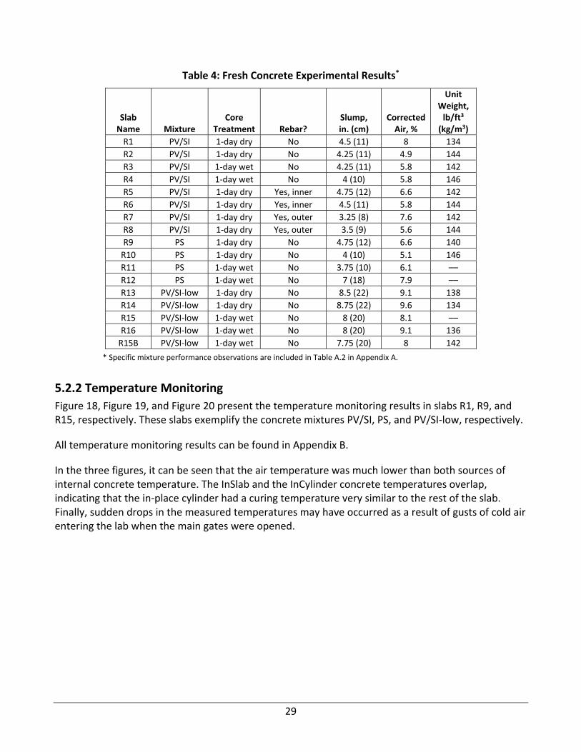
29
Table 4: Fresh Concrete Experimental Results*
Slab Name Mixture
Core Treatment Rebar?
Slump, in. (cm)
Corrected Air, %
Unit Weight, lb/ft3 (kg/m3)
R1 PV/SI 1‐day dry No 4.5 (11) 8 134
R2 PV/SI 1‐day dry No 4.25 (11) 4.9 144
R3 PV/SI 1‐day wet No 4.25 (11) 5.8 142
R4 PV/SI 1‐day wet No 4 (10) 5.8 146
R5 PV/SI 1‐day dry Yes, inner 4.75 (12) 6.6 142
R6 PV/SI 1‐day dry Yes, inner 4.5 (11) 5.8 144
R7 PV/SI 1‐day dry Yes, outer 3.25 (8) 7.6 142
R8 PV/SI 1‐day dry Yes, outer 3.5 (9) 5.6 144
R9 PS 1‐day dry No 4.75 (12) 6.6 140
R10 PS 1‐day dry No 4 (10) 5.1 146
R11 PS 1‐day wet No 3.75 (10) 6.1 ––
R12 PS 1‐day wet No 7 (18) 7.9 ––
R13 PV/SI‐low 1‐day dry No 8.5 (22) 9.1 138
R14 PV/SI‐low 1‐day dry No 8.75 (22) 9.6 134
R15 PV/SI‐low 1‐day wet No 8 (20) 8.1 ––
R16 PV/SI‐low 1‐day wet No 8 (20) 9.1 136
R15B PV/SI‐low 1‐day wet No 7.75 (20) 8 142
* Specific mixture performance observations are included in Table A.2 in Appendix A.
5.2.2 Temperature Monitoring
Figure 18, Figure 19, and Figure 20 present the temperature monitoring results in slabs R1, R9, and R15, respectively. These slabs exemplify the concrete mixtures PV/SI, PS, and PV/SI‐low, respectively.
All temperature monitoring results can be found in Appendix B.
In the three figures, it can be seen that the air temperature was much lower than both sources of internal concrete temperature. The InSlab and the InCylinder concrete temperatures overlap, indicating that the in‐place cylinder had a curing temperature very similar to the rest of the slab. Finally, sudden drops in the measured temperatures may have occurred as a result of gusts of cold air entering the lab when the main gates were opened.

30
Figure18: Temperature monitoring of slab R1. “Air” corresponds to air temperature measurements close to the slab. “InSlab” corresponds to temperature measurements collected
by a thermocouple inserted in the slab concrete outside any in‐place cylinder at mid depth. “InCyl” corresponds to a thermocouple inserted into an in‐place cylinder at mid depth.
Figure 19: Temperature monitoring of slab R9. “Air” corresponds to air temperature measurements close to the slab. “InSlab” corresponds to temperature measurements collected by a thermocouple inserted in the slab concrete outside any in‐place cylinder at mid depth. “InCyl”
corresponds to a thermocouple inserted into an in‐place cylinder at mid depth.

31
Figure 20: Temperature monitoring of slab R13. “Air” corresponds to air temperature measurements close to the slab. “InSlab” corresponds to temperature measurements collected by a thermocouple inserted in the slab concrete outside any in‐place cylinder at mid depth. “InCyl”
corresponds to a thermocouple inserted into an in‐place cylinder at mid depth.
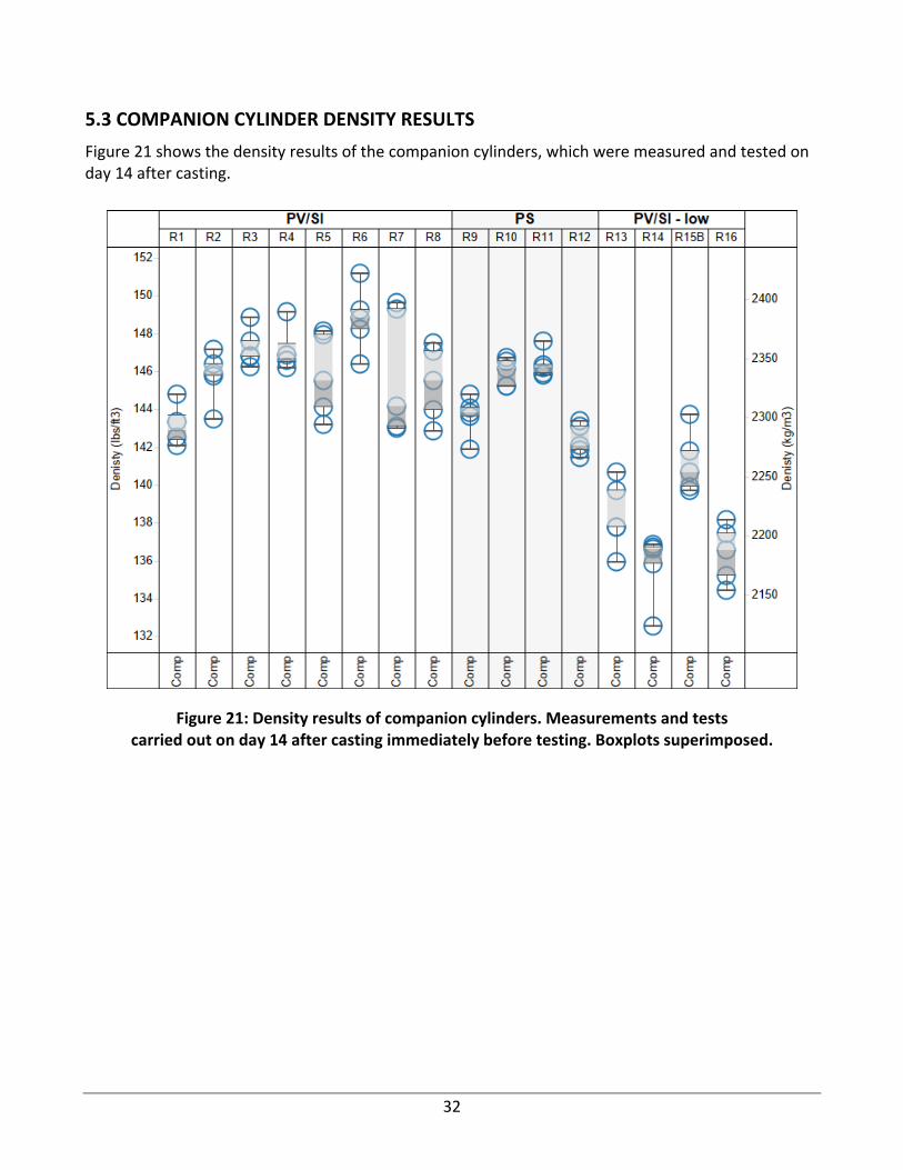
32
5.3 COMPANION CYLINDER DENSITY RESULTS
Figure 21 shows the density results of the companion cylinders, which were measured and tested on day 14 after casting.
Figure 21: Density results of companion cylinders. Measurements and tests carried out on day 14 after casting immediately before testing. Boxplots superimposed.
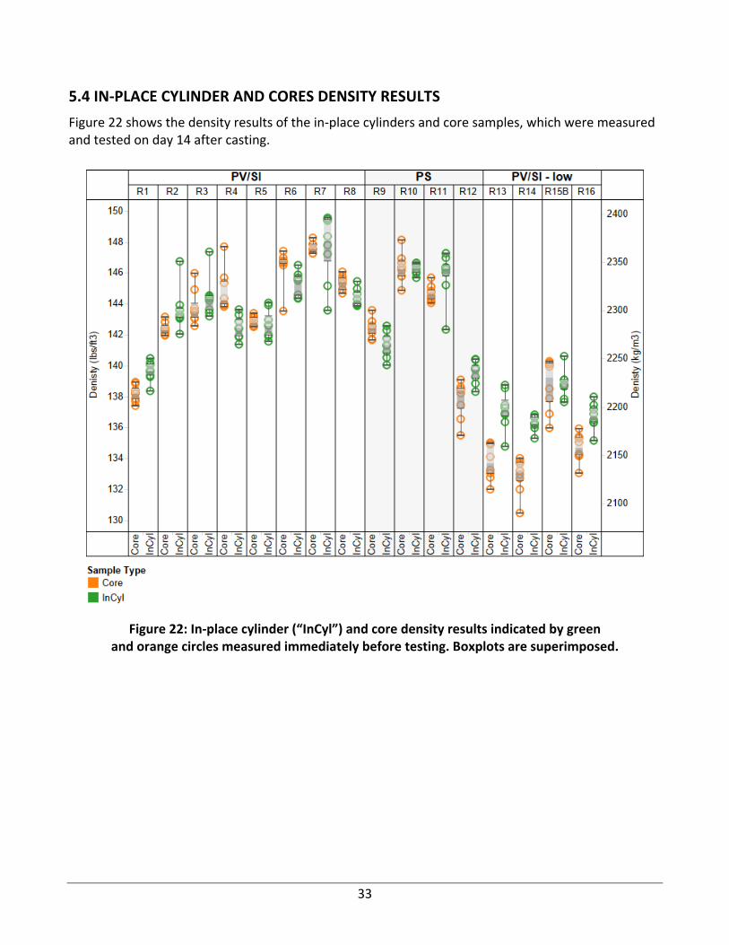
33
5.4 IN‐PLACE CYLINDER AND CORES DENSITY RESULTS
Figure 22 shows the density results of the in‐place cylinders and core samples, which were measured and tested on day 14 after casting.
Figure 22: In‐place cylinder (“InCyl”) and core density results indicated by green and orange circles measured immediately before testing. Boxplots are superimposed.
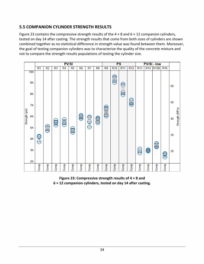
34
5.5 COMPANION CYLINDER STRENGTH RESULTS
Figure 23 contains the compressive strength results of the 4 × 8 and 6 × 12 companion cylinders, tested on day 14 after casting. The strength results that come from both sizes of cylinders are shown combined together as no statistical difference in strength value was found between them. Moreover, the goal of testing companion cylinders was to characterize the quality of the concrete mixture and not to compare the strength results populations of testing the cylinder size.
Figure 23: Compressive strength results of 4 × 8 and 6 × 12 companion cylinders, tested on day 14 after casting.

35
5.6 IN‐PLACE CYLINDER AND CORE COMPRESSIVE STRENGTH RESULTS
Figure 24 contains the compressive strength data of in‐place cylinders and cores, tested in day 16 after casting.
Figure 24: In‐place cylinder (“InCyl”) and core compressive strength results indicated by green and orange circles. Boxplots are superimposed. The fan and the water droplet indicate the 1‐day dry and 1‐day wet slabs. The gray circle with the superimposed orange bar indicates the slabs with
rebar and whether the rebar was in the inner third or outer two‐thirds of the cores.

36
5.7 IN‐PLACE AND CORE DYNAMIC MODULUS RESULTS
Figure 25 contains the longitudinal dynamic elastic modulus results of in‐place cylinders and cores, tested on day 16 after casting.
Figure 25: In‐place cylinder (“InCyl”) and core longitudinal dynamic modulus results indicated by green and orange circles. Boxplots are superimposed. The fan and the water droplet indicate the 1‐day dry and 1‐day wet slabs, respectively. The gray circle with the superimposed orange bar indicates the
slabs with rebar and whether the rebar was in the inner third or outer two‐thirds of the cores.
5.8 EXCLUSION OF SLAB R7 5.8.1 Fresh Concrete Properties
Slab R7 corresponded to the third slab cast with embedded rebar, and the first one in which rebar was located at the cores’ outer two‐thirds. The fresh concrete properties included in Table 4 were employed to accept or reject the delivered concrete at the moment of casting. No additional analyses were carried out with the fresh concrete property data.
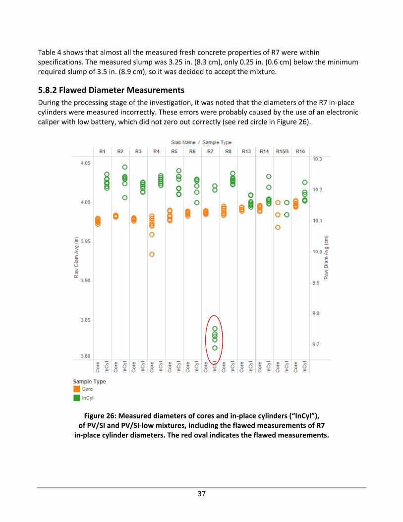
37
Table 4 shows that almost all the measured fresh concrete properties of R7 were within specifications. The measured slump was 3.25 in. (8.3 cm), only 0.25 in. (0.6 cm) below the minimum required slump of 3.5 in. (8.9 cm), so it was decided to accept the mixture.
5.8.2 Flawed Diameter Measurements
During the processing stage of the investigation, it was noted that the diameters of the R7 in‐place cylinders were measured incorrectly. These errors were probably caused by the use of an electronic caliper with low battery, which did not zero out correctly (see red circle in Figure 26).
Figure 26: Measured diameters of cores and in‐place cylinders (“InCyl”), of PV/SI and PV/SI‐low mixtures, including the flawed measurements of R7
in‐place cylinder diameters. The red oval indicates the flawed measurements.

38
5.8.3 Compressive Strength Analysis
R7 was the only slab of the entire set in which in‐place cylinder strength was significantly lower than core strength. This fact is depicted in Figure 27 from a qualitative point of view (statistical analysis confirmed this observation). It should be noted that R7 and R8 cores had steel rebar in the outer two‐thirds, and R5 and R6 cores had rebar in the inner third; the rest of the slab cores did not have rebar.
This unusual result in which the in‐place cylinders of R7 yielded a compressive strength statistically lower than the cores suggested a problem other than the error in the diameters. In addition, looking at slabs R5, R6, and R8, which also contained cores with embedded rebar (as R7 did), it can be seen in Figure 27 that cores always yielded compressive strengths significantly lower than in‐place cylinders did. Thus, it can be presumed that the presence of rebar did not increase the compressive strengths of the cores; instead, the problem should have been in the in‐place cylinders.
Figure 27: Compressive strength of cores and in‐place cylinders (“InCyl”), of PV/SI and PV/SI‐low mixtures, assuming 4 in. (10.2 cm) diameter of the R7 in‐place cylinders to calculate compressive strength. The red arrow indicates the R7 dataset showing that the in‐place cylinder’s compressive
strength population was significantly lower than that of the core population.
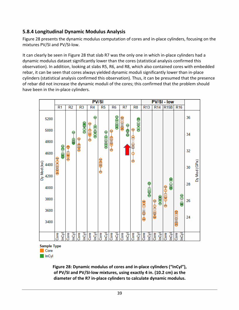
39
5.8.4 Longitudinal Dynamic Modulus Analysis
Figure 28 presents the dynamic modulus computation of cores and in‐place cylinders, focusing on the mixtures PV/SI and PV/SI‐low.
It can clearly be seen in Figure 28 that slab R7 was the only one in which in‐place cylinders had a dynamic modulus dataset significantly lower than the cores (statistical analysis confirmed this observation). In addition, looking at slabs R5, R6, and R8, which also contained cores with embedded rebar, it can be seen that cores always yielded dynamic moduli significantly lower than in‐place cylinders (statistical analysis confirmed this observation). Thus, it can be presumed that the presence of rebar did not increase the dynamic moduli of the cores; this confirmed that the problem should have been in the in‐place cylinders.
Figure 28: Dynamic modulus of cores and in‐place cylinders (“InCyl”), of PV/SI and PV/SI‐low mixtures, using exactly 4 in. (10.2 cm) as the diameter of the R7 in‐place cylinders to calculate dynamic modulus.

40
5.8.5 NDT Analysis
Non‐destructive tests carried out on the slab were compared with the in‐place cylinder compressive strength results to illustrate NDT vs. compressive strength relationships as correlation curves. These analyses are described in detail in Section 5.12.
The goal of including the correlation curves in this section is to give additional support that the in‐place cylinder compressive strength results of slab R7 were flawed and that they should be excluded from the analysis.
Figure 29 depicts the relationship between the rebound hammer test results and in‐place compressive strength results. The dotted line in that figure is an OLS best‐fit line computed for the data without considering R7. The blue dot pointed out by the blue arrow corresponds to R7, which is significantly far from the rest of the population. Assuming that the rebound hammer data were collected accurately, the position in which the R7 blue dot appears suggests that the real R7 average compressive strength should be higher. This explanation suggests that the measured values of compressive strength using the in‐place cylinders were lower than the compressive strength of the concrete that remained in the slab.
A similar graph was obtained when analyzing the pullout test results, with the R7 blue dot being to the right of the graph and significantly away from the rest of the data points. This fact confirms that the NDT measurements taken at the slab’s concrete were accurate and that the in‐place compressive strengths were inaccurate.
Figure 29: Rebound hammer vs. in‐place compressive strength relationship. Blue dots represent the average rebound number vs. average in‐place compressive
strength of each slab. The black horizontal error bars show the variability of all rebound number testing location values. The dotted red line is an OLS best‐fit line computed without
considering R7 results. Blue arrow indicates the averaged data point of R7.
y = 252.99x ‐ 2801.4
0
5
10
15
20
25
30
35
40
45
0
1000
2000
3000
4000
5000
6000
7000
20 25 30 35 40 45
Strength (MPa)
Strength (psi)
Rebound Hammer (Rebound Number)
AveragedData

41
5.8.6 Section Conclusions
The compressive strength values of the in‐place cylinders of slab R7 are not representative of the real in‐place strength of the slab’s concrete. This statement is supported by analyzing compressive strength, dynamic modulus, and rebound hammer test results. The analysis of density comparing in‐place cylinders to cores and in‐place cylinders to companion cylinders, yielded results less clear than the ones presented above. However, it was observed that the in‐place cylinders of R7 have lower densities than they should have, based on a qualitative analysis.
It can also be affirmed that, if the in‐place cylinders’ strengths should have been higher than the measured ones. It is presumed that the concrete exhibited a sticky and dry consistency and thus were more difficult to consolidate within the in‐place cylinders. This explanation justifies the fact that compressive strength and dynamic modulus of the in‐place cylinders were significantly and statistically lower than the compressive strength and dynamic modulus of the cores, respectively, and that their densities were also slightly lower. This fact also explains the findings from the NDT analyses.
As a result of this specific study of slab R7, it was decided to exclude all R7 measurements from the rest of the analysis, discussion, and conclusions.
5.9 STATISTICAL ANOVA ANALYSIS OF IN‐PLACE CYLINDERS VS. CORE STRENGTH
The analysis procedure described in Section 4.3 was applied to each group of data to evaluate the range of correction factors that would make the core strengths not statistically different from the in‐place cylinder strengths. The results of these analyses are described in this section.
5.9.1 Correction Factors
Examining the ranges of correction factors that are applicable to each slab individually, as shown in Figure 30, it is evident that no one correction factor will work for all cores. In particular, the strengths of the wet core treatment required larger and less consistent correction factors to make them statistically similar to the in‐place strengths. Subsequent figures will compare ranges of correction factors applicable to subsets of slabs. Table 5 lists the values of correction factors needed to satisfy a 95% statistical confidence level (giving an F‐score less than or equal to 4.6) for the individual slabs, and combinations thereof, shown in Figure 30. The optimal correction factor (giving an F‐score equal to zero) is also provided for each case. A correction factor score is not provided for the R3 and R4 slab pair because no one factor satisfies both sets of data; as seen in Figure 30, the R3 and R4 slab datasets show no overlap in correction factor value.

42
Figure 30: Correction factors applied to core strengths of each slab to make them not statistically different from the in‐place strengths.
Table 5: Correction Factors Needed to Meet ANOVA Requirements for 95% Confidence Level
Corrections
Min Best Max For pair
R1 1.00 1.05 1.11 1.05
R2 1.02 1.06 1.11
R3 1.12 1.16 1.22 n.a.
R4 1.02 1.06 1.10
R5 1.08 1.11 1.15 1.08
R6 1.01 1.04 1.09
R8 1.05 1.10 1.17 1.10
R9 0.97 1.00 1.04 1.03
R10 0.98 1.09 1.22
R11 1.19 1.22 1.27 1.21
R12 1.12 1.19 1.27
R13 1.00 1.04 1.10 1.05
R14 1.03 1.06 1.11
R15B 1.18 1.23 1.30 1.24
R16 1.21 1.26 1.34

43
The ranges of correction factors applicable to the dry core treatments without rebar are shown in Figure 31. By isolating this subset of slabs, it becomes noticeable that a factor of 1.05 would provide a good prediction of in‐place strength from core strength for the dry core treatments of PV/SI. This is reliable even if extra water were added to lower the strength, as in slabs R13 and R14. With a correction factor of 1.05, the greatest average error of the PV/SI slabs was 0.9%. A factor of 1.03 would be applicable to all six of these slabs, including the higher‐strength PS mix, but with larger overall average errors in prediction. In other words, a correction factor of 1.03 works for all six slabs shown in Fig. 31, but a correction factor of 1.05 provides lower average error in prediction for all slabs except slab R9.
Figure 31: Correction factors applied to dry core strengths of each slab to make them not statistically different from the in‐place strengths.
The ranges of correction factors applicable to the wet core treatments without rebar are shown in Figure 32. A factor of 1.21 would provide a statistically equivalent prediction of in‐place strength from core strength for most but not all of the wet core treatments. The average errors in prediction of in‐place strengths would be significantly higher for those slabs than for the dry core treatment predictions. For slab R4, a factor of 1.21 applied to the core strengths leaves them statistically different from the in‐place strengths.

44
Figure 32: Correction factors applied to wet core strengths of each slab to make them not statistically different from the in‐place strengths.
The ranges of correction factors applicable to the slabs with dry core treatments with rebar are shown in Figure 33. By isolating this subset of slabs, it becomes noticeable that a factor of 1.08 would provide a statistically equivalent prediction of in‐place strength from core strength for the dry core treatments with rebar, except for slab R7, which has been rejected as previously explained. Furthermore, the location of the rebar in the core (located within the inner third of core radius in slabs R5 and R6 and within the outer two‐thirds of the core radius in slab R8) did not significantly affect the correction factor needed to make the core strengths similar to the in‐place strengths. The average errors in prediction of in‐place strengths would be significantly higher for these cores with rebar, but the populations are statistically equivalent to the respective in‐place strengths.

45
Figure 33: Correction factors applied to dry core strengths of slabs containing rebar to make them not statistically different from the in‐place strengths.
5.9.2 Linear Fit
In order to predict the in‐place strength more accurately, a linear fit was also considered to relate the core strength to the in‐place strength. When applied to the dry core data without rebar, the linear fit equation 0.96*(Core Strength) + 337psi yielded strength predictions that were statistically equivalent to the in‐place strength for all six slabs. The greatest average error in the predicted strengths was only 3.7% (Figure 34).

46
Figure 34: Linear fit to dry core strengths of slabs without rebar to make them not statistically different from the in‐place strengths.
5.9.3 Discussion
The results showed high variability between slabs. The most consistent results were achieved by dry conditioning of the cores for the PV/SI mix. For that subset of slabs, the in‐place cylinder strength could be predicted accurately by applying a 1.05 correction factor to the dry core strength. Rebar generally lowers core strengths and increases errors in prediction, but a factor of 1.08 provides strengths that are not statistically different from the in‐place strengths. High‐strength mixes showed more variability, as did the cores with the wet treatment. A linear fit of the data provides a good strength prediction from the cores for both mixes.
5.10 CORE STRENGTH RANDOM SAMPLING ANALYSIS
This section presents the results obtained from applying the random sampling analysis by estimating in‐place strength using cores. Ten different analyses are presented, each corresponding to using a different subset of slabs. These analyses are named alphabetically from A to J, as shown and described in Table 6.
2000 3000 4000 5000 6000 7000 8000 90002000
3000
4000
5000
6000
7000
8000
9000
Core Strength (psi)
In-P
lace
Str
engt
h (p
si)
y = 0.96x + 337

47
Table 6: Core Random Sampling Analyses Description
Analysis Name
Corr. Factor
Slabs Description
A 1.05 R1,R2,R13,R14 PV/SI and PV/SI‐low, no rebar, air dried.
B 1.05 R1,R2,R5,R6,R8,R13,R14 PV/SI and PV/SI‐low, with and without rebar, air dried.
C 1.05 R1,R2 PV/SI only, without rebar, air dried.
D 1.05 R13,R14 PV/SI‐low only, without rebar, air dried.
E 1.08 R5,R6,R8 PV/SI with rebar only, air dried.
F 1.03 R9,R10 PS only, no rebar, air dried.
G 1.05 R1‐R2‐R9‐R10‐R13‐R14 PV/SI, PV/SI‐low and PS, no rebar, air dried.
H 1.05 R1‐R2‐R5‐R6‐R8‐R9‐R10‐
R13‐R14 PV/SI, PV/SI‐low and PS, with and without rebar, air dried.
I 1.03 R1‐R2‐R5‐R6‐R8‐R9‐R10‐
R13‐R14 PV/SI, PV/SI‐low and PS, with and without rebar, air dried.
J Var.*
R1‐R2‐R5‐R6‐R8‐R9‐R10‐R13‐R14 PV/SI, PV/SI‐low and PS, with and without rebar, air dried.
* In analysis J, different correction factors were applied depending on the origin of the strength estimation (i.e., depending of which slab was the core from). The applied correction factors were 1.05 for slabs R1, R2, R13 and R14, 1.08 for slabs R5, R6 and R8, and 1.03 for slabs R9 and R10.
In these analyses it should be noted that the correction factors were computed from the same data that now are being analyzed to quantify the error in strength predictions. Thus, the errors in strength predictions shown here are likely lower than if these factors are applied to a situation with different conditions (e.g. varying mixture design and aggregate size and gradation, different testing age, different sample size, different core conditioning, etc.). It should also be noted that the different analyses consider different number of slabs, which makes the dataset’s sizes to be different, which in turn affect the results’ confidence.
Figure 35 contains the expected error curves of analyses A, B, G, H, I and J. The rest of the expected error curves for analyses C, D, E, and F, as well as the corresponding histograms for all analyses are presented in Appendix E.
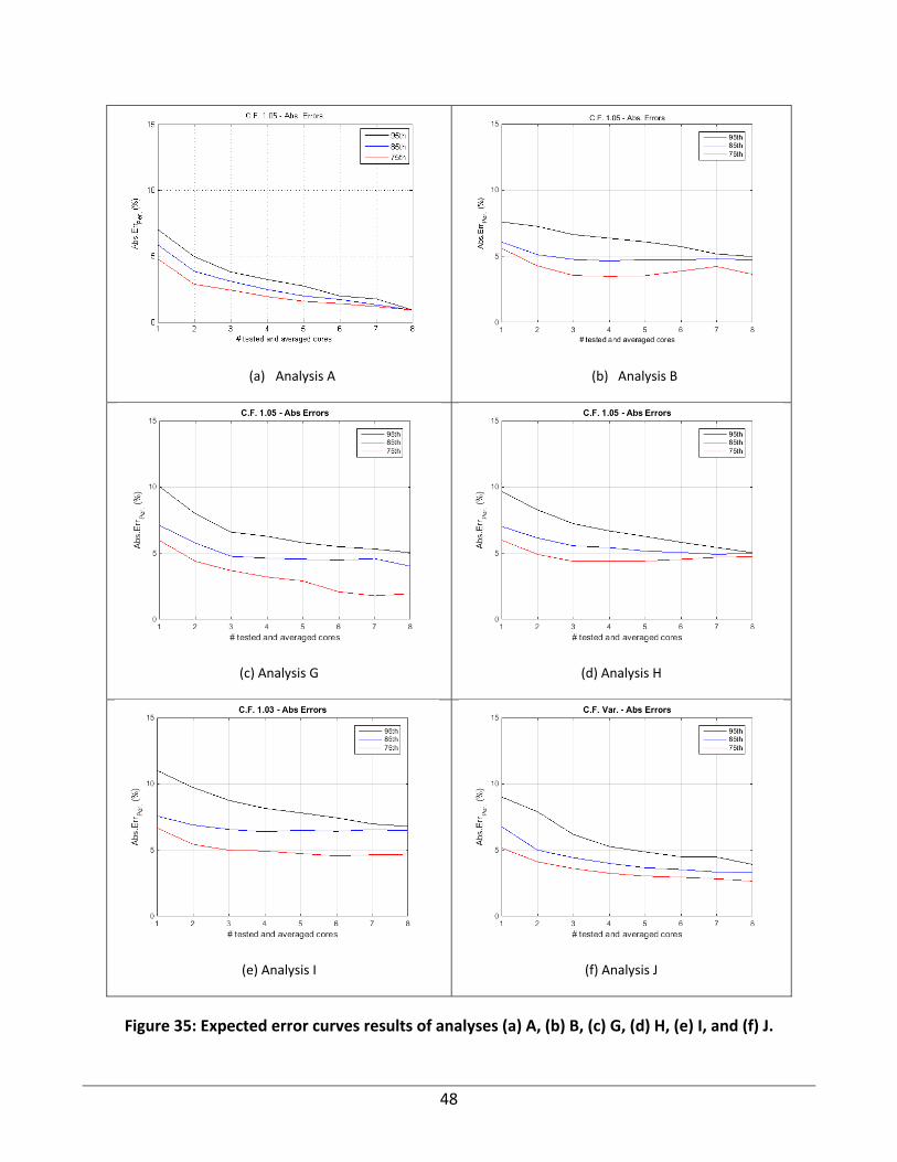
48
(a) Analysis A
(b) Analysis B
(c) Analysis G
(d) Analysis H
(e) Analysis I
(f) Analysis J
Figure 35: Expected error curves results of analyses (a) A, (b) B, (c) G, (d) H, (e) I, and (f) J.

49
The following is a brief description of how to interpret Figure 35.
First it should be noted that theoretically, the expected error curves should never increase with increasing number of cores. This occurs because, for a given level of confidence (a constant percentile in this case), the strength estimation will have a lower error. However, it can be seen in Figure 35, that sometimes the expected error curves tend to increase after six or more # tested and averaged cores are considered; this is an artifact that happens due to the use of limited amount of data, becoming a problem at higher # tested and averaged cores. The Abs.Err.per calculated for 7 and 8 # tested and averaged cores is not as reliable as those obtained for 1 to 6. A well‐established expected error curve would be one that comprises a sufficiently big dataset to provide statistically reliable results. The number of samples considered for each analysis and at each # tested and averaged cores is shown in the corresponding histograms in Appendix E.
To analyze Figure 35, the reader should first select one of the three plotted confidence levels, here quantified as percentiles 75th, 85th and 95th. As an example, consider the 85th percentile, the blue curve in Figure 35. Then choose a value of # tested and averaged cores, for example the value 2. Then the blue curve correlates the value 2 to an expected strength estimation error (Abs.Err.85) in the Y‐axis. That value corresponds to the expected error that has approximately an 85% chance of not being exceeded when averaging two cores. In other words, the error of your strength estimation has an approximately 85% probability of being that obtained error or lower.
A 5% expected error was used under an 85% confidence. It should be noted that previously the correction factors were obtained using a statistical analysis under a 95% confidence level. Those factors were computed comparing populations between in‐place cylinders and cores’ strengths, and using a much more rigorous mathematical/statistical approach. In the analysis presented in this section the approach is less rigorous, as the confidence is only being quantified using the dataset’s percentile. To summarize the difference between these concepts, the computation of every given correction factor was obtained using a 95% confidence level, and in this section, the analysis focuses on the confidence of the strength estimation, which is evaluated using the computed strength error’s dataset’s percentiles.
Figure 35 illustrates that the 85th percentile expected error curves of analyses H and I do not reach 5 % error for any # tested and averaged cores. This fact indicates that considering one single correction factor for all the slabs may not be the most accurate approach. For instance, analysis J contains the same slabs but the correction factors varied depending on the slab; as expected, analysis J had a lower 85th percentile expected curve which intersects the 5% expected error at # tested and averaged cores = 2.
Table 7 has been constructed to provide a better and easier understanding of the results presented in Figure 35, and can be used to draw conclusions by comparing analyses A through J. Table 7 contains the percentage of strength estimations of the random sampling analysis that had a strength error lower than 5% (% Data < 5% error), when considering varying number of tested and averaged cores, for each of the mentioned analyses A to J. In other words, the values presented in Table 7 are the approximate probabilities of obtaining a strength estimation from a core that has an error of 5% or lower, for a given number of averaged cores. For example, using the dataset of analysis A, when two

50
cores are selected randomly from a random slab, and that slab’s in‐place strength is estimated by taking the strength average of those two cores, there is approximately a 96% probability that strength estimation has a 5% error or lower.
The color code in Table 7 indicates the % Data < 5% error lower than 75% exclusively in red, between 75% and 85% exclusively in yellow, and 85% or higher in green.
Table 7: Core Random Sampling Analyses Results
Number of cores used to estimate strength
C.F. Slabs 1 2 3 4 5 6 7 8
%Data < 5% error
A 1.05 R1,R2,R13,R14 78 96 100 100 100 100 100 100
B 1.05 R1,R2,R5,R6,R8,R13,R14 70 84 86 87 88 88 91 100
C 1.05 R1,R2 81 95 100 100 100 100 100 100
D 1.05 R13,R14 75 96 99 100 100 100 100 100
E 1.08 R5,R6,R8 71 79 85 90 93 96 100 100
F 1.03 R9,R10 60 69 75 81 86 91 100 100
G 1.05 R1‐R2‐R9‐R10‐R13‐R14 66 81 86 88 89 90 90 80
H 1.05 R1‐R2‐R5‐R6‐R8‐R9‐R10‐R13‐R14 63 77 80 82 83 84 86 88
I 1.03 R1‐R2‐R5‐R6‐R8‐R9‐R10‐R13‐R14 58 72 75 75 77 77 77 75
J Var. R1‐R2‐R5‐R6‐R8‐R9‐R10‐R13‐R14 72 84 90 93 95 97 100 100
Table 7 clearly shows that the best analyses are A, C and D, where the probability of having a strength estimation error lower than 5% exceeds 85% when using 2 cores. In other words, the green cell with the lowest number of cores occurs at two in these analyses. In these three analyses, only PV/SI and PV/SI‐low were considered, and only the 1.05 correction factor was used. When the rebar slabs are added in analysis B, the first green cell moves one core to the right, but still when taking two cores the result is 84% probability, almost 85% (almost green). Analysis B shows slightly better results than E, which only considers rebar slabs and uses 1.08 correction factor; the reason is because in the latter case the dataset size is much lower than in the former. Similarly, analysis F, which considers PS mixes only, is worse than analysis G—which combines all slabs without rebar. Analysis I, where the 1.03 correction factor is applied to all slabs, shows the poorest results. Analysis H is slightly better than I, and the green cell is achieved only when using 7 cores. Finally, analysis J, which uses the correction factors 1.05 for PV/SI and PV/SI‐low slabs with no rebar, 1.08 for PV/SI slabs with rebar, and 1.03 for PS slabs with no rebar, shows very good results, reaching the green cell at three cores—but with an 84% probability (almost 85%) at two cores.
This study clearly shows that using the correction factors 1.05 for PV/SI cores without rebar, 1.08 for PV/SI cores with rebar, and 1.03 for PS cores without rebar yield the most confident strength estimations. The study also shows that at least two cores are needed, but three are strongly recommended, to reach an approximate 85% confidence of obtaining a strength error of 5% or lower, where the confidence level was quantified using the 85th percentile of the dataset. However, it should be noted that both PS slabs, R9 and R10 showed anomalous behavior which reduces the

51
reliability of the 1.03 correction factor. In the case of R9, the in‐place strength population was very similar to the core strength population, to the point that its optimum correction factor is around 1.00 (see Figure 31). In addition, the R9 in‐place cylinders had statistically lower dynamic moduli than the cores. These facts suggest that some of the R9 in‐place cylinders may have been consolidated poorly. In the case of R10, the core strength results showed large variability (see Figure 24), which made the range of applicable correction factors be much higher than the other slabs, as depicted in Figure 31.
5.11 NDT RESULTS
Before presenting the NDT results, the authors acknowledge that the surface wave results were poor because of experimental problems. The analysis of these results shows that the data had problems; thus, the authors have chosen not to present them nor to show any analysis that may misguide potential upcoming research.
Table 8 presents the number of testing locations per slab and the number of testing replicates per location for each NDT method.
Table 8: Testing Locations per Slab and Testing Replicates per Location for Each NDT
NDT Method Testing Locations per Slab Testing Replicates per Location Total Number of
Measurements per Slab
Rebound 8 10 80
Nitto 8 10 80
Pullout 3* 1 3
*Slab R1 was tested with pullout at five testing locations. Extra tests were carried out because experimental errors occurred that prevented the researchers to collect pullout data on day 16. Thus three pullout measurements were collected on day 17 and two more on day 18 in order to study a potential change due to the hardening concrete in one day. No differences were seen among the collected data, so all five measurements were accepted as valid representation of day 16 data.
Figure 36, Figure 37, and Figure 38 contain the NDT results, divided between mixtures and slabs.
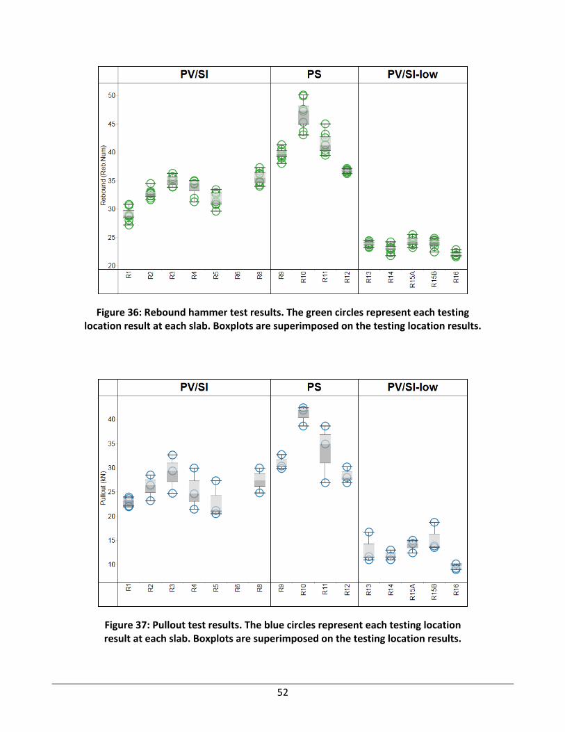
52
Figure 36: Rebound hammer test results. The green circles represent each testing location result at each slab. Boxplots are superimposed on the testing location results.
Figure 37: Pullout test results. The blue circles represent each testing location result at each slab. Boxplots are superimposed on the testing location results.
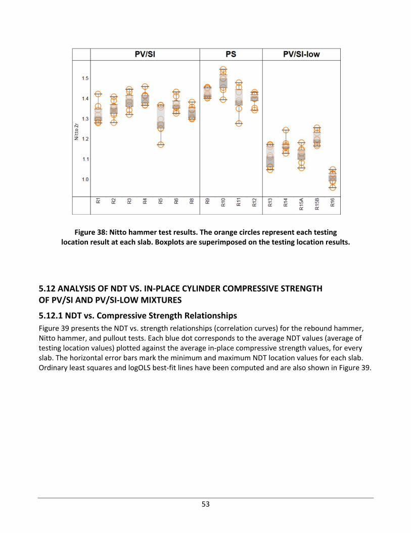
53
Figure 38: Nitto hammer test results. The orange circles represent each testing location result at each slab. Boxplots are superimposed on the testing location results.
5.12 ANALYSIS OF NDT VS. IN‐PLACE CYLINDER COMPRESSIVE STRENGTH OF PV/SI AND PV/SI‐LOW MIXTURES
5.12.1 NDT vs. Compressive Strength Relationships
Figure 39 presents the NDT vs. strength relationships (correlation curves) for the rebound hammer, Nitto hammer, and pullout tests. Each blue dot corresponds to the average NDT values (average of testing location values) plotted against the average in‐place compressive strength values, for every slab. The horizontal error bars mark the minimum and maximum NDT location values for each slab. Ordinary least squares and logOLS best‐fit lines have been computed and are also shown in Figure 39.

54
(a)
(b)
(c)
Figure 39: NDT vs. strength correlation curves for (a) rebound hammer, (b) Nitto hammer, and (c) pullout test, considering PV/SI and PV/SI‐low mixtures only. Blue dots indicate average NDT and strength results of each slab. Horizontal error bars
indicate data range (testing location results) for every slab. Red dotted lines are the best‐fit OLS correlation curves. Gray dotted lines are best‐fit logOLS correlation curves.
It can be seen in Figure 39 that in the cases of the rebound hammer and pullout, the OLS and logOLS best‐fit lines almost overlap. In the case of the Nitto hammer, there are larger differences between the best‐fit lines.
Table 9 contains the useful parameters for the computed OLS and logOLS NDT vs. strength relationships.
Table 9: Computed Parameters for OLS and LogOLS NDT vs. Compressive Strength Relationships
Parameter Rebound,
rebound number Pullout, kN Nitto, Zr
OLS Slope, psi/NDT (MPa/NDT) 253 (1.7) 194 (1.3) 10380 (71.6)
Y‐intercept, psi (MPa) –2801 (–19.3) 628 (4.3) –8464 (–58.4)
LogOLS Factor A 14.78* 393.8* 2236.4*
Exponent B 1.69* 0.817* 3.00*
* Values calculated and valid only for strengths in units of psi.
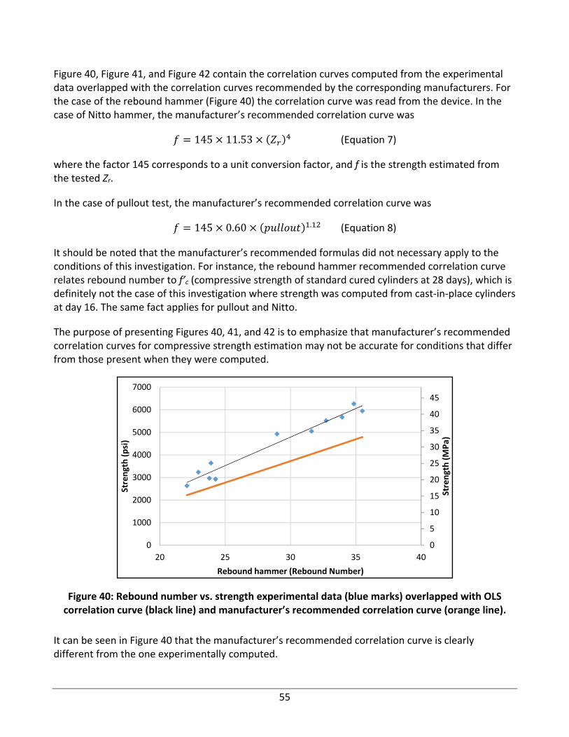
55
Figure 40, Figure 41, and Figure 42 contain the correlation curves computed from the experimental data overlapped with the correlation curves recommended by the corresponding manufacturers. For the case of the rebound hammer (Figure 40) the correlation curve was read from the device. In the case of Nitto hammer, the manufacturer’s recommended correlation curve was
145 11.53 (Equation 7)
where the factor 145 corresponds to a unit conversion factor, and f is the strength estimated from the tested Zr.
In the case of pullout test, the manufacturer’s recommended correlation curve was
145 0.60 . (Equation 8)
It should be noted that the manufacturer’s recommended formulas did not necessary apply to the conditions of this investigation. For instance, the rebound hammer recommended correlation curve relates rebound number to f’c (compressive strength of standard cured cylinders at 28 days), which is definitely not the case of this investigation where strength was computed from cast‐in‐place cylinders at day 16. The same fact applies for pullout and Nitto.
The purpose of presenting Figures 40, 41, and 42 is to emphasize that manufacturer’s recommended correlation curves for compressive strength estimation may not be accurate for conditions that differ from those present when they were computed.
Figure 40: Rebound number vs. strength experimental data (blue marks) overlapped with OLS correlation curve (black line) and manufacturer’s recommended correlation curve (orange line).
It can be seen in Figure 40 that the manufacturer’s recommended correlation curve is clearly different from the one experimentally computed.
0
5
10
15
20
25
30
35
40
45
0
1000
2000
3000
4000
5000
6000
7000
20 25 30 35 40
Strength (MPa)
Strength (psi)
Rebound hammer (Rebound Number)
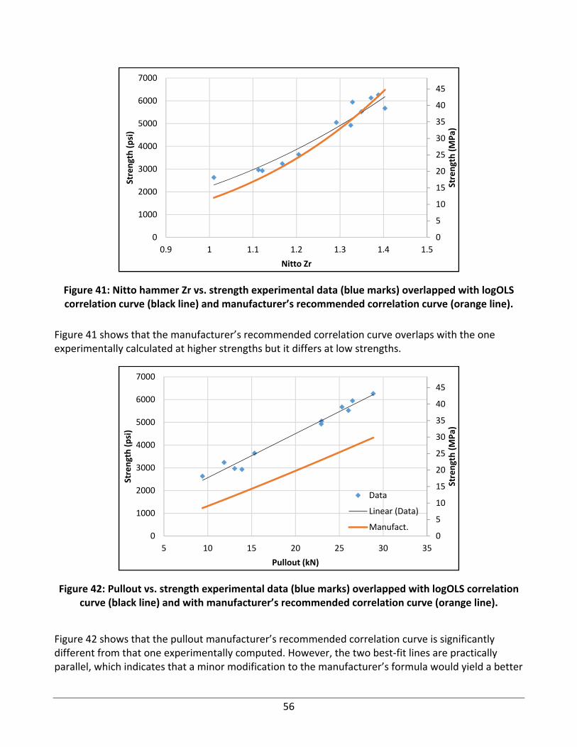
56
Figure 41: Nitto hammer Zr vs. strength experimental data (blue marks) overlapped with logOLS correlation curve (black line) and manufacturer’s recommended correlation curve (orange line).
Figure 41 shows that the manufacturer’s recommended correlation curve overlaps with the one experimentally calculated at higher strengths but it differs at low strengths.
Figure 42: Pullout vs. strength experimental data (blue marks) overlapped with logOLS correlation curve (black line) and with manufacturer’s recommended correlation curve (orange line).
Figure 42 shows that the pullout manufacturer’s recommended correlation curve is significantly different from that one experimentally computed. However, the two best‐fit lines are practically parallel, which indicates that a minor modification to the manufacturer’s formula would yield a better
0
5
10
15
20
25
30
35
40
45
0
1000
2000
3000
4000
5000
6000
7000
0.9 1 1.1 1.2 1.3 1.4 1.5
Strength (MPa)
Strength (psi)
Nitto Zr
0
5
10
15
20
25
30
35
40
45
0
1000
2000
3000
4000
5000
6000
7000
5 10 15 20 25 30 35
Strength (MPa)
Strength (psi)
Pullout (kN)
Data
Linear (Data)
Manufact.
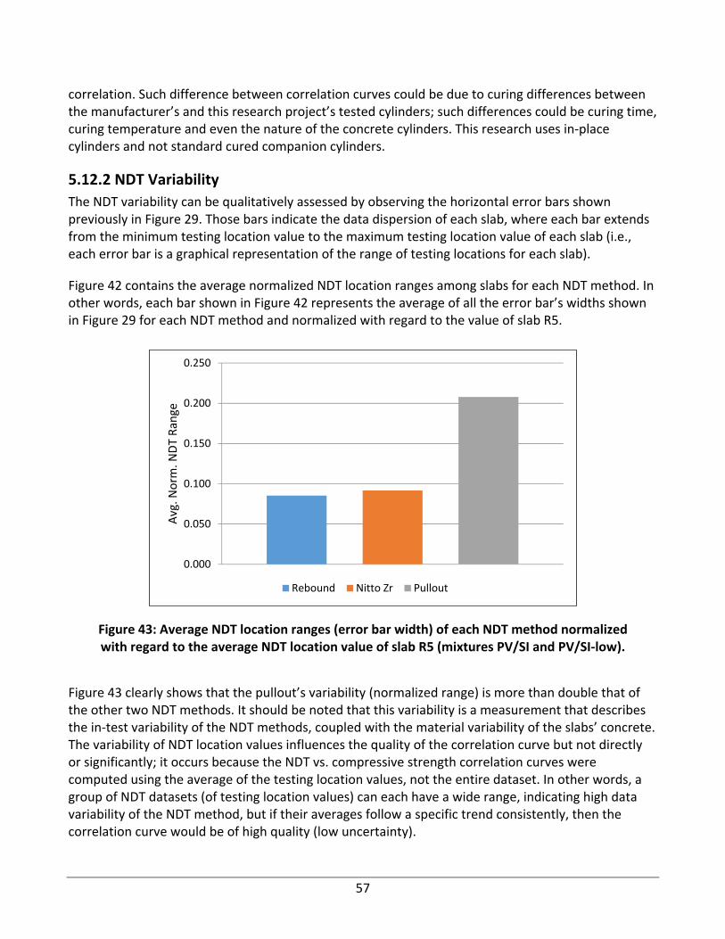
57
correlation. Such difference between correlation curves could be due to curing differences between the manufacturer’s and this research project’s tested cylinders; such differences could be curing time, curing temperature and even the nature of the concrete cylinders. This research uses in‐place cylinders and not standard cured companion cylinders.
5.12.2 NDT Variability
The NDT variability can be qualitatively assessed by observing the horizontal error bars shown previously in Figure 29. Those bars indicate the data dispersion of each slab, where each bar extends from the minimum testing location value to the maximum testing location value of each slab (i.e., each error bar is a graphical representation of the range of testing locations for each slab).
Figure 42 contains the average normalized NDT location ranges among slabs for each NDT method. In other words, each bar shown in Figure 42 represents the average of all the error bar’s widths shown in Figure 29 for each NDT method and normalized with regard to the value of slab R5.
Figure 43: Average NDT location ranges (error bar width) of each NDT method normalized with regard to the average NDT location value of slab R5 (mixtures PV/SI and PV/SI‐low).
Figure 43 clearly shows that the pullout’s variability (normalized range) is more than double that of the other two NDT methods. It should be noted that this variability is a measurement that describes the in‐test variability of the NDT methods, coupled with the material variability of the slabs’ concrete. The variability of NDT location values influences the quality of the correlation curve but not directly or significantly; it occurs because the NDT vs. compressive strength correlation curves were computed using the average of the testing location values, not the entire dataset. In other words, a group of NDT datasets (of testing location values) can each have a wide range, indicating high data variability of the NDT method, but if their averages follow a specific trend consistently, then the correlation curve would be of high quality (low uncertainty).
0.000
0.050
0.100
0.150
0.200
0.250
Avg. N
orm
. NDT Range
Rebound Nitto Zr Pullout

58
5.12.3 Correlation Curve Uncertainty
The uncertainty of the computed correlation curves can be assessed using the RSD parameter, as defined in Section 4.5.3 and by ACI 228 1.R (2003). Figure 44 shows the RSD computed for each NDT method using both the OLS and the logOLS methods.
Figure 44: Residual standard deviation of OLS and logOLS correlation curves relating NDT to in‐place cylinder compressive strength data (mixtures PV/SI and PV/SI‐low).
Figure 44 clearly shows that for both correlation curves, the pullout test has the lowest RSD and the Nitto has the highest. In the case of the OLS computation, the rebound and Nitto hammer tests yielded RSDs 35% and 92% higher, respectively, than the RSD of the pullout. In comparing the RSD results obtained with the logOLS method and the OLS method, it was observed that the RSD of Nitto was reduced, whereas for the rebound and pullout tests, the RSD increased. This fact suggests that using OLS is better for approximating the relationship of the rebound hammer and pullout tests vs. compressive strength, but it is more accurate to use logOLS in the case of Nitto.
5.12.4 NDT Sensitivity
Figure 45 shows the normalized OLS and logOLS NDT vs. strength relationships for the rebound hammer, pullout, and Nitto hammer tests. The pullout test has the lowest slope (or range of slopes for the case of logOLS), followed by the rebound hammer and then the Nitto hammer. This means that the pullout test is the most sensitive, and the Nitto is the least sensitive of the NDT methods.
0
0.5
1
1.5
2
2.5
3
0
50
100
150
200
250
300
350
400
450
Method 1: OLS Method 2: Log OLS
Strength RSD
(MPa)
Strength RSD
(psi)
Rebound Nitto Zr Pullout

59
Figure 45: Analysis of sensitivity showing estimated strength vs. NDT measurements normalized with regard to slab R5. Solid lines and dotted lines correspond to the OLS and logOLS methods, respectively (mixtures PV/SI and PV/SI‐low).
The use of OLS or logOLS did not significantly affect the overall sensitivity of each method of strength determination. Thus, to ease the analysis, sensitivity can be quantified only by observing the slopes of the OLS correlation curves of each NDT method. For the OLS best‐fit lines, a lower slope indicates higher sensitivity than a higher slope.
Table 10 summarizes the normalized slopes of the OLS correlation curves. The pullout test had a normalized slope of 4447 psi (31 MPa) per normalized NDT unit; the normalized slopes of the rebound hammer and Nitto hammer OLS correlation curves were 80% and 200% higher, respectively, than that of pullout test. This analysis clearly shows that pullout test is the most sensitive of the three studied NDT methods.
Table 10: Normalized OLS Slopes and Slopes’ Relative Differences
Rebound Nitto Pullout
Slope, psi/normalized unit (MPa/normalized unit) 7998 (55) 13,407 (92) 4447 (31)
Relative difference (%) 80 201 0
5.12.5 Random Sampling Analysis
The studies presented in the previous sections described the NDT vs. strength relationships and considered their uncertainty. Another study, also discussed previously, assessed the variability of
0
5
10
15
20
25
30
35
40
45
0
1000
2000
3000
4000
5000
6000
7000
0.20 0.40 0.60 0.80 1.00 1.20 1.40
Estimated
Stren
gth (MPa)
Estimated
Stren
gth (psi)
Normalized NDT Measurement
Rebound
Nitto
Pullout

60
each NDT method separately. Those two studies were not combined because they were computed separately. Thus, in general terms, the analysis of the uncertainty of NDT vs. strength relationships could be used to yield an estimated strength from NDT data, but it does not consider the NDT variability. The random sampling analysis combines both approaches by analyzing the trend of the error between real and estimated strengths when additional testing locations are carried out.
Figure 46 contains the results of the random sampling analysis applied when using both types of correlation curves (OLS and logOLS). The Abs.Err95 metric is the value of error between the estimated strength that leaves 95% of the population below it (see Section 4.4 for details on this metric).
Figure 46: Random sampling analysis of (a) rebound hammer, (b) Nitto hammer, and (c) pullout, showing the behavior of Abs.Err95 vs. the considered # NDT locations (mixtures PV/SI and PV/SI‐low).
In the cases of the rebound hammer and pullout tests, the random sampling curves associated with the OLS and logOLS methods are very similar. However, for the Nitto hammer, the logOLS yielded Abs.Err95 values much lower than those of the OLS. This fact is in agreement with the uncertainty analysis shown in Figure 44, where the RSD of the Nitto hammer Zr vs. compressive strength logOLS correlation curve was lower than the RSD of the Nitto hammer Zr vs. compressive strength OLS correlation curve. Thus, this analysis confirms that logOLS is a better approximation method for the Nitto hammer, whereas both OLS and logOLS could be used for the rebound and pullout tests without much difference. Therefore, to simplify the discussion, the OLS results will be further analyzed for rebound hammer and pullout tests, and the logOLS results for the Nitto.
In the case of one testing location, the Abs.Err95 values were 18% for rebound OLS, 24% for Nitto logOLS, and 20% for pullout OLS.

61
For the rebound hammer, when additional testing locations were considered, the Abs.Err95 first decreased and then became constant at # NDT locations equal to three, reaching an Abs.Err95 of 14%. Thus, with the data collected in this investigation, taking more than three rebound hammer testing locations did not reduce the expected strength error significantly.
For the Nitto hammer, the Abs.Err95 decreased with increasing # NDT locations and did not become constant within the eight possible # NDT locations. Only at # NDT locations equal to five did the Abs.Err95 become lower than 14%, meaning that five testing locations with the Nitto hammer would be equivalent to three rebound testing locations to obtain similar expected strength errors.
Finally, in the pullout test, the Abs.Err95 dropped abruptly from 20% to 13% at # NDT locations, and then reached 11% error at # NDT locations equal to three. It also did not appear to have become constant, which indicated that additional testing measurements could reduce the expected error significantly.
To summarize: From this analysis, it can be observed that when carrying out an NDT method at one single testing location, the method that yielded the lowest expected error was the rebound hammer. Carrying out pullout test at two testing locations reached an expected error Abs.Err95 similar to carrying out rebound hammer at three or more testing locations, or Nitto hammer at five or more testing locations. The total lowest expected error was yielded by pullout; at 3 NDT locations the pullout expected error became 11%, which was around 4% lower than the other NDT methods.
5.12.6 Section Conclusions
On the basis of the results presented and discussed in this section, the following can be concluded:
The OLS method yielded more‐accurate correlation curves than logOLS for the rebound hammer and pullout tests; for the Nitto hammer method, the logOLS method yielded more‐accurate results than the OLS.
Based on RSD to assess correlation curve uncertainties, the pullout test (OLS) was the least uncertain, and the Nitto hammer was the most uncertain (both OLS and logOLS curves).
The pullout test had significantly higher NDT variability (within‐test coupled with within‐structure variability) than the other two methods, which, in turn, had similar NDT variability between them.
The pullout test was the most sensitive technique, having an OLS NDT vs. strength slope (normalized) around half of that of the rebound hammer, and a third of that of the Nitto hammer.
When considering only one NDT location, the rebound hammer (OLS) was the method that yielded the lowest expected error (using percentile 95th), with 18%. This error dropped to 14% at three NDT locations and did not change significantly for additional testing locations (i.e., it became constant at three NDT locations). The pullout test (OLS) started with a higher expected error than the rebound hammer when considering one NDT location, but it achieved a 13% expected error with two NDT locations, similar to the rebound hammer at three or more testing locations. Carrying out the pullout test at three locations reduced the expected

62
error to 11%. The Nitto hammer (logOLS) yielded higher expected errors than the rebound hammer and pullout tests at lower # NDT locations, but after five # NDT locations, the expected error became very similar to the other two NDT, reaching expected errors between 11% and 12%.
5.13 ANALYSIS OF NDT VS. IN‐PLACE CYLINDER COMPRESSIVE STRENGTH OF PV/SI, PS, AND PV/SI‐LOW MIXTURES
5.13.1 NDT vs. Compressive Strength Relationships
Figure 47, Figure 48, and Figure 49 present the NDT vs. strength relationships (correlation curves) for the rebound hammer, Nitto hammer and pullout tests, respectively. Each blue dot corresponds to the average NDT values (average of testing location values) plotted against the average in‐place compressive strength values, for every slab. The horizontal error bars mark the minimum and maximum NDT location values for each slab. The ordinary least squares and logOLS best‐fit lines have been computed and are also shown in the figures.
Figure 47: Rebound hammer NDT vs. strength correlation curves for PV/SI, PS, and PV/SI‐low mixtures. Blue dots indicate average NDT and strength results of each slab. Horizontal error bars indicate data range (testing location results) for every slab. Red dotted lines are the
best‐fit OLS correlation curves. Gray dotted lines are best‐fit logOLS correlation curves.
0
10
20
30
40
50
60
70
80
0
2000
4000
6000
8000
10000
12000
20 25 30 35 40 45 50 55
Strength (MPa)
Strength (psi)
Rebound Hammer (Rebound Number)
Averaged Data
OLS
LogOLS

63
Figure 48: Nitto hammer NDT vs. strength correlation curves for PV/SI, PS, and PV/SI‐low mixtures. Blue dots indicate average NDT and strength results of each slab. Horizontal
error bars indicate data range (testing location results) for every slab. Red dotted lines are the best‐fit OLS correlation curves. Gray dotted lines are best‐fit logOLS correlation curves.
Figure 49: Pullout test NDT vs. strength correlation curves for PV/SI, PS, and PV/SI‐low mixtures. Blue dots indicate average NDT and strength results of each slab. Horizontal
error bars indicate data range (testing location results) for every slab. Red dotted lines are the best‐fit OLS correlation curves. Gray dotted lines are best‐fit logOLS correlation curves.
0
10
20
30
40
50
60
70
80
0
2000
4000
6000
8000
10000
12000
0.90 1.00 1.10 1.20 1.30 1.40 1.50 1.60
Strength (MPa)
Strength (psi)
Nitto Zr
Averaged Data
OLS
LogOLS
0
10
20
30
40
50
60
70
80
0
2000
4000
6000
8000
10000
12000
5 10 15 20 25 30 35 40 45
Strength (MPa)
Strength (psi)
Pullout (kN)
Averaged Data
OLS
LogOLS

64
It can be seen in Figures 46 and 48 that for the rebound hammer and pullout tests, the OLS and logOLS best‐fit lines almost overlap, except for edges of the curves. For the Nitto hammer, shown in Figure 48, there are larger differences between the best‐fit lines. The same observations were presented in Section 5.13.1 for the analysis of PV/SI and PV/SI‐low.
Table 11 contains the parameters of the computed OLS and logOLS NDT vs. strength relationships.
Table 11: Computed Parameters of OLS and LogOLS NDT vs. Compressive Strength Relationships for PV/SI, PS, and PV/SI‐Low Mixtures
Parameter Rebound,
rebound number Pullout, kN Nitto, Zr
OLS Slope, psi/NDT (MPa/NDT) 263 (1.81) 13229 (91.21) 220 (1.51)
Y‐intercept, psi (MPa) –3041 (–20.97) –11769 (–81.14) 225 (1.55)
LogOLS Factor A 17.83* 2121.82* 315.16*
Exponent B 1.64* 3.40* 0.90*
* Values calculated and valid only for strengths in units of psi.
5.13.2 NDT Variability
The NDT variability can be qualitatively assessed by observing the horizontal error bars in Figure 47 through Figure 49. Those bars indicate the data dispersion of each slab, where each bar extends from the minimum testing location value to the maximum testing location value of each slab (i.e., each error bar is a graphical representation of the range of testing locations for each slab).
Figure 50 contains the normalized average NDT location ranges among slabs for each NDT method. In other words, each bar shown in Figure 50 represents the average of all the error bar widths shown in Figures 47, 48, and 49 for each NDT method, and normalized with regard to the value of R5.
Figure 50: Average NDT location ranges (error bar width) of each NDT method normalized with regard to the average NDT location value of slab R5 (mixtures PV/SI, PS, and PV/SI‐low ).
0.000
0.050
0.100
0.150
0.200
0.250
Avg. N
orm
. NDT Range
Rebound Nitto Zr CAPOPullout
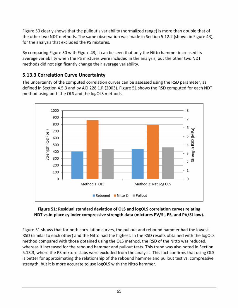
65
Figure 50 clearly shows that the pullout’s variability (normalized range) is more than double that of the other two NDT methods. The same observation was made in Section 5.12.2 (shown in Figure 43), for the analysis that excluded the PS mixtures.
By comparing Figure 50 with Figure 43, it can be seen that only the Nitto hammer increased its average variability when the PS mixtures were included in the analysis, but the other two NDT methods did not significantly change their average variability.
5.13.3 Correlation Curve Uncertainty
The uncertainty of the computed correlation curves can be assessed using the RSD parameter, as defined in Section 4.5.3 and by ACI 228 1.R (2003). Figure 51 shows the RSD computed for each NDT method using both the OLS and the logOLS methods.
Figure 51: Residual standard deviation of OLS and logOLS correlation curves relating NDT vs.in‐place cylinder compressive strength data (mixtures PV/SI, PS, and PV/SI‐low).
Figure 51 shows that for both correlation curves, the pullout and rebound hammer had the lowest RSD (similar to each other) and the Nitto had the highest. In the RSD results obtained with the logOLS method compared with those obtained using the OLS method, the RSD of the Nitto was reduced, whereas it increased for the rebound hammer and pullout tests. This trend was also noted in Section 5.13.3, where the PS mixture slabs were excluded from the analysis. This fact confirms that using OLS is better for approximating the relationship of the rebound hammer and pullout test vs. compressive strength, but it is more accurate to use logOLS with the Nitto hammer.
0
1
2
3
4
5
6
7
8
0
100
200
300
400
500
600
700
800
900
1000
Method 1: OLS Method 2: Nat Log OLS
Strength RSD
(MPa)
Strength RSD
(psi)
Rebound Nitto Zr Pullout

66
5.13.4 NDT Sensitivity
Figure 52 shows the normalized OLS and logOLS NDT vs. strength relationships for the rebound hammer, Nitto hammer, and pullout tests. It can clearly be seen that the pullout test had the lowest slope (or range of slopes in the case of logOLS), followed by the rebound hammer and then the Nitto hammer. This means that, when considering PS mixture slabs, the pullout test is again the most sensitive and the Nitto is the least sensitive of the NDT methods.
Figure 52: Analysis of sensitivity showing estimated strength vs. NDT location data normalized with regard to slab R5. Solid lines and dotted lines correspond to
OLS and logOLS methods, respectively (mixtures PV/SI, PS, and PV/SI‐low).
As it was discussed in Section 5.13.4, the use of OLS or logOLS does not significantly affect the overall sensitivity of each method of strength determination. Thus, to simplify the analysis, sensitivity can be quantified by observing only the slopes of the OLS correlation curves of each NDT method. With the OLS best‐fit lines, a lower slope indicates higher sensitivity than a higher slope.
Table 12 summarizes the normalized slopes of the OLS correlation curves. The pullout test had a normalized slope of 4447 psi (31 MPa) per normalized NDT unit; the normalized slopes of the rebound hammer and Nitto hammer OLS correlation curves were 80% and 200% higher, respectively, than those of the pullout test. This analysis clearly shows that pullout test is the most sensitive of the three studied NDT methods.
0
10
20
30
40
50
60
70
80
0
2000
4000
6000
8000
10000
12000
0.00 0.50 1.00 1.50 2.00
Estimated
Stren
gth (MPa)
Estimated
Stren
gth (psi)
Normalized NDT Measurement
Rebound
Nitto
Pullout

67
Table 12: Normalized OLS Slopes and Slopes’ Relative Differences for Mixtures PV/SI, PS, and PV/SI‐Low Analyzed Together
Rebound,
rebound number Nitto, Zr Pullout, kN
Slope, psi/normalized unit (MPa/normalized unit) 8298 (57) 17087 (118) 5043 (35)
Relative difference (%) 65 239 0
5.13.5 Random Sampling Analysis
This analysis is analogous to the one explained in Section 5.13.5. Figure 53 contains the results of the random sampling analysis when using both types of correlation curves (OLS and logOLS). The Abs.Err95 metric is the value of error between the estimated strength that leaves 95% of the population below it (see Section 4.4 for details on this metric).
Figure 53: Random sampling analysis of (a) rebound hammer, (b) Nitto hammer, and (c) pullout, showing the behavior of the Abs.Err95
metric vs. # NDT locations (mixtures PV/SI, PS, and PV/SI‐low).
Figure 53 shows the same trends as the ones observed in Figure 46 for the PV/SI and PV/SI‐low analysis that excluded the PS mixture. However, when the PS mixture slabs were included in the analysis, the Abs.Err95 parameter tended to shift around 5% to higher values; this fact is graphically depicted by observing that in Figure 53, the Abs.Err95 curves tend to be displaced around 5%, to higher values than the corresponding Abs.Err95 curves in Figure 46. This means that using the PS

68
mixture with the other mixtures increased the expected strength errors given by the correlation curves.
It can be seen in Figure 53 that at three testing locations, both the rebound hammer and pullout tests had the same Abs.Err95. However, the Nitto hammer yielded poor Abs.Err95 results, even for seven and eight testing locations. The OLS Abs.Err95 curve is not shown because it had values higher than 30%, indicating very high inaccuracy in estimating strength.
5.13.6 Section Conclusions The same conclusions can be drawn as those in Section 5.13.6, with the following differences/additions:
Including the PS mixture slabs tended to increase the Abs.Err95 by approximately 5% more than when it was not included. This was not an unexpected result given that the PS mixture was a nominally different mixture design with different aggregate sizes and proportions. In addition, it was seen that PS mixture slabs had more variable fresh and hardened concrete properties than the other two mixtures.
The use of the Nitto hammer for strength estimations when the PS mixture is included was inaccurate, yielding expected error results higher than 23%.
The rebound hammer had a slightly better performance than the pullout test, reaching expected strength errors of less than 15% for two or more testing locations, whereas the pullout test reached the 15% expected error at two testing locations and 12% at three testing locations.

69
CHAPTER 6: CONCLUSIONS
The objectives of this research were to evaluate core strength correction factors considering a range of pertinent factors that are encountered in the field, and to investigate more practical core field curing practices that provide acceptable estimates of in‐place concrete strength. The in‐place strength was established by testing in‐place cylinders at day 16 after casting. It should be noted that this approach is different to the factors given elsewhere, for example in ACI 214.4R (2010), which are provided to estimate f’c obtained using conditioned cores after extraction.
The following conclusions can be drawn from the results and discussion presented in the report.
Regarding the number of core samples to use to estimate in‐place strength, the results confirm that increasing number of core samples extracted from a given mixture improves the in‐place strength estimate of that mixture where the average of core sample strengths are used in the estimation.
Assuming that 1‐day‐dry core treatment is used along with the 1.05 correction factor for core samples from PV‐SI and PV‐SI‐low mixtures that do not contain embedded rebar (based on analysis A with data from slab samples R1, R2, R13 and R14), the average of two cores is needed to provide at least a 95% likelihood of having an absolute error of 5% or lower with respect to the actual in‐place strength.
Assuming that 1‐day‐dry core treatment is used along with the 1.05 correction factor for core samples from PV‐SI and PV‐SI‐low mixtures that both do and do not contain embedded rebar (based on analysis B with data from slab samples R1, R2, R5, R6, R8, R13 and R14), the average of three cores is needed to provide at least an 85% likelihood of having an absolute error of 5% or lower with respect to the actual in‐place strength.
Now considering all three mixture types together for the case of slabs with and without embedded rebar (based on analysis J with data from slab samples R1, R2, R5, R6, R8, R9, R10, R13, and R14), assuming that 1‐day‐dry core treatment is used along with the 1.05 correction factor for core samples from PV‐SI and PV‐SI‐low mixtures, a 1.08 correction factor for core samples from PV‐SI mixture with embedded rebar and 1.03 correction factor for core samples from PS mixtures without rebar, the average of three cores is needed to provide at least a 90% likelihood of having an absolute error of 5% or lower with respect to the actual in‐place strength.
The position of the rebar within the cross‐section did not have a significant effect on the results.
NDT conclusions:
o All NDT methods showed positive correlation with in‐place strength. Linear correlation curves (OLS) were found to be more appropriate than the power correlation curve (LogOLS) for the rebound hammer and pullout test data, and the opposite was found for Nitto hammer data.

70
o For each NDT method, correlations curves established using only PV/SI and PV/SI‐low mixtures were more certain than when including the PS mixture in the analysis.
o Each NDT method exhibited benefits and drawbacks. The Nitto hammer and rebound hammer were easier and faster to carry out as compared with the pullout test in in terms of collecting data from a single testing location. On the other hand, pullout was the most sensitive to in‐place strength and Nitto the least.
o The confidence in the strength estimation from NDT increased with data from increasing number of testing locations. Random sampling analysis showed that, for the same number of testing locations, pullout and rebound tests had similar expected error in the estimated strengths (Abs.Err.95), whereas Nitto hammer had higher expected errors. For one single testing location, rebound yielded the lowest expected error and Nitto the highest; for two or more testing locations pullout yielded the lowest expected error and Nitto hammer the highest.
o For rebound hammer, in the analysis excluding the PS mixture, carrying out more than four testing locations did not reduce the expected error any further; i.e., carrying out a fifth test location with rebound hammer did not reduce the expected error of the estimated strength. At four or more testing locations, the rebound hammer expected error was equivalent to the expected error of pullout at two testing locations. Carrying out pullout at three testing locations yielded the least expected error.
71
CHAPTER 7: RECOMMENDATIONS
On the basis of the experimental results and analysis of this investigation, which consider cores and in‐place cylinders tested 16 days after casting, the following recommendations are offered:
It is beneficial to employ the fan dry core treatment described here as an option to the AASHTO T 24 standard in order to obtain core test samples more rapidly. Furthermore, it is beneficial to the State Agency to apply correction factors described in this report to obtain reliable in‐place compressive strength estimates obtained from those core samples.
It is possible and beneficial to use the rebound hammer, and/or pullout NDT methods to reduce the number of cores to be drawn from a concrete structure. Correlation curves can be constructed according to ACI 228.1R (2003) to correlate NDT measurements to in‐place strength yielding estimates with expected errors of less than 15% at a 95% confidence level. Using a well‐established correlation curve, either the rebound hammer or pullout can be carried out in one testing location to obtain fairly accurate strength estimation. Three testing locations per batch are enough to achieve good accuracy.
Further research is needed to establish the behavior of concrete with higher strength, greater age after casting, and larger aggregate sizes and core samples exposed to different treatments.

72
REFERENCES
ACI 214.4R, “Guide for obtaining cores and interpreting compressive strength results.” American Concrete Institute, Farmington Hills, MI, 2010.
ACI 228.1R, “In‐place methods to estimate concrete strength.” American Concrete Institute, Farmington Hills, MI, 2003.
ACI 318, “Building code requirements for structural concrete.” American Concrete Institute, Farmington Hills, MI, 2010.
Arıöz, M., Tuncan, M., Ramyar, K. and Tuncan, A., “A comparative study on the interpretation of concrete core strength results.” Magazine of Concrete Research, Vol. 58, No. 2, pp. 117‐122, 2006
ASTM C 39/C 39M‐12a. “Standard test method for compressive strength of cylindrical concrete specimens.” ASTM International, West Conshohocken, PA, 2012.
ASTM C 143/C 143M‐15a. “Standard test method for slump of hydraulic‐cement concrete.” ASTM International, West Conshohocken, PA, 2015.
ASTM C 192/C 192M‐13a. “Standard practice for making and curing concrete test specimens in the laboratory.” ASTM International, West Conshohocken, PA, 2013.
ASTM C 215‐02. “Standard test method for fundamental transverse, longitudinal, and torsional resonant frequencies of concrete specimens.” ASTM International, West Conshohocken, PA, 2002.
ASTM C 231/C 231M‐16. “Standard test method for air content of freshly mixed concrete by the pressure method.” ASTM International, West Conshohocken, PA, 2016.
ASTM C 805. “Standard test method for rebound number of hardened concrete.” ASTM International, West Conshohocken, PA, 2002.
ASTM C 873. “Standard test method for compressive strength of concrete cylinders cast in place in cylindrical molds.” ASTM International, West Conshohocken, PA, 2002.
ASTM C 900. “Standard test method for pullout strength of hardened concrete.” ASTM International, West Conshohocken, PA, 2013.
Gaynor, R.D. “Effect of horizontal reinforcing steel on the strength of molded cylinders.” Journal of the American Concrete Institute, Vol. 62, No. 7, pp. 837‐840, 1965.
Mindess, S., Young, J.F., and Darwin, D. Concrete. Pearson Education, Inc., 2nd edition, 2003.
Nikbin, I.M., Eslami, M. and Rezvani, S.M.D. “An experimental comparative survey on the interpretation of concrete core strength results.” European Journal of Scientific Research, Vol. 37, No. 3, pp. 445‐456, 2009.

73
APPENDIX A: TABLES OF RESULTS
Table A.1: Full Fresh Concrete Experimental Results, Part 1
Slab Name Casting Day
Slump (in)
Uncorrected Air (%)
Corrected Air (%)
Measured Weight (lb)
Unit weight (lb/ft3)
R1 Jul‐29‐2014 4.5 8.4 8 41 134
R2 Aug‐05‐2014 4.25 5.3 4.9 43.5 144
R3 Aug‐12‐2014 4.25 6.2 5.8 43 142
R4 Aug‐19‐2014 4 6.2 5.8 44 146
R5 Sep‐02‐2014 4.75 7 6.6 43 142
R6 Sep‐16‐2014 4.5 6.2 5.8 43.5 144
R7 Sep‐23‐2014 3.25 8 7.6 43 142
R8 Sep‐30‐2014 3.5 6 5.6 43.5 144
R9 Oct‐07‐2014 4.75 7 6.6 42.5 140
R10 Oct‐21‐2014 4 5.5 5.1 44 146
R11 Oct‐28‐2014 3.75 6.5 6.1 ‐ ‐
R12 Nov‐5‐2014 7 8.3 7.9 ‐ ‐
R13 Nov‐4‐2014 8–9 9.5 9.1 42 138
R14 Nov‐10‐2014 8.75 10 9.6 41 134
R15 Nov‐19‐2014 8 8.5 8.1 ‐ ‐
R16 Nov‐24‐2014 8 9.5 9.1 41.5 136
R15B Jan‐21‐2015 7.75 8.4 8 43 142
Table A.2: Full Fresh Concrete Experimental Results, Part 2
Slab Name Observations
R1 First slump test gave 5.5 in. Second slump test performed after 10 minutes gave 4.5 in.
R2 Air is 0.1 % out of spec (spec 5 to 8 %).
R3 First slump test gave 3.75 in. Super was added and gave 6.5 in. 5 minutes after slump was 5. Finally 10 minutes after the last test the slump was 4.25 in.
R4
R5
R6
R7
R8
R9
R10
Upon arrival, half gallon of super was added and tests yielded 0.25 in slump and 2.5 % uncorrected air. Then 1 additional gal. of super and 20 oz of AEA were added, and tests yielded the final results. The resulting concrete had very high slump loss. Thus, the vibration was harsh and finishing was tough too; the resulting surface had to be wetted to enable steel troweling and still was not smooth.
R11
R12 Upon arrival, at 1:20pm tests gave: slump 7 in, UW + bucket = 41.5 lb and uncorrected air 11%. Concrete was submitted to 40 rev and the uncorrected air was reduced to 10.5 %. Then the concrete was let to sit for 10 minutes and the new (final) uncorrected air was obtained.
R13 Slump measurement was not registered but it was between 8 and 9 in
R14 Slab was kept with the burlap bags on for three days more than it was supposed to (a weekend).
R15 Curing done for 2.5 days instead of 3 days—WRONG CORING. Cores were drawn one day before they were supposed to and in‐place were also drawn one day before. Tests were done in the correct day. This slab was not used to in the discussion nor to draw final conclusions.
R16
R15B Moist curing done for 4 days instead of 3 days.

74
TABLE A.3 (MULTI‐PART)
In the tables on the following pages, cells colored with blue are direct measurements, and cells not colored are
calculated results. Cells colored in yellow indicate the existence of comments, sometimes unimportant. “Range
dif.” is the range of the corresponding dataset (cores or in‐place cylinders’ strength datasets) divided by its
mean, expressed in %, “L/D” is the aspect ratio and, in the column titled Type of Break, “exp” indicates that the
specimen exploded during compressive strength testing

75
Table A.3: Companion, Core, and In‐Place Cylinders’ Compressive Strength Test Results, Part 1
CROSS-SECTIONAL
AREALOAD
mm mm mm mm in2 lbs.
- day - Top Bot Top Bot 1 2 3 Ave 1 2 Ave L/D Ave -
1 Aug-12-14 14 Comp_1 2 1 1 1 8.0313 8 8 8.01 4.047 4.007 4.027 1.989 12.74 54975
2 Aug-12-14 14 Comp_2 1 1 1 0 8 8.0313 8.0313 8.02 4.04 4.003 4.022 1.994 12.70 53875
3 Aug-12-14 14 Comp_3 1 2 1 0 7.9688 8.0313 8.0313 8.01 4.029 4.029 4.029 1.988 12.75 53755
4 Aug-12-14 14 Comp_4 0 2 0 0 12.063 12.063 12.063 12.06 6.021 6.003 6.012 2.006 28.39 119060
5 Aug-12-14 14 Comp_5 2 2 0 0 12.031 12.063 12.023 12.04 5.948 5.993 5.971 2.016 28.00 119020
6 Aug-14-14 16 Core_1 2 0 1 2 8.125 8.0938 8.0938 8.10 3.976 3.976 3.976 2.038 12.42 55650
7 Aug-14-14 16 Core_2 0 1 0 0 8.0938 8.125 8.0938 8.10 3.98 3.98 3.980 2.036 12.44 59580
8 Aug-14-14 16 Core_3 1 0 1 1 8.0938 8.0938 8.125 8.10 3.975 3.977 3.976 2.038 12.42 58120
9 Aug-14-14 16 Core_4 0 0 0 0 8.0938 8 8 8.03 3.972 3.977 3.975 2.021 12.41 62685
10 Aug-14-14 16 Core_5 0 0 0 2 8.0313 8.125 8.0938 8.08 3.981 3.977 3.979 2.031 12.43 56705
11 Aug-14-14 16 Core_6 0 0 0 0 8.0938 8.125 8.0938 8.10 3.977 3.977 3.977 2.038 12.42 60375
12 Aug-14-14 16 Core_7 0 0 0 0 8.1563 8.0625 8.125 8.11 3.972 3.973 3.973 2.043 12.39 54020
13 Aug-14-14 16 Core_8 0 1 0 0 8 8.0625 8.0938 8.05 3.976 3.975 3.976 2.025 12.41 59050
14 Aug-14-14 16 InCyl_1 0 0 3 0 8.0625 8.0625 8.0938 8.07 4.072 3.987 4.030 2.003 12.75 66585
15 Aug-14-14 16 InCyl_2 0 0 2 1 8 8.0625 8.0313 8.03 4.023 4.025 4.024 1.996 12.72 61160
16 Aug-14-14 16 InCyl_3 0 0 1 1 8.0625 8.0625 8.0938 8.07 4.028 4.013 4.021 2.008 12.70 65715
17 Aug-14-14 16 InCyl_4 0 0 0 0 8 8.0625 8.0625 8.04 4.023 4.028 4.026 1.998 12.73 57560
18 Aug-14-14 16 InCyl_5 0 0 4 1 8 8 8 8.00 4.014 4.058 4.036 1.982 12.79 61965
19 Aug-14-14 16 InCyl_6 0 0 1 1 8 8 8.0313 8.01 4.002 4.049 4.026 1.990 12.73 61205
20 Aug-14-14 16 InCyl_7 0 0 2 0 8 8.0313 8.0313 8.02 4.027 4.01 4.019 1.996 12.68 64470
21 Aug-14-14 16 InCyl_8 0 0 0 0 8 8 8.0313 8.01 4.014 4.047 4.031 1.987 12.76 62890
22 Aug-21-14 14 Comp_1 1 1 3 0 8.25 8.0625 8.0313 8.11 4.055 4.023 4.039 2.009 12.81 64155
23 Aug-21-14 14 Comp_2 2 2 0 0 8 8.0938 8.0313 8.04 4.024 4.03 4.027 1.997 12.74 65630
24 Aug-21-14 14 Comp_3 4 3 0 0 8.0625 8.0313 8.25 8.11 4.087 3.948 4.018 2.020 12.68 NaN
25 Aug-21-14 14 Comp_4 1 1 2 1 12.063 12.063 12 12.04 5.972 6.008 5.990 2.010 28.18 134070
26 Aug-21-14 14 Comp_5 5 1 3 0 12.125 12.063 12.063 12.08 6.007 5.995 6.001 2.014 28.28 135140
27 Aug-21-14 16 Core_1 3 0 0 0 8 7.9688 7.9688 7.98 3.982 3.981 3.982 2.004 12.45 62840
28 Aug-21-14 16 Core_2 5 1 0 0 8.0625 8.0938 7.9375 8.03 3.981 3.982 3.982 2.017 12.45 65075
29 Aug-21-14 16 Core_3 2 0 0 0 8.0313 8 8 8.01 3.983 3.982 3.983 2.011 12.46 65095
30 Aug-21-14 16 Core_4 3 0 0 0 7.9688 7.9688 7.9375 7.96 3.983 3.982 3.983 1.998 12.46 64655
31 Aug-21-14 16 Core_5 1 1 0 0 8 8 8.0313 8.01 3.983 3.984 3.984 2.011 12.46 62905
32 Aug-21-14 16 Core_6 3 0 0 0 7.9688 7.9375 7.9375 7.95 3.982 3.982 3.982 1.996 12.45 69420
33 Aug-21-14 16 Core_7 2 1 0 0 8 8.0313 8.0625 8.03 3.983 3.982 3.983 2.017 12.46 62405
34 Aug-21-14 16 Core_8 1 0 0 0 7.9688 8 7.9688 7.98 3.984 3.984 3.984 2.003 12.47 68135
35 Aug-21-14 16 InCyl_1 0 0 1 0 8.0313 8.0938 8.0625 8.06 4.025 4.023 4.024 2.004 12.72 69530
36 Aug-21-14 16 InCyl_2 3 1 2 0 8.0938 8.1563 8.0938 8.11 3.994 4.067 4.031 2.013 12.76 73975
37 Aug-21-14 16 InCyl_3 3 0 1 1 8.125 8.0625 8.125 8.10 4.043 4.017 4.030 2.011 12.76 67840
38 Aug-21-14 16 InCyl_4 3 0 0 0 8.125 8.1875 8.0938 8.14 4.042 4.025 4.034 2.017 12.78 69930
39 Aug-21-14 16 InCyl_5 2 0 0 1 8.0313 8 8.0313 8.02 4.043 4.021 4.032 1.989 12.77 74655
40 Aug-21-14 16 InCyl_6 0 0 2 1 8.125 8.0938 8.1563 8.13 4.044 4.046 4.045 2.009 12.85 69590
41 Aug-21-14 16 InCyl_7 1 0 0 0 8.0625 8.0938 8.0625 8.07 4.045 4.022 4.034 2.001 12.78 71915
42 Aug-21-14 16 InCyl_8 1 0 0 1 7.9375 7.9688 7.9688 7.96 4.012 4.001 4.007 1.986 12.61 65705
STRENGTHDATE
Age of Conc at testing
GROUP/SAMPLE ID
NUMBER
RoughnessPerpendicul
arityHEIGHT DIAMETER
-
inch inch psi
4482
4789
4681
5053
4560
4860
4358
4757
In-P
lace
Cyl
ind
ers
5221
4809
5176
4523
4843
4809
5083
SL
AB
R2
Co
mp
anio
n 5007
5153
NaN
4758
4778
Co
res
5047
5227
5226
5190
5047
5574
5010
5466
In-P
lace
Cyl
ind
ers
5467
5798
5318
5473
5847
5415
5628
5212
SL
AB
R1
COMPRESSIVE STRENGTH TESTING (ASTM C 39 / AASHTO T 22)
Co
res
4251
4194
4216
4242
4316
Co
mp
anio
n
4929
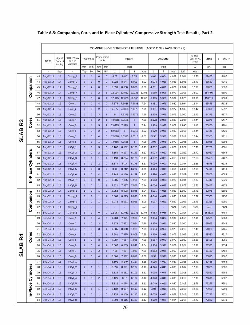
76
Table A.3: Companion, Core, and In‐Place Cylinders’ Compressive Strength Test Results, Part 2
CROSS-SECTIONAL
AREALOAD
mm mm mm mm in2 lbs.
- day - Top Bot Top Bot 1 2 3 Ave 1 2 Ave L/D Ave -
43 Aug-12-14 14 Comp_1 2 1 0 0 8.07 8.06 8.05 8.06 4.04 4.004 4.022 2.004 12.70 69455
44 Aug-12-14 14 Comp_2 2 1 0 0 8.022 8.044 8.003 8.02 4.024 4.018 4.021 1.995 12.70 66560
45 Aug-12-14 14 Comp_3 2 2 0 0 8.039 8.058 8.076 8.06 4.031 4.011 4.021 2.004 12.70 69880
46 Aug-12-14 14 Comp_4 2 1 2 1 12.094 12.063 12.031 12.06 5.959 5.998 5.979 2.018 28.07 154400
47 Aug-12-14 14 Comp_5 2 0 0 1 12.125 12.063 12.063 12.08 5.995 5.969 5.982 2.020 28.10 159315
48 Aug-12-14 16 Core_1 1 0 4 0 7.875 7.9688 7.9688 7.94 3.981 3.979 3.980 1.994 12.44 63855
49 Aug-12-14 16 Core_2 0 0 2 0 7.875 7.9063 7.9375 7.91 3.981 3.972 3.977 1.988 12.42 63300
50 Aug-12-14 16 Core_3 0 1 3 1 8 7.9375 7.9375 7.96 3.979 3.979 3.979 2.000 12.43 64375
51 Aug-12-14 16 Core_4 1 1 2 1 7.9688 7.9688 8 7.98 3.978 3.981 3.980 2.005 12.44 67375
52 Aug-12-14 16 Core_5 1 1 5 2 7.9375 7.875 8 7.94 3.979 3.977 3.978 1.995 12.43 70860
53 Aug-12-14 16 Core_6 0 0 2 0 8.0313 8 8.0313 8.02 3.979 3.981 3.980 2.015 12.44 67445
54 Aug-12-14 16 Core_7 2 0 4 0 7.9688 8.0313 8.0313 8.01 3.98 3.981 3.981 2.012 12.44 73560
55 Aug-12-14 16 Core_8 0 1 1 0 7.9688 7.9688 8 7.98 3.98 3.978 3.979 2.005 12.43 67085
56 Aug-12-14 16 InCyl_1 2 1 3 0 8.162 8.102 8.123 8.13 4.002 4.039 4.021 2.022 12.70 80760
57 Aug-12-14 16 InCyl_2 1 2 2 0 8.154 8.197 8.153 8.17 4.023 4.027 4.025 2.029 12.72 81020
58 Aug-12-14 16 InCyl_3 3 1 1 1 8.198 8.204 8.178 8.19 4.002 4.035 4.019 2.039 12.68 81455
59 Aug-12-14 16 InCyl_4 1 1 2 0 8.174 8.17 8.175 8.17 4.019 4.007 4.013 2.037 12.65 78845
60 Aug-12-14 16 InCyl_5 1 0 3 0 8.19 8.212 8.222 8.21 4.014 4.014 4.014 2.045 12.65 77415
61 Aug-12-14 16 InCyl_6 2 0 4 0 8.148 8.169 8.189 8.17 3.996 4.056 4.026 2.029 12.73 77505
62 Aug-12-14 16 InCyl_7 0 1 0 0 7.986 7.986 7.985 7.99 4.013 4.038 4.026 1.984 12.73 80440
63 Aug-12-14 16 InCyl_8 0 0 1 1 7.921 7.927 7.966 7.94 4.004 4.042 4.023 1.973 12.71 78465
64 Sep-02-14 14 Comp_1 1 2 1 0 8.058 8.023 8.045 8.04 4.031 4.015 4.023 1.999 12.71 69975
65 Sep-02-14 14 Comp_2 2 1 1 1 8.068 8.073 8.096 8.08 4.044 4.027 4.036 2.002 12.79 73550
66 Sep-02-14 14 Comp_3 2 2 1 0 8.073 8.081 8.086 8.08 4.037 4.021 4.029 2.005 12.75 67315
67 Sep-02-14 14 Comp_4 - - - - - - - NaN - - NaN NaN NaN NaN
68 Sep-02-14 14 Comp_5 1 1 0 0 12.063 12.031 12.031 12.04 5.953 5.986 5.970 2.017 27.99 153610
69 Sep-04-14 16 Core_1 1 0 4 0 7.904 7.921 7.954 7.93 3.984 3.884 3.934 2.015 12.16 67585
70 Sep-04-14 16 Core_2 1 0 3 0 7.978 7.952 7.954 7.96 3.979 3.981 3.980 2.000 12.44 68955
71 Sep-04-14 16 Core_3 2 0 3 1 7.985 8.008 7.985 7.99 3.984 3.962 3.973 2.012 12.40 64028
72 Sep-04-14 16 Core_4 0 0 1 1 7.981 7.975 8.009 7.99 3.966 3.988 3.977 2.009 12.42 68530
73 Sep-04-14 16 Core_5 1 0 3 0 7.987 7.957 7.986 7.98 3.967 3.973 3.970 2.009 12.38 61405
74 Sep-04-14 16 Core_6 1 0 4 1 8.067 8.005 8.042 8.04 3.966 3.976 3.971 2.024 12.38 68535
75 Sep-04-14 16 Core_7 1 0 3 1 7.98 7.987 7.967 7.98 3.983 3.936 3.960 2.015 12.31 67130
76 Sep-04-14 16 Core_8 1 0 4 1 8.006 7.992 8.011 8.00 3.99 3.976 3.983 2.009 12.46 66815
77 Sep-04-14 16 InCyl_1 - - - - 8.191 8.149 8.117 8.15 4.036 4.017 4.027 2.025 12.73 69435
78 Sep-04-14 16 InCyl_2 1 1 1 0 8.095 8.091 8.107 8.10 4.026 4.043 4.035 2.007 12.78 71665
79 Sep-04-14 16 InCyl_3 1 0 1 0 8.115 8.111 8.101 8.11 4.018 4.046 4.032 2.011 12.77 73860
80 Sep-04-14 16 InCyl_4 3 0 2 0 8.126 8.12 8.107 8.12 4.023 4.046 4.035 2.012 12.78 71615
81 Sep-04-14 16 InCyl_5 - - - - 8.132 8.078 8.115 8.11 4.049 4.011 4.030 2.012 12.76 76295
82 Sep-04-14 16 InCyl_6 2 1 1 2 8.132 8.107 8.113 8.12 4.04 4.018 4.029 2.015 12.75 73930
83 Sep-04-14 16 InCyl_7 1 0 1 0 8.124 8.109 8.113 8.12 4.009 4.035 4.022 2.018 12.70 70775
84 Sep-04-14 16 InCyl_8 - - - - 8.093 8.116 8.137 8.12 4.019 4.029 4.024 2.017 12.72 70880
STRENGTHDATE
Age of Conc at testing
GROUP/SAMPLE ID
NUMBER
RoughnessPerpendicul
arityHEIGHT DIAMETER
-
inch inch psi
SL
AB
R3
Co
mp
anio
n 5467
5241
5503
5500
5669
Co
res
5133
5097
5177
5417
5701
5421
5911
5395
In-P
lace
Cyl
ind
ers
6361
6368
6422
6234
6118
6088
6320
6173
SL
AB
R4
Co
mp
anio
n 5505
5750
5280
NaN
5489
Co
res
5560
5543
5165
5517
4961
5534
5452
5362
In-P
lace
Cyl
ind
ers
5453
5606
5785
5602
5981
5799
5571
5573
COMPRESSIVE STRENGTH TESTING (ASTM C 39 / AASHTO T 22)

77
Table A.3: Companion, Core, and In‐Place Cylinders’ Compressive Strength Test Results, Part 3
CROSS-SECTIONAL
AREALOAD
mm mm mm mm in2 lbs.
- day - Top Bot Top Bot 1 2 3 Ave 1 2 Ave L/D Ave -
85 Sep-16-14 14 Comp_1 2 1 2 1 8.0313 8.0313 8.0938 8.05 4.043 4.017 4.030 1.998 12.76 60375
86 Sep-16-14 14 Comp_2 2 0 2 1 8 8.0625 8.0313 8.03 4 3.9375 3.969 2.024 12.37 59350
87 Sep-16-14 14 Comp_3 1 0 4 1 7.9375 8.0625 8.25 8.08 3.9375 4 3.969 2.037 12.37 61205
88 Sep-16-14 14 Comp_4 1 1 1 1 12.063 12.25 12.25 12.19 6.0313 5.9688 6.000 2.031 28.27 130235
89 Sep-16-14 14 Comp_5 2 1 2 1 12.188 12.063 12.25 12.17 5.9375 6 5.969 2.038 27.98 129040
90 Sep-18-14 16 Core_1 2 1 3 2 7.846 7.767 7.798 7.80 3.993 3.987 3.990 1.956 12.50 60950
91 Sep-18-14 16 Core_2 2 3 3 1 7.878 8.004 8.007 7.96 3.974 3.994 3.984 1.999 12.47 57760
92 Sep-18-14 16 Core_3 2 2 3 2 8.11 8.039 8.079 8.08 3.978 3.979 3.979 2.030 12.43 56420
93 Sep-18-14 16 Core_4 3 2 4 3 8.093 8.087 7.993 8.06 3.978 3.976 3.977 2.026 12.42 55835
94 Sep-18-14 16 Core_5 1 2 4 1 8.031 7.986 8.107 8.04 3.981 3.983 3.982 2.019 12.45 56380
95 Sep-18-14 16 Core_6 0 0 1 1 8.05 8.049 8.04 8.05 3.977 3.979 3.978 2.023 12.43 54160
96 Sep-18-14 16 Core_7 1 1 3 2 8.088 8.039 8.036 8.05 3.979 3.986 3.983 2.022 12.46 56210
97 Sep-18-14 16 Core_8 2 1 3 2 7.945 7.983 7.975 7.97 3.987 3.991 3.989 1.997 12.50 57795
98 Sep-18-14 16 InCyl_1 0 2 0 3 8.16 8.202 8.109 8.16 4.023 4.012 4.018 2.030 12.68 66470
99 Sep-18-14 16 InCyl_2 1 2 2 3 8.137 8.13 8.152 8.14 4.034 4.033 4.034 2.018 12.78 64140
100 Sep-18-14 16 InCyl_3 2 0 1 3 8.056 8.025 8.072 8.05 4.03 4.036 4.033 1.996 12.77 63535
101 Sep-18-14 16 InCyl_4 1 3 2 3 8.105 8.118 8.112 8.11 4.014 4.008 4.011 2.022 12.64 64275
102 Sep-18-14 16 InCyl_5 2 0 2 1 7.98 8.004 8.034 8.01 4.042 4.039 4.041 1.981 12.82 63395
103 Sep-18-14 16 InCyl_6 1 3 2 3 8.079 8.071 8.106 8.09 3.994 4.065 4.030 2.007 12.75 62620
104 Sep-18-14 16 InCyl_7 0 3 1 2 8.182 8.161 8.156 8.17 4.018 4.019 4.019 2.032 12.68 65400
105 Sep-18-14 16 InCyl_8 2 0 1 3 8.058 8.044 8.028 8.04 4.045 3.976 4.011 2.006 12.63 64040
106 Oct-21-14 14 Comp_1 3 2 1 0 8 8.0313 8.0313 8.02 4.03 4.004 4.017 1.997 12.67 74760
107 Oct-21-14 14 Comp_2 2 1 2 0 8 7.9688 8 7.99 3.989 4.004 3.997 1.999 12.54 75455
108 Oct-21-14 14 Comp_3 4 2 1 0 8.25 8.125 8.0938 8.16 3.967 3.962 3.965 2.057 12.34 74930
109 Oct-21-14 14 Comp_4 3 1 2 1 11.969 12.125 12 12.03 5.948 5.893 5.921 2.032 27.53 167640
110 Oct-21-14 14 Comp_5 1 1 4 1 12.125 12.063 12.063 12.08 5.959 5.933 5.946 2.032 27.77 161465
111 Oct-23-14 16 Core_1 1 0 2 1 8.0313 8 8.0313 8.02 3.982 3.984 3.983 2.014 12.46 77120
112 Oct-23-14 16 Core_2 0 0 3 0 7.9688 8 7.9688 7.98 3.986 3.987 3.987 2.002 12.48 76200
113 Oct-23-14 16 Core_3 1 0 3 0 7.875 7.875 7.9375 7.90 3.987 3.988 3.988 1.980 12.49 70255
114 Oct-23-14 16 Core_4 1 0 2 1 7.9688 8.0313 7.9375 7.98 3.984 3.989 3.987 2.002 12.48 70450
115 Oct-23-14 16 Core_5 2 0 2 1 8.0625 7.9688 8.0313 8.02 3.984 3.985 3.985 2.013 12.47 70880
116 Oct-23-14 16 Core_6 0 0 3 1 8 8 8 8.00 3.985 3.988 3.987 2.007 12.48 73670
117 Oct-23-14 16 Core_7 0 0 1 0 8.0313 8 8.0313 8.02 3.989 3.989 3.989 2.011 12.50 75610
118 Oct-23-14 16 Core_8 0 0 3 0 7.9688 8.0313 8.0625 8.02 3.987 3.989 3.988 2.011 12.49 74530
119 Oct-23-14 16 InCyl_1 2 0 1.5 0.1 8.0625 8.0938 8.125 8.09 4.023 4.036 4.030 2.009 12.75 75605
120 Oct-23-14 16 InCyl_2 0.5 0 1.5 0 8.0313 8.0625 8.0625 8.05 4 4 4.000 2.013 12.57 77435
121 Oct-23-14 16 InCyl_3 1.5 0 2.5 0 8 8.0313 8.0313 8.02 4.057 3.985 4.021 1.995 12.70 81660
122 Oct-23-14 16 InCyl_4 2 0 2.5 0 8.0938 8.125 8.125 8.11 4.041 4.014 4.028 2.015 12.74 80035
123 Oct-23-14 16 InCyl_5 3 0 3 0 8.1563 8.1563 8.1563 8.16 4 4 4.000 2.039 12.57 75575
124 Oct-23-14 16 InCyl_6 1.5 0 1 0 8.0625 8.0625 8.0938 8.07 4.023 4.036 4.030 2.003 12.75 78760
125 Oct-23-14 16 InCyl_7 1.5 1 3 0 8.125 8.0625 8.125 8.10 4.051 4.007 4.029 2.011 12.75 76130
126 Oct-23-14 16 InCyl_8 0.5 0 0 0 8 8 8 8.00 4.008 4.018 4.013 1.994 12.65 76625
STRENGTHDATE
Age of Conc at testing
GROUP/SAMPLE ID
NUMBER
RoughnessPerpendicul
arityHEIGHT DIAMETER
-
inch inch psi
SL
AB
R5
Co
mp
anio
n 4733
4798
4948
4606
4612
Co
res
4875
4633
4538
4495
4527
4358
4512
4625
In-P
lace
Cyl
ind
ers
5244
5020
4974
5087
4944
4910
5157
5069
SL
AB
R6
Co
mp
anio
n 5899
6015
6070
6089
5815
Co
res
6190
6105
5626
5644
5684
5902
6050
5967
In-P
lace
Cyl
ind
ers
5929
6162
6431
6282
6014
6176
5971
6058
COMPRESSIVE STRENGTH TESTING (ASTM C 39 / AASHTO T 22)

78
Table A.3: Companion, Core, and In‐Place Cylinders’ Compressive Strength Test Results, Part 4
CROSS-SECTIONAL
AREALOAD
mm mm mm mm in2 lbs.
- day - Top Bot Top Bot 1 2 3 Ave 1 2 Ave L/D Ave -
127 Oct-7-14 14 Comp_1 1 0 2 1 8.09 8.092 8.082 8.09 4.02 4.034 4.027 2.008 12.74 70910
128 Oct-7-14 14 Comp_2 1 0 1 2 8.083 8.11 8.13 8.11 3.999 4.065 4.032 2.011 12.77 70720
129 Oct-7-14 14 Comp_3 1 0 2 0 8.07 8.088 8.093 8.08 4.054 4.042 4.048 1.997 12.87 65225
130 Oct-7-14 14 Comp_4 1 0 1 0 12.125 12.188 12.125 12.15 5.97 5.984 5.977 2.032 28.06 167290
131 Oct-7-14 14 Comp_5 2 0 3 1 12.125 12.125 12.125 12.13 5.966 5.946 5.956 2.036 27.86 165120
132 Oct-9-14 16 Core_1 0 0 0 0 7.984 8 8.004 8.00 3.989 3.987 3.988 2.005 12.49 79370
133 Oct-9-14 16 Core_2 0 0 1 0 7.941 7.938 7.97 7.95 3.991 3.987 3.989 1.993 12.50 71970
134 Oct-9-14 16 Core_3 0 3 2 1 8.038 8.065 8.003 8.04 3.99 3.986 3.988 2.015 12.49 75015
135 Oct-9-14 16 Core_4 0 1 1 2 7.991 7.999 7.991 7.99 3.985 3.985 3.985 2.006 12.47 78195
136 Oct-9-14 16 Core_5 0 1 0 0 8.007 8.006 7.983 8.00 3.989 3.985 3.987 2.006 12.48 77825
137 Oct-9-14 16 Core_6 1 0 0 0 8.013 8.02 8.106 8.05 3.99 3.989 3.990 2.017 12.50 75785
138 NaN NaN NaN
139 Oct-9-14 16 Core_8 0 1 2 2 8.01 8.069 8.03 8.04 3.984 3.987 3.986 2.016 12.48 72990
140 Oct-9-14 16 InCyl_1 0 0 0 1 8.008 8.01 7.946 7.99 4 4 4.000 1.997 12.57 70155
141 Oct-9-14 16 InCyl_2 1 0 0 2 8.065 8.086 8.008 8.05 4 4 4.000 2.013 12.57 66105
142 Oct-9-14 16 InCyl_3 1 1 1 2 8.112 8.096 8.095 8.10 4 4 4.000 2.025 12.57 68455
143 Oct-9-14 16 InCyl_4 1 0 1 1 7.942 7.962 7.954 7.95 4 4 4.000 1.988 12.57 67895
144 Oct-9-14 16 InCyl_5 1 0 1 1 7.975 7.986 7.962 7.97 4 4 4.000 1.994 12.57 70165
145 Oct-9-14 16 InCyl_6 2 0 0 2 8.052 8.266 7.843 8.05 4 4 4.000 2.013 12.57 67655
146 Oct-9-14 16 InCyl_7 3 0 0 2 7.975 7.986 7.962 7.97 4 4 4.000 1.994 12.57 72695
147 Oct-9-14 16 InCyl_8 1 3 0 3 7.919 7.951 7.917 7.93 4 4 4.000 1.982 12.57 61380
148 Oct-14-14 14 Comp_1 2 0 1 0 8.1 8.056 8.129 8.10 4.049 4.062 4.056 1.996 12.92 75095
149 Oct-14-14 14 Comp_2 2 0 4 0 8.059 8.099 8.152 8.10 4.016 4.032 4.024 2.014 12.72 74765
150 Oct-14-14 14 Comp_3 3 0 1 1 8.129 8.119 8.142 8.13 4.064 4.054 4.059 2.003 12.94 74810
151 Oct-14-14 14 Comp_4 3 1 3 0 12.125 12.063 12.125 12.10 5.963 6.002 5.983 2.023 28.11 153200
152 Oct-14-14 14 Comp_5 2 0 4 1 11.938 12.125 12.125 12.06 5.959 6.035 5.997 2.011 28.25 156850
153 Oct-16-14 16 Core_1 0 2 0 0 8.052 8.036 8.053 8.05 3.997 3.994 3.996 2.014 12.54 73470
154 Oct-16-14 16 Core_2 0 2 0 0 8.005 8.08 8.062 8.05 3.985 3.986 3.986 2.020 12.48 59220
155 Oct-16-14 16 Core_3 0 1 0 0 8.024 7.986 8.042 8.02 3.992 3.993 3.993 2.008 12.52 68465
156 Oct-16-14 16 Core_4 0 1 0 0 8.086 8.053 8.116 8.09 3.982 3.986 3.984 2.029 12.47 65430
157 Oct-16-14 16 Core_5 0 3 0 0 8.05 8.025 8.026 8.03 3.992 3.994 3.993 2.012 12.52 66875
158 Oct-16-14 16 Core_6 0 0 0 2 8.043 8.026 8.009 8.03 3.994 3.992 3.993 2.010 12.52 69330
159 Oct-16-14 16 Core_7 0 0 0 0 8.132 8.041 8.066 8.08 3.992 3.987 3.990 2.025 12.50 67220
160 Oct-16-14 16 Core_8 0 2 0 0 8.012 8.013 7.994 8.01 3.989 3.985 3.987 2.008 12.48 70790
161 Oct-16-14 16 InCyl_1 0 1 0 2 8.096 8.063 8.044 8.07 4.022 4.033 4.028 2.003 12.74 71235
162 Oct-16-14 16 InCyl_2 0 1 0 2 8.117 8.142 8.179 8.15 4.027 4.036 4.032 2.021 12.77 73660
163 Oct-16-14 16 InCyl_3 0 2 0 3 8.189 8.139 8.176 8.17 4.012 4.035 4.024 2.030 12.71 78015
164 Oct-16-14 16 InCyl_4 0 1 0 2 8.033 8.087 8.061 8.06 4.052 3.994 4.023 2.004 12.71 77350
165 Oct-16-14 16 InCyl_5 0 2 1 2 8.124 8.202 8.168 8.16 4.047 4.014 4.031 2.026 12.76 73475
166 Oct-16-14 16 InCyl_6 0 2 0 3 8.038 8.063 8.139 8.08 4.04 4.013 4.027 2.007 12.73 75190
167 Oct-16-14 16 InCyl_7 0 1 0 2 8.109 8.052 8.11 8.09 4.034 4.023 4.029 2.008 12.75 77700
168 Oct-16-14 16 InCyl_8 0 1 0 2 8.165 8.136 8.11 8.14 4.009 4.065 4.037 2.016 12.80 79540
STRENGTHDATE
Age of Conc at testing
GROUP/SAMPLE ID
NUMBER
RoughnessPerpendicul
arityHEIGHT DIAMETER
-
inch inch psi
SL
AB
R7
Co
mp
anio
n 5567
5539
5068
5962
5927
Co
res
6354
5759
6005
6269
6234
6063
NaN
5851
In-P
lace
Cyl
ind
ers
5583
5260
5447
5403
5584
5384
5785
4884
SL
AB
R8
Co
mp
anio
n 5813
5879
5781
5450
5553
Co
res
5860
4747
5469
5249
5340
5536
5377
5670
In-P
lace
Cyl
ind
ers
5592
5770
6136
6085
5759
5905
6096
6214
COMPRESSIVE STRENGTH TESTING (ASTM C 39 / AASHTO T 22)
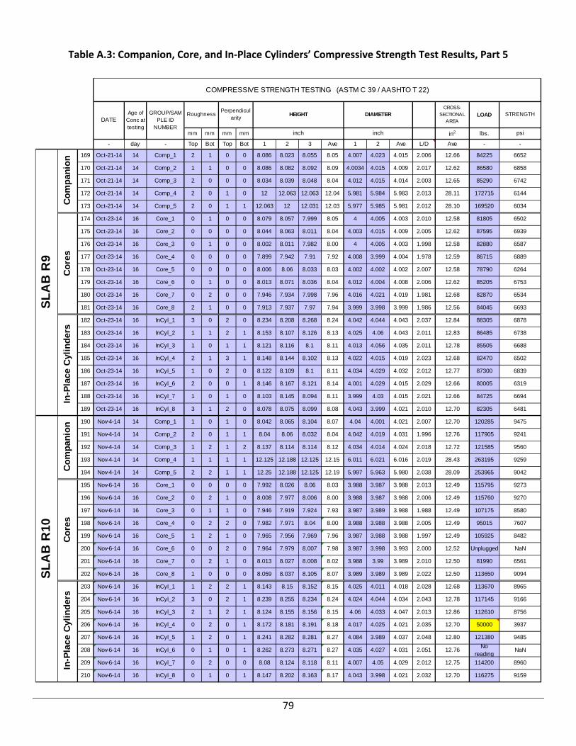
79
Table A.3: Companion, Core, and In‐Place Cylinders’ Compressive Strength Test Results, Part 5
CROSS-SECTIONAL
AREALOAD
mm mm mm mm in2 lbs.
- day - Top Bot Top Bot 1 2 3 Ave 1 2 Ave L/D Ave -
169 Oct-21-14 14 Comp_1 2 1 0 0 8.086 8.023 8.055 8.05 4.007 4.023 4.015 2.006 12.66 84225
170 Oct-21-14 14 Comp_2 1 1 0 0 8.086 8.082 8.092 8.09 4.0034 4.015 4.009 2.017 12.62 86580
171 Oct-21-14 14 Comp_3 2 0 0 0 8.034 8.039 8.048 8.04 4.012 4.015 4.014 2.003 12.65 85290
172 Oct-21-14 14 Comp_4 2 0 1 0 12 12.063 12.063 12.04 5.981 5.984 5.983 2.013 28.11 172715
173 Oct-21-14 14 Comp_5 2 0 1 1 12.063 12 12.031 12.03 5.977 5.985 5.981 2.012 28.10 169520
174 Oct-23-14 16 Core_1 0 1 0 0 8.079 8.057 7.999 8.05 4 4.005 4.003 2.010 12.58 81805
175 Oct-23-14 16 Core_2 0 0 0 0 8.044 8.063 8.011 8.04 4.003 4.015 4.009 2.005 12.62 87595
176 Oct-23-14 16 Core_3 0 1 0 0 8.002 8.011 7.982 8.00 4 4.005 4.003 1.998 12.58 82880
177 Oct-23-14 16 Core_4 0 0 0 0 7.899 7.942 7.91 7.92 4.008 3.999 4.004 1.978 12.59 86715
178 Oct-23-14 16 Core_5 0 0 0 0 8.006 8.06 8.033 8.03 4.002 4.002 4.002 2.007 12.58 78790
179 Oct-23-14 16 Core_6 0 1 0 0 8.013 8.071 8.036 8.04 4.012 4.004 4.008 2.006 12.62 85205
180 Oct-23-14 16 Core_7 0 2 0 0 7.946 7.934 7.998 7.96 4.016 4.021 4.019 1.981 12.68 82870
181 Oct-23-14 16 Core_8 2 1 0 0 7.913 7.937 7.97 7.94 3.999 3.998 3.999 1.986 12.56 84045
182 Oct-23-14 16 InCyl_1 3 0 2 0 8.234 8.208 8.268 8.24 4.042 4.044 4.043 2.037 12.84 88305
183 Oct-23-14 16 InCyl_2 1 1 2 1 8.153 8.107 8.126 8.13 4.025 4.06 4.043 2.011 12.83 86485
184 Oct-23-14 16 InCyl_3 1 0 1 1 8.121 8.116 8.1 8.11 4.013 4.056 4.035 2.011 12.78 85505
185 Oct-23-14 16 InCyl_4 2 1 3 1 8.148 8.144 8.102 8.13 4.022 4.015 4.019 2.023 12.68 82470
186 Oct-23-14 16 InCyl_5 1 0 2 0 8.122 8.109 8.1 8.11 4.034 4.029 4.032 2.012 12.77 87300
187 Oct-23-14 16 InCyl_6 2 0 0 1 8.146 8.167 8.121 8.14 4.001 4.029 4.015 2.029 12.66 80005
188 Oct-23-14 16 InCyl_7 1 0 1 0 8.103 8.145 8.094 8.11 3.999 4.03 4.015 2.021 12.66 84725
189 Oct-23-14 16 InCyl_8 3 1 2 0 8.078 8.075 8.099 8.08 4.043 3.999 4.021 2.010 12.70 82305
190 Nov-4-14 14 Comp_1 1 0 1 0 8.042 8.065 8.104 8.07 4.04 4.001 4.021 2.007 12.70 120285
191 Nov-4-14 14 Comp_2 2 0 1 1 8.04 8.06 8.032 8.04 4.042 4.019 4.031 1.996 12.76 117905
192 Nov-4-14 14 Comp_3 1 2 1 2 8.137 8.114 8.114 8.12 4.034 4.014 4.024 2.018 12.72 121585
193 Nov-4-14 14 Comp_4 1 1 1 1 12.125 12.188 12.125 12.15 6.011 6.021 6.016 2.019 28.43 263195
194 Nov-4-14 14 Comp_5 2 2 1 1 12.25 12.188 12.125 12.19 5.997 5.963 5.980 2.038 28.09 253965
195 Nov-6-14 16 Core_1 0 0 0 0 7.992 8.026 8.06 8.03 3.988 3.987 3.988 2.013 12.49 115795
196 Nov-6-14 16 Core_2 0 2 1 0 8.008 7.977 8.006 8.00 3.988 3.987 3.988 2.006 12.49 115760
197 Nov-6-14 16 Core_3 0 1 1 0 7.946 7.919 7.924 7.93 3.987 3.989 3.988 1.988 12.49 107175
198 Nov-6-14 16 Core_4 0 2 2 0 7.982 7.971 8.04 8.00 3.988 3.988 3.988 2.005 12.49 95015
199 Nov-6-14 16 Core_5 1 2 1 0 7.965 7.956 7.969 7.96 3.987 3.988 3.988 1.997 12.49 105925
200 Nov-6-14 16 Core_6 0 0 2 0 7.964 7.979 8.007 7.98 3.987 3.998 3.993 2.000 12.52 Unplugged
201 Nov-6-14 16 Core_7 0 2 1 0 8.013 8.027 8.008 8.02 3.988 3.99 3.989 2.010 12.50 81990
202 Nov-6-14 16 Core_8 1 0 0 0 8.059 8.037 8.105 8.07 3.989 3.989 3.989 2.022 12.50 113650
203 Nov-6-14 16 InCyl_1 1 2 2 1 8.143 8.15 8.152 8.15 4.025 4.011 4.018 2.028 12.68 113670
204 Nov-6-14 16 InCyl_2 3 0 2 1 8.239 8.255 8.234 8.24 4.024 4.044 4.034 2.043 12.78 117145
205 Nov-6-14 16 InCyl_3 2 1 2 1 8.124 8.155 8.156 8.15 4.06 4.033 4.047 2.013 12.86 112610
206 Nov-6-14 16 InCyl_4 0 2 0 1 8.172 8.181 8.191 8.18 4.017 4.025 4.021 2.035 12.70 50000
207 Nov-6-14 16 InCyl_5 1 2 0 1 8.241 8.282 8.281 8.27 4.084 3.989 4.037 2.048 12.80 121380
208 Nov-6-14 16 InCyl_6 0 1 0 1 8.262 8.273 8.271 8.27 4.035 4.027 4.031 2.051 12.76No
reading
209 Nov-6-14 16 InCyl_7 0 2 0 0 8.08 8.124 8.118 8.11 4.007 4.05 4.029 2.012 12.75 114200
210 Nov-6-14 16 InCyl_8 0 1 0 1 8.147 8.202 8.163 8.17 4.043 3.998 4.021 2.032 12.70 116275
STRENGTHDATE
Age of Conc at testing
GROUP/SAMPLE ID
NUMBER
RoughnessPerpendicul
arityHEIGHT DIAMETER
-
inch inch psi
SL
AB
R9
Co
mp
anio
n 6652
6858
6742
6144
6034
Co
res
6502
6939
6587
6889
6264
6753
6534
6693
In-P
lace
Cyl
ind
ers
6878
6738
6688
6502
6839
6319
6694
6481
SL
AB
R10
Co
mp
anio
n 9475
9241
9560
9259
9042
Co
res
9273
9270
8580
7607
8482
NaN
6561
9094
In-P
lace
Cyl
ind
ers
8965
9166
8756
3937
9485
NaN
8960
9159
COMPRESSIVE STRENGTH TESTING (ASTM C 39 / AASHTO T 22)
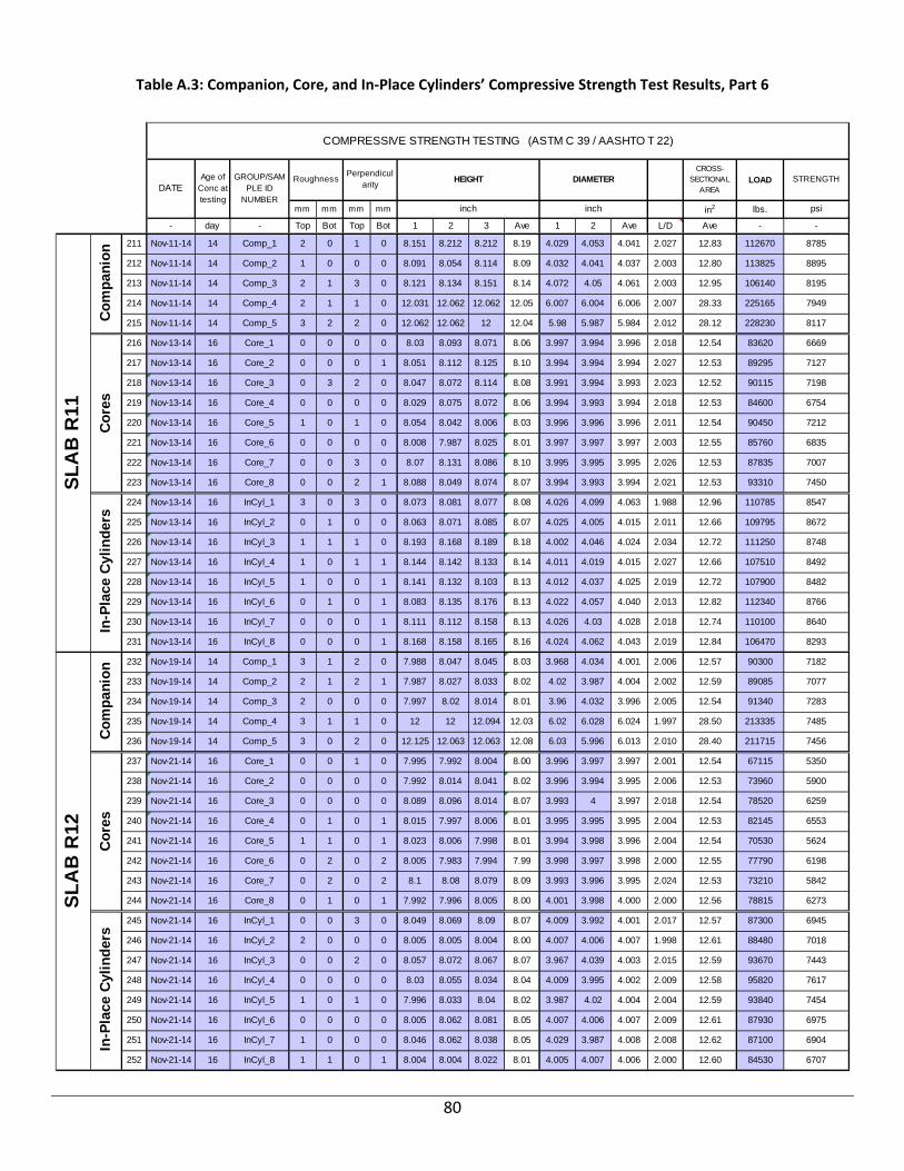
80
Table A.3: Companion, Core, and In‐Place Cylinders’ Compressive Strength Test Results, Part 6
CROSS-SECTIONAL
AREALOAD
mm mm mm mm in2 lbs.
- day - Top Bot Top Bot 1 2 3 Ave 1 2 Ave L/D Ave -
211 Nov-11-14 14 Comp_1 2 0 1 0 8.151 8.212 8.212 8.19 4.029 4.053 4.041 2.027 12.83 112670
212 Nov-11-14 14 Comp_2 1 0 0 0 8.091 8.054 8.114 8.09 4.032 4.041 4.037 2.003 12.80 113825
213 Nov-11-14 14 Comp_3 2 1 3 0 8.121 8.134 8.151 8.14 4.072 4.05 4.061 2.003 12.95 106140
214 Nov-11-14 14 Comp_4 2 1 1 0 12.031 12.062 12.062 12.05 6.007 6.004 6.006 2.007 28.33 225165
215 Nov-11-14 14 Comp_5 3 2 2 0 12.062 12.062 12 12.04 5.98 5.987 5.984 2.012 28.12 228230
216 Nov-13-14 16 Core_1 0 0 0 0 8.03 8.093 8.071 8.06 3.997 3.994 3.996 2.018 12.54 83620
217 Nov-13-14 16 Core_2 0 0 0 1 8.051 8.112 8.125 8.10 3.994 3.994 3.994 2.027 12.53 89295
218 Nov-13-14 16 Core_3 0 3 2 0 8.047 8.072 8.114 8.08 3.991 3.994 3.993 2.023 12.52 90115
219 Nov-13-14 16 Core_4 0 0 0 0 8.029 8.075 8.072 8.06 3.994 3.993 3.994 2.018 12.53 84600
220 Nov-13-14 16 Core_5 1 0 1 0 8.054 8.042 8.006 8.03 3.996 3.996 3.996 2.011 12.54 90450
221 Nov-13-14 16 Core_6 0 0 0 0 8.008 7.987 8.025 8.01 3.997 3.997 3.997 2.003 12.55 85760
222 Nov-13-14 16 Core_7 0 0 3 0 8.07 8.131 8.086 8.10 3.995 3.995 3.995 2.026 12.53 87835
223 Nov-13-14 16 Core_8 0 0 2 1 8.088 8.049 8.074 8.07 3.994 3.993 3.994 2.021 12.53 93310
224 Nov-13-14 16 InCyl_1 3 0 3 0 8.073 8.081 8.077 8.08 4.026 4.099 4.063 1.988 12.96 110785
225 Nov-13-14 16 InCyl_2 0 1 0 0 8.063 8.071 8.085 8.07 4.025 4.005 4.015 2.011 12.66 109795
226 Nov-13-14 16 InCyl_3 1 1 1 0 8.193 8.168 8.189 8.18 4.002 4.046 4.024 2.034 12.72 111250
227 Nov-13-14 16 InCyl_4 1 0 1 1 8.144 8.142 8.133 8.14 4.011 4.019 4.015 2.027 12.66 107510
228 Nov-13-14 16 InCyl_5 1 0 0 1 8.141 8.132 8.103 8.13 4.012 4.037 4.025 2.019 12.72 107900
229 Nov-13-14 16 InCyl_6 0 1 0 1 8.083 8.135 8.176 8.13 4.022 4.057 4.040 2.013 12.82 112340
230 Nov-13-14 16 InCyl_7 0 0 0 1 8.111 8.112 8.158 8.13 4.026 4.03 4.028 2.018 12.74 110100
231 Nov-13-14 16 InCyl_8 0 0 0 1 8.168 8.158 8.165 8.16 4.024 4.062 4.043 2.019 12.84 106470
232 Nov-19-14 14 Comp_1 3 1 2 0 7.988 8.047 8.045 8.03 3.968 4.034 4.001 2.006 12.57 90300
233 Nov-19-14 14 Comp_2 2 1 2 1 7.987 8.027 8.033 8.02 4.02 3.987 4.004 2.002 12.59 89085
234 Nov-19-14 14 Comp_3 2 0 0 0 7.997 8.02 8.014 8.01 3.96 4.032 3.996 2.005 12.54 91340
235 Nov-19-14 14 Comp_4 3 1 1 0 12 12 12.094 12.03 6.02 6.028 6.024 1.997 28.50 213335
236 Nov-19-14 14 Comp_5 3 0 2 0 12.125 12.063 12.063 12.08 6.03 5.996 6.013 2.010 28.40 211715
237 Nov-21-14 16 Core_1 0 0 1 0 7.995 7.992 8.004 8.00 3.996 3.997 3.997 2.001 12.54 67115
238 Nov-21-14 16 Core_2 0 0 0 0 7.992 8.014 8.041 8.02 3.996 3.994 3.995 2.006 12.53 73960
239 Nov-21-14 16 Core_3 0 0 0 0 8.089 8.096 8.014 8.07 3.993 4 3.997 2.018 12.54 78520
240 Nov-21-14 16 Core_4 0 1 0 1 8.015 7.997 8.006 8.01 3.995 3.995 3.995 2.004 12.53 82145
241 Nov-21-14 16 Core_5 1 1 0 1 8.023 8.006 7.998 8.01 3.994 3.998 3.996 2.004 12.54 70530
242 Nov-21-14 16 Core_6 0 2 0 2 8.005 7.983 7.994 7.99 3.998 3.997 3.998 2.000 12.55 77790
243 Nov-21-14 16 Core_7 0 2 0 2 8.1 8.08 8.079 8.09 3.993 3.996 3.995 2.024 12.53 73210
244 Nov-21-14 16 Core_8 0 1 0 1 7.992 7.996 8.005 8.00 4.001 3.998 4.000 2.000 12.56 78815
245 Nov-21-14 16 InCyl_1 0 0 3 0 8.049 8.069 8.09 8.07 4.009 3.992 4.001 2.017 12.57 87300
246 Nov-21-14 16 InCyl_2 2 0 0 0 8.005 8.005 8.004 8.00 4.007 4.006 4.007 1.998 12.61 88480
247 Nov-21-14 16 InCyl_3 0 0 2 0 8.057 8.072 8.067 8.07 3.967 4.039 4.003 2.015 12.59 93670
248 Nov-21-14 16 InCyl_4 0 0 0 0 8.03 8.055 8.034 8.04 4.009 3.995 4.002 2.009 12.58 95820
249 Nov-21-14 16 InCyl_5 1 0 1 0 7.996 8.033 8.04 8.02 3.987 4.02 4.004 2.004 12.59 93840
250 Nov-21-14 16 InCyl_6 0 0 0 0 8.005 8.062 8.081 8.05 4.007 4.006 4.007 2.009 12.61 87930
251 Nov-21-14 16 InCyl_7 1 0 0 0 8.046 8.062 8.038 8.05 4.029 3.987 4.008 2.008 12.62 87100
252 Nov-21-14 16 InCyl_8 1 1 0 1 8.004 8.004 8.022 8.01 4.005 4.007 4.006 2.000 12.60 84530
STRENGTHDATE
Age of Conc at testing
GROUP/SAMPLE ID
NUMBER
RoughnessPerpendicul
arityHEIGHT DIAMETER
-
inch inch psi
SL
AB
R11
Co
mp
anio
n 8785
8895
8195
7949
8117
Co
res
6669
7127
7198
6754
7212
6835
7007
7450
In-P
lace
Cyl
ind
ers
8547
8672
8748
8492
8482
8766
8640
8293
SL
AB
R12
Co
mp
anio
n 7182
7077
7283
7485
7456
Co
res
5350
5900
6259
6553
5624
6198
5842
6273
In-P
lace
Cyl
ind
ers
6945
7018
7443
7617
7454
6975
6904
6707
COMPRESSIVE STRENGTH TESTING (ASTM C 39 / AASHTO T 22)

81
Table A.3: Companion, Core, and In‐Place Cylinders’ Compressive Strength Test Results, Part 7
CROSS-SECTIONAL
AREALOAD
mm mm mm mm in2 lbs.
- day - Top Bot Top Bot 1 2 3 Ave 1 2 Ave L/D Ave - - -
253 Nov-18-14 14 Comp_1 1 4 2 2 8.073 8.032 8.071 8.06 4.029 4.021 4.025 2.002 12.72 39535 36 60
254 Nov-18-14 14 Comp_2 2 1 3 1 8.088 8.057 8.097 8.08 4.022 4.023 4.023 2.009 12.71 39595 37 60
255 Nov-18-14 14 Comp_3 2 2 0 0 8.025 8.041 8.02 8.03 4.036 4.014 4.025 1.995 12.72 37400 38 60
256 Nov-18-14 14 Comp_4 1 3 0 1 12.063 12.125 12.125 12.10 5.973 6.001 5.987 2.022 28.15 77760 25 60
257 Nov-18-14 14 Comp_5 2 2 0 2 12.031 12.031 12.063 12.04 6.015 6.012 6.014 2.002 28.40 83840 26 60
258 Nov-20-14 16 Core_1 1 0 2 0 8.046 8.027 8.007 8.03 3.992 3.99 3.991 2.011 12.51 37485 42 60
259 Nov-20-14 16 Core_2 1 0 3 0 8.002 8.066 8.038 8.04 3.991 3.996 3.994 2.012 12.53 36520 43 60
260 Nov-20-14 16 Core_3 1 0 2 0 7.985 8.013 8.022 8.01 3.998 3.989 3.994 2.005 12.53 33640 44 60
261 Nov-20-14 16 Core_4 0 0 0 3 7.975 8.052 8.038 8.02 3.989 3.989 3.989 2.011 12.50 35210 45 60
262 Nov-20-14 16 Core_5 0 0 3 0 8.019 7.95 7.945 7.97 3.993 3.99 3.992 1.997 12.51 36545 46 60
263 Nov-20-14 16 Core_6 0 0 2 0 8 8.046 8.045 8.03 3.998 3.991 3.995 2.010 12.53 36755 47 60
264 Nov-20-14 16 Core_7 1 0 1 0 7.98 7.982 7.989 7.98 3.991 3.998 3.995 1.999 12.53 33435 48 60
265 Nov-20-14 16 Core_8 0 0 2 0 8.055 8.058 8.02 8.04 3.99 3.988 3.989 2.017 12.50 35885 49 60
266 Nov-20-14 16 InCyl_1 1 0 0 0 8 8 7.982 7.99 4.004 3.991 3.998 2.000 12.55 37215 50 60
267 Nov-20-14 16 InCyl_2 0 0 0 0 7.905 7.912 7.907 7.91 4.004 3.984 3.994 1.980 12.53 35330 51 60
268 Nov-20-14 16 InCyl_3 2 0 0 0 8.02 8.039 8.059 8.04 3.985 4.008 3.997 2.012 12.54 35300 52 60
269 Nov-20-14 16 InCyl_4 0 0 0 0 7.959 7.966 7.963 7.96 4.006 4.012 4.009 1.986 12.62 39610 53 60
270 Nov-20-14 16 InCyl_5 0 0 1 0 8.009 8.07 8.063 8.05 4 3.999 4.000 2.012 12.56 36320 54 60
271 Nov-20-14 16 InCyl_6 1 0 0 0 8.028 8.001 7.997 8.01 4.003 3.992 3.998 2.003 12.55 37640 55 60
272 Nov-20-14 16 InCyl_7 1 0 1 1 8.021 8.036 8.025 8.03 4.017 4.002 4.010 2.002 12.63 39235 56 60
273 Nov-20-14 16 InCyl_8 2 0 1 1 8.006 7.999 7.996 8.00 4.009 3.993 4.001 2.000 12.57 37635 57 60
274 Nov-24-14 14 Comp_1 2 1 0 0 8.052 8.042 8.082 8.06 4.146 4.03 4.088 1.971 13.13 38880 75 60
275 Nov-24-14 14 Comp_2 3 1 2 0 8.007 8.089 8.11 8.07 4.029 4.015 4.022 2.006 12.70 37995 76 60
276 Nov-24-14 14 Comp_3 2 1 1 0 8.096 8.132 8.106 8.11 4.044 4.03 4.037 2.009 12.80 38140 77 60
277 Nov-24-14 14 Comp_4 2 0 1 1 12.125 12 12 12.04 6.005 5.996 6.001 2.007 28.28 85855 29 60
278 Nov-24-14 14 Comp_5 2 1 1 0 12.063 12.125 12.094 12.09 6.009 6.008 6.009 2.013 28.35 83225 30 60
279 Nov-26-14 16 Core_1 0 0 1 1 7.965 7.972 7.977 7.97 3.993 3.984 3.989 1.999 12.49 36420 1 60
280 Nov-26-14 16 Core_2 0 0 1 0 8.001 7.992 7.992 8.00 3.996 3.984 3.990 2.004 12.50 39445 2 60
281 Nov-26-14 16 Core_3 0 0 0 0 7.918 7.919 7.932 7.92 3.994 3.996 3.995 1.983 12.53 39295 3 60
282 Nov-26-14 16 Core_4 0 0 0 0 7.929 7.925 7.94 7.93 3.993 3.993 3.993 1.986 12.52 37505 4 60
283 Nov-26-14 16 Core_5 0 0 0 1 7.954 7.933 7.943 7.94 3.996 3.996 3.996 1.988 12.54 36005 5 60
284 Nov-26-14 16 Core_6 0 0 1 1 7.92 7.918 7.924 7.92 3.996 3.997 3.997 1.982 12.54 39805 6 60
285 Nov-26-14 16 Core_7 0 0 1 1 7.953 7.945 7.954 7.95 3.995 3.995 3.995 1.990 12.53 38275 7 60
286 Nov-26-14 16 Core_8 0 0 2 0 7.951 7.962 7.97 7.96 3.996 3.997 3.997 1.992 12.54 39410 8 60
287 Nov-26-14 16 InCyl_1 1 0 3 0 8.1 8.05 8.048 8.07 3.986 4.017 4.002 2.016 12.58 40220 9 60
288 Nov-26-14 16 InCyl_2 2 0 3 0 8.093 8.158 8.111 8.12 3.995 4.012 4.004 2.028 12.59 39160 10 60
289 Nov-26-14 16 InCyl_3 1 0 2 0 8.077 8.094 8.128 8.10 4.05 3.989 4.020 2.015 12.69 43165 11 60
290 Nov-26-14 16 InCyl_4 3 2 2 0 8.121 8.145 8.103 8.12 4.016 4.05 4.033 2.014 12.77 40230 12 60
291 Nov-26-14 16 InCyl_5 1 0 2 1 8.026 8.039 8.023 8.03 4.002 3.994 3.998 2.008 12.55 41095 13 60
292 Nov-26-14 16 InCyl_6 2 0 1 0 8.072 8.055 8.065 8.06 4.033 3.975 4.004 2.014 12.59 41770 14 60
293 Nov-26-14 16 InCyl_7 2 0 0 1 8.073 8.039 8.117 8.08 4.009 4 4.005 2.017 12.59 40720 15 60
294 Nov-26-14 16 InCyl_8 0 0 0 0 8.0625 8.0938 - 8.08 3.966 4.033 4.000 2.020 12.56 40205 16 60
STRENGTHDATE
Age of Conc at testing
GROUP/SAMPLE ID
NUMBER
RoughnessPerpendicul
arityHEIGHT DIAMETER
-
inch inch psi
PA
D D
UR
OM
ET
ER
PA
D U
SE
SL
AB
R13
Co
mp
an
ion 3107
3116
2939
2762
2952
Co
res
2996
2916
2686
2817
2921
2933
2668
2871
In-P
lace C
yli
nd
ers
2965
2820
2814
3138
2891
2999
3107
2993
SL
AB
R1
4
Co
mp
an
ion 2962
2991
2980
3036
2935
Co
res
2915
3155
3135
2995
2871
3173
3053
3142
In-P
lace C
yli
nd
ers
3198
3111
3402
3149
3274
3317
3233
3200
COMPRESSIVE STRENGTH TESTING (ASTM C 39 / AASHTO T 22)

82
Table A.3: Companion, Core, and In‐Place Cylinders’ Compressive Strength Test Results, Part 8
CROSS-SECTIONAL
AREALOAD
mm mm mm mm in2 lbs.
- day - Top Bot Top Bot 1 2 3 Ave 1 2 Ave L/D Ave -
316 Dec-08-14 14 Comp_1 1 2 0 1 8.03 8.008 8.025 8.02 4.014 3.989 4.002 2.004 12.58 34020
317 Dec-08-14 14 Comp_2 2 2 1 1 8.044 8.039 8.043 8.04 4.001 4.006 4.004 2.009 12.59 33405
318 Dec-08-14 14 Comp_3 1 1 0 1 8.005 8.033 8.06 8.03 4.028 4 4.014 2.001 12.65 33890
319 Dec-08-14 14 Comp_4 1 2 1 2 12.125 12.094 12.063 12.09 5.99 5.964 5.977 2.023 28.06 74860
320 Dec-08-14 14 Comp_5 - - - - 12.031 11.969 11.969 11.99 5.996 5.968 5.982 2.004 28.10 67230
321 Dec-08-14 16 Core_1 1 0 1 1 8.019 8.01 8.022 8.02 4.005 4 4.003 2.003 12.58 25775
322 Dec-08-14 16 Core_2 3 0 1 2 8.02 8.018 8.002 8.01 3.995 3.998 3.997 2.005 12.54 26320
323 Dec-08-14 16 Core_3 0 0 0 1 8.073 8.074 8.073 8.07 3.995 3.994 3.995 2.021 12.53 25370
324 Dec-08-14 16 Core_4 3 0 0 0 7.996 8.004 7.99 8.00 4.001 3.996 3.999 2.000 12.56 23685
325 Dec-08-14 16 Core_5 0 0 3 1 7.984 7.994 7.988 7.99 3.994 3.997 3.996 1.999 12.54 26430
326 Dec-08-14 16 Core_6 1 0 3 0 8.016 8.004 8.015 8.01 3.999 3.999 3.999 2.003 12.56 27675
327 Dec-08-14 16 Core_7 0 0 1 1 8.081 8.06 8.067 8.07 3.997 4 3.999 2.018 12.56 26795
328 Dec-08-14 16 Core_8 0 1 1 2 8.041 8.032 8.04 8.04 3.999 4.004 4.002 2.009 12.58 27465
329 Dec-08-14 16 InCyl_1 2 0 2 0 8.059 8.008 8.038 8.04 4.002 4.005 4.004 2.007 12.59 31055
330 Dec-08-14 16 InCyl_2 1 2 2 0 8.013 8.04 8.041 8.03 3.977 4.029 4.003 2.006 12.59 32910
331 Dec-08-14 16 InCyl_3 3 0 1 0 8.013 8.017 8.019 8.02 3.993 4.011 4.002 2.003 12.58 31560
332 Dec-08-14 16 InCyl_4 2 0 1 0 8.1 8.093 8.091 8.09 3.991 4.016 4.004 2.022 12.59 33195
333 Dec-08-14 16 InCyl_5 2 0 1 0 8.013 8.029 8.055 8.03 4.002 4.024 4.013 2.002 12.65 32650
334 Dec-08-14 16 InCyl_6 2 0 1 1 8.022 8.011 8.028 8.02 3.987 4.018 4.003 2.004 12.58 33670
335 Dec-08-14 16 InCyl_7 1 0 1 0 8.043 8.108 8.06 8.07 3.997 4.024 4.011 2.012 12.63 35375
336 Dec-08-14 16 InCyl_8 1 0 2 0 8.044 8.069 8.115 8.08 4.035 4.017 4.026 2.006 12.73 35235
337 Feb-04-15 14 Comp_1 1 0 0 0 8 8 8 8.00 3.9688 3.9375 3.953 2.024 12.27 44245
338 Feb-04-15 14 Comp_2 1 1 1 0 8 7.9688 7.9375 7.97 3.9375 3.9375 3.938 2.024 12.18 43430
339 Feb-04-15 14 Comp_3 1 0 1 1 8 7.9688 8 7.99 4 3.9375 3.969 2.013 12.37 40820
340 Feb-04-15 14 Comp_4 2 0 0 1 12.125 12.125 12.094 12.11 5.9688 6 5.984 2.024 28.13 95890
341 Feb-04-15 14 Comp_5 2 0 2 0 12.25 12.125 12 12.13 6 5.9688 5.984 2.026 28.13 93770
342 Feb-06-15 16 Core_1 1 0 0 0 8 7.9688 7.9688 7.98 4 4 4.000 1.995 12.57 34610
343 Feb-06-15 16 Core_2 1 0 1 0 7.9688 8 8 7.99 3.9688 3.9688 3.969 2.013 12.37 39415
344 Feb-06-15 16 Core_3 1 0 1 0 8 8 7.9688 7.99 4 4 4.000 1.997 12.57 38440
345 Feb-06-15 16 Core_4 1 0 2 0 8 7.9375 7.9375 7.96 3.969 3.9688 3.969 2.005 12.37 38340
346 Feb-06-15 16 Core_5 1 0 1 0 7.9375 8 7.9688 7.97 3.969 3.9688 3.969 2.008 12.37 36460
347 Feb-06-15 16 Core_6 1 0 0 0 7.9375 7.9375 7.9375 7.94 4 3.9688 3.984 1.992 12.47 36580
348 Feb-06-15 16 Core_7 1 0 1 0 8.125 8.125 7.9688 8.07 3.969 3.9688 3.969 2.034 12.37 33565
349 Feb-06-15 16 Core_8 1 0 1 0 7.9688 7.9688 8 7.98 4 3.9688 3.984 2.003 12.47 37675
350 Feb-06-15 16 InCyl_1 1 0 0 0 8.0625 8.0313 8.0625 8.05 4 4 4.000 2.013 12.57 46170
351 Feb-06-15 16 InCyl_2 1 0 0 0 8.0313 8.0313 8 8.02 4 4 4.000 2.005 12.57 45580
352 Feb-06-15 16 InCyl_3 2 0 1 0 8.0313 8.0625 8.0313 8.04 4 4 4.000 2.010 12.57 47440
353 Feb-06-15 16 InCyl_4 2 0 2 0 8.0313 8.0313 8.0625 8.04 4.0313 3.9688 4.000 2.010 12.57 44670
354 Feb-06-15 16 InCyl_5 1 0 1 0 8.0313 7.9688 8.0625 8.02 4 3.9688 3.984 2.013 12.47 46110
355 Feb-06-15 16 InCyl_6 1 0 2 0 8 8.0313 8.0625 8.03 4 4 4.000 2.008 12.57 45900
356 Feb-06-15 16 InCyl_7 2 0 2 0 8.0625 8.0313 8.0625 8.05 3.9688 4 3.984 2.021 12.47 45065
357 Feb-06-15 16 InCyl_8 0 0 0 1 8 8 8 8.00 4 4 4.000 2.000 12.57 44240
STRENGTHDATE
Age of Conc at testing
GROUP/SAMPLE ID
NUMBER
RoughnessPerpendicul
arityHEIGHT DIAMETER
-
inch inch psi
SL
AB
R16
Co
mp
anio
n 2705
2654
2678
2668
2392
Co
res
2049
2098
2024
1886
2108
2203
2134
2184
In-P
lace
Cyl
ind
ers 2467
2615
2509
2637
2581
2676
2800
2768
SL
AB
R15
B
Co
mp
anio
n
3605
3567
3300
3409
3334
Co
res
2754
3186
3059
3099
2947
2934
2713
3022
In-P
lace
Cyl
ind
ers
3674
3627
3775
3555
3698
3653
3614
3521
COMPRESSIVE STRENGTH TESTING (ASTM C 39 / AASHTO T 22)
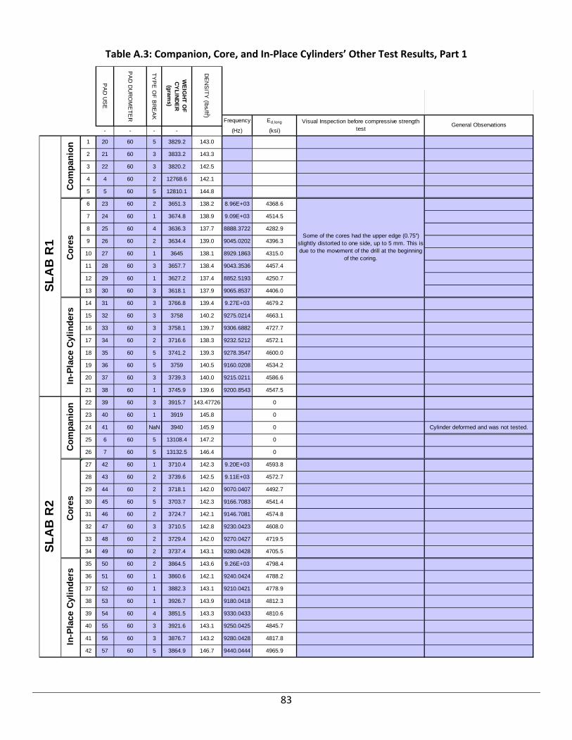
83
Table A.3: Companion, Core, and In‐Place Cylinders’ Other Test Results, Part 1
Frequency Ed,long
- - - - (Hz) (ksi)
1 20 60 5 3829.2 143.0
2 21 60 3 3833.2 143.3
3 22 60 3 3820.2 142.5
4 4 60 2 12768.6 142.1
5 5 60 5 12810.1 144.8
6 23 60 2 3651.3 138.2 8.96E+03 4368.6
7 24 60 1 3674.8 138.9 9.09E+03 4514.5
8 25 60 4 3636.3 137.7 8888.3722 4282.9
9 26 60 2 3634.4 139.0 9045.0202 4396.3
10 27 60 1 3645 138.1 8929.1863 4315.0
11 28 60 3 3657.7 138.4 9043.3536 4457.4
12 29 60 1 3627.2 137.4 8852.5193 4250.7
13 30 60 3 3618.1 137.9 9065.8537 4406.0
14 31 60 3 3766.8 139.4 9.27E+03 4679.2
15 32 60 3 3758 140.2 9275.0214 4663.1
16 33 60 3 3758.1 139.7 9306.6882 4727.7
17 34 60 2 3716.6 138.3 9232.5212 4572.1
18 35 60 5 3741.2 139.3 9278.3547 4600.0
19 36 60 5 3759 140.5 9160.0208 4534.2
20 37 60 3 3739.3 140.0 9215.0211 4586.6
21 38 60 1 3745.9 139.6 9200.8543 4547.5
22 39 60 3 3915.7 143.47726 0
23 40 60 1 3919 145.8 0
24 41 60 NaN 3940 145.9 0 Cylinder deformed and was not tested.
25 6 60 5 13108.4 147.2 0
26 7 60 5 13132.5 146.4 0
27 42 60 1 3710.4 142.3 9.20E+03 4593.8
28 43 60 2 3739.6 142.5 9.11E+03 4572.7
29 44 60 2 3718.1 142.0 9070.0407 4492.7
30 45 60 5 3703.7 142.3 9166.7083 4541.4
31 46 60 2 3724.7 142.1 9146.7081 4574.8
32 47 60 3 3710.5 142.8 9230.0423 4608.0
33 48 60 2 3729.4 142.0 9270.0427 4719.5
34 49 60 2 3737.4 143.1 9280.0428 4705.5
35 50 60 2 3864.5 143.6 9.26E+03 4798.4
36 51 60 1 3860.6 142.1 9240.0424 4788.2
37 52 60 1 3882.3 143.1 9210.0421 4778.9
38 53 60 1 3926.7 143.9 9180.0418 4812.3
39 54 60 4 3851.5 143.3 9330.0433 4810.6
40 55 60 3 3921.6 143.1 9250.0425 4845.7
41 56 60 3 3876.7 143.2 9280.0428 4817.8
42 57 60 5 3864.9 146.7 9440.0444 4965.9
Some of the cores had the upper edge (0.75'') slightly distorted to one side, up to 5 mm. This is due to the movement of the drill at the beginning
of the coring.
TY
PE
OF
BR
EA
K
DE
NS
ITY
(lbs/ft 3)
Visual Inspection before compressive strength test
General Observations
PA
D D
UR
OM
ET
ER
PA
D U
SE
WE
IGH
T O
F
CY
LIN
DE
R
(gram
s)
In-P
lace
Cyl
ind
ers
SL
AB
R2
Co
mp
anio
nC
ore
sIn
-Pla
ce C
ylin
der
s
SL
AB
R1
Co
res
Co
mp
anio
n

84
Table A.3: Companion, Core, and In‐Place Cylinders’ Other Test Results, Part 2
Frequency Ed,long
- - - - (Hz) (ksi)
43 58 60 2 3947.2 146.8 0
44 59 60 1 3925 146.8 0
45 60 60 2 3927.8 146.2 0
46 8 60 2 13232.8 148.9 0
47 9 60 5 13156.2 147.6 0
48 61 60 5 3696.2 142.6 9.39E+03 4749.3
49 62 60 1 3762.1 146.0 9.31E+03 4741.6
50 63 60 4 3732.9 143.7 9290.0429 4709.5
51 64 60 1 3726.6 143.0 9280.0428 4702.6
52 65 60 3 3705.5 143.1 9280.0428 4655.0
53 66 60 4 3759.8 143.5 9240.0424 4727.0
54 67 60 4 3792.3 144.9 9330.0433 4853.7
55 68 60 2 3735.4 143.4 9270.0427 4704.7
56 69 60 2 3910.3 144.3 9.43E+03 5085.5
57 70 60 2 3934.4 144.2 9390.0439 5086.5
58 71 60 1 3917.2 143.6 9373.3771 5078.3
59 72 60 4 3998.8 147.4 9326.7099 5133.9
60 73 60 1 3903.9 143.2 9370.0437 5077.9
61 74 60 3 3915.6 143.4 9310.0431 4974.2
62 75 60 1 3855.9 144.5 9606.7127 5100.0
63 76 60 1 3826.3 144.5 9590.0459 5019.4
64 77 60 5 3941.3 146.8801 0
65 78 60 3 3966 146.2 0
66 79 60 5 3963.1 146.6 0
67 - - - - NaN NaN
68 10 60 5 13194.8 149.2 0
69 80 60 3 3735.7 147.7 9.59E+03 5117.3
70 81 60 3 3742.9 144.0 9.50E+03 4937.4
71 82 60 2 3754.4 144.3 9473.3781 4961.6
72 83 60 3 3751.8 144.0 9450.0445 4921.2
73 84 60 2 3727.5 143.8 9386.7105 4834.0
74 85 60 2 3806.8 145.7 9416.7108 5004.1
75 86 60 1 3748 145.3 9496.7116 5002.4
76 87 60 2 3767.4 143.9 9460.0446 4946.3
77 88 60 1 3867.1 141.9 9.44E+03 5039.4
78 89 60 2 3855.4 141.9 9443.3778 4974.2
79 90 60 2 3842.6 141.4 9370.0437 4893.9
80 91 60 1 3879.8 142.4 9360.0436 4929.9
81 92 60 1 3899.6 143.6 9610.0461 5228.9
82 93 60 1 3892.7 143.3 9470.0447 5076.9
83 94 60 3 3854.2 142.4 9473.3781 5046.5
84 95 60 1 3870.2 142.9 9400.044 4984.3
TY
PE
OF
BR
EA
K
DE
NS
ITY
(lbs/ft 3)
Visual Inspection before compressive strength test
General Observations
PA
D D
UR
OM
ET
ER
PA
D U
SE
WE
IGH
T O
F
CY
LIN
DE
R
(gram
s)
SL
AB
R3
Co
mp
anio
nC
ore
sIn
-Pla
ce C
ylin
der
s
SL
AB
R4
Co
mp
anio
nC
ore
sIn
-Pla
ce C
ylin
der
s
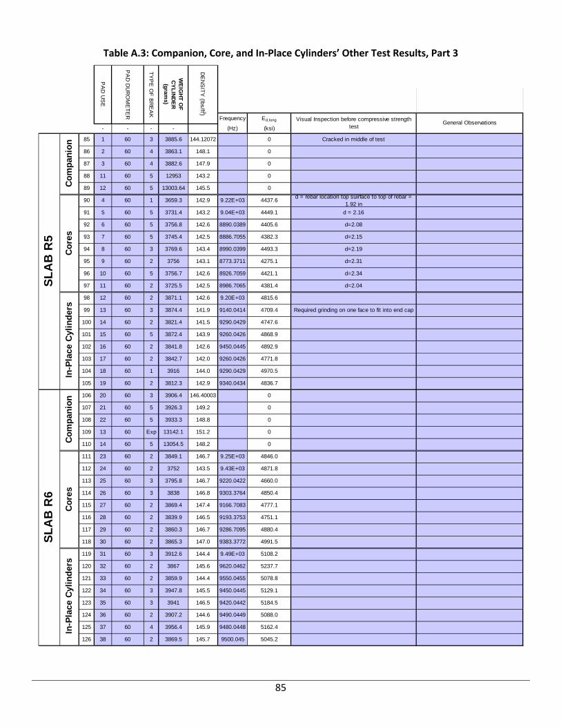
85
Table A.3: Companion, Core, and In‐Place Cylinders’ Other Test Results, Part 3
Frequency Ed,long
- - - - (Hz) (ksi)
85 1 60 3 3885.6 144.12072 0 Cracked in middle of test
86 2 60 4 3863.1 148.1 0
87 3 60 4 3882.6 147.9 0
88 11 60 5 12953 143.2 0
89 12 60 5 13003.64 145.5 0
90 4 60 1 3659.3 142.9 9.22E+03 4437.6d = rebar location top suirface to top of rebar =
1.92 in
91 5 60 5 3731.4 143.2 9.04E+03 4449.1 d = 2.16
92 6 60 5 3756.8 142.6 8890.0389 4405.6 d=2.08
93 7 60 5 3745.4 142.5 8886.7055 4382.3 d=2.15
94 8 60 3 3769.6 143.4 8990.0399 4493.3 d=2.19
95 9 60 2 3756 143.1 8773.3711 4275.1 d=2.31
96 10 60 5 3756.7 142.6 8926.7059 4421.1 d=2.34
97 11 60 2 3725.5 142.5 8986.7065 4381.4 d=2.04
98 12 60 2 3871.1 142.6 9.20E+03 4815.6
99 13 60 3 3874.4 141.9 9140.0414 4709.4 Required grinding on one face to fit into end cap
100 14 60 2 3821.4 141.5 9290.0429 4747.6
101 15 60 5 3872.4 143.9 9260.0426 4868.9
102 16 60 2 3841.8 142.6 9450.0445 4892.9
103 17 60 2 3842.7 142.0 9260.0426 4771.8
104 18 60 1 3916 144.0 9290.0429 4970.5
105 19 60 2 3812.3 142.9 9340.0434 4836.7
106 20 60 3 3906.4 146.40003 0
107 21 60 5 3926.3 149.2 0
108 22 60 5 3933.3 148.8 0
109 13 60 Exp 13142.1 151.2 0
110 14 60 5 13054.5 148.2 0
111 23 60 2 3849.1 146.7 9.25E+03 4846.0
112 24 60 2 3752 143.5 9.43E+03 4871.8
113 25 60 3 3795.8 146.7 9220.0422 4660.0
114 26 60 3 3838 146.8 9303.3764 4850.4
115 27 60 2 3869.4 147.4 9166.7083 4777.1
116 28 60 2 3839.9 146.5 9193.3753 4751.1
117 29 60 2 3860.3 146.7 9286.7095 4880.4
118 30 60 2 3865.3 147.0 9383.3772 4991.5
119 31 60 3 3912.6 144.4 9.49E+03 5108.2
120 32 60 2 3867 145.6 9620.0462 5237.7
121 33 60 2 3859.9 144.4 9550.0455 5078.8
122 34 60 3 3947.8 145.5 9450.0445 5129.1
123 35 60 3 3941 146.5 9420.0442 5184.5
124 36 60 2 3907.2 144.6 9490.0449 5088.0
125 37 60 4 3956.4 145.9 9480.0448 5162.4
126 38 60 2 3869.5 145.7 9500.045 5045.2
TY
PE
OF
BR
EA
K
DE
NS
ITY
(lbs/ft 3)
Visual Inspection before compressive strength test
General Observations
PA
D D
UR
OM
ET
ER
PA
D U
SE
WE
IGH
T O
F
CY
LIN
DE
R
(gram
s)
SL
AB
R5
Co
mp
anio
nC
ore
sIn
-Pla
ce C
ylin
der
s
SL
AB
R6
Co
mp
anio
nC
ore
sIn
-Pla
ce C
ylin
der
s
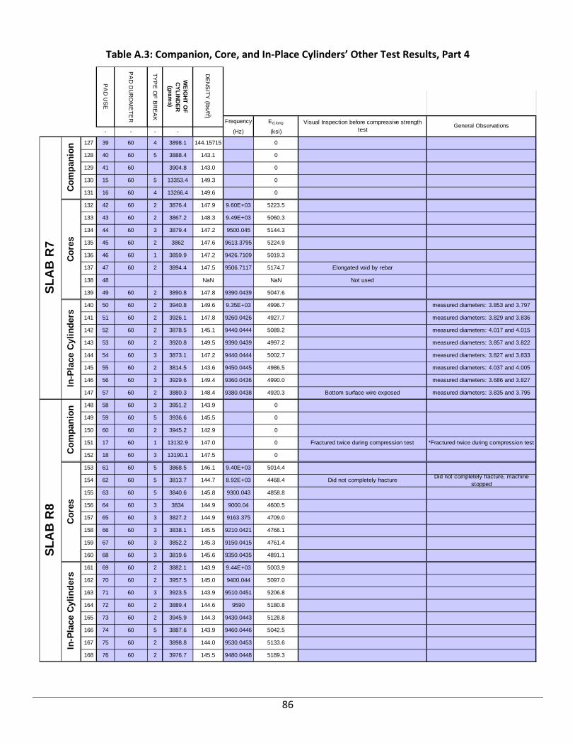
86
Table A.3: Companion, Core, and In‐Place Cylinders’ Other Test Results, Part 4
Frequency Ed,long
- - - - (Hz) (ksi)
127 39 60 4 3898.1 144.15715 0
128 40 60 5 3888.4 143.1 0
129 41 60 3904.8 143.0 0
130 15 60 5 13353.4 149.3 0
131 16 60 4 13266.4 149.6 0
132 42 60 2 3876.4 147.9 9.60E+03 5223.5
133 43 60 2 3867.2 148.3 9.49E+03 5060.3
134 44 60 3 3879.4 147.2 9500.045 5144.3
135 45 60 2 3862 147.6 9613.3795 5224.9
136 46 60 1 3859.9 147.2 9426.7109 5019.3
137 47 60 2 3894.4 147.5 9506.7117 5174.7 Elongated void by rebar
138 48 NaN NaN Not used
139 49 60 2 3890.8 147.8 9390.0439 5047.6
140 50 60 2 3940.8 149.6 9.35E+03 4996.7 measured diameters: 3.853 and 3.797
141 51 60 2 3926.1 147.8 9260.0426 4927.7 measured diameters: 3.829 and 3.836
142 52 60 2 3878.5 145.1 9440.0444 5089.2 measured diameters: 4.017 and 4.015
143 53 60 2 3920.8 149.5 9390.0439 4997.2 measured diameters: 3.857 and 3.822
144 54 60 3 3873.1 147.2 9440.0444 5002.7 measured diameters: 3.827 and 3.833
145 55 60 2 3814.5 143.6 9450.0445 4986.5 measured diameters: 4.037 and 4.005
146 56 60 3 3929.6 149.4 9360.0436 4990.0 measured diameters: 3.686 and 3.827
147 57 60 2 3880.3 148.4 9380.0438 4920.3 Bottom surface wire exposed measured diameters: 3.835 and 3.795
148 58 60 3 3951.2 143.9 0
149 59 60 5 3936.6 145.5 0
150 60 60 2 3945.2 142.9 0
151 17 60 1 13132.9 147.0 0 Fractured twice during compression test *Fractured twice during compression test
152 18 60 3 13190.1 147.5 0
153 61 60 5 3868.5 146.1 9.40E+03 5014.4
154 62 60 5 3813.7 144.7 8.92E+03 4468.4 Did not completely fractureDid not completely fracture, machine
stopped
155 63 60 5 3840.6 145.8 9300.043 4858.8
156 64 60 3 3834 144.9 9000.04 4600.5
157 65 60 3 3827.2 144.9 9163.375 4709.0
158 66 60 3 3838.1 145.5 9210.0421 4766.1
159 67 60 3 3852.2 145.3 9150.0415 4761.4
160 68 60 3 3819.6 145.6 9350.0435 4891.1
161 69 60 2 3882.1 143.9 9.44E+03 5003.9
162 70 60 2 3957.5 145.0 9400.044 5097.0
163 71 60 3 3923.5 143.9 9510.0451 5206.8
164 72 60 2 3889.4 144.6 9590 5180.8
165 73 60 2 3945.9 144.3 9430.0443 5128.8
166 74 60 5 3887.6 143.9 9460.0446 5042.5
167 75 60 2 3898.8 144.0 9530.0453 5133.6
168 76 60 2 3976.7 145.5 9480.0448 5189.3
TY
PE
OF
BR
EA
K
DE
NS
ITY
(lbs/ft 3)
Visual Inspection before compressive strength test
General Observations
PA
D D
UR
OM
ET
ER
PA
D U
SE
WE
IGH
T O
F
CY
LIN
DE
R
(gram
s)
SL
AB
R7
Co
mp
anio
nC
ore
sIn
-Pla
ce C
ylin
der
s
SL
AB
R8
Co
mp
anio
nC
ore
sIn
-Pla
ce C
ylin
der
s

87
Table A.3: Companion, Core, and In‐Place Cylinders’ Other Test Results, Part 5
Frequency Ed,long
- - - - (Hz) (ksi)
169 77 60 1 3875.7 144.8 0 Some companion cylinders with visible porosity
170 78 60 3 3861.1 144.1 0
171 79 60 5 3788.1 141.9 0
172 19 60 5 12760.1 143.6 0
173 20 60 5 12760.7 143.8 0
174 80 60 5 3781.6 142.3 9.38E+03 4859.3
175 81 60 Exp 3797.1 142.5 9.51E+03 4995.6
176 82 60 2 3755.5 142.2 9460.0446 4879.9
177 83 60 3 3737.8 142.9 9600.046 4948.4
178 84 60 4 3781.9 142.6 9380.0438 4853.6
179 85 60 Exp 3773.5 141.7 9380.0438 4832.5
180 86 60 3 3753.6 141.7 9530.0453 4886.6
181 87 60 4 3757.2 143.6 9560.0456 4959.4
182 88 60 4 3899.8 140.5 9.22E+03 4858.2
183 89 60 5 3835.3 140.0 9250.0425 4747.1
184 90 60 2 3847.6 141.3 9300.043 4823.3
185 91 60 5 3837.3 141.8 9250.0425 4808.0
186 92 60 4 3829 140.9 9380.0438 4889.0
187 93 60 2 3851.1 142.3 9230.0423 4820.8
188 94 60 2 3843.6 142.6 9320.0432 4888.4
189 95 60 5 3807.3 141.3 9430.0443 4922.9
190 96 60 4 3940.5 146.5 0
191 97 60 5 3911.8 145.2 0
192 98 60 1 3962.9 146.2 0
193 21 60 Exp 13159.6 145.2 0 Specimen exploded.
194 22 60 5 13183.2 146.7 0
195 1 60 2 3866.1 146.9 9.80E+03 5450.6
196 2 60 Exp 3844.5 146.7 9.77E+03 5371.3
197 3 60 Exp 3799.9 146.1 9850.0485 5345.8Core 2 started the new pads; specimen
exploded
198 4 60 1 3823 145.8 9676.7134 5235.2 At 1.5" a 1/2" void
199 5 60 3 3821.1 146.4 9750.0475 5290.7 At 1.25" a 1/4" void; At 1.9" a 1/2" void
200 6 60 5 3825.1 145.8 9710.0471 5252.9 At 3" a 1.5" void Unplugged Forney power supply
201 7 60 5 3810.1 144.9 9590.0459 5133.7 At 1.1" a 1/2" void; at 2.5" a 1" void
202 8 60 5 3919.5 148.1 9780.0478 5527.4 At 3" a 1" void; at 3.25" a 1" void The side with voids failed quickly
203 9 60 Exp 3977 146.6 9.71E+03 5503.9 At 7" a 1/2" void Specimen exploded.
204 10 60 2 4039.3 146.1 9630.0463 5518.0
205 11 60 3 4027.6 146.5 9700.047 5482.1
206 12 60 3 4001.2 146.7 9690.0469 5528.6 At 7" a 3/4" void Load did not hold
207 13 60 3 4062.7 146.3 9530.0453 5445.2 Oblong deformation from mold
208 14 60 Exp 4062.3 146.7 9580.0458 5517.4 Specimen exploded.
209 15 60 3 3952 145.7 9770.0477 5480.5 At 5.25" a 1/2" void
210 16 60 2 3975 146.0 9680.0468 5475.3
TY
PE
OF
BR
EA
K
DE
NS
ITY
(lbs/ft 3)
Visual Inspection before compressive strength test
General Observations
PA
D D
UR
OM
ET
ER
PA
D U
SE
WE
IGH
T O
F
CY
LIN
DE
R
(gram
s)
SL
AB
R9
Co
mp
anio
nC
ore
sIn
-Pla
ce C
ylin
der
s
SL
AB
R10
Co
mp
anio
nC
ore
sIn
-Pla
ce C
ylin
der
s

88
Table A.3: Companion, Core, and In‐Place Cylinders’ Other Test Results, Part 6
Frequency Ed,long
- - - - (Hz) (ksi)
211 17 60 1 4024.2 145.92079 0
212 18 60 3 3970.7 146.2 0
213 19 60 1 4033.2 145.8 0
214 23 60 5 13114.8 146.4 0
215 24 60 5 13117.6 147.6 0
216 20 60 3 3830.8 144.3 9.54E+03 5122.2
217 21 60 2 3835.7 144.1 9.56E+03 5174.2
218 22 60 2 3842 144.7 9500.045 5110.1
219 23 60 5 3844.7 145.1 9560.0456 5163.7
220 24 60 3 3852.6 145.7 9730.0473 5336.9
221 25 60 2 3810.5 144.5 9630.0463 5150.4
222 26 60 2 3841.1 144.2 9540.0454 5157.0
223 27 60 2 3842.9 144.8 9610.0461 5222.9
224 28 60 5 3911.1 142.3 9.90E+03 5455.8
225 29 60 3 3927.1 146.4 9830.0483 5526.7
226 30 60 Exp 4015.1 147.0 9790.0479 5655.9
227 31 60 2 3955.3 146.2 9710.0471 5476.2
228 32 60 5 3970.4 146.3 9780.0478 5540.6
229 33 60 3 3993.8 146.0 9800.048 5558.7
230 34 60 3 4002.9 147.2 9830.0483 5634.5
231 35 60 2 3994.8 145.2 9690.0469 5448.1
232 39 60 1 3747 141.4487 0
233 40 60 Exp 3756.3 141.8 0
234 41 60 Exp 3746.6 142.1 0
235 27 60 Exp 12905.9 143.4 0
236 28 60 5 12890.2 143.1 0
237 58 60 2 3645.9 138.5 9.20E+03 4493.4
238 59 60 5 3652 138.5 9.23E+03 4547.6 1/2 inch void 2 inches down the top
239 60 60 5 3671.7 138.2 9340.0434 4704.4
240 61 60 3 3663.2 139.1 9293.3763 4615.4
241 62 60 5 3572.6 135.5 9340.0434 4546.0
242 63 60 5 3619.7 137.4 9310.0431 4564.4
243 64 60 5 3632.7 136.6 9263.376 4594.3
244 65 60 5 3656.1 138.6 9240.0424 4538.8
245 66 60 Exp 3696.6 138.8 9.38E+03 4765.8
246 67 60 Exp 3704.2 139.8 9360.0436 4706.3
247 68 60 Exp 3723.7 139.8 9360.0436 4775.3
248 69 60 Exp 3697.5 139.3 9410.0441 4779.7
249 70 60 5 3706 139.8 9390.0439 4756.8
250 71 60 5 3740.2 140.4 9370.0437 4788.8
251 72 60 5 3742 140.4 9453.3779 4872.7
252 73 60 5 3666.1 138.3 9420.0442 4722.2
TY
PE
OF
BR
EA
K
DE
NS
ITY
(lbs/ft 3)
Visual Inspection before compressive strength test
General Observations
PA
D D
UR
OM
ET
ER
PA
D U
SE
WE
IGH
T O
F
CY
LIN
DE
R
(gram
s)
SL
AB
R11
Co
mp
anio
nC
ore
sIn
-Pla
ce C
ylin
der
s
SL
AB
R12
Co
mp
anio
nC
ore
sIn
-Pla
ce C
ylin
der
s
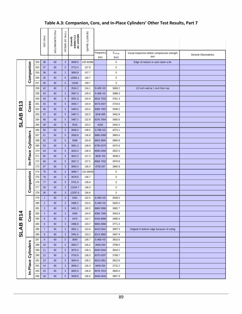
89
Table A.3: Companion, Core, and In‐Place Cylinders’ Other Test Results, Part 7
Frequency Ed,long
- - - - (Hz) (ksi)
253 36 60 3 3658.5 135.92386 0 Edge on bottom is worn down a bit
254 37 60 5 3713.4 137.8 0
255 38 60 2 3693.8 137.7 0
256 25 60 5 12583.1 140.7 0
257 26 60 5 12540 139.7 0
258 42 60 2 3534.2 134.1 8.42E+03 3669.2 1/2 inch void at 1 inch from top
259 43 60 2 3567.4 135.0 8.40E+03 3688.3
260 44 60 5 3551.6 134.9 8516.7018 3761.3
261 45 60 5 3550.7 134.9 8470.0347 3734.6
262 46 60 5 3483.5 133.0 8366.7003 3548.2
263 47 60 5 3487.3 132.0 8236.699 3462.8
264 48 60 5 3487.2 132.8 8376.7004 3560.6
265 49 60 5 3516 133.2 8160 3442.0
266 50 60 5 3648.4 138.5 8.76E+03 4073.1
267 51 60 5 3558.8 136.8 8680.0368 3865.6
268 52 60 5 3568 134.8 8603.3694 3865.8
269 53 60 5 3661.3 138.8 8790.0379 4075.9
270 54 60 5 3633.4 136.9 8590.0359 3922.5
271 55 60 5 3622.2 137.3 8636.703 3938.0
272 56 60 5 3657.2 137.5 8656.7032 3979.8
273 57 60 3 3600.4 136.4 8700.037 3960.8
274 75 60 2 3680.7 132.56628 0
275 76 60 3 3678.6 136.7 0
276 77 60 5 3701.9 135.8 0
277 29 60 3 12234.7 136.9 0
278 30 60 3 12297.6 136.6 0
279 1 60 3 3451 132.0 8.40E+03 3548.5
280 2 60 3 3489.2 133.0 8.44E+03 3630.0
281 3 60 3 3401.3 130.5 8660.0366 3682.7
282 4 60 3 3494 134.0 8396.7006 3563.8
283 5 60 3 3470 132.7 8326.6999 3480.6
284 6 60 3 3486.8 133.7 8660.0366 3771.3
285 7 60 3 3501.1 133.8 8410.0341 3587.5 chipped in bottom edge because of coring
286 8 60 3 3491.6 133.2 8313.3665 3497.9
287 9 60 5 3640 136.7 8.46E+03 3816.6
288 10 60 2 3653.7 136.2 8400.034 3798.6
289 11 60 5 3676.4 136.3 8440.0344 3818.2
290 12 60 2 3703.9 136.0 8370.0337 3768.7
291 13 60 3 3604.9 136.2 8510.0351 3813.9
292 14 60 3 3606.2 135.3 8400.034 3722.2
293 15 60 3 3653.5 136.8 8476.7014 3845.0
294 16 60 5 3639.8 136.6 8440.0344 3807.9
TY
PE
OF
BR
EA
K
DE
NS
ITY
(lbs/ft 3)
Visual Inspection before compressive strength test
General Observations
PA
D D
UR
OM
ET
ER
PA
D U
SE
WE
IGH
T O
F
CY
LIN
DE
R
(gra
ms)
SL
AB
R1
3
Co
mp
an
ion
Co
res
In-P
lace C
yli
nd
ers
SL
AB
R14
Co
mp
an
ion
Co
res
In-P
lace C
yli
nd
ers
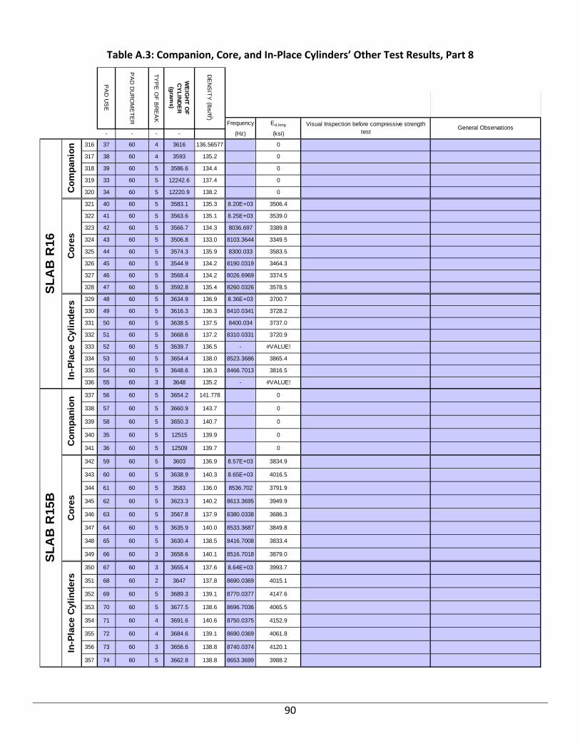
90
Table A.3: Companion, Core, and In‐Place Cylinders’ Other Test Results, Part 8
Frequency Ed,long
- - - - (Hz) (ksi)
316 37 60 4 3616 136.56577 0
317 38 60 4 3593 135.2 0
318 39 60 5 3586.6 134.4 0
319 33 60 5 12242.6 137.4 0
320 34 60 5 12220.9 138.2 0
321 40 60 5 3583.1 135.3 8.20E+03 3506.4
322 41 60 5 3563.6 135.1 8.25E+03 3539.0
323 42 60 5 3566.7 134.3 8036.697 3389.8
324 43 60 5 3506.8 133.0 8103.3644 3349.5
325 44 60 5 3574.3 135.9 8300.033 3583.5
326 45 60 5 3544.9 134.2 8190.0319 3464.3
327 46 60 5 3568.4 134.2 8026.6969 3374.5
328 47 60 5 3592.8 135.4 8260.0326 3578.5
329 48 60 5 3634.9 136.9 8.36E+03 3700.7
330 49 60 5 3616.3 136.3 8410.0341 3728.2
331 50 60 5 3638.5 137.5 8400.034 3737.0
332 51 60 5 3668.6 137.2 8310.0331 3720.9
333 52 60 5 3639.7 136.5 - #VALUE!
334 53 60 5 3654.4 138.0 8523.3686 3865.4
335 54 60 5 3648.6 136.3 8466.7013 3816.5
336 55 60 3 3648 135.2 - #VALUE!
337 56 60 5 3654.2 141.778 0
338 57 60 5 3660.9 143.7 0
339 58 60 5 3650.3 140.7 0
340 35 60 5 12515 139.9 0
341 36 60 5 12509 139.7 0
342 59 60 5 3603 136.9 8.57E+03 3834.9
343 60 60 5 3638.9 140.3 8.65E+03 4016.5
344 61 60 5 3583 136.0 8536.702 3791.9
345 62 60 5 3623.3 140.2 8613.3695 3949.9
346 63 60 5 3567.8 137.9 8380.0338 3686.3
347 64 60 5 3635.9 140.0 8533.3687 3849.8
348 65 60 5 3630.4 138.5 8416.7008 3833.4
349 66 60 3 3658.6 140.1 8516.7018 3879.0
350 67 60 3 3655.4 137.6 8.64E+03 3993.7
351 68 60 2 3647 137.8 8690.0369 4015.1
352 69 60 5 3689.3 139.1 8770.0377 4147.6
353 70 60 5 3677.5 138.6 8696.7036 4065.5
354 71 60 4 3691.6 140.6 8750.0375 4152.9
355 72 60 4 3684.6 139.1 8690.0369 4061.8
356 73 60 3 3656.6 138.8 8740.0374 4120.1
357 74 60 5 3662.8 138.8 8653.3699 3988.2
TY
PE
OF
BR
EA
K
DE
NS
ITY
(lbs/ft 3)
Visual Inspection before compressive strength test
General Observations
PA
D D
UR
OM
ET
ER
PA
D U
SE
WE
IGH
T O
F
CY
LIN
DE
R
(gram
s)
SL
AB
R1
6
Co
mp
anio
nC
ore
sIn
-Pla
ce C
yli
nd
ers
SL
AB
R15
B
Co
mp
an
ion
Co
res
In-P
lace
Cyl
ind
ers
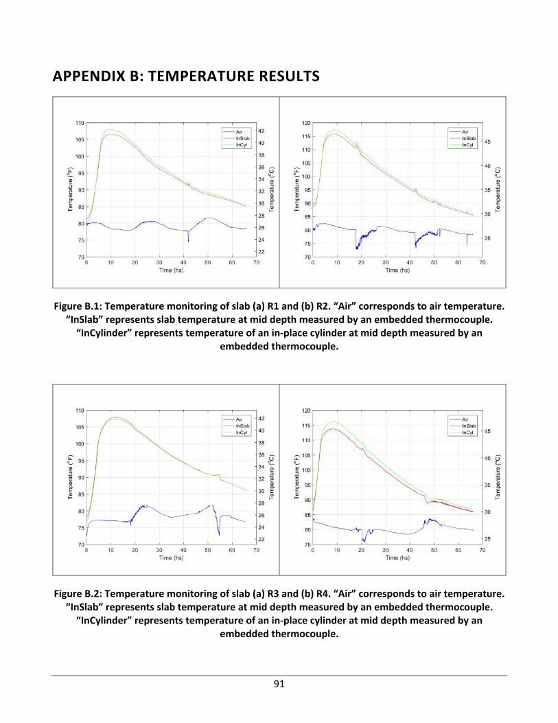
91
APPENDIX B: TEMPERATURE RESULTS
Figure B.1: Temperature monitoring of slab (a) R1 and (b) R2. “Air” corresponds to air temperature. “InSlab” represents slab temperature at mid depth measured by an embedded thermocouple. “InCylinder” represents temperature of an in‐place cylinder at mid depth measured by an
embedded thermocouple.
Figure B.2: Temperature monitoring of slab (a) R3 and (b) R4. “Air” corresponds to air temperature. “InSlab” represents slab temperature at mid depth measured by an embedded thermocouple. “InCylinder” represents temperature of an in‐place cylinder at mid depth measured by an
embedded thermocouple.
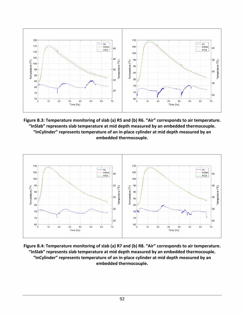
92
Figure B.3: Temperature monitoring of slab (a) R5 and (b) R6. “Air” corresponds to air temperature. “InSlab” represents slab temperature at mid depth measured by an embedded thermocouple. “InCylinder” represents temperature of an in‐place cylinder at mid depth measured by an
embedded thermocouple.
Figure B.4: Temperature monitoring of slab (a) R7 and (b) R8. “Air” corresponds to air temperature. “InSlab” represents slab temperature at mid depth measured by an embedded thermocouple. “InCylinder” represents temperature of an in‐place cylinder at mid depth measured by an
embedded thermocouple.

93
Figure B.5: Temperature monitoring of slab (a) R9 and (b) R10. “Air” corresponds to air temperature. “InSlab” represents slab temperature at mid depth measured by an embedded
thermocouple. “InCylinder” represents temperature of an in‐place cylinder at mid depth measured by an embedded thermocouple.
Figure B.6: Temperature monitoring of slab (a) R11 and (b) R12. “Air” corresponds to air temperature. “InSlab” represents slab temperature at mid depth measured by an embedded
thermocouple. “InCylinder” represents temperature of an in‐place cylinder at mid depth measured by an embedded thermocouple.
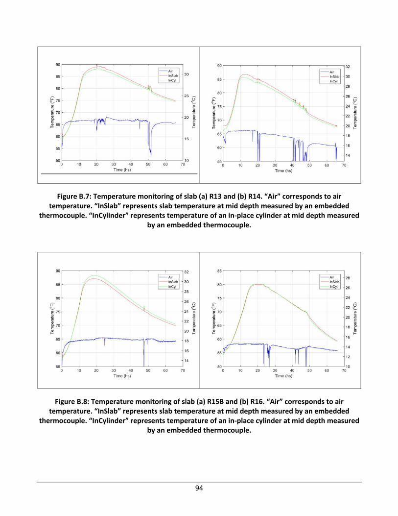
94
Figure B.7: Temperature monitoring of slab (a) R13 and (b) R14. “Air” corresponds to air temperature. “InSlab” represents slab temperature at mid depth measured by an embedded
thermocouple. “InCylinder” represents temperature of an in‐place cylinder at mid depth measured by an embedded thermocouple.
Figure B.8: Temperature monitoring of slab (a) R15B and (b) R16. “Air” corresponds to air temperature. “InSlab” represents slab temperature at mid depth measured by an embedded
thermocouple. “InCylinder” represents temperature of an in‐place cylinder at mid depth measured by an embedded thermocouple.

95
APPENDIX C: DENSITY STUDY FOR CONSOLIDATION PROCEDURE ASSESSEMENT
C.1 INTRODUCTION
IDOT’s research project “Evaluation of PCC Pavement and Structure Coring and In Situ Testing Alternatives” consists of comparing the strength of cores to in‐place cylinders at a certain age in order to identify the inherent damage that coring does to concrete. For this purpose, both kinds of cylinders should have equal or very similar compaction so as to produce equally dense concrete. The objective of this set of experiments was to identify the best vibrating method among several options to ensure similar consolidation between cores and in‐place cylinders.
C.2 APPROACH C.2.1 General
Four compacting methods were tested:
Rodding
Internal vibration
Plastic‐mold (external) vibration
Sleeve (external) vibration
Two slabs were cast, Slab 5 (S5) and Slab 6 (S6). Slab 5 produced eight cores, eight in‐place cylinders, and three companion cylinders. Slab 6 produced seven cores, eight in‐place cylinders, and three companion cylinders. Companion cylinders are not analyzed in this report. All cores were sawed at the bottom to obtain 4 x 8 in. (10 x 20 cm) cylinders.
Within Slab 5, four of its in‐place cylinders were rodded and the rest internally vibrated. Within Slab 6, four of its cylinders were consolidated with the plastic‐mold vibration method and the rest with the sleeve vibration method.
Both slabs were cured for 3 days. Cores and in‐place cylinders were extracted on the 7th day after casting. After that, they were submerged in water at 73°F (23°C) for 24 hours to achieve saturation. Mass and volume measurements were then taken to calculate density. These measurements were done on the 8th day after casting (Trial 1), and another set of measurements was taken the 14th day after casting (Trial 2). During both trials, all cylinders were maintained submerged in water at 73°F (23°C). All of the following measurements, results, and conclusions refer to Trial 2.
In summary, four different groups of in‐place cylinders were tested by comparing their densities to the densities of their corresponding cores.
96
C.2.2 Density Methods
Two different methods were followed to calculate density.
The first method (geometric) consisted of calculating the volume of the samples by measuring diameter (average of three measurements) and height (average of two measurements), as established in ASTM C39 and AASHTO T22, to obtain an average sample’s volume. The mass of each sample was then obtained by weighing the samples in a saturated surface dry (SSD) condition, and densities were calculated by simple division of weight over volume. Diameter was measured by using a clamp‐like tool to set the sample diameter at the mid height, and then using a caliper. Height was measured with metric tape.
The second method (submerged method) consisted of calculating the volume samples by weighing the samples submerged, as established in ASTM C39 and AASHTO T22. Thus, the following formula was used to compute the samples’ volumes:
(C1)
where W is the air weight of the sample, Ws is the submerged weight, and γs is the water density. Density was calculated by simple division between W over V.
C.2.3 Rodding Compaction Details
Rodding compaction was done following ASTM C39 and AASHTO T22. All four rodded cylinders were cast and finished outside the formwork and then put inside the form and fixed to the metal bracers. There, each cylinder was filled in two layers. Each layer was rodded 25 times and tapped 10 times. Finishing was done with metal trowel.
C.2.4 Internal Vibration Details
This procedure was done by following the specifications in ASTM C31 and AASHTO T23. Internal vibration was performed with the plastic molds already in position held by the metal bracers. Each cylinder was filled in two layers. Each layer was vibrated by introducing the vibrator into the concrete and holding it for 4 to 5 seconds before slowly removing it. All cylinders´ sleeves were tapped with a rubber mallet 10 times after filling each layer. Finishing was done with metal trowel.
C.2.5 Plastic Mold (External) Vibration
Only one brief reference to external vibration was found in ASTM standards document ASTM C873, which says to “use the vibrator externally, briefly touching the exterior of the mold support member.” All four plastic‐mold vibrated cylinders were cast and finished outside the formwork and then put inside the formwork fixed to the metal bracers. They were filled in two layers. Each layer was compacted by touching the plastic mold at four equally distributed points of the plastic mold (outer surface of the mold at approximately mid height of the layer), for 4 to 5 seconds per touch. After the four touches were done, each mold was tapped 10 times (each layer).

97
C.2.6 Sleeve (External) Vibration
Sleeve vibration was performed with the plastic molds already in position held by the metal bracers. Each cylinder was filled in two layers. Each layer was externally vibrated by touching the outer sleeve in three locations equally distributed for 4 to 5 seconds (three rather than four locations were chosen in order to avoid over‐vibrating the rest of the slab). In this case, half the slab´s height was filled with concrete, then the first layer of the cylinders was filled and compacted, then the rest of the slab was filled with concrete. Finally, the second layer of the cylinders was filled, vibrated, and finished (see the procedure for Slab 6 below). These cylinders were not tapped.
C.2.7 Vibration of Slab Concrete
The concrete was vibrated using the internal vibrator following recommended practice: the vibrating head was inserted vertically downward into the concrete at a rapid rate but without touching the bottom of the form, and then it was more slowly lifted vertically to the surface (Mindess et al. 2003). The vibrator used generated 14,000 rpm. Thus, its radius of action was estimated to be around 4 in. (10 cm). For 4 in. (10 cm) slump concrete with 6.5% entrained air, the estimated insertion time is 4 to 5 seconds. The vibrator was therefore inserted vertically, at a regular spacing, at 4 to 5 seconds. The insertion spacing was around 6 in. (15 cm), which is 1.5 times the radius of action (Mindess et al. 2003).
C3 PROCEDURE
C.3.1 Slab 5—Rodding and Internal Vibration
Concrete specifications were checked (slump, air content, and mix design).
Four cylinders were placed outside the formwork and filled following the rodding method (filled in two layers, rodded 25 times, tapped 10 times, finished, and placed in final position).
The remaining four cylinders were filled following the internal vibration method (filled in two layers, vibrator introduced, tapped 10 times, and finished).
The rest of the slab was filled with concrete, vibrated, and finished.
C.3.2 Slab 6—Plastic‐Mold (External) Vibration and Sleeve (External) Vibration
Concrete specifications were checked (slump, air content, and mix design).
Four cylinders were placed outside the formwork and filled following the plastic‐mold vibration method (filled in two layers, externally vibrated by touching the plastic mold at four locations for 5 seconds each, tapped 10 times, finished, and placed in final position).
Half of the slab was filled.
The remaining four cylinders were filled to half their height, and the sleeve vibration method was performed.
The second half of the slab was poured.
The second layer of the sleeve‐vibrated cylinders was filled and vibrated.
The rest of the slab was vibrated and finished.

98
C.4 RESULTS
Visual inspection was performed to account for external defects. It was found that two of the rodded cylinders presented poor compaction at the bottom edge. In addition, one of the internally vibrated cylinders presented several superficial air voids, with dimensions of 0.75 in. (2 cm) deep and 0.5 in. (1 cm) diameter; two other internally vibrated cylinders also presented visible voids of the order of 0.5 in. (1 cm) deep and 0.5 in. (1 cm) diameter in several locations.
The Table C.1 presents the density results of the second set of experiments (Trial 2).
Table C.1: Density Results*
TRIAL 2
Geometric Volume Method Submerged Volume Method
Average Density (lb/ft3)
Relative Difference to Cores
(%)
Standard Deviation (lb/ft3)
CV (std/ave)
(%)
Average Density (lb/ft3)
Relative Difference to Cores
(%)
Standard Deviation (lb/ft3)
CV (std/ave)
(%)
Rodded 145.2 0.2 1.0 0.7 145.1 0.2 0.4 0.3
Internally Vibrated 146.1 0.7 0.9 0.6 145.2 0.3 0.3 0.2
Cores_S5 145.0 — 0.6 0.4 144.7 — 0.3 0.2
Plastic Mold 147.9 0.6 1.7 1.1 145.2 0.5 0.3 0.2
Sleeve 147.7 0.5 0.6 0.4 145.1 0.4 0.3 0.2
Cores_S6 147.1 — 0.8 0.5 144.5 — 0.2 0.2
* 1 lb/ft3 =17.36 kg/m3
Note: The number of samples tested of each cylinder group were four rodded samples, four internally vibrated samples, eight slab 5 cores (Cores_S5), four plastic‐mold vibrated samples, four sleeve‐vibrated samples, and seven slab 6 cores (Core_S6).
In Table C.1, average density corresponds to the average density of each group of cylinders, and relative difference to cores corresponds to the relative difference with respect the corresponding cores of the same slab (i.e., rodded and internally vibrated in‐place cylinders are compared to Cores_S5, whereas plastic‐mold vibrated and sleeve vibrated cylinders are compared to Cores_S6), calculated with the following equation.
. (C2)
Standard deviation corresponds to the standard deviation of each group of cylinders, and CV refers to the coefficient of variation calculated as follows:
% 100 (C3)
C.5 SAW‐CUTTING AND VISUAL INSPECTION
One cylinder from each group was sawed longitudinally to account for potential segregation. The following figures show these results.

99
Figure C.1a: Core 5 (Slab 5) sawed
Figure C.1b: Rodded cylinder 2 sawed
Figure C.1c: Internally vibrated cylinder 3 sawed
Figure C.1b: Core 1 (Slab 6) sawed
Figure C.1d: Plastic‐mold vibrated cylinder 5 sawed
Figure C.1e: Sleeve vibrated cylinder 1 sawed

100
Figure C.1c shows the internally vibrated cylinder. It can be seen in that figure that the insertion of the vibrator generated segregation: the center of the cylinder did not have coarse aggregate, whereas the outer part of the cylinder had much more.
The other figures do not show clear segregation. Only the sleeve‐vibrated cylinder, shown in Figure C.1e, had a 1 in. (2.5 cm) long by 0.1 in. (0.2 cm) wide void/crack. In addition, the transverse middle of that cylinder had a smaller amount of coarse aggregate than did the top and bottom edges.
C.6 ANALYSIS
It should be noted that the submerged volume method is more accurate than the geometric volume method because the former accounts for all superficial anomalies, such as external air voids, open pores, lack of perpendicularity and smoothness at the edges, and variation of diameter along the samples’ height. On the other hand, the latter method assumes the cylinders to be perfectly cylindrical and computes the volume from the average of three heights and the average of three diameter measurements at mid height of the sample.
In looking at the submerged volume method section of Table C.1, it can be seen that all standard deviations were very small, yielding coefficients of variation of less than 0.5% in all cases. In addition, the relative difference of rodded and internally vibrated cylinders compared to Cores_S5 was less than 1%; the same relation was observed when comparing relative differences of plastic‐mold and sleeve cylinders with respect to Cores_S6.
With the geometric volume method, it can be seen in Table C.1 that although the standard deviations increased a little, the coefficients of variation remained less than or around 1%. Furthermore, the corresponding relative differences of in‐place cylinders to cores were also below 1%.
Figures C.2 and C.3 show the average densities of all cylinder groups measured with both methods.

101
Figure C.2: Densities of Slab 5, Trial 2 (1 lb/ft3 = 17.36 kg/m3).
Figure C.3: Densities of Slab 6, Trial 2 (1 lb/ft3 = 17.36 kg/m3).
It can be seen in Figures C.2 and C.3 that the error bars were notably small compared to the density values. It can also be seen that densities calculated with the geometric method were larger than the corresponding ones calculated with the submerged method. Table C.2 provides a quantitative analysis of that observation.
0.0
20.0
40.0
60.0
80.0
100.0
120.0
140.0
160.0
Rodded Internally Cores_S5
Density (lbs/ft3)
Slab 5 Densities ‐ Trial 2
"Geometric"
"Submerged"
0.0
20.0
40.0
60.0
80.0
100.0
120.0
140.0
160.0
Plastic‐Mold Sleeve Cores_S6
Density (lbs/ft3)
Slab 6 Densities ‐ Trial 2
"Geometric"
"Submerged"

102
Table C.2: Density Averages and Errors (1 ls/ft3 = 17.36 kg/m3)
Geometric Volumetric
Method (kg/m3)
Submerged Volumetric
Method (kg/m3) Relative Error to Submerged (%)
Rodded 145.2 145.1 0.1
Internal 146.1 145.2 0.6
Cores_S5 145.0 144.7 0.2
Plastic Mold 147.9 145.2 1.9
Sleeve 147.7 145.1 1.8
Cores_S6 147.1 144.5 1.8
where relative error to submerged is the relative error of the geometric method density with respect to the submerged method density, computed as follows:
. (C4).
It can be seen in Table C.2 that all relative differences are positive—that is, the geometric densities were always higher than the submerged densities. This trend was clearer for Slab 6, with values almost reaching 2%, whereas Slab 5 values were below 0.6% of relative difference. However, in both cases (Slab 5 and Slab 6), the relative difference of the geometric method densities with respect to the submerged method densities was significantly low (below 2% for all cases), which means that the geometric method is sufficiently accurate for this research project because density is not the most important concrete parameter.
However, the systematic density differences between the two methods were opposite the expected trend. The submerged method accounts for the open pores and small external air voids present in concrete; thus, the volume computed by the submerged method tends to be lower than the volume computed by the geometric method. Therefore, the former method tends to yield higher densities than the latter. The results are opposite because of the way volume is measured in the geometric method.
It was explained previously that in the geometric method the diameter was determined by using with a clamp‐like tool and measuring the distance of the clamp with a caliper. It was seen that the clamp makes very small notches around 0.04 in. (1 mm) deep at the concrete surface when diameter is being measured. Thus, the diameter obtained tends to be around 0.08 in. (2 mm) smaller than the actual diameter. This systematic experimental error ends up yielding a theoretical difference of up to 4% between the geometric method and submerged method for calculating density.
C.7 CONCLUSIONS
Four consolidating methods were analyzed to identify the best way to compact slab concrete and in‐place cylinders as similarly as possible. The analysis was done by comparing the cylinders’ densities
103
using two methods: geometric and submerged. The cylinders comprised six groups, categorized by their nature (core or in‐place cylinder) and compacting method (rodded, internally vibrated, plastic mold, sleeve).
When densities were compared by using the submerged method, all four compacting methods showed small relative differences between in‐place cylinders and cores densities (less than 0.5%). In addition, all standard deviations for the six groups of cylinders were very small, yielding coefficients of variation less than or equal to 0.3%.
It was also observed that the experimental procedure conducted to measure volume with the geometric method yielded a systematic error that may go up to 4% of the actual density of each sample. The source of this error lay in the tools being used, and it will be changed in further experiments. In addition, the geometric method tended to yield more variable measurements because it did not account for open pores and external voids—nor did it account for variations in diameter and heights throughout the sample. Nevertheless, the geometric method was able to be performed much faster than the submerged method. Therefore, in the future, if measurements are taken with care and using proper tools, the geometric method could yield accurate results.
Visual inspection was done to each cylinder. It was observed that the rodded cylinders tended to be more porous and had fine honey‐combing at their bottom edges. Internally vibrated cylinders showed large external air voids at their sides. Cores, plastic‐mold vibrated cylinders, and sleeve‐vibrated cylinders did not have significant external defects.
One sample cylinder per group was longitudinally sawed and visual inspection performed on the cut surface. It was found that the internally vibrated cylinder had segregation caused by insertion of the vibrator, which pushed the coarse aggregate far from the center and to the lateral surface of the cylinder. The sleeve‐vibrated cylinder had a small elongated void and a zone with less aggregate in the middle cross‐section; this light segregation could have been caused by the cylinders having been filled in two layers and not being tapped after each layer was vibrated.
Furthermore, it should be noted that the two slabs were vibrated following a systematic pattern of location and time of vibration. This pattern had not been followed with the previous slabs cast for this research project. This fact could have also contributed to the small standard deviations and small relative differences between cylinders and cores. This technique will be maintained for casting further slabs.
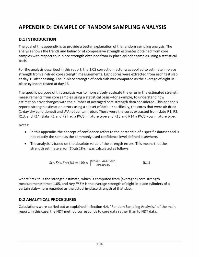
104
APPENDIX D: EXAMPLE OF RANDOM SAMPLING ANALYSIS
D.1 INTRODUCTION
The goal of this appendix is to provide a better explanation of the random sampling analysis. The analysis shows the trends and behavior of compressive strength estimates obtained from core samples with respect to in‐place strength obtained from in‐place cylinder samples using a statistical basis.
For the analysis described in this report, the 1.05 correction factor was applied to estimate in‐place strength from air‐dried core strength measurements. Eight cores were extracted from each test slab at day 15 after casting. The in‐place strength of each slab was computed as the average of eight in‐place cylinders tested at day 16.
The specific purpose of this analysis was to more closely evaluate the error in the estimated strength measurements from core samples using a statistical basis—for example, to understand how estimation error changes with the number of averaged core strength data considered. This appendix reports strength estimation errors using a subset of data—specifically, the cores that were air dried (1‐day dry conditioned) and did not contain rebar. Those were the cores extracted from slabs R1, R2, R13, and R14. Slabs R1 and R2 had a PV/SI mixture type and R13 and R14 a PV/SI‐low mixture type.
Notes:
In this appendix, the concept of confidence refers to the percentile of a specific dataset and is not exactly the same as the commonly used confidence level defined elsewhere.
The analysis is based on the absolute value of the strength errors. This means that the strength estimate error (Str.Est.Err.) was calculated as follows:
. . % 100 . . . . .
. . . (D.1)
where Str.Est. is the strength estimate, which is computed from (averaged) core strength measurements times 1.05, and Avg.IP.Str is the average strength of eight in‐place cylinders of a certain slab—here regarded as the actual in‐place strength of that slab.
D.2 ANALYTICAL PROCEDURES
Calculations were carried out as explained in Section 4.4, “Random Sampling Analysis,” of the main report. In this case, the NDT method corresponds to core data rather than to NDT data.

105
D.3 RESULTS FROM CORE SAMPLES WITHOUT REBAR
Figure D.1 presents the expected strength error curves that show how the expected error of the strength prediction varies with an increasing number of tested cores at three confidence levels (75%, 85%, and 95%).
Figure D.1: Expected strength error curves using correction factor 1.05 for air‐dried cores with no rebar from PV/SI and PV/SI mixtures (data from slabs R1, R2, R13, and R14).
The x‐axis corresponds to the number of tested cores that are used to obtain a single strength measurement. This means that, for a given concrete element cast from a single batch (in this case, emulated with one specific slab), data from either one, two, three, or more cores are considered and averaged to obtain one single core strength value. The 1.05 correction factor is applied to the value to yield the strength estimate of the in‐place concrete.
First consider only the black curve in Figure D.1. That line corresponds to the 95% confidence level, meaning that the y‐axis corresponds to the 95th percentile expected strength error of the estimation in absolute value. Considering that the black line at x = 1 gives y ≈ 7% (meaning that if we were to estimate the in‐place strength by using a single core and multiplying its strength by 1.05), there is a 95% chance that the strength estimation will have an error of 7% or lower with respect to the actual in‐place strength of the selected slab.
If we now we consider the average of two random cores (see x = 2 in Figure D.1, which corresponds to y ≈ 5%), there is a ~95% chance that the calculated strength estimation would have a 5% error or

106
lower with respect to the actual in‐place strength of the slab. A 95% confidence level is usually required for critical infrastructure (nuclear power plants, hospitals, etc.), but for other structures, such as pavements, lower confidence levels of 75% or 85% would be acceptable. At the 75% confidence level (red line), one random core results in an error of 5% or lower, and the average of three cores provides an error of 2.5% or lower—that is, we expect a 25% chance of having an error higher than 2.5%.
Clearly, the error of the strength estimation drops as more cores are extracted and averaged, assuming we maintain the same confidence level of the results. However, it should be noted that in these computations the concrete batches were clearly identified because each batch corresponds to one single slab. Therefore, when computing the strength average from different cores, only cores within the same batch were considered. In actual field application, this may not be so clear, and different cores could be drawn from different concrete batches, which would not represent the in‐place strength of a specific concrete batch. To use these results as guidelines for other applications, strength estimates should come from cores drawn from a single concrete batch. Selection of the required confidence level of the strength estimations should be done by taking into consideration the consequences that may occur if the error in the prediction is higher than the tolerance. As previously noted, for pavements, a 75% to 85% confidence is usually acceptable.
Now consider a different approach to understand the effect of expected error of strength estimations. Figure D.2 presents the histograms created from all the strength estimation errors computed by considering every possible combination of averaged core strength values. These were computed using the same datasets and procedure as explained above. The data in Figure D.1 can be directly obtained by looking at the data shown in Figure D.2.
To understand Figure D.2, first look at the top left subfigure identified as ind = 1. This subfigure represents all the possible strength estimate errors, in absolute value, that are obtained from the experimental dataset. ind = 1 means that only one individual core strength value was used, then the 1.05 factor was applied to that one core to obtain the strength estimate. The percent errors of that estimate with regard to the real in‐place strength value of the slab are shown. The other subfigures (ind = 2, ind = 3, etc.) correspond to the computed strength errors when all possible combinations of two, three, or more core strengths are averaged to obtain the strength estimation.
Note that a total of 32 cores were used in this analysis, corresponding to four different slabs with eight cores per slab. In subfigure ind = 1, N = 32 because there are 32 possible values of core strengths when only one core is used. In subfigure ind = 2, N = 112 because there are 112 possible combinations of cores (in all possible combinations of two) from which to take the average and obtain the strength estimate. This means that if we were to randomly select the strength values of two cores, there are 112 possibilities—thus, there are 112 possible estimated strength errors.

107
Figure D.2: Histograms of percent error of strength estimations in absolute value using a correction factor of 1.05 considering air‐dried cores with no rebar and from PV/SI and PV/SI mixtures only (slabs R1, R2, R13 and R14). “ind” corresponds
to the number of averaged core strength values to obtain the strength estimate and “N” is the total size of the dataset. The vertical red line defines the 5% strength error.
Figure D.2 shows the following:
When strength was estimated using only one core, seven out of 32 possible strength estimates yielded an error higher than 5% (in absolute value); i.e., there is about a 78% chance of obtaining a 5% error or lower.
When strength was estimated using the average of two cores, five out of 112 possible strength estimates yielded an error higher than 5% (in absolute value); i.e., there is about a 96% chance of obtaining 5% error or lower.
When strength was estimated using the average of three cores, one out of 224 possible strength estimates yielded an error higher than 5% (in absolute value); i.e., there is a 99.6% chance of obtaining a 5% error or lower.
When strength was estimated using the average of four or more cores, no estimated strength yielded an error higher than 5%.
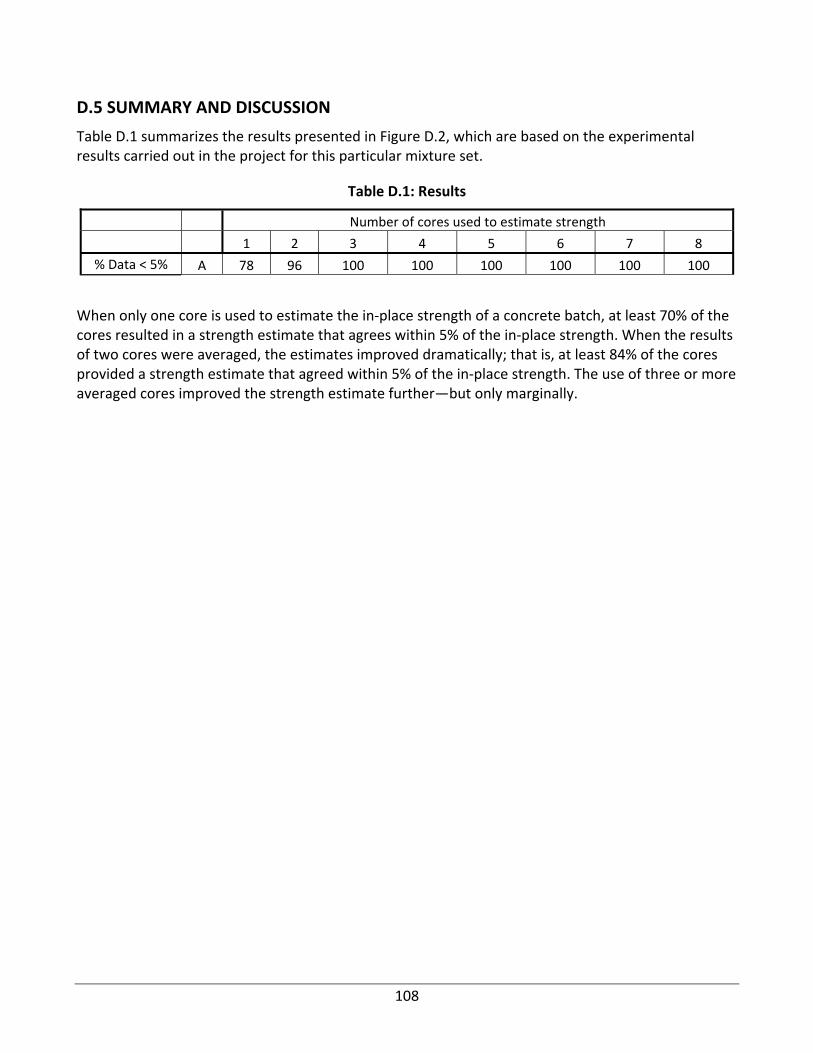
108
D.5 SUMMARY AND DISCUSSION
Table D.1 summarizes the results presented in Figure D.2, which are based on the experimental results carried out in the project for this particular mixture set.
Table D.1: Results
Number of cores used to estimate strength
1 2 3 4 5 6 7 8
% Data < 5% A 78 96 100 100 100 100 100 100
When only one core is used to estimate the in‐place strength of a concrete batch, at least 70% of the cores resulted in a strength estimate that agrees within 5% of the in‐place strength. When the results of two cores were averaged, the estimates improved dramatically; that is, at least 84% of the cores provided a strength estimate that agreed within 5% of the in‐place strength. The use of three or more averaged cores improved the strength estimate further—but only marginally.
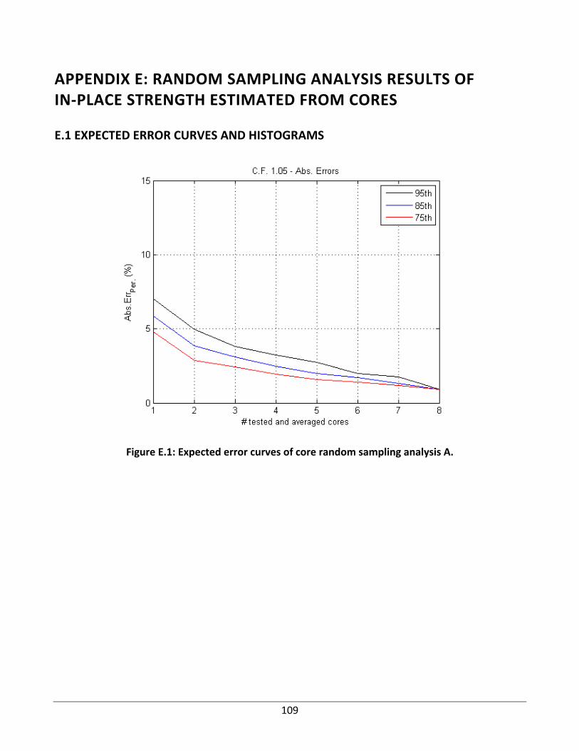
109
APPENDIX E: RANDOM SAMPLING ANALYSIS RESULTS OF IN‐PLACE STRENGTH ESTIMATED FROM CORES
E.1 EXPECTED ERROR CURVES AND HISTOGRAMS
Figure E.1: Expected error curves of core random sampling analysis A.

110
Figure E.2: Dataset histograms of core random sampling analysis A. The red line indicates the 5% error level. Text indicates the number of strength estimates having an error greater than 5%.
Figure E.3: Expected error curves of core random sampling analysis B.

111
Figure E.4: Dataset histograms of core random sampling analysis B. The red line indicates the 5% error level. Text indicates the number of strength estimates having an error greater than 5%.
Figure E.5: Expected error curves of core random sampling analysis C.
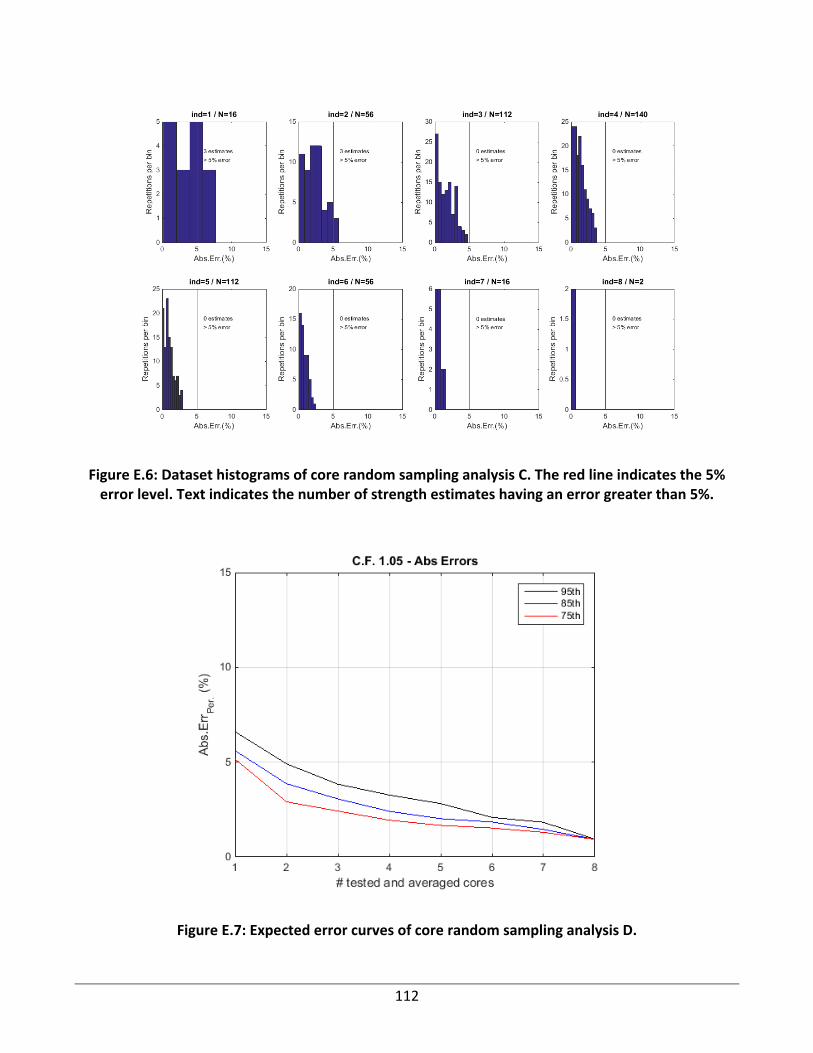
112
Figure E.6: Dataset histograms of core random sampling analysis C. The red line indicates the 5% error level. Text indicates the number of strength estimates having an error greater than 5%.
Figure E.7: Expected error curves of core random sampling analysis D.
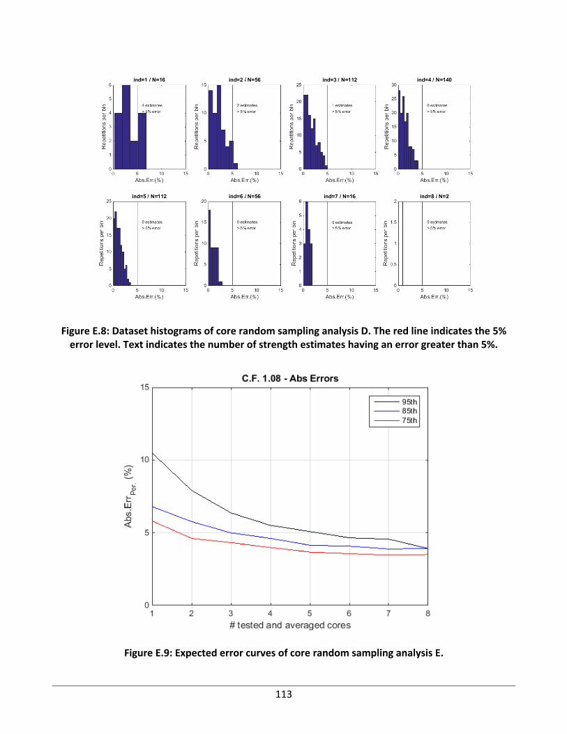
113
Figure E.8: Dataset histograms of core random sampling analysis D. The red line indicates the 5% error level. Text indicates the number of strength estimates having an error greater than 5%.
Figure E.9: Expected error curves of core random sampling analysis E.

114
Figure E.10: Dataset histograms of core random sampling analysis E. The red line indicates the 5% error level. Text indicates the number of strength estimates having an error greater than 5%.
Figure E.11: Expected error curves of core random sampling analysis F.

115
Figure E.12: Dataset histograms of core random sampling analysis F. The red line indicates the 5% error level. Text indicates the number of strength estimates having an error greater than 5%.
Figure E.13: Expected error curves of core random sampling analysis G.
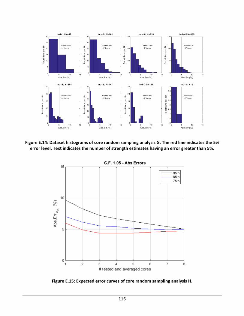
116
Figure E.14: Dataset histograms of core random sampling analysis G. The red line indicates the 5% error level. Text indicates the number of strength estimates having an error greater than 5%.
Figure E.15: Expected error curves of core random sampling analysis H.
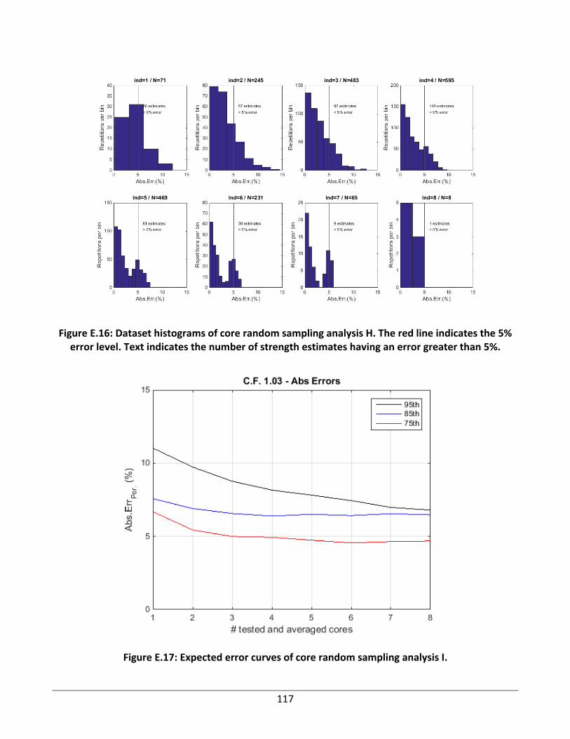
117
Figure E.16: Dataset histograms of core random sampling analysis H. The red line indicates the 5% error level. Text indicates the number of strength estimates having an error greater than 5%.
Figure E.17: Expected error curves of core random sampling analysis I.

118
Figure E.18: Dataset histograms of core random sampling analysis I. The red line indicates the 5% error level. Text indicates the number of strength estimates having an error greater than 5%.
Figure E.19: Expected error curves of core random sampling analysis J.

119
Figure E.20: Dataset histograms of core random sampling analysis J. The red line indicates the 5% error level. Text indicates the number of strength estimates having an error greater than 5%.

120
APPENDIX F: AGGREGATE GRADATIONS
F.1 COARSE AGGREGATE 1, CM16, KANKAKEE
Figure F.1: CM16 aggregate gradation expressed in terms of percentage of aggregate passing through the specified sieve. Provided by Prairie Materials.
F.2 COARSE AGGREGATE 2, CM11, KANKAKEE
Figure F.2: CM11 aggregate gradation expressed in terms of percentage of aggregate passing through the specified sieve. Provided by Prairie Materials.
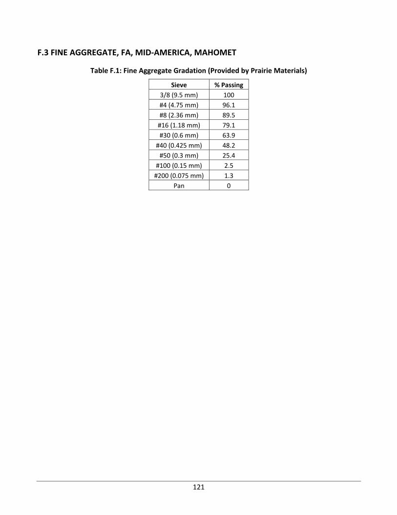
121
F.3 FINE AGGREGATE, FA, MID‐AMERICA, MAHOMET
Table F.1: Fine Aggregate Gradation (Provided by Prairie Materials)
Sieve % Passing
3/8 (9.5 mm) 100
#4 (4.75 mm) 96.1
#8 (2.36 mm) 89.5
#16 (1.18 mm) 79.1
#30 (0.6 mm) 63.9
#40 (0.425 mm) 48.2
#50 (0.3 mm) 25.4
#100 (0.15 mm) 2.5
#200 (0.075 mm) 1.3
Pan 0