Evaluation of empirical approaches to estimate the ... · Evaluation of empirical approaches to...
163
Evaluation of empirical approaches to estimate the variability of erosive inputs in river catchments Dissertation zur Erlangung des akademischen Grades Dr. rer. nat. im Fach Geographie eingereicht an der Mathematisch-Naturwissenschaftlichen Fakultät II der Humboldt-Universität zu Berlin von Diplom-Geoökologe Andreas Gericke Präsident der Humboldt-Universität zu Berlin Prof. Dr. Jan-Hendrik Olbertz Dekan der Mathematisch-Naturwissenschaftlichen Fakultät II Prof. Dr. Elmar Kulke Gutachter 1. Prof. Dr. Gunnar Nützmann, Humboldt-Universität zu Berlin 2. Prof. Dr. Matthias Zessner, Technische Universität Wien 3. PD Dr. Jürgen Hofmann, Leibniz-Institut für Gewässerökologie und Binnenfischerei Tag der Verteidigung: 16.10.2013
Transcript of Evaluation of empirical approaches to estimate the ... · Evaluation of empirical approaches to...

Evaluation of empirical approaches to estimate the variability of erosive
inputs in river catchments
Dissertation zur Erlangung des akademischen Grades Dr. rer. nat.
im Fach Geographie
eingereicht an der Mathematisch-Naturwissenschaftlichen Fakultät II der Humboldt-Universität zu Berlin
von Diplom-Geoökologe Andreas Gericke
Präsident der Humboldt-Universität zu Berlin Prof. Dr. Jan-Hendrik Olbertz
Dekan der Mathematisch-Naturwissenschaftlichen Fakultät II Prof. Dr. Elmar Kulke
Gutachter 1. Prof. Dr. Gunnar Nützmann, Humboldt-Universität zu Berlin 2. Prof. Dr. Matthias Zessner, Technische Universität Wien 3. PD Dr. Jürgen Hofmann, Leibniz-Institut für Gewässerökologie und Binnenfischerei
Tag der Verteidigung: 16.10.2013


i
Zusammenfassung
Die Dissertation erforscht die Unsicherheit, Sensitivität und Grenzen großskaliger Erosionsmodelle. Die Mo-
dellierung basiert auf der allgemeinen Bodenabtragsgleichung (ABAG), Sedimenteintragsverhältnissen (SDR)
und europäischen Daten. Für mehrere Regionen Europas wird die Bedeutung der Unsicherheit topographi-
scher Modellparameter, ABAG-Faktoren und kritischer Schwebstofffrachten für die Anwendbarkeit empiri-
scher Modelle zur Beschreibung von Sedimentfrachten und SDR von Flusseinzugsgebieten systematisch unter-
sucht.
Der Vergleich alternativer Modellparameter sowie Kalibrierungs- und Validierungsdaten zeigt, dass schon
grundlegende Entscheidungen in der Modellierung mit großen Unsicherheiten behaftet sind. Zur Vermeidung
falscher Modellvorhersagen sind daher kalibrierte Modelle genau zu dokumentieren. Auch wenn die geschick-
te Wahl nicht-topographischer Algorithmen die Modellgüte regionaler Anwendungen verbessern kann, so gibt
es nicht die generell beste Lösung.
Die Auswertungen zeigen auch, dass SDR-Modelle stets mit Sedimentfrachten und SDR kalibriert und evaluiert
werden sollten. Mit diesem Ansatz werden eine neue europäische Bodenabtragskarte und ein verbessertes
SDR-Modell für Flusseinzugsgebiete nördlich der Alpen und in Südosteuropa abgeleitet. Für andere Regionen
Europas sind die SDR-Modelle limitiert. Die Studien zur jährlichen Variabilität der Bodenerosion zeigen, dass
jahreszeitlich gewichtete Niederschlagsdaten geeigneter als ungewichtete sind.
Trotz zufriedenstellender Modellergebnisse überwinden weder sorgfältige Algorithmenwahl noch Modellver-
besserungen die Grenzen europaweiter SDR-Modelle. Diese bestehen aus der Diskrepanz zwischen den model-
lierten Bodenabtrags- und den maßgeblich zur beobachteten bzw. kritischen Sedimentfracht beitragenden
Prozessen sowie der außergewöhnlich hohen Sedimentmobilisierung durch Hochwässer. Die Integration von
nicht von der ABAG beschriebenen Prozessen und von Starkregentagen sowie die Disaggregation kritischer
Frachten sollte daher weiter erforscht werden.
Schlagwörter:
allgemeine Bodenabtragsgleichung (ABAG), Modellsensitivität, Modellunsicherheit, Sedimenteintrags-
verhältnis (SDR), Sedimentfracht
ii
Abstract
This dissertation thesis addresses the uncertainty, sensitivity and limitations of large-scale erosion models.
The modelling framework consists of the universal soil loss equation (USLE), sediment delivery ratios (SDR)
and European data. For several European regions, the relevance of the uncertainty in topographic model pa-
rameters, USLE factors and critical yields of suspended solids for the applicability of empirical models to pre-
dict sediment yields and SDR of river catchments is systematically evaluated.
The comparison of alternative model parameters as well as calibration and validation data shows that even
basic modelling decisions are associated with great uncertainties. Consequently, calibrated models have to be
well-documented to avoid misapplication. Although careful choices of non-topographic algorithms can also be
helpful to improve the model quality in regional applications, there is no definitive universal solution.
Further analyses also show that SDR models should always be calibrated and evaluated against sediment yields
and SDR. With this approach, a new European soil loss map and an improved SDR model for river catchments
north of the Alps and in Southeast Europe are derived. For other parts of Europe, the SDR models are limited.
The studies on the annual variability of soil erosion reveal that seasonally weighted rainfall data is more ap-
propriate than unweighted data.
Despite satisfactory model results, neither the careful algorithm choice nor model improvements overcome
the limitations of pan-European SDR models. These limitations are related to the mismatch of modelled soil
loss processes and the relevant processes contributing to the observed or critical sediment load as well as the
extraordinary sediment mobilisation during floods. Therefore, further research on integrating non-USLE pro-
cesses and heavy-rainfall data as well as on disaggregating critical yields is needed.
Keywords:
model sensitivity, model uncertainty, sediment delivery ratio (SDR), sediment yield, universal soil loss
equation (USLE)
iii
Table of Content
Zusammenfassung i
Abstract ii
Abbreviations and variables vi
List of Figures x
List of Tables xi
List of Equations xiii
1 Introduction 14
1.1 Soil erosion 15
1.1.1 The relevance of soil erosion 15
1.1.2 Processes, scales, and variability 18
1.2 State of research 20
1.2.1 Measuring soil erosion at the catchment scale 20
1.2.2 Modelling soil erosion 22
1.2.3 Assessing uncertainty and sensitivity in modelling 23
1.3 Aims and research questions 26
1.4 Outline of the dissertation thesis 29
2 Topographic uncertainty and catchment-based models 31
2.1 Abstract 32
2.2 Introduction 32
2.3 Methods 33
2.3.1 Study area and input data 33
2.3.2 Bridge removal 34
2.3.3 DEM processing 34
2.3.4 Statistics 36
2.4 Results and discussion 36
2.4.1 Catchment area and stream delineation 36
2.4.2 Slope and flow length 37
2.4.3 Sediment transport capacity index (STI) and USLE LS factor 40
2.4.4 Sediment delivery ratio (SDR) 41
2.5 Conclusions 42

iv
3 Improving the estimation of erosion-related suspended solid yields in mountainous,
non-alpine river catchments 44
3.1 Abstract 45
3.2 Introduction 45
3.3 Study area 47
3.4 Methods 48
3.4.1 Introduction 48
3.4.2 Estimation of critical yields of suspended solids (SS) 49
3.4.3 Modelling approach 53
3.4.4 Improving model results 58
3.5 Results and discussion 60
3.5.1 Evaluation of validation data 60
3.5.2 Evaluation of model results 62
3.5.3 Topographic uncertainty 63
3.6 Improving model results 64
3.6.1 Controlling factors of spatial variability 64
3.6.2 Controlling factors of temporal variability 66
3.6.3 Adjusting the sediment delivery ratio (SDR) 67
3.7 Conclusions 69
4 Modelling the inter-annual variability of sediment yields: A case study for the upper
Lech River 71
4.1 Abstract 72
4.2 Introduction 72
4.3 Environmental setting and modelling 74
4.3.1 Study area 74
4.3.2 Data source 75
4.3.3 RAMSES model development 76
4.3.4 Model evaluation 77
4.4 Results and discussion 78
4.4.1 Model parameterization and evaluation 78
4.4.2 Discussion of RAMSES 81
4.5 Conclusions 84

v
5 Modelling soil erosion and empirical relationships for sediment delivery ratios of
European river catchments 86
5.1 Abstract 87
5.2 Introduction 87
5.3 Methods 90
5.3.1 Outline 90
5.3.2 Estimating soil loss 90
5.3.3 Sediment data and catchment delineation 95
5.3.4 Modelling sediment delivery ratios (SDR) 97
5.3.5 Statistical analyses 98
5.4 Results and discussion 99
5.4.1 Soil loss maps 99
5.4.2 Sediment delivery ratio (SDR) 101
5.4.3 Sediment yield (SY) 109
5.5 Discussion – Application and evaluation of SDR models 114
5.6 Conclusions 117
6 Summary 119
7 Outlook 123
References 129
Appendix 157
Danksagung 158
Publikationsliste 159
Eidesstattliche Erklärung 161

vi
Abbreviations and variables
A Catchment area, in km2
A Interpolation method for suspended-solids data (time-weighted SSC), as index in chapter 3
A500 Catchments in region North with A<500 km2 (region defined in chapter 5)
a Coefficients of regression model y=a2x2 + a1x
a year (unit)
Ar Fraction of arable land in catchments, in %
ATKIS Amtliches Topographisch-Kartographisches Informationssystem (Official Topographic-
Cartographic Information System in Germany)
B Interpolation method for suspended-solids data (time-weighted SS loads), as index in chapter 3
B Retention term (chapter 4), in Mg∙km-2∙a-1
C Cover and management factor of the USLE, -
CCM2 Catchment characterisation and modelling (dataset) v2.0
CLC Corine Land Cover (dataset)
CSE Central-South East Europe (region defined in chapter 5, Tab. 28)
D8 Flow-routing algorithm to model water flow in raster DEM (8 cardinal directions)
D∞ Flow-routing algorithm to model water flow in raster DEM (infinite directions)
DD Drainage density in a catchment, DD = flow length / A, in km∙km-2
DE Germany (region defined in chapter 5)
DEM Digital elevation model
E Soil loss, E = SDR ∙ SY, in Mg∙km-2∙a-1
FSD Functional streamflow disaggregation approach to disaggregate water discharge Q (chapter 3)
GIS Geographical information system

vii
GPCC Global Precipitation Climatology Centre (source of a pan-European rainfall dataset)
H Height or average height in catchment, in m
HI Hypsometric integral of a catchment, HI = (H - Hmin)/(Hmax - Hmin), -
HISTALP Historical instrumental climatological surface time series of the greater Alpine region
Hmax Maximum height of catchment, in m
Hmin Minimum height of catchment, in m
K Soil erodibility factor of the USLE, in Mg∙h∙ha∙N-1 or Mg∙ha∙h∙ha-1∙MJ-1∙mm-1
L Slope-length factor of the USLE, -
L∙S Topographic factor of the USLE, -
L100m L factor derived with erosive slope length of 100 m (chapters 3 and 5), -
Lemp L factor derived with an empirical model (based on measured values) (chapters 3 and 5), -
LGIS L factor iteratively derived from DEM (chapters 2 and 3), -
LRC Lech River catchment (chapter 4)
LVC Land vegetation cover (chapter 4)
MAE Mean absolute error
ME Nash-Sutcliffe model efficiency
MFI Modified Fournier Index, in mm∙a-1
n Sample size
NRW (German Federal State of) Nordrhein-Westfalen (North-Rhine Westphalia)
NUTS Nomenclature des unités territoriales statistiques (Nomenclature of territorial units for statistics)
P Support practice factor of the USLE, -
PESERA Pan-European soil erosion risk assessment (soil-loss model and soil-loss map)
Pr Precipitation, (average) annual precipitation (chapters 3–5), in mm or mm∙a-1

viii
PrM Monthly precipitation (chapters 3 and 4), in mm
Q Water discharge, in m3∙s-1
q Area-specific water discharge, q = Q / A, in mm∙a-1 or l∙s-1∙km-2
Qcrit Critical Q, threshold above which average SSC and SY increase, used to calculate SYgraph (chapter 3)
Qfast “Fast” component of Q as obtained by the FSD approach, m3∙s-1
R Rainfall and runoff factor of the USLE, in N∙h-1∙a-1 or MJ∙mm∙ha-1∙h-1∙a-1
r Pearson product-moment correlation coefficient, -
rS Spearman’s rank correlation coefficient (Spearman's rho)
RAMSES Rainfall model for sediment yield simulation (chapter 4)
S Slope-steepness factor of the USLE, -
SCA Specific catchment area, SCA = A / unit contour width (or raster-cell width), in m2∙m-1
SDR Sediment delivery ratio, SDR = E / SY, relative or in %
SE South-east Europe (region defined in chapter 5, Tab. 28)
SRTM Shuttle radar topography mission (a DEM source)
SS Suspended solids
SSC Suspended-solids concentration, in kg∙m-3
STI Sediment transport capacity index, STI = (SCA/22.13)0.6 ∙ (sin β/0.0896)1.3, -
SW South-west Europe (region defined in chapter 5, Tab. 28)
SY Sediment or suspended-solids yield, SY = SSC ∙ q, in Mg∙km-2∙a-1
SYalt_bin Alternative SYgraph (in chapter 3), in Mg∙km-2∙a-1
SYann_graph Alternative SYgraph (in chapter 3), in Mg∙km-2∙a-1
SYbase Alternative SYgraph (in chapter 3), in Mg∙km-2∙a-1
SYgraph Critical SY values based on the graphical-statistical approach (in chapter 3), in Mg∙km-2∙a-1

ix
SYFSD Critical SY obtained with the FSD approach, SYFSD = qfast ∙ SSC (in chapter 3), in Mg∙km-2∙a-1
SYmod Modelled SY, in Mg∙km-2∙a-1
tot Total (SY or Q), as index
USLE Universal soil loss equation, E = R ∙ K ∙ C ∙ P ∙ L ∙ S
W West Europe (region defined in chapter 5)
β Slope angle, in ° or %
βmax β calculated from the maximum elevation change in the neighbourhood of a DEM raster cell, ° or %
βNbh β calculated from a plane fitted to the neighbourhood of a DEM raster cell, ° or %
σ Standard deviation
τ Kendall's tau coefficient (Kendall’s rank correlation coefficient)
Note: The catchment parameters used for correlation analyses in chapter 3 are listed in Tab. 13 (p. 59). The
acronyms for the alternative USLE soil loss maps evaluated in chapter 5 are explained in Tab. 21 (p. 91).

x
List of Figures
1 Spatial and temporal variability of net erosion of river catchments (sediment yield) at different scales 19
2 Modelled area to official area for different DEM resolutions and flow routing algorithms 36
3 Average slope and average flow length to streams in relation to DEM100 37
4 Effect of DEM resolution on stream delineation and average topographic attributes 38
5 Method effects on stream delineation and average values of topographic attributes 38
6 Average STI, LS, and normalised average SDR for non-stream cells in relation to DEM100 41
7 Location of the study area 47
8 Estimation of critical yields of suspended solids according to Behrendt et al. (1999) 52
9 Interpolation method and sampling interval 60
10 Correlation coefficients for individual monitoring gauges between annual values of potential controlling
factors and SS yields 66
11 Adjusted SDR and modelled SDR for non-alpine catchments 68
12 Setting of the study area 74
13 Analysis for the calibration and validation datasets 78
14 Monthly precipitation regime for the Lech catchment 79
15 Scatterplots between observed sediment yields and the alternative models 80
16 Precipitation rates and hydrological regimes in area across the LRC 82
17 Scatterplot between observed and predicted (RAMSES) sediment yields 84
18 Selected data of sediment yield 95
19 Sediment yield and uncertainty in USLE estimates 100
20 Soil loss and sediment yield for catchments in European regions 100
21 Quality and sensitivity of the Complex model in region North 101
22 Uncertainty in modelled sediment yield and soil loss 112
23 Uncertainty in modelled sediment yields and observed values 113
24 Uncertainty in sediment data 114
25 Relationships of daily rainfall indices to annual rainfall and to suspended-solids yields for exemplary
catchments in southern Germany 125

xi
List of Tables
1 Exemplary relationships between soil erosion and society, terrestrial and aquatic bio-geo-systems 16
2 Legislative acts in Europe related to soil loss and sediment in surface waters 17
3 Dimensions and sources of model uncertainty 24
4 Sources of uncertainty in water quality data incl. suspended sediments 25
5 Specifications of DEM 34
6 Parameters derived from DEM 35
7 Coefficients of regression equations 39
8 Coefficients of regression equations 40
9 Distribution of management strategies on arable land in 2009/10 to mitigate soil losses 48
10 Overview of gauges for validation, collection periods and basic catchment properties 51
11 Overview of methods and data to estimate USLE factors 54
12 Statistical data on land-use used to determine C factors for arable land 55
13 Catchment properties (possible controlling factors) which were correlated to critical SY and SDR 59
14 SYgraph alternatives compared to SYgraph and SYFSD 61
15 Regression models between alternative modelled and critical SY obtained for the 100m-DEM 62
16 Correlation coefficients rS and linear regression models y = a1x for modelled soil loss and sediment yield
calculated with topographic alternatives 64
17 Correlation coefficients between alternative SY, calculated SDR and catchment properties 65
18 Regression models for critical annual SY compared to total SY for comparison 67
19 Values assigned to parameters of Eqs. 13 and 14 78
20 Performance and autocorrelation of the RAMSES model at calibration and validation stages 79
21 Datasets and approaches to approximate USLE factors and codes for the alternative approximations 91
22 Attributes in the European Soil Database, the USLE K factors for texture classes and correction factors for
soil crusting and soil organic content 92
23 C factors for land cover classes. 93
24 C factors for crops 94
25 Statistical data on land use of arable land 94
26 Data on sediment yield 96
27 Ad-hoc criteria to exclude gauges and catchments from regression analyses 98
28 Ad-hoc definition of (sub-)regions 99

xii
29 Model performance for sub-region DE 102
30 Model performance for sub-region PL 103
31 Model performance for sub-region W 104
32 Model performance for region CSE 105
33 Mean soil erosion rates (range) of catchments 106
34 Model performance for sub-region IT 107
35 Model performance for sub-region SW 108
36 Modelled SY in region North 110
37 Modelled SY in regions CSE, SE and SW 111
38 Overview of proposed further research topics 124

xiii
List of Equations
1 Universal soil loss equation 23
2 Interpolation of measured SSC (method A) 49
3 Daily means of SSC (method A) 49
4 Calibration of precipitation data 55
5 Regression model for USLE L factors (Lemp) 56
6 USLE L factor for erosive-slope length of 100 m 56
7 Distributed SDR model 56
8 Estimation of the land-use factor of the distributed SDR model 56
9 Estimation of annual precipitation data 60
10 Estimation of monthly precipitation data 60
11 Adjustment of distributed SDR 67
12 Adjusted sediment yield 67
13 RAMSES model to predict annual sediment yields 76
14 Vegetation factor ν of the RAMSES model 77
15 Precipitation model 77
16 MFI model 77
17 Runoff model 77
18 Retention term B of the RAMSES model 83
19 Approximated R factor for southern Europe 91
20 Approximated R factor for northern Europe 92
21 Approximated R factor for Poland 92
22 Complex SDR model 97
23 Slope-arable SDR model 97
24 Slope SDR model 97
25 Area SDR model 97
26 Calibrated SDR model for European region North 122
27 Conceptual disaggregation of total suspended solids 126

1 Introduction
Examples of soil erosion. Left: sheet erosion and relocation of topsoil after rainfall on a barren, gentle slope in
the German Federal State of Brandenburg, right: high sediment load in the Alpine upper Lech River (Austria)
after a thunderstorm

Introduction 15
1.1 Soil erosion
1.1.1 The relevance of soil erosion
Soil erosion and sediment fluxes influence the pedo- and hydrosphere (Gr. pedon = soil), land- and riverscapes
(Allan 2004) as well as bio- and geo-ecosystems (Tab. 1). Soil erosion (Lat. erodere = to gnaw off) is a natural
process controlled by climate, vegetation and other exogenous factors that has been shaping landscapes over
geological time scales. During the last millennia, however, human activity – namely agriculture and deforesta-
tion – has increased global soil erosion rates far beyond natural soil formation rates (Wilkinson and McElroy
2007; Dotterweich 2008; Dreibrodt et al. 2010; Giguet-Covex et al. 2011).
This accelerated and enhanced soil erosion has altered global nutrient and carbon cycles (Filippelli 2008; Kuhn
2010; Quinton et al. 2010), led to degraded soils (Millennium Ecosystem Assessment 2005; Jones et al. 2012) as
well as lower soil quality and productivity (Banwart 2011). Due to the latter, soil erosion has posed a serious
threat to crop production and food supply in the past, as well as today and in the future, in large parts of
world (Oldeman 1992; EEA 2006; Pimentel 2006; Bakker et al. 2007; Montgomery 2007; Wilkinson and McElroy
2007; Dotterweich 2008; Ye and van Ranst 2009)
Excessive sedimentation of eroded soil particles in surface water can degrade habitats by clogging gravel beds
and reducing the light availability. The stress exerted on flora and fauna depends on the amount and composi-
tion of the eroded soil as well as the magnitude, timing and frequency of erosion events (Bilotta and Brazier
2008). High sediment loads in rivers also affect the morphology of rivers and lakes, navigation, fishery and
flood hazard (Owens 2005). Sediment deficit in rivers due to sediment trapping and gravel mining, on the
other hand, can enforce severe channel incisions, thus undermining bridges and other infrastructure, and
diminishes the sediment supply for river deltas and coastlines (Taylor et al. 2008; Batalla and Vericat 2010).
Soil erosion and degradation have resulted in decades of intensive scientific exploration (Schmidt et al. 2010).
The need to protect the functions of soil and water, to promote standards for good agriculture and ecological
conditions, and to mitigate human impact on soil and water resources has led to the many management op-
tions which exist today (Powlson et al. 2011). Nonetheless, these authors also clearly state that “…it is the
adoption of erosion control methods rather than their availability that is lacking…” (p. S81). In the European
Union, declarations, guidelines, legal actions, and economic incentives are established at different levels to
promote sustainable soil use and to protect water bodies (Fullen 2003; Creamer et al. 2010) (Tab. 2). Monitor-
ing, sediment budgets, risk assessment, and modelling are at hand to evaluate how efficient counter-measures
are – all methods differing in scale applicability, data requirement and complexity (Cherry et al. 2008).

16 Introduction
Tab. 1: Exemplary relationships between soil erosion and society, terrestrial and aquatic bio-geo-systems
Refe
renc
e
Dott
erw
eich
(200
8)
Hof
fman
n et
al.
(200
9)
Quin
ton
et a
l. (2
010)
Jeffe
ry e
t al.
(201
0), P
ohl e
t al.
(200
9)
Ekho
lm a
nd L
ehto
rant
a (2
012)
Brim
Box
and
Mos
sa (1
999)
Web
er e
t al.
(201
2)
Erft
emei
jer
et a
l. (2
012)
Sche
urer
et a
l. (2
009)
Sued
el e
t al.
(201
2)
Mea
dor
and
Gold
stei
n (2
003)
Pim
ente
l (20
06)
Pim
ente
l et a
l. (1
995)
, Mon
tana
rella
(200
7)
Hilk
er e
t al.
(200
9), (
Mer
z et
al.
2010
)
Ruite
nbee
k (1
992)
, Vo
et a
l. (2
012)
Rose
et a
l. (2
011)
, WCD
(200
0)
Rela
tions
hip
Soils
less
fert
ile a
nd p
loug
habl
e in
smal
l Cen
tral
Eur
opea
n ca
tchm
ents
, ero
ded
top
soils
and
bur
ied
top
soils
dow
nslo
pe
Hol
ocen
e flo
odpl
ain
sedi
men
tatio
n ra
tes i
n th
e Rh
ine
catc
hmen
t str
ongl
y af
fect
ed b
y hu
man
act
ivity
for
3 m
illen
nia
Eros
ion
affe
cts b
oth
carb
on e
mis
sion
and
sequ
estr
atio
n
Dire
ct a
nd in
dire
ct c
onse
quen
ces o
f soi
l ero
sion
on
soil
biod
iver
sity
, soi
l bio
dive
rsity
influ
ence
s ero
dibi
lity
Trop
hic
stat
us o
f wat
er b
odie
s dep
ends
on
com
posi
tion
and
amou
nt o
f ero
ded
soil
Abun
danc
e an
d di
stri
butio
n of
mus
sels
affe
cted
by
quan
tity
and
the
com
posi
tion
of se
dim
ents
Mic
robi
al a
ctiv
ity d
egra
ding
cor
al r
eefs
trig
gere
d by
org
anic
mat
ter
in te
rres
tria
l sed
imen
ts
Inte
nsity
, dur
atio
n an
d fr
eque
ncy
of se
dim
ent e
xpos
ure
rela
ted
to im
pact
on
cora
ls, l
arge
rang
e of
tole
ranc
e of
cor
al re
efs
Decl
ined
trou
t rep
rodu
ctio
n po
ssib
ly r
elat
ed to
sedi
men
t loa
d in
low
land
and
alp
ine
rive
rs
Wal
leye
egg
s rel
ativ
ely
tole
rant
to th
e ex
posu
re o
f sus
pend
ed se
dim
ent
Degr
aded
fish
com
mun
ities
rel
ated
to su
spen
ded
sedi
men
t and
agr
icul
ture
Abou
t 80%
of g
loba
l agr
icul
tura
l lan
d af
fect
ed b
y m
oder
ate
to se
vere
soil
eros
ion
Annu
al d
amag
e of
soil
eros
ion
in th
e U
.S.A
. abo
ve 4
4∙109 U
SD, c
osts
of 3
8∙109 E
UR
for
the
EU (2
5 co
untr
ies)
in 2
003
Soil
eros
ion
incr
ease
s flo
od d
amag
e
Bene
fit o
f loc
al c
omm
uniti
es a
nd a
quac
ultu
re fr
om th
e sh
orel
ine
prot
ectio
n as
one
of t
he m
angr
ove
ecos
yste
m se
rvic
es e
sti-
mat
ed to
be
1.9∙1
06 IDR
per
hous
ehol
d in
199
1 fo
r Bi
ntun
i Bay
, Wes
t Pap
ua, I
ndon
esia
Acce
lera
ted
sedi
men
t acc
umul
atio
n in
Eur
opea
n la
kes s
ince
mid
-20t
h ce
ntur
y, 0
.5–1
% a
nnua
l los
s of g
loba
l sto
rage
cap
acity
of d
ams
Syst
em
Soil
Aqua
tic
habi
tat
and
life
Econ
omy
and
agri
-
cultu
re

Introduction 17
Tab. 2: Legislative acts in Europe related to soil loss and sediment in surface waters
Target Region Legislative act Made legal Exemplary focus, aim or regulation
Soil Austria Soil protection acts in 5
federal states
1987–2001 Soil loss mitigation, monitoring
Germany Federal Soil Protection Act,
Soil Protection and Contami-
nated Sites Ordinance
1999 Soil loss mitigation, monitoring
Netherlands Soil Protection Act 1987 Regulations to avoid damage due to soil loss
Switzerland Ordinance on Soil Protection 1998 Crop rotation, soil fertility
Alpine states Alpine Convention and soil
conservation protocol
1995 Soil conservation, erosion control
Rhine riparian
states
Convention on the Protection
of the Rhine
2003 Diffuse nutrient sources, flow management
(considering natural flow of solid matter)
European
Union
Thematic Strategy for Soil
Protection
2006 Sustainable use of soil, soil functions, soil
degradation, restoration and protection
Water European
Union
Freshwater Fisheries Di-
rective
2006 Average concentration of suspended solids
in salmonid and cyprinid waters ≤25 mg l-1
Water Framework Directive 2000 Good ecological potential and surface water
chemical status, quality elements (river
continuity, morphology, biology), suspend-
ed material as main pollutant
Environ-
ment
(general)
Switzerland Direct payment scheme 1993, new
since 1998
Incentives for ecological services, ecological
performance (e.g., soil conservation)
European
Union
Common Agricultural Policy
(cross-compliance)
2003, new
since 2009
Direct support if farmers maintain good
agricultural and environmental conditions
European Agricultural Fund
for Rural Development
2005 Financial support for agri-environmental
commitments
Owens (2005) argues that sediment is best managed at the catchment scale because local activities like dam
construction affect areas and users downstream and because important diffuse sources are dispersed over
large areas. Models are especially useful on such a large scale, yet Cherry et al. (2008) recommend combining
the advantages of different assessment methods.

18 Introduction
1.1.2 Processes, scales, and variability
Soil erosion refers to the mobilisation of soil particles and their transport as sediment by some agent (water,
wind) across the landscape including deposition and remobilisation. It is distinguished from mass movements
of soil under gravitational influence like landslides. In this dissertation thesis, the topic is soil erosion by water
as the most important soil erosion type in Europe and worldwide (Oldeman 1992; Quinton et al. 2010).
Oldeman (1992) estimated that an area of 114∙106 ha in Europe and 1.1∙109 ha globally is affected. Jones et al.
(2012) recently deducted a similar area of 130∙106 ha for the EU-27. Quinton et al. (2010) obtained a global sed-
iment flux of 35∙109 Mg∙a-1 which equals to 5 Mg∙a-1 for every single person, and assigned 80% to soil erosion by
water. Apart from the dominating water, forces like wind, gravity, tillage, and crop harvesting are also of local
and regional relevance for soil loss in catchments and sediments in rivers (Boardman and Poesen 2006b; Jones
et al. 2012).
Soil erosion by water starts with the detachment and entrainment of soil particles due to the kinetic energy of
raindrops and the shear force of runoff. While splash erosion is only effective over short distances, overland
flow (either due to snow-melt, infiltration or saturation excess) can transport soil particles much further.
Detachment, deposition and remobilisation vary in space and time according to flow (volume, velocity, turbu-
lence), surface, soil and sediment characteristics such as grain size and shear strength. Soil erosion can occur
either uniformly as sheet erosion (rain splash, shallow overland flow) or linearly as rill and gully erosion
(preferential overland flow, tunnel erosion).
The many geological, biological, anthropogenic, and hydro-climatic processes and factors involved in soil
erosion operate at very different scales (Lane et al. 1997; Habersack 2000; Renschler and Harbor 2002; Hinderer
2012). Complex scale relationships (de Vente and Poesen 2005; de Vente et al. 2007) impede the simple transfer
of erosion rates and controlling factors across scales and imply the need to carefully consider scale when
measuring and modelling soil erosion (Govers 2011; Hinderer 2012). For example, erosion rates estimated from
riverine sediment yields are usually far below gross soil loss within the catchment (Walling 1983; Walling and
Webb 1996; Wilkinson and McElroy 2007) and the relationships between sediment export and soil loss are
loose in space and time (Walling 1983). Similarly, short-term soil erosion rates can considerably differ from
long-term values (Parsons et al. 2004; Parsons et al. 2006; Peeters et al. 2008). The influence of opposing human
activity like crop production and mining as well as dam construction and soil conservation on decadal trends
in sediment yields of the world’s rivers is shown in Walling (2008).

Introduction 19
In this dissertation thesis, soil erosion is considered at the catchment scale, i.e. the hydrological catchments of
rivers, lakes and reservoirs. Commonly, inverse relationships between area and sediment discharge per unit
area and time, in other words the sediment yield or net erosion, have been observed (as conceptualized by de
Vente and Poesen (2005) and reviewed by de Vente et al. (2007)). Nonetheless, this concept has been chal-
lenged by contrary findings in densely vegetated, sparsely cultivated catchments and river valleys with easily
erodible sediments (Walling and Webb 1996; Dedkov 2004). Lu et al. (2005) also revealed that the spatial pat-
tern of erosion sources can control the scale dependency of sediment yield.
Fig. 1: Spatial and temporal variability of net erosion of river catchments (sediment yield) at different scales.
a) average annual yield of large river catchments, b-d) annual, monthly (as ratio of average monthly and an-
nual sum), and daily yield
The common decrease of sediment yields in larger areas is explained with gentler slopes and floodplains in
downstream areas (Walling and Webb 1996; Hinderer 2012). Sediment is stored as colluvium at the foot of
hillslopes, as alluvial fans in valleys, and in floodplains of rivers. According to Wilkinson and McElroy (2007),
sediment accumulation accounts for the striking discrepancy of the global sediment flux from croplands
(75∙109 Mg∙a-1) and the flux derived from sediment load and rock volume (21∙109 Mg∙a-1). For instance, the Upper
Rhine Valley is a short- and long-term sediment sink and de-couples the Upper and High Rhine from the Mid-

20 Introduction
dle and Lower Rhine (Hoffmann et al. 2007). Many studies have confirmed that sinks can dominate sediment
budgets of catchments at different spatial and temporal scales (Trimble and Crosson 2000; Walling and Owens
2003; Walling et al. 2011; Houben 2012).
The numerous processes and factors involved make soil erosion rates highly variable in space and time (Fig.
1). For instance, global and continental sediment yields of river catchments vary over orders of magnitude
(Walling and Webb 1996; Milliman and Farnsworth 2011; Vanmaercke et al. 2011) depending on environmental
conditions and human activity. Within river catchments, a few sites (the critical source areas) can contribute
disproportionately to sediment yields (Heathwaite et al. 2000; Heckrath et al. 2008; Kovacs et al. 2012). The
distribution of erosion rates during single events and years is also skewed (Morgan 2005) and a few events can
dominate (multi-)annual and even long-term soil erosion rates (Lamoureux 2002; González-Hidalgo et al. 2009;
González-Hidalgo et al. 2010; Duvert et al. 2011; Prasuhn 2011). Due to the complexity of soil erosion and the
high variability, monitoring of soil erosion is complex and costly and, thus, often complemented by modelling.
1.2 State of research
1.2.1 Measuring soil erosion at the catchment scale
Soil erosion rates have been measured with different techniques for different purposes and on different scales.
Starting with manual sampling and separately quantifying soil loss from field and sediment transport in
streams, the need, interest and emphasis later shifted in science and society towards integrating catchments,
considering physical and chemical properties of sediments, and studying single events with automated sam-
pling (Olive and Rieger 1992; Walling et al. 2011).
Soil erosion at the catchment scale is typically derived from fluvial sediment transport and the sedimentation
rate in reservoirs or lakes. Due to the high variability of soil erosion, long-term records are needed in order to
assess trends, to capture rare events, and to obtain reliable average loads. Although sediment loads of rivers
have been measured for a long time, questionable techniques, changed sampling strategies and sites often
limit the use of early measurements (Walling 1997). Complementary long-term data is obtained from sedimen-
tation rates in lakes and reservoirs (e.g., Zolitschka 1998; Brazier 2004; Rose et al. 2011). Both data types are
used in this dissertation thesis to evaluate empirical erosion models.
Sedimentation rates from reservoir, pond, or lake data require reliable information on the trap efficiency and
bulk density of sediment (Verstraeten and Poesen 2000, 2001; Verstraeten et al. 2003). After Habersack et al.
(2008), the important questions for the monitoring of fluvial (suspended-) solids are: How representative is the

Introduction 21
sampling? How are the samples taken and analysed (filtered)? How often are samples taken? Direct and indi-
rect (e.g., optical and acoustical) techniques have been applied at single and multiple points along the cross
profiles of rivers to measure the fluvial transport of sediment (explained extensively in Bechteler 2006;
Habersack et al. 2008; Kerschbaumsteiner 2010). The monitoring usually comprises the suspended fraction but
rarely the bed load (Turowski et al. 2010). The frequency and timing of sampling is of great importance for the
estimation of sediment loads and is, thus, an important source of uncertainty (Dickinson 1981; Walling and
Webb 1981; Webb et al. 1997; Phillips et al. 1999; Ward 2008; Duvert et al. 2011) (see section 1.2.3). As direct
sampling is laborious and limited, relationships between sediment load and water discharge (rating curves)
(Walling 1977; Asselman 2000; Ward 2008) as well as turbidity (Davies-Colley and Smith 2001; Mano et al. 2009;
Navratil et al. 2011) have been regularly used to interpolate and extrapolate sediment measurements. Howev-
er, relationships between water discharge and sediment load and sediment concentration are highly variable
and chaotic (Williams 1989; Sivakumar 2002; Sivakumar and Jayawardena 2003). They have to be carefully
applied to avoid miscalculating sediment loads (Walling 1977; Walling and Webb 1981; Ward 2008).
Fallout radionuclides provide a complementary opportunity to obtain soil erosion rates in catchments at very
different time scales (extensively reviewed by Mabit et al. 2008). Artificial Cesium-137 (137Cs), cosmogenic Be-
ryllium-7 (7Be), and geogenic lead-210 (210Pb) isotopes are strongly bound to soil particles. The radioactivity
compared to undisturbed reference sites allows quantifying soil loss and deposition. King et al. (2005), Vrieling
(2006) and in part Croft et al. (2012) reviewed remote sensing techniques and their application to map soil
erosion features, to measure changes over time, and to derive controlling factors and model parameters.
The measured sediment yields of river catchments often aggregate several natural and anthropogenic, erosive
and non-erosive sediment sources like phytoplankton and industrial effluents as well as transport processes in
space and time. For erosion models, however, sediment data for calibration and validation should be appro-
priate in terms of scale, source and process. There has been a growing interest in quantifying the contribution
and variability of sediment sources and linking erosion processes to sediment yield (Slaymaker 2003;
Hoffmann et al. 2010; Walling et al. 2011). Monitoring, tracing with radionuclides, and source fingerprinting
with sediment characteristics have been used to establish sediment budgets (Collins and Walling 2002; Walling
2006; Walling and Collins 2008; Walling et al. 2011; Hinderer 2012).
Although un-mixing models have also been proposed based on fingerprinting results (e.g., Collins et al. 1997;
Fox and Papanicolaou 2008), typically only the total values measured at the catchment outlet are available.
Under such circumstances, sources and processes have often been attributed to the variable relationships

22 Introduction
between (suspended-) sediment concentration and water discharge during storm events (Williams 1989; Smith
and Dragovich 2009; Oeurng et al. 2010). Very few authors tried to directly separate the base load (i.e. the non-
erosive sources) from total load and estimated the erosion-related or critical load as the difference between
both. Walling and Webb (1982) and Bača (2008) linearly interpolated between pre- and post-event concentra-
tion. Hamm and Glassmann (1995) and Behrendt et al. (1999) derived annual and multi-annual average loads
from average concentration and loads of discharge intervals.
1.2.2 Modelling soil erosion
Models always simplify the reality and have thus to be designed and selected for certain purposes
(Wainwright and Mulligan 2004; Jakeman et al. 2006). Numerous erosion models have been developed over
decades because of the complexity and scale-dependency of soil erosion and for a wide range of purposes
(Merritt et al. 2003; Jetten and Favis-Mortlock 2006; Karydas et al. 2012). These models have, for instance, been
used as management tools (Strauss et al. 2007; Kovacs et al. 2012) and for the quantification of diffuse nutrient
fluxes in river catchments (Arnold et al. 1998; Prasuhn and Mohni 2003; Halbfaß et al. 2009; Venohr et al.
2011). Like other environmental models, erosion models can be roughly divided into the categories “empirical
or statistical”, “conceptual”, and “physics-based” according to process detail, process understanding, and data
demand (e.g., Merritt et al. 2003; Wainwright and Mulligan 2004). During the last few decades, there has been a
shift from empirical relationships to more complex, process-oriented models in order to improve model pre-
dictions (Govers 2011). However, these complex models were shown not to be superior per se due to the huge
spatio-temporal variability of soil erosion processes and controlling factors making parameterisation demand-
ing as well as the inherent uncertainty and the problem of equifinality (Beven 1996; Jetten et al. 2003; Cherry
et al. 2008; Govers 2011; Nearing and Hairsine 2011) (section 1.2.3 below). Accordingly, empirical models to
predict sediment yield and soil loss in river catchments still prevail.
Many regression models have been proposed to estimate sediment yield from simple catchment parameters
(as reviewed by Schäuble (2005) and de Vente et al. (2007)). Another common approach on the catchment
scale is to estimate soil losses with the empirical universal soil loss equation (USLE, Eq. 1) and its derivatives
(Auerswald 2008). While the first approach is not restricted to specific erosion processes and sources, the USLE
and most other soil loss models only consider sheet and rill erosion (Merritt et al. 2003), i.e. in-stream erosion,
sediment deposition, and other processes relevant in river catchments are neglected.
In the prominent USLE, the soil loss per unit area (E) is the product of factors which integrate environmental
conditions and human activity: rainfall (R), soil erodibility (K), land cover and land use (C), erosion protection
Introduction 23
(P), and topography (L∙S) (Wischmeier and Smith 1978). Originally developed from extensive measurements on
erosion plots in the U.S.A. to predict long-term average soil loss for conservation planning on agricultural land
(Wischmeier and Smith 1978; Renard et al. 2011), the USLE has later been adopted to other regions like Ger-
many (Schwertmann et al. 1987), purposes as cited in Renard et al. (2011), and scales (e.g., Kinnell 2010). USLE
components are also used in other models (Nicks 1998).
S L P C K R E ⋅⋅⋅⋅⋅= Eq. 1
USLE estimates have to be corrected for deposition in order to compare them to sediment yields. Typically,
models rely on the combination of USLE and sediment delivery ratios (SDR), a simple concept which has re-
ceived criticism from Parsons et al. (2006) and others. However, the explicit modelling of transport processes
suffers from the general limitations of complex models mentioned above. In its simplest form, a SDR is the
black-box model of all the transport processes within catchments: the ratio between what leaves the catch-
ment (i.e. the sediment yield) to what has been mobilised (soil loss E). Plenty of empirical relationships have
been proposed in different regions to extrapolate SDR of river catchments (Walling 1983; de Vente et al. 2007).
Alternatively, grey-box models aim to shed some light into the black box due to the internal variability of the
sediment delivery (previous section). Local and travel-path characteristics, hydrology, and hydraulic connec-
tivity have been used to disaggregate SDR (e.g., Ferro and Minacapilli 1995; Morehead et al. 2003; Lu et al.
2005). However, distributed models are rarely compared to the erosion pattern within catchments and may
perform poorly at the raster-cell resolution despite being acceptable at the catchment scale (Jetten et al. 2003)
1.2.3 Assessing uncertainty and sensitivity in modelling
Model results are necessarily uncertain because models simplify and abstract reality. The term “model uncer-
tainty” has many dimensions and sources (Tab. 3). According to Walker et al. (2003), uncertainty broadly aris-
es from the “… lack of knowledge and … [the] variability inherent to the system under consideration…” (p. 8).
Uncertainty assessments are good scientific practice in modelling and should be communicated to model us-
ers (Walker et al. 2003; Caminiti 2004; Jakeman et al. 2006; Pappenberger and Beven 2006; Refsgaard et al.
2007). Many approaches and tools have been developed to assess model uncertainty and the appropriate
methodology should be selected according to purpose, ambition, and model stage (Refsgaard et al. 2007). Sen-
sitivity analyses are used to test the robustness of models and to assess the contribution of uncertainty
sources on the model outcome in order to understand and reduce model uncertainty (Walker et al. 2003). In
their recent review, Beven and Brazier (2011) state that only a few studies have aimed at uncertainty assess-
ments and that models are often applied without them.

24 Introduction
Given the multiplicative nature of the USLE and SDR models, the propagation of uncertainty is straightfor-
ward (Beven and Brazier 2011, p. 53). Some aspects of uncertainty are briefly reviewed below. The review is
broadened in the following chapters.
Tab. 3: Dimensions and sources of model uncertainty after Walker et al. (2003)
Location Level Nature
Context (e.g., natural, economic, social) Statistical uncertainty Epistemic uncertainty
Model (structure, technical model) Scenario uncertainty Variability uncertainty
Inputs (driving forces, system data) Recognised ignorance
Parameters
Model outcomes
USLE estimates are very sensitive to topography, i.e. the L∙S factor (Renard and Ferreira 1993; Risse et al. 1993),
although the sensitivity depends on the value range (Auerswald 1987). Biesemans et al. (2000) used the Monte
Carlo error propagation technique and found that the L∙S factor contributed most to soil loss uncertainty.
Likewise, Tetzlaff et al. (2013) identified the L∙S and K factors as most contributing to the overall uncertainty of
34% in USLE estimations in the German federal state of Hessen. Their findings comply with values estimated
for the federal state of Baden-Württemberg (Gündra et al. 1995).
Many studies have assessed sources of uncertainty in topographic parameters including resolution (scale),
type of digital elevation model (DEM), and algorithm choice for topographic parameters (as reviewed by
Wechsler 2007). Although the role of scale has been of great interest, only a few studies have addressed the
spatial variability of topographic parameters is qualitatively affected on large scales. Kumar et al. (2000),
Wolock and McCabe (2000), and Yong et al. (2009) compared a 100m- and 1000m-DEM and found a strong simi-
larity for two common topographic parameters (slope and terrain index) calculated as mean values of 0.1°∙0.1°
to 1°∙1° blocks in North America and China, despite significant quantitative differences. For 14 catchments of
reservoirs in Spain, de Vente et al. (2009) similarly observed that a higher DEM resolution does not imply bet-
ter predictions of soil erosion. While total sediment yields were equally well predicted with DEM of 30m and
90m resolution, the spatial pattern of soil erosion was even less reliable with the 30m-DEM.
When soil loss is estimated on regional or continental scales, another source of uncertainty arises from how to
obtain maps of the USLE factors from limited input data. For most USLE factors, alternative approaches have
been developed and applied. For instance, Panagos et al. (2012) recently extrapolated point data on measured
K factors while van der Knijff et al. (2000) relied on the texture classes of the European Soil Database.

Introduction 25
The uncertainty in sediment data is related to where, when, what, how, and how long has been measured (Tab.
4, section 1.2.1). The importance of sampling frequency and period is closely connected to the temporal varia-
tion of sediment transport in rivers. Olive and Rieger (1992) provide some early quantitative estimations of
uncertainty in average annual sediment loads due to the sampling period. The standard error of the mean was
typically >20% and long sampling periods are necessary to obtain more reliable estimates. Such long time
series are also necessary to capture the contribution of few strong events. For instance, González-Hidalgo et al.
(2009) found that 1% of the events contribute up to 30% of suspended-sediment loads in U.S. rivers.
Tab. 4: Sources of uncertainty in water quality data incl. suspended sediments after Rode and Suhr (2007)
Field instruments Sampling location Representative
sampling
Laboratory analysis Load calculation
Instrument errors Point source inputs Sampling volume Sample conservation Sampling frequency
Calibration errors Impoundments etc. Sampling duration Sample transport Sampling period
Mixing of large tribu-
taries
Spatio-temporal
variation
Instrument error, Lab-
induced uncertainty
Data extrapolation
and interpolation
If data interpolation or extrapolation has to be applied due to low sampling frequency, the precision (range)
and accuracy (bias) of load estimations can vary considerable. In an extensive study with European and U.S.
suspended-sediment flux data, Moatar et al. (2006) found that the required sampling frequency for reliable
results varies with flux regime and basin size. For a deviation below 20% from reference fluxes and a bias be-
low 2%, sampling intervals range from less than 3 days for catchments smaller than 10,000 km2 and with a
high importance of single events (>40% annual suspended-sediment flux in 2% of time) to 20 days for basins
larger than 200,000 km2 where single events are less important. Similar results were reported by Coynel et al.
(2004) and Horowitz (2003). Phillips et al. (1999) compared 22 extra- and interpolation methods from weekly to
monthly sampling intervals in two river catchments. They found that the precision of any method significant-
ly declines with sampling frequency with deviations often well above 100% for monthly sampling. Further-
more, their algorithm choice had a great impact on accuracy as the median deviation to the reference loads
ranged from -79 to 5% and from -91 to -22% for weekly samplings. Webb et al. (1997) compared 7 methods and
observed deviations between -49 and 222% for a simulated weekly sampling in another river catchment. In a
short review, Vanmaercke et al. (2011) list studies which quantified other important sources of uncertainty:
using log-transformed data for load estimation without bias correction (up to 50%), measuring at single in-
stead of multiple points in the cross section (20%), the unknown fraction of bed load (30–50% for sand-bed

26 Introduction
rivers) and estimating the bulk density to convert sediment volume in reservoirs (0.17–1.7 Mg∙m-3). Navratil et
al. (2011) assessed the global uncertainty in turbidity measurements to indirectly estimate suspended-
sediment transport and the contribution of 9 uncertainty components. For a small mountainous catchment,
they found an uncertainty of about ±30% for the annual load and of 20–50% for individual floods.
1.3 Aims and research questions
The dissertation thesis pursues two major research goals. First, the uncertainty and sensitivity in parameteris-
ing and evaluating empirical SDR models are assessed on the regional scale and beyond. For this purpose, SDR
models in combination with the USLE are applied to predict annual to multi-year average sediment yields of
river catchments. Second, the applicability of this modelling framework is evaluated in the European context
and promising steps to improve the model performance and to overcome some restrictions are discussed. The
motivation is to complement studies on validating European soil loss maps (van Rompaey et al. 2003b), analys-
ing the relationships between soil loss and sediment yield in European catchments (Vanmaercke et al. 2012a),
predicting the spatio-temporal variability of SDR and sediment yield in European regions (e.g., de Vente et al.
2007; Diodato and Grauso 2009), and assessing the uncertainty and sensitivity of soil erosion models and topo-
graphic indices (e.g., Gündra et al. 1995; Wolock and McCabe 2000; Yong et al. 2009; Tetzlaff et al. 2013).
The goal is to provide new insights into i) the relevance of topographic uncertainties and the uncertainty in
critical yields of total suspended solids for the application, calibration and validation of empirical erosion
models, ii) the sensitivity of SDR models to the estimation of USLE factors and iii) the pan-European applicabil-
ity of empirical SDR models. The emphasis is put on systematically examining a broad range of parameters
used for the USLE and SDR models, the variety of existing input data and algorithms to estimate model param-
eters, the catchment scale, and Europe-wide model applications. How the modellers’ choices affect the model
quality, i.e. the explained variability of SDR and sediment yields, is of special relevance because quantitative
differences can be diminished during model calibration.
The alternatives for the assessment are selected from three categories which are of general relevance: topog-
raphy, soil loss, and sediment data. Unfortunately, the multitude of available DEM and algorithms does not
allow consideration of all the possible relationships between sediment data and model outcomes. To take into
account as many factors as possible, the assessment has to be restricted to a few alternatives for each one.
First, topography and topographic parameters are fundamental for soil erosion and environmental models in
general. Different DEM are available even for large-scale applications and many approaches have been pro-
posed in the past to derive simple and complex parameters from these DEM. Plenty of studies have already

Introduction 27
been conducted on this topic. However, they mostly focused on a few topographic parameters as well as on
the distribution and spatial pattern of raster values. A broad and systematic evaluation is still missing for
semi-distributed erosion models, including the question which DEM is most suitable.
Second, each SDR and SDR model per definitionem depends on a soil loss map. As mentioned above, the USLE
and its derivatives are the most common soil loss models for large-scale applications. However, the huge vari-
ability of soil loss and USLE factors has led to different approximations of USLE factors from limited input
data. This raises the questions how to derive the USLE factors and soil loss maps and how these decisions in-
fluence model predictions.
Third, any SDR (model) also inherently depends on the sediment yield. In fact, any quantification of soil ero-
sion at the catchment scale needs sediment data for calibration and validation. As mentioned above, estimat-
ing the sediment export from river catchments is associated with uncertainty and error. In the case of USLE-
based models, long-term average annual sediment yields are needed which implies that the monitoring strat-
egy is usually not subject to the modellers’ decision. Even if we ignore the inherent uncertainty in a given set
of actual measurements, the decision how to interpolate and extrapolate measured data strongly affects quan-
titative estimates of annual yields, as was pointed out in the previous section. Still, the consequences of algo-
rithm choice for the variability in space and time have remained unclear until now. Another common problem
is that the monitoring covers (filterable) suspended solids instead of sediments. Relating soil losses to ob-
served loads of suspended solids overestimates the contribution of soil erosion (neglecting the bed load which
is rarely systematically measured) if non-erosive sources like phytoplankton and industrial discharges con-
tribute significantly. The inverse disaggregation of total suspended-solids data is not straightforward because
of the huge variability of soil erosion and sediment fluxes. The few examples in the literature suggest two
separate types of approaches to derive calibration and evaluation data for erosion models to be compared:
statistical-lumped (e.g., Behrendt et al. 1999) and event-based approaches (e.g., Walling and Webb 1982). To
analyse uncertainties and sensitivities in model evaluation and explore methodical limitations, the approach
of Behrendt et al. (1999) was exemplarily compared to a new event-based approach based on the “functional
streamflow disaggregation” (FSD) (Carl 2009).
Strictly speaking, neither the coarse input data nor the simplified modelling framework allow for proof that
any erosion estimate is “better” than the alternative(s). The evaluation rather provides insights in how suita-
ble the solution is for successfully establishing and applying SDR models and how strongly the choice affects
the (explained) spatial and temporal variability of soil erosion at the catchment scale.

28 Introduction
The European context is important for testing the applicability of erosion (SDR) models and working out re-
gional limitations because the large range of environmental conditions and human activity correspond to
highly variable sediment yields in Europe (Vanmaercke et al. 2011). However, such a large-scale and inter-
regional assessment requires homogeneous input data for estimating the soil loss and SDR parameters. Unfor-
tunately, the content and geometric resolutions of pan-European data are insufficient to directly calculate
USLE factors. To accomplish the research goals, researching European sediment data and reviewing regional
approximations of USLE factors have been important steps.
The following research questions and objectives are specifically addressed:
1. Are better resolved data helpful to improve the modelling of sediment delivery at the catchment scale?
This is of special relevance for topography because of the huge range of available DEM which differ in res-
olution and content. In addition to the few studies on scale relationships, a wider range of DEM resolu-
tions as well as simple and complex parameters related to soil loss and SDR estimations are included.
2. How do methods and input data influence calibrated models and the model evaluation? If the model eval-
uation is sensitive to these choices which alternative has to be recommended?
Which approaches have been proposed in the past to estimate USLE factors from European data? Are al-
ternatives relevant for the evaluation and applicability of SDR models? Do the numerous approaches to
estimate topographic parameters from DEM or alternative estimations of erosion-related fractions of total
suspended solids (for model calibration and validation) play a role at the catchment scale, i.e. are careful
choices promising to improve the predicted soil erosion or has the model to be adjusted? Specifically,
does the higher working resolution of the FSD approach allow disaggregating more reasonable annual
critical yields than the statistical approaches?
3. Which parameters improve the prediction of the spatial and temporal pattern of sediment yields and
sediment delivery ratios? Which application constraints exist for the empirical SDR model?
Due to the high variability of soil erosion, sediment yields of catchments with different environmental
characteristics and long sampling periods are required to adequately evaluate model results. Are there
general catchment and data properties which explain high residuals and depict model limitations?
4. How uncertain are model results because of alternative data and algorithms within the given empirical
modelling framework and the given data base? Which choices contribute most to the model uncertainty?
This dissertation thesis is part of the evaluation and development of MONERIS (http://www.moneris.igb-
berlin.de), a conceptual, semi-distributed model (Behrendt et al. 1999; Venohr et al. 2011). MONERIS is applied

Introduction 29
to quantify and apportion nutrient fluxes in large river catchments primarily inside but also outside of Eu-
rope. MONERIS and similar models recognize soil erosion as an important diffuse pathway of nutrients into
surface waters and implement empirical relationship to estimate the variability of SDR. In MONERIS, the mod-
elled SDR is combined with the long-term average soil loss estimated with the USLE and European data to
obtain average sediment yields. These values are weighted with annual rainfall to get annual yields. MONERIS
was calibrated with critical yields of total suspended solids. Although MONERIS is seldom directly addressed in
the following chapters, the results are expected to be relevant for better understanding how predictions of
sediment-bound nutrient fluxes in European river catchments can be improved with this (and similar) models.
1.4 Outline of the dissertation thesis
The following chapters 2–5 of this cumulative dissertation thesis have either been published in or submitted
to peer-reviewed journals. For better coherence and legibility, cross references have been adjusted and cita-
tion styles, abbreviations, units and symbols harmonised. The readability of some figures and tables has also
been improved. Chapter 6 summarizes the main findings followed by a brief outlook in chapter 7.
The research has been conducted in two study areas. For the regional analyses in chapters 2–4, catchments of
monitoring gauges situated in two German federal states have been chosen to cover a broad range of area and
terrain. For some of these gauges, multi-annual time series of daily data on water discharge and suspended-
solids concentrations have been available for model evaluation. This regional study is the basis for the Euro-
pean context envisaged in chapter 5.
Chapter 2 addresses the research questions 1–2. From various DEM, simple and complex topographic parame-
ters are derived with alternative algorithms. Non-topographic parameters of erosion models are not consid-
ered. The alternative solutions therefore depict the relative influence of topographic uncertainty on applica-
tions of erosion models (and many other environmental models). The uncertainty in model parameterisation
and modelled soil erosion is quantified followed by correlation analyses to evaluate impacts on the spatial
pattern. The contribution to this study is 100% my own.
In chapter 3, the analyses of the previous chapter are broadened to the estimation of sediment yields. Similar
to chapter 2, alternative model solutions are compared after varying the estimation of topographic parame-
ters. Additionally, algorithm choices to estimate annual and long-term average critical yields are considered.
Long-term average annual sediment yields of river catchments are modelled by combining the USLE (Eq. 1)
and a spatially disaggregated SDR. Simple regression models are tested to explain the annual variability. In
preparation of chapter 5, model parameters are derived from pan-European data. Model results are evaluated

30 Introduction
using other calibrated empirical models and the estimated critical yields. Catchment properties are assessed
as potential model parameters to improve model predictions. Model limitations are also discussed. This study
addresses the research questions 1–4 in which the contribution to it is 95% my own.
Chapter 4 deals with the inter-annual variability of sediment yields and is an extension of chapter 3. A new
conceptual model is applied to one catchment for which a multi-decadal set of annual suspended-solids yields
has been available. In this study, the regression models used in chapter 3 are compared to the new model
based on seasonally weighted rainfall data. The improved model predictions, the model applicability in Eu-
rope, and model limitations are discussed. The study addresses the research question 3. I contributed to about
33% of the study concept, the literature review, data analyses, discussion and writing and to about 75% of the
data research and processing.
In chapter 5, the parameters of the improved SDR model in chapter 3 are used for an empirical SDR model to
explain the spatial variability of SDR and sediment yields of European catchments. Prior to the model applica-
tion, sediment yields measured in rivers and reservoirs had to be collected. In this study, alternative empirical
approaches to approximate USLE factors from pan-European data are applied to quantify the uncertainty in
the modelled soil loss and sediment yields. The uncertainty is compared to the uncertainty in sediment data.
In a sensitivity analysis, the impacts on the spatial pattern of soil loss and SDR, model predictions and the
applicability of such an empirical modelling framework are evaluated. Model and data constraints are dis-
cussed. The applicability and sensitivity of the SDR model is compared to other empirical SDR models. This
study addresses the research questions 2–4 and the contribution is 100% my own.

2 Topographic uncertainty and catchment-based
models
Andreas Gericke (2010). Desalination and Water Treatment, 19, 149-156.
doi:10.5004/dwt.2010.1908
Received 1 October 2009; accepted 14 February 2010
32 Topographic uncertainty and catchment-based models
2.1 Abstract
Topographic attributes are key parameters in numerous models to assess sediment or nutrient input into
surface waters. A broad range of DEM and algorithms bring, however, uncertainty to topographic interpreta-
tions. This may raise the question whether empirical, semi-distributed models can cope with such uncertain-
ty. In this study, primary and complex topographic attributes related to soil loss and distributed sediment
delivery were computed from DEM with cell widths between 10 and 1,000 m. Correlation and regression anal-
yses were conducted with average values of the catchments of 138 German gauges spanning different terrain.
Two slope, single-flow routing and slope-length algorithms were also included to evaluate their effects. Alt-
hough either choice mostly induces significant changes of catchment means of slope, flow length, slope-
length factor and SDR, Spearman’s rank correlation coefficients are generally above 0.9. It is suggested from
the data that linear or slightly curved functions are suitable to adapt average topographic attributes comput-
ed from differently resolved DEM or by different methods. Empirical catchment-based models can thus cope
with topographic uncertainty and model users may implement these equations to compare model outputs.
However, the catchment delineation and stream definition may constrain their application.
2.2 Introduction
Topography is a fundamental controlling factor for many processes within the landscape (Moore et al. 1991).
Consequently, primary topographic attributes such as slope and specific catchment area (SCA) or more com-
plex indices have been used in numerous environmental models. However, the wide range of DEM resolutions,
their inherent accuracy and the algorithms applied to compute topographic attributes are sources of uncer-
tainty in any topographic analysis (Wechsler 2007).
The underlying processes of soil erosion and sediment transport are complex and spatially heterogeneous
thus limiting the application of physics-based models to comparatively small areas (de Vente and Poesen 2005;
Lenhart et al. 2005). Empirical approaches are therefore common in large-scale models. The USLE (Eq. 1) is
widely applied to assess soil loss within catchments and its slope-steepness (S) and slope-length (L) factors
reflect the influence of terrain. However, most mobilised soil particles are deposited along the transportation
path and do not reach the outlet. In empirical models, the relationship between observed sediment yield (SY)
at the outlet and modelled gross erosion is called sediment delivery ratio (SDR) and various relationships be-
tween the SDR and simple catchment parameters such as area or average slope have been proposed (Walling
1983). The complex relationships and the cumbersome prediction of SY using the catchment area alone are

Topographic uncertainty and catchment-based models 33
extensively discussed in de Vente et al. (2007). Distributed approaches implement therefore environmental
information like land use or topography to spatially disaggregate the SDR (Veith 2002).
Many studies have been conducted to evaluate scale, cell size or algorithmic impacts on topographic attrib-
utes. Either choice will significantly alter the derived values and may influence the outcome of subsequent
models (Wechsler 2007). The impact thereby depends on terrain complexity. Previous studies have mostly
focused on cell-based statistics (Wu et al. 2005; Wilson et al. 2007; Wu et al. 2008) and spatial pattern (Tarboton
1997; Endreny and Wood 2003). However, semi-distributed or lumped models use average values for (sub-)
catchments. Only few studies have specifically assessed cell size effects on catchment means of topographic
attributes. Comparing average values between a 100m- and a derived 1000m-DEM in 1°∙1° blocks spatially scat-
tered across the U.S.A., linear relationships for slope β, SCA and the topographic index defined as ln(SCA/tan
β) are proposed in Wolock and McCabe (2000). Testing areas across China, a more recent study supports these
results by covering more pronounced terrain and by comparing a 100m- and an independent 1000m-DEM
(Yong et al. 2009).
Based on these findings, the main problem addressed in this study is: Can empirical catchment-based sedi-
ment or nutrient input models cope with uncertainty in terrain representation? This leads to the questions:
a) Can catchment means of topographic attributes be converted between different DEM resolutions?
b) Is this, in addition to Wolock and McCabe (2000) and Yong et al. (2009), also possible for complex parame-
ters related to soil erosion and sediment delivery and for DEM resolutions below 100 metres?
c) Are results of common GIS algorithms correlated as well?
2.3 Methods
2.3.1 Study area and input data
The study area consists of the catchments of 138 gauges in North-Rhine Westphalia (NRW, West Germany) and
Bavaria (South Germany). They span various terrains from lowland to alpine conditions as well as a wide range
of areas between 20 and 8,800 km2 (median of 326 km2) and are partly nested. Official gauge positions and cor-
responding catchment areas have been provided by the Bavarian State Office for the Environment and the
NRW State Agency for Nature, Environment and Consumer Production.
Tab. 5 lists the available DEM with their horizontal and vertical resolutions. Since DEM correction compromis-
es topographic parameters (Callow et al. 2007), these DEM were pre-processed as little as possible. Even pro-
jections were left unchanged, except for DEM100 whose geographic projection was transformed to UTM using

34 Topographic uncertainty and catchment-based models
bilinear interpolation. However, bridges are abundant in DEM10 and DEM50 and had to be eliminated prior to
any assessment. All GIS operations were performed with ESRI ArcGIS 9.2 (Esri 2006).
Tab. 5: Specifications of DEM
Name Resolution XY (m) / H (m) Coverage Source
DEM10 10 / 0.01 Eastern NRW NRW Surveying and Mapping Agency
DEM50 50 / 0.1 NRW NRW Surveying and Mapping Agency
DEM100 100 / 1 Germanya SRTM (Jarvis et al. 2006)
DEM250 250 / 1 Germany Federal Agency for Cartography and Geodesy
DEM1000 1,000 / 1 Germanya GTOPO30 (available from the U.S. Geological Survey)
a And adjacent areas
2.3.2 Bridge removal
Bridges are artificial barriers impeding correctly modelled water flow paths. High-resolution ATKIS polygon
data on land use and land cover in 2007 (Germany Survey, NRW) was used to remove obstacles in water bodies
after a visual comparison revealed its geometrical agreement with DEM10 and DEM50. ATKIS classes like riv-
ers, wetlands and weirs were reclassified as streams and a local rectangular minimum filter was applied to the
elevation of stream cells. The expected maximum width of bridges determined the neighbourhood size. It had
to be large enough to contain at least one water cell for each barrier cell.
In mountainous areas, however, roads span valleys that are not characterised as water bodies in ATKIS. So
(and if no suitable dataset was available), a simple topographic approach was developed to approximate con-
tinuous flow paths. At first, raster cells with a catchment area above 5 km2 in a minimum-filtered DEM were
considered as stream cells. This arbitrary threshold was chosen to limit the removal of potential flow barriers
to well-established streams. These preliminary streams were then iteratively expanded to cover neighbour
cells below or at the same height in the original DEM. Expanding and shrinking by half of the minimum filter
size connected the separate segments and led to the stream mask. All raster cells lower or equal to the local
average height were considered as belonging to such a segment. Each cell within the mask higher than a
threshold above the local minimum was eventually classified as barrier cells to be filtered. A centreline ap-
proximation (THIN function) was implemented to exclude shoreline cells.
2.3.3 DEM processing
After filling sinks, flow direction and upslope area were calculated for each DEM. As a change of DEM resolu-
tion or flow routing algorithm also changes upslope areas of raster cells, gauges then had to be manually ad-
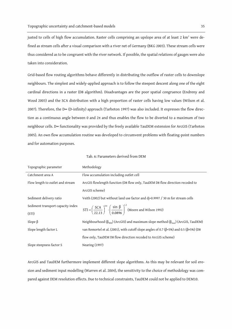
Topographic uncertainty and catchment-based models 35
justed to cells of high flow accumulation. Raster cells comprising an upslope area of at least 2 km2 were de-
fined as stream cells after a visual comparison with a river net of Germany (BKG 2003). These stream cells were
thus considered as to be congruent with the river network. If possible, the spatial relations of gauges were also
taken into consideration.
Grid-based flow routing algorithms behave differently in distributing the outflow of raster cells to downslope
neighbours. The simplest and widely-applied approach is to follow the steepest descent along one of the eight
cardinal directions in a raster (D8 algorithm). Disadvantages are the poor spatial congruence (Endreny and
Wood 2003) and the SCA distribution with a high proportion of raster cells having low values (Wilson et al.
2007). Therefore, the D∞ (D-infinity) approach (Tarboton 1997) was also included. It expresses the flow direc-
tion as a continuous angle between 0 and 2π and thus enables the flow to be diverted to a maximum of two
neighbour cells. D∞ functionality was provided by the freely available TauDEM extension for ArcGIS (Tarboton
2005). An own flow accumulation routine was developed to circumvent problems with floating-point numbers
and for automation purposes.
Tab. 6: Parameters derived from DEM
Topographic parameter Methodology
Catchment area A Flow accumulation including outlet cell
Flow length to outlet and stream ArcGIS flowlength function (D8 flow only, TauDEM D8 flow direction recoded to
ArcGIS scheme)
Sediment delivery ratio Veith (2002) but without land use factor and dj=0.9997 / 30 m for stream cells
Sediment transport capacity index
(STI)
3.16.0
0896.0βsin
13.22SCA
STI
⋅
= (Moore and Wilson 1992)
Slope β Neighbourhood (βNbh) (ArcGIS) and maximum slope method (βmax) (ArcGIS, TauDEM)
Slope length factor L van Remortel et al. (2001), with cutoff slope angles of 0.7 (β<5%) and 0.5 (β≥5%) (D8
flow only, TauDEM D8 flow direction recoded to ArcGIS scheme)
Slope steepness factor S Nearing (1997)
ArcGIS and TauDEM furthermore implement different slope algorithms. As this may be relevant for soil ero-
sion and sediment input modelling (Warren et al. 2004), the sensitivity to the choice of methodology was com-
pared against DEM resolution effects. Due to technical constraints, TauDEM could not be applied to DEM10.

36 Topographic uncertainty and catchment-based models
2.3.4 Statistics
Statistics about each topographic parameter listed in Tab. 6 were calculated for all catchments whose areas
deviated less than 25% from DEM100 (slope) or official values (other statistics). Spearman’s rank correlation
coefficients and regression equations were then determined to assess the relationships between the datasets.
Additionally, Wilcoxon tests were applied to estimate the significance of differences. Although STI and LS are
only meaningful for land areas, the stream delineation may vary according to the chosen approach (upper
catchment area threshold, SCA-slope relationship among others). Therefore, statistics were computed with
and without stream cells to obtain a general idea of dependencies on stream cell definition. All statistical anal-
yses were performed using the R-based software Statistical Lab v3.7 (FUB 2008).
2.4 Results and discussion
2.4.1 Catchment area and stream delineation
After bridge removal and manual adjustment of the gauges, the median of the ratios between modelled and
official catchment areas is close to 1.0 for all DEM and all flow algorithms. Inter-quartile ranges and the num-
ber of outliers, however, increase with raster cell size (Fig. 2). Nonetheless, individual errors occur for every
DEM and do not follow any clear trend.
Fig. 2: Modelled area to official area for different DEM resolutions and flow routing algorithms
The catchment area of each raster cell obviously depends on DEM resolution as larger raster cells also accu-
mulate more area. Consequently, with a given area threshold, the proportion of stream cells in catchments is
expected to be proportional to cell width (see Fig. 4). Nevertheless, flow routing algorithms can also have a
considerable impact (Fig. 5). The D∞ algorithm of TauDEM returns more stream cells than ArcGIS for DEM1000
(median ratio 1.37). This is not only a bifurcation effect but partly a result of flow routing in flat terrain as

Topographic uncertainty and catchment-based models 37
TauDEM’s D8 algorithm returns streams which are also 19% longer. Such areas are more prominent in the
smooth surface of DEM1000 (section 2.4.2). The differences for the other DEM are small and found to be signif-
icant for DEM50 (p<0.001) and DEM100 (p=0.02 for D∞, p=0.06 for D8). They are not significant for DEM250.
By contrast to other topographic attributes, correlation coefficients are not only relatively low between DEM
resolutions (Tab. 7) but also between flow routing algorithms. For the latter, rS values depend on DEM resolu-
tion being lowest for DEM1000 with rS≈0.6 (ArcGIS), rS<0.5 (TauDEM) and increasing to rS≈0.8 for all other DEM.
The statistical relationships are linear.
2.4.2 Slope and flow length
The highly significant increase (p<0.001) of average slope angles with DEM resolution can also be seen in Tab.
7. With raster cell sizes becoming smaller, average slopes also converge (Fig. 3 left). This pattern is similar for
both slope algorithms, although the impact is slightly lower for the maximum (D∞) than for the neighbour-
hood slope algorithm (Fig. 4). Correlation coefficients exceeding 0.9 in all cases support the inter-scale corre-
lation of average slopes observed by Wolock and McCabe (2000) and Yong et al. (2009). Linear regression mod-
els describe well the relationships, especially between fine DEM resolutions. Seven virtual gauges with
catchment means of slope angles between 10% and 35% have been included in the statistics to increase the
sample size for DEM10 and DEM50.
Fig. 3: Average slope and average flow length to streams in relation to DEM100, left: slope (βNbh), right: flow
length (ArcGIS)
Differences between slope algorithms are comparatively small and proportional to cell width (Fig. 5). They are
significant (p<0.001) for all DEM besides DEM10. The D∞ algorithm returns the highest slope angles. This is a

38 Topographic uncertainty and catchment-based models
flow routing effect because maximum slopes computed with both D8 algorithms do not differ significantly
apart from DEM250 (p=0.03). The respective coefficients of linear regression models are 1.00 (0.99 for DEM250).
Fig. 4: Effect of DEM resolution on stream delineation and average topographic attributes
Fig. 5: Method effects on stream delineation and average values of topographic attributes
Average flow lengths prove to be reciprocal to DEM cell size (Tab. 7) because flow paths meander more if grid
cells become smaller. However, the deviations are not as high as for slope angles. The relationships for flow
lengths to the outlet are linear and correlation coefficients exceed 0.98. Flow lengths to streams in DEM10 to
DEM250 behave in a similar manner, although the impact is larger and rS values are slightly smaller. In con-
trast to these DEM, flow lengths in DEM1000 are not only considerably shorter (Fig. 3 right) but they are also
moderately correlated to other DEM resolutions. These correlation coefficients are reciprocal to the propor-
tion of stream cells (Tab. 7; rS=0.65 for TauDEM D8).

Topographic uncertainty and catchment-based models 39
Tab. 7: Coefficients of regression equations y = a2x2 + a1x respectively y = a1x with x = DEM100
Neighbourhood slope Maximum slope (D∞)
Parameter DEM 10 50 250 1,000 50 250 1,000
Streams a1 0.11 0.52 2.38 6.89 0.53 2.39 9.60
n 59 63 112 91 61 108 91
rS 0.79 0.90 0.79 0.66 0.80 0.83 0.49
Slope a1 1.37 1.23 0.70 0.31 1.20 0.73 0.37
n 66 71 113 94 61 108 91
rS 0.98 0.99 0.98 0.93 0.99 0.98 0.94
Flow length to
outlet
(to streamsa)
a1 1.11 (1.16) 1.03 (1.08) 0.87 (0.88) 0.83 (0.51) 1.04 (1.09) 0.87 (0.88) 0.83 (0.21)
n 59 63 112 91 61 108 91
rS 0.98 (0.85) 0.98 (0.92) 0.99 (0.93) 0.99 (0.73) 0.98 (0.94) 1.00 (0.95) 1.00 (0.51)
STIa
(STI)
a2 0.00 0.00 0.01 0.01 0.00 0.00 0.01
a1 0.88 (0.76) 1.05 (1.11) 0.78 (0.82) 0.35 (0.27) 1.02 (1.01) 0.94 (0.92) 0.59 (0.51)
n 59 63 112 91 61 108 91
rS 0.99 (0.94) 0.99 (0.99) 0.99 (0.99) 0.93 (0.93) 1.00 (1.00) 0.99 (0.99) 0.96 (0.97)
USLE LSa
(USLE LS)
a2 0.00 0.00 0.01 0.01 0.00 0.00 0.01
a1 1.02 (1.05) 1.09 (1.11) 0.70 (0.67) 0.21 (0.19) 1.08 (1.10) 0.90 (0.86) 0.38 (0.27)
n 59 63 112 91 61 108 91
rS 0.99 (0.99) 0.99 (0.99) 0.99 (0.99) 0.93 (0.94) 0.99 (0.99) 0.99 (0.99) 0.95 (0.96)
SDRa (SDRb) a1 0.20 (0.20) 0.56 (0.23) 1.82 (2.80) 3.43 (13.92) 0.50 (0.11) 2.12 (2.59) 5.68 (22.23)
n 59 63 112 91 61 108 91
rS 0.71 (0.85) 0.97 (0.62) 0.97 (0.80) 0.87 (0.72) 0.95 (0.63) 0.92 (0.69) 0.82 (0.69)
a Non-stream cells, b TauDEM D8
The choice of methodology plays a marginal role for average slope and flow length to outlet. Flow length val-
ues are only slightly higher in TauDEM- than in ArcGIS-processed DEM. Differences are reciprocal to DEM
resolution and statistically significant (p<0.001) except for DEM1000. Correlation coefficients are above 0.99
for both parameters and linear regression models fit well (Tab. 8). In contrast, the impact is considerable for
DEM1000 when flow lengths are calculated to the streams (Fig. 5). In accordance to section 2.4.1, the correla-
tions are only moderate (Tab. 8; rS=0.76 between ArcGIS and TauDEM D8). Although the slight differences for
all other DEM are also significant (p<0.001, p=0.005 for DEM50 and D∞), rS values are higher.

40 Topographic uncertainty and catchment-based models
Tab. 8: Coefficients of regression equations y = a1x with x = ArcGIS (βNbh)
ArcGIS (βmax) TauDEM (D∞)
Parameter DEM 10 50 100 250 1,000 50 100 250 1,000
Slope a1 0.99 1.03 1.02 1.08 1.21 1.05 1.04 1.10 1.23
Flow length
(to streams)
a1 1.00
(1.00)
1.00
(1.00)
1.00
(1.00)
1.00
(1.00)
1.00
(1.00)
1.02
(0.99)
1.01
(0.98)
1.00
(0.99)
1.00
(0.40c)
STIa (STI) a1 0.93
(0.75)
0.90
(0.62)
0.93
(0.76)
0.97
(0.71)
1.38
(0.73)
0.95
(0.65)
1.00
(0.81)
1.00
(0.73)
1.45
(0.75)
USLE LSa (USLE LS) a1 0.95
(0.95)
0.95
(0.94)
0.92
(0.91)
0.91
(0.88)
1.46
(1.12)
0.97
(0.96)
0.94
(0.93)
0.91
(0.88)
1.50
(1.14)
SDRa (SDRb) a1 0.98
(0.83)
0.86
(0.53d)
0.87
(0.52)
0.93
(0.43)
1.04
(0.68)
0.76
(0.24)
0.82
(0.52d)
0.93
(0.45d)
1.39
(0.69)
a Non-stream cells, b TauDEM (D8), c rS=0.55, d 0.85<rS<0.90
2.4.3 Sediment transport capacity index (STI) and USLE LS factor
Besides the slope angle, three factors influence the dependency of both attributes on cell size changes. At first,
the DEM resolution determines the minimum possible erosive slope length and SCA. Secondly, the terrain-
smoothing effect of coarse DEM resolution (section 2.4.2) can further increase slope length values. Finally,
average slope angles decrease and so does the exponent of the L factor.
The inter-scale correlation of SCA values (Wolock and McCabe 2000; Yong et al. 2009) is supported by the high
correlation of average STI values between DEM (Tab. 7). However, the relationships between coarse and fine
DEM are not linear but slightly curved. In accordance to the equivalence of STI and the LS factor (Moore and
Wilson 1992), both attributes show a similar pattern of resolution dependency, although the impact on LS is
higher than on STI (Fig. 6 left and centre). They are also highly correlated (rS>0.99) and second-order polyno-
mial regression models describe the relationship between average LS and STI values.
The largest average values occur in DEM50, nonetheless DEM100 differs only slightly (p>0.03). The reason for
the observed drop of average STI and LS in DEM10 has to be the decrease of both SCA and erosive slope length
prevailing higher average slopes. This corresponds with observations by Sørensen and Seibert (2007) on a cell-
by-cell basis. In addition, Fig. 4 shows that values calculated by the neighbourhood slope method are stronger
influenced by DEM resolution changes, although differences to the maximum slope method decline with ras-
ter cell size. The rS values between DEM are high (Tab. 7). However, calculated values and differences are
somewhat extreme because neither land use patterns nor reasonable slope length caps were applied.
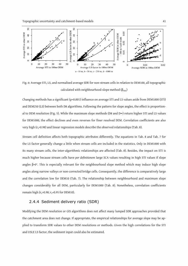
Topographic uncertainty and catchment-based models 41
Fig. 6: Average STI, LS, and normalised average SDR for non-stream cells in relation to DEM100, all topographic
calculated with neighbourhood-slope method (βNbh)
Changing methods has a significant (p<0.001) influence on average STI and LS values aside from DEM1000 (STI)
and DEM250 (LS) between both D8 algorithms. Following the pattern for slope angles, the effect is proportion-
al to DEM resolution (Fig. 5). While the maximum slope methods (D8 and D∞) return higher STI and LS values
for DEM1000, the effect declines and even reverses for finer resolved DEM. Correlation coefficients are also
very high (rS>0.98) and linear regression models describe the observed relationships (Tab. 8).
Stream cell definition affects both topographic attributes differently. The equations in Tab. 8 and Tab. 7 for
the LS factor generally change a little when stream cells are included in the statistics. Only in DEM1000 with
its many stream cells, the inter-algorithmic relationships are affected (Tab. 8). Besides, the impact on STI is
much higher because stream cells have per definitionem large SCA values resulting in high STI values if slope
angles β>0°. This is especially relevant for the neighbourhood slope method which may induce high slope
angles along narrow valleys or non-corrected bridge cells. Consequently, the difference is comparatively large
and the correlation low for DEM10 (Tab. 7). The relationship between neighbourhood and maximum slope
changes considerably for all DEM, particularly for DEM1000 (Tab. 8). Nonetheless, correlation coefficients
remain high (rS>0.98; rS=0.95 for DEM10).
2.4.4 Sediment delivery ratio (SDR)
Modifying the DEM resolution or GIS algorithms does not affect many lumped SDR approaches provided that
the catchment area does not change. If appropriate, the empirical relationships for average slope may be ap-
plied to transform SDR values to other DEM resolutions or methods. Given the high correlations for the STI
and USLE LS factor, the sediment input could also be estimated.

42 Topographic uncertainty and catchment-based models
By contrast, the distributed algorithm is inherently resolution-dependent as the number of raster cells along
each flow path increases with cell sizes becoming smaller. Therefore, the impact of changing DEM resolution
is highest among topographic attributes (Fig. 4, p<0.001). If means are corrected for cell width, they are pro-
portional to average slope. Correlation coefficients between DEM are low in comparison to other topographic
parameters (Tab. 7). The moderate values for DEM10 (0.59<rS<0.71 for ArcGIS βNbh; 0.52<rS<0.64 for ArcGIS βmax)
indicate an information content that cannot be fully explained by coarser DEM. The relationships are linear
(Fig. 6 right).
Average SDR values also change significantly if flow routing or slope calculation is altered (Fig. 5). Mostly, p is
below 0.001 except for DEM10 (p=0.01) and the D8 comparison for DEM250 (p=0.003). At a first glance, the re-
sults may contradict the slope pattern. However, higher average maximum slope angles do not mean higher
values for each raster cell. At the feet of slopes, for example, the neighbourhood slope algorithm considers the
upslope area whereas the maximum slope only includes the flatter downslope relief. Due to the shorter dis-
tance to either streams or outlet, the slope angle at a foot of slope has a higher significance than the slope
itself where maximum slope returns higher values. Terrain characteristics as well as DEM resolution deter-
mine thus the spatial pattern and absolute values of slope differences and, eventually, empirical relationships.
The considerably larger average SDR for the TauDEM-processed DEM1000 is equivalent to the larger number
of stream cells (section 2.4.1).
Without stream delineation, the raster cells next to the outlet are most important and maximum slopes are
mostly gentle here. The neighbourhood method can consider (steeper) slopes. This is more probable in coarse
DEM, given the fact that the differences between regression equations with and without stream cells are high-
er there (Tab. 8). However, the opposed trend of surface smoothing seems to partly overlay. Correlation coef-
ficients are slightly lower between both DEM resolutions and algorithms. The relationships still follow a linear
trend although the coefficients change noticeably (Tab. 7 and Tab. 8).
2.5 Conclusions
Previous studies suggested that average slope angles and SCA computed from a 100m-DEM can be downscaled
to 1,000 m resolution using linear equations (Wolock and McCabe 2000; Yong et al. 2009). Supporting these
findings, the results show that linear or slightly curved regression models are principally suitable to trans-
form catchment means of topographic attributes for DEM resolutions between 10 metres and 1,000 metres.
This is not only possible for simple but also for complex parameters such as USLE’s slope-length factor or
spatially distributed SDR. Furthermore, linear equations describe sufficiently the relations between outcomes

Topographic uncertainty and catchment-based models 43
of different single-flow routing and slope algorithms. This is important as often only one version is imple-
mented in standard GIS software. Despite significant changes in absolute values, catchment-based models are
thus capable to handle topographic uncertainty. However, there are three constraints.
Firstly, the relations are only valid as long as catchment delineation is not compromised. If catchment areas
have to be derived from a DEM, higher resolution means better conformance with official values. Discrepan-
cies here will also affect many lumped SDR approaches. Nevertheless, if DEM become too detailed artefacts
may emerge interfering with the calculation of flow directions and catchment area. Secondly, the regression
models for the spatially distributed SDR and the STI seem to be susceptible to stream definition. However, the
two tested alternatives of a constant threshold of upper catchment area for all DEM resolutions and no
streams, respectively, give only a general impression. Finally, the inter-resolution correlations are compara-
tively low for the distributed SDR approach. The moderate correlations between DEM10 and the other DEM
indicate a content being not fully explicable.
DEM and method choice significantly influences estimates of sediment or nutrient input to surface waters.
Although it is feasible to expect better results with higher DEM resolution, this study shows that this may not
be true for empirical, semi-distributed models. Pre-processing and computing time does not only increase
rapidly but benefits of better resolved DEM or elaborate algorithms are marginal. Model users may use the
proposed empirical equations to compare model results based on different DEM resolutions or topographic
algorithms. Nonetheless, an overall sensitivity analysis of sediment and nutrient models has to include other
relevant factors such as land use or soil.

3 Improving the estimation of erosion-related
suspended solid yields in mountainous, non-alpine
river catchments
Andreas Gericke & Markus Venohr (2012). Environmental Modelling & Software, 37, 30-40.
doi:10.1016/j.envsoft.2012.04.008
Received 24 October 2011, received in revised form 14 April 2012, accepted 15 April 2012
Erosion-related suspended solid yields in mountainous river catchments 45
3.1 Abstract
Sediment yields in river catchments may be modelled using a range of DEM and data algorithms. We assessed
the impact of alternative choices on the evaluation of empirical modelling approaches. The modelling frame-
work in this study consisted of the universal soil loss equation, a published local SDR, and commonly available
input data. The study area comprised the catchments of 31 monitoring gauges for which daily data of sus-
pended solids (SS) was available. For these stations, we studied the effects of two interpolation schemes for
daily SS concentrations and of two approaches to separate erosion-related ("critical") fractions from total SS
yields (SY) on model evaluation. Despite a good agreement between modelled and critical SY, the unexplained
spatial variability was considerable. For additional 109 catchments, we quantified impacts of two DEM resolu-
tions, two slope algorithms, and three slope length algorithms on modelled SY. DEM resolution and slope algo-
rithm proved to be most relevant for the model uncertainty. High correlation coefficients between the respec-
tive alternatives revealed the minor relevance of data or algorithm choices for model quality. Correlation
analyses showed that the SDR model lacked a hydrological parameter. Adjusting the modelled SDR accordingly
significantly increased the explained variability of SY.
3.2 Introduction
Human activity has significantly accelerated the natural processes of soil erosion and sediment relocation
causing global concern (Quinton et al. 2010). For surface waters, the delivery of sediments poses serious
threats to aquatic habitats and water quality, particularly because of the nutrients and pollutants attached to
the sediments (Bilotta and Brazier 2008).
In order to mitigate diffuse riverine pollution and achieve sustainable river management, estimates of sedi-
ment inputs are therefore critical. However, the underlying processes are highly variable in space and time
(González-Hidalgo et al. 2009), making monitoring in situ both complex and costly. Consequently, numerous
modelling approaches have been proposed (as reviewed by Merritt et al. 2003). With increasing computing
power and capabilities of geographical information systems (GIS), spatially distributed models have become
more able to predict runoff, soil loss and (suspended) sediment yields in river catchments. However, the per-
formance of complex, physically-based models is not necessarily better than those of empirical models, due to
process variability, parameterisation and equifinality (Jetten et al. 2003). Furthermore, the inherent variability
in replicated erosion measurements (e.g., Boix-Fayos et al. 2006) and sediment observations made Foster et al.
(2001) emphasize that it is more important to find comparative, relative estimates, than quantitatively accu-

46 Erosion-related suspended solid yields in mountainous river catchments
rate ones. For these reasons, the empirical USLE is still widely applied (Auerswald 2008), despite its conceptual
limitations (Novotny and Chesters 1989) (Eq. 1).
Generally, only a small fraction of mobilized soil particles reaches the outlet, and therefore, USLE estimates
have to be adjusted with deposition. In the simplest form, catchment-wide SDR are applied to the USLE as
correction factors. The spatial variability of such SDR has often been explained in terms of simple catchment
properties such as area or average slope (de Vente et al. 2007). This “black-box” concept has received criticism
(e.g., Novotny and Chesters 1989); however, the alternative explicit modelling of sediment flow is cumber-
some, and limited to small areas (de Vente et al. 2007). As a compromise, for larger catchments, “grey-box”
models spatially disaggregate the SDR by considering connectivity (Dymond et al. 2010) or such features as
channel distance, flow path properties, land use, and topography (e.g., Fu et al. 2010).
In this study, a modelling framework consisting of the USLE, a disaggregated SDR and (mostly) pan-European
data was used to estimate annual suspended-sediment yields for topographically diverse river catchments.
The main goal of our study was to identify the most relevant factor to improve the predictions of the empiri-
cal modelling framework. We followed the argument of Foster et al. (2001) and aimed at a relative agreement
between model results and validation data.
In this context, we quantified the implications of several data and method choices and their relevance for
(improving) the quality of model predictions. Assessing such choices is of interest because a variety of availa-
ble input data and a broad range of algorithms exist to derive model parameters, especially for topography
(e.g., Warren et al. 2004; Vaze et al. 2010). Moreover, validation data also depends on method choices (e.g.,
Phillips et al. 1999). We have focussed on three choices: i) interpolation algorithms of monitoring data of sus-
pended solids (SS), ii) algorithms to estimate the erosion-related fraction from monitoring data, iii) topo-
graphic algorithms and the DEM resolution to derive topographic parameters for the model.
The remainder of this chapter proceeds as follows. Section 3.3 briefly describes the study area. Section 3.4
presents the methods for the interpolation of SS data, the estimation of erosion-related fractions, the parame-
terisation of the USLE and the SDR including the effect of topographic representation on both model parts,
and the identification of catchment properties controlling the spatial and inter-annual variability of SS yields.
Section 3.5 discusses the quantitative and qualitative consequences of data and algorithm choices for model-
ling sediment yields and model evaluation. After presenting the controlling factors of SS variability, there is a
proposal for an improved SDR model. Chapter 3 ends with conclusions for catchment-based sediment studies.

Erosion-related suspended solid yields in mountainous river catchments 47
3.3 Study area
The study area comprised catchments of 140 gauges in the German states of Bavaria and Nordrhein-Westfalen
(NRW) (Fig. 7). These partly nested catchments also extend into other German and Austrian federal states and
small parts of the Czech Republic. The catchment areas calculated from DEM were between 19 and 25,600 km2,
with a median of 385 km2. These values agreed well with those officially reported by the State authorities.
The Bavarian gauges are located in the basins of the Danube and river Main, a tributary of the Rhine. The Dan-
ube divides the Alps and the Alpine Foothills in the south from the eastern highlands of the Bayerischer Wald
and the Fränkische Alb. The NRW catchments are situated in the North German Plain, in the basins of the
rivers Rhine, Weser and Ems. This area changes from flat, glacially sculpted landscapes in the north of NRW to
the mountainous region in the south and east.
Fig. 7: Location of the study area (NRW – Nordrhein-Westfalen)
The climate alters from maritime in the west to more continental in the east. The calculated mean annual
precipitation in the study area of 1,070 mm∙a-1 is above the typical German range from 500 mm∙a-1 to 800 mm∙a-1
(BMU 2003). The precipitation gradient from west to east is superimposed by topography. Annual values ex-
ceed 1,000 mm in highlands and 2,000 mm in the Alps.
Human activity has shaped most of the catchments and their water bodies. There are flood protection
measures and water diversion (river Altmühl), river straightening along the river Ilz, and hydropower plants
along the rivers Salzach and Isar. In NRW, mine subsidence areas are of special relevance to hydrology.

48 Erosion-related suspended solid yields in mountainous river catchments
Land use and land-use change in Bavaria and NRW are typical for Germany. Land-use distribution largely de-
pends on topography. Arable land is usually abundant in lowlands, and changes to pasture in highlands, and to
open spaces in the Alps. Since 1970, agricultural land and forests have covered about 50% and 30% of the total
study area respectively. Most of the agricultural land has been arable land with a rising proportion over the
time. Cereals are the dominant crop. In recent decades, maize has been increasingly cultivated, but root crops
less so (Destatis 1971, 1980, 1990, 2009). The expansion of maize cultivation has been associated with higher
sediment yields in the Austrian Danube basin (Summer et al. 1996). This observation is presumably also valid
for the German areas.
Tab. 9: Distribution of management strategies on arable land in 2009/10 to mitigate soil losses (Destatis 2011a;
b; Chamber of Agriculture of Upper Austria, pers. comm.)
Federal state Winter soil cover Intermediate crops Conservation tillage No-till
% % % %
Baden-Württemberg 70 20 40 1
Bavaria 60 25 20 1
NRW 80 15 30 1
Upper Austria 70a n.a. 15b n.a.
a Estimated, 35% winter grain + 35% soil cover financed by the agro-environmental programme ÖPUL, b Including no-till farming
The good agricultural practice in Germany requires a soil management that reduces soil losses, especially from
arable land. The most common management strategy in the study area is to cover soils during winter (Tab. 9).
Less relevant measures can, however, be of regional importance. For instance, intermediate crops are grown
on almost half of the arable land in the mountainous south of Bavaria (Bavarian State Office for Statistics and
Data Processing, pers. comm.) and mulching is common for maize and in the Tertiärhügelland (Tertiary Hills)
where the risk of soil loss is highest (Bavarian State Research Centre for Agriculture, pers. comm.). In NRW,
winter soil cover and conservation tillage are most abundant in the south-east (IT.NRW State Office for Infor-
mation and Technology, pers. comm.). Comparable data was not available for Austria. Nonetheless, arable land
is scarce in the Austrian sub-catchments and soil losses from there are less important for sediment yields.
3.4 Methods
3.4.1 Introduction
The modelling framework consisted of two parts. First, a combination of USLE and distributed SDR was applied
to estimate long-term average sediment yields. We evaluated how well the model explained the spatial varia-

Erosion-related suspended solid yields in mountainous river catchments 49
bility within the study area. Second, hydrological data was related to suspended-solid yields to explain the
inter-annual SS variability.
To describe the implications of data and method choices for the model outcome and model quality, we corre-
lated the alternative long-term averages among all catchments to assess the spatial variability and alternative
annual values for each catchment to assess the temporal variability. We assumed that a high correlation coef-
ficient indicates that the choice is of less importance for the explained variability, i.e. a poor model perfor-
mance cannot be attributed to an unfavourable choice but to limitations of the USLE or the SDR model. For
this case, we used correlation analyses to identify catchment properties to improve model predictions. In con-
trast, a low correlation coefficient implies that the model performance can be improved by a careful choice.
The estimation of erosion-related fractions, the modelling framework, and identification of controlling factors
and the statistical analyses are presented in this chapter. Statistical analyses were performed using the soft-
ware package R 2.10.1 (R Development Core Team 2009).
3.4.2 Estimation of critical yields of suspended solids (SS)
3.4.2.1 Monitoring data on suspended solids
Daily values of SS concentration (SSC) and water discharge (Q) for 31 monitoring stations were provided by
the Bavarian Environment Agency (Table 2). SSC and Q have mostly been monitored for 20–30 years. The time
series of SSC were interpolated from single point measurements taken with buckets at irregular intervals. The
sampling frequency depended on flow conditions and typically ranged from multiple samples per day to one
sample a week. Multi point measurements were occasionally carried out to calibrate and validate the standard
routine (all information from LfU 2000).
The Bavarian Environment Agency has adopted two different methods (henceforth method A and B) to inter-
polate daily means from the sampling data. In method A, the concentration SSCi measured or linearly interpo-
lated (Eq. 2) at time ti (in hours) was time-weighted using the trapezoidal rule (Eq. 3).
i1i1i
1i1ii Q
QQSSCSSC
SSC ⋅++
=+−
+− Eq. 2
[ ] [ ]( )∑=
++ −⋅+⋅=n
1ii1i1iiA ttSSCSSC5.0
241
SSC Eq. 3
n is the number of trapezoids covering one day (SSC values at midnight were also linearly interpolated). In
method B, the trapezoidal rule was similarly applied to interpolate SS loads as product of SSCi and Qi instead of
50 Erosion-related suspended solid yields in mountainous river catchments
SSCi. If one sampling was taken at a day, Qi was the daily mean value. Otherwise, Qi was interpolated at time ti
(in seconds). SSCB was the ratio of daily average SS load and daily Q.
Occasionally there were small gaps in the SSC data, which we filled by linear interpolation (Q ≈ const.) or esti-
mated from the sampling data taken at these days. For most monitoring stations, the results of both interpola-
tion alternatives were available, thus we assessed the consequences of method choice on suspended solid
yields for model evaluation.
Mean specific runoff q of the gauges and intra-annual dynamics were closely related to topography (Tab. 10).
Accordingly, the rivers were categorized into non-alpine (lowlands and highlands) and alpine. Alpine rivers
were typically found to have peaks of runoff and sediment yield during late spring and summer because of the
combined effect of melting snow and summer precipitation. In contrast, most non-alpine rivers had their
minimum of q and SS yields (SY) in these seasons due to increased evapotranspiration. However, a few catch-
ments did not clearly fit into either group. The intra-annual dynamics were extenuated by lakes, dams and
barrages for the rivers Mindel, Amper and Isar.
3.4.2.2 Estimation of critical SS yields
Monitoring gauges necessarily integrate all SS sources and processes within their catchments. Although soil
erosion is the main source of suspended solids in Bavaria (Habersack et al. 2008), comparing model outcomes
to total yields (e.g., Auerswald 1992) would generally overestimate its contribution. In order to evaluate an
erosion-based model, it is necessary to estimate the erosion-related fraction from an observed total SY. This
genuine inverse task is challenging because no simple relationship exists between SS dynamics and other
processes within rivers and river catchments (Sivakumar and Jayawardena 2003).
Assuming that non-eroded fractions (e.g., phytoplankton, industrial effluents) are almost independent of wa-
ter discharge, the erosion-related (henceforth “critical”) fraction was estimated for each gauge using long-
term average SS concentrations and loads for discharge classes following Behrendt et al. (1999) (Fig. 8). In
most cases, SSC and loads increased considerably above a gauge-specific critical discharge Qcrit. To obtain Qcrit,
Q was first quantized using varying bin widths. For each bin, the average values for Q, SSC and SS load were
calculated and linear regression models were developed for low Q (RMlow) and high Q (RMhi) to predict SSC and
SS loads from Q. Qcrit was determined as the intersection of RMlow and RMhi. Critical yields are the difference
between RMhi and RMlow for Q>Qcrit. In other words, RMlow is the base load SYbase not related to soil erosion. In
this study, SYgraph refers to the critical yields of this graphical-statistical approach.

Erosion-related suspended solid yields in mountainous river catchments 51
Tab. 10: Overview of gauges for validation, collection periods and basic catchment properties, H – average
height, β – average slope, Ar – arable land (Corine Land Cover 2000), Pr – interpolated long-term average an-
nual precipitation (section 3.4.3.3.1), and q – measured average annual runoff
Gauge River Area H βd Ar Pr q Availability
km² m % % mm∙a-1 mm∙a-1 (q and SY)
Aha Altmühl 693 453 4.0 55 781 192 1976–1999
Bad Kissingen Fränk. Saale 1,572 382 8.1 53 820 267 1974–2003
Burghausene Salzach 6,649 1,268 36.8 3 1,422 1,205 1970–2002
Coburg Itz 346 455 10.6 40 979 466 1991–2002
Dietldorf Vils 1,100 465 7.3 39 843 308 1988–2003
Duggendorf Naab 5,434 504 7.3 38 854 299 1971–2003
Gemünden Sinn 610 431 14.2 13 991 401 1984–2003
Harburg Wörnitz 1,569 475 5.2 58 856 247 1988–2003
Hohenkammer Glonn 390 504 4.0 73 965 263 1971–2003
Hüttendorf Regnitz 3,864 422 6.2 40 805 253 1989–2003
Inkofen Amper 3,076 622 6.1 37 1,132 489 1971–2003
Kalteneck Ilz 760 714 13.0 8 1,209 682 1971–2003
Kemmern Main 4,224 433 9.3 44 891 336 1971–2003
Kemptene Iller 955 1,182 30.4 4 1,754 1,539 1971–2003
Laufermühle Aisch 956 342 5.4 57 738 171 1971–2003
Mainleus Main 1,166 481 9.1 43 932 408 1993–2003
Muggendorf Wiesent 660 465 7.8 54 934 344 1971–2003
Neumühle Rednitz 1,847 424 5.3 42 775 226 1990–2001
Oberaudorfe Inn 9,715 1,809 45.7 1 1,240c 985 1971–2003
Offingen Mindel 949 597 4.8 27 1,040 426 1970–2003
Pettstadt Regnitz 6,991 404 6.4 46 812 246 1971–2003
Plattlinga Isar 8,435 741 13.5 34 1,199 658 1970–2003
Regenstaufb Regen 2,658 593 12.2 22 1051 463 1972–1991
Ruhstorf Rott 1,052 447 5.5 76 933 287 1971–2003
Schärdinge Inn 25,664 1,204 30.2 15 1,218 903 1971–2003
Schlehenmühleb Roter Main 71 488 6.1 33 904 269 1978–1992
Schönachb Große Laber 407 419 4.9 72 790 196 1989–1992
Steinbe Traun 367 852 23.7 5 1,779 1,074 1971–1992
Taferlruckab Große Ohe 19 1,003 18.6 0 1,265 977 1983–1992
Unterjettenbergbe Saalach 927 1,213 42.8 0 1,693 1,262 1971–1992
Vilsbiburgb Große Vils 320 484 4.9 81 946 282 1972–1992
a Intra-annual runoff pattern similar to alpine catchments, b Only SSCB data available (section 3.4.2.1) c Adjusted (section 3.4.3.3.1), d Neighbourhood approach, e Alpine catchment, f Calculated with Corine Land Cover (2000)

52 Erosion-related suspended solid yields in mountainous river catchments
Fig. 8: Estimation of critical yields of suspended solids according to Behrendt et al. (1999). Average SS concen-
trations (triangles) and SS loads (circles) for Q intervals were used to establish regression models for high and
low Q. The critical yield SYgraph for each gauge was derived from the difference between both regression mod-
els for SS concentrations (broken lines) and SS loads (straight lines).
SSCB values (section 3.4.2.1) were used to compare SYgraph estimates to estimates obtained with the “functional
streamflow disaggregation” (FSD) technique (Carl and Behrendt 2008). In FSD, total discharge is seen as super-
position of conceptual runoff components. This data-sparing method was originally used to decompose time
series of daily discharges from headwater catchments (Carl et al. 2008). The components were found to rea-
sonably approximate classical overland flow, interflow, and base flow as generated by distributed hydrological
models, though a range of uncertainty remained in these tentative assignments.
FSD code version 1.0 (Carl 2009) was used to estimate the overland flow Qfast by the “fast” FSD component.
Very small negative values were – as round-off artefacts (P. Carl, pers. comm.) – set to zero. For technical rea-
sons, the time series were split into subsets of 11 years maximum. Possible boundary effects were avoided
using an overlap of 2 years. SYFSD, the alternative to SYgraph, was finally obtained as the product of qfast and SSCB
with qfast = Qfast∙A-1. The term “critical SY” subsumes SYgraph and SYFSD throughout this study.
3.4.2.3 Evaluation of verification data
For both algorithms for interpolation and critical-yield estimation, we compared the spatial variability of
long-term average critical SY and the annual values for single gauges. Histograms and Kolmogorov-Smirnov
tests showed that the data was not normally distributed. Thus the non-parametric Spearman rank correlation
coefficient (rS) was calculated to assess qualitative differences. Additionally, Wilcoxon tests were conducted to
test whether quantitative differences between alternatives were significant. The null hypothesis was rejected
if p≥0.05. To obtain quantitative differences, we calculated the slope of the regression model y = a1x.

Erosion-related suspended solid yields in mountainous river catchments 53
To our knowledge, no established inverse method exists to derive critical yields from total SS yields. Valida-
tion was not possible but we modified the algorithm for SYgraph to assess the plausibility of results and to ex-
plore differences between critical SY. Three modifications were applied for gauges with i) high dissimilarity
between average SYFSD and SYgraph, ii) low correlation of annual values, and iii) large discrepancy to model re-
sults (section 3.3.5). First, bin widths for Q quantization were calculated from quantiles to assess the effect of
alternative binning on SYgraph estimates (SYalt_bin). Second, the alternative SYtot_base was calculated as the differ-
ence between total SY and the regression model for low Q (SYbase) to overcome possible limitations of the line-
ar regression model for high Q. Third, SYgraph was calculated for single years to better reflect the inter-annual
variability of sediment yields (SYann_graph).
3.4.3 Modelling approach
3.4.3.1 Model outline
Sediment yields were modelled using raster datasets. The geometric resolution of the raster DEM was set as
reference for all other input data. All GIS operations were performed with ArcGIS 9.2 (Esri 2006). The main
steps consisted of i) defining streams as a prerequisite for the distributed sediment delivery ratio (SDR), ii)
estimating the USLE factors and soil loss, and iii) estimating the SDR. For each non-stream raster cell, gross
soil erosion and the SDR were calculated to estimate the amount of eroded soil that eventually reaches the
stream network and the outlet. For stream cells, it was assumed that no soil loss occurs. Long-term in-stream
deposition was also neglected because no information was available that would allow parameterisation. Simi-
lar to the USLE estimates, sediment yields (SY) as a product of SDR and USLE soil loss were long-term annual
means.
3.4.3.2 Deriving the stream network
For defining the starting points of the stream network, we adopted the approach of Colombo et al. (2007). The
study area was subdivided into 3 regions according to precipitation, lithology, relief, vegetation cover, and
soils. For each region, we analysed the relationship between local slope (β) and specific catchment area to
define the minimum catchment area for stream initiation. Raster cells with catchment areas between 1.1 and
1.4 km2 were defined as starting points. Additionally, surface curvature was considered to include visible line-
ar surface features like small rivers and valleys. It was assumed that surface runoff is dominantly linear here
and thus the USLE is not valid.
The D8 algorithm as proposed by Jenson and Domingue (1988) was applied for flow routing and subsequent
stream delineation from raster DEM. This algorithm was readily implemented in the ArcGIS software package.

54 Erosion-related suspended solid yields in mountainous river catchments
It exclusively assigns the outflow of a raster cell to the raster cell along the steepest descent in its 3x3 neigh-
bourhood. The streams were combined with water bodies taken from the Corine Land Cover 2000 dataset
(CLC2000) (EEA 2007a). Artificial waterways were not considered.
3.4.3.3 Estimating soil erosion
USLE factors were estimated using coarse datasets and empirical approaches (Tab. 11). Coarse resolution does
not only refer to geometry but to content as well. For instance, the European Soil Database (ESBN and EC 2004)
contained 6 texture classes instead of specific percentages for silt, clay and sand. Therefore, all factors were
estimated with empirical relationships which have been published for the study area or which are widely
accepted. As several approaches have been suggested in the literature for the L factor, the consequences of
choices were exemplarily assessed.
Tab. 11: Overview of methods and data to estimate USLE factors (β – slope angle)
Factor Dataset Data (Resolution) Method Reference (Method)
R Long-term average pre-
cipitation (Pr, mm∙a-1)
Points (Variable;
0.5° raster)
RBavaria = 0.078 ∙ Pr + 4.3 Strauss and Blum (1994)
RNRW = 0.1096 ∙ Pr – 14.25 DIN (2005)
K European Soil Database Polygons (1:1 Mio) K = 0.0086 ∙ silt% + 0.0083 Strauss et al. (2003)
C∙P CLC2000; agricultural
statistics
Polygons
(1:100,000; admin-
istrative units)
C = f(land use) and P = 0.85
for arable land
Kagerer and Auerswald
(1997); Auerswald (2002);
Stumpf and Auerswald (2006) C constants and P = 1.0
L∙S SRTM-DEM (Jarvis et al.
2006); DEM (NRW Sur-
veying and Mapping
Agency)
Raster (100 me-
tres; 50 metres) βsin1.63.2e1
175.1S ⋅−++−= Nearing (1997)
Iterative L factor van Remortel et al. (2001)
L = f(β) Asselman et al. (2003); Fuchs
et al. (2010)
3.4.3.3.1 R factor
A raster dataset of long-term average annual precipitation (Pr) was interpolated from calibrated annual data
obtained from the German Meteorological Service (DWD) and monthly data from the Global Precipitation
Climatology Centre (GPCC), using an inverse distance weighting algorithm. To improve interpolation across
the Alps and Austria, we included stations for which only long-term means were available (1961–1990, 1971–
2000) (DWD, Austrian Central Institute for Meteorology and Geodynamics). The uncalibrated DWD data (Pruncal)

Erosion-related suspended solid yields in mountainous river catchments 55
was adjusted to altitude H (in metres) using a linear relationship (Eq. 4, Behrendt unpubl.). R factors were
estimated from this dataset applying specific empirical relationships for NRW and Bavaria / Austria (Tab. 11).
uncalPr63H 0.0525Pr ++⋅= Eq. 4
The results of our approach were tested for plausibility because station density was low for Austria. Pr and
runoff q fitted well for all catchments except the alpine Oberaudorf which lies largely in Austria. This was
confirmed by an independent raster dataset (HISTALP) (Efthymiadis et al. 2006; ZAMG 2009). Therefore, we
changed our Pr value of 1,028 mm∙a-1 to the more realistic HISTALP value (Tab. 10).
3.4.3.3.2 K factor
For each soil typological unit, the soil database provided information on the dominant surface textural class
(attribute TEXT1). The class value was translated to silt content according to van der Knijff et al. (2000).
3.4.3.3.3 C∙P factor
According to Auerswald (2002), statistical information on land use was evaluated to determine the percentage
of small grain and sod-forming crops for administrative units (Tab. 12). Information on the percentage of root
crops in mulch-tillage systems was scarcely available. This value was set to 2.5% in NRW (Schmidt et al. 2007)
and to 0% elsewhere. The C value was assigned to all arable land and heterogeneous agricultural areas within
an administrative unit (CLC2000 codes 21x and 24x). These C factors were spatially disaggregated because C
factors are i) much higher for arable land than for other land uses and thus more important for soil loss in
river catchments and ii) largely dependent on crops and crop rotation schemes.
For some raster cells in Bavaria, we found a combination of arable land on very steep slope angles which ex-
hibits a high risk of soil loss. We assumed this combination to be unlikely and to be the result of inaccuracies
in the input data (e.g., the minimum mapping unit of CLC2000 of 25 ha is above the DEM resolution). Land use
classes 21x and 24x were thus replaced by pasture (CLC class 231) on slope angles above 25% (Strauss 2007).
Tab. 12: Statistical data on land-use used to determine C factors for arable land
Region Spatial domain Year Data source
Austria Federal state 1999 Statistik Austria
Bavaria, Baden-Württemberg, Thüringen County 2003 State Offices for Statistics
Czech Republic Region (kraj) 2003 Czech Statistical Office
Nordrhein-Westfalen (NRW) County 2004 Chamber of Agriculture

56 Erosion-related suspended solid yields in mountainous river catchments
3.4.3.3.4 L∙S factor
The SRTM-DEM was transformed to 100 metres raster resolution. Bridges which affected water flow routing
and catchment delineation in flat terrain were removed from the 50m-DEM using a simple GIS-based approach
(section 2.3.2).
Slope angles for the S factor and the SDR were computed with the maximum (βmax) and a neighbourhood
method (βNbh). The latter is the standard plane-fit algorithm as implemented in the ArcGIS software package.
We compared three L factors. First, we used a regression model between βNbh (in °) and L factors measured in
the German Federal State of Baden-Württemberg (Eq. 5) (Fuchs et al. 2010). Second, the L factor was derived
from a constant erosive slope length of 100 metres following Asselman et al. (2003) and Liu et al. (2000) (Eq. 6).
Third, we applied the iterative GIS algorithm proposed by van Remortel et al. (2001) (LGIS). For LGIS, erosive
slope lengths were separately computed from slope changes along flow routes for CLC2000 classes. The upper
limit was set to 3 raster cells (300 metres), the maximum of Lemp. For forests, a maximum of LGIS = 2 was defined
(Stumpf and Auerswald 2006).
3038.1β729.0β0937.0β0028.0L Nbh2Nbh
3Nbhemp +⋅+⋅−⋅= Eq. 5
1bb
m100 m13.22m100L
+
= with ( )56.0βsin30896.0
βsinb 8.0 +⋅⋅= Eq. 6
3.4.3.4 Estimating sediment yields (SY)
Sediment delivery to streams was calculated for each raster cell as a product of long-term soil erosion and the
sediment delivery ratio (SDR). A modified SDR approach of Halbfaß and Grunewald (2008) was applied, approx-
imating the land use factor α with the C factor (Eqs. 7–8).
{ } iiLLi E1,LβamaxSY ⋅⋅= Eq. 7
( ) 49.9Cln43.1α ii +⋅= Eq. 8
For each raster cell i, the original local land use factor αi and slope βi were replaced by the downslope averages
Lα and Lβ to represent flow path characteristics. These averages were calculated by summing up all values αi
and βi along the flow path and dividing the sum by the length Li of the flow path.

Erosion-related suspended solid yields in mountainous river catchments 57
All variables in the equation above refer to the centres of non-stream cells. Local SDR of raster cells next to
stream cells below 5% indicated a low probability of sediment transfer into stream cells. The upslope areas of
such cells and of urban areas were excluded.
3.4.3.5 Verifying soil erosion, sediment yields and sediment delivery ratios
Sediment sources other than sheet and rill erosion are sensu stricto outside the scope of the chosen model ap-
proach. This is certainly the case for alpine catchments where landslides and stream erosion are important
processes (Tab. 10). Model evaluation was therefore only possible for non-alpine catchments. Among those
catchments, total sediment yields measured at Schlehenmühle (Roter Main) and Kalteneck (Ilz) were extraor-
dinary high (SYtot=42 Mg∙km-2∙a-1). This is due to urban runoff at Schlehenmühle (Strohmeier et al. 2005) and an
alpine-like character of the river Ilz and its tributaries (R. Brandhuber, pers. comm.). For all other catchments,
former studies showed that the USLE is sufficient to estimate sediment yields.
Modelled soil loss was indirectly verified by applying the empirical SDR equations proposed by Auerswald
(1992) and Behrendt et al. (1999) to the USLE results. Both SDR equations were originally calibrated with Ba-
varian SS monitoring data similar to our dataset. To test the agreement of modelled soil erosions, regression
analyses were conducted. In accordance to the methods and data used in both studies, the products of SDR and
USLE results were compared to total SS load and SYgraph.
Linear regression models (y = a1x) were applied to evaluate the different modelled sediment yields and SDR.
The slope a1 was used as a measure for average quantitative differences to critical SY and SDR. The signifi-
cance of a1=1.0 (match) was obtained with t-tests. The adjusted r2 were calculated as a measure of how well the
models explain the quasi-observed variability of critical SY.
“Critical SDR” values were calculated as ratio of critical SY to modelled soil erosion. They were correlated to
modelled SDR in order to assess whether the USLE or the SDR approach failed to capture the spatial variability
in the study area. Similar to the verification of evaluation data (section 3.4.2.3), Spearman’s rank correlation
was conducted for correlation analyses. Weak correlations between modelled and critical SY suggest that the
empirical approaches for the USLE factors or the USLE itself were inappropriate while weak correlations for
SDR indicate the need for improving the SDR approach.

58 Erosion-related suspended solid yields in mountainous river catchments
3.4.3.6 Analysing topographic uncertainty
The regression models used for model evaluation were also used to quantify the topographic uncertainty.
Correlation coefficients were evaluated to assess whether method choices or DEM resolution affect the ex-
plained variability of the verification data.
3.4.4 Improving model results
3.4.4.1 Variability of sediment yields (SY)
To complement the model structure, correlation analyses were conducted to identify catchment-wide control-
ling factors of critical-SY and SDR variability. Our reasons for this approach were two-fold. First, the available
data resolution limits the cell-based SDR approach to land use and terrain. However, there are many more
environmental and anthropogenic factors which influence hydraulic connectivity and sediment delivery.
Second, the USLE only returns average annual values of soil loss. Nonetheless, it is well-known that SY and SSC
can vary considerably over time, as a combination of variability in soil loss and sediment transport. A small
number of events can contribute large fractions of annual yields, and their role may even be enhanced by
reservoir flushing (e.g., Hamm and Glassmann (1995) for the river Salzach). However, their distribution and
frequency may not be well related to annual precipitation used in the present study to estimate USLE R factors
(Auerswald 1992).
Only a few studies in the Bavarian and Austrian river catchments have related environmental and anthropo-
genic factors such as geology, flow distance, water discharge (Bauer 1967), land use and land use change
(Summer et al. 1996), power plants (Weiss 1996) to sediment variability. Auerswald (1992) analysed total SS for
22 Bavarian catchments and proposed a linear relationship to annual R factors, catchment area and soil loss.
Behrendt et al. (1999) also developed a linear model for the inter-annual variability of SY.
3.4.4.2 Identifying factors controlling the variability of suspended solids
We tested the strength and significance of correlations between possible controlling factors (Tab. 13) and the
set of critical SY and SDR. All but the climatic and hydrological factors were considered to be static. We ana-
lysed the spatial variability of long-term average SSC and SY among the catchments. For climatic and hydro-
logical factors, annual values were calculated to analyse the temporal variability for each catchment. Because
the SDR was defined as the ratio of SY and long-term mean soil erosion, the inter-annual variability of critical
SY and critical SDR were identical. The statistical methods were similar to those mentioned in sections 3.4.2.3
and 3.4.3.5.

Erosion-related suspended solid yields in mountainous river catchments 59
Tab. 13: Catchment properties (possible controlling factors) which were correlated to critical SY and SDR (see
Restrepo et al. (2006) for definitions and references)
Factor group Factors
Land use Proportion of urban areas, arable land, pasture, forests and open spaces (%)
Average distance of agricultural land to streams (lagri, km)
Morphometry Catchment area (A, km2)
Average slope (β, %)
Average, minimum and maximum height (H, Hmin, Hmax, m)
Catchment length (LC, km)
River length (LR, km)
Drainage density (DD, km∙km-2)
(H-Hmin)/(Hmax-Hmin) (HI, -)
H/A (β1, m∙km-1)
H/Hmax (Hpk, -)
Hmax/LC (Hr, m∙km-1)
Erosion E (Mg∙km-2∙a-1) and USLE factors
Climate and Hydrology Annual and long-term average Qtot, Qfast (m3∙s-1)
Annual and long-term average Qtot/A (qtot, mm∙a-1), qfast
Annual precipitation (Prann, mm∙a-1) and Pr (mm∙a-1)
Prann/PrM 1970–2003 (PP, -)
Modified Fournier index 1970–2003 (MFI, mm∙a-1)
Annual and long-term average SSC (kg∙m-3)
Mixed β∙C, H∙Ar, H∙Pr
Annual precipitation data was not available for all stations. Additional steps were thus necessary to estimate
annual catchment means of precipitation (Prann). They were calculated by first interpolating GPCC data and
DWD stations for which annual sums of precipitation were available (Pr’ann). Pr’ann and its long-term mean Pr’
was applied to derive Prann from the long-term precipitation Pr already used for the USLE R factor (section
3.4.3.3.1) (Eq. 9). Similarly to Pr, we used the HISTALP dataset to test for plausibility. The inter-annual variabil-
ity of both precipitation datasets was found to be consistent for each gauge (rS ≈ 0.9).
For the calculation of the Modified Fournier index (MFI) (Arnoldus 1980), average maximum monthly precipi-
tation (PrM) was estimated similarly to Prann by first interpolating monthly GPCC data (PrM, GPCC). PrM, GPCC and the
annual sum (PrGPCC) were applied to calculate PrM from Prann (Eq. 10).

60 Erosion-related suspended solid yields in mountainous river catchments
{ }rPrPmeanPrPr annann ′′⋅= Eq. 9
{ }GPCCGPCC,MannM PrPrmeanPrPr ⋅= Eq. 10
We regressed annual values of critical SY to annual values of the climatic and hydrological factors to explain
their inter-annual variability. The regression analysis not only aimed at finding the highest explained variabil-
ity for all monitoring gauges but also to test the regression models for a more general applicability. To achieve
this, the regression model for each gauge was compared to the regression model for all other gauges. In each
case, we used t-tests to test the null hypothesis H0 that the exponents of both regression models do not differ
significantly. The fewer the rejections of H0 were, the more suitable for a broader application the global re-
gression model was considered.
3.5 Results and discussion
3.5.1 Evaluation of validation data
3.5.1.1 Interpolation of daily average SS concentration
The interpolation of daily data from irregular monitoring was the basis for the estimation of (critical) SS yields
and model evaluation. Sampling frequency is always a trade-off between an adequate description of the natu-
ral SS variability and the cost for sampling and analysis. However, large deviations between both interpolation
algorithms occurred during measurement gaps close to events with high SY and low SSC (Fig. 9) or inversely.
Fig. 9: Interpolation method and sampling interval (vertical lines at the bottom), gauge Hohenkammer
For model evaluation, the algorithm choice of the data provider had a significant (p<0.0001) though variable
impact on interpolated SSC. Long-term and monthly means revealed 7% higher SSC values for interpolation
method B than A with individual differences ranging from 1% to >20%. Significant and almost identical devia-
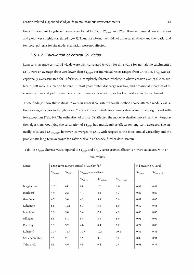
Erosion-related suspended solid yields in mountainous river catchments 61
tions for resultant long-term means were found for SYtot, SYgraph, and SYFSD. However, annual concentrations
and yields were highly correlated (rS≥0.9). Thus, the alternatives did not differ qualitatively and the spatial and
temporal patterns for the model evaluation were not affected.
3.5.1.2 Calculation of critical SS yields
Long-term average critical SS yields were well correlated (rS=0.87 for all, rS=0.76 for non-alpine catchments).
SYFSD were on average about 25% lower than SYgraph, but individual ratios ranged from 0.4 to 1.8. SYFSD was ex-
ceptionally overestimated for Taferlruck, a completely forested catchment where erosion events due to sur-
face runoff were assumed to be rare. In most years water discharge was low, and occasional increases of SS
concentrations and yields were merely due to base load variations, rather than soil loss in the catchment.
These findings show that critical SY were in general consistent though method choice affected model evalua-
tion for single gauges and single years. Correlation coefficients for annual values were usually significant with
few exceptions (Tab. 14). The estimation of critical SY affected the model evaluation more than the interpola-
tion algorithm. Modifying the calculation of SYgraph had mostly minor effects on long-term averages. The an-
nually calculated SYann_graph, however, converged to SYFSD with respect to the inter-annual variability and the
problematic long-term averages for Taferlruck and Kalteneck, further downstream.
Tab. 14: SYgraph alternatives compared to SYgraph and SYFSD, correlation coefficients rS were calculated with an-
nual values
Gauge Long-term average critical SY, Mg∙km-2∙a-1 rS between SYFSD and
SYgraph SYFSD SYgraph alternatives SYgraph SYann_graph
SYalt_bin SYtot_base SYann_graph
Burghausen 110 64 98 101 134 0.87 0.87
Dietldorf 4.9 2.2 4.4 4.0 4.7 0.82 0.87
Gemünden 6.7 3.0 6.3 5.3 5.6 0.49 0.65
Kalteneck 5.8 10.6 6.3 5.5 8.9 0.80 0.68
Mainleus 3.9 3.8 3.4 2.5 4.3 0.46 0.83
Offingen 5.5 5.1 5.4 5.3 6.9 0.91 0.92
Plattling 5.1 3.7 4.8 4.4 7.2 0.77 0.83
Ruhstorf 11.7 11.9 11.7 10.4 10.4 0.86 0.85
Schlehenmühle 37 26 32 32 34 0.85 0.94
Taferlruck 0.5 4.6 0.5 0.4 2.4 0.61 0.37

62 Erosion-related suspended solid yields in mountainous river catchments
3.5.2 Evaluation of model results
3.5.2.1 Soil erosion
We considered our catchment-wide soil losses to be consistent with those used by Auerswald (1992) and
Behrendt et al. (1999). Applying their SDR models to soil loss and comparing the modelled SY to total SY
(Auerswald 1992) and SYgraph (Behrendt et al. 1999) gave slopes of linear regression models close to 1.0. Alt-
hough input data, temporal coverage, and the calculation of USLE factors slightly differed, r2 values of 0.62 and
0.91 were also similar to, or even above, those published. Deviations were systematic. For instance, the under-
estimation of about 15% when applying Auerswald’s approach occurred due to the USLE P factor of 0.85 for
arable land in our study instead of 1.0. The soil losses were not evaluated for four catchments for which we
assumed that critical SY values did not match the erosive fraction of total SY (next section).
3.5.2.2 Sediment yields and sediment delivery ratios
Correlations between area-specific soil erosion and critical SY were suspiciously weak for non-alpine catch-
ments (cf. Tab. 17). Four gauges played an important role but no common explanation could be found. Most
plausible reasons are SS sources outside the scope of the USLE that both disaggregation methods were unable
to separate (urban runoff, in-stream erosion), sediment retention (not included in the SDR approach) and one
very short, not representative time series. Without these gauges, correlation coefficients increased to rS≥0.7
for SYgraph, but remained lower for SYFSD (0.5≤rS<0.7).
Tab. 15: Regression models between alternative modelled and critical SY obtained for the 100m-DEM, model
y = a1x with modelled SY as y and critical SY as x, t-tests used to test for the significance of a1 ≠ 1.0
Critical SY Modelled SY
βNbh βmax βNbh
LGIS L100m LGIS L100m Lemp
SYA, graph a1 1.49** 1.40** 1.09 1.08 1.47***
r2 (b) 0.59 0.59 0.61 0.64 0.69
SYB, graph a1 1.28* 1.21 0.94 0.94 1.30**
r2 (b) 0.51 0.52 0.51 0.56 0.65
SYaFSD
a1 1.40* 1.33* 1.02 1.05 1.50**
r2 (b) 0.39 0.37 0.37 0.40 0.56
a Without gauges at Taferlruck, Dietldorf, Bad Kissingen (see text for details) b For intercept ≠ 0, *** p<0.001, ** p<0.01, * p<0.05
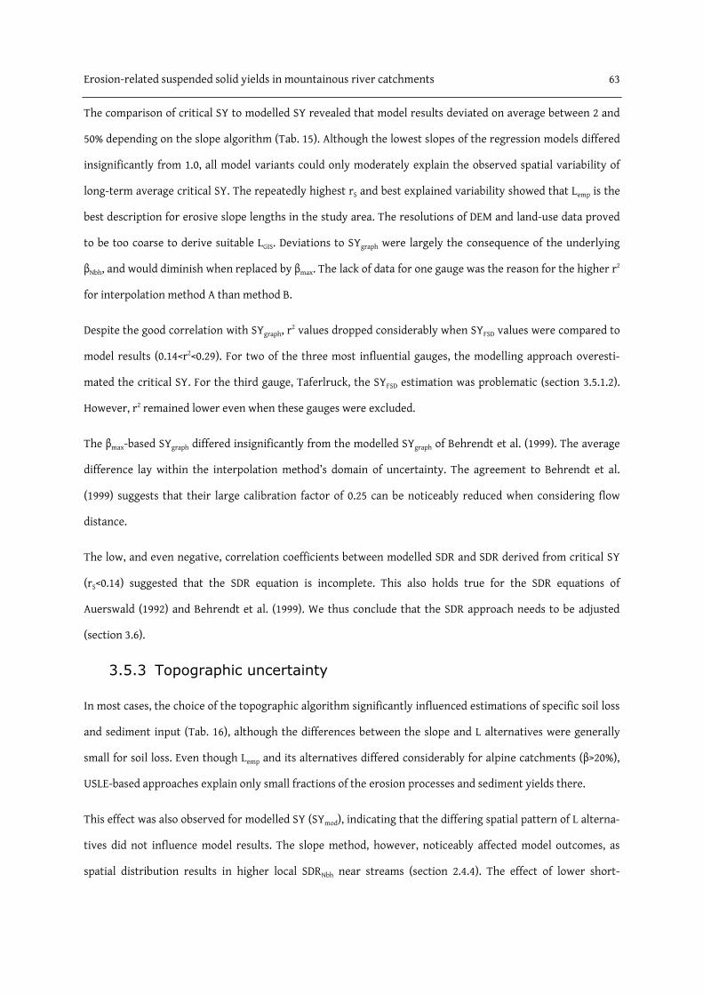
Erosion-related suspended solid yields in mountainous river catchments 63
The comparison of critical SY to modelled SY revealed that model results deviated on average between 2 and
50% depending on the slope algorithm (Tab. 15). Although the lowest slopes of the regression models differed
insignificantly from 1.0, all model variants could only moderately explain the observed spatial variability of
long-term average critical SY. The repeatedly highest rS and best explained variability showed that Lemp is the
best description for erosive slope lengths in the study area. The resolutions of DEM and land-use data proved
to be too coarse to derive suitable LGIS. Deviations to SYgraph were largely the consequence of the underlying
βNbh, and would diminish when replaced by βmax. The lack of data for one gauge was the reason for the higher r2
for interpolation method A than method B.
Despite the good correlation with SYgraph, r2 values dropped considerably when SYFSD values were compared to
model results (0.14<r2<0.29). For two of the three most influential gauges, the modelling approach overesti-
mated the critical SY. For the third gauge, Taferlruck, the SYFSD estimation was problematic (section 3.5.1.2).
However, r2 remained lower even when these gauges were excluded.
The βmax-based SYgraph differed insignificantly from the modelled SYgraph of Behrendt et al. (1999). The average
difference lay within the interpolation method’s domain of uncertainty. The agreement to Behrendt et al.
(1999) suggests that their large calibration factor of 0.25 can be noticeably reduced when considering flow
distance.
The low, and even negative, correlation coefficients between modelled SDR and SDR derived from critical SY
(rS<0.14) suggested that the SDR equation is incomplete. This also holds true for the SDR equations of
Auerswald (1992) and Behrendt et al. (1999). We thus conclude that the SDR approach needs to be adjusted
(section 3.6).
3.5.3 Topographic uncertainty
In most cases, the choice of the topographic algorithm significantly influenced estimations of specific soil loss
and sediment input (Tab. 16), although the differences between the slope and L alternatives were generally
small for soil loss. Even though Lemp and its alternatives differed considerably for alpine catchments (β>20%),
USLE-based approaches explain only small fractions of the erosion processes and sediment yields there.
This effect was also observed for modelled SY (SYmod), indicating that the differing spatial pattern of L alterna-
tives did not influence model results. The slope method, however, noticeably affected model outcomes, as
spatial distribution results in higher local SDRNbh near streams (section 2.4.4). The effect of lower short-

64 Erosion-related suspended solid yields in mountainous river catchments
distance SDR (b100=1.19, b50=1.07) was enhanced by excluding more upstream areas when βmax was applied
(b100=1.35, b50=1.14).
Tab. 16: Correlation coefficients rS and linear regression models y = a1x for modelled soil loss and sediment
yield calculated with topographic alternatives. *indicate the significance of differences (Wilcoxon tests)
Correlated pair of values βNbh - βmax L100m - LGIS Lemp - LGIS 50 m - 100 m (LGIS)
Alternatives LGIS
(50 m)
LGIS
(100 m)
L100m βNbh βmax βNbh βNbh βmax
Soil loss (E)
Mg∙km-2∙a-1
p ** *** *** *** - - (***a) *** ***
rS 1.00 1.00 1.00 0.99 0.99 0.91 0.99 0.99
a1 0.98 1.02 0.97 0.93 0.97 0.97 1.22 1.28
Sediment yield
(SYmod)
Mg∙km-2∙a-1
p *** *** *** *** - * (-a) *** ***
rS 1.00 0.99 0.99 0.99 0.99 0.96 0.95 0.95
a1 1.14 1.35 1.29 0.92 0.96 0.95 1.88 2.23
a β≤20% (non-alpine catchments), *** p<0.001, ** p<0.01, * p<0.05, - not significant at the 5% level
Increasing the DEM resolution raised soil loss estimates by more than 20% (LGIS). The minor effect of shorter
erosive slope lengths and lower L factors (-8%) was dominated by higher slope angles. For Lemp and L100, the
dependency on DEM resolution was thus even more pronounced. The effects of DEM resolution on SYmod were
distinctly higher than on soil loss because of the denser drainage network in the 50m-DEM, resulting in short-
er flow distances. Similar to chapter 2, the high correlation coefficients showed that topographic choices are
of minor relevance for model quality except for the L factor (sections 2.4 and 3.5.3). This result also agrees
with other observations (Wu et al. 2005; de Vente et al. 2009).
3.6 Improving model results
3.6.1 Controlling factors of spatial variability
The correlation analysis of the whole dataset revealed that SSC and qfast almost equally well explained the
distribution of long-term average SY (Tab. 17). Topography superimposes the relationship between catchment
area A and SYtot observed in many other studies. Steep slopes, high precipitation, and a large fraction of open
spaces make alpine catchments effective sediment suppliers, independent of their area. Consequently, the
correlations were strong for SYtot (rS>0.8) and catchment properties like the proportion of open space, average
height (H), and precipitation (Pr) when assessing the whole dataset. This also held true for the SDR because
the USLE underestimates soil loss in such catchments. Due to the high correlations, method choices had minor
effects on correlation coefficients (except for the USLE L factor).
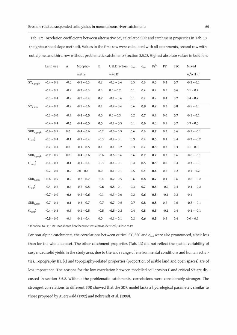
Erosion-related suspended solid yields in mountainous river catchments 65
Tab. 17: Correlation coefficients between alternative SY, calculated SDR and catchment properties in Tab. 13
(neighbourhood slope method). Values in the first row were calculated with all catchments, second row with-
out alpine, and third row without problematic catchments (section 3.5.2). Highest absolute values in bold font
Land use A Morpho-
metry
E USLE factors
w/o Ra
qtot qfast Prb PP SSC Mixed
w/o H∙Prc
SYB, graph -0.4 – 0.5 -0.0 -0.3 – 0.5 0.2 -0.3 – 0.6 0.5 0.6 0.6 0.4 0.7 -0.3 – 0.1
-0.2 – 0.1 -0.2 -0.3 – 0.3 0.3 0.0 – 0.2 0.1 0.4 0.2 0.2 0.6 0.1 – 0.4
-0.3 – 0.4 -0.2 -0.2 – 0.4 0.7 -0.1 – 0.6 0.1 0.2 0.2 0.4 0.7 0.4 – 0.7
SYB, FSD -0.4 – 0.3 -0.2 -0.2 – 0.6 0.1 -0.4 – 0.6 0.6 0.8 0.7 0.3 0.8 -0.5 – 0.1
-0.3 – 0.0 -0.4 -0.4 – 0.5 0.0 0.0 – 0.3 0.2 0.7 0.4 0.0 0.7 -0.1 – 0.1
-0.4 – 0.4 -0.6 -0.4 – 0.5 0.5 -0.1 – 0.5 0.1 0.6 0.3 0.2 0.7 0.3 – 0.5
SDRB, graph
(LGIS)
-0.6 – 0.5 0.0 -0.4 – 0.6 -0.2 -0.6 – 0.5 0.6 0.6 0.7 0.3 0.6 -0.5 – -0.1
-0.3 – 0.4 -0.1 -0.1 – 0.4 -0.3 -0.4 – 0.1 0.3 0.4 0.5 0.1 0.4 -0.3 – -0.2
-0.2 – 0.1 0.0 -0.1 – 0.5 0.1 -0.1 – 0.2 0.3 0.2 0.5 0.3 0.3 0.1 – 0.3
SDRB, graph
(Lemp)
-0.7 – 0.5 0.0 -0.4 – 0.6 -0.6 -0.6 – 0.6 0.6 0.7 0.7 0.3 0.6 -0.6 – -0.1
-0.4 – 0.3 -0.1 -0.1 – 0.4 -0.3 -0.4 – 0.1 0.4 0.5 0.5 0.0 0.4 -0.3 – -0.1
-0.2 – 0.0 -0.2 0.0 – 0.4 0.0 -0.1 – 0.1 0.5 0.4 0.6 0.2 0.2 -0.1 – 0.2
SDRB, FSD
(LGIS)
-0.6 – 0.5 -0.2 -0.2 – 0.7 -0.4 -0.7 – 0.5 0.6 0.8 0.7 0.1 0.6 -0.6 – -0.2
-0.4 – 0.2 -0.4 -0.2 – 0.5 -0.6 -0.5 – 0.1 0.3 0.7 0.5 -0.2 0.4 -0.4 – -0.2
-0.7 – 0.0 -0.6 -0.2 – 0.6 -0.3 -0.3 – 0.0 0.2 0.6 0.5 -0.1 0.2 -0.1
SDRB, FSD
(Lemp)
-0.7 – 0.4 -0.1 -0.3 – 0.7 -0.7 -0.7 – 0.6 0.7 0.8 0.8 0.2 0.6 -0.7 – -0.1
-0.4 – 0.3 -0.3 -0.2 – 0.5 -0.5 -0.5 – 0.2 0.4 0.8 0.5 -0.1 0.4 -0.4 – -0.1
-0.5 – 0.0 -0.4 -0.1 – 0.4 0.0 -0.1 – 0.1 0.2 0.6 0.5 0.2 0.4 0.0 – 0.2
a Identical to Pr, b MFI not shown here because was almost identical, c Close to Pr
For non-alpine catchments, the correlations between critical SY, SSC and qfast were also pronounced, albeit less
than for the whole dataset. The other catchment properties (Tab. 13) did not reflect the spatial variability of
suspended solid yields in the study area, due to the wide range of environmental conditions and human activi-
ties. Topography (H, β1) and topography-related properties (proportion of arable land and open spaces) are of
less importance. The reasons for the low correlation between modelled soil erosion E and critical SY are dis-
cussed in section 3.5.2. Without the problematic catchments, correlations were considerably stronger. The
strongest correlations to different SDR showed that the SDR model lacks a hydrological parameter, similar to
those proposed by Auerswald (1992) and Behrendt et al. (1999).

66 Erosion-related suspended solid yields in mountainous river catchments
3.6.2 Controlling factors of temporal variability
The water discharge (Q) better explained critical SY values than the annual precipitation (Pr), Modified Four-
nier Index (MFI) or suspended-solids concentration (SSC) (Fig. 10, Tab. 18). Although the estimated surface
runoff Qfast was the best parameter from which to predict critical SY, it is more feasible under most circum-
stances to use precipitation instead. This merely practical aspect was supported by t-tests that showed overall
models to be more representative when Pr was the explanatory variable. The comparison of gauge-specific
and general regression models revealed that both exponents differed significantly in only one case for Pr-
based but considerably more often for Q-based and MFI-based models. Despite larger deviations, Pr is thus
more suitable for regional applications than is Qfast, while the lower residuals for Qfast are advantageous when
focusing on specific gauges.
Fig. 10: Correlation coefficients for individual monitoring gauges between annual values of potential control-
ling factors and SS yields. Wilcoxon test performed for paired controlling factors. Significance shown if p<0.05
A visual analysis revealed that power equations were more suitable regression models than formerly proposed
linear equations between hydrological parameters and SY (Auerswald 1992; Behrendt et al. 1999). Nonetheless,
the generally high residuals (Tab. 18) show the limitations of aggregated values to explain the inter-annual
variability of (critical) SY in this environmentally diverse study region. The highest exponents and residual
standard deviations of regression models for SYgraph reveal the disproportionate scatter of annual values in
comparison to SYtot and SYFSD.

Erosion-related suspended solid yields in mountainous river catchments 67
It is important to note that all regression models clearly underestimated the SY values for a few station-years,
mainly flood years in alpine catchments. Floods often occur during short time periods, thus more detailed
input data is necessary to predict such extreme events. Additionally, such simple regression models cannot
consider monitoring gaps during flood events and reservoir flushing (river Salzach in 1991) or sudden increas-
es in SSC with constant Q due to works or collapsing banks (river Aisch, May 1983, M. Knott, pers. comm.).
Tab. 18: Regression models for critical annual SY compared to total SY for comparison (upper row for all
catchments and lower row for non-alpine catchments). Power equations were derived by nonlinear least
squares fitting
x SYFSD SYgraph SYtot
Pr 0.95∙x2.89 (σ=0.56) 0.84∙x4.80 (σ=0.68) 0.98∙x2.19 (σ=0.37)
0.94∙x2.91 (σ=0.52) 0.81∙x4.95 (σ=0.60) 0.97∙x2.19 (σ=0.34)
MFI 0.97∙x2.54 (σ=0.59) 0.92∙x3.74 (σ=0.76) 0.99∙x1.90 (σ=0.40)
0.96∙x2.42 (σ=0.56) 0.91∙x3.69 (σ=0.73) 0.98∙x1.82 (σ=0.38)
Qfast 0.99∙x1.26 (σ=0.46) 0.95∙x1.62 (σ=0.63) -
0.99∙x1.19 (σ=0.41) 0.94∙x1.60 (σ=0.57) -
Qtot 0.98∙x1.70 (σ=0.57) 0.91∙x2.78 (σ=0.61) 0.99∙x1.45 (σ=0.34)
0.97∙x1.68 (σ=0.51) 0.89∙x2.79 (σ=0.52) 0.99∙x1.40 (σ=0.30)
3.6.3 Adjusting the sediment delivery ratio (SDR)
The moderately explained spatial variability proved the limitations of the modelling framework (Tab. 15).
Irrespective of quantitative differences between the alternative model results, the high correlation coeffi-
cients demonstrated that, especially for topography, data and algorithm choices would not help to lessen this
unexplained variability. An exception is the empirical approximation of the USLE L factor (Lemp) which proved
to be superior to both alternative approaches. Nonetheless, strong correlations also showed that empirical,
catchment-based models can efficiently cope with topographic uncertainty by including simple regression
models. According to the correlation analyses (Tab. 17), a hydrological catchment property was included in
the SDR model (Eqs. 11–12).
( )19n%,10SDR,46.0r95.0qSDR011.0SDR emp2
fastempemp,cor =<=+⋅⋅= Eq. 11
( )78.0r55.0SY90.0SY 2graph,Bemp,cor =+⋅= Eq. 12

68 Erosion-related suspended solid yields in mountainous river catchments
The adjusted SDR values for non-alpine catchments were between 2.5 and 6.8%. The inverse correlation to
catchment area (rS=-0.24) was stronger than for the original SDR (Fig. 11). The explained variability increased
significantly even though one gauge was included which was excluded before. The average deviation for the
Lemp-based SY estimates decreased from +30% (Tab. 15) to -3%. This lay within the degree of uncertainty due to
the interpolation methods for SS data. For large-scale applications, qfast can be replaced by Pr. Results similarly
improved for SYFSD. The r2 value rose significantly even with the inclusion of three gauges not previously con-
sidered (r2=0.64) and average deviation was also -3%.
The remaining unexplained variability and the model residuals have to be seen in the model scope which did
not include the numerous anthropogenic activities, long-term deposition and other discharge-dependent
sediment sources. In accordance with findings of Wu et al. (2005), the inherent limitations of the empirical
modelling framework may not allow for much more accuracy.
Fig. 11: Adjusted SDR and modelled SDR for non-alpine catchments (SDR modelled with Lemp as USLE L factor
and SYgraph)
The hydrological catchment property used for model improvement can be considered as proxy for catchment-
wide hydraulic connectivity. Precipitation and surface runoff are not only driving forces of soil mobilization
but also of sediment transport. With this adjustment, catchments receiving more precipitation or having more
surface runoff are not only prone to more soil loss but to a higher proportion of sediment leaving the catch-
ment as well. However, we are aware that the need for the hydrological adjustment also refers to our estima-
tion of the USLE R factor, despite the successful verification of the modelled soil erosion. This concerns the
interpolation of long-term average precipitation as well as the suitability of the linear empirical equations to
estimate the R factor from long-term annual precipitation.

Erosion-related suspended solid yields in mountainous river catchments 69
3.7 Conclusions
We have demonstrated that established empirical approaches for soil erosion and sediment delivery, in com-
bination with Europe-wide available input data, can sufficiently explain the spatial pattern of long-term aver-
age yields of the erosion-related (critical) fractions of total suspended solid yields in hilly and mountainous
catchments in southern Germany. To achieve a better explained variability of sediment yields in the study
area, it was necessary to include a hydrological catchment property in the SDR approach. We expect that this
modelling framework can also be applied in other European regions. Land use, flow distance (drainage densi-
ty), hydrology (precipitation), and topography are commonly available for river catchments and thus suitable
to estimate catchment-wide sediment delivery ratios in large-scale studies. However, within such modelling
framework, multiple algorithms and DEM are available for derivation of topographic parameters and creation
of validation data. Each alternative has a significant quantitative influence on topographic parameters, model
estimates and validation data, respectively.
Our findings revealed that among these choices, DEM resolution had the largest impact on modelled soil ero-
sion and sediment yields, with scale effects on slope angles and drainage density being most important. Model
estimates were also strongly related to the choice of the slope algorithm with results differing by 30% between
the neighbourhood and the maximum slope method. This value was close to the average deviation of 25%
between both approaches to obtain critical fractions of total yields for model validation.
We also found that the estimation of critical yields affected the prediction of the inter-annual variability of
sediment yields. Unlike the spatial variability, the mathematically-founded FSD approach gave better results
than the alternative graphical approach. However, our aggregated hydrological parameters only moderately
explained the inter-annual variability. Although we used power equations instead of formerly proposed linear
regression models, extremely high sediment yields were still clearly underestimated. More detailed input data
are needed to improve predictions for flood years.
The inherent limitations of the empirical modelling framework, and coarse data resolution, may impede de-
termination of which alternative algorithm is superior. The range of relationships between model outcomes
and validation data has to be seen as methodical uncertainty. Nonetheless, high correlation coefficients of
long-term averages and annual critical suspended solid yields in most cases showed that the tested algorithms
and DEM resolutions alone have only minor impacts on the explained variability of critical yields.
The erosion estimates were consistent with other studies. However, the calculated critical SDR were uncorre-
lated to our and other modelled SDR. Correlation analyses between critical SDR and catchment properties

70 Erosion-related suspended solid yields in mountainous river catchments
revealed that empirical SDR models should consider hydrology (surface runoff, precipitation). Consequently,
including our estimated surface runoff significantly improved the model evaluation.
Although this study discussed the consequences of method choices for an USLE context in a complex region,
the identified principles are also relevant for other modelling frameworks and regions. First, the estimation of
total and subsequently critical sediment yields will affect any model calibration and validation. However, our
observed similarity is limited to different interpolation approaches and may not be valid for different meas-
urement methods and sampling frequencies. Second, the qualitative similarity of even complex topographic
parameters suggests that catchment-based models can use regression models for any region to handle topo-
graphic uncertainty. Third, calibrating erosion models to total suspended solids overestimates the contribu-
tion of soil erosion. We recommend using critical yields instead and applied two approaches to estimate such
critical sediment yields from daily monitoring data. In general, the results were consistent and methodical
modifications were of minor relevance. However, the data-sparing and easy-to-use FSD approach agreed less
to the spatial pattern of modelled long-term sediment yields but described the inter-annual variability of
critical yields much more reasonably than the alternative graphical-statistical approach.
From our findings, we propose three topics for future studies. First, an improved estimation of the USLE R
factor would make the SDR adjustment more reliable. Second, some ambiguous results and gauge-specific
problems suggest that both approaches to derive erosion-related fractions from suspended-solids data should
be further scrutinized. Third, the very high sediment yields of flood years have to be better captured.

4 Modelling the inter-annual variability of sediment
yields: A case study for the upper Lech River
Nazzareno Diodato, Andreas Gericke & Gianni Bellocchi (2012). Catena, 97, 12-19.
doi:10.1016/j.catena.2012.04.013
Received 4 December 2011, received in revised form 21 April 2012, accepted 28 April 2012

72 Inter-annual variability of sediment yields, Lech River
4.1 Abstract
Pulsing storms and prolonged rainfall events have been associated to floods, soil erosion and nutrient fluxes in
many European river catchments. This motivated us to develop a parsimonious approach to model the climate
forcing on sediment yields in a mountainous Austrian-German river catchment. The hydro-climatologic forc-
ing was interpreted by the novel RAMSES (RAinfall Model for SEdiment yield Simulation) approach to estimate
the annual sediment yields. We used annual data on suspended-solid yields at the gauge Füssen, monitored
from 1924 to 2003, and monthly rainfall data. The dataset was split into the period 1924–1969 for calibration
and the period 1970–2003 for validation. The quality of sediment yield data was critically examined, and a few
outlying years were identified and removed from further analyses. These outliers revealed that our model
underestimates exceptionally high sediment yields in years of severe flood events. For all other years, the
RAMSES performed well against the calibration set, with a correlation coefficient (r) equal to 0.83 and a Nash-
Sutcliffe model efficiency (ME) of 0.69. The lower performance in the validation period (r=0.61, ME=0.36) has to
be partly attributed to discontinuities in the monitoring strategy. For the calibration dataset, monthly precipi-
tations proved nonetheless to be better predictors for annual sediment yields than annual values. These first
results lay the foundation for reconstructing intra- to inter-decadal variability of sediment yields in river
catchments where detailed precipitation records are not available as well as for the reconstruction of histori-
cal sediment yields.
4.2 Introduction
Understanding how climate forcing affects basin-wide responses is crucial not only for erosion and sediment
modelling but also for the reconstruction of hydro-geomorphological hazards (Higgitt 2001; Angel et al. 2005).
Climate and flow regime played key roles in the mobilisation and relocation of sediments in river basins
(Walling and Fang 2003; Piégay et al. 2004; Macklin et al. 2006; Verstraeten et al. 2009). This was already docu-
mented in historical times, as scientists understood the erosion phenomena by empirical observations. For
instance, Leonardo Da Vinci wrote in his “Treatise on Water” (1489): “The sediment of the rivers are more
abundant in areas that are densely populated … where the places, the mountains and hillslopes are tilled and
the rain sweeps away more easily a ploughed soil than a soil that is hard and covered by vegetation”
(translation by Pfister et al. 2009, p. 14).
Sediment yield is the amount of eroded soil exported over given time and space units. The underlying pro-
cesses of soil erosion, sediment transport and deposition have been well described (e.g., Morgan 1986; Rose

Inter-annual variability of sediment yields, Lech River 73
1993; Haan et al. 1994) and many methods have been designed to assess soil erosion and sediment transport
and the variability at different spatial and temporal scales (as reviewed by Brazier (2004) and Gao (2008)).
The many factors which control soil detachment and transport make sediment yields highly variable in space
and time. Many empirical relationships have been proposed to relate the spatial variability to catchment
properties (e.g., de Vente et al. 2007) because explicit modelling is demanding and not necessarily superior to
empirical approaches (Jetten et al. 2003). Hydraulic connectivity and features such as channel distance, land
use, and topography have been used to spatially disaggregate the sediment delivery of river catchments (e.g.,
Lenhart et al. 2005; Dymond et al. 2010; Fu et al. 2010).
The temporal variability is bound to rainfall power and overland flow, which trigger soil detachment and
transportation. In many cases, a few large events contribute significantly to multi-year sediment yields
(González-Hidalgo et al. 2010). Against the background of climate change, shifts in rainfall intensity and storm
events are expected to affect future soil erosion and sediment yields (Wei et al. 2009). Annual sediment yields
are usually weakly related to annual precipitation (Wilson 1973; Auerswald 1992). The inter-annual variability
has been attributed to water discharge and climate pattern (Restrepo and Kjerfve 2000), the annual rainfall-
runoff erosivity factor R of the USLE (Auerswald 1992), and heavy rainfall events (Lamoureux 2000). Welsh et
al. (2009) even used a cellular automata model to simulate changes in the hydrological and sediment regime
over 180 years at an hourly time step. However, the access to long records of water discharge and (sub-)daily
input rainfall data for modelling is critical, and such data are only available for a few, geographically-scattered
stations (e.g., Diodato and Bellocchi 2010).
This calls for parsimonious approaches for river catchments or time spans where the rainfall data are limited.
Several simple empirical relationships between the R factor and commonly available factors have already
been established (as, for instance, in Diodato and Bellocchi (2010)), mostly annual precipitation or simple indi-
ces based on monthly values. However, these factors may not sufficiently reflect the seasonal pattern of sedi-
ment processes like snowmelt in spring and thunderstorms in summer. Therefore, our aim was to develop and
test an approach which i) explains the inter-annual and inter-decadal variability of sediment yields with a few,
simple climate and land-use factors and ii) recognises seasonal and monthly precipitation associated with
different sediment processes. Such an approach is necessarily unable to capture the details of individual sedi-
ment-forming fluxes.
We hypothesised that the monthly rainfall pattern is a better predictor for annual sediment yields than annu-
al hydrological values. The novel model called RAMSES (RAinfall Modelling for SEdiment yield Simulation) was
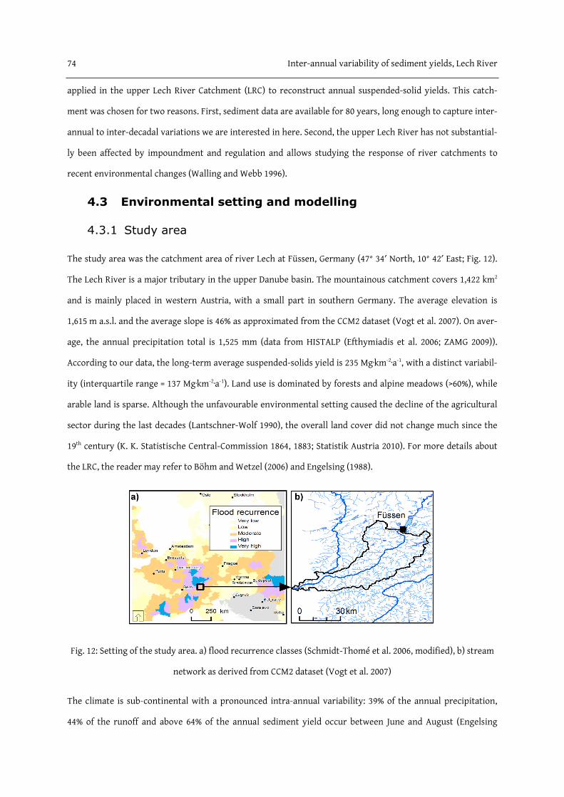
74 Inter-annual variability of sediment yields, Lech River
applied in the upper Lech River Catchment (LRC) to reconstruct annual suspended-solid yields. This catch-
ment was chosen for two reasons. First, sediment data are available for 80 years, long enough to capture inter-
annual to inter-decadal variations we are interested in here. Second, the upper Lech River has not substantial-
ly been affected by impoundment and regulation and allows studying the response of river catchments to
recent environmental changes (Walling and Webb 1996).
4.3 Environmental setting and modelling
4.3.1 Study area
The study area was the catchment area of river Lech at Füssen, Germany (47° 34′ North, 10° 42′ East; Fig. 12).
The Lech River is a major tributary in the upper Danube basin. The mountainous catchment covers 1,422 km2
and is mainly placed in western Austria, with a small part in southern Germany. The average elevation is
1,615 m a.s.l. and the average slope is 46% as approximated from the CCM2 dataset (Vogt et al. 2007). On aver-
age, the annual precipitation total is 1,525 mm (data from HISTALP (Efthymiadis et al. 2006; ZAMG 2009)).
According to our data, the long-term average suspended-solids yield is 235 Mg∙km-2∙a-1, with a distinct variabil-
ity (interquartile range = 137 Mg∙km-2∙a-1). Land use is dominated by forests and alpine meadows (>60%), while
arable land is sparse. Although the unfavourable environmental setting caused the decline of the agricultural
sector during the last decades (Lantschner-Wolf 1990), the overall land cover did not change much since the
19th century (K. K. Statistische Central-Commission 1864, 1883; Statistik Austria 2010). For more details about
the LRC, the reader may refer to Böhm and Wetzel (2006) and Engelsing (1988).
Fig. 12: Setting of the study area. a) flood recurrence classes (Schmidt-Thomé et al. 2006, modified), b) stream
network as derived from CCM2 dataset (Vogt et al. 2007)
The climate is sub-continental with a pronounced intra-annual variability: 39% of the annual precipitation,
44% of the runoff and above 64% of the annual sediment yield occur between June and August (Engelsing
Inter-annual variability of sediment yields, Lech River 75
1988). For May to August, these values increase to 50–80%. The yearly and seasonal variability is the result of
snow melt and of the synoptic circulation that advects air masses of different origins. This dynamic effect is
strongly modulated by the Alps (Holton 2004). Air masses allow high storage of humidity that represents the
main energy supply for thunderstorms, which are triggered by outbreaks of Atlantic polar maritime air in the
middle troposphere.
Floods have been common in the LRC (Böhm and Wetzel 2006) (Fig. 12a) and have sometimes been severe (e.g.,
in 1910, 1999, 2002). Scheurmann and Karl (1990) provide a brief overview of the many flood protection mea-
surements that were carried out in the upper Lech catchment. Nonetheless, the river partly maintained its
natural wildness (Scheurmann and Karl 1990; Hettrich and Ruff 2011). In this region, the most extreme storm
events are induced by instabilities produced by the frontal air masses brought from the North Atlantic, which
result in both summer and early autumn precipitation maxima (e.g., Heino et al. 1999). This circulation pat-
tern can be associated both with prolonged rainfall-driven large floods and sediment yield and intensive rain-
storm-driven flash floods and intermediate floods with accelerated soil erosion (e.g., Diodato 2006). Large
floods are accompanied by continuous runoff with great transport capacity of sediment at the basin outlet.
Intermediate floods are suitable to remove great masses of soil that do not entirely arrive at the outlet, while
net erosion driven by flash floods is negligible. In such Alpine catchments, snow melt can further increase
runoff and sediment yield. In the LRC, the severe floods in 1910 and 1999 were the consequence of snowmelt
and heavy rainfall (Meier 2004).
4.3.2 Data source
Annual values of runoff and total suspended solids were provided by the Bavarian Environment Agency for
the years 1924–2003. They are similar to those discussed by Walling (1997). We used the HISTALP dataset to
obtain monthly values of precipitation (Efthymiadis et al. 2006; ZAMG 2009). Information on land use was
taken from the Corine Land Cover 2006 map (EEA 2010c) and statistical yearbooks.
Sediment data in Bavaria are measured as suspended solids. These are single-point measurements, which are
occasionally calibrated and validated with multi-point measurements. The sampling frequency depends on
water discharge. Samples are taken several times a day during runoff events or otherwise irregularly (daily to
weekly). The average daily sediment yield is calculated from linearly interpolated daily suspended sediment
concentrations and daily water discharge. More recently, the algorithm was changed to interpolating sedi-
ment loads directly, with considerable uncertainties when measurement gaps occurred next to flood events
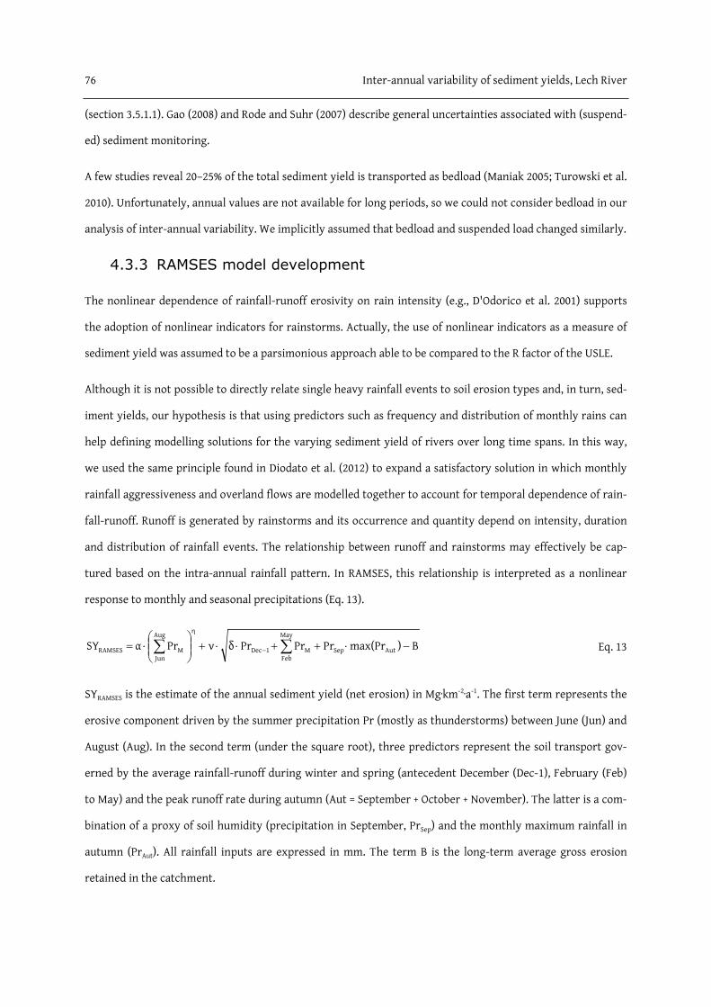
76 Inter-annual variability of sediment yields, Lech River
(section 3.5.1.1). Gao (2008) and Rode and Suhr (2007) describe general uncertainties associated with (suspend-
ed) sediment monitoring.
A few studies reveal 20–25% of the total sediment yield is transported as bedload (Maniak 2005; Turowski et al.
2010). Unfortunately, annual values are not available for long periods, so we could not consider bedload in our
analysis of inter-annual variability. We implicitly assumed that bedload and suspended load changed similarly.
4.3.3 RAMSES model development
The nonlinear dependence of rainfall-runoff erosivity on rain intensity (e.g., D'Odorico et al. 2001) supports
the adoption of nonlinear indicators for rainstorms. Actually, the use of nonlinear indicators as a measure of
sediment yield was assumed to be a parsimonious approach able to be compared to the R factor of the USLE.
Although it is not possible to directly relate single heavy rainfall events to soil erosion types and, in turn, sed-
iment yields, our hypothesis is that using predictors such as frequency and distribution of monthly rains can
help defining modelling solutions for the varying sediment yield of rivers over long time spans. In this way,
we used the same principle found in Diodato et al. (2012) to expand a satisfactory solution in which monthly
rainfall aggressiveness and overland flows are modelled together to account for temporal dependence of rain-
fall-runoff. Runoff is generated by rainstorms and its occurrence and quantity depend on intensity, duration
and distribution of rainfall events. The relationship between runoff and rainstorms may effectively be cap-
tured based on the intra-annual rainfall pattern. In RAMSES, this relationship is interpreted as a nonlinear
response to monthly and seasonal precipitations (Eq. 13).
B)max(PrPrPrPrδνPrαSY AutSep
May
FebM1Dec
ηAug
JunMRAMSES −⋅++⋅⋅+
⋅= ∑∑ − Eq. 13
SYRAMSES is the estimate of the annual sediment yield (net erosion) in Mg∙km-2∙a-1. The first term represents the
erosive component driven by the summer precipitation Pr (mostly as thunderstorms) between June (Jun) and
August (Aug). In the second term (under the square root), three predictors represent the soil transport gov-
erned by the average rainfall-runoff during winter and spring (antecedent December (Dec-1), February (Feb)
to May) and the peak runoff rate during autumn (Aut = September + October + November). The latter is a com-
bination of a proxy of soil humidity (precipitation in September, PrSep) and the monthly maximum rainfall in
autumn (PrAut). All rainfall inputs are expressed in mm. The term B is the long-term average gross erosion
retained in the catchment.

Inter-annual variability of sediment yields, Lech River 77
The empirical parameters α, δ and η express the rainfall power within the climatic context. The coefficient ν is
a vegetation exponential function describing the protection by land cover (Eq. 14, after Thornes (1990)). LVC is
the land vegetation cover, and γ and ζ are two empirical parameters.
LVCζeγν ⋅−⋅= Eq. 14
4.3.4 Model evaluation
The dataset was split for model calibration (1924–1969) and model validation (1970–2003). Several statistical
tests were applied to evaluate the agreement between RAMSES estimates and actual sediment values. First, the
Pearson’s correlation coefficient r and r2 were calculated to assess the linear dependence between modelled
and observed data and the variance explained by the model. Second, the Nash-Sutcliffe model efficiency (ME)
(Nash and Sutcliffe 1970) and the mean absolute error (MAE) were derived to assess quantitative differences.
For perfect models, MAE is 0 and ME is 1. Poor models have high MAE (up to +∞) and low ME (down to -∞).
Third, the Durbin-Watson test (Durbin and Watson 1950, 1951) was conducted to test for autocorrelated resid-
uals because strong temporal dependence may induce spurious correlations (Granger et al. 2001). All analyses
were performed with STATGRAPHICS Online (StatPoint Technologies 2012).
We also compared the RAMSES to three simplified approaches (Eqs. 15–17). Pr is the annual precipitation
(mm), MFI is the Modified Fournier index (FAO and UNEP 1977), and q is the total annual runoff (l∙s-1∙km-2).
Precipitation model bPM PraSY ⋅= Eq. 15
MFI model bMFI MFIaSY ⋅= with ∑
=
=12
1M
2M
PrPr
MFI Eq. 16
Runoff model bq qaSY ⋅= Eq. 17
These models have been developed in chapter 3 to describe the inter-annual variability of sediment yields in
the same region between the 1970s and 2003. Their runoff model was slightly superior in explaining the varia-
bility of sediment yields, although catchment-specific regression models differed significantly. All models
failed to predict the extraordinary high sediment yields of some flood years in alpine catchments (section
3.4.4.2).

78 Inter-annual variability of sediment yields, Lech River
4.4 Results and discussion
In this section, the comparison between measured sediment yield (SY) and RAMSES results is presented and
discussed. The concept and the assumptions of RAMSES are discussed for its applicability beyond the study
area.
4.4.1 Model parameterization and evaluation
Equations 13 and 14 were parameterized according to Tab. 19. A few observations were dropped from further
analyses because of very high residuals (Fig. 13a). For the calibration dataset, we observed suspicious values
for 1934, 1936, 1945, 1956, 1960 and 1965 but found no common explanation.
Tab. 19: Values assigned to parameters of Eqs. 13 and 14
Equation Parameter Value Source
13 α 0.625 Calibration
η 1 Calibration
δ 50 Calibration
B 235 Calibration
14 γ 170 Calibration
ζ 0.07 Thornes (1990)
LVC 81 Statistical yearbooks
Fig. 13: Analysis for the calibration and validation datasets. a) scatterplot between predicted and observed
sediment yields (Mg∙km-2∙a−1) for the calibration dataset with bounds of 95% prediction limits (grey curves),
frequency distributions on both axes, 1:1 line (grey) and the line of best fit (black). The regression was calcu-
lated without the outliers (grey), a1) distribution of residuals, a2) comparison of theoretical to sample quantiles
(QQ-plot), b) scatterplot for validation dataset similar to a)

Inter-annual variability of sediment yields, Lech River 79
We assumed that the sediment yield and the precipitation values for 1945 were affected by the (post-)war
situation. In 1965, late snow-melt together with high rainfall led to a major flood in June (e.g., Embleton-
Hamann 2007). For that year, RAMSES underestimated the very high sediment yield. For the four other outli-
ers, the precipitation in June was above the third quartile of the whole dataset while winter precipitation was
below average (Fig. 14). This indicates that the model in a few cases overemphasises the effect of the precipita-
tion in early summer or during the winter on sediment yields.
Fig. 14: Monthly precipitation regime for the Lech catchment (1924–2003) (box plots) compared to years with
high residuals in the calibration period (dotted line for 1945, straight lines for all other years)
For the other 40 years, the explained variability and the model efficiency were satisfactory (Tab. 20). The Dur-
bin–Watson test indicated that residuals were not autocorrelated.
Tab. 20: Performance and autocorrelation of the RAMSES model at calibration and validation stages
Dataset Performance statistics Autocorrelation statistics
Nash-Sutcliffe
model efficiency
Correlation
coefficient
Mean absolute
error (Mg∙km-2∙a-1)
Lag-1 residual
correlation
Durbin-Watson statistic
(significance)
Calibration 0.69 0.83 38.0 -0.0738 1.718 (p=0.19)
Validation 0.36 0.61 53.4 -0.0881 2.145 (p=0.67)
At the calibration stage, the two main components of Eq. 13 were treated as independent variables, and each
of them was tested for their significance on the output, as in a multiple linear regression. The highest p value
belongs to the square-root term and is well below 0.01 (p<0.00001). The strength of both terms revealed that
Eq. 13 should not be further simplified.

80 Inter-annual variability of sediment yields, Lech River
For model validation (Fig. 13b, Tab. 20), 4 years (1970, 1995, 1999 and 2002) affected strongly the model per-
formance. Similar to 1965, severe floods occurred in these years and RAMSES clearly underestimated the asso-
ciated high sediment yields. The model agreement was again satisfactory albeit lower than for the calibration
period, even after excluding these outliers (Tab. 20). We assume that inconsistencies and the lack of homoge-
neity in the sediment records are relevant (e.g., Walling and Fang 2003). Over eight decades, the data have
likely been obtained using different techniques (M. Knott, Bavarian Environment Agency, pers. comm.), and
thus its quality is variable. Additionally, high-frequency sampling is particularly important during flood
events, when often the major part of the annual sediment load is transferred to the outlet. Consequences of
measurement gaps during such events observed at other Bavarian gauges are discussed in section 3.5.1.1. So,
we have to assume that not all collected SY values at Füssen have been obtained under optimal conditions.
Finally, the commercial removal of gravel and river engineering works affected the sediment transport during
the last decades (Scheurmann and Karl 1990).
The comparison to the three alternative models revealed that RAMSES performed better because the residuals
of each alternative model were larger and the explained variability significantly lower (Fig. 15). The perfor-
mance of the alternative “runoff model” (r2=0.67) is comparable to that of RAMSES (r2=0.69). The former is
indeed based on an input variable (total runoff) directly related to sediment yields, yet not readily available
and therefore not usable for long-term estimations.
Fig. 15: Scatterplots between observed sediment yields and the alternative models (Mg∙km-2∙a-1). a) annual pre-
cipitation model (0.0031·Pr1.50), b) Modified Fournier Index model (0.0033·MFI2.16), c) runoff model (0.1358·q1.90).
Coefficients were calibrated against sediment yield data for Bavarian gauges. Precipitation data was similar to
the RAMSES calibration.

Inter-annual variability of sediment yields, Lech River 81
4.4.2 Discussion of RAMSES
4.4.2.1 Model structure
In streamflow modelling, hydro-climatological processes that are commonly quantified are precipitation,
interception, evaporation, transpiration, snow accumulation and melt, soil water movement, and overland
and channel flows (e.g., Koivusalo and Kokkonen 2003). The importance of each process depends on the
catchment and climatic characteristics, as well as on the modelling objectives. In relatively small and steep
mountain catchments, hydro-geomorphological processes are strongly characterised by nonlinear interac-
tions between climate forcing, land surface processes, and fluvial responses over different spatial and tem-
poral scales (Wolman and Gerson 1978; Huss et al. 2008; Brardinoni et al. 2009; Schiefer et al. 2010). Therefore,
climate and geomorphological processes are difficult to model and show high variability in such an environ-
ment (e.g., Calanca et al. 2006). The main idea of RAMSES is that three hydro-climatological factors are rele-
vant for the annual sediment yields in river basins: rainfall-runoff erosivity in winter and summer and
transport capacity. As they occur at different times during a year, they have to be weighed depending on the
seasonal pattern of precipitation. The structure of Eq. 13 is essentially based on the knowledge of the Europe-
an climatology. Key climatological aspects are interpreted by the RAMSES structure, which make Eq. 13 poten-
tially suitable for sediment yield estimations outside the studied catchment.
The first term includes summer precipitation as an important driver for rainfall-runoff processes in Central
and Western Europe (van Delden 2001; Twardosz 2007). Using reanalysis data, Romero et al. (2007) described
severe convective storms occurring between June and October in Europe. Especially in the vicinity of the Alps,
thunderstorms tend to be more numerous during the warm season, due to frontogenesis and cyclogenesis
mechanisms associated with the advection of warm air masses (van Delden 2001).
The second term of Eq. 13 includes the precipitation pattern during the other seasons. Additionally, the
square-root is a mechanism to either attenuate or enhance rainfall-runoff erosivity depending on site-specific
climate conditions. Runoff generation mechanisms describe different processes in response to rainfall and
snow melt (and subsequent water movements). During autumn, rain events present homogeneous features
most of the time in Western Europe, especially during October (van Delden 2001). In the Mediterranean region
of Europe, the rains and storms become more extended with the continuing of the autumn season, thus exhib-
iting relevant geomorphologic effectiveness towards more runoff than the rainfall erosivity fraction (Diodato
2006). The dynamics of snow accumulation and melting may drive runoff generation in snow-dominated re-
gions. Holko et al. (2011) describes the role of snow in the hydrological cycle in mountainous areas of Central

82 Inter-annual variability of sediment yields, Lech River
Europe. Typically, most of the water storage accumulates in the snowpack during the winter season, where
snow melt generally represents low and relatively constant discharges (Bartolini et al. 2009). High and varia-
ble discharges are typical for snow melt in spring, which may lead to large seasonal runoff (López-Moreno and
García-Ruiz 2004). For our modelling purposes, January was left out because it did not significantly contribute
to the inter-annual variability of sediment yields. During this month, European conditions are generally fa-
vourable for snow cover forming and persistence (Bednorz 2009) without contributing to sediment yields.
In the region of the study area, intense rainfalls generally occur between the end of spring and start of au-
tumn (dark-coloured line in Fig. 16a), when both rain-splash and runoff peaks are present. In the autumn
season, rain rates considerably decrease (dark-coloured line in Fig. 16a), resulting in the predominance of
overland flow in runoff formation only (which are able to redistribute sediment across the drainage basin).
The precipitation from December to May leads to a hydrological regime related to snowmelt, which differs
from June–November. In particular, frequent flash floods facilitate overland flow in summer (dark-coloured
box in Fig. 16b), while high discharges in autumn (light-coloured box in Fig. 16b) depend on rainfalls of long
duration and low intensity (Merz and Blöschl 2003).
Fig. 16: Precipitation rates and hydrological regimes in area across the LRC. a) monthly regime of rain rate, b)
monthly runoff (line) and frequency of flash floods (histogram). The rain rates were derived from reanalysis
data from 1947 to 2007 (Kalnay et al. 1996). The dark-coloured line in a) is the mean, the light-coloured lines
represent the 3rd, the 17th, the 83rd and the 98th percentiles (from the bottom to the top). The frequency distri-
bution of flash floods was derived for Austria for 1947–2007 (Gaume et al. 2009; Gaume et al. 2010). The most
powerful rain events in summer (dark-coloured box) and autumn (light-coloured box) are those expected to
drive sediment yields.
The last component of the model is the sink term B. It represents the fraction of the gross erosion (E,
Mg∙km-2∙a-1) retained in the catchment (Eq. 18).

Inter-annual variability of sediment yields, Lech River 83
( ) ESDR1B ⋅−= Eq. 18
SDR is the sediment delivery ratio, i.e. the ratio of sediment yield at the catchment outlet to total erosion in
the catchment. The concept is an analogue to the connectivity ratio (the amount of sediment reaching a
stream over the amount of sediment eroded), which characterises the efficiency of slope-channel transfer and
depends on the transport capacity and slope-shape and drainage pattern (e.g., Quinton et al. 2006). In Alpine
catchments, however, given the occurrence of landslides and other processes, B cannot be easily calculated.
Rather, B is considered as a long-term constant depending on catchment characteristics like basin area, ter-
rain and average annual precipitation (Diodato and Grauso 2009). B is not necessary to describe the inter-
annual variability of sediment yields and may be omitted in applications where sediment yields are calculated
relative to the long-term average.
Our purpose is to show that RAMSES adequately illustrates the importance of nonlinear interactions between
climate forcing and landscape response that affect sediment supply. It also reproduces the behaviour of the
observed mountain catchment because the optimised parameter values determined over a pool of years en-
sured a generic temporal representation of sediment yields. An important property of the model is that it does
not reproduce well high-magnitude sediment transport events or years. These cases may reflect geomorpho-
logical thresholds and feedback effects, as described in other studies (Wolman and Gerson 1978; de Vente and
Poesen 2005; Guzzetti et al. 2008). For instance, during periods of low-magnitude events, loose sediment accu-
mulates on catchment slopes and will lead to a disproportionately large sediment supply during the next
transport-triggering rainstorm. Conversely, if the sediment system is supply limited, only small amounts of
sediments will be transported during events (Otto and Dikau 2004; Schlunegger et al. 2009; Schiefer et al.
2010). These characteristics of sediment dynamics in mountain catchments have been observed not only in
the Alps, but also in Scandinavia (Beylich and Sandberg 2005; Bartsch et al. 2009) and the Canadian Rockies
(Brardinoni et al. 2009; Schiefer et al. 2010).
4.4.2.2 Model calibration
In practical modelling studies, hydrologists have to cope with data scarcity. We are aware that our modelling
study suffers from lack of data and that the RAMSES may be sensitive to variations in its parameter values. A
priori, this has motivated the adoption of a differential split-sample approach. Rather than imposing arbitrary
data-splitting schemes, the available data were divided according to a given criterion to show that the model
concept is suitable to predict sediment yields for conditions different from those for which it was calibrated.
The first set of old data (1924–1969) was much larger than the 20–30 years recommended to capture the natu-

84 Inter-annual variability of sediment yields, Lech River
ral sediment variability in river catchments (e.g., Lu et al. 2005). It also allowed us to capture the variability
associated with data inhomogeneity, which is more likely in older records. This complies with recommenda-
tions by Sorooshian et al. (1983), who suggested having as much variability as possible in the calibration rec-
ord, and is a common approach in other domains (e.g., Venåsa and Rinnan 2008). We used the smaller set of
more recent data (1970–2003) to validate the model predictions. For the study catchment, this differential
split-sample approach sounds appropriate to assert the reliability of the model for non-stationary conditions,
which makes it useful to predict effects on sediment yields over long periods, with changing climatic condi-
tions (Xu 1999a, b).
A posteriori, we have verified that the model parameterization obtained may assure acceptable performance
(r2>0.50) when used over either short (Fig. 17a–b) or extended (Fig. 17c) periods of time. In the three cases, the
points tend to line up around the 1:1 identity line, with the three slopes (1.31, 0.90, 0.98 in a, b and c, respec-
tively) not differing significantly (p=0.34).
Fig. 17: Scatterplot between observed and predicted (RAMSES) sediment yields (SY, Mg∙km-2∙a-1) for different
periods of time. a) 1924–1946, b) 1947–1969, c) 1924–2003
For future applications of the RAMSES model to other Alpine sites, it will be necessary to identify appropriate
non-climatic factors like hydropower plants, reservoirs, or afforestation, which are likely to constrain the
sediment system and may require local optimization.
4.5 Conclusions
Parsimonious hydro-climatological models are appealing for predicting sediment yields when high-resolution
precipitation data is not available. However, the high inter-annual variability of sediment yields demands for a
better understanding of the mechanisms responsible for it. A common problem is that the time series to de-
velop or test models are quite short.

Inter-annual variability of sediment yields, Lech River 85
The novel RAMSES model was developed and successfully validated in a mountainous river catchment to pre-
dict annual sediment yields over eight decades from monthly rainfall data. The comparison to three alterna-
tive empirical relationships revealed that the prediction of the model was significantly better. The results
suggest that a small number of parameters may be sufficient to represent annual sediment yields with enough
detail. We also observed that the model is of limited use to capture extreme values occurring during severe
floods. For these very few cases, a more detailed model is needed.
At the current stage of development, a few reasonable and physically sound assumptions serve to focus on the
variability and evolving trends of sediment yields on the intra- to inter-decadal scale, and not on the inter-
annual scale. The current RAMSES is a generic model, which lays the foundation for future applications in
other river catchments and for the reconstruction of historical sediment yields. Although RAMSES was specif-
ically developed for the study area, its general structure should be applicable to other European river catch-
ments. Nonetheless, the model structure has to be refined in future studies. First, the significance of non-
climatological factors other than land cover for the response of river basins to climate forcing has to be scru-
tinised. Second, the model has to be normalised to long-term averages to account for the range of natural
characteristics in European river basins. Third, the seasonal windows assigned to different processes in
RAMSES remain critical and have to be further validated.

5 Modelling soil erosion and empirical relationships
for sediment delivery ratios of European river
catchments
Submitted to Catena

Modelling sediment delivery ratios in European river catchments 87
5.1 Abstract
Sediment delivery ratios (SDR) are common tools to link soil loss to sediment yields (SY) of river catchments.
Large-scale erosion models rely on simple catchment properties to estimate such SDR. In order to assess the
sensitivity and uncertainty of these SDR models in different European regions, I compiled an extensive Euro-
pean sediment database and derived various soil loss maps from pan-European data. 16 maps were created
using the universal soil loss equation (USLE) and different approximations for its R, L, C, and K factors. The
sensitivity to USLE parameterisation was compared to the sensitivity to soil loss and SDR models. The SDR of
river catchments were calculated from the USLE maps and a PESERA map and 4 regression models were ap-
plied to explain the variability of SDR and SY. As a consequence of the huge uncertainty in USLE estimates, the
uncertainty in modelled SY ranged on average from 30% to 60% in different parts of Europe. The model and
algorithm choices also affected the quality of SDR and SY predictions. Most relevant for the model efficiency
and r² was the soil loss model. The combination of the physically based PESERA and SDR models could not
explain the variability of SY. In contrast, using the USLE with the 4-parameter (“Complex”) SDR model allowed
satisfactory results in all regions. SDR models with fewer parameters were less appropriate. Among the USLE
factors, the K factor had a stronger impact on the performance of the Complex model than the L and C factors.
The sensitivity to the R factor was mostly low. Their combined impact on the model efficiency was as im-
portant as the parameterisation of the SDR model. Carefully choosing the soil loss map can thus significantly
improve regional SDR and SY predictions. A new soil loss map is proposed as most suitable for predicting SY of
European river catchments with the Complex SDR model. Nonetheless, no model realisation could grasp the
huge variability of SDR and SY in Europe. Only regional applications were feasible. Large residuals were plau-
sibly related to unrepresentative sediment data and limitations of the modelling framework.
5.2 Introduction
Soil erosion by water is one of the main threats to soil functionality, crop production, and water quality in
Europe (Boardman and Poesen 2006a; EEA 2007b). Sediments and sediment-associated nutrients and contami-
nants negatively affect aquatic habitats (Bilotta and Brazier 2008), the lifetime of reservoirs (Einsele and
Hinderer 1997), and intensify flood damage (Merz et al. 2010). These negative effects on our society and envi-
ronment have been addressed by the European environmental policy and risk assessment (EC 2006; van Beek
et al. 2010; Kibblewhite 2012).
Extensive studies have been conducted for decades and numerous approaches have been developed to quanti-
fy the mobilisation and relocation of soil particles as reviewed by de Vente and Poesen (2005) as well as Jetten

88 Modelling sediment delivery ratios in European river catchments
and Favis-Mortlock (2006). Despite increasing computing power, the high variability of underlying processes
and the demanding parameterisation limit the application of complex, spatially distributed models and do not
necessarily make them outperform empirical models (Nearing 1998; Jetten et al. 2003; Govers 2011). For soil
loss, the most common of such empirical models are based on the USLE (Eq. 1, p. 23) which considers topogra-
phy (L∙S), soil properties (K), land use and land management (C∙P), and rainfall erosivity (R).
Despite conceptual flaws (Kinnell 2004), the USLE has still been widely used in Europe to estimate soil loss on
regional (van der Knijff et al. 1999; Stumpf and Auerswald 2006; Bakker et al. 2008; de Vente et al. 2009; Kouli et
al. 2009; Krása et al. 2010; Volk et al. 2010; Tetzlaff et al. 2013), country (Grimm et al. 2003; Rousseva et al.
2006a; Prasuhn et al. 2007; Strauss 2007; Cebecauer and Hofierka 2008), and continental scales (van der Knijff
et al. 2000; Podmanicky et al. 2011). USLE concepts are also part of hydrological models like SWAT and nutri-
ent models like MONERIS (Gassman et al. 2007; Venohr et al. 2011). Other pan-European estimations were
derived with the physically based PESERA model (Pan-European Soil Erosion Risk Assessment) (Kirkby et al.
2008) and from measured soil loss rates (Cerdan et al. 2010). Van Rompaey et al. (2003b) provide a brief over-
view of earlier approaches.
Sediment yield (SY) is the quantity of eroded soil reaching the catchment outlet, i.e. the net erosion. The com-
plex interaction of many factors and processes results in a high variability in space and time (e.g., Verstraeten
et al. 2003; González-Hidalgo et al. 2009; Cantón et al. 2011; González-Hidalgo et al. 2013) and sophisticated
models have been developed to predict SY accounting for sediment routing, deposition, and remobilisation
(Lu et al. 2005). Physically based models use hydraulic variables to estimate changes in the transport capacity
of surface runoff (Prosser and Rustomji 2000; Jetten and Favis-Mortlock 2006). However, the high data re-
quirement limits these complex models to small areas. Empirical and conceptual models implement sediment
delivery ratios (SDR) as adjustment factors to soil loss estimates instead.
The SDR of a catchment is defined as ratio of the (observed) SY at the outlet to the (modelled) soil loss. As soil
erosion and sediment transport are highly variable in time, the SDR necessarily depends on the measurement
period and reflects the time scale over which sources and sinks operate (Lu et al. 2005; Walling 2008). To ob-
tain average SDR for regional studies, sufficiently long and consistent measurements of soil erosion and sedi-
ment yields are needed yet rarely available (Walling 1997; Lu et al. 2005).
To predict the SY and SDR of ungauged catchments, many empirical relationships between the SDR and
catchment properties have been suggested, as reviewed by de Vente et al. (2007) and Walling (1983). The
common power equations to predict SDR from the catchment area vary enormously between regions reveal-

Modelling sediment delivery ratios in European river catchments 89
ing a complex scale-dependency of soil erosion and sediment delivery. Explanatory factors such as geomor-
phology, climate, and land use have thus been proposed to improve the extrapolation of SDR (Roehl 1962;
Walling 1983; Ichim 1990; Diodato and Grauso 2009; Venohr et al. 2011). Additionally, travel time, flow path
properties, land use, topography and other features have been applied to spatially disaggregate SDR of catch-
ments (sections 3.2 and 3.4.3.4).
By definition, any calculated SDR and any empirical SDR model depends on a soil loss map and sediment data.
Both are subject to uncertainty due to algorithm and data choices among other sources. First, the SY can be
measured as either fluvial transport or the sedimentation rate in reservoirs, lakes, or ponds and both methods
give complementary results (Brazier 2004). The uncertainty in riverine sediment yield is related to the sam-
pling frequency and how infrequent observations are interpolated and extrapolated (Webb et al. 1997; Phillips
et al. 1999; Kauppila and Koskiaho 2003; Moatar et al. 2006) (section 3.5.1.1). For reservoir and pond data, the
estimation of the trap efficiency and bulk density of sediments is crucial (Verstraeten and Poesen 2000, 2001;
Verstraeten et al. 2003). Although fluvial sediments are typically transported in suspension, uncertainty also
arises from the highly variable yet rarely measured bed load (Turowski et al. 2010). The numerous sources of
uncertainty in determining SY make error estimations difficult. Vanmaercke et al. (2011) have concluded that
errors may exceed 100% if the sampling is infrequent.
Second, the USLE and SDR parameterisation for large-scale applications is limited by the currently available
input data which is insufficient to calculate USLE factors directly. Previous studies showed that the topograph-
ic parameters of the USLE are important sources of uncertainty (Renard and Ferreira 1993; Risse et al. 1993;
Biesemans et al. 2000; Tetzlaff et al. 2013). For a single catchment, however, the uncertainty in soil loss is com-
pensated by the SDR. While purely quantitative impacts of data and algorithm choices are thus of less rele-
vance, changes in the spatial pattern indeed affect the calibration and application of empirical SDR models.
Uncertainty and sensitivity analyses at large scales have focused on hydrological and topographic parameters
(chapters 2 and 3). They revealed strong topographic similarities, despite significant quantitative impacts of
data and algorithm choices. In contrast, this study addresses the uncertainty in USLE factors and the conse-
quences of soil loss estimation for the application of empirical SDR models in Europe. How uncertain are the
modelled soil loss and SY? How sensitive is the explained variability to the soil loss mapping? Does one most
suitable (but not necessarily more precise) map exist to satisfactorily predict the variability of SDR and SY of
European river catchments?

90 Modelling sediment delivery ratios in European river catchments
5.3 Methods
5.3.1 Outline
The empirical modelling framework comprises the approximation of USLE factors from pan-European input
data and the application of regression models to explain the spatial variability of SDR and SY of European
catchments. The European context is important because the variety of soil loss rates, SY and SDR is huge in
Europe. It was hypothesised that regional findings cannot be extrapolated. To obtain homogeneous model
parameters and soil loss maps, pan-European input data was used. As the study aimed at uncertainty and sen-
sitivity analyses rather than at a conceptually new soil loss map, previously published approximations of USLE
factors were used for mapping the gross soil loss. These approximations were independently varied for each
factor. To limit the number of soil loss maps, two alternatives were compared for each factor.
Two literature reviews on European sediment data and approaches to approximate USLE factors had been
conducted. From the alternative USLE maps, the SDR were calculated and simple yet common SDR models
were used to explain the spatial variability of SDR and SY. The outcomes and the residuals of the different
model realisations were compared to evaluate consequences of the USLE parameterisation and to assess model
uncertainties and limitations. The geodata was processed with ArcGIS 9.3.1 (Esri 2009). Statistical analyses
were performed with R 2.13.1 (R Development Core Team 2011).
5.3.2 Estimating soil loss
Tab. 21 lists the data and algorithms used to approximate alternative R, K, L and C factors of the USLE. Hence-
forth, a single (lower case) alphanumeric character refers as code to the calculation of these factors. Soil loss
maps are abbreviated by combining the codes of all factors (e.g., gkbc). Due to the topographic similarity at
large scales (chapters 2 and 3), only one DEM and S factor were used. The approach by Nearing (1997) is most
common for the latter. The P factor was ignored because sufficient data and approaches were unavailable.
For the R and C factors, the literature suggested different approximations for northern and southern Europe.
They were separated according to the region Diodato and Bellocchi (2010) developed their R factor model for
(Fig. 18). In the overlap between 46° N and 47.5° N, the different approaches were distance-weighted.
The USLE maps (raster-cell size of 0.01 km²) were compared to a European PESERA map with a resolution of
1 km² (Kirkby et al. 2004; Kirkby et al. 2008) to assess how the model choice affects the spatial variability of
SDR and the applicability of SDR models. Both models consider sheet and rill erosion but not landslides, gully
erosion or riverine sediment transport. However, their concept and outcome differ fundamentally. Unlike the

Modelling sediment delivery ratios in European river catchments 91
USLE, the PESERA model is process-oriented and estimates the net erosion of hillslopes. Additionally, the
PESERA map only covered the EU-27.
Tab. 21: Datasets and approaches to approximate USLE factors and codes for the alternative approximations.
More details and references to datasets in the text
Factor Code Datasets Approaches (references)
R g GPCC Reanalysis v4 (1961–2007) Regional relationships to annual rainfall
2 CCM2 v2.1 (1975–1999)
K k
European Soil Database v2 van der Knijff et al. (1999), Grimm et al. (2003); Poesen et al. (1994)
m Neitsch et al. (2002), Grimm et al. (2003); Poesen et al. (1994)
L b
SRTM DEM Fuchs et al. (2010)
1 Asselman et al. (2003)
C c CLC and GlobCover Specific C factors for land cover and land use for northern and
southern Europe d ditto, land use statistics
S - SRTM DEM Nearing (1997)
P - - P=1.0
5.3.2.1 R factor
R factors (in N∙h-1∙yr-1) were derived from long-term average precipitation Pr (in mm∙yr-1). As this approach is
common, alternative R factors were not derived with different regression models but from different precipita-
tion datasets. This takes into account that choosing rainfall gauges and interpolation techniques affects the
estimation of R factors. Rainfall data was taken from the CCM2 dataset (Vogt et al. 2007) (code 2) and the GPCC
Full Data Reanalysis version 4 with 0.5° resolution (DWD 2008; Schneider et al. 2008) (code g). From the GPCC
data, a surface raster was interpolated using the “Natural Neighbor” tool in ArcGIS.
Eq. 19 was used to predict R factors in southern Europe (Diodato and Bellocchi 2010). To obtain R factors in
northern Europe (RNorth), empirical relationships for Germany and Austria (RD+AT) (Strauss and Blum 1994; DIN
2005), Poland (RPL) (Licznar 2006), Belgium (RBE) (Verstraeten et al. 2006), Slovakia (RSK) (Maderková and Antal
2009) and the Alsace (RAlsace) in France (Strauss et al. 1997) were area-weighted and extrapolated (Eq. 20,
weighting factor f). Elevation as the explanatory variable in the original approach for RPL was replaced by an-
nual precipitation (Eq. 21). For RSK, the three similar equations in Maderková and Antal (2009) were averaged.
8.27Pr199.0R South −⋅= Eq. 19

92 Modelling sediment delivery ratios in European river catchments
AlsaceAlsaceSKSKBEBEPLPLATDATDNorth RfRfRfRfRfR ⋅+⋅+⋅+⋅+⋅= ++ Eq. 20
1878.6Pr1131.0R PL +⋅= Eq. 21
5.3.2.2 K factor
K factors (in Mg∙ha-1∙h∙N-1) were approximated from soil texture, soil organic content, soil crusting and stoni-
ness of the top soil (Tab. 22). The soil properties were taken from the European Soil Database (ESDB) version 2
(EC and ESBN 2004). For each soil typological unit (STU), only dominant properties were used because infor-
mation on the proportion of secondary properties is unavailable (C. Bosco, pers. comm.). The soil texture class
(attribute TEXTSRFDOM) was transformed to sand, silt and clay content according to van der Knijff et al.
(1999). K factors were derived from soil texture following the same authors and Torri et al. (1997) (code k). To
calculate alternative USLE maps, the K factor of the modified USLE was used (MUSLE, code m) which considers
soil texture and soil organic content (attribute OC_TOP) (Neitsch et al. 2002). For volcanic soils (attribute
PARMADO), K was set to 0.8 (van der Knijff et al. 1999).
Tab. 22: Attributes in the European Soil Database, the USLE K factors for texture classes and correction factors
for soil crusting and soil organic content
TEXTSRFDOM (soil texture) CRUST (soil crusting) OC_TOP (soil organic content)
Value K (code k) Ka (code m) Value Factorb Value Factorc
0 0 0 1 0.75 H (>6%) 0.75
9 0 0 2 0.85 M (2-6%) 0.752
1 0.26 0.14 3 1.00 L (1-2%) 0.83
2 0.43 0.19 4 1.15 V (<1%) 0.975
3 0.35 0.46 5 1.25
4 0.18 0.40
5 0.07 0.29
a Without organic content, b Grimm et al. (2003), c Average factor of interval
Both K factors were corrected for soil crusting (attribute CRUST) (Grimm et al. 2003) and stoniness (attribute
WRBFU). For stony soils, i.e. Leptosols and Regosols, K factors were reduced by 70% (Poesen et al. 1994). In a
few cases, the attribute WRBFU was undefined. Here, the stoniness was derived from the dominant limitation
to agricultural use (attribute AGLIM1). Soils were defined as stony if AGLIM1 was either “gravelly”, “stony”, or
“lithic”. Finally, the K factors for the soil mapping units (SMU) were calculated by area-weighting the K factors
of the underlying STU.

Modelling sediment delivery ratios in European river catchments 93
5.3.2.3 L factor
Slope angles (also used for the S factor, Tab. 11, p. 54) were calculated from the SRTM-DEM (Jarvis et al. 2008)
with the “Slope Tool” in ArcGIS (β=βNbh). An empirical relationship between L and slope angle (Eq. 5, p. 56; code
b) was compared to a constant erosive slope length of 100 metres (Eq. 6, p. 56; code 1).
5.3.2.4 C factor
The land cover map for the C factor was created from the Corine Land Cover (CLC) 2006 map, and where not
available, from CLC 1990, 2000 (BFS and BAFU 1998; EEA 2010c, b, a), and the coarser GlobCover map (ESA
2008). C factors for the land cover classes and crops were taken from the literature (Jäger 1995; Lóczy et al.
1995; Folly et al. 1996; Auerswald and Kainz 1998; Auerswald and Schwab 1999; Brath et al. 2002; Centeri 2002;
Šúri et al. 2002; van Rompaey and Govers 2002; Gabriels et al. 2003; Gómez et al. 2003; Strauss and
Wolkerstorfer 2003; Yang et al. 2003; Boellstorff and Benito 2005; Jordan et al. 2005; Morgan 2005; Friedli 2006;
Rousseva et al. 2006a; Stumpf and Auerswald 2006; Erdogan et al. 2007; Kliment et al. 2007; Strauss 2007; TLL
2007; Bakker et al. 2008; Lastoria et al. 2008; Märker et al. 2008; Pelacani et al. 2008; Ugur Oczan et al. 2008; de
Vente et al. 2009; Kouli et al. 2009; Krása et al. 2010).
Tab. 23: C factors for land cover classes. Upper limit for southern Europe, lower limit for northern Europe
Land cover class C factor Land cover class C factor Land cover class C factor
1xb 0 213b 0.05 11c 0.18–0.24
21ab 0.24–0.32 221b 0.5 14c 0.3–0.4
22b 0.45 222–223b 0.4 20–30c 0.23–0.3
23b 0.01–0.05 231b 0.01–0.05 40c 0.005–0.008
24ab 0.18–0.24 24xab 0.23–0.3 50c 0.001
31b 0.005–0.008 31xb 0.005–0.008 60c 0.01
31–51b 0.01–0.05 32xb 0.01–0.05 70c 0.001
11xb 0 331–332b 0 90–140c 0.01–0.05
211ab 0.3–0.4 333–334b 0.35 150c 0.35
212ab 0.18–0.24 335, >400b 0 >150c 0
a If not calculated from land use statistics (Tab. 24), b Corine Land Cover, c GlobCover

94 Modelling sediment delivery ratios in European river catchments
Tab. 24: C factors for crops. Upper limit for southern Europe, lower limit for northern Europe
Land use of arable land C factor Land use of arable land C factor
Abandoned land (subsidized) 0.03–0.1 Oilseeds 0.15–0.2
Cereals 0.12–0.3 Potatoes 0.35–0.5
Cotton 0.5–0.6 Pulses 0.15–0.3
Fallow 0.2–0.7 Root crops 0.35
Forage plants (without maize) 0.05 Sunflowers, soy beans 0.35–0.4
Industrial plants 0.3–0.4 Tobacco 0.5–0.6
Maize 0.45 Vegetables 0.4
Tab. 25: Statistical data on land use of arable land
Coverage Region Year Reference
EU27 NUTSa 2 1990–2007 Eurostat (2011b)
NUTS 3b 2000–2007 Eurostat (2011a)
Albania County 2008 INSTAT (2009)
Croatia NUTS 3 2003 CBS (2003)
Federation of Bosnia and
Herzegovina Canton 2009 FZS (2010)
Serbian Republic Total 2008 RZS (2009)
Germany NUTS 3 2007 Statistical offices of the Federation and the Länder (2011)
Liechtenstein NUTS 3 2009 AS (2010)
Macedonia NUTS 3 2007 Macedonian State Statistical Office (2010)
Moldova Country 2006 Statistica Moldovei (2006)
Montenegro Municipality 2008 MONSTAT (2010)
Serbia District 2006 SORS (2007)
Kosovo Country 2008 SOK (2010)
Switzerland NUTS 3 2007 BFS (2007)
Turkey NUTS 3 2006 Turkstat (2011)
Ukraine Oblast 2008 State Statistics Committee of Ukraine (2009)
a Nomenclature des unités territoriales statistiques, b Germany NUTS 2
The literature review confirmed higher C factors in southern Europe (as defined in section 5.3.2). The C factors
for land cover classes and crops varied enormously in northern and southern Europe and were separately
averaged (Tabs. 23–24). Alternative C factors for arable land were either constant (code c) or spatially differen-
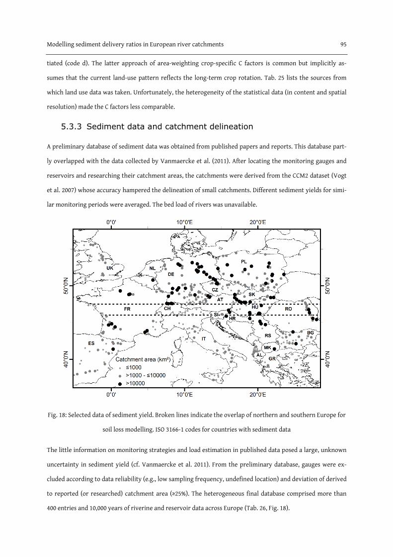
Modelling sediment delivery ratios in European river catchments 95
tiated (code d). The latter approach of area-weighting crop-specific C factors is common but implicitly as-
sumes that the current land-use pattern reflects the long-term crop rotation. Tab. 25 lists the sources from
which land use data was taken. Unfortunately, the heterogeneity of the statistical data (in content and spatial
resolution) made the C factors less comparable.
5.3.3 Sediment data and catchment delineation
A preliminary database of sediment data was obtained from published papers and reports. This database part-
ly overlapped with the data collected by Vanmaercke et al. (2011). After locating the monitoring gauges and
reservoirs and researching their catchment areas, the catchments were derived from the CCM2 dataset (Vogt
et al. 2007) whose accuracy hampered the delineation of small catchments. Different sediment yields for simi-
lar monitoring periods were averaged. The bed load of rivers was unavailable.
Fig. 18: Selected data of sediment yield. Broken lines indicate the overlap of northern and southern Europe for
soil loss modelling. ISO 3166-1 codes for countries with sediment data
The little information on monitoring strategies and load estimation in published data posed a large, unknown
uncertainty in sediment yield (cf. Vanmaercke et al. 2011). From the preliminary database, gauges were ex-
cluded according to data reliability (e.g., low sampling frequency, undefined location) and deviation of derived
to reported (or researched) catchment area (≥25%). The heterogeneous final database comprised more than
400 entries and 10,000 years of riverine and reservoir data across Europe (Tab. 26, Fig. 18).

96 Modelling sediment delivery ratios in European river catchments
Tab. 26: Data on sediment yield
Country No. of data
sets (years)
Reference
Albania 16 (362) Grazhdani (2006); Saraçi (1996)
Austria 1 (10) Zessner (pers. comm.)
Bulgaria 32 (1084) Gergov (1996); Rousseva et al. (2006b)
Croatia 1 (163) Levashova et al. (2004)
Czech Republic 25 (467) CHMÚ (2006); ICPDR (2004, 2005, 2006, 2007b, a, 2009, 2010b, a); ICPER (2005a, b, 2006,
2007, 2008, 2009, 2010); Kliment et al. (2007); Krása et al. (2005)
France 24 (222) Asselman (2000); Crouzet et al. (2004); Dumas (2007); Mano et al. (2006); Meybeck et al.
(2003); Moatar et al. (2006); Pistocchi (2008); Pont et al. (2002)
Germany 86 (2044) Asselman (2000); Bechteler (2006); Behrendt et al. (1999); ICPDR (2004, 2005, 2006, 2007b,
a, 2009, 2010b, a); ICPER (2005a, b, 2006, 2007, 2008, 2009, 2010); LfU (2009a, b); LUA (2007);
LUBW (2009); NLWKN (2011); Pistocchi (2008); Schröder and Theune (1984); Weiss (1996)
Greece 7 (112) Zarris et al. (2007)
Hungary 21 (225) Bogárdi (1957); Bogárdi et al. (1983); ICPDR (2004, 2005, 2006, 2007b, a, 2009, 2010b, a);
Jordan et al. (2005); Kovács (pers. comm.)
Italy 58 (684ab) Diodato and Grauso (2009); Grauso et al. (2008); Torri et al. (2006); van Rompaey et al.
(2005); van Rompaey et al. (2003a)
Macedonia 1 (16) Gobin et al. (2003)
Netherlands 1 (11) Ward (2008)
Poland 48 (1687) Brański and Banasik (1996); Łajczak (2003)
Romania 19 (1179) Levashova et al. (2004); Rădoane and Rădoane (2005); Rădoane et al. (2008)
Serbia 4 (499) Djorović (1992); Levashova et al. (2004)
Slovakia 8 (44) SHMÚ (2006, 2007, 2008, 2009, 2011a, b, d, c)
Slovenia 6 (83) ARSO (2005, 2006, 2007, 2008, 2009); ICPDR (2004, 2005, 2006, 2007b, a, 2009, 2010b, a);
Ulaga (2005)
Spain 29 (503ac) Batalla and Vericat (2011); Pistocchi (2008); Verstraeten et al. (2003)
Switzerland 1 (14) Asselman (2000); Pistocchi (2008)
United King-
dom
29 (265ad) Brazier (2004); Bronsdon and Naden (2000); Neal et al. (2006); Rowan et al. (1995); Small et
al. (2003); Walling et al. (2003); Wass and Leeks (1999)
a Long-term reservoir data not included, b 24 reservoirs, c 17 reservoirs, d 12 reservoirs
It consisted of average and annual data which had either been reported as “suspended-sediment yield”, “total
suspended solids”, or “sediment yield”. For total suspended solids, the low temporal resolution impeded the

Modelling sediment delivery ratios in European river catchments 97
estimation of the erosion-independent base load (e.g., industrial effluents, phytoplankton) (section 3.4.2.2).
The critical yield as the product of surface runoff and concentration of total suspended solids was available for
some gauges in southern Germany (Tab. 10, p. 51). The impact of data disaggregation on lumped SDR models
was exemplarily assessed for non-alpine gauges.
5.3.4 Modelling sediment delivery ratios (SDR)
Neither the USLE nor the PESERA model predicts SY. SDR were thus calculated as ratio of sediment yield and
soil loss (SDRcalc) to adjust the soil loss estimates. For the USLE maps, the SDR subsume both catchment and in-
stream retention. As the PESERA model estimates the net soil loss from hillslopes, PESERA-derived SDR are
more related to the in-stream retention. To evaluate the impact of algorithm and data choices and assess the
applicability of SDR models, four common empirical models of different complexity were applied to regress
SDRcalc (in %) to catchment properties (Eqs. 22–25).
Of these models, the Area model is the most widely used in erosion studies (cf. de Vente et al. 2007). The Com-
plex model was derived from chapter 3 and recent approaches applied in the Mediterranean zone (Diodato
and Grauso 2009) and Europe (Delmas et al. 2009). It reflects the influence of precipitation (Pr), land use and
land cover (Ar), topography (β), and drainage density (DD) on sediment connectivity and transport in river
catchments. Pr is the long-term average annual precipitation (in mm∙yr-1) and Ar the fraction of arable land
(%). The average slope β (in °) is related to other common topographic parameters such as the fraction of flat
areas (Delmas et al. 2009). DD (km∙km-2) is the ratio of stream length (in km) to catchment area A (in km²) and
is related to the transport distance of sediments and the fraction of the catchment effectively connected to
streams (Delmas et al. 2009). ζ11–ζ41 and η1–η4 are empirical coefficients.
The CLC classes 21–24 and 211–244 (except 23 and 231) and the GlobCover classes 11–20 were counted as arable
land. The input data for Pr in the Complex model was identical to the R factor, i.e. Pr was either derived from
the CCM2 or the GPCC dataset (section 5.3.2.1). The stream length was taken from the CCM2 data.
Complex model 14ζ13ζ12ζ11ζ1 ArPrDDβηSDR ⋅⋅⋅⋅= Eq. 22
Slope-arable model ( ) 22ζ21ζ2 20ArβηSDR +⋅⋅= Venohr et al. (2011) Eq. 23
Slope model 31ζ3 βηSDR ⋅= e.g., Diodato and Grauso (2009) Eq. 24
Area model 41ζ4 AηSDR ⋅= e.g., de Vente et al. (2007) Eq. 25

98 Modelling sediment delivery ratios in European river catchments
5.3.5 Statistical analyses
The consequences of algorithm and data choice were assessed for the i) soil loss, ii) SDR and iii) SY as product
of SDR and soil loss. Ratios and correlation coefficients were calculated between alternative maps to quantify
quantitative and qualitative impacts. Kendall’s τ was used as correlation coefficient because the data was not
normally distributed. High τ values indicate a low impact on SDR and SY models because of spatial similarity.
For SDR and SY, the regression models were evaluated with the Nash-Sutcliffe model efficiency (ME) and ad-
justed r². ME range from −∞ to 1 with higher values corresponding to more accurate and more suitable models.
If ME>0, the variance of model residuals is lower than the variance of observed data. The model sensitivity was
assessed as change in ME and r². The more noticeable the change, the higher the model sensitivity is. Given
the different distribution of SDR and SY, deviating SDR did not necessarily made the modelled SY fit the ob-
served values. SY were thus adjusted with a linear regression model (y=a1x+a0) prior the analyses. The model
uncertainty in USLE results and modelled SY was calculated as ratio of the maximum and minimum value.
Tab. 27: Ad-hoc criteria to exclude gauges and catchments from regression analyses
Criteria Threshold Explanation
Fraction of arable land <10% USLE not explaining important soil erosion processes and
sediment sources (channel erosion, glacier erosion, mass
movements), low soil loss and high SY led to very high SDR
(i.e. leverage values)
Annual sediment yield >700 Mg∙km-2
Fraction of open area and
maximum elevation
>5% and >1,500 m
SDRcalc ≥10,000%
Data age ≥30 years Sediment data not reflecting current soil loss
Monitoring period <5 years Average SY not representative for long-term conditions
PESERA coverage <75% Modelled soil loss not representative
The heterogeneous sediment database consisted of catchments of different sediment yield, environmental
settings, and sediment sources as well as monitoring periods and data age. Ad-hoc criteria were defined to
reduce inconsistencies between SY and USLE as well as PESERA estimates (Tab. 27). Catchments where pro-
cesses outside the scope of both models are very likely and unreliable sediment data were excluded. The ex-
clusion criteria and their thresholds were refined evaluating the residuals and outliers during the regression
analyses. Common large residuals and influential values mark constraints of the empirical modelling frame-
work and its evaluation. As they can also mask differences between the model realisations, such values were
excluded from the statistical analyses while maintaining the sample size as large as possible. As the PESERA

Modelling sediment delivery ratios in European river catchments 99
map was not everywhere available, catchments with an overlap below 75% were considered as insufficient for
the statistical analyses. However, they were used to compare USLE alternatives.
Tab. 28: Ad-hoc definition of (sub-)regions. Catchments associated to the country their gauge falls in
Region Sub-regions Countries
North (n=149) DE (n=52) Germany
PL (n=47) Poland
W (n=19) France, western Germany, Netherlands, United Kingdom
- Austria, Croatia, Czech Republic, Hungary, Macedonia, Serbia, Slovakia,
Switzerland
Central-South East (CSE,
n=30)
- Austria, Croatia, Czech Republic, Hungary, Macedonia, Romania, Serbia,
Slovakia, Slovenia, Switzerland
South (n=95) SW (n=25) France, Spain
SE (n=47) Albania, Bulgaria, Greece, Hungary, Romania
IT (n=23) Italy
- Croatia, Macedonia, Serbia, Slovenia
Taking the remaining unexplained variability into account, the model quality and its sensitivity to the soil loss
estimation was also evaluated in several regions (Tab. 28). How do the SDR models perform in different parts
of Europe? For which soil loss map are the results acceptable (ME>0)? Are the applicability and constraints of
the empirical modelling framework and the sensitivity of ME and r² to the soil loss and SDR models con-
sistent? To answer these questions, the gauges were grouped by country and associated to the regions North,
South, and, as transition region, Central-South East (CSE). In general, the northern part of Europe (i.e. north of
the Alps) is characterised by low to moderate SY in flat and high SY in alpine areas. The climate is humid with
equally-distributed annual rainfalls. In southern Europe (mainly the Mediterranean zone), SY are higher and
the climate features a pronounced seasonality with dry summers and wet winters. Gully erosion, not covered
in the USLE and PESERA, can be an important sediment source (Vanmaercke et al. 2012a). The large regions
North and South were exemplary sub-divided.
5.4 Results and discussion
5.4.1 Soil loss maps
The soil loss estimates and model uncertainty varied widely between European regions (Figs. 19–20). Both are
not related. For the three regions in Fig. 20, the methods for estimating C and K factors influenced the USLE

100 Modelling sediment delivery ratios in European river catchments
results the most. Their average uncertainty was 60%, unlike the low uncertainty of the R factor (<10%). The
average maximum model uncertainty (of all USLE factors) was >100% with values ranging from 0% to >1,000%.
Unlike the USLE, the PESERA results were similar or, in southern Europe, even below SY. These findings are in
accordance to Vanmaercke et al. (2012a).
Fig. 19: Sediment yield and uncertainty in USLE estimates. Top: sub-regions DE, PL, and W of region North,
bottom: region CSE, sub-regions SE and SW of region South
Fig. 20: Soil loss and sediment yield for catchments in European regions (Tab. 27). PES is the PESERA map, 4-
letter codes for USLE maps (Tab. 21), SY is the sediment yield

Modelling sediment delivery ratios in European river catchments 101
Consequently, choosing the soil loss model and approximation approaches for model parameters caused not
only an enormous uncertainty in absolute values of SDRcalc but, more important for analysing the sensitivity of
SDR models, also affected the spatial pattern of SDRcalc. The correlation between all USLE maps and the PESERA
map was loose. Kendall’s τ ranged from -0.3 to 0.1 for the regions in Fig. 20 and from 0.0 to 0.25 for the whole
dataset. The correlation coefficients were significantly higher among the USLE maps with τ being maximal
between opposite R and C factors (τ>0.8). For the K and L factors, the algorithm choice affected the spatial
pattern of the soil loss, and thus SDR, more strongly. For contrasting USLE maps, the average correlation coef-
ficient τ was about 0.6 (0.45–0.72) for the complete dataset and varied from 0.36 to 0.82 among the regions.
Fig. 21: Quality and sensitivity of the Complex model in region North. Model predictions with the USLE map
2kbc (left), model sensitivity to soil loss estimation (right, 2kbc marked with an asterisk), PES is the PESERA
map, alphanumeric characters refer to the alternative USLE factors (Tab. 21)
5.4.2 Sediment delivery ratio (SDR)
The SDR models were insufficient to explain the spatial variability of SDR of the pre-selected river catchments
(Fig. 21). Despite the ad-hoc criteria, influential values strongly affected the regression analyses. High SDRcalc
and residuals were found to be associated to the criteria defined in Tab. 27. They point to sediment sources
not considered in the soil loss models and are discussed as model and data limitations in the (sub-) regions.
5.4.2.1 Region North
5.4.2.1.1 Sub-region DE
The Complex model (Eq. 22) well explained the SDR variability with some USLE maps (Tab. 29). While the
Slope-arable model (Eq. 23) was also, albeit to a lesser degree, acceptable, the Slope and Area models (Eqs. 24–
25) could not adequately describe the spatial pattern at all. The Complex and Slope-arable models were sensi-
tive to the approximation of the K factor and (for USLE maps) the SDR parameterisation. The C and L factors
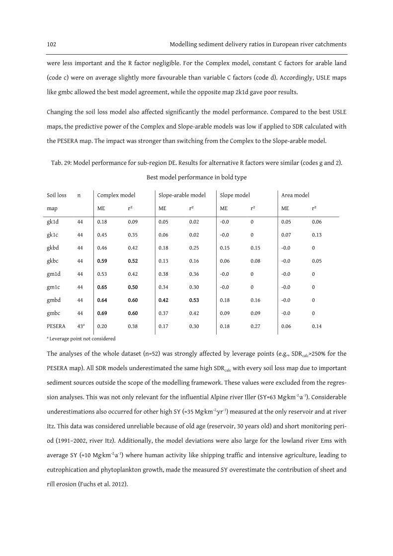
102 Modelling sediment delivery ratios in European river catchments
were less important and the R factor negligible. For the Complex model, constant C factors for arable land
(code c) were on average slightly more favourable than variable C factors (code d). Accordingly, USLE maps
like gmbc allowed the best model agreement, while the opposite map 2k1d gave poor results.
Changing the soil loss model also affected significantly the model performance. Compared to the best USLE
maps, the predictive power of the Complex and Slope-arable models was low if applied to SDR calculated with
the PESERA map. The impact was stronger than switching from the Complex to the Slope-arable model.
Tab. 29: Model performance for sub-region DE. Results for alternative R factors were similar (codes g and 2).
Best model performance in bold type
Soil loss
map
n Complex model Slope-arable model Slope model Area model
ME r² ME r² ME r² ME r²
gk1d 44 0.18 0.09 0.05 0.02 -0.0 0 0.05 0.06
gk1c 44 0.45 0.35 0.06 0.02 -0.0 0 0.07 0.13
gkbd 44 0.46 0.42 0.18 0.25 0.15 0.15 -0.0 0
gkbc 44 0.59 0.52 0.13 0.16 0.06 0.08 -0.0 0.05
gm1d 44 0.53 0.42 0.38 0.36 -0.0 0 -0.0 0
gm1c 44 0.65 0.50 0.34 0.30 -0.0 0 -0.0 0
gmbd 44 0.64 0.60 0.42 0.53 0.18 0.16 -0.0 0
gmbc 44 0.69 0.60 0.37 0.42 0.09 0.09 -0.0 0
PESERA 43a 0.20 0.38 0.17 0.30 0.18 0.27 0.06 0.14
a Leverage point not considered
The analyses of the whole dataset (n=52) was strongly affected by leverage points (e.g., SDRcalc>250% for the
PESERA map). All SDR models underestimated the same high SDRcalc with every soil loss map due to important
sediment sources outside the scope of the modelling framework. These values were excluded from the regres-
sion analyses. This was not only relevant for the influential Alpine river Iller (SY=63 Mg∙km-2∙a-1). Considerable
underestimations also occurred for other high SY (≈35 Mg∙km-2∙yr-1) measured at the only reservoir and at river
Itz. This data was considered unreliable because of old age (reservoir, 30 years old) and short monitoring peri-
od (1991–2002, river Itz). Additionally, the model deviations were also large for the lowland river Ems with
average SY (≈10 Mg∙km-2∙a-1) where human activity like shipping traffic and intensive agriculture, leading to
eutrophication and phytoplankton growth, made the measured SY overestimate the contribution of sheet and
rill erosion (Fuchs et al. 2012).

Modelling sediment delivery ratios in European river catchments 103
5.4.2.1.2 Sub-region PL
In contrast to sub-region DE, the slope-based SDR models equally well explained the spatial variability of SDR
(Tab. 30). The applicability of the SDR models was most sensitive to the L factor and the soil loss model. Satis-
factory results were obtained with the empirical L factor (code b) but not with constant erosive-slope lengths
(code 1). Model results were much better with the PESERA map than with any USLE map. Other USLE factors
and especially the parameterisation of the SDR model were less important.
Tab. 30: Model performance for sub-region PL. Results for alternative R factors were similar (codes g and 2).
Best model performance in bold type
Soil loss
map
n Complex model Slope-arable model Slope model Area model
ME r² ME r² ME r² ME r²
gk1d 29 0.16 0.09 0.09 0.13 0.10 0.15 -0.0 0
gk1c 29 0.26 0.15 0.14 0.17 0.14 0.19 -0.0 0
gkbd 29 0.49 0.44 0.46 0.46 0.48 0.47 -0.0 0
gkbc 29 0.56 0.47 0.49 0.48 0.50 0.50 -0.0 0
gm1d 29 0.06 0.17 0.05 0.17 0.04 0.11 -0.0 0
gm1c 29 0.12 0.18 0.10 0.18 0.10 0.14 -0.0 0
gmbd 29 0.36 0.38 0.40 0.36 0.39 0.30 -0.0 0
gmbc 29 0.42 0.38 0.45 0.37 0.43 0.32 -0.0 0
PESERA 27a 0.80 0.81 0.79 0.82 0.79 0.83 -0.1 0
a Two catchments outside PESERA map
The residuals were large for catchments with high SY and SDR due to model constraints. Similar to DE, the
highest values (SY>70 Mg∙km-2∙a-1) occurred in the mountainous southern Poland where landslides and channel
incision are important sediment sources (Lach and Wyżga 2002; Rejman and Rodzik 2006). Additionally, the
abundant heavy industry and mining activity in the Upper Silesian Coal Basin caused high loads of anthropo-
genic suspended matter in the lowland river Przemsza (Helios Rybicka 1996; Dulias 2010). Consequently, and
similar to the German river Ems, there was a strong mismatch in the flat terrain (β<2°) between low modelled
SDR (ζ11, ζ21, and ζ31>0) and low soil loss rates, i.e. high SDRcalc.
5.4.2.1.3 Sub-region W
The Complex and Slope-arable models gave acceptable results with some USLE maps, while the two simpler
models failed (Tab. 31). The predictability of SDR was sensitive to the choice of the R and L factors. For the
Complex model, the soil loss model was similarly relevant. In contrast to the other sub-regions, the GPCC data

104 Modelling sediment delivery ratios in European river catchments
(code g) and constant erosive-slope lengths (code 1) were much more favourable than their alternatives. Apart
from the C factor when using the L factor code b, other choices were unimportant for the model quality.
Catchments at the rivers Lowman and the Cadière were removed prior the regression analyses because they
had sparse arable land (Ar<17%) yet maximal SY (SY≈50 Mg∙km-2∙a-1). Important natural and anthropogenic
sediment sources were not covered here by the modelling framework (cf. Fiandino and Martin 2004; Walling
and Collins 2005). The comparatively low modelled soil loss led to influential SDRcalc and partially to very high
ME and r². The model performance of the Complex model was better (0.17≤ME≤0.93) compared to simpler
models (-0.14≤ME≤0.64 for the Slope-arable model).
Tab. 31: Model performance for sub-region W. Results for R factor code g were better than for code 2. Best
model performance in bold type
Soil loss
map
n Complex model Slope-arable model Slope model Area model
ME r² ME r² ME r² ME r²
gk1d 17 0.25 0.58 0.16 0.63 -0.2 0 -0.2 0.18
gk1c 17 0.22 0.67 0.14 0.69 -0.1 0 -0.3 0.27
gkbd 17 0.13 0.56 -0.0 0.59 -0.2 0 -0.2 0.28
gkbc 17 -0.2 0.64 -0.3 0.63 -0.3 0 -0.3 0.34
gm1d 17 0.20 0.57 0.07 0.59 -0.1 0 -0.3 0.05
gm1c 17 0.23 0.68 0.12 0.65 -0.1 0 -0.4 0.13
gmbd 17 0.16 0.58 -0.0 0.58 -0.1 0 -0.3 0.11
gmbc 17 -0.0 0.67 -0.2 0.62 -0.2 0 -0.4 0.17
PESERA 17 0.09 0.21 0.12 0.32 -0.0 0.11 -0.1 0
5.4.2.1.4 Entire region
After removing the catchments which showed large residuals in the sub-regions and harmonising the exclu-
sion criteria (reservoir data, SY>40 Mg∙km-2∙a-1 and Ar<20%), the final dataset (n=107) covered 12 out of the 14
countries of region North. The model performance was only acceptable with the Complex and Slope-arable
models (0.04≤ME≤0.26). The sensitivity to single USLE factors was weak. The best results were obtained with
USLE maps based on the combination of constant C factors for arable land, empirical L factors and the MUSLE
K factor (codes c, b, and m). The impact of the soil loss model, SDR parameterisation and R factor was negligi-
ble. Similar to sub-regions DE and PL, the USLE maps 2mbc and gmbc allowed the best model predictions.

Modelling sediment delivery ratios in European river catchments 105
5.4.2.2 Region CSE and sub-region SE
Without the influential but unreliable reservoir data of old age (≥24 a) and short monitoring period (5 a), no
model could describe the SDR variability in region CSE. Strong differences occurred when only catchments
covered by the PESERA map were considered (n=19). For these, positive ME in region CSE were obtained with
the Complex but not with the simpler models (Tab. 32). The model outcome was thus most sensitive to the SDR
parameterisation. Applying the same exclusion criteria, no model was adequate to explain the SDR variability
in sub-region SE (ME<0).
Tab. 32: Model performance for region CSE. Results for R factor code 2 were slightly better than for code g.
Best model performance in bold type
Soil loss
map
n Complex model Slope-arable model Slope model Area model
ME (MEb) r² ME (MEb) r² ME (MEb) r² ME (MEb) r²
gk1d 25 -0.1 (0.35) 0.32 -0.2 (-0.4) 0.02 -0.4 (-0.4) 0 -0.4 (-0.4) 0.04
gk1c 25 -0.1 (0.42) 0.36 -0.2 (-0.4) 0.01 -0.4 (-0.4) 0 -0.4 (-0.4) 0.04
gkbd 25 -0.2 (0.33) 0.35 -0.2 (-0.3) 0.06 -0.4 (-0.3) 0 -0.4 (-0.4) 0.09
gkbc 25 -0.1 (0.40) 0.39 -0.2 (-0.3) 0.05 -0.4 (-0.3) 0 -0.4 (-0.4) 0.09
gm1d 25 -0.2 (0.37) 0.30 -0.2 (-0.3) 0.03 -0.4 (-0.4) 0 -0.4 (-0.4) 0.04
gm1c 25 -0.1 (0.45) 0.34 -0.2 (-0.3) 0.02 -0.4 (-0.4) 0 -0.4 (-0.4) 0.05
gmbd 25 -0.1 (0.47) 0.34 -0.2 (-0.3) 0.09 -0.4 (-0.3) 0.03 -0.4 (-0.4) 0.08
gmbc 25 -0.0 (0.54) 0.37 -0.1 (-0.2) 0.08 -0.4 (-0.3) 0.02 -0.4 (-0.4) 0.09
PESERA 19a (0.42) 0.57 (-0.2) 0.14 (-0.2) 0.19 (-0.4) 0.02
a 6 catchments outside PESERA map, b Harmonised dataset (n=19)
All models systematically underestimated the SDR of Romanian catchments in both regions while overesti-
mating the SDR elsewhere. These catchments belong to the Siret river basin in eastern Romania. Geology,
climate and land use in the mountainous setting favour moderate to severe soil erosion by water including
gully erosion and sediment yields which are among the highest in Romania (Ionita et al. 2006; Rădoane et al.
2008; Zaharia et al. 2011). Nonetheless, the modelled soil loss was comparatively low resulting in above-
average SDR (Tab. 33). For the Romanian catchments, the Complex model predicted the SDR well with USLE
maps based on the MUSLE K factor (code m) and the PESERA map (0.64≤ME≤0.71, 0.50≤r²≤0.65) but less so with
the alternative K factor (0.35≤ME≤0.47, 0.04≤r²≤0.38). Accordingly, the sensitivity to this factor was strongest.
The sensitivity to the SDR parameterisation was comparatively low. The Slope-arable model behaved almost
equally in terms of model performance and sensitivity. Acceptable results were also possible with the simple
SDR models in combination with codes m and 1 (Area model) and the PESERA map (Slope model).

106 Modelling sediment delivery ratios in European river catchments
Tab. 33: Mean soil erosion rates (range) of catchments in regions CSE and SE (without excluded values)
Value Romania (n=12) CSE – Romania (n=12) SE – Romania (n=27)
Minimum soil loss (USLE) (Mg∙km-2∙a-1) 244 (116–451) 516 (227–821) 597 (234–987)
Maximum soil loss (USLE) (Mg∙km-2∙a-1) 571 (390–1075) 2192 (633–4656) 1473 (512–5019)
SY (Mg∙km-2∙a-1) 228 (118–394) 51 (4.5–184) 97 (4.5–451)
Minimum SDR (%) 42 (26–64) 2.5 (0.3–8.1) 6.4 (0.6–14)
Maximum SDR (%) 108 (55–191) 9.5 (1.0–23) 17 (1.0–46)
For the non-Romanian catchments in region CSE, however, the model sensitivity to the USLE parameterisation
was weaker in comparison to the SDR parameterisation and the soil loss model. The gross overestimation of
the unusually low SDRcalc of the small Kali basin at Lake Balaton (A=82 km²) affected the model performance of
the Complex model. The range of SDRcalc of this catchment (0.1–0.2%) was also much lower than the values
reported by Jordan et al. (2005) based on a distributed erosion and sediment transport model as well as de-
tailed input data (1.2–1.4%) implying far too high soil loss estimates. In contrast, other low SDRcalc of nearby
catchments at rivers Wulka in Austria (1.5<SDRcalc<3.5%) and Zala in Hungary (0.6<SDRcalc<1.1%) were found to
be consistent with literature values (Kovacs et al. 2012). Without the Kali basin, all USLE maps allowed almost
equally well predicted SDR with the Complex model (0.5≤ME≤0.6, 0.41≤r²≤0.56). The model quality was poorer
with simpler models (ME≤0.17). For the PESERA map, switching from the Complex to the Slope-arable model
had no impact on the model applicability (ME=0.27). However, the simpler models were not suitable (ME≤0).
Different results were observed for the non-Romanian catchments in sub-region SE, after removing four ex-
treme values including the Kali basin. The high SY of the river Topolnitsa (300 Mg∙km-2∙a-1) is strongly affected
by mining (Tz. Karagiozova, pers. comm.) (cf. Bird et al. 2009). A similar discrepancy of sparse arable land
(Ar<20%), i.e. low modelled soil loss, and huge SY (390 Mg∙km-2∙a-1) occurred at the river Luda Kamchiya in
Bulgaria. Although it can be assumed that sediment sources other than sheet and rill erosion are important in
many Bulgarian catchments (Rousseva et al. 2006b), the modelled soil loss and observed SY disagreed by far
the most in these two mountainous catchments. One exceptionally low value from river Maritsa was consid-
ered as not representative. The short monitoring period (1980–89) was characterised by severe droughts and
drastically diminished sediment transport throughout Bulgaria (Tz. Karagiozova, pers. comm.).
The approximation of the K and L factors had the largest impact among the USLE factors. ME were above 0.6
(Complex and Slope-arable models) and ranged from 0.4–0.5 (Slope model) when the MUSLE K and the empiri-
cal L factor were used or between -0.1 and 0.46 otherwise. Switching to the PESERA map decreased the model

Modelling sediment delivery ratios in European river catchments 107
performance even more (ME=0.17 for the Complex, ME≤0.07 for the Slope-arable and Slope models). The SDR
parameterisation was far less relevant and negligible for the most suitable maps 2mbc, 2mbd, gmbc, and
gmbd. The Area model was not appropriate at all.
5.4.2.3 Region South
The SDR models could not explain the large variability of SDR in the region South. The model performance
was poor (ME≤0). The SDR models could only be applied successfully in sub-regions.
5.4.2.3.1 Sub-region IT
The maps gmbc and 2mbc were most appropriate to predict the SDR of Italian catchments (Tab. 34). The per-
formance of the slope-based SDR models was acceptable while the Area model failed. The model quality was
sensitive to the soil loss model and USLE factors except the R factor.
Tab. 34: Model performance for sub-region IT. Results for alternative R factors were similar (codes g and 2).
Best model performance in bold type
Soil loss
map
n Complex model Slope-arable model Slope model Area model
ME (MEb) r² ME (MEb) r² ME (MEb) r² ME (MEb) r²
gk1d 22 -0.0 (-0.0) 0 -0.0 (-0.0) 0 -0.1 (-0.1) 0.0 -0.1 (-0.1) 0
gk1c 22 -0.0 (0.02) 0 0.0 (0.04) 0.03 -0.0 (-0.1) 0.0 -0.1 (-0.1) 0
gkbd 22 0.43 (0.21) 0.27 0.41 (0.15) 0.28 0.42 (0.07) 0.27 -0.1 (-0.0) 0
gkbc 22 0.45 (0.23) 0.30 0.49 (0.21) 0.32 0.46 (0.09) 0.28 -0.1 (0.02) 0
gm1d 22 0.41 (0.40) 0.20 0.27 (0.32) 0.19 0.23 (0.02) 0.13 -0.0 (0.21) 0.1
gm1c 22 0.54 (0.48) 0.27 0.36 (0.42) 0.25 0.25 (0.05) 0.14 0.08 (0.28) 0.11
gmbd 22 0.63 (0.61) 0.44 0.51 (0.49) 0.45 0.51 (0.29) 0.40 -0.1 (0.20) 0.03
gmbc 22 0.77 (0.67) 0.50 0.65 (0.60) 0.50 0.62 (0.33) 0.42 -0.1 (0.26) 0.05
PESERA 18a (0.29) 0.27 (-0.2) 0 (-0.2) 0 (-0.2) 0
a Leverage points not considered (SDRcalc>1,300%), b Harmonized dataset (n=18)
The models could not explain the average SDRcalc of the catchment of Lago di Pontecosi with the steepest aver-
age gradient (β=18°) and the least fraction of arable land (Ar=13%). The mismatch is related to constraints of
the soil loss models, although sheet and rill erosion contribute in general only partly to the high SY of the
Italian catchments (49–650 Mg∙km-2∙a-1, median 237) (cf. de Vente et al. 2006).

108 Modelling sediment delivery ratios in European river catchments
5.4.2.3.2 Sub-region SW
In the sub-region SW, the outcome of the Complex model was acceptable while the simpler SDR models were
not adequate (with USLE maps; Tab. 35). Apart from the strong sensitivity to the SDR parameterisation, the
results were sensitive to the soil loss model and the K but not the other USLE factors. The best results were
achieved with USLE maps based on the K factor code k while its alternative was less suitable. For the Complex
model, the impact of the soil loss model was similar to the K factor. Better results were obtained with USLE
maps. In contrast, the PESERA map was much more suitable for predicting SDR with the Slope-arable model.
Tab. 35: Model performance for sub-region SW. Left: whole sub-region, right: Spanish data. Results for R factor
code 2 were slightly better than for code g. Best model performance in bold type
Soil loss
map
n Complex model Slope-arable model n Complex model Slope-arable model
ME r² ME r² ME r² ME r²
2k1d 22 0.42 0.55 -0.0 0.11 16 0.26 0.23 0.11 0.15
2k1c 22 0.46 0.65 -0.1 0.16 16 0.28 0.25 0.11 0.14
2kbd 22 0.42 0.64 0.02 0.27 16 0.17 0.17 -0.0 0.06
2kbc 22 0.47 0.73 -0.0 0.30 16 0.20 0.19 -0.0 0.05
2m1d 22 0.28 0.43 -0.0 0.11 16 0.22 0.19 0.14 0.23
2m1c 22 0.30 0.52 -0.1 0.14 16 0.23 0.20 0.14 0.22
2mbd 22 0.26 0.49 -0.0 0.21 16 0.14 0.06 0.05 0.10
2mbc 22 0.28 0.58 -0.1 0.24 16 0.15 0.07 0.05 0.09
PESERA 22 0.33 0.62 0.29 0.34 16 0.29 0.14 0.21 0.08
Besides river Cadière in southern France (section 5.4.2.1.3), the suspiciously low SY measured at the Spanish
reservoir La Tranquera were not used in the analyses. All regression models overestimated its exceptionally
low SDRcalc (1.4–2.7%). However, the observed 8 Mg∙km-2∙a-1 had been attributed to either measurement errors
or human activity in the catchment (Sanz Montero 2002). Additionally, the simple modelling framework did
not consider important sediment sources (gully and bank erosion) and controlling factors (grazing intensity,
protective land cover) of the SY pattern (de Vente et al. 2005). The mismatch of high SY and low modelled soil
loss led to the very high SDRcalc of some Spanish catchments. The underestimation of these SDR was strongest
for the reservoir Fuensanta (SY=680 Mg∙km-2∙a-1), whose mountainous catchment had the least arable land in
sub-region SW (Ar=12%). To emphasize the differences between the alternative models, this common and
influential outlier was not considered.

Modelling sediment delivery ratios in European river catchments 109
The SY of Spanish catchments (27–540 Mg∙km-2∙a-1) were measured in reservoirs and were much higher than
the French river data (SY<45 Mg∙km-2∙a-1). Despite the homogeneous measurement technique in Spain, the
predictive power of the SDR models was lower than in the region SW given the model limitations. The sensi-
tivity of the regression models to the SDR and USLE parameterisation was similar yet less pronounced.
5.4.3 Sediment yield (SY)
For analysing the sensitivity on SY, problematic and influential catchments were not considered. The SDR
models have been applied to the refined regions of the previous section. Due to the poor prediction of SDR in
most regions, the Slope and Area models are not addressed in this section.
5.4.3.1 Region North
The Complex and Slope-arable models predicted well the variability of SY in the different parts of region
North (Tab. 36). The adjustment of the modelled SY was only significant when applying the PESERA map and
the R factor code g in the sub-region W. However, the model quality and sensitivity of SY estimates to the soil
loss estimation differed not only between the regions but also between SDR and SY. In general, ME and r² were
higher and the model sensitivity lower for SY than for SDR. Furthermore, the relative impact of soil loss, SDR
parameterisation and USLE approximation differed.
The SDR models equally well explained the spatial pattern of SY in the sub-region PL. Unlike SDR, the SY pre-
diction was not sensitive to the L factor of the USLE. Accordingly, the remarkably good SDR results with the
PESERA map did not positively affect the prediction of SY. In sub-region DE, however, the model sensitivity
was more pronounced, especially for the Slope-arable model. Similar to the SDR prediction, the MUSLE K fac-
tor (code m) was more suitable than its alternative. The impact was stronger for the Slope-arable than for the
Complex model. Likewise, the sensitivity of the SDR model to the L and C factors was negligible for the Com-
plex model but not the Slope-arable model. In contrast to the SDR, the model agreement was better with vari-
able C for arable land (code d) and constant erosive-slope lengths (code 1) instead of their alternatives. How-
ever, both SDR models were most sensitive to the soil loss estimation. Using the PESERA map instead of the
USLE maps led to much lower ME, which could not be compensated by adjusting the modelled SY.
The soil loss model was also most important for the model applicability in sub-region W. Again, the results
were better with the USLE maps than with the PESERA map. ME and r² were higher with USLE maps based on
the R factor code 2 – in contrast to the SDR results. The discrepancy was especially large for the unadjusted

110 Modelling sediment delivery ratios in European river catchments
Complex model (-0.2<ME≤0.5 with code 2 and ME<0.1 with code g). Unlike the SDR, the model quality was also
sensitive to the USLE K factor. The influential deviation of one catchment was reduced with the adjustment.
Tab. 36: Modelled SY in region North. Results for R factor code 2 similar to code g for sub-regions DE and PL
and better for sub-region W. Best model performance in bold type
Soil loss map DE PL W
Complex Slope-arable Complex Slope-arable Complex Slope-arable
ME r² ME r² ME r² ME r² MEab r² ME r²
gk1d 0.57 0.56 0.53 0.52 0.77 0.76 0.73 0.72 0.61 0.58 0.62 0.60
gk1c 0.60 0.59 0.37 0.35 0.81 0.81 0.76 0.76 0.59 0.57 0.64 0.61
gkbd 0.61 0.60 0.42 0.41 0.84 0.83 0.82 0.82 0.55 0.52 0.58 0.55
gkbc 0.57 0.56 0.23 0.21 0.87 0.86 0.84 0.83 0.54 0.51 0.60 0.57
gm1d 0.75 0.74 0.71 0.70 0.70 0.69 0.75 0.74 0.51 0.47 0.51 0.48
gm1c 0.72 0.71 0.53 0.52 0.74 0.73 0.77 0.77 0.47 0.43 0.47 0.43
gmbd 0.72 0.72 0.62 0.62 0.76 0.75 0.82 0.81 0.45 0.42 0.46 0.43
gmbc 0.65 0.64 0.42 0.41 0.78 0.78 0.82 0.82 0.42 0.38 0.41 0.37
PESERA 0.19 0.17 0.13 0.11 0.77 0.77 0.69 0.76 0.32 0.28 0.28 0.24
a Offset of linear SY adjustment of SY differs significantly from 0 (p<0.05), b Only significant for R factor code g
Both SDR models also predicted sufficiently the variability of SY in the entire region North with some USLE
maps (0.2<ME≤0.42, 0.2<r²≤0.41 after adjustment). Two catchments commonly deviated: the Kali basin whose
low SY was grossly overestimated (see section 5.4.2.2) and a catchment in southern France. Even though the
residuals increased for SY above 30 Mg∙km-2∙yr-1, the large deviation of the French catchment (SY=32 Mg∙km-2)
was attributed to the short monitoring period of 5 years. Without both catchments, the model performance
improved (0.30≤ME≤0.48 after adjustment).
In accordance to the sub-regions DE and W, the PESERA map was less favourable than the USLE maps. In fact,
the model performance was most sensitive to the soil loss model followed by the R and C factors. The C factor
code c and R factor code g allowed better model results than their alternatives. Considering the prediction of
SDR and SY, no soil loss map can be considered as “most suitable” everywhere. Nonetheless, the maps 2kbc in
combination with the Complex model allowed acceptable results in all parts of region North. Compared to the
other maps, the explained variability in the entire region North was also among the highest (r²=0.37, ME=0.38).

Modelling sediment delivery ratios in European river catchments 111
5.4.3.2 Regions CSE and South
Applying the SDR models to predict the SY variability of catchments in southern Europe was of limited use
(ME<0). Satisfactory results were only possible for sub-regions (Tab. 37). In comparison to region North, the
sensitivity to the soil loss model was similar but to the SDR model more pronounced. The model quality and
explained variability dropped considerably when the PESERA instead of USLE maps was used. Moreover, ME
were negative with the PESERA map.
For the Romanian catchments in regions CSE and SE, both SDR models allowed satisfactory SY predictions
(ME=0.55-0.72 for the Complex, ME=0.45-0.64 for the Slope-arable model). The model sensitivity to USLE fac-
tors was accordingly low. The best results were achieved with the maps 2m1c and gm1c. The SDR models were
again most sensitive to the soil loss model. The results were poor with the PESERA map (ME=r²=0).
Tab. 37: Modelled SY in regions CSE, SE and SW. Results for R factor code 2 differed slightly from code g. Best
model performance in bold type
Soil loss map CSE (without Romania) SEa (without Romania) SW
Complex Slope-arable Complex Slope-arable Complex Slope-arable
ME r² ME r² ME r² ME r² ME r² ME r²
gk1d 0.77 0.74 0.30b 0.23 0.39 0.36 0.30 0.27 0.27cd 0.24 0.18c 0.14
gk1c 0.79 0.77 0.30b 0.23 0.42 0.40 0.32 0.29 0.28cd 0.24 0.14bc 0.10
gkbd 0.66 0.62 0.20b 0.12 0.53 0.52 0.45 0.42 0.43 0.40 0.26 0.23
gkbc 0.73 0.70 0.22b 0.14 0.56 0.55 0.46 0.44 0.43 0.40 0.18bdc 0.14
gm1d 0.81 0.79 0.43 0.37 0.52 0.50 0.44 0.42 0.23cd 0.19 0.16bc 0.12
gm1c 0.79 0.77 0.39 0.33 0.55 0.54 0.46 0.44 0.23cd 0.19 0.13bc 0.08
gmbd 0.75 0.73 0.36 0.29 0.62 0.60 0.54 0.52 0.25 0.22 0.17bdc 0.12
gmbc 0.79 0.77 0.36 0.30 0.64 0.63 0.56 0.54 0.25cd 0.21 0.12bc 0.08
PESERA 0.04b 0 0.05b 0 0.16bc 0.12 0.21c 0.17 0.41c 0.38 0.28c 0.24
a Without one leverage value (outside the PESERA map), b Slope of linear SY adjustment differs not significantly from 0 (p<0.05), c Offset of linear SY adjustment differs significantly from 0 (p<0.05), d Only significant for R factor code g
The results for the non-Romanian catchments in CSE and SE slightly differed. The combination of the Complex
model and USLE predicted the variability of SY in region CSE much better than alternative combinations. Alt-
hough the results were better with the MUSLE K factor (code m) instead of code k (before the adjustment), the
sensitivity was low to the USLE parameterisation compared to the SDR model. In contrast, satisfactory results
for region SE were obtained equally well with both SDR models (ME≤0.78). However, the evaluation for region

112 Modelling sediment delivery ratios in European river catchments
SE was affected by an influential value (SY=450 Mg∙km-2∙a-1). Without it, the impact of changing the SDR model
as well as the K and L factors became more distinct while ME and r² decreased (Tab. 37).
The model performance for catchments in the region SW corresponded to the SDR results. Without the linear
adjustment, the Complex model partly allowed acceptable results (ME≤0.39) while the Slope-arable model
almost failed to capture the regional SY variability (ME≤0.12). To obtain acceptable model results, the USLE
parameterisation was more important than the choice of the SDR model. In contrast to the SDR prediction and
other (sub-)regions, all ME were negative except for USLE maps based on the empirical L factor code b and the
K factor code k. For Spanish catchments, the model quality was even lower (ME<0.3). Large residuals of the
highest SY and SDR (section 5.4.2.3.2) were decisive in Spain and the region SW. The negative ME revealed that
the calibrated SDR models could not sufficiently explain the SY with the PESERA map without linear adjust-
ment. Only after the adjustment, the model performance was comparable to the USLE maps. In Italy, however,
the results only partly reflected the model performance for SDR predictions. They were best for the combina-
tion of MUSLE K (code m) and constant C factors for arable land (code c; ME≤0.28 without adjustment). The
alternative K factor code k was less appropriate. The sensitivity to the L factor and the soil loss model was low
compared to the SDR prediction. Apart for the most suitable soil loss maps (gm1c, 2m1c, PESERA), the SDR
model hardly affected the model performance.
Fig. 22: Uncertainty in modelled sediment yield and soil loss. Left: SY (left boxes) and soil loss (right boxes),
right: median values, SY calculated with Complex SDR model
The results confirmed the findings for northern Europe that the empirical SDR models were in general less
adequate to relate PESERA estimates to the observed SY. They also showed that the Complex model was more
appropriate for southern Europe than the Slope-arable model. Again, no USLE map was “best” for all regions.
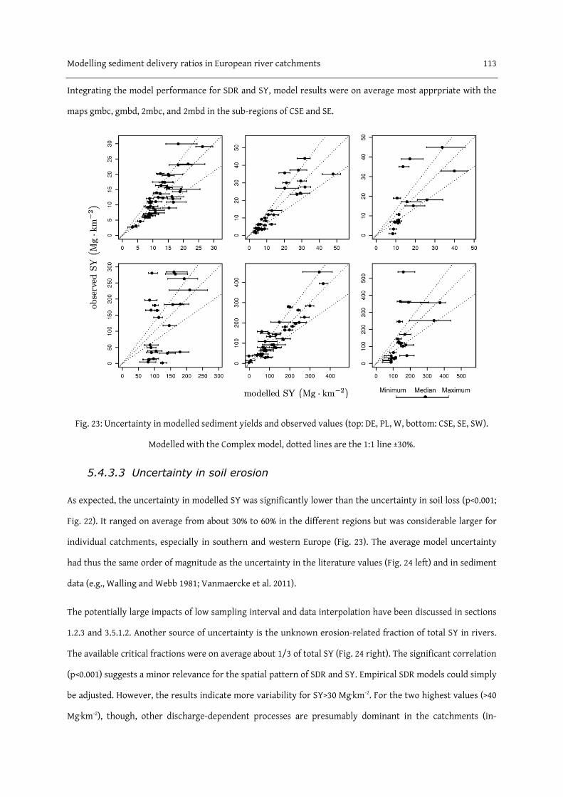
Modelling sediment delivery ratios in European river catchments 113
Integrating the model performance for SDR and SY, model results were on average most apprpriate with the
maps gmbc, gmbd, 2mbc, and 2mbd in the sub-regions of CSE and SE.
Fig. 23: Uncertainty in modelled sediment yields and observed values (top: DE, PL, W, bottom: CSE, SE, SW).
Modelled with the Complex model, dotted lines are the 1:1 line ±30%.
5.4.3.3 Uncertainty in soil erosion
As expected, the uncertainty in modelled SY was significantly lower than the uncertainty in soil loss (p<0.001;
Fig. 22). It ranged on average from about 30% to 60% in the different regions but was considerable larger for
individual catchments, especially in southern and western Europe (Fig. 23). The average model uncertainty
had thus the same order of magnitude as the uncertainty in the literature values (Fig. 24 left) and in sediment
data (e.g., Walling and Webb 1981; Vanmaercke et al. 2011).
The potentially large impacts of low sampling interval and data interpolation have been discussed in sections
1.2.3 and 3.5.1.2. Another source of uncertainty is the unknown erosion-related fraction of total SY in rivers.
The available critical fractions were on average about 1/3 of total SY (Fig. 24 right). The significant correlation
(p<0.001) suggests a minor relevance for the spatial pattern of SDR and SY. Empirical SDR models could simply
be adjusted. However, the results indicate more variability for SY>30 Mg∙km-2. For the two highest values (>40
Mg∙km-2), though, other discharge-dependent processes are presumably dominant in the catchments (in-

114 Modelling sediment delivery ratios in European river catchments
stream erosion, urban runoff) which could not be separated from sheet and rill erosion (section 3.5.2) thus
supporting the refined exclusion criteria for region DE and North.
Fig. 24: Uncertainty in sediment data. Left: Variability of reported sediment yields, ratios of values from differ-
ent data sources shown if the monitoring period fell inside a longer monitoring period, monitoring periods
estimated for reservoirs in Spain (reported as “several decades”) (stars), right: Estimated sediment yield of
surface runoff (critical SY) and observed values for non-alpine catchments in southern Germany
5.5 Discussion – Application and evaluation of SDR models
The findings show that simple empirical SDR models can sufficiently explain the spatial variability of SDR and
SY of European river catchments. As expected, the soil loss and SDR models have a strong impact on the model
applicability. Among the tested alternatives, combining the USLE and the Complex model based on topogra-
phy, drainage density, land cover, and precipitation allowed the most satisfactory results. Empirical SDR mod-
els with fewer parameters are less applicable in southern Europe. Diodato and Grauso (2009), with more de-
tailed soil loss data and a few catchments, as well as Pistocchi (2008), with different sediment data and SDR
models, made similar observations. Of the three alternative SDR models, the Slope-arable model is almost
equally applicable in northern Europe while the Area and Slope models cannot be recommended. The poor
results with the PESERA map reveal that the fundamentally different concept behind PESERA requires other
catchment features to link its outcomes to observed sediment yields.
Besides highly uncertain soil loss and significantly less yet considerably uncertain modelled SY, the uncertain-
ty in approximating USLE factors for European soil loss maps also affects the performance of SDR models. In
northern Europe, the impact is stronger than the impact of changing from the Complex to the Slope-arable
model. None of the approaches can be recommended to optimally predict SDR and SY everywhere. However,

Modelling sediment delivery ratios in European river catchments 115
the map 2kbc is proposed as most suitable for predicting SY in European regions, although the K factor code k
was less favourable for predicting SDR and the sensitivity to the R factor was usually low.
The favourable approximation of USLE factors at large scales is “more suitable” rather than “more precise”
and, without doubt, the uncertainty goes far beyond two alternative approximations. The results were repeat-
edly similar or even better with constant C factors for arable land, although variable values might be consid-
ered as better conforming to the variability of soil loss in river catchments. In either case, average values (for
C factors and crops) only crudely reflect the heterogeneity of the C factor. The same holds true for the other
USLE factors. Therefore, the study can shed only some light into the uncertainty and sensitivity of SDR models
at large scales. Nonetheless, the findings clearly show that carefully choosing the approaches to estimate USLE
factors can positively affect the performance of SDR models. Therefore, conceptually new approaches to ob-
tain USLE factors like interpolating local K factors instead of using the coarse soil classes of the European Soil
Database (Panagos et al. 2012) offer not only the possibility to describe the variability of soil erodibility differ-
ently (if not better) but also to further improve the applicability of empirical SDR models.
The results also show that model quality and sensitivity differ between SDR and SY. For instance, the sensitivi-
ty to the soil loss model was much stronger when predicting SY instead of SDR. SY predictions can also be
acceptable with poorly predicted SDR, contrary to what might be expected. In addition, model uncertainty and
sensitivity are variable in space. SDR models should thus be evaluated against SY and SDR in different regions.
Furthermore, the variable impacts of algorithm and data choices on model quality and sensitivity support the
hypothesis that regional findings cannot be simply extrapolated.
Despite the uncertainty in model parameterisation, the replacement of USLE maps to obtain more satisfactori-
ly applicable SDR models is limited. In the present study, none of the evaluated algorithm and data choices
overcomes some general mismatches between the modelling framework and the sediment yield as integral of
all sediment sources. For instance, high soil erosion rates occurring in Mediterranean catchments prone to
gully erosion (García-Ruiz 2010; Cantón et al. 2011) are only marginally related to USLE and PESERA estimates.
In agreement to previous studies (van Rompaey et al. 2003b), only very narrow solutions for SDR models can
be expected. Other catchment features like the abundance of gullies and landslides have been shown to be
better predictors for the high SY in countries like Italy and Spain (de Vente et al. 2005; de Vente et al. 2006).
Other plausible reasons for influential model deviations in all parts of Europe require more specific knowledge
about river catchments. This covers natural processes in areas with sparse arable land (Ar≤20%) like bank and
moorland erosion and anthropogenic factors like mining, water diversion and sediment trapping in reservoirs.
116 Modelling sediment delivery ratios in European river catchments
The huge uncertainty in the heterogeneous sediment data (Vanmaercke et al. 2011) has an unknown effect on
the applicability, uncertainty and sensitivity of SDR models. Important sources are related to the temporal
variability of soil loss and sediment transport. For instance, SY are more uncertain and less representative for
long-term average conditions if measured over short monitoring periods (Vanmaercke et al. 2012b). The SY of
different age also vary considerably (Fig. 24 left) and are less comparable. Information on the monitoring pe-
riod (and thus data age) is often readily available and should be used to qualitatively assess the reliability and
comparability of sediment data. However, other vital information about sampling frequency and data interpo-
lation are rarely provided.
The topic of data comparability also comprises how SY are measured (e.g., in suspension, as sedimentation
rate). In the present study, data was measured as either “suspended solids” or “suspended sediments” with
very few exceptions. Although using total suspended solids arguably overestimates the contribution of soil
erosion to SY, the significant correlation between erosion-related and total suspended solids in southern Ger-
many suggests that SDR models could simply be adjusted to erosion-related yields in regional studies but more
detailed data is needed for verification. In contrast, the SDR of reservoirs did not fit the SDR of river catch-
ments. The few reservoir data was usually very high and old compared to riverine data. However, the poor
model performance in both SW Europe (riverine and reservoir data) and Spain (only reservoir data) has been
primarily the consequence of limited soil loss estimates rather than incommensurable sediment data. Similar-
ly, the repeatedly large residuals of small catchments of Hungarian reservoirs might equally be explained by
the data age, the measurement technique, (ephemeral) gullies as important sediment sources (Podmanicky et
al. 2011), or by the combination of the three.
In fact, in many catchments several model and data constraints are likely to superimpose making it difficult to
pinpoint the reason for influential values and residuals. For instance in the UK (sub-region W), the USLE maps
were derived with empirical R factors from Central Europe leading to a potential overestimation of R factors
due to the high annual rainfall. Most data has also been sampled during the national Land-Ocean Interaction
Study (LOIS) programme during the 1990s. Therefore, the sediment yield is probably not representative for
long-term average conditions. Additionally, the sediment yield of catchments in flat terrain with sparse arable
land ranges from below to above average (1–60 Mg∙km-2∙a-1). While low SY are in agreement with low USLE S
and C factors, the high SY suggest other important sources of (suspended) sediments (e.g., Walling et al. 2002).
The broad range of natural and artificial conditions and the unknown uncertainty in the heterogeneous sedi-
ment data hamper the calibration and evaluation of any large-scale erosion model. Sediment budgets of

Modelling sediment delivery ratios in European river catchments 117
catchments and techniques like source fingerprinting and un-mixing models are already used to break up the
black box “sediment yield” (Walling et al. 2011; Hinderer 2012). A sufficient number of such sediment budgets
across Europe would certainly be helpful to overcome some problems of calibrating and assessing empirical
SDR models in the future.
5.6 Conclusions
The many approximations of USLE factors used in the past in large-scale studies, the different (potential) soil
loss maps make the uncertainty in pan-European soil loss estimates large and, moreover, highly variable. Ad-
ditionally, new input data and erosion-related maps are constantly prepared. The resultant uncertain spatial
pattern of calculated sediment delivery ratios (SDR) raises the question how the application and evaluation of
empirical erosion models are affected. The empirical model character and the limited input data do not allow
judging any alternative model realisation to be more precise in describing the soil erosion in river catchments.
The intention of this study can only be to quantify the model uncertainty and sensitivity to model, algorithm
and data choices and assess the suitability of potential soil loss maps for a specific task, namely for predicting
SDR and sediment yields of European river catchments.
Unsurprisingly, the model concept for soil loss is found to generally exert a strong impact on the performance
of SDR models. In contrast to USLE maps, the different SDR models do not fit the concept of the process-
oriented PESERA model. Other explaining factors are required to link sediment yields to PESERA estimates. In
accordance to previous studies, SDR models with more parameters are found to be more favourable to predict
the SDR and SY of European catchments. The model performance was (much) better with drainage density,
topography, precipitation and land use as model parameters than with fewer parameters such as catchment
area, topography, or a combination of topography and land use. Nonetheless, the quality of a given SDR model
and the explained variability of SDR and sediment yield are also sensitive to the approximation of USLE fac-
tors. The sensitivity varies among different regions and is in the same order of magnitude as the SDR parame-
terisation. Among the tested alternatives, the K factor (soil erodibility) is generally most important, followed
by the C and L factors (land cover, erosive-slope length). The tested different input data for the R factor (rain-
fall) is mostly less relevant. However, no soil loss map can be unanimously recommended as “the best” map
for predicting SDR and sediment yields with empirical SDR models.
Besides the sensitivity of the model performance, algorithm choices are also a significant source of uncertain-
ty in modelled sediment yield. Calibrated SDR models thus require a minute documentation of the underlying
soil loss map to avoid misapplications. The model uncertainty is similar to the variability of sediment yields in

118 Modelling sediment delivery ratios in European river catchments
the literature and is arguably comparable to the uncertainty in observed sediment data and the unknown base
load of total suspended solids. For the latter, further studies are needed to verify the significant correlation
between total and critical yields observed in southern Germany.
However, all model realisations fail for the huge variability of SDR and sediment yield across Europe. Data and
model constraints only allow satisfactory regional models. Large residuals usually occur if sediment data is
unreliable and not comparable to other data and if the soil loss models do not capture important erosion pro-
cesses and sediment sources. Such data and catchments have to be removed to avoid negative impacts of out-
liers and influential residuals on the sensitivity analyses. However, the range of erosion processes, human
activity, and environmental conditions make it difficult to link modelled soil loss to literature values of sedi-
ment yield. The simple model concept, error-prone input data and the heterogeneous sediment data blur the
distinction between model errors and inappropriate sediment data.
Although additional information on sediment processes outside the scope of the USLE and PESERA models,
new approaches to better reproduce the variability of USLE factors, more parameters in the SDR model to
cover (artificial) sediment trapping, and homogeneous sediment data to reduce inconsistencies are needful to
overcome limitations in model applications, algorithm choices are expected to remain influential for the per-
formance of SDR models. Carefully choosing the soil loss map contributes to the successful application of SDR
models at large scales. For the sensitivity analyses, however, well-distributed and representative data is
strongly recommended as local findings are not valid for whole countries or river basins.

6 Summary

120 Summary
Modelling the variability of soil erosion in space and time is an important part of assessing mass transfers in
river catchments and coupling the fluxes of nutrients and contaminants with in-stream processes. The com-
plexity of the phenomenon “soil erosion” promoted the development of many models in the past. Choosing a
model depends on its purpose and data availability among other criteria. At large scales like nations and river
basins, empirical models are used to predict the spatial and temporal variability of soil loss, sediment delivery
ratios (SDR) and sediment yield from limited input data. It is good practice in any modelling – apart from
striving for better predictions – to evaluate the uncertainty of model outcomes, sensitivities to input data and
algorithms, and to identify model limitations. This dissertation thesis addresses all four topics for empirical
models in four studies in the European context because two extensive literature reviews confirmed the use of
various data and algorithms in Europe to derive erosion-related model parameters and the high variations of
sediment yield. For the first time, algorithm and data choices in modelling soil erosion at regional and Euro-
pean scales are broadly and systematically analysed. The major findings provide new insights into the rele-
vance of choices for (critical) sediment yield, topography, and soil loss – fundamental for any modelling and
evaluation of soil erosion –, into the application and evaluation of empirical soil erosion models as well as
their improved yet limited applicability at large scales.
First, data and algorithm choices for topographic parameters and critical yields of suspended solids are found
to exert significant uncertainties in the parameterisation of erosion models and in calibration and validation
data (chapters 2 and 3). The raster resolution of digital elevation models (DEM) is most influential. Especially
for coarse DEM, algorithm choices are also important even for basic parameters like the slope angle. The com-
bined effect of uncertainty in approximated factors of the universal soil loss equation (USLE) makes the uncer-
tainty in European soil loss maps and, subsequently, in modelled sediment yields even larger (chapter 5). The
findings show model uncertainties to be in the same order of magnitude as the uncertainty in measured sedi-
ment yields. A minute documentation of calibrated models is thus required to avoid misapplications.
Second, the sensitivity of models to topographic uncertainty is nonetheless low (chapters 2 and 3). Therefore,
more detailed DEM cannot improve explaining the regional variability of soil erosion in river catchments.
These results extend and generalize findings of Pan and King (2011) as well as Yong et al. (2009). In contrast,
artefacts can hamper the higher data resolution (chapter 2; de Vente et al. (2009)). As long as the DEM resolu-
tion is insufficient for GIS-based algorithms, local regression models to predict slope-length (L) factors of the
USLE are recommended (chapter 3). Unlike topography, the estimation of USLE factors and soil loss signifi-
cantly influences the model performance (chapter 5). Most important for USLE maps is the soil (K) and, to a
lesser degree, the land management (C) and L factors. However, no “best” map for all regions in Europe could

Summary 121
be identified. For the estimation of critical yields, the findings are mixed. In contrast to the spatial variability
of topographic parameters, the prediction of the annual variability of critical yields of suspended solids bene-
fits from higher data resolution and the careful method choice respectively (chapter 3). The functional
streamflow disaggregation approach (FSD) with its daily time step makes the inter-annual variability of criti-
cal yields more plausible than the statistical approach based on (multi-)annual average values. However, the
spatial model performance is worse. The significant differences for average critical yields at some monitoring
gauges require further analyses.
Third, although careful algorithm choices can thus improve the performance of SDR models, they are certain-
ly not sufficient to overcome the observed model limitations. The extensive sediment database established for
this dissertation thesis clearly shows the constraints and limitations of the regional and European application
of empirical SDR models. These limitations are essentially related to the discrepancy between the processes
and sources contributing to the observed and the modelled soil erosion (chapters 3 and 5). Specifically, the
USLE restricts the prediction of sediment yields with SDR models to non-alpine catchments outside the Medi-
terranean zone. The enormous temporal variability of soil erosion not only impedes the prediction of the
extraordinarily high sediment yields during flood years in alpine catchments (chapters 3 and 4) but also the
use of unrepresentative average sediment yields (i.e. old data, short monitoring period) for model calibration
and validation (chapters 3 and 5). Without complementing the USLE and better disaggregating the sources of
sediments and suspended solids, regional sediment data has to be used to calibrate and/or evaluate regional
SDR models. However, modelling all (relevant) soil erosion sources and processes at large scales and separat-
ing the sediment from the modelled sources and processes is far from being solved.
Fourth, the combination of pan-European data, USLE and SDR models can satisfactorily predict the variability
of sediment yields in space and time – despite the uncertainty and within the limitations mentioned above
(chapters 3–5). Nonetheless, two model improvements are proposed. Chapters 3 and 4 show that surface run-
off estimated with the FSD approach and seasonally weighted rainfall data are more suitable than simple an-
nual rainfall indices to explain the inter-annual variability of sediment yields. As daily data of water discharge
needed for FSD is not available everywhere, the generic, parsimonious RAMSES model evaluated in chapter 4
is suggested for large-scale applications. Additionally, chapters 3 and 5 highlight that calibrating SDR models
to sediment yields does not necessarily lead to good SDR predictions and poor SDR predictions do not, in turn,
mean poor predictions of sediment yield. SDR models should therefore always be calibrated and evaluated
against both SDR and sediment yields. Doing so for catchments in southern Germany, it is found that existing
SDR models without hydrological parameters cannot explain the spatial variability of SDR, despite satisfactory

122 Summary
results for sediment yields (chapter 3). Considering hydrology as a new parameter in SDR models is helpful to
significantly improve the model quality. In chapter 5, the 4-parameter SDR model derived from chapter 3 (Eq.
22) is successfully applied in different parts of Europe. Its predictions of SDR and sediment yields are generally
superior to SDR models with fewer parameters (including the one used in the MONERIS model), especially
outside Central Europe. However, even with various soil loss maps, no empirical SDR model is capable of ex-
plaining the enormous variability of SDR and sediment yields in Europe. This result is in agreement to former
studies (e.g., Verstraeten et al. 2003; de Vente et al. 2007). Reliable sediment data, regionally optimised USLE
factors, and recognizing non-USLE sediment sources are expected to improve future applications.
The extensive analysis in chapter 5 proposes a new USLE map for predicting sediment yields of European river
catchments. Based on this map (code 2kbc in chapter 5), a new 4-parameter SDR model is derived, valid for
catchments north of the Alps where USLE processes are in general the major contributors to sediment yields.
Although it is less suitable for explaining the variability of SDR, Eq. 26 satisfactorily predicts the sediment
yield of catchments with more than about 20% arable land. For sub-regions, however, specific regression mod-
els are recommended. With the on-going research to improve large-scale soil loss maps (Cerdan et al. 2010;
Meusburger et al. 2012; Panagos et al. 2012), Eq. 26 should be regularly re-evaluated. For the Mediterranean
zone, however, the combination of USLE and SDR models is of limited use due to the poor model performance
for catchments with very high SDR values. One reason is that the USLE does not consider gully erosion which
is an important sediment source in less vegetated areas (e.g., Martín-Fernández and Martínez-Núñez 2011).
245.1244.1953.0498.0 ArPrDDβ4776.0SDR −− ⋅⋅⋅⋅=
Eq. 26
285.4ESDR780.0SY +⋅⋅=
Eq. 26 predicts the long-term SDR and sediment yield (SY) from common catchment properties such as topog-
raphy (β), drainage density (DD), average annual rainfall (Pr), and land use (Ar). However, two related prob-
lems have to be kept in mind when using Eq. 26 (and any other SDR model). First, the SDR values for establish-
ing Eq. 26 are derived from total sediment yields of river catchment. This empirical model thus does not
describe the sediment flux into rivers. Second, the soil loss, sediment delivery (ratio), and in-stream sediment
retention cannot be independently validated with one sediment yield measured at the outlet. Without addi-
tional data, any model evaluation is restricted to how well the variability of SDR and sediment yield is ex-
plained and how suitable soil loss maps for this task are. Promising steps to overcome model limitations and to
(further) improve model predictions are discussed in the last chapter.

7 Outlook

124 Outlook
Some research topics can be immediately derived from the previous chapter in order to improve empirical
estimations of the variability of soil erosion in river catchments and broaden the evaluation of model uncer-
tainties and sensitivities. They comprise both the estimation of the critical fraction of total suspended solids
as well as model parameters (Tab. 38). Given the huge variability of environmental settings, soil losses, sedi-
ment yields, and SDR in Europe, an inter-regional focus is recommended.
Tab. 38: Overview of proposed further research topics
Research area Topics
Temporal variability
(RAMSES model, Eq. 13)
Generalisation of the seasonal weighting and application in non-alpine catchments
Explanatory variables for sediment yields during flood years (in different climate zones)
Disaggregation of
suspended-solid data
Critical yields of suspended solids in different parts of Europe (re-calibrating SDR models)
Assessing the separation of overland flow
Functional disaggregation of suspended-solids data
Spatial variability Regional regression models for the USLE R factor (e.g. in NW Europe)
Evaluating the relevance of measured K factors (Panagos et al. 2012) for SDR models
Matching soil loss estimations, erosion processes, and sediment yields
Disaggregation of SDR Separating in-stream and catchment retention
First, neither simple regression models nor the RAMSES approach explained the extraordinary high sediment
yields occurring during a few flood years. As most of the sediment transport is mobilised during hours to a few
days, aggregated rainfall totals are likely to mask this variability. Pan-European data of higher temporal reso-
lution like the E-OBS dataset on daily rainfall (Haylock et al. 2008) promises to be a starting point not only for
a better estimation of USLE R factors (cf. Angulo-Martínez and Beguería 2009) but also for deriving model
parameters which are closer related to the annual variability of soil erosion. At first glance, however, annual
indices based on the daily rainfall data seem not to be per se much more suitable than annual rainfall (Fig. 25).
For instance, the number of rainfall events (daily values exceeding a certain threshold) and annual percentiles
are well-correlated to annual sums. Although totals of the highest rainfalls and especially the maximum daily
rainfall deviate significantly, their variability is inconsistent for years with high soil erosion (Fig. 25c–d).
Furthermore, the huge variability of catchment responses to daily rainfall rates has also to be recognized. For
instance, if topsoils are saturated or sediment freshly deposited, subsequent rainfall is likely to trigger higher
soil erosion rates than under contrary initial conditions. Fig. 25 also shows the seasonal response which is
related to vegetation cover and, in mountainous catchments, to snowfall and melting. Therefore, further stud-
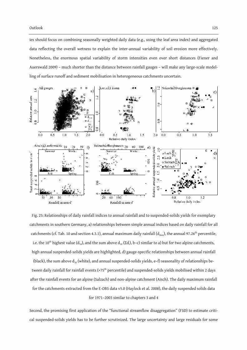
Outlook 125
ies should focus on combining seasonally weighted daily data (e.g., using the leaf area index) and aggregated
data reflecting the overall wetness to explain the inter-annual variability of soil erosion more effectively.
Nonetheless, the enormous spatial variability of storm intensities even over short distances (Fiener and
Auerswald 2009) – much shorter than the distance between rainfall gauges – will make any large-scale model-
ling of surface runoff and sediment mobilisation in heterogeneous catchments uncertain.
Fig. 25: Relationships of daily rainfall indices to annual rainfall and to suspended-solids yields for exemplary
catchments in southern Germany, a) relationships between simple annual indices based on daily rainfall for all
catchments (cf. Tab. 10 and section 4.3.1), annual maximum daily rainfall (dmax), the annual 97.26th percentile,
i.e. the 10th highest value (d10), and the sum above d10 (∑di), b–c) similar to a) but for two alpine catchments,
high annual suspended-solids yields are highlighted, d) gauge-specific relationships between annual rainfall
(black), the sum above d10 (white), and annual suspended-solids yields, e–f) seasonality of relationships be-
tween daily rainfall for rainfall events (>75th percentile) and suspended-solids yields mobilised within 2 days
after the rainfall events for an alpine (Salzach) and non-alpine catchment (Aisch). The daily maximum rainfall
for the catchments extracted from the E-OBS data v5.0 (Haylock et al. 2008), the daily suspended solids data
for 1971–2003 similar to chapters 3 and 4
Second, the promising first application of the “functional streamflow disaggregation” (FSD) to estimate criti-
cal suspended-solids yields has to be further scrutinized. The large uncertainty and large residuals for some
126 Outlook
monitoring gauges in chapter 3 call for case studies with more detailed data to test how reliably FSD separates
the “fast” mode. Additionally, the assumption in chapter 3 that this “fast” mode is always equivalent to over-
land flow needs to be further assessed. For instance, the results for the gauge at Taferlruck in chapter 3 sug-
gest that in mountainous and forested catchments not every fluctuation in water discharge is related to over-
land flow and soil erosion.
Despite the methodical development and the new software version (Carl 2011), FSD is still missing a sensitivity
analysis and the disaggregation of suspended-solids data. The latter is relevant because soil erosion events are
not only characterised by high water discharge due to overland flow but also by sediment mobilisation and
high suspended-solids concentration. Thus, approximating the critical yield as product of overland flow per
unit area (qfast in chapter 3, qf in Eq. 27) and suspended-solids concentration in overland flow (SSCf) is more
appropriate than as product of qf and the observed mixed SSC (chapter 3). Like the “shortcut” disaggregation
of total runoff q (Carl 2011), the conceptual modes of total suspended solids might be expressed as SYf(t),
SSCf(t) (fast mode), SYt(t), SSCt(t) (transient mode), SYl(t), and SSCl(t) (slow mode) where t is the time (Eq. 27).
( ) ( ) ( ) ( ) ( ) ( ) ( ) ( ) ( ) ( ) ( ) ( )tSSCtqtSSCtqtSSCtqtSSC tqtSYtSYtSYtSY llttffltf ⋅+⋅+⋅=⋅=++= Eq. 27
Third, the modelling of soil loss has to be revised to better match total or critical yields. This complex topic
not only comprises improved USLE predictions but also identifying other sediment processes. There is on-
going research on the estimation of USLE factors and soil loss in Europe (P. Panagos, pers. comm.). For in-
stance, Panagos et al. (2012) recently published a new USLE K factor map which is interpolated from measured
soil properties instead of being approximated from the coarse information stored in the European Soil Data-
base. In chapters 3 and 5, refining the regional estimation of the USLE R factor has been discussed as one step
to overcome some limitations of the evaluated SDR approaches. Meusburger et al. (2012) currently proposed a
new equation to estimate R factors in alpine areas (Switzerland). Similar efforts are needed in other regions in
Europe, especially western Europe, because the intra-annual distribution of rainfall erosivity varies among
regions and climate zones. Simply extrapolating regional approximations affects the distribution of calculated
SDR and the relationships between catchment properties and these SDR.
Unfortunately, the disaggregation techniques tested in this dissertation thesis cannot discriminate between
different soil erosion processes and sediment sources. Therefore, model adaptations should also aim at the
question of sediment sources and sediment transport. How much of the estimated gross soil loss eventually
contributes to the observed sediment yield at the catchment outlet? This in turn refers to the reliability of
USLE predictions as well as to the importance of erosion processes not described by the USLE. Although the

Outlook 127
idea of a new alpine factor in the USLE to include avalanches and other snow-related processes (Konz
Hohwieler 2010) is appealing, empirical models similar to the USLE are still not available for bank and gully
erosion. Laubel et al. (2003) found an empirical relationship between bank erosion rate and bank properties,
stream power and vegetation cover in Denmark. However, such data is not available for large-scale applica-
tions. For areas dominated by gully erosion in Spain, Martín-Fernández and Martínez-Núñez (2011) still had to
rely on USLE outcomes to approximate soil loss rates. Three approaches are feasible to better the situation: i)
evaluating sediment budgets in European river catchments, ii) evaluating the hysteresis effect during high
water discharge (e.g., Lefrançois et al. 2007), and iii) applying empirical models for sediment yields instead of
sediment delivery ratios, although findings in Spain have revealed that multiple regression models are outper-
formed by semi-quantitative factorial scoring models (Verstraeten et al. 2003; de Vente et al. 2005).
Fourth, the black box “sediment yield” (and any SDR derived from it) hides where sediments are deposited. As
erosion models for river catchments are often used as management tools, separating in-stream and catchment
retention allows better mitigating off-site effects of soil erosion (cf. Schäuble 2005; Kovacs et al. 2012). For
instance, retention in streams and on flood plains is of great ecological and economic relevance and varies
with sediment, runoff, vegetation, and stream characteristics (e.g., grain size, artificial barriers, macrophytes).
Unfortunately, sediment yields measured at the outlet are inadequate for independently validating the soil
loss as well as catchment and in-stream retention of a river catchment. The spatial disaggregation of water
discharge and sediment yield is, however, not straightforward and several disaggregation models have been
proposed in hydrology (e.g., Tarboton et al. 1998; Prairie et al. 2007). A simple approximation of net in-stream
retention is the difference between the sediment transport measured at nested monitoring gauges and reser-
voirs (Fuchs et al. 2012) – if the monitoring data is comparable and lateral fluxes are negligible. In case of un-
gauged tributaries between nested gauges, Eq. 26 can serve to close the gap in the sediment balance. For large-
scale applications, however, the in-stream retention has to be regressed to stream and catchment properties.
Finally, the input data, algorithms and model assumptions in this dissertation thesis may be critically evaluat-
ed with more detailed data in regional studies. The approaches used in chapters 3 and 5 to estimate USLE pa-
rameters have been chosen after an extensive literature review. Nonetheless, the use of pan-European data
necessarily limits the choice of appropriate algorithms and thus the evaluation of model uncertainties and
sensitivities.
For instance, USLE C factors for crops are highly variable not only among but also within countries and re-
gions. Consequently, the estimation of C factors is far more uncertain than just the difference between con-

128 Outlook
stant and crop-specific values in chapter 5. One should also be aware that the approach to use current land-
use statistics in combination with crop-specific C factors is common but nonetheless questionable because
USLE C factors are long-term means depending on crop rotation and rainfall distribution. Regression models
between recent land use and measured C factors as used in chapter 3 (Auerswald 2002) are methodologically
sound yet data demanding. They are still not available for large parts of Europe.
The estimation of the USLE L factors and delineation of water and sediment fluxes are also limited by the low
data resolution and artefacts in DEM. Several algorithms have been developed to obtain L factors from DEM
and (partly) ancillary data (as reviewed in Schäuble 1999). If high-resolution DEM and appropriate ancillary
data are available, sophisticated algorithms should be compared to those applied in the previous chapters
(e.g., Gisler et al. 2010).

References

Allan, J.D. (2004). Landscapes and riverscapes: The influence of land use on stream ecosystems. Annual Review of Ecology, Evolution, and Systematics, 35, 257–284.
Angel, J.R., Palecki, M.A. & Hollinger, S.E. (2005). Storm precipitation in the United States. Part II: Soil erosion characteristics. Journal of Applied Meteorology, 44(6), 947–959.
Angulo-Martínez, M. & Beguería, S. (2009). Estimating rainfall erosivity from daily precipitation records: A comparison among methods using data from the Ebro Basin (NE Spain). Journal of Hydrology, 379(1-2), 111–121.
Arnold, J.G., Srinivasan, R., Muttiah, R.S. & Williams, J.R. (1998). Large area hydrologic modeling and assessment Part I: Model development. JAWRA Journal of the American Water Resources Association, 34(1), 73–89.
Arnoldus, H.M.J. (1980). An approximation of the rainfall factor in the universal soil loss equation. In Boodt, M. & Gabriels, D. (Eds.), Assessment of Erosion, 127–132. Chichester: Wiley.
ARSO [Slovenian Environment Agency] (2005). Hydrološki letopis slovenije 2002 [online] [Hydrological yearbook of Slovenia]. Available from: http://www.arso.gov.si/vode/publikacije%20in%20poro%C4%8Dila/ letopisi.html.
ARSO [Slovenian Environment Agency] (2006). Hydrološki letopis slovenije 2003 [online] [Hydrological yearbook of Slovenia]. Available from: http://www.arso.gov.si/vode/publikacije%20in%20poro%C4%8Dila/ letopisi.html.
ARSO [Slovenian Environment Agency] (2007). Hydrološki letopis slovenije 2004 [online] [Hydrological yearbook of Slovenia]. Available from: http://www.arso.gov.si/vode/publikacije%20in%20poro%C4%8Dila/ letopisi.html.
ARSO [Slovenian Environment Agency] (2008). Hydrološki letopis slovenije 2005 [online] [Hydrological yearbook of Slovenia]. Available from: http://www.arso.gov.si/vode/publikacije%20in%20poro%C4%8Dila/ letopisi.html.
ARSO [Slovenian Environment Agency] (2009). Hydrološki letopis slovenije 2006 [online] [Hydrological yearbook of Slovenia]. Available from: http://www.arso.gov.si/vode/publikacije%20in%20poro%C4%8Dila/ letopisi.html.
AS [Liechtenstein Office of Statistics] (2010). Landwirtschaftsstatistik 2009 [online] [Agricultural statistics]. Available from: http://www.llv.li/amtsstellen/llv-as-publikationsarchiv/llv-as-publikationen-landwirt-schaft.htm.
Asselman, N.E.M. (2000). Fitting and interpretation of sediment rating curves. Journal of Hydrology, 234(3-4), 228–248.
Asselman, N.E.M., Middelkoop, H. & van Dijk, P.M. (2003). The impact of changes in climate and land use on soil erosion, transport and deposition of suspended sediment in the River Rhine. Hydrological Processes, 17(16), 3225–3244.
Auerswald, K. (1987). Sensitivität erosionsbestimmender Faktoren [Sensitivity of erosion determining factors]. Wasser und Boden, 39, 34–38. In German.
Auerswald, K. (1992). Predicted and measured sediment loads of large watersheds in Bavaria. 5th International Symposium on River Sedimentation, 06-10.04.1992, Karlsruhe, Vol. III, 1031–1036.
Auerswald, K. (2002). Schätzung des C-Faktors aus Fruchtartenstatistiken für Ackerflächen in Gebieten mit subkontinentalem bis subatlantischem Klima nördlich der Alpen [Estimating the C factor of the universal soil loss equation from crop statistics for sites with sub-continental to sub-atlantic climate north of the Alps]. Landnutzung und Landentwicklung, 43, 1–5. In German with English summary.
Auerswald, K. (2008). Water erosion. In Chesworth, W. (Ed.) Encyclopedia of Soil Science, 817–822. Dordrecht: Springer.

Auerswald, K. & Kainz, M. (1998). Erosionsgefährdung (C-Faktor) durch Sonderkulturen [Erosion risk (C factor) of industrial crops]. Bodenschutz, 3, 98–102. In German.
Auerswald, K. & Schwab, A. (1999). Erosionsgefährdung (C-Faktor) unterschiedlich bewirtschafteter Weinanbauflächen [Erosion risk (C factor) of different viticultural practices]. Viticultural and Enological Sciences, 54(2-3), 54–60. In German with English abstract.
Bača, P. (2008). Hysteresis effect in suspended sediment concentration in the Rybárik basin, Slovakia. Hydrological Sciences Journal, 53(1), 224–235.
Bakker, M., Govers, G., Jones, R. & Rounsevell, M. (2007). The effect of soil erosion on Europe’s crop yields. Ecosystems, 10(7), 1209–1219.
Bakker, M.M., Govers, G., van Doorn, A., Quetier, F., Chouvardas, D. & Rounsevell, M. (2008). The response of soil erosion and sediment export to land-use change in four areas of Europe: The importance of landscape pattern. Geomorphology, 98(3-4), 213–226.
Banwart, S. (2011). Save our soils. Nature, 474(7350), 151–152.
Bartolini, E., Claps, P. & D'Odorico, P. (2009). Interannual variability of winter precipitation in the European Alps: relations with the North Atlantic Oscillation. Hydrology and Earth System Sciences, 13(1), 17–25.
Bartsch, A., Gude, M. & Gurney, S.D. (2009). Quantifying sediment transport processes in periglacial mountain environments at a catchment scale using geomorphic process units. Geografiska Annaler, Series A: Physical Geography, 91A(1), 1–9.
Batalla, R.J. & Vericat, D. (2010). A review of sediment quantity issues: Examples from the River Ebro and adjacent basins (Northeastern Spain). Integrated Environmental Assessment and Management, 7(2), 256–268.
Batalla, R.J. & Vericat, D. (2011). An appraisal of the contemporary sediment yield in the Ebro Basin. Journal of Soils and Sediments, 11(6), 1070–1081.
Bauer, F. (1967). Die Stauraumverlandung in den südbayerischen Talsperren [Silting of reservoirs in the Alpine region of Bavaria]. Symposium on River Morphology, 25.9.-7.10.1967, Bern, IAHS Publication, 75, 418–429. In German with English abstract.
Bechteler, W. (2006). Sedimentquellen und Transportprozesse [Sediment sources and transport processes], ALPESERV: Sustainable sediment management of Alpine reservoirs considering ecological and economical aspects, 2. Neubiberg: Institut für Wasserwesen, Universität der Bundeswehr München. In German.
Bednorz, E. (2009). Snow cover occurrence in Central European lowlands under northern hemisphere circulation patterns. Acta Climatologica et Chorologica, 42-43, 17–28.
Behrendt, H., Huber, P., Opitz, D., Schmoll, O., Scholz, G. & Uebe, R. (1999). Nährstoffbilanzierung der Flußgebiete Deutschlands [Nutrient emissions into river basins of Germany], Texte, 75/99, FB 29625515. Berlin: German Federal Environmental Agency. In German with English abstract.
Beven, K. (1996). Equifinality and uncertainty in geomorphological modelling. In Rhoads, B.L. & Thorn, C.E. (Eds.), Scientific Nature of Geomorphology, 289–313. Chichester: Wiley.
Beven, K.J. & Brazier, R.E. (2011). Dealing with uncertainty in erosion model predictions. In Morgan, R.P.C. & Nearing, M.A. (Eds.), Handbook of Erosion Modelling, 52–79. Chichester: Wiley.
Beylich, A.A. & Sandberg, O. (2005). Geomorphic effects of the extreme rainfall event of 20-21 July, 2004 in the Latnjavagge catchment, northern Swedish Lapland. Geografiska Annaler, Series A: Physical Geography, 87A(3), 409–419.
BFS [Swiss Federal Statistical Office] (2007). Federal enterprises census 2007 (agriculture): Cultures in ares (BIO). Available from: http://www.agr.bfs.admin.ch/TableViewer/tableView.aspx?ReportId=703 [accessed 11.4.2011].
BFS, GEOSTAT & BAFU [Swiss Federal Statistical Office, Swiss Federal Office for the Environment] (1998). CORINE Land Cover 1990. Available from: http://www.bfs.admin.ch/ [accessed 1.4.2011].
Biesemans, J., van Meirvenne, M. & Gabriels, D. (2000). Extending the RUSLE with the Monte Carlo error propagation technique to predict long term average off-site sediment accumulation. Journal of Soil and Water Conservation, 55(1), 35–42.
Bilotta, G.S. & Brazier, R.E. (2008). Understanding the influence of suspended solids on water quality and aquatic biota. Water Research, 42(12), 2849–2861.
Bird, G., Brewer, P.A., Macklin, M.G., Nikolova, M., Kotsev, T., Mollov, M. & Swain, C. (2009). Dispersal of contaminant metals in the mining-affected Danube and Maritsa Drainage Basins, Bulgaria, Eastern Europe. Water, Air, and Soil Pollution, 206(1-4), 105–127.
BKG [Federal Agency for Cartography and Geodesy] (2003). Digitales Landschaftsmodell 250 [Digital landscape model 1:250,000]. Available from: http://www.bkg.bund.de.
BMU [Federal Environment Ministry of Germany] (2003). Hydrologischer Atlas von Deutschland [Hydrological atlas of Germany]. Bonn: BMU. In German.
Boardman, J. & Poesen, J. (Eds.) (2006a). Soil erosion in Europe. Chichester: Wiley.
Boardman, J. & Poesen, J. (2006b). Soil erosion in Europe: Major processes, causes and consequences. In Boardman, J. & Poesen, J. (Eds.), Soil erosion in Europe, 479–487. Chichester: Wiley.
Boellstorff, D. & Benito, G. (2005). Impacts of set-aside policy on the risk of soil erosion in central Spain. Agriculture, Ecosystems & Environment, 107(2-3), 231–243.
Bogárdi, I., Fogel, M., Duckstein, L. & Bardossy, A. (1983). Estimation of sediment loading into agricultural reservoirs with scarce data. In Plate, E. & Buras, N. (Eds.) Symposium on Scientific Procedures Applied to the Planning, Design and Management of Water Resources Systems, August 1983, Hamburg, IAHS Publication, 147, 87–98.
Bogárdi, J. (1957). Summary of the measurements made in Hungary of sediment transportation, with special reference to their quantitative bearings on erosion. Assemblée générale on Land Erosion, Instruments, Precipitations, 3-14.9.1957, Toronto, IAHS Publication, 43, Vol. 1, 277–285.
Böhm, O. & Wetzel, K.-F. (2006). Flood history of the Danube tributaries Lech and Isar in the Alpine foreland of Germany. Hydrological Sciences Journal, 51(5), 784–798.
Boix-Fayos, C., Martínez-Mena, M., Arnau-Rosalén, E., Calvo-Cases, A., Castillo, V. & Albaladejo, J. (2006). Measuring soil erosion by field plots: Understanding the sources of variation. Earth-Science Reviews, 78(3-4), 267–285.
Brański, J. & Banasik, K. (1996). Sediment yields and denudation rates in Poland. In Walling, D.E. & Webb, B.W. (Eds.) Symposium on Erosion and Sediment Yield: Global and Regional Perspectives, July 1996, Exeter, IAHS Publication, 236, 133–138.
Brardinoni, F., Hassan, M.A., Rollerson, T. & Maynard, D. (2009). Colluvial sediment dynamics in mountain drainage basins. Earth and Planetary Science Letters, 284(3-4), 310–319.
Brath, A., Castellarin, A. & Montanari, A. (2002). Assessing the effects of land-use changes on annual average gross erosion. Hydrology and Earth System Sciences, 6(2), 255–265.
Brazier, R.E. (2004). Quantifying soil erosion by water in the UK: a review of monitoring and modelling approaches. Progress in Physical Geography, 28(3), 340–365.
Brim Box, J. & Mossa, J. (1999). Sediment, Land Use, and Freshwater Mussels: Prospects and Problems. Journal of the North American Benthological Society, 18(1), 99–117.
Bronsdon, R.K. & Naden, P.S. (2000). Suspended sediment in the Rivers Tweed and Teviot. Science of The Total Environment, 251-252, 95–113.
Calanca, P., Roesch, A., Jasper, K. & Wild, M. (2006). Global warming and the summertime evapotranspiration regime of the Alpine region. Climatic Change, 79(1-2), 65–78.
Callow, J.N., van Niel, K.P. & Boggs, G.S. (2007). How does modifying a DEM to reflect known hydrology affect subsequent terrain analysis? Journal of Hydrology, 332(1-2), 30–39.
Caminiti, J.E. (2004). Catchment modelling - A resource manager’s perspective. Environmental Modelling & Software, 19(11), 991–997.
Cantón, Y., Solé-Benet, A., de Vente, J., Boix-Fayos, C., Calvo-Cases, A., Asensio, C. & Puigdefábregas, J. (2011). A review of runoff generation and soil erosion across scales in semiarid south-eastern Spain. Journal of Arid Environments, 75(12), 1254–1261.
Carl, P. (2009). Regularitäts-basierte funktionelle Disaggregation von Abfluß-Zeitreihen: Konzepte und Methodik, Software-Handbuch [Regularity-based functional streamflow disaggregation: Concepts and metholodogy, software manual], V1.00. Berlin. In German.
Carl, P. (2011). Regularitäts-basierte funktionelle Disaggregation von Abfluß-Zeitreihen: Konzepte und Methodik, Software-Handbuch [Regularity-based functional streamflow disaggregation: Concepts and metholodogy, software manual], V1.05. Berlin. In German.
Carl, P. & Behrendt, H. (2008). Regularity-based functional streamflow disaggregation: 1. Comprehensive foundation. Water Resources Research, 44(2), W02420.
Carl, P., Gerlinger, K., Hattermann, F.F., Krysanova, V., Schilling, C. & Behrendt, H. (2008). Regularity-based functional streamflow disaggregation: 2. Extended demonstration. Water Resources Research, 44(3), W03426. correction: 44(6), W06701
CBS [Croatian Bureau of Statistics] (2003). Agricultural Census 2003. Available from: http://www.dzs.hr/Eng/ censuses/Agriculture2003/census_agr.htm [accessed 18.05.2011].
Cebecauer, T. & Hofierka, J. (2008). The consequences of land-cover changes on soil erosion distribution in Slovakia. Geomorphology, 98(3-4), 187–198.
Centeri, C. (2002). The role of vegetation cover in the control of soil erosion on the Tihany Peninsula. Acta Botanica Hungarica, 44(3), 285–295.
Cerdan, O., Govers, G., Le Bissonnais, Y., van Oost, K., Poesen, J., Saby, N., Gobin, A., Vacca, A., Quinton, J., Auerswald, K., Klik, A., Kwaad, F.J.P.M., Raclot, D., Ionita, I., Rejman, J., Rousseva, S., Muxart, T., Roxo, M.J. & Dostál, T. (2010). Rates and spatial variations of soil erosion in Europe: A study based on erosion plot data. Geomorphology, 122(1-2), 167–177.
Cherry, K.A., Shepherd, M., Withers, P.J.A. & Mooney, S.J. (2008). Assessing the effectiveness of actions to mitigate nutrient loss from agriculture: A review of methods. Science of The Total Environment, 406(1-2), 1–23.
CHMÚ [Czech Hydrometeorological Institute] (2006). Hydrologická ročenka České Republiky 2005 [Hydrological yearbook of the Czech Republic]. Prague: CHMÚ.
Collins, A.L. & Walling, D.E. (2002). Selecting fingerprint properties for discriminating potential suspended sediment sources in river basins. Journal of Hydrology, 261(1-4), 218–244.
Collins, A.L., Walling, D.E. & Leeks, G.J.L. (1997). Source type ascription for fluvial suspended sediment based on a quantitative composite fingerprinting technique. Catena, 29(1), 1–27.
Colombo, R., Vogt, R.V., Soille, P., Paracchini, M.L. & de Jager, A. (2007). Deriving river networks and catchments at the European scale from medium resolution digital elevation data. Catena, 70(3), 296–305.
Coynel, A., Schäfer, J., Hurtrez, J.-E., Dumas, J., Etcheber, H. & Blanca, G. (2004). Sampling frequency and accuracy of SPM flux estimates in two contrasted drainage basins. Science of The Total Environment, 330(1-3), 233–247.

Creamer, R.E., Brennan, F., Fenton, O., Healy, M.G., Lalor, S.T.J., Lanigan, G.J., Regan, J.T. & Griffiths, B.S. (2010). Implications of the proposed Soil Framework Directive on agricultural systems in Atlantic Europe - A review. Soil Use and Management, 26(3), 198–211.
Croft, H., Kuhn, N.J. & Anderson, K. (2012). On the use of remote sensing techniques for monitoring spatio-temporal soil organic carbon dynamics in agricultural systems. Catena, 94, 64–74.
Crouzet, P., Le Gall, G., Meybeck, M. & Moatar, F. (2004). Assessment of riverine suspended solids loads to the EUROSION domain: Work Package 2.8 - Flows of sediment from river basins, Draft final report, ENV.G.4 (04D). Den Haag: European Commission, DG Environment.
D'Odorico, P., Yoo, J. & Over, T.M. (2001). An assessment of ENSO-induced patterns of rainfall erosivity in the southwestern United States. Journal of Climate, 14(21), 4230–4242.
Davies-Colley, R.J. & Smith, D.G. (2001). Turbidity, suspended sediment, and water clarity: A review. JAWRA Journal of the American Water Resources Association, 37(5), 1085–1101.
de Vente, J. & Poesen, J. (2005). Predicting soil erosion and sediment yield at the basin scale: Scale issues and semi-quantitative models. Earth-Science Reviews, 71(1-2), 95–125.
de Vente, J., Poesen, J., Arabkhedri, M. & Verstraeten, G. (2007). The sediment delivery problem revisited. Progress in Physical Geography, 31(2), 155–178.
de Vente, J., Poesen, J., Bazzoffi, P., van Rompaey, A. & Verstraeten, G. (2006). Predicting catchment sediment yield in Mediterranean environments: the importance of sediment sources and connectivity in Italian drainage basins. Earth Surface Processes and Landforms, 31(8), 1017–1034.
de Vente, J., Poesen, J., Govers, G. & Boix-Fayos, C. (2009). The implications of data selection for regional erosion and sediment yield modelling. Earth Surface Processes and Landforms, 34(15), 1994–2007.
de Vente, J., Poesen, J. & Verstraeten, G. (2005). The application of semi-quantitative methods and reservoir sedimentation rates for the prediction of basin sediment yield in Spain. Journal of Hydrology, 305(1-4), 63–86.
Dedkov, A. (2004). The relationship between sediment yield and drainage basin area. In Golosov, V., Belyaev, V. & Walling, D.E. (Eds.) International Symposium on Sediment Transfer Through the Fluvial System, August 2004, Moscow, IAHS Publication, 288, 197–204.
Delmas, M., Cerdan, O., Mouchel, J.-M. & Garcin, M. (2009). A method for developing a large-scale sediment yield index for European river basins. Journal of Soils and Sediments, 9(6), 613–626.
Destatis [Federal Statistical Office of Germany] (1971). Statistisches Jahrbuch für die Bundesrepublik Deutschland - 1971 [Statistical Yearbook for the Federal Republic of Germany]. Stuttgart, Mainz: Kohlhammer.
Destatis [Federal Statistical Office of Germany] (1980). Statistisches Jahrbuch 1980 für die Bundesrepublik Deutschland [Statistical Yearbook for the Federal Republic of Germany]. Stuttgart, Mainz: Kohlhammer.
Destatis [Federal Statistical Office of Germany] (1990). Statistisches Jahrbuch 1990 für die Bundesrepublik Deutschland [Statistical Yearbook for the Federal Republic of Germany]. Stuttgart: Metzler-Poeschel.
Destatis [Federal Statistical Office of Germany] (2009). Statistisches Jahrbuch 2009 für die Bundesrepublik Deutschland [Statistical Yearbook for the Federal Republic of Germany]. Wiesbaden: Federal Statistical Office.
Destatis [Federal Statistical Office of Germany] (2011a). Bodenbearbeitung, Bewässerung, Landschaftselemente - Erhebung über landwirtschaftliche Produktionsmethoden (ELPM): 2010 [Survey on agricultural production methods], Fachserie 3: Land- und Forstwirtschaft, Fischerei. Wiesbaden: Federal Statistical Office of Germany. In German.
Destatis [Federal Statistical Office of Germany] (2011b). Bodennutzung der Betriebe einschließlich Zwischenfruchtanbau - Landwirtschaftszählung / Agrarstrukturerhebung: 2010 [Land use by farms - Census of agriculture], Fachserie 3: Land- und Forstwirtschaft, Fischerei, Reihe 2.1.2. Wiesbaden: Federal Statistical Office of Germany. In German.

Dickinson, W.T. (1981). Accuracy and precision of suspended sediment loads. In Walling, D.E. & Tacconi, P. (Eds.) Symposium on Erosion and Sediment Transport Measurement, 22-26.06.1981, Florence, IAHS Publication, 133, 195–202.
DIN [German Institute for Standardization] (2005). Norm DIN 19708:2005-02, Bodenbeschaffenheit - Ermittlung der Erosionsgefährdung von Böden durch Wasser mit Hilfe der ABAG [Soil quality - Predicting soil erosion by water by means of ABAG].
Diodato, N. (2006). Modelling net erosion responses to enviroclimatic changes recorded upon multisecular timescales. Geomorphology, 80(3-4), 164–177.
Diodato, N. & Bellocchi, G. (2010). MedREM, a rainfall erosivity model for the Mediterranean region. Journal of Hydrology, 387(1-2), 119–127.
Diodato, N. & Grauso, S. (2009). An improved correlation model for sediment delivery ratio assessment. Environmental Earth Sciences, 59(1), 223–231.
Diodato, N., Verstraeten, G. & Bellocchi, G. (2012). Decadal modelling of rainfall erosivity in Belgium. Land Degradation & Development, early view.
Djorović, M. (1992). Ten years of sediment discharge measurement in the Jasenica research drainage basin, Yugoslavia. In Walling, D.E., Davies, T.R. & Hasholt, B. (Eds.) Symposium on Erosion, Debris Flows and Environment in Mountain Regions, July 1992, Chengdu, IAHS Publication, 209, 37–40.
Dotterweich, M. (2008). The history of soil erosion and fluvial deposits in small catchments of central Europe: Deciphering the long-term interaction between humans and the environment - A review. Geomorphology, 101(1-2), 192–208.
Dreibrodt, S., Lubos, C., Terhorst, B., Damm, B. & Bork, H.-R. (2010). Historical soil erosion by water in Germany: Scales and archives, chronology, research perspectives. Quaternary International, 222(1-2), 80–95.
Dulias, R. (2010). Landscape planning in areas of sand extraction in the Silesian Upland, Poland. Landscape and Urban Planning, 95(3), 91–104.
Dumas, D. (2007). The results of 10 years of daily observations of the flux of suspended matter in one of the main watercourses in the European Alps: The Isere at Grenoble (France). Comptes Rendus Geoscience, 339(13), 810–819.
Durbin, J. & Watson, G.S. (1950). Testing for serial correlation in least squares regression. I. Biometrika, 37(3-4), 409–428.
Durbin, J. & Watson, G.S. (1951). Testing for serial correlation in least squares regression. II. Biometrika, 38(1-2), 159–178.
Duvert, C., Gratiot, N., Némery, J., Burgos, A. & Navratil, O. (2011). Sub-daily variability of suspended sediment fluxes in small mountainous catchments - implications for community-based river monitoring. Hydrology and Earth System Sciences, 15(3), 703–713.
DWD [German Weather Service] (2008). GPCC Homepage [online]. Available from: http://gpcc.dwd.de [accessed 17.6.2011].
Dymond, J.R., Betts, H.D. & Schierlitz, C.S. (2010). An erosion model for evaluating regional land-use scenarios. Environmental Modelling & Software, 25(3), 289–298.
EC [European Commission] (2006). Proposal for a Directive of the European Parliament and of the Council establishing a framework for the protection of soil and amending Directive 2004/35/EC, COM(2006) 232 final, 22.9.2006, Brussels.
EC & ESBN [European Commission, European Soil Bureau Network] (2004). The European Soil Database distribution, V2.0, CD-ROM, EUR 19945 EN. Available from: http://eusoils.jrc.ec.europa.eul.

EEA [European Environment Agency] (2006). Vulnerability and adaptation to climate change in Europe, Technical report, 7/2005. Copenhagen: EEA.
EEA [European Environment Agency] (2007a). Corine land cover 2000. Available from: http://www.eea.europa.eu [accessed 21.10.2007].
EEA [European Environment Agency] (2007b). Europe’s environment: The fourth assessment. Luxembourg: Office for Official Publications of the European Communities.
EEA [European Environment Agency] (2010a). Corine Land Cover 1990 raster data, V13. Available from: http://www.eea.europa.eu/data-and-maps/data/ds_resolveuid/8b12c16a3c93eec2d6944abe42388d90 [accessed 1.4.2011].
EEA [European Environment Agency] (2010b). Corine Land Cover 2000 raster data, V13. Available from: http://www.eea.europa.eu/data-and-maps/data/ds_resolveuid/b00116e51c79865cf89a84162b8fd21e [accessed 1.4.2011].
EEA [European Environment Agency] (2010c). Corine Land Cover 2006 raster data, V13. Available from: http://www.eea.europa.eu/data-and-maps/data/ds_resolveuid/a645109f7a11d43f5d7e275d81f35c61 [accessed 1.4.2011].
Efthymiadis, D., Jones, P.D., Briffa, K.R., Auer, I., Böhm, R., Schöner, W., Frei, C. & Schmidli, J. (2006). Construction of a 10-min-gridded precipitation data set for the Greater Alpine Region for 1800–2003. Journal of Geophysical Research, 111, D01105.
Einsele, G. & Hinderer, M. (1997). Terrestrial sediment yield and the lifetimes of reservoirs, lakes, and larger basins. Geologische Rundschau, 86(2), 288–310.
Ekholm, P. & Lehtoranta, J. (2012). Does control of soil erosion inhibit aquatic eutrophication? Journal of Environmental Management, 93(1), 140–146.
Embleton-Hamann, C. (2007). Geomorphology for the future. In Kellerer-Pirklbauer, A., Keiler, M., Embleton-Hamann, C. & Stötter, J. (Eds.) Geomorphology for the Future. Joint meeting of the Commission on Geomorphology of the Austrian Geographical Society and the IAG Working Group on Geomorphology and Global Environmental Change, 2-7.9.2007, Obergurgl, Austria, 33–56.
Endreny, T.A. & Wood, E.F. (2003). Maximizing spatial congruence of observed and DEM-delineated overland flow networks. International Journal of Geographical Information Science, 17(7), 699–713.
Engelsing, H. (1988). Untersuchungen zur Schwebstoffbilanz des Forggensees [Analysing the suspended-solids regime of Lake Forggensee], Münchener Geographische Abhandlungen Reihe B, 5. Munich: Geobuch. In German.
Erdogan, E.H., Erpul, G. & Bayramin, İ. (2007). Use of USLE/GIS methodology for predicting soil loss in a semiarid agricultural watershed. Environmental Monitoring and Assessment, 131(1-3), 153–161.
Erftemeijer, P.L.A., Riegl, B., Hoeksema, B.W. & Todd, P.A. (2012). Environmental impacts of dredging and other sediment disturbances on corals: A review. Marine Pollution Bulletin, 64(9), 1737–1765.
ESA [European Space Agency] (2008). GLOBCOVER, ESA Globcover Project, led by MEDIAS-France/POSTEL, V2.2. Available from: http://due.esrin.esa.int/globcover/.
ESBN & EC [European Soil Bureau Network, European Commission] (2004). European Soil Database, V1.0, CD-ROM, EUR 20972 EN. Available from: http://eusoils.jrc.ec.europa.eu.
Esri (2006). ArcGIS, V9.2. Redlands. Available from: http://www.esri.com.
Esri (2009). ArcGIS, V9.3.1. Redlands. Available from: http://www.esri.com.
Eurostat (2011a). Farmland: number of farms and areas by size of farm (UAA) and NUTS 2 regions. Available from: http://ec.europa.eu/eurostat [accessed 25.03.2011].

Eurostat (2011b). Structure of agricultural holdings by NUTS 3 regions, main indicators. Available from: http://ec.europa.eu/eurostat [accessed 28.03.2011].
FAO & UNEP (1977). Assessing soil degradation: Report of an FAO/UNEP Expert Consultation, Rome, 18-20 January 1977, FAO Soils Bulletin, 34. Rome: FAO.
Ferro, V. & Minacapilli, M. (1995). Sediment delivery processes at basin scale. Hydrological Sciences Journal, 40(6), 703–717.
Fiandino, M. & Martin, C. (2004). Flux de matières en suspension des fleuves côtiers se jetant dans l'Étang de Berre (Bouches-du-Rhône, France) [Fluxes of suspended matter inthe coastal rivers towards the Pond of Berre (Bouches-du-Rhône, France)]. La Houille Blanche, doi:10.1051/lhb:200404015(4), 97–101. In French with English abstract.
Fiener, P. & Auerswald, K. (2009). Spatial variability of rainfall on a sub-kilometre scale. Earth Surface Processes and Landforms, 34(6), 848–859.
Filippelli, G.M. (2008). The global phosphorus cycle: Past, present, and future. Elements, 4(2), 89–95.
Folly, A., Bronsveld, M.C. & Clavaux, M. (1996). A knowledge-based approach for C-factor mapping in Spain using Landsat TM and GIS. International Journal of Remote Sensing, 17(12), 2401–2415.
Foster, G.R., Yoder, D.C., Weesies, G.A. & Toy, T.J. (2001). The design philosophy behind RUSLE2: Evolution of an empirical model. In Ascough II, J.C. & Flanagan, D.C. (Eds.) International Symposium on Soil Erosion Research for the 21st Century, 3-5.1.2001, Honolulu, ASAE Publication, 701P0007, 95–98.
Fox, J.F. & Papanicolaou, A.N. (2008). An un-mixing model to study watershed erosion processes. Advances in Water Resources, 31(1), 96–108.
Friedli, S. (2006). Digitale Bodenerosionsgefährdungskarte der Schweiz im Hektarraster – Unter besonderer Berücksichtigung des Ackerlandes [Digital map of soil erosion risk in Switzerland]. Diploma thesis. Bern: University of Bern. In German.
Fu, B., Newham, L.T.H. & Ramos-Scharrón, C.E. (2010). A review of surface erosion and sediment delivery models for unsealed roads. Environmental Modelling & Software, 25(1), 1–14.
FUB [Free University Berlin] (2008). Statistiklabor, V3.7. Berlin. Available from: http://www.statistiklabor.de [last accessed 09.12.2009].
Fuchs, S., Scherer, U., Wander, R., Behrendt, H., Venohr, M., Opitz, D., Hillenbrand, T. & Marscheider-Weidemann, F. (2010). Calculation of emissions into rivers in Germany using the MONERIS model: Nutrients, heavy metals and polycyclic aromatic hydrocarbons, Texte, 46/2010, UBA-FB 001410/E. Dessau-Roßlau: German Federal Environmental Agency.
Fuchs, S., Wander, R., Weber, T., Hilgert, S., Scherer, U., Ihringer, J. & Höllering, S. (2012). Methodische Optimierung von Modellansätzen zur Schadstoffbilanzierung in Flussgebietseinheiten zur Förderung der Umsetzungsstrategie zur Wasserrahmenrichtlinie [Optimizing modelling approaches for pollutant balances of river catchments to support the implementation strategy for the WFD], Draft final report, FKZ 370 822 202/01. Dessau: German Federal Environmental Agency. In German.
Fullen, M.A. (2003). Soil erosion and conservation in northern Europe. Progess in Physical Geography, 27(3), 331–358.
FZS [Federal Office of Statistics Bosnia and Herzegovina] (2010). Biljna proizvodnja Federacije Bosne i Hercegovine 2009 [online] [Plant Production Federation of Bosnia and Herzegovina]. Available from: http://www.fzs.ba [accessed 24.3.2011].
Gabriels, D., Ghekiere, G., Schiettecatte, W. & Rottiers, I. (2003). Assessment of USLE cover-management C-factors for 40 crop rotation systems on arable farms in the Kemmelbeek watershed, Belgium. Soil & Tillage Research, 74(1), 47–53.

Gao, P. (2008). Understanding watershed suspended sediment transport. Progress in Physical Geography, 32(3), 243–263.
García-Ruiz, J.M. (2010). The effects of land uses on soil erosion in Spain: A review. Catena, 81(1), 1–11.
Gassman, P.W., Reyes, M.R., Green, C.H. & Arnold, J.G. (2007). The Soil and Water Assessment Tool: Historical development, applications, and future research directions. Transactions of the ASABE, 50(4), 1211–1250.
Gaume, E., Bain, V., Bernardara, P., Newinger, O., Barbuc, M., Bateman, A., Blaškovičová, L., Blöschl, G., Borga, M., Dumitrescu, A., Daliakopoulos, I., Garcia, J., Irimescu, A., Kohnova, S., Koutroulis, A., Marchi, L., Matreata, S., Medina, V., Preciso, E., Sempere-Torres, D., Stancalie, G., Szolgay, J., Tsanis, I., Velasco, D. & Viglione, A. (2009). A compilation of data on European flash floods. Journal of Hydrology, 367(1-2), 70–78.
Gaume, E., Gaál, L., Viglione, A., Szolgay, J., Kohnová, S. & Blöschl, G. (2010). Bayesian MCMC approach to regional flood frequency analyses involving extraordinary flood events at ungauged sites. Journal of Hydrology, 394(1-2), 101–117.
Gergov, G. (1996). Suspended sediment load of Bulgarian rivers. GeoJournal, 40(4), 387–396.
Giguet-Covex, C., Arnaud, F., Poulenard, J., Disnar, J.-R., Delhon, C., Francus, P., David, F., Enters, D., Rey, P.-J. & Delannoy, J.-J. (2011). Changes in erosion patterns during the Holocene in a currently treeless subalpine catchment inferred from lake sediment geochemistry (Lake Anterne, 2063 m a.s.l., NW French Alps): The role of climate and human activities. The Holocene, 21(4), 651–665.
Gisler, S., Liniger, H. & Prasuhn, V. (2010). Erosionsrisikokarte der landwirtschaftlichen Nutzfläche der Schweiz im 2x2-Meter-Raster (ERK2) [Erosion risk map for agricultural land in Switzerland]. Bern: Federal Office for Agriculture. In German.
Gobin, A., Govers, G., Jones, R., Kirkby, M.J. & Kosmas, C. (2003). Assessment and reporting on soil erosion - Background and workshop report, Technical report, 94. Copenhagen: European Environment Agency.
Gómez, J.A., Battany, M., Renschler, C.S. & Fereres, E. (2003). Evaluating the impact of soil management on soil loss in olive orchards. Soil Use and Management, 19(2), 127–134.
González-Hidalgo, J.C., Batalla, R.J. & Cerdà, A. (2013). Catchment size and contribution of the largest daily events to suspended sediment load on a continental scale. Catena, 102, 40–45.
González-Hidalgo, J.C., Batalla, R.J., Cerdà, A. & de Luis, M. (2010). Contribution of the largest events to suspended sediment transport across the USA. Land Degradation & Development, 21(2), 83–91.
González-Hidalgo, J.C., de Luis, M. & Batalla, R.J. (2009). Effects of the largest daily events on total soil erosion by rainwater. An analysis of the USLE database. Earth Surface Processes and Landforms, 34(15), 2070–2077.
Govers, G. (2011). Misapplications and misconceptions of erosion models. In Morgan, R.P.C. & Nearing, M.A. (Eds.), Handbook of Erosion Modelling, 117–134. Chichester: Wiley.
Granger, C.W.J., Hyung, N. & Jeon, Y. (2001). Spurious regressions with stationary series. Applied Economics, 33(7), 899–904.
Grauso, S., Pagano, A., Fattoruso, G., de Bonis, P., Onori, F., Regina, P. & Tebano, C. (2008). Relations between climatic-geomorphological parameters and sediment yield in a Mediterranean semi-arid area (Sicily, southern Italy). Environmental Geology, 54(2), 219–234.
Grazhdani, S. (2006). Albania. In Boardman, J. & Poesen, J. (Eds.), Soil erosion in Europe, 263–270. Chichester: Wiley.
Grimm, M., Jones, R.J.A., Rusco, E. & Montanarella, L. (2003). Soil erosion risk in Italy: a revised USLE approach, European Soil Bureau Research Report, 11, EUR 20677 EN Luxembourg: European Commission, Joint Research Centre.
Gündra, H., Jäger, S., Schroeder, M. & Dikau, R. (1995). Bodenerosionsatlas Baden-Württemberg [Soil erosion atlas Baden-Württemberg], Agrarforschung in Baden-Württemberg, 24. Stuttgart: Ulmer. In German.

Guzzetti, F., Peruccacci, S., Rossi, M. & Stark, C.P. (2008). The rainfall intensity-duration control of shallow landslides and debris flows: an update. Landslides, 5(1), 3–17.
Haan, C.T., Barfield, B.J. & Hayes, J.C. (Eds.) (1994). Design hydrology and sedimentology for small catchments. San Diego: Academic Press.
Habersack, H.M. (2000). The river-scaling concept (RSC): a basis for ecological assessments. Hydrobiologia, 422-423, 49–60.
Habersack, H.M., Haimann, M., Kerschbaumsteiner, W. & Lalk, P. (2008). Schwebstoffe im Fließgewässer: Leitfaden zur Erfassung des Schwebstofftransportes [Suspended solids in streams: A guide for monitoring the transport of suspended solids]. Vienna: Austrian Federal Ministry of Agriculture and Forestry, Environment and Water Management. In German.
Halbfaß, S., Gebel, M., Friese, H., Grunewald, K. & Mannsfeld, K. (2009). Atlas der Nährstoffeinträge in sächsische Gewässer [Atlas of nutrient emissions into Saxonian waters]. Dresden: Saxon State Office for the Environment, Agriculture and Geology. In German.
Halbfaß, S. & Grunewald, K. (2008). Ermittlung räumlich verteilter Sediment Delivery Ratio zur Modellierung von Sedimenteinträgen in Fließgewässer im mittleren Maßstab [Modelling of spatially distributed SDR for quantifying sediment discharge of surface waters on the mesoscale]. Wasserwirtschaft, 98(3), 33–37. In German with English abstract.
Hamm, A. & Glassmann, M. (1995). Die Bedeutung der Schwebstoffe für den Stofftransport, besprochen am Beispiel der Salzach [The significance of suspended solids for the matter transport, exemplified by the Salzach river]. In Bayerische Landesanstalt für Wasserforschung (Ed.) Entwicklung von Zielvorstellungen des Gewässerschutzes aus der Sicht der aquatischen Ökologie, 13–52. Munich, Vienna: Oldenbourg. In German.
Haylock, M.R., Hofstra, N., Klein Tank, A.M.G., Klok, E.J., Jones, P.D. & New, M. (2008). A European daily high-resolution gridded data set of surface temperature and precipitation for 1950–2006. Journal of Geophysical Research, 113, D20119.
Heathwaite, A.L., Sharpley, A. & Gburek, W. (2000). A conceptual approach for integrating phosphorus and nitrogen management at watershed scales. Journal of Environmental Quality, 29(1), 158–166.
Heckrath, G., Bechmann, M., Ekholm, P., Ulén, B.M., Djodjic, F. & Andersen, H.E. (2008). Review of indexing tools for identifying high risk areas of phosphorus loss in Nordic catchments. Journal of Hydrology, 349(1-2), 68–87.
Heino, R., Brázdil, R., Førland, E., Tuomenvirta, H., Alexandersson, H., Beniston, M., Pfister, C., Rebetez, M., Rosenhagen, G., Rösner, S. & Wibig, J. (1999). Progress in the study of climatic extremes in northern and central Europe. Climatic Change, 42(1), 151–181.
Helios Rybicka, E. (1996). Impact of mining and metallurgical industries on the environment in Poland. Applied Geochemistry, 11(1-2), 3–9.
Hettrich, R. & Ruff, A. (2011). Freiheit für das wilde Wasser - Die WWF-Alpenflussstudie: Status und Perspektiven nordalpiner Wildflusslandschaften aus naturschutzfachlicher Sicht [Study on Alpine rivers: Status and pespectives of northern Alpine wild river landscapes]. Berlin: WWF Germany. In German.
Higgitt, D.L. (2001). A brief time of history. In Higgitt, D.L. & Lee, E.M. (Eds.), Geomorphological processes and landscape change: Britain in the last 1000 years, 1–26. Oxford: Blackwell.
Hilker, N., Badoux, A. & Hegg, C. (2009). The Swiss flood and landslide damage database 1972–2007. Natural Hazards and Earth System Science, 9(3), 913–925.
Hinderer, M. (2012). From gullies to mountain belts: A review of sediment budgets at various scales. Sedimentary Geology, 280, 21–59.

Hoffmann, T., Erkens, G., Cohen, K.M., Houben, P., Seidel, J. & Dikau, R. (2007). Holocene floodplain sediment storage and hillslope erosion within the Rhine catchment. The Holocene, 17(1), 105–118.
Hoffmann, T., Erkens, G., Gerlach, R., Klostermann, J. & Lang, A. (2009). Trends and controls of Holocene floodplain sedimentation in the Rhine catchment. Catena, 77(2), 96–106.
Hoffmann, T., Thorndycraft, V.R., Brown, A.G., Coulthard, T.J., Damnati, B., Kale, V.S., Middelkoop, H., Notebaert, B. & Walling, D.E. (2010). Human impact on fluvial regimes and sediment flux during the Holocene: Review and future research agenda. Global and Planetary Change, 72(3), 87–98.
Holko, L., Gorbachova, L. & Kostka, Z. (2011). Snow hydrology in Central Europe. Geography Compass, 5(4), 200–218.
Holton, J.R. (2004). An introduction to dynamic meteorology, International Geophysics Series, 88. Burlington: Academic Press.
Horowitz, A.J. (2003). An evaluation of sediment rating curves for estimating suspended sediment concentrations for subsequent flux calculations. Hydrological Processes, 17(17), 3387–3409.
Houben, P. (2012). Sediment budget for five millennia of tillage in the Rockenberg catchment (Wetterau loess basin, Germany). Quaternary Science Reviews, 52, 12–23.
Huss, M., Farinotti, D., Bauder, A. & Funk, M. (2008). Modelling runoff from highly glacierized alpine drainage basins in a changing climate. Hydrological Processes, 22(19), 3888–3902.
Ichim, I. (1990). The relationship between sediment delivery ratio and stream order: a Romanian case study. In Walling, D.E., Yair, A. & Berkowicz, S. (Eds.) Erosion, Transport and Deposition Processes, March-April 1990, Jerusalem, IAHS Publication, 189, 79–86.
ICPDR [International Commission for the Protection of the Danube River] (2004). Water quality in the Danube River Basin: TNMN yearbook 2001 [online]. Available from: http://www.icpdr.org [accessed 28.08.2012].
ICPDR [International Commission for the Protection of the Danube River] (2005). Water quality in the Danube River Basin: TNMN yearbook 2002 [online]. Available from: http://www.icpdr.org [accessed 28.08.2012].
ICPDR [International Commission for the Protection of the Danube River] (2006). Water quality in the Danube River Basin - 2003: TNMN yearbook 2003 [online]. Available from: http://www.icpdr.org [accessed 28.08.2012].
ICPDR [International Commission for the Protection of the Danube River] (2007a). Water quality in the Danube River Basin - 2004: TNMN yearbook 2004 [online]. Available from: http://www.icpdr.org [accessed 28.08.2012].
ICPDR [International Commission for the Protection of the Danube River] (2007b). Water quality in the Danube River Basin - 2005: TNMN yearbook 2005 [online]. Available from: http://www.icpdr.org [accessed 28.08.2012].
ICPDR [International Commission for the Protection of the Danube River] (2009). Water quality in the Danube River Basin - 2006: TNMN yearbook 2006 [online]. Available from: http://www.icpdr.org [accessed 28.08.2012].
ICPDR [International Commission for the Protection of the Danube River] (2010a). Water quality in the Danube River Basin - 2007: TNMN yearbook 2007 [online]. Available from: http://www.icpdr.org [accessed 28.08.2012].
ICPDR [International Commission for the Protection of the Danube River] (2010b). Water quality in the Danube River Basin - 2008: TNMN yearbook 2008 [online]. Available from: http://www.icpdr.org [accessed 28.08.2012].
ICPER [International Commission for the Protection of the Elbe River] (2005a). Zahlentafeln für Durchflüsse und Schwebstoffe an ausgewählten Messstellen im Einzugsgebiet der Elbe für das hydrologische Jahr 2003 [online] [Tables of water discharge and suspended solids at selected gauges in the Elbe River Basin]. In German, Czech. Available from: http://www.ikse-mkol.org [accessed 28.08.2012].
ICPER [International Commission for the Protection of the Elbe River] (2005b). Zahlentafeln für Durchflüsse und Schwebstoffe an ausgewählten Messstellen im Einzugsgebiet der Elbe für das hydrologische Jahr 2004 [online] [Tables of water discharge and suspended solids at selected gauges in the Elbe River Basin]. In German, Czech. Available from: http://www.ikse-mkol.org [accessed 28.08.2012].

ICPER [International Commission for the Protection of the Elbe River] (2006). Zahlentafeln für Durchflüsse und Schwebstoffe an ausgewählten Messstellen im Einzugsgebiet der Elbe für das hydrologische Jahr 2005 [online] [Tables of water discharge and suspended solids at selected gauges in the Elbe River Basin]. In German, Czech. Available from: http://www.ikse-mkol.org [accessed 28.08.2012].
ICPER [International Commission for the Protection of the Elbe River] (2007). Zahlentafeln für Durchflüsse und Schwebstoffe an ausgewählten Messstellen im Einzugsgebiet der Elbe für das hydrologische Jahr 2006 [online] [Tables of water discharge and suspended solids at selected gauges in the Elbe River Basin]. In German, Czech. Available from: http://www.ikse-mkol.org [accessed 28.08.2012].
ICPER [International Commission for the Protection of the Elbe River] (2008). Zahlentafeln für Durchflüsse und Schwebstoffe an ausgewählten Messstellen im Einzugsgebiet der Elbe für das hydrologische Jahr 2007 [online] [Tables of water discharge and suspended solids at selected gauges in the Elbe River Basin]. In German, Czech. Available from: http://www.ikse-mkol.org [accessed 28.08.2012].
ICPER [International Commission for the Protection of the Elbe River] (2009). Zahlentafeln für Durchflüsse und Schwebstoffe an ausgewählten Messstellen im Einzugsgebiet der Elbe für das hydrologische Jahr 2008 [online] [Tables of water discharge and suspended solids at selected gauges in the Elbe River Basin]. In German, Czech. Available from: http://www.ikse-mkol.org [accessed 28.08.2012].
ICPER [International Commission for the Protection of the Elbe River] (2010). Zahlentafeln für Durchflüsse und Schwebstoffe an ausgewählten Messstellen im Einzugsgebiet der Elbe für das hydrologische Jahr 2009 [online] [Tables of water discharge and suspended solids at selected gauges in the Elbe River Basin]. In German, Czech. Available from: http://www.ikse-mkol.org [accessed 28.08.2012].
INSTAT [Instituti i statistikave] (2009). Tregues sipas qarqeve 2007-2008 [Indicators by prefectures]. Tirana: INSTAT.
Ionita, I., Rădoane, M. & Mircea, S. (2006). Romania. In Boardman, J. & Poesen, J. (Eds.), Soil erosion in Europe, 155–166. Chichester: Wiley.
Jäger, S. (1995). Erste Fassung Bodenerosionsatlas Baden-Württemberg - Aussagemöglichkeiten kleinmaßstäbiger Betrachtungen [Soil erosion atlas for Baden-Württemberg, 1st edition - Possible outcomes of small-scale observations]. In Landesanstalt für Umweltschutz Baden-Württemberg (Ed.) Prognose von Bodenerosion: Workshop, 102–116. Karlsruhe: Landesanstalt für Umweltschutz Baden-Württemberg.
Jakeman, A.J., Letcher, R.A. & Norton, J.P. (2006). Ten iterative steps in development and evaluation of environmental models. Environmental Modelling & Software, 21(5), 602–614.
Jarvis, A., Reuter, H.I., Nelson, A. & Guevara, E. (2006). Void-filled seamless SRTM data, V3. Available from the CGIAR-CSI SRTM 90m Database: http://srtm.csi.cgiar.org [accessed 17.10.07].
Jarvis, A., Reuter, H.I., Nelson, A. & Guevara, E. (2008). Hole-filled SRTM for the globe, V4. Available from the CGIAR-CSI SRTM 90m Database: http://srtm.csi.cgiar.org.
Jeffery, S., Gardi, C., Jones, A., Montanarella, L., Marmo, L., Miko, L., Ritz, K., Peres, G., Römbke, J. & van der Putten, W.H. (Eds.) (2010). European atlas of soil biodiversity. Luxembourg: Publications Office of the European Union.
Jenson, S.K. & Domingue, J.O. (1988). Extracting topographic structure from digital elevation data for geographic information system analysis. Photogrammetric Engineering and Remote Sensing, 54(11), 1593–1600.
Jetten, V. & Favis-Mortlock, D. (2006). Modelling soil erosion in Europe. In Boardman, J. & Poesen, J. (Eds.), Soil erosion in Europe, 695–716. Chichester: Wiley.
Jetten, V., Govers, G., Hessel, R., Poesen, J. & Nachtergaele, J. (2003). Erosion models: quality of spatial predictions. Hydrological Processes, 17(5), 887–900.

Jones, A., Panagos, P., Barcelo, S., Bouraoui, F., Bosco, C., Dewitte, O., Gardi, C., Erhard, M., Hervás, J., Hiederer, R., Jeffery, S., Lükewille, A., Marmo, L., Montanarella, L., Olazábal, C., Petersen, J.-E., Penizek, V., Strassburger, T., Tóth, G., van den Eeckhaut, M., van Liedekerke, M., Verheijen, F., Viestova, E. & Yigini, Y. (2012). The state of soil in Europe: A contribution of the JRC to the European Environment Agency’s Environment State and Outlook Report - SOER 2010 [online]. Available from: http://ec.europa.eu/dgs/jrc/index.cfm?id=2540.
Jordan, G., van Rompaey, A., Szilassi, P., Csillag, G., Mannaerts, C. & Woldai, T. (2005). Historical land use changes and their impact on sediment fluxes in the Balaton basin (Hungary). Agriculture, Ecosystems & Environment, 108(2), 119–133.
K. K. Statistische Central-Commission (1864). Statistisches Jahrbuch der oesterreichischen Monarchie für das Jahr 1863 [Statistical yearbook of the Austrian monarchy]. Vienna: Kaiserlich-Koenigliche Hof- und Staatsdruckerei. In German.
K. K. Statistische Central-Commission (1883). Statistisches Jahrbuch für das Jahr 1881: II. Heft [Statistical yearbook]. Vienna: Kaiserlich-Koenigliche Hof- und Staatsdruckerei. In German.
Kagerer, J. & Auerswald, K. (1997). Erosionsprognose-Karten im Maßstab 1:5000 für Flurbereinigungsverfahren und Landwirtschaftsberatung [Soil erosion maps for land consolidation and agricultural consultancy on a scale of 1:5,000], Bodenkultur und Pflanzenbau, 2/97. Munich: Bavarian State Research Center for Agriculture. In German.
Kalnay, E., Kanamitsu, M., Kistler, R., Collins, W., Deaven, D., Gandin, L., Iredell, M., Saha, S., White, G., Woollen, J., Zhu, Y., Chelliah, M., Ebisuzaki, W., Higgins, W., Janowiak, J., Mo, K.C., Ropelewski, C., Wang, J., Leetmaa, A., Reynolds, R., Jenne, R. & Joseph, D. (1996). The NCEP/NCAR 40-year reanalysis project. Bulletin of the American Meteorological Society, 77(3), 437–471.
Karydas, C.G., Panagos, P. & Gitas, I.Z. (2012). A classification of water erosion models according to their geospatial characteristics. International Journal of Digital Earth, doi:10.1080/17538947.2012.671380.
Kauppila, P. & Koskiaho, J. (2003). Evaluation of annual loads of nutrients and suspended solids in Baltic Rivers. Nordic Hydrology, 34(3), 203–220.
Kerschbaumsteiner, W. (2010). Schwebstoffmonitoring in österreichischen Fließgewässern unter Anwendung moderner Messtechnik [Monitoring of suspended solids in Austria rivers using modern measurement techniques], Dissertationen der Universität für Bodenkultur Wien, 71. Vienna: Guthmann-Peterson. In German with English abstract.
Kibblewhite, M.G. (2012). Definition of priority areas for soil protection at a continental scale. Soil Use and Management, 28(1), 128–133.
King, C., Baghdadi, N., Lecomte, V. & Cerdan, O. (2005). The application of remote-sensing data to monitoring and modelling of soil erosion. Catena, 62(2-3), 79–93.
Kinnell, P.I.A. (2004). Sediment delivery ratios: A misaligned approach to determining sediment delivery from hillslopes. Hydrological Processes, 18(16), 3191–3194.
Kinnell, P.I.A. (2010). Event soil loss, runoff and the universal soil loss equation family of models: A review. Journal of Hydrology, 385(1-4), 384–397.
Kirkby, M.J., Irvine, B.J., Jones, R.J.A., Govers, G. & PESERA team (2008). The PESERA coarse scale erosion model for Europe. I. – Model rationale and implementation. European Journal of Soil Science, 59(6), 1293–1306.
Kirkby, M.J., Jones, R.J.A., Irvine, B., Gobin, A., Govers, G., Cerdan, O., van Rompaey, A.J.J., Le Bissonnais, Y., Daroussin, J., King, D., Montanarella, L., Grimm, M., Vieillefont, V., Puigdefabregas, J., Boer, M., Kosmas, C., Yassoglou, N., Tsara, M., Mantel, S., van Lynden, G.J. & Huting, J. (2004). Pan-European Soil Erosion Risk Assessment: The PESERA map. Version 1 1 October 2003, Explanation of: Special Publication Ispra 2004 No.73
(S.P.I.04.73), European Soil Bureau Research Report, 16, EUR 20827 EN. Luxembourg: European Commission, Joint Research Centre.
Kliment, Z., Langhammer, J. & Kadlec, J. (2007). Suspended sediment load and soil erosion processes in mesoscale catchment areas. In Goudie, A.S. & Kalvoda, J. (Eds.), Geomorphological Variations, 221–252. Prague: Nakladatelství P3K.
Koivusalo, H. & Kokkonen, T. (2003). Modelling runoff generation in a forested catchment in southern Finland. Hydrological Processes, 17(2), 313–328.
Konz Hohwieler, N. (2010). Quantification of soil erosion in the Alps – Measurement and modeling. Doctoral thesis. Basel: University of Basel.
Kouli, M., Soupios, P. & Vallianatos, F. (2009). Soil erosion prediction using the revised universal soil loss equation (RUSLE) in a GIS framework, Chania, northwestern Crete, Greece. Environmental Geology, 57(3), 483–497.
Kovacs, A., Honti, M., Zessner, M., Eder, A., Clement, A. & Blöschl, G. (2012). Identification of phosphorus emission hotspots in agricultural catchments. Science of The Total Environment, 433, 74–88.
Krása, J., Dostál, T., van Rompaey, A., Váška, J. & Vrána, K. (2005). Reservoirs’ siltation measurements and sediment transport assessment in the Czech Republic, the Vrchlice catchment study. Catena, 64(2-3), 348–362.
Krása, J., Dostál, T., Vrána, K. & Plocek, J. (2010). Predicting spatial patterns of sediment delivery and impacts of land-use scenarios on sediment transport in Czech catchments. Land Degradation & Development, 21(4), 367–375.
Kuhn, N.J. (2010). Erosion and climate. Nature Geoscience, 3(11), 738.
Kumar, P., Verdin, K.L. & Greenlee, S.K. (2000). Basin level statistical properties of topographic index for North America. Advances in Water Resources, 23(6), 571–578.
Lach, J. & Wyżga, B. (2002). Channel incision and flow increase of the upper Wisłoka River, southern Poland, subsequent to the reafforestation of its catchment. Earth Surface Processes and Landforms, 27(4), 445–462.
Łajczak, A. (2003). Contemporary transport of suspended material and its deposition in the Vistula River, Poland. Hydrobiologia, 494(1), 43–49.
Lamoureux, S. (2000). Five centuries of interannual sediment yield and rainfall-induced erosion in the Canadian High Arctic recorded in lacustrine varves. Water Resources Research, 36(1), 309–318.
Lamoureux, S. (2002). Temporal patterns of suspended sediment yield following moderate to extreme hydrological events recorded in varved lacustrine sediments. Earth Surface Processes and Landforms, 27(10), 1107–1124.
Lane, L.J., Hernandez, M. & Nichols, M. (1997). Processes controlling sediment yield from watersheds as functions of spatial scale. Environmental Modelling & Software, 12(4), 355–369.
Lantschner-Wolf, A. (1990). Bevölkerung und Wirtschaft im Oberen Lechtal [Population and economy in the upper Lech valley]. In Smettan, H.W. (Ed.) Jahrbuch des Vereins zum Schutz der Bergwelt, 85–104. Stuttgart: Verein zum Schutz der Bergwelt e.V. In German.
Lastoria, B., Miserocchi, F., Lanciani, A. & Monacelli, G. (2008). An estimated erosion map for the Aterno-Pescara River Basin. European Water, (11-12), 29–39.
Laubel, A.R., Kronvang, B., Hald, A.B. & Jensen, C. (2003). Hydromorphological and biological factors influencing sediment and phosphorus loss via bank erosion in small lowland rural streams in Denmark. Hydrological Processes, 17(17), 3443–3463.
Lefrançois, J., Grimaldi, C., Gascuel-Odoux, C. & Gilliet, N. (2007). Suspended sediment and discharge relationships to identify bank degradation as a main sediment source on small agricultural catchments. Hydrological Processes, 21(21), 2923–2933.

Lenhart, T., van Rompaey, A., Steegen, A., Fohrer, N., Frede, H.G. & Govers, G. (2005). Considering spatial distribution and deposition of sediment in lumped and semi-distributed models. Hydrological Processes, 19(3), 785–794.
Levashova, E.A., Mikhailov, V.N., Mikhailova, M.V. & Morozov, V.N. (2004). Natural and human-induced variations in water and sediment runoff in the Danube River mouth. Water Resources, 31(3), 235–246.
LfU [Bavarian Environment Agency] (2000). Schwebstoffmessung, Merkblatt Nr. 2.4/2 [online] [Measurement of suspended solids]. In German. Available from: http://www.lfu.bayern.de/wasser/fachinfor-mationen/merkblattsammlung/teil2_gewaesserkundlicher_dienst/index.htm#nr_24 [accessed 20.9.2010].
LfU [Bavarian Environment Agency] (2009a). Deutsches Gewässerkundliches Jahrbuch 2002: Donaugebiet [German Hydrological Yearbook: Danube]. Augsburg: Bavarian Environment Agency.
LfU [Bavarian Environment Agency] (2009b). Deutsches Gewässerkundliches Jahrbuch 2005: Rheingebiet, Teil II, Main [German Hydrological Yearbook: River Main]. Augsburg: Bavarian Environment Agency.
Licznar, P. (2006). Artificial neural networks aided annual rainfall erosivity factor values calculation in Poland. In Wenkel, K.O., Wagner, P., Morgenstern, M., Luzi, K. & Eisermann, P. (Eds.) Land- und Ernährungswirtschaft im Wandel - Aufgaben und Herausforderungen für die Agrar- und Umweltinformatik, 06-08.3.2006, Potsdam, Lecture Notes in Informatics, P-78, 145–148.
Liu, B.Y., Nearing, M.A., Shi, P.J. & Jia, Z.W. (2000). Slope length effects on soil loss for steep slopes. Soil Science Society of America Journal, 64(5), 1759–1763.
Lóczy, D., Kertész, Á. & Huszár, T. (1995). Soil erosion modelling in Hungary. In Boardman, J. & Favis-Mortlock, D. (Eds.) NATO Advanced Research Workshop on "Global Change: Modelling soil erosion by water", 11-14.9.1995, Oxford, NATO ASI Series, Series I, Global environmental change, 55, 481–490.
López-Moreno, J.I. & García-Ruiz, J.M. (2004). Influence of snow accumulation and snowmelt on streamflow in the central Spanish Pyrenees. Hydrological Sciences Journal-Journal des Sciences Hydrologiques, 49(5), 787–802.
Lu, H., Moran, C.J. & Sivapalan, M. (2005). A theoretical exploration of catchment-scale sediment delivery. Water Resources Research, 41(9), W09415.
LUA [Brandenburg State Environment Agency] (2007). Deutsches Gewässerkundliches Jahrbuch 1998: Elbegebiet, Teil II Havel mit deutschem Odergebiet [German Hydrological Yearbook: River Havel and German Odra region]. Potsdam: LUA.
LUBW [State Institute for Environmental Protection Baden-Württemberg] (2009). Deutsches Gewässerkundliches Jahrbuch 2007, Rheingebiet, Teil I Hoch- und Oberrhein [German Hydrological Yearbook: High Rhine and Upper Rhine]. Karlsruhe: LUBW.
Mabit, L., Benmansour, M. & Walling, D.E. (2008). Comparative advantages and limitations of the fallout radionuclides 137Cs, 210Pbex and 7Be for assessing soil erosion and sedimentation. Journal of Environmental Radioactivity, 99(12), 1799–1807.
Macedonian State Statistical Office (2010). Census of agriculture 2007. Available from: http://makstat.stat.gov.mk/pxweb2007bazi/Database/Census%20of%20Agriculture%202007/databasetree.asp [accessed 11.4.2011].
Macklin, M.G., Benito, G., Gregory, K.J., Johnstone, E., Lewin, J., Michczynska, D.J., Soja, R., Starkel, L. & Thomdycraft, V.R. (2006). Past hydrological events reflected in the Holocene fluvial record of Europe. Catena, 66(1-2), 145–154.
Maderková, L. & Antal, J. (2009). Estimation the characterization of the erosive effective rainfall for the Slovak Republic. Sustainable Development and Bioclimate - Human activities in the context of bioclimate factors, 5-8.10.2009, Stará Lesná, Slovakia.

Maniak, U. (2005). Hydrologie und Wasserwirtschaft: Eine Einführung für Ingenieure [Hydrology and water management: An introduction for engineers]. Berlin, Heidelberg: Springer. In German.
Mano, V., Moatar, F., Coynel, A., Etcheber, H., Ludwig, W., Meybeck, M., Némery, J., Poirel, A., Blanc, G. & Schäfer, J. (2006). Space and time variability of suspended particulate matter (SPM) transport in 32 French rivers (100 to 100 000 km²; daily to yearly). International Symposium on Sediment dynamics and hydromorphology of fluvial systems, 3-7.7.2006, Dundee, Scotland, 29–37.
Mano, V., Némery, J., Belleudy, P. & Poirel, A. (2009). Assessment of suspended sediment transport in four alpine watersheds (France): influence of the climatic regime. Hydrological Processes, 23(5), 777–792.
Märker, M., Angeli, L., Bottai, L., Costantini, R., Ferrari, R., Innocenti, L. & Siciliano, G. (2008). Assessment of land degradation susceptibility by scenario analysis: A case study in southern Tuscany, Italy. Geomorphology, 93(1-2), 120–129.
Martín-Fernández, L. & Martínez-Núñez, M. (2011). An empirical approach to estimate soil erosion risk in Spain. Science of The Total Environment, 409(17), 3114–3123.
Meador, M.R. & Goldstein, R.M. (2003). Assessing water quality at large geographic scales: Relations among land use, water physicochemistry, riparian condition, and fish community structure. Environmental Management, 31(4), 504–517.
Meier, I.M. (2004). Leben mit dem Hochwasser - Ausgewählte Hochwasserereignisse des 20. Jahrhunderts im Tiroler Lechtal [Living with floods - Selected flood events in the Tyrolean Lech valley during the 20th century]. In Innsbrucker Geographische Gesellschaft (Ed.) Innsbrucker Jahresbericht 2001/2002, 5–29. Innsbruck: Innsbrucker Geographische Gesellschaft. In German.
Merritt, W.S., Letcher, R.A. & Jakeman, A.J. (2003). A review of erosion and sediment transport models. Environmental Modelling & Software, 18(8-9), 761–799.
Merz, B., Kreibich, H., Schwarze, R. & Thieken, A. (2010). Review article "Assessment of economic flood damage". Natural Hazards and Earth System Science, 10(8), 1697–1724.
Merz, R. & Blöschl, G. (2003). Regional flood risk - what are the driving processes? In Blöschl, G., Franks, S., Kumagai, M., Musiake, K. & Rosbjerg, D. (Eds.) Water Resources Systems - Hydrological Risk, Management and Development. International Symposium on Water Resources Systems Global Change, Risk Assessment and Water Management, 30.6.-11.7.2003, Sapporo, IAHS Publication, 281, 49–58.
Meusburger, K., Steel, A., Panagos, P., Montanarella, L. & Alewell, C. (2012). Spatial and temporal variability of rainfall erosivity factor for Switzerland. Hydrology and Earth System Sciences, 16(1), 167–177.
Meybeck, M., Laroche, L., Dürr, H.H. & Syvitski, J.P.M. (2003). Global variability of daily total suspended solids and their fluxes in rivers. Global and Planetary Change, 39(1-2), 65–93.
Millennium Ecosystem Assessment (2005). Ecosystems and human well-being: Synthesis: A Report of the Millennium Ecosystem Assessment. Washington, DC: Island Press.
Milliman, J.D. & Farnsworth, K.L. (2011). River discharge to the coastal ocean: A global synthesis. Cambridge: Cambridge University Press.
Moatar, F., Person, G., Meybeck, M., Coynel, A., Etcheber, H. & Crouzet, P. (2006). The influence of contrasting suspended particulate matter transport regimes on the bias and precision of flux estimates. Science of The Total Environment, 370(2-3), 515–531.
MONSTAT [Montenegro Statistical Office] (2010). Statistički godišnjak 2010 [online] [Statistical Yearbook]. Available from: http://www.monstat.org [accessed 11.4.2011].
Montanarella, L. (2007). Trends in land degradation in Europe. In Sivakumar, M.V.K. & Ndiang’ui, N. (Eds.), Climate and Land Degradation, 82–104. Berlin; Heidelberg: Springer.
Montgomery, D.R. (2007). Dirt: The erosion of civilizations. Berkeley: University of California Press.

Moore, I.D., Grayson, R.B. & Ladson, A.R. (1991). Digital terrain modelling: A review of hydrological, geomorphological, and biological applications. Hydrological Processes, 5(1), 3–30.
Moore, I.D. & Wilson, J.P. (1992). Length-slope factors for the revised universal soil loss equation: simplified method of estimation. Journal of Soil and Water Conservation, 47(5), 423–428.
Morehead, M.D., Syvitski, J.P., Hutton, E.W.H. & Peckham, S.D. (2003). Modeling the temporal variability in the flux of sediment from ungauged river basins. Global and Planetary Change, 39(1–2), 95–110.
Morgan, R.P.C. (1986). Soil erosion and conservation. London: Longman.
Morgan, R.P.C. (2005). Soil erosion and conservation. Oxford: Blackwell.
Nash, J.E. & Sutcliffe, J.V. (1970). River flow forecasting through conceptual models part I - A discussion of principles. Journal of Hydrology, 10(3), 282–290.
Navratil, O., Esteves, M., Legout, C., Gratiot, N., Némery, J., Willmore, S. & Grangeon, T. (2011). Global uncertainty analysis of suspended sediment monitoring using turbidimeter in a small mountainous river catchment. Journal of Hydrology, 398(3-4), 246–259.
Neal, C., Neal, M., Leeks, G.J.L., Old, G., Hill, L. & Wickham, H. (2006). Suspended sediment and particulate phosphorus in surface waters of the upper Thames Basin, UK. Journal of Hydrology, 330(1-2), 142–154.
Nearing, M.A. (1997). A single, continuous function for slope steepness influence on soil loss. Soil Science Society of America Journal, 61(3), 917–919.
Nearing, M.A. (1998). Why soil erosion models over-predict small soil losses and under-predict large soil losses. Catena, 32(1), 15–22.
Nearing, M.A. & Hairsine, P.B. (2011). The future of soil erosion modelling. In Morgan, R.P.C. & Nearing, M.A. (Eds.), Handbook of Erosion Modelling, 387–397. Chichester: Wiley.
Neitsch, S.L., Arnold, J.G., Kiniry, J.R., Williams, J.R. & King, K.W. (2002). Soil and Water Assessment Tool - Theoretical Documentation, Version 2000. Available from: http://swat.tamu.edu.
Nicks, A.D. (1998). The use of USLE components in models. In Boardman, J. & Favis-Mortlock, D. (Eds.), Modelling Soil Erosion by Water, 377–386. Berlin, Heidelberg: Springer.
NLWKN [Lower Saxony Water Management, Coastal Defence and Nature Conservation Agency] (2011). Deutsches Gewässerkundliches Jahrbuch 2007: Weser- und Emsgebiet [German Hydrological Yearbook: Rivers Weser and Ems]. Norden: NLWKN.
Novotny, V. & Chesters, G. (1989). Delivery of sediment and pollutants from nonpoint sources: A water quality perspective. Journal of Soil and Water Conservation, 44(6), 568–576.
Oeurng, C., Sauvage, S. & Sánchez-Pérez, J.-M. (2010). Dynamics of suspended sediment transport and yield in a large agricultural catchment, southwest France. Earth Surface Processes and Landforms, 35(11), 1289–1301.
Oldeman, L.R. (1992). Global extent of soil degradation. ISRIC Bi-Annual Report 1991-1992, 19–36. Wageningen: ISRIC.
Olive, L.J. & Rieger, W.A. (1992). Stream suspended sediment transport monitoring - why, how and what is being measured? In Bogen, J., Walling, D.E. & Day, T.J. (Eds.) Symposium on Erosion and Sediment Transport Monitoring Programes in River basins, 24-28.8.1992, Oslo, IAHS Publication, 210, 245–254.
Otto, J.-C. & Dikau, R. (2004). Geomorphologic system analysis of a high mountain valley in the Swiss Alps. Zeitschrift für Geomorphologie, NF, 48(3), 323–341.
Owens, P.N. (2005). Conceptual models and budgets for sediment management at the river basin scale. Journal of Soils and Sediments, 5(4), 201–212.
Pan, F.F. & King, A.W. (2011). Downscaling 1-km topographic index distributions to a finer resolution for the TOPMODEL-based GCM hydrological modeling. Journal of Hydrologic Engineering, 17(2), 243–251.
Panagos, P., Meusburger, K., Alewell, C. & Montanarella, L. (2012). Soil erodibility estimation using LUCAS point survey data of Europe. Environmental Modelling & Software, 30, 143–145.
Pappenberger, F. & Beven, K.J. (2006). Ignorance is bliss: Or seven reasons not to use uncertainty analysis. Water Resources Research, 42(5), W05302.
Parsons, A.J., Wainwright, J., Brazier, R.E. & Powell, D.M. (2006). Is sediment delivery a fallacy? Earth Surface Processes and Landforms, 31(10), 1325–1328.
Parsons, A.J., Wainwright, J., Mark Powell, D., Kaduk, J. & Brazier, R.E. (2004). A conceptual model for determining soil erosion by water. Earth Surface Processes and Landforms, 29(10), 1293–1302.
Peeters, I., van Oost, K., Govers, G., Verstraeten, G., Rommens, T. & Poesen, J. (2008). The compatibility of erosion data at different temporal scales. Earth and Planetary Science Letters, 265(1-2), 138–152.
Pelacani, S., Märker, M. & Rodolfi, G. (2008). Simulation of soil erosion and deposition in a changing land use: A modelling approach to implement the support practice factor. Geomorphology, 99(1-4), 329–340.
Pfister, L., Savenije, H.H.G. & Fenicia, F. (2009). Leonardo Da Vinci's water theory: On the origin and fate of water, IAHS special publication, 9. Wallingford: IAHS.
Phillips, J.M., Webb, B.W., Walling, D.E. & Leeks, G.J.L. (1999). Estimating the suspended sediment loads of rivers in the LOIS study area using infrequent samples. Hydrological Processes, 13(7), 1035–1050.
Piégay, H., Walling, D.E., Landon, N., He, Q., Liébault, F. & Petiot, R. (2004). Contemporary changes in sediment yield in an alpine mountain basin due to afforestation (the upper Drôme in France). Catena, 55(2), 183–212.
Pimentel, D. (2006). Soil erosion: A food and environmental threat. Environment, Development and Sustainability, 8(1), 119–137.
Pimentel, D., Harvey, C., Resosudarmo, P., Sinclair, K., Kurz, D., McNair, M., Crist, S., Shpritz, L., Fitton, L., Saffouri, R. & Blair, R. (1995). Environmental and economic costs of soil erosion and conservation benefits. Science, 267(5201), 1117–1123.
Pistocchi, A. (2008). An assessment of soil erosion and freshwater suspended solid estimates for continental-scale environmental modelling. Hydrological Processes, 22(13), 2292–2314.
Podmanicky, L., Balázs, K., Belényesi, M., Centeri, C., Kristóf, D. & Kohlheb, N. (2011). Modelling soil quality changes in Europe. An impact assessment of land use change on soil quality in Europe. Ecological Indicators, 11(1), 4–15.
Poesen, J.W., Torri, D. & Bunte, K. (1994). Effects of rock fragments on soil erosion by water at different spatial scales: a review. Catena, 23(1-2), 141–166.
Pohl, M., Alig, D., Körner, C. & Rixen, C. (2009). Higher plant diversity enhances soil stability in disturbed alpine ecosystems. Plant and Soil, 324(1-2), 91–102.
Pont, D., Simonnet, J.-P. & Walter, A.V. (2002). Medium-term changes in suspended sediment delivery to the ocean: Consequences of catchment heterogeneity and river management (Rhône River, France). Estuarine, Coastal and Shelf Science, 54(1), 1–18.
Powlson, D.S., Gregory, P.J., Whalley, W.R., Quinton, J.N., Hopkins, D.W., Whitmore, A.P., Hirsch, P.R. & Goulding, K.W.T. (2011). Soil management in relation to sustainable agriculture and ecosystem services. Food Policy, 36(Supplement 1), S72–S87.
Prairie, J., Rajagopalan, B., Lall, U. & Fulp, T. (2007). A stochastic nonparametric technique for space-time disaggregation of streamflows. Water Resources Research, 43(3), W03432.
Prasuhn, V. (2011). Soil erosion in the Swiss midlands: Results of a 10-year field survey. Geomorphology, 126(1-2), 32–41.
Prasuhn, V., Liniger, H., Hurni, H. & Friedli, S. (2007). Bodenerosions-Gefährdungskarte der Schweiz [Map of soil erosion risk in Switzerland]. Agrarforschung, 14(3), 120–127.
Prasuhn, V. & Mohni, R. (2003). GIS-gestützte Abschätzung der Phosphor- und Stickstoffeinträge aus diffusen Quellen in die Gewässer des Kantons Bern [GIS-based estimation of diffuse nitrogen and phosphorus emissions into the waters of Canton Bern]. Zürich-Reckenholz: Swiss Federal Research Station for Agroecology and Agriculture. In German.
Prosser, I.P. & Rustomji, P. (2000). Sediment transport capacity relations for overland flow. Progress in Physical Geography, 24(2), 179–193.
Quinton, J.N., Catt, J.A., Wood, G.A. & Steer, J. (2006). Soil carbon losses by water erosion: Experimentation and modeling at field and national scales in the UK. Agriculture, Ecosystems & Environment, 112(1), 87–102.
Quinton, J.N., Govers, G., van Oost, K. & Bardgett, R.D. (2010). The impact of agricultural soil erosion on biogeochemical cycling. Nature Geoscience, 3(5), 311–314.
R Development Core Team (2009). R: A language and environment for statistical computing, V2.10.1. Vienna: R Foundation for Statistical Computing. Available from: http://www.R-project.org.
R Development Core Team (2011). R: A language and environment for statistical computing, V2.13.1. Vienna: R Foundation for Statistical Computing. Available from: http://www.R-project.org/.
Rădoane, M. & Rădoane, N. (2005). Dams, sediment sources and reservoir silting in Romania. Geomorphology, 71(1-2), 112–125.
Rădoane, M., Rădoane, N., Dumitriu, D. & Miclăuş, C. (2008). Downstream variation in bed sediment size along the East Carpathian rivers: evidence of the role of sediment sources. Earth Surface Processes and Landforms, 33(5), 674–694.
Refsgaard, J.C., van der Sluijs, J.P., Højberg, A.L. & Vanrolleghem, P.A. (2007). Uncertainty in the environmental modelling process - A framework and guidance. Environmental Modelling & Software, 22(11), 1543–1556.
Rejman, J. & Rodzik, J. (2006). Poland. In Boardman, J. & Poesen, J. (Eds.), Soil Erosion in Europe, 95–106. Chichester: Wiley.
Renard, K.G. & Ferreira, V.A. (1993). RUSLE Model Description and Database Sensitivity. Journal of Environmental Quality, 22(3), 458–466.
Renard, K.G., Yoder, D.C., Lightle, D.T. & Dabney, S.M. (2011). Universal Soil Loss Equation and Revised Universal Soil Loss Equation. In Morgan, R.P.C. & Nearing, M.A. (Eds.), Handbook of Erosion Modelling, 135–167. Chichester: Wiley.
Renschler, C.S. & Harbor, J. (2002). Soil erosion assessment tools from point to regional scales-the role of geomorphologists in land management research and implementation. Geomorphology, 47(2-4), 189–209.
Restrepo, J.D. & Kjerfve, B. (2000). Magdalena river: interannual variability (1975–1995) and revised water discharge and sediment load estimates. Journal of Hydrology, 235(1-2), 137–149.
Restrepo, J.D., Kjerfve, B., Hermelin, M. & Restrepo, J.C. (2006). Factors controlling sediment yield in a major South American drainage basin: the Magdalena River, Colombia. Journal of Hydrology, 316(1-4), 213–232.
Risse, L.M., Nearing, M.A., Nicks, A.D. & Laflen, J.M. (1993). Error assessment in the universal soil loss equation. Soil Science Society of America, 57(3), 825–833.
Rode, M. & Suhr, U. (2007). Uncertainties in selected river water quality data. Hydrology and Earth System Sciences, 11(2), 863–874.
Roehl, J.W. (1962). Sediment source areas, delivery ratios and influencing morphological factors. IAHS Symposium, 1-8.10.1962, Bari, IAHS Publication, 59, 202–213.

Romero, R., Gayà, M. & Doswell III, C.A. (2007). European climatology of severe convective storm environmental parameters: A test for significant tornado events. Atmospheric Research, 83(2-4), 389–404.
Rose, C.W. (1993). Erosion and sedimentation. In Bonell, M., Hufschmidt, M.M. & Gladwell, J.S. (Eds.), Hydrology and Water Management in the Humid Tropics: Hydrological research issues and strategies for water management, 301–343. Cambridge: Cambridge University Press.
Rose, N., Morley, D., Appleby, P., Battarbee, R., Alliksaar, T., Guilizzoni, P., Jeppesen, E., Korhola, A. & Punning, J.-M. (2011). Sediment accumulation rates in European lakes since AD 1850: trends, reference conditions and exceedence. Journal of Paleolimnology, 45(4), 447–468.
Rousseva, S., Lazarov, A., Stefanova, V., Malinov, I. & Poushkarov, N. (2006a). Soil erosion risk assessments in Bulgaria. BALWOIS 2006 on Water Observation and Information System for Decision Support, 23-26.5.2006, Ohrid, Macedonia.
Rousseva, S., Lazarov, A., Tsvetkova, E., Marinov, I., Malinov, I., Kroumov, V. & Stefanova, V. (2006b). Bulgaria. In Boardman, J. & Poesen, J. (Eds.), Soil erosion in Europe, 167–181. Chichester: Wiley.
Rowan, J.S., Goodwill, P. & Greco, M. (1995). Temporal variability in catchment sediment yield determined from repeated bathymetric surveys: Abbeystead Reservoir, U.K. Physics and Chemistry of the Earth, 20(2), 199–206.
Ruitenbeek, H.J. (1992). Mangrove management: An economic analysis of management options with a focus on Bintuni Bay, Irian Jaya, EMDI Environmental Reports, 8. Jakarta, Halifax: Environmental Management Development in Indonesia Project (EMDI).
RZS [Republika Srpska Institute of Statistics] (2009). Statistical yearbook of Republika Srpska 2009 [online]. Available from: http://www.rzs.rs.ba/PublikGodisnjak2009ENG.htm [accessed 17.5.2011].
Sanz Montero, M.E. (2002). Aportes de sedimentos a embalses y tasas de erosión en distintos sectores de la cuenca del Ebro [Sediment yield at reservoirs and erosion rates in different areas of the Ebro river basin, Northeastern Spain]. Geogaceta, 32, 223–226. In Spanish with English abstract.
Saraçi, R.X. (1996). Sediment transport in the rivers of central Albania. In Křeček, J., Rajwar, G.S. & Haigh, M.J. (Eds.), Hydrological problems and environmental management in highlands and headwaters: Updating the proceedings of the First and Second International Conferences on Headwater Control, 53–61. Rotterdam; Brookfield: Balkema.
Schäuble, H. (1999). Erosionsprognosen mit GIS und EDV: Ein Vergleich verschiedener Bewertungskonzepte am Beispiel einer Gäulandschaft [Prediction of soil erosion using GIS and IT: A comparison of different evaluation concepts exemplified by a fertile loessial landscape]. Diploma thesis. Tübingen: University of Tübingen. In German with English abstract.
Schäuble, H. (2005). Sedimentfrachtprognosen mit GIS: Neue Strategien für globale Modellgleichungen unter besonderer Berücksichtigung von Staudämmen und des zeitlichen Wandels [Predicting sediment yields with GIS: New strategies for global models with particular emphasis on dams and the temporal variability]. Doctoral thesis. Darmstadt: Technische Universität Darmstadt. In German with English abstract.
Scheurer, K., Alewell, C., Bänninger, D. & Burkhardt-Holm, P. (2009). Climate and land-use changes affecting river sediment and brown trout in alpine countries - a review. Environmental Science and Pollution Research, 16(2), 232–242.
Scheurmann, K. & Karl, J. (1990). Der Obere Lech im Wandel der Zeiten [The upper Lech throughout time]. In Smettan, H.W. (Ed.) Jahrbuch des Vereins zum Schutz der Bergwelt, 105–121. Stuttgart: Verein zum Schutz der Bergwelt e.V. In German.
Schiefer, E., Hassan, M.A., Menounos, B., Pelpola, C.P. & Slaymaker, O. (2010). Interdecadal patterns of total sediment yield from a montane catchment, southern Coast Mountains, British Columbia, Canada. Geomorphology, 118(1-2), 207–212.

Schlunegger, F., Badoux, A., McArdell, B.W., Gwerder, C., Schnydrig, D., Rieke-Zapp, D. & Molnar, P. (2009). Limits of sediment transfer in an alpine debris-flow catchment, Illgraben, Switzerland. Quaternary Science Reviews, 28(11-12), 1097–1105.
Schmidt-Thomé, P., Greiving, S., Kallio, H., Fleischhauer, M. & Jarva, J. (2006). Economic risk maps of floods and earthquakes for European regions. Quaternary International, 150(1), 103–112.
Schmidt, G., Zierdt, M. & Frühauf, M. (2010). Zur Geschichte der Bodenerosion und ihrer Erforschung. In Helbig, H., Möller, M., Schmidt, G. & Bundesverband Boden e.V. (Eds.), Bodenerosion durch Wasser in Sachsen-Anhalt, 7–10. Berlin: Schmidt. In German.
Schmidt, T.G., Runge, T., Seidel, K. & Osterburg, B. (2007). Bewertung der ökologischen Wirksamkeit und Eignung von technisch-organisatorischen Wasserschutzmaßnahmen in der Landwirtschaft. In Osterburg, B. & Runge, T. (Eds.), Maßnahmen zur Reduzierung von Stickstoffeinträgen in Gewässer: eine wasserschutzorientierte Landwirtschaft zur Umsetzung der Wasserrahmenrichtlinie, 157–228. Braunschweig: Federal Agricultural Research Centre. In German.
Schneider, U., Fuchs, T., Meyer-Christoffer, A. & Rudolf, B. (2008). Global precipitation analysis products of the GPCC [online]. Available from: http://gpcc.dwd.de/ [accessed 31.05.2010].
Schröder, W. & Theune, C. (1984). Feststoffabtrag und Stauraumverlandung in Mitteleuropa [Erosion and reservoir sedimentation in Central Europe]. Wasserwirtschaft, 74(7/8), 374–379. In German with English abstract.
Schwertmann, U., Vogl, W. & Kainz, M. (1987). Bodenerosion durch Wasser: Vorhersage des Abtrags und Bewertung von Gegenmaßnahmen [Soil erosion by water: Predicting losses and evaluating countermeasures]. Stuttgart: Ulmer. In German.
SHMÚ [Slovak Hydrometeorological Institute] (2006). Hydrologická ročenka 2005 [online] [Hydrological yearbook: Surface water]. Available from: http://www.shmu.sk/sk/?page=1031 [accessed 9.3.2011].
SHMÚ [Slovak Hydrometeorological Institute] (2007). Hydrologická ročenka 2006 [online] [Hydrological yearbook: Surface water]. Available from: www.shmu.sk/sk/?page=1248 [accessed 9.3.2011].
SHMÚ [Slovak Hydrometeorological Institute] (2008). Hydrologická ročenka 2007 [online] [Hydrological yearbook: Surface water]. Available from: http://www.shmu.sk/sk/?page=1416 [accessed 9.3.2011].
SHMÚ [Sloval Hydrometeorological Institute] (2009). Hydrologická ročenka 2008 [online] [Hydrological yearbook: Surface water]. Available from: http://www.shmu.sk/sk/?page=1551 [accessed 9.3.2011].
SHMÚ [Slovak Hydrometeorological Institute] (2011a). Verejne prístupné informácie 2001: Kvantitatívne ukazovatele povrchových vôd [Publically available information: Quantitative indicators of surface water]. Available from: http://www.shmu.sk/sk/?page=381 [accessed 9.3.2011].
SHMÚ [Slovak Hydrometeorological Institute] (2011b). Verejne prístupné informácie 2002: Kvantitatívne ukazovatele povrchových vôd [Publically available information: Quantitative indicators of surface water]. Available from: http://www.shmu.sk/sk/?page=394 [accessed 9.3.2011].
SHMÚ [Slovak Hydrometeorological Institute] (2011c). Verejne prístupné informácie 2004 [Publically available information]. Available from: http://www.shmu.sk/sk/?page=876 [accessed 9.3.2011].
SHMÚ [Slovak Hydrometeorological Institute] (2011d). Verejne prístupné informácie za rok 2003 [Publically available information]. Available from: http://www.shmu.sk/sk/?page=717 [accessed 9.3.2011].
Sivakumar, B. (2002). A phase-space reconstruction approach to prediction of suspended sediment concentration in rivers. Journal of Hydrology, 258(1-4), 149–162.
Sivakumar, B. & Jayawardena, A.W. (2003). Sediment transport phenomenon in rivers: an alternative perspective. Environmental Modelling & Software, 18(8-9), 831–838.
Slaymaker, O. (2003). The sediment budget as conceptual framework and management tool. Hydrobiologia, 494(1), 71–82.
Small, I.F., Rowan, J.S. & Duck, R.W. (2003). Long-term sediment yield in Crombie Reservoir catchment, Angus; and its regional significance within the Midland Valley of Scotland. Hydrological Sciences Journal, 48(4), 619–635.
Smith, H.G. & Dragovich, D. (2009). Interpreting sediment delivery processes using suspended sediment-discharge hysteresis patterns from nested upland catchments, south-eastern Australia. Hydrological Processes, 23(17), 2415–2426.
SOK [Statistical Office of Kosovo] (2010). Agricultural Household Survey 2008 [online]. Available from: http://esk.rks-gov.net/eng/index.php?option=com_docman&task=doc_download&gid=538&Itemid=8 [accessed 17.05.2011].
Sørensen, R. & Seibert, J. (2007). Effects of DEM resolution on the calculation of topographical indices: TWI and its components. Journal of Hydrology, 347(1-2), 79–89.
Sorooshian, S., Gupta, V.K. & Fulton, J.L. (1983). Evaluation of Maximum-Likelihood parameter-estimation techniques for conceptual rainfall-runoff models - Influence of calibration data variability and length on model credibility. Water Resources Research, 19(1), 251–259.
SORS [Statistical Office of the Republic of Serbia] (2007). Agriculture 2006 [online]. Available from: http://webrzs.stat.gov.rs/WebSite/Default.aspx [accessed 11.4.2011].
State Statistics Committee of Ukraine (2009). Agriculture of Ukraine 2008: Statistical yearbook [online]. Available from: http://www.ukrstat.gov.ua/ [accessed 24.3.2011].
Statistica Moldovei (2006). Anuarul statistic al Republicii Moldova 2006 [online] [Statistical Yearbook of the Republic of Moldava]. Available from: http://www.statistica.md/pageview.php?l=ro&idc=263&id=2193 [accessed 24.3.2011].
Statistical offices of the Federation and the Länder (2011). Landwirtschaftliche Betriebe mit Ackerland und deren Ackerfläche nach Fruchtarten - Erhebungsjahr - regionale Tiefe: Kreise und krfr. Städte: Agrarstrukturerhebung 2007 [Agricultural holdings with arable land and their area of arable land: Agricultural structure survey 2007]. Available from: https://www.regionalstatistik.de [accessed 31.03.2011].
Statistik Austria (2010). Statistisches Jahrbuch Österreichs 2011 [online] [Statistical yearbook for Austria]. Available from: http://www.statistik.at.
StatPoint Technologies (2012). STATGRAPHICS Online [online]. Available from: http://www.statgraphics.com [accessed 29.1.2013].
Strauss, P. (2007). Flächenhafter Bodenabtrag durch Wasser [Areal soil loss by water]. In Federal Ministry of Agriculture, Forestry, Environment, and Water Management (Ed.) Hydrologischer Atlas Österreichs. Vienna: Österreichischer Kunst- und Kulturverlag. In German.
Strauss, P. & Blum, W.E.H. (1994). R-Faktoren Österreichs und Bayerns - Ein Vergleich [R factors in Austria and Bavaria - A comparison]. Mitteilungen der Deutschen Bodenkundlichen Gesellschaft, 74, 137–140. In German.
Strauss, P., Leone, A., Ripa, M.N., Turpin, N., Lescot, J.-M. & Laplana, R. (2007). Using critical source areas for targeting cost-effective best management practices to mitigate phosphorus and sediment transfer at the watershed scale. Soil Use and Management, 23(Issue supplement s1), 144–153.
Strauss, P., Paschen, A., Vogt, H. & Blum, W.E.H. (1997). Evaluation of the R-factors as exemplified by the Alsace region (France). Archives of Agronomy and Soil Science, 42(2), 119–127.
Strauss, P. & Wolkerstorfer, G. (2003). List of key parameters for estimation of nutrient flows due to erosion/runoff on a large river basin: Deliverable 2.2 of the DaNUbs EVK1-CT-2000-00051 [online]. Available from: http://www.dafne.at.

Strauss, P., Wolkerstorfer, G., Buzas, K., Kovacs, A. & Clement, A. (2003). Evaluated model on estimating nutrient flows due to erosion/runoff in the case study areas selected: Deliverable 2.1 - DaNUbs project (EVK1-CT-2000-00051) [online]. Available from: http://www.dafne.at [accessed 29.1.2013].
Strohmeier, P., Bruckner, G., Schlumprecht, H. & Strätz, C. (2005). Untersuchungen über das Ausmaß und die Herkunft der Verschlammung, Versandung und Kolmation des Gewässerbodens in ausgewählten Fließgewässern in den oberfränkischen Einzugsgebieten des Mains und der Elbe [Investigations on the degree and sources of siltation and colmation of the water bottom in selected streams in the Upper Franconian catchments of rivers Main and Elbe]. Bayreuth: Bezirk Oberfranken, Bezirksfischereiverband Oberfranken e. V., Landesfischereiverband Bayern e. V. In German.
Stumpf, F. & Auerswald, K. (2006). Hochaufgelöste Erosionsprognosekarten von Bayern [High-resolution maps of predicted soil loss in Bavaria]. Wasserwirtschaft, 96(7-8), 70–74. In German with English abstract.
Suedel, B., Lutz, C., Clarke, J. & Clarke, D. (2012). The effects of suspended sediment on walleye (Sander vitreus) eggs. Journal of Soils and Sediments, 12(6), 995–1003.
Summer, W., Klaghofer, E. & Hintersteiner, K. (1996). Trends in soil erosion and sediment yield in the alpine basin of the Austrian Danube. In Walling, D.E. & Webb, B.W. (Eds.) Symposium on Erosion and Sediment Yield: Global and Regional Perspectives, July 1996, Exeter, IAHS Publication, 236, 565–573.
Šúri, M., Cebecauer, T., Hofierka, J. & Fulajtár, E. (2002). Erosion assessment of Slovakia at a regional scale using GIS. Ekológia, 21(4), 404–422.
Tarboton, D.G. (1997). A new method for the determination of flow directions and upslope areas in grid digital elevation models. Water Resources Research, 33(2), 309–319.
Tarboton, D.G. (2005). TauDEM, V3.1. Available from: http://hydrology.usu.edu/taudem/ taudem3.1/index.html [last accessed 23.01.2013].
Tarboton, D.G., Sharma, A. & Lall, U. (1998). Disaggregation procedures for stochastic hydrology based on nonparametric density estimation. Water Resources Research, 34(1), 107-119. In English.
Taylor, K.G., Owens, P.N., Batalla, R.J. & Garcia, C. (2008). Sediment and contaminant sources and transfers in river basins. In Owens, P.N. (Ed.) Sustainable management of sediment resources: Sediment management at the river basin scale, 83–135. Amsterdam: Elsevier.
Tetzlaff, B., Friedrich, K., Vorderbrügge, T., Vereecken, H. & Wendland, F. (2013). Distributed modelling of mean annual soil erosion and sediment delivery rates to surface waters. Catena, 102, 13–20.
Thornes, J.B. (1990). The interaction of erosional and vegetational dynamics in land degradation: spatial outcomes. In Thornes, J.B. (Ed.) Vegetation and erosion: Processes and environments, 41–53. Chichester: Wiley.
TLL [State Agricultural Institute Thüringen] (2007). VERSTOLA-Projekt [online]. Available from: http://www.tll.de/verstola/content/verstola/methodik/dabag/c-faktor/c-tabelle.html [accessed 28.08.2012].
Torri, D., Borselli, L., Guzzetti, F., Calzolari, M.C., Bazzoffi, P., Ungaro, F., Bartolini, D. & Salvador Sanchis, M.P. (2006). Italy. In Boardman, J. & Poesen, J. (Eds.), Soil erosion in Europe, 245–261. Chichester: Wiley.
Torri, D., Poesen, J. & Borselli, L. (1997). Predictability and uncertainty of the soil erodibility factor using a global dataset. Catena, 31(1-2), 1–22.
Trimble, S.W. & Crosson, P. (2000). U.S. soil erosion rates - Myth and reality. Science, 289(5477), 248–250.
Turkstat [Turkish Statistical Institute] (2011). Regional statistics. Available from: http://tuikapp.tuik.gov.tr/ Bolgesel/sorguGiris.do [accessed 11.4.2011].
Turowski, J.M., Rickenmann, D. & Dadson, S.J. (2010). The partitioning of the total sediment load of a river into suspended load and bedload: a review of empirical data. Sedimentology, 57(4), 1126–1146.
Twardosz, R. (2007). Diurnal variation of precipitation frequency in the warm half of the year according to circulation types in Krakow, South Poland. Theoretical and Applied Climatology, 89(3-4), 229–238.
Ugur Oczan, A., Erpul, G., Basaran, M. & Erdogan, E.H. (2008). Use of USLE/GIS technology integrated with geostatistics to assess soil erosion risk in different land uses of Indagi Mountain Pass - Çankırı, Turkey. Environmental Geology, 53(8), 1731–1741.
Ulaga, F. (2005). Vsebnost in premeščanje suspendiranega materiala v slovenskih rekah [Content and transport of suspended solids in Slovenian rivers]. Ljubljana: Agencija Republike Slovenije za Okolje. In Slovenian.
van Beek, C.L., Tóth, T., Hagyó, A., Tóth, G., Recatalá Boix, L., Añó Vidal, C., Malet, J.P., Maquaire, O., van den Akker, J.J.H., van der Zee, S.E.A.T.M., Verzandvoort, S., Simota, C., Kuikman, P.J. & Oenema, O. (2010). The need for harmonizing methodologies for assessing soil threats in Europe. Soil Use and Management, 26(3), 299–309.
van Delden, A. (2001). The synoptic setting of thunderstorms in western Europe. Atmospheric Research, 56(1-4), 89–110.
van der Knijff, J.M., Jones, R.J.A. & Montanarella, L. (1999). Soil erosion risk assessment in Italy, EUR 19022 EN. Luxembourg: European Commission, Joint Research Centre.
van der Knijff, J.M., Jones, R.J.A. & Montanarella, L. (2000). Soil erosion risk assessment in Europe, EUR 19044 EN. Luxembourg: European Commission, Joint Research Centre.
van Remortel, R., Hamilton, M. & Hickey, R. (2001). Estimating the LS factor for RUSLE through iterative slope length processing of DEM elevation data. Cartography, 30(1), 27–35.
van Rompaey, A., Bazzoffi, P., Jones, R.J.A. & Montanarella, L. (2005). Modeling sediment yields in Italian catchments. Geomorphology, 65(1-2), 157–169.
van Rompaey, A.J.J., Bazzoffi, P., Jones, R.J.A., Montanarella, L. & Govers, G. (2003a). Validation of soil erosion risk assessments in Italy, European Soil Bureau Research Report, EUR 20676 EN. Luxembourg: European Commission, Joint Research Centre.
van Rompaey, A.J.J. & Govers, G. (2002). Data quality and model complexity for regional scale soil erosion prediction. International Journal of Geographical Information Science, 16(7), 663–680.
van Rompaey, A.J.J., Vieillefont, V., Jones, R.J.A., Montanarella, L., Verstraeten, G., Bazzoffi, P., Dostál, T., Krása, J., de Vente, J. & Poesen, J. (2003b). Validation of soil erosion estimates at European scale, Research report, European Soil Bureau Research Report, 13, EUR 20827 EN. Luxembourg: European Commission, Joint Research Centre.
Vanmaercke, M., Maetens, W., Poesen, J., Jankauskas, B., Jankauskiene, G., Verstraeten, G. & de Vente, J. (2012a). A comparison of measured catchment sediment yields with measured and predicted hillslope erosion rates in Europe. Journal of Soils and Sediments, 12(4), 586–602.
Vanmaercke, M., Poesen, J., Rădoane, M., Govers, G., Ocakoglu, F. & Arabkhedri, M. (2012b). How long should we measure? An exploration of factors controlling the inter-annual variation of catchment sediment yield. Journal of Soils and Sediments, 12(4), 603–619.
Vanmaercke, M., Poesen, J., Verstraeten, G., de Vente, J. & Ocakoglu, F. (2011). Sediment yield in Europe: Spatial patterns and scale dependency. Geomorphology, 130(3-4), 142–161.
Vaze, J., Teng, J. & Spencer, G. (2010). Impact of DEM accuracy and resolution on topographic indices. Environmental Modelling & Software, 25(10), 1086–1098.
Veith, T.L. (2002). Agricultural Bmp placement for cost-effective pollution control at the watershed level. Ph.D. thesis. Blacksburg: Virginia Polytechnic Institute and State University.
Venåsa, T.M. & Rinnan, Å. (2008). Determination of weight percent gain in solid wood modified with in situ cured furfuryl alcohol by near-infrared reflectance spectroscopy. Chemometrics and Intelligent Laboratory Systems, 92(2), 125–130.
Venohr, M., Hirt, U., Hofmann, J., Opitz, D., Gericke, A., Wetzig, A., Natho, S., Neumann, F., Hürdler, J., Matranga, M., Mahnkopf, J., Gadegast, M. & Behrendt, H. (2011). Modelling of nutrient emissions in river systems – MONERIS – Methods and background. International Review of Hydrobiology, 96(5), 435–483.
Verstraeten, G., Lang, A. & Houben, P. (2009). Human impact on sediment dynamics - quantification and timing. Catena, 77(2), 77–80.
Verstraeten, G. & Poesen, J. (2000). Estimating trap efficiency of small reservoirs and ponds: methods and implications for the assessment of sediment yield. Progress in Physical Geography, 24(2), 219–251.
Verstraeten, G. & Poesen, J. (2001). Variability of dry sediment bulk density between and within retention ponds and its impact on the calculation of sediment yields. Earth Surface Processes and Landforms, 26(4), 375–394.
Verstraeten, G., Poesen, J., de Vente, J. & Koninckx, X. (2003). Sediment yield variability in Spain: a quantitative and semiqualitative analysis using reservoir sedimentation rates. Geomorphology, 50(4), 327–348.
Verstraeten, G., Poesen, J., Demarée, G. & Salles, C. (2006). Long-term (105 years) variability in rain erosivity as derived from 10-min rainfall depth data for Ukkel (Brussels, Belgium): Implications for assessing soil erosion rates. Journal of Geophysical Research, 111(D22), D22109.
Vo, Q.T., Kuenzer, C., Vo, Q.M., Moder, F. & Oppelt, N. (2012). Review of valuation methods for mangrove ecosystem services. Ecological Indicators, 23, 431–446.
Vogt, J., Soille, P., de Jager, A., Rimavičiūtė, E., Mehl, W., Foisneau, S., Bódis, K., Dusart, J., Paracchini, M.L., Haastrup, P. & Bamps, C. (2007). A pan-European river and catchment database, JRC reference report, 40291. Luxembourg: Office for Official Publications of the European Communities.
Volk, M., Möller, M. & Wurbs, D. (2010). A pragmatic approach for soil erosion risk assessment within policy hierarchies. Land Use Policy, 27(4), 997–1009.
Vrieling, A. (2006). Satellite remote sensing for water erosion assessment: A review. Catena, 65(1), 2–18.
Wainwright, J. & Mulligan, M. (Eds.) (2004). Environmental modelling: Finding simplicity in complexity. Chichester: Wiley.
Walker, W.E., Harremoës, P., Rotmans, J., van der Sluijs, J.P., van Asselt, M.B.A., Janssen, P. & Krayer von Krauss, M.P. (2003). Defining uncertainty: A conceptual basis for uncertainty management in model-based decision support. Integrated Assessment, 4(1), 5–17.
Walling, D.E. (1977). Limitations of the rating curve technique for estimating suspended sediment loads, with particular reference to British rivers. Symposium on Erosion and Solid Matter Transport in Inland Waters, July 1977, Paris, IAHS Publication, 122, 34–48.
Walling, D.E. (1983). The sediment delivery problem. Journal of Hydrology, 65(1-3), 209–237.
Walling, D.E. (1997). The response of sediment yields to environmental change. In Walling, D.E. & Probst, J.-L. (Eds.) Symposium on Human Impact on Erosion and Sedimentation, April-May 1997, Rabat, IAHS Publication, 245, 77–89.
Walling, D.E. (2006). Tracing versus monitoring: new challenges and opportunities in erosion and sediment delivery research. In Owens, P.N. & Collins, A.L. (Eds.), Soil Erosion and Sediment Redistribution in River Catchments: Measurement, Modelling and Management, 13–27. Wallingford: CABI.
Walling, D.E. (2008). The changing sediment loads of the world’s rivers. Annals of Warsaw University of Life Sciences - SGGW. Land Reclamation, 39, 3–20.
Walling, D.E. & Collins, A.L. (2005). Suspended sediment sources in British rivers. In Walling, D.E. & Horowitz, A.J. (Eds.) Sediment budgets, Foz do Iguaçu, Brazil, IAHS Publication, 291, Vol. 1, 123–133.
Walling, D.E. & Collins, A.L. (2008). The catchment sediment budget as a management tool. Environmental Science & Policy, 11(2), 136–143.

Walling, D.E. & Fang, D. (2003). Recent trends in the suspended sediment loads of the world’s rivers. Global and Planetary Change, 39(1–2), 111–126.
Walling, D.E. & Owens, P.N. (2003). The role of overbank floodplain sedimentation in catchment contaminant budgets. Hydrobiologia, 494(1), 83–91.
Walling, D.E., Owens, P.N., Foster, I.D.L. & Lees, J.A. (2003). Changes in the fine sediment dynamics of the Ouse and Tweed basins in the UK over the last 100-150 years. Hydrological Processes, 17(16), 3245–3269.
Walling, D.E., Russell, M.A., Hodgkinson, R.A. & Zhang, Y. (2002). Establishing sediment budgets for two small lowland agricultural catchments in the UK. Catena, 47(4), 323–353.
Walling, D.E. & Webb, B.W. (1981). The reliability of suspended sediment load data. In Walling, D.E. & Tacconi, P. (Eds.) Symposium on Erosion and Sediment Transport Measurement, 22-26.06.1981, Florence, IAHS Publication, 133, 177–194.
Walling, D.E. & Webb, B.W. (1982). Sediment availability and the prediction of storm-period sediment yields. In Walling, D.E. (Ed.) Symposium on Recent Developments in the Explanation and Prediction of Erosion and Sediment Yield, July 1982, Exeter, IAHS Publication, 137, 327–337.
Walling, D.E. & Webb, B.W. (1996). Erosion and sediment yield: a global overview. In Walling, D.E. & Webb, B.W. (Eds.) Symposium on Erosion and Sediment Yield: Global and Regional Perspectives, July 1996, Exeter, IAHS Publication, 236, 3–19.
Walling, D.E., Wilkinson, S.N. & Horowitz, A.J. (2011). Catchment erosion, sediment delivery, and sediment quality. In Wilderer, P.A. (Ed.) Treatise on Water Science, 305–338. Burlington: Elsevier.
Ward, P.J. (2008). River Meuse suspended sediment yield: a new estimate and past estimates revisited. Netherlands Journal of Geosciences - Geologie en Mijnbouw, 87(2), 19–193.
Warren, S.D., Hohmann, M.G., Auerswald, K. & Mitášová, H. (2004). An evaluation of methods to determine slope using digital elevation data. Catena, 58(3), 215–233.
Wass, P.D. & Leeks, G.J.L. (1999). Suspended sediment fluxes in the Humber catchment, UK. Hydrological Processes, 13(7), 935–953.
WCD [World Commission on Dams] (2000). Dams and Development: A new framework for decision-making. London, Sterling: Earthscan.
Webb, B.W., Phillips, J.M., Walling, D.E., Littlewood, I.G., Watts, C.D. & Leeks, G.J.L. (1997). Load estimation methodologies for British rivers and their relevance to the LOIS RACS(R) programme. Science of The Total Environment, 194-195, 379–389.
Weber, M., Beer, D., Lott, C., Polerecky, L., Kohls, K., Abed, R.M.M., Ferdelman, T.G. & Fabricius, K.E. (2012). Mechanisms of damage to corals exposed to sedimentation. Proceedings of the National Academy of Sciences, 109(24), E1558–E1567.
Wechsler, S.P. (2007). Uncertainties associated with digital elevation models for hydrologic applications: a review. Hydrology and Earth System Sciences, 11(4), 1481–1500.
Wei, W., Chen, L. & Fu, B. (2009). Effects of rainfall change on water erosion processes in terrestrial ecosystems: a review. Progress in Physical Geography, 33(3), 307–318.
Weiss, F.H. (1996). Sediment monitoring, long-term loads, balances and management strategies in southern Bavaria. In Walling, D.E. & Webb, B.W. (Eds.) Symposium on Erosion and Sediment Yield: Global and Regional Perspectives, July 1996, Exeter, IAHS Publication, 236, 575–582.
Welsh, K.E., Dearing, J.A., Chiverrell, R.C. & Coulthard, T.J. (2009). Testing a cellular modelling approach to simulating late-Holocene sediment and water transfer from catchment to lake in the French Alps since 1826. The Holocene, 19(5), 785–798.

Wilkinson, B.H. & McElroy, B.J. (2007). The impact of humans on continental erosion and sedimentation. Geological Society of America Bulletin, 119(1-2), 140–156.
Williams, G.P. (1989). Sediment concentration versus water discharge during single hydrologic events in rivers. Journal of Hydrology, 111(1-4), 89–106.
Wilson, J.P., Lam, C.S. & Deng, Y.X. (2007). Comparison of the performance of flow-routing algorithms used in GIS-based hydrologic analysis. Hydrological Processes, 21(8), 1026–1044.
Wilson, L. (1973). Variations in mean annual sediment yield as a function of mean annual precipitation. American Journal of Science, 273(4), 335–349.
Wischmeier, W.H. & Smith, D.D. (1978). Predicting rainfall erosion losses: a guide to conservation planning, Agriculture handbook, 537. Washington: Science and Education Administration, U.S. Dept. of Agriculture.
Wolman, M.G. & Gerson, R. (1978). Relative scales of time and effectiveness of climate in watershed geomorphology. Earth Surface Processes and Landforms, 3(2), 189–208.
Wolock, D.M. & McCabe, G.J. (2000). Differences in topographic characteristics computed from 100- and 1000-m resolution digital elevation model data. Hydrological Processes, 14(6), 987–1002.
Wu, S., Li, J. & Huang, G. (2005). An evaluation of grid size uncertainty in empirical soil loss modeling with digital elevation models. Environmental Modeling & Assessment, 10(1), 33–42.
Wu, S., Li, J. & Huang, G.H. (2008). A study on DEM-derived primary topographic attributes for hydrologic applications: Sensitivity to elevation data resolution. Applied Geography, 28(3), 210–223.
Xu, C.Y. (1999a). Climate change and hydrologic models: A review of existing gaps and recent research developments. Water Resources Management, 13(5), 369–382.
Xu, C.Y. (1999b). From GCMs to river flow: a review of downscaling methods and hydrologic modelling approaches. Progress in Physical Geography, 23(2), 229–249.
Yang, D., Kanae, S., Oki, T., Koike, T. & Musiake, K. (2003). Global potential soil erosion with reference to land use and climate changes. Hydrological Processes, 17(14), 2913–2928.
Ye, L. & van Ranst, E. (2009). Production scenarios and the effect of soil degradation on long-term food security in China. Global Environmental Change, 19(4), 464–481.
Yong, B., Zhang, W., Niu, G., Ren, L. & Qin, C. (2009). Spatial statistical properties and scale transform analyses on the topographic index derived from DEMs in China. Computers & Geosciences, 35(3), 592–602.
Zaharia, L., Grecu, F., Ioana-Toroimac, G. & Neculau, G. (2011). Sediment transport and river channel dynamics in Romania – Variability and control factors. In Manning, A.J. (Ed.) Sediment transport in aquatic environments, 293–316. Rijeka, Croatia: InTech.
ZAMG [Central Institute for Meteorology and Geodynamics] (2009). HISTALP - Historical Instrumental Climatological Surface Time Series of the Greater Alpine Region [online]. Available from: http://www.zamg.ac.at/histalp/ [accessed 29.1.2013].
Zarris, D., Lykoudi, E. & Panagoulia, D. (2007). Sediment yield estimates in North-Western Greece and analyses with hydrologic and geomorphologic factors. 11th International Congress of the Geological Society of Greece, May 2007, Athens, Bulletin of the Geological Society of Greece, XXXVII, 12.
Zolitschka, B. (1998). A 14,000 year sediment yield record from western Germany based on annually laminated lake sediments. Geomorphology, 22(1), 1–17.

Appendix

Danksagung
Die Dissertation wäre ohne die Unterstützung einer Vielzahl von Personen nicht möglich gewesen.
Ich möchte mich bei Dr. Markus Venohr, Prof. Dr. Gunnar Nützmann, PD Dr. Jürgen Hofmann, der ganzen
Arbeitsgruppe um Markus Venohr am IGB Berlin sowie bei Prof. Dr. Matthias Zessner von der TU Wien für die
angenehme Arbeitsatmosphäre, die hilfreichen Diskussionen und aufmunternden Worte herzlich bedanken.
Auch Dr. Peter Carl (ASWEX) gebührt allergrößter Dank für seine ausführlichen Erläuterungen des FSD-
Ansatzes sowie für die vielen konstruktiven Gespräche und Anmerkungen.
Das Bayerische Landesamt für Umwelt hat dankenswerterweise eine Vielzahl an Schwebstoff- und Abflussda-
ten zur Verfügung gestellt. Die Unterstützung und Informationen von Mario Knott waren von großer Bedeu-
tung bei der Interpretation der Schwebstoffdaten.
Stephan Hauke vom Wasserwirtschaftsamt Deggendorf, Rudolf Rippel und Robert Brandhuber von der Bayeri-
schen Landesanstalt für Landwirtschaft, Claudio Bosco und Panos Panagos vom Joint Research Centre in Ispra,
Tzviatka Karagiozova und Eram Artinian vom Nationalen Institut für Meteorologie und Hydrologie in Sofia
und Plowdiw sowie dem Bayerischen Landesamt für Statistik und Datenverarbeitung, dem Landesbetrieb In-
formation und Technik Nordrhein-Westfalen (IT.NRW) und der Landwirtschaftskammer Oberösterreich möch-
te ich für ihre Informationen und zur Verfügung gestellten Statistiken danken, ebenso wie Prof. Dr. Matthias
Zessner und Adam Kovács (TU Wien) für die Schwebstoffdaten. Dank schulde ich auch Angela Kämpfer aus
Brielow für die Englischkorrekturen.
Zu guter Letzt bedanke ich mich bei Heike Wolff für ihre unendliche Geduld, all den Ansporn, die Hilfe und so
manchen Trost sowie bei meiner Familie und Freunden.

Publikationsliste
Zeitschriftenartikel (peer-reviewed)
Gericke, A. (in review). Modelling soil erosion and empirical relationships for sediment delivery ratios in Eu-
ropean river catchments, Catena.
Jongman, B., Kreibich, H., Apel, H., Barredo, J.I., Bates, P.D., Feyen, L., Gericke, A., Neal, J., Aerts, J.C.J.H. & Ward,
P.J. (2012). Comparative flood damage model assessment: towards a European approach, Natural Hazards and
Earth System Sciences, 12, 3733–3752.
Diodato, N., Gericke, A. & Bellocchi, G. (2012). Modelling the inter-annual variability of sediment yields: a case
study for the upper Lech River, Catena, 97, 12–19.
Gericke, A. & Venohr, M. (2012). Improving the estimation of erosion-related suspended solid yields in moun-
tainous, non-alpine river catchments, Environmental Modelling & Software, 37, 30–40
Venohr, M., Hirt, U., Hofmann, J., Opitz, D., Gericke, A., Wetzig, A., Natho, S., Neumann, F., Hürdler, J., Mat-
ranga, M., Mahnkopf, J., Gadegast, M. & Behrendt, H. (2011). Modelling of nutrient emissions in river systems –
MONERIS – Methods and background, International Review of Hydrobiology, 96, 435–483.
Gericke, A. (2010). Topographic uncertainty and catchment-based models, Desalination and Water Treatment, 19,
149–156.
Klöcking, B., Ströbl, B., Knoblauch, S., Maier, U., Pfützner, B. & Gericke, A. (2003). Development and allocation
of land-use scenarios in agriculture for hydrological impact studies, Physics and Chemistry of the Earth, 28, 1311–
1321.
Vorträge und Poster
Gericke, A. 2013. Estimating sediment delivery ratios of European catchments – Uncertainty and sensitivity
analyses of empirical approaches, Karlsruher Flussgebietstage, 20.-21.6.2013, Karlsruhe (poster).
Gericke, A., Elmer, F., Berg, P., Düthmann, D., Hundecha, Y., Falter, D., Vorogushyn, S., Apel, H., Teisselmann,
F., Hoymann, J., Merz, B. & Kreibich, H. 2011. Änderung des Hochwasserrisikos im Elbe-Einzugsgebiet, Fach-
symposium „Wasserbezogene Anpassungsmaßnahmen an den Landschafts- und Klimawandel in Deutschland“, 22.-
24.6.2011, Großräschen (poster).

Jongman, B., Kreibich, H., Bates, P.D., de Roo, A.P.J., Barredo, J.I., Gericke, A., Apel, H., Neal, J., Aerts, J.C.J.H. &
Ward, P.J. (2012). Comparative flood damage model assessment: Towards a European approach. EGU General
Assembly, 22.-27.4.2012, Vienna (poster).
Gericke, A. (2010). Sediment delivery - Limitations of empirical approaches in Bavaria, Meeting of COST 869 on
Phosphorus mobilization and modeling at the field and catchment scales - dealing with uncertainty across the transfer
continuum combined with 6th International Phosphorus Workshop, 27.9.-1.10.2010, Sevilla (talk).
Gericke, A. (2009). Soil erosion in MONERIS - Dependencies on scale and methodology, 1. MONERIS-
Anwendertagung, 18.-20.11.2009, Berlin (talk).
Gericke, A. (2009). How does sediment input change with DEM scale?, 13th International Conference on Diffuse
Pollution and Integrated Watershed Management (DIPCON 2009), 12.-15.10.2009, Seoul (poster).
Bücher und Buchkapitel
Kreibich, H., Elmer, F., Gericke, A. & Merz, B. (2012). Veränderungen des Hochwasserrisikos und Konsequenzen
für das Risikomanagement. In Grünewald, U., Bens, O., Fischer, H., Hüttl, R., Kaiser, K. & Knierim, A. (Eds.) Was-
serbezogene Anpassungsmaßnahmen an den Landschafts- und Klimawandel, 228–237. Schweizerbart: Stuttgart. In
German
Geldmacher, K., Krüger, W., Gericke, A., Blumenstein, O., Guo, J. & Tang, X. (2007). Landschaftswandel im Tur-
botempo: Geoökologische Probleme des Guanting Beckens (VR China). Arbeitsgruppe Stoffdynamik in Geosys-
temen: Potsdam. In German

Eidesstattliche Erklärung
Hiermit versichere ich, dass ich die vorliegende Dissertation selbstständig und ohne unerlaubte Hilfe angefer-
tigt habe. Ich versichere außerdem, dass ich die Dissertation an keiner anderen Universität eingereicht habe
und keinen Doktorgrad im Fach Geographie besitze. Die dem Promotionsverfahren zugrunde liegende und im
Amtlichen Mitteilungsblatt Nr. 34/2006 veröffentlichte Promotionsordnung ist mir bekannt.
Berlin,
Andreas Gericke