Evaluating the Income Redistribution Effects of Tax ...

Evaluating the Income Redistribution Effects of Tax Reforms in Discrete Hours Models*

John Creedy The Treasury

Wellington, New Zealand

Guyonne Kalb and Rosanna Scutella Melbourne Institute of Applied Economic and Social Research

The University of Melbourne

Melbourne Institute Working Paper No. 21/03

ISSN 1328-4991 (Print) ISSN 1447-5863 (Online)

ISBN 0 7340 3134 3

August 2003

*We gratefully acknowledge funding for this research from the Department of Family and Community Services. The views expressed in this paper are those of the authors and do not represent the views of the Minister for Family and Community Services, the Department of Family and Community Services or the Commonwealth Government. We benefitted from the comments by James Cover at the Conference on Inequality and Poverty, The University of Alabama, Tuscaloosa, Alabama, 22-24 May 2003.

Melbourne Institute of Applied Economic and Social Research The University of Melbourne

Victoria 3010 Australia Telephone (03) 8344 5330

Fax (03) 8344 5630 Email [email protected]

WWW Address http://www.melbourneinstitute.com

http://www.melbourneinstitute.com/

Abstract

Recent studies have examined tax policy issues using labour supply modelscharacterised by a discretised budget set. Microsimulation modelling usinga discrete hours approach is probabilistic. This makes analysis of the distri-bution of income difficult as even for a small sample with a modest range oflabour supply points the range of possible labour supply combinations overthe sample is extremely large. This paper proposes a method of approxi-mating measures of income distribution and compares the performance ofthis method to alternative approaches in a microsimulation context. In thisapproach a pseudo income distribution is constructed, which uses the prob-ability of a particular labour supply value occurring (standardised by thepopulation size) to refer to a particular position in the pseudo income dis-tribution. This approach is compared to using an expected income level foreach individual and to a simulated approach, in which labour supply valuesare drawn from each individual’s hours distribution and summary statisticsof the distribution of income are calculated by taking the average over eachset of draws. The paper shows that the outcomes of various distributionalmeasures using the pseudo method converge quickly to their true values asthe sample size increases. The expected income approach results in a lessaccurate approximation. To illustrate the method, we simulate the distrib-utional implications of a tax reform using the Melbourne Institute Tax andTransfer Simulator.

1 Introduction

This paper proposes a method of approximating the inequality and poverty

measures when using discrete hours labour supply modelling in tax policy

microsimulation studies. It examines the performance of this approximation

against alternative approaches and against a benchmark which is known to

be close to the true value but is impractical to use with real-life data.

The traditional approach to the modelling of labour supply assumes that

the decision variable, hours of work, is continuous. However, a number of

recent studies have examined tax policy issues using labour supply models

characterised by a discretised budget set.1 There are several reasons for this.

Firstly, it is doubtful that a model which allows continuous substitution of

hours for leisure constitutes a realistic representation of supply choices. For

many socio-demographic groups labour market participation takes the form

of fixed wage and hours contracts, with individuals choosing from among a

discrete set of hours combinations (most often at part-time levels of around 20

hours, and at full-time levels of between 38 and 40 hours per week). Secondly,

there are statistical and practical reasons to favour a discrete hours approach

in preference to continuous models. These largely stem from the difficulties

associated with the treatment of nonlinear budget constraints in continuous

estimation. The strategy adopted in the discrete approach is to replace the

budget set with a finite number of points and optimise over these discrete

points only.

Microsimulation modelling using a discrete hours approach is essentially

probabilistic. That is, it does not identify a particular level of hours worked

for each individual after the policy change, but generates a probability dis-

tribution over the discrete hours levels used. As a result, individuals have a

set of probabilities of being at different income levels and the usual formulae

for poverty and inequality measures cannot be applied.

1The discrete approach allows both for random preference heterogeneity and state-specific errors in perception, and can incorporate either directly estimated or indirectlyimputed fixed costs in estimation. See, for example, Van Soest (1995) and Keane andMoffitt (1998). For a survey of discrete and continuous approaches, see Creedy and Duncan(2002).

1

Section 2 introduces the outcomes available after simulating policy re-

forms using a discrete hours labour supply model, and discusses three alter-

native approaches to poverty and inequality measurement. Special attention

is given to the case of the variance. The formulae for the other measures

are far less tractable and they are discussed briefly in the Appendix. Section

3 presents a Monte Carlo study for these other more complex measures. In

Section 4, as an illustration, the method is applied to a hypothetical reform

of the Australian tax and transfer system using the Melbourne Institute Tax

and Transfer Simulator (MITTS). Section 5 concludes.

2 Some Analytical Results

When simulating labour supply effects of policy reforms using microsimula-

tion models the result is a set of probabilities of being at different income

levels for each individual. This section derives analytical results to com-

pare the performance of three alternative approaches to estimating summary

measures of the income distribution after simulating changes in labour supply

resulting from a policy reform. The three measures are described in subsec-

tion 2.1. In subsection 2.2, some properties of the methods are discussed

and compared. These analytical results are for the variance, other inequality

measures are too intractable to examine in this way. Formulae for the other

measures are presented for the three alternative approaches in the Appendix.

2.1 Alternative Approaches

For convenience the following discussion is in terms of individuals, but it can

easily be extended to couple households. Suppose there are n individuals

and k possible outcomes of labour supply (hours levels) for each individual.

This would result in kn possible combinations of labour supply, and thus

income distributions. Each outcome results in a different value for poverty

and inequality measures.

Under the reasonable assumption that individuals’ distributions of hours

are independent, the probability of each income distribution or outcome (Pq)

is given by the product of the relevant probabilities. Hence, if pi,j is the

2

probability that individual j is at hours level i, the joint probability Pq is

equal to pi,1pj,2...pr,n, where q runs from 1 to kn; and i, j, r can attain values

between 1 and k (indicating the labour supply points chosen in combination

q for each individual). In principle, each inequality or poverty measure can

be calculated as the weighted sum of the measures over all possible outcomes

with weights equal to the probabilities Pq, where the sum over all Pq is

equal to one. However, for any realistic sample size, even for few discrete

labour supply points, the large number of possible combinations makes it

computationally impractical to calculate all kn distributions and associated

probabilities Pq.2

Instead of examining all combinations of income levels, it would be pos-

sible to adopt a sampling approach. A large number of possible income dis-

tributions could be obtained by taking random draws from each individual’s

hours distribution.3 Each choice of discrete hours is drawn with the proba-

bility of it occurring for the relevant individual, so no weighting is required

in averaging inequality measures over the samples. With a sufficiently large

number of randomly selected samples, the proportion of each hours combina-

tion would replicate the precise probabilities discussed above. This approach

still requires a large computational effort, depending on the number of draws

needed to obtain a good approximation. However, it provides a valuable

way of examining the performance of alternative less computer-intensive ap-

proaches against this benchmark in a Monte Carlo experiment.

In considering alternatives which offer more practical solutions, the most

obvious is perhaps a simple approach where the expected income is calculated

for each individual and is used as if it were a single ‘representative’ level of

income for that individual.4 In addition, we explore an approach where

2It would be impossible to store all the information needed, although this would notbe necessary as the appropriate weighted average could be obtained cumulatively usingan algorithm for systematically working through all the kn combinations. However, thecomputing time needed would be extremely long. Some measure for the computing timeis provided in Section 3.2 in footnote 13.

3This can be achieved by using a random number generator which produces randomuniform variates between 0 and 1, which are then compared with the cumulative distribu-tion at the hours points for each individual in order to select the relevant income for eachsample drawn.

4See for example, Gerfin and Leu (2003).

3

all possible outcomes for every individual are used as if they were separate

observations. The outcomes are weighted by the individual probabilities of

labour supply to produce a pseudo distribution.

To illustrate the alternative approaches by a simple example, imagine a

two person population with two hours choices available. Person 1 has a wage

of 2 and a probability 0.8 of working 10 hours and 0.2 of working 20 hours

and person 2 with wage of 3 and a probability 0.3 of working 10 hours and

0.7 of working 20 hours. The exact approach has four possible outcomes

{(20,30),(40,30),(20,60),(40,60)} with probabilities 0.24, 0.06, 0.56 and 0.14

of occurring. The Lorenz curve would have an income proportion of 0.4,

0.43, 0.25 and 0.4 at the 0.5 fraction of the population for the respective

outcomes. The average Lorenz curve (using the above probabilities) would

have an income proportion of 0.3178 at 0.5.

Using the expected income approach, person 1 is expected to earn 24

(2×10 × 0.8 + 2 × 20 × 0.2) and person 2 is expected to earn 51 (3×10 ×0.3 + 3 × 20 × 0.7). At a fraction 0.5 of the population, we would have anincome proportion of 0.32. Using the pseudo approach described here and

constructing a pseudo income distribution, we have outcomes 20, 30, 40 and

60 with probabilities 0.4, 0.15, 0.1 and 0.35. Thus at fraction 0.4 we have

an income proportion of 0.13, at fraction 0.55 we have an income proportion

0.33, and at fraction 0.65 we have an income proportion of 0.6.

2.2 The Variance of the Income Distribution

Suppose there are n individuals and k discrete hours levels, h1, ..., hk. Let yj,iand pj,i denote respectively the ith person’s income at hours level j, and the

probability of hours level j. On the assumption that the probability distrib-

utions for different individuals are independent, the joint probabilities of the

kn possible alternative combinations are as shown in Table 1. An arbitrary

combination m from the set of all possible combinations consists of the set

of hours points h1m, h2m, ..., hnm for persons 1 to n respectively, where himhas a value between 1 and k, indicating one of the k possible hours points

for each person.

4

Table 1: Alternative Possible Income Distributions

Incomes of persons: distributionalCombination q 1 2 ... n measure gq Probability Pq

1 y1,1 y1,2 ... y1,n g1 p1,1p1,2...p1,n

m yh1m,1 yh2m,2 ... yhnm,n gm ph1m,1ph2m,2...phnm,n

kn yk,1 yk,2 ... yk,n gkn pk,1pk,2...pk,n

exact expected distributional measure:knPq=1

Pqgq

Consider the arithmetic means of each possible combination, denoted Y i.

The arithmetic mean of all these means, Y , is given by:

Y = p1,1p1,2...p1,nY 1+...+ph1m,1ph2m,2...phnm,nY m+...+pk,1pk,2...pk,nY kn (1)

Substituting for Y m =1n

Pni=1 yhim,i, gives:

Y =1

n

nXi=1

kXh=1

ph,iyh,i (2)

The arithmetic mean, S2, of the variances for each possible combination,

S2i , is:

S2= p1,1p1,2...p1,nS

21+ ...+ph1m,1ph2m,2...phnm,nS

2m+ ...+pk,1pk,2...pk,nS

2kn (3)

Where S2m =1n

Pni=1 y

2him,i − Y

2

m.

5

Hence:

S2=

knXm=1

ph1m,1ph2m,2...phnm,n1

n

nXi=1

y2him,i

−knXm=1

ph1m,1ph2m,2...phnm,n

Ã1

n

nXi=1

yhim,i

!2

=1

n

kXh=1

nXi=1

ph,iy2h,i −

1

n2

kXh=1

nXi=1

ph,iy2h,i

− 1n2

knXm=1


Ã2

nXi=1

i−1Xj=1

yhim,iyhjm,j

!

=1

n

kXh=1

nXi=1

ph,iy2h,i −

1

n2

kXh=1

nXi=1

ph,iy2h,i

− 1n2

Ã2

nXi=1

i−1Xj=1

kXh=1

kXl=1

ph,iyh,ipl,jyl,j

!(4)

2.2.1 The Expected Income Method

Consider the use of the arithmetic mean income for each individual as a

representative income.5 Using expected incomes, y1 =Pk

h=1 ph,1yh,1 to yn =Pkh=1 ph,nyh,n, the overall mean of the n individual means, Y m, is identical

5Other possible candidates are the median and the mode of the hours distributionfor each individual. These are rejected here on the grounds that they ignore potentiallyimportant information, as they are based on just one value in the distribution, and thearithmetic means of resulting income distributions do not correspond to Y .

6

to (2). The variance of the individual mean incomes, S2m is:

S2

m =1

n

nXi=1

y2i − Y2

m

=1

n

nXi=1

ÃkX

h=1

ph,iyh,i

!2−Ã1

n

nXi=1

kXh=1

ph,iyh,i

!2

=1

n

nXi=1

ÃkX

h=1

p2h,iy2h,i + 2

kXh=1

h−1Xl=1

ph,iyh,ipl,iyl,i

!

− 1n2

nXi=1

kXh=1

p2h,iy2h,i −

2

n2

nXi=1

kXh=1

h−1Xl=1

ph,iyh,ipl,iyl,i

− 2n2

ÃnXi=1

i−1Xj=1

kXh=1

kXl=1

ph,iyh,ipl,jyl,j

!(5)

The terms in (5) contain powers of the various probabilities. Hence

S2m 6= S2. The arithmetic means, as linear functions, are identical, but the

variances, involving nonlinear functions of the various terms, are unequal. A

similar feature is expected for any inequality measure that is expressed as a

nonlinear function of incomes. The difference between the method using all

combinations and the method using the expected income is:

S2

m − S2=

µ1

n− 1

n2

¶ nXi=1

ÃkX

h=1

ph,iyh,i

!2−

nXi=1

kXh=1

ph,iy2h,i

=

µn− 1n2

¶ nXi=1

³(yi)

2 − y2i

´≤ 0 (6)

This confirms the trivial case where the two approaches give identical results

for the variance if either the hours distributions are concentrated on a single

hours level for each individual or the incomes are the same irrespective of the

hours worked. The method using the expected income always underestimates

the true expected variance.6 This is as expected given that the use of the

expected income understates the variety in incomes in the population.

6The square of the expected value is always smaller than or equal to the expectationof the squared values.

7

2.2.2 The Pseudo Income Distribution Method

Consider the pseudo income distribution with nk income levels, each associ-

ated with a corresponding probability. The incomes are yh,i, where h ranges

from 1 to k and i ranges from 1 to n, and associated probabilities are ph,i/n.

The division by n ensures that the sum of the probabilities adds to 1. The

yh,i values are placed in a single vector, z = {yh,i} with nk elements, with

the associated probabilities given by p0 = {ph,i/n} . Hence:nkXj=1

p0j =nXi=1

kXh=1

ph,i/n = 1 (7)

The arithmetic mean of this pseudo distribution, Y p, is equal to Y in (2)

above. The variance of this pseudo distribution, S2p , is given by:

S2

p =1

n

nXi=1

kXh=1

ph,iy2h,i −

"1

n

nXi=1

kXh=1

ph,iyh,i

#2

=1

n

kXh=1

nXi=1

ph,iy2h,i −

1

n2

kXh=1

nXi=1

p2h,iy2h,i

− 2n2

nXi=1

kXh=1

h−1Xl=1

ph,iyh,ipl,iyl,i

− 2n2

ÃnXi=1

i−1Xj=1

kXh=1

kXl=1

ph,iyh,ipl,jyl,j

!(8)

Again, this expression depends on the powers of the various probabilities,

which appear in the term in square brackets, so it cannot be expected to

equal the arithmetic mean of the individual sample variances given in (4).

The difference between the method using all combinations and that using

8

the pseudo method is:

S2

p − S2= − 1

n2

ÃkX

h=1

nXi=1

¡p2h,iy

2h,i − ph,iy

2h,i

¢+ 2

nXi=1

kXh=1

h−1Xl=1

ph,iyh,ipl,iyl,i

!

= − 1n2

ÃkX

h=1

nXi=1

Ãp2h,iy

2h,i + 2

h−1Xl=1

ph,iyh,ipl,iyl,i

!−

kXh=1

nXi=1

ph,iy2h,i

!

= − 1n2

nXi=1

ÃkX

h=1

ph,iyh,i

!2−

kXh=1

nXi=1

ph,iy2h,i

= − 1

n2

nXi=1

³(yi)

2 − y2i

´≥ 0 (9)

The pseudo method always overestimates the true expected variance,

which is as expected because the method exaggerates the true variety of

incomes by treating all individual hours points as separate observations with

weights relative to the probability of occurring. Comparing this difference

to the difference for the method using expected income demonstrates that,

for samples of more than two persons, estimates of the variance using the

pseudo method are closer to the variance calculated in the method using all

combinations, compared with estimates using the expected income method.

Furthermore, the true outcome lies in between the pseudo method and the

expected income method. The difference is expected to become smaller for

the pseudo method as the sample size increases, indicating that the exagger-

ation of the income variability becomes less important when the number of

individuals in the sample increases.

3 Monte Carlo Experiments

The previous section compares differences in average income and the vari-

ance using three approaches. As mentioned earlier, comparing other sum-

mary measures is intractable. Thus this section uses Monte Carlo simulation

methods to examine the relative performance of the alternative approaches

discussed in the previous section.

9

3.1 The Experimental Approach

To ensure that the simulations were based on realistic distributions, a base

sample of 10,293 individuals was produced using the Melbourne Institute

Tax and Transfer Simulator (MITTS).7 This sample was generated from the

confidentialised unit record files from the 1996/97 and 1997/98 Surveys of

Income and Housing Costs made available by the Australian Bureau of Sta-

tistics. A sample of single persons was selected to avoid the additional run

time (and additional complexity) that would be introduced by examining the

hours distribution of couples jointly, thus keeping the number of hours points

to a minimum for the experiment.8 The sample provides, for each individual,

the incomes and probabilities associated with k = 11 discrete hours levels

ranging from 0 to 50 hours in five-hourly bands. Examples of three hours

distributions are shown in Figure 1.

It is of interest to consider the properties of poverty and inequality mea-

sures as the sample size n varies, so values of n of 50, 100, 250 and 500 were

examined. The use of the smaller sizes is relevant where samples are divided

into particular socio-economic or demographic groups. In each case, 1000

subsamples of size n were drawn from the basic data set of about 10, 000

individuals. Gini, G, and Atkinson inequality measures, A (with relative

inequality aversion set to 0.4) were computed along with the variance, V .

In addition, three poverty measures were computed from the Foster, Greer

and Thorbecke (1984) family. The measures chosen are the headcount mea-

sure, P0; one that depends on the extent to which individuals fall below the

poverty line, P1; and finally a measure that also depends on the coefficient

of variation of incomes of those in poverty, P2.9 The poverty line was set in

relative terms at half the median income; hence the poverty line varies across

samples.

First it is necessary to consider the behaviour of the method of sampling

from the set of possible alternative distributions. Although the number of

7For details of this model, see Creedy et al. (2002).8Extension of the method to apply to couples is however straightforward and only

involves an increase in the number of possible combinations.9See Creedy (1996) or Deaton (1997) for an overview of these measures.

10

0 .0 0

0 .0 5

0 .1 0

0 .1 5

0 .2 0

0 .2 5

0 5 1 0 1 5 2 0 2 5 3 0 3 5 4 0 4 5 5 0la b o u r s u p p ly

prob

abilit

y

0 .00

0.05

0.10

0.15

0.20

0.25

0 5 10 15 20 25 30 35 40 45 50

labour supply

prob

abilit

y

0

0 .1

0 .2

0 .3

0 .4

0 .5

0 .6

0 5 1 0 1 5 2 0 2 5 3 0 3 5 4 0 4 5 5 0

la b o u r s u p p ly

prob

abilit

y

Figure 1: Examples of Hours Distributions

11

325.0

325.5

326.0

326.5

327.0

327.5

328.0

10 50 100 500 1000 5000 10000 50000 100000

random draws

mea

n in

com

e

Figure 2: Convergence for Mean Income

possible distributions is huge (even for samples sizes of 50, with 11 hours

levels there are 1150 possible combinations), it was found that the values

for the inequality measures and the values for mean income converged by

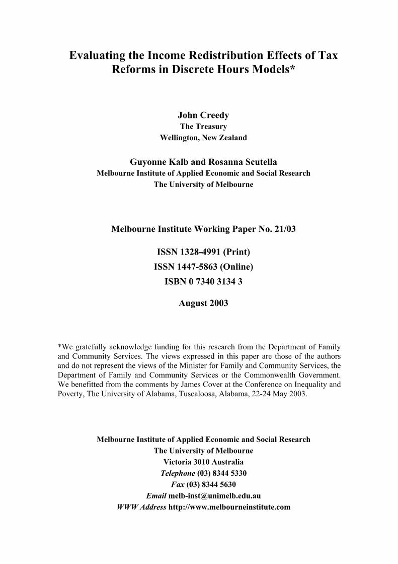
50, 000 draws.10 The convergence of mean income and the Gini inequality

measure are shown in Figures 2 and 3 respectively, for the case of n = 50.

Of course, this does not provide a practical approach that could be used

easily in microsimulation models, particularly for larger samples.11 However,

the associated stable values can be regarded as the ‘true’ values against

which the performance of the alternative approaches may be gauged in this

experiment.12

10Convergence takes place more quickly for the larger samples. However in many in-stances, the difference between the ‘true’ measure or mean and the measure or meanfound through the sampling approach is already small using many fewer draws even forthe smaller sample sizes.11For n = 500, taking 1000 repetitions, each of which involves 50, 000 random draws from

the 500 individuals’ hours distributions in the sample, the computation time is substantialat around four days.12There is one exception. It was demonstrated in section 2 that the use of average in-

comes, and the pseudo distribution, provide exact measures of the (appropriately weighted)mean, X. Where 10 draws are taken with the sampling approach, the mean from thepseudo distribution has been taken as the ‘true’ value, rather than that produced by50,000 draws.

12

0.3570

0.3575

0.3580

0.3585

0.3590

10 50 100 500 1000 5000 10000 50000 100000

random draw s

Gin

i coe

ffici

ent

Figure 3: Convergence For Gini Inequality Measure

3.2 Experimental Results

Tables 2 to 5 present the Monte Carlo results for three approaches comparing

deviations of the various approaches from the ‘true’ values for 1000 replica-

tions of the experiments.13 The first two methods are the expected income

method and the pseudo method. To explore the quality of the sampling ap-

proach when few draws are used, results are also produced for the sampling

approach with 10 draws. The use of 10 draws would be feasible in practice

and this number has been shown to be sufficient in other situations, such as

for example, Simulated Maximum Likelihood estimations.14

From all measures in the tables, it is clear that the pseudo method per-

forms much better than the expected income method. As shown analytically

for the variance, the two inequality measures are also always underestimated

by the expected income method and overestimated by the pseudo method

for samples with 50 or 100 individuals. This is as expected given that the ex-

13The experiment where a sample of 500 individuals is used took roughly four days torun. This involved drawing around 50,000,000 times (which is less than 108) from the500 hours distributions and computing averages across the 50,000 draws in each of the1000 replications. The exact measure for the same sample would involve 11500 differentcombinations which compared to the above drawing of 50,000 would require an enormousamount of time and be infeasible to carry out.14In Van Soest (1995), 5 draws seemed sufficient in one of the models estimated using

the Simulated Maximum Likelihood approach.

13

Table 2: Distribution of Differences from ‘True Value’: n=50

G A P0 P1 P2 X VAverage "true" values

0.33391 0.084995 0.115037 0.062394 0.047425 318.27 42674.11Use of each individual’s expected incomeMean -0.0336 -0.01199 -0.00526 9.18E-06 0.000372 -7303.94msea 0.001174 0.000148 0.000404 2.78E-05 1.26E-05 55194286Min -0.06056 -0.01993 -0.0821 -0.01785 -0.01328 -11498.1Max -0.01467 -0.00621 0.08906 0.025669 0.017747 -3531.46Use of pseudo distribution of incomeMean 0.004543 0.000275 0.001585 0.000748 0.000459 149.8281msea 0.000021 7.87E-08 0.000083 2.52E-06 8.82E-07 23739.04Min 0.001503 0.000079 -0.0253 -0.00373 -0.00267 4.246241Max 0.006876 0.000499 0.041592 0.006866 0.004414 314.5633Use of 10 random draws from possible distributionsMean -3.5E-05 -6.3E-06 0.000419 9.77E-05 7.14E-05 0.093905 -41.5227msea 0.000017 3.24E-06 0.000057 5.67E-06 3.1E-06 14.72302 2736878Min -0.01408 -0.0078 -0.02878 -0.01001 -0.00698 -11.542 -11104.1Max 0.011255 0.006216 0.049411 0.013506 0.012192 13.13847 9338.877Note a: mse stands for the mean squared error.



0.337054 0.085744 0.112875 0.062622 0.047801 318.11 43145.16Use of each individual’s expected incomeMean -0.03405 -0.01218 -0.00248 4.47E-05 0.000303 -7369.36msea 0.00118 0.00015 0.000194 1.23E-05 5.97E-06 55064023Min -0.0494 -0.0167 -0.05305 -0.01051 -0.00849 -10896.5Max -0.0194 -0.00813 0.062672 0.014378 0.008512 -4648.41Use of pseudo distribution of incomeMean 0.002273 0.000137 0.001157 0.000364 0.000237 74.73766msea 5.23E-06 1.94E-08 0.000039 7.18E-07 2.51E-07 5944.869Min 0.001236 0.000063 -0.02872 -0.00286 -0.0011 6.374102Max 0.003116 0.000244 0.025762 0.003468 0.002167 155.9846Use of 10 random draws from possible distributionsMean 1.91E-05 1.3E-05 0.000204 6.33E-05 3.97E-05 0.185203 31.26735msea 7.41E-06 1.55E-06 0.000022 2.54E-06 1.54E-06 7.814952 1479075Min -0.00835 -0.0045 -0.02395 -0.00516 -0.00408 -10.4604 -7314.95Max 0.009678 0.005463 0.022216 0.005611 0.004703 10.86006 5933.581Note a: mse stands for the mean squared error.

14



0.338943 0.086112 0.114024 0.063022 0.048044 317.97 43322.27Use of each individual’s expected incomeMean -0.03437 -0.01227 -0.00156 0.000181 0.000301 -7417.44msea 0.001191 0.000151 0.000108 5.11E-06 2.53E-06 55352057Min -0.04348 -0.01506 -0.03549 -0.00592 -0.00429 -10211.7Max -0.02511 -0.01005 0.03473 0.008382 0.005616 -5802.55Use of pseudo distribution of incomeMean 0.000911 5.38E-05 0.00057 0.00012 8.41E-05 29.81149msea 8.35E-07 3.05E-09 2.05E-05 1.75E-07 5.52E-08 1006.12Min 0.000678 0.000016 -0.01327 -0.00145 -0.0008 -10.9953Max 0.001146 0.000104 0.014827 0.001469 0.000927 85.59714Use of 10 random draws from possible distributionsMean -8.5E-05 -3.4E-05 2.62E-05 8.59E-06 -7.9E-07 0.029564 -10.633msea 3.25E-06 6.53E-07 9.87E-06 9.77E-07 5.83E-07 2.999281 595096.4Min -0.00574 -0.00267 -0.01384 -0.00367 -0.00302 -5.36467 -3252.28Max 0.004986 0.002338 0.016108 0.003251 0.002815 4.945107 2578.688Note a: mse stands for the mean squared error.

Table 5: Distribution of Differences from ‘True Value’: n=500G A P0 P1 P2 X V

Average "true" values0.340422 0.086779 0.115116 0.063697 0.048700 317.89 43486.24

Use of each individual’s expected incomeMean -0.03424 -0.01227 -0.00090 0.000426 0.000361 -7422.69msea 0.001177 0.000151 0.000077 2.96E-06 1.35E-06 55254183Min -0.04077 -0.01474 -0.02098 -0.00449 -0.00378 -8674.50Max -0.02718 -0.01000 0.02746 0.006148 0.004455 -6235.62Use of pseudo distribution of incomeMean 0.000454 0.000026 0.00021 0.000010 0.000020 14.33324msea 2.07E-07 7.68E-10 1.68E-05 5.30E-08 1.55E-08 260.649Min 0.000374 -0.000001 -0.01341 -0.000817 -0.000471 -20.8162Max 0.000543 0.000051 0.012726 0.000951 0.000596 42.10908Use of 10 random draws from possible distributionsMean 0.000072 3.12E-05 -5.84E-05 -3.02E-05 -7.50E-06 -0.001639 24.1993msea 1.55E-06 3.05E-07 6.84E-06 5.18E-07 3.12E-07 1.522162 256246.7Min -0.003427 -0.001878 -0.01053 -0.00198 -0.00184 -4.19253 -1608.05Max 0.004071 0.001896 0.010913 0.002368 0.001782 3.823399 1670.176Note a: mse stands for the mean squared error.

15

pected income understates the true income variability and the pseudo income

distribution overstates the income variability. However, for samples with 250

or 500 individuals, some negative differences between the "true" variance

and the variance from the pseudo method are found. This does not happen

very often and it can be explained by the fact that our "true" values which

are used as benchmarks in the experiment are approximations as well. As

the pseudo method improves with sample size, for n=250 or 500 the pseudo

method may sometimes get closer to the true value than the approximation

by 50,000 draws, causing the difference to be negative rather than positive.

This will happen more often for larger samples, making the pseudo method

a computationally very efficient approach with an approximate value close

to the true value.

The sampling method, using 10 draws, ranks in between the two other

methods. Only its mean is nearly always smaller (except for some mea-

sures when n equals 500), but that is because negative and positive values

partly offset each other in this approach, whereas the other two approaches

tend to over- or underestimate the true values. The pseudo method clearly

outperforms the sampling method with 10 draws except for the case of the

headcount measure P0. Nevertheless, on many occasions the accuracy of the

sampling method using only 10 draws would be considered sufficient.

With an increase in sample size, the methods tend to perform better

with the exception of the variance and inequality measures for the expected

income method. Using the latter method, the mean distance from the true

value does not change with sample size for G, A, P2 and V, whereas for P0 it

falls and for P1 it increases.15 Although the minimum and maximum values

move towards each other in the expected income method, a bias remains. In

the pseudo method and the sampling method with 10 draws, the minimum

and maximum value both move towards the true value. The pseudo method

improves faster with sample size than the sampling method with 10 draws.

15This result for V makes sense when considering equations (6) and (9) in section 2.

16

4 A Simulation Example

To illustrate the use of the pseudo method, a hypothetical reform of the

Australian tax and transfer system is examined. The Australian transfer

system is complex, with many different types of benefit, each with its set of

thresholds and taper (or withdrawal) rates, giving rise to highly nonlinear

budget constraints. The simulations described in this section replace all

existing basic social security benefits and additional payments such as rent

assistance, pharmaceutical allowance and family payments by a basic non-

taxable level of income. The existing direct tax structure (which includes

the Medicare levy and all tax rebates) is replaced with a constant marginal

tax rate on all taxable income (that is, all non-benefit forms of income).

The reform is simulated using the Melbourne Institute Tax and Transfer

Simulator (MITTS). The method of simulating labour supply responses to

tax reforms in MITTS is briefly described in subsection 4.1. The results of

the simulation are described in 4.2.

4.1 The Melbourne Institute Tax and Transfer Simu-lator

The behavioural responses in MITTS are based on the use of quadratic pref-

erence functions whereby the parameters are allowed to vary with an in-

dividual’s characteristics. These parameters have been estimated for five

demographic groups, which include married or partnered men and women,

single men and women, and sole parents.

For the couples in the labour supply estimation, two sets of discrete

labour supply points are used. Given that the female hours distribution

covers a wider range of part-time and full-time hours than the male distribu-

tion, which is mostly divided between non-participation and full-time work,

women’s labour supply is divided into 11 discrete points, whereas men’s

labour supply is represented by just six points. The couple’s joint labour

supply is estimated simultaneously, unlike the popular approach in which

female labour supply is estimated with the spouse’s labour supply taken as

17

exogenous.16 Thus for couples we have 66 possible joint labour supply com-

binations.

Rather than identifying a particular level of hours worked for each indi-

vidual after a policy change, a probability distribution is generated over the

discrete hours levels used.17 The behavioural simulations begin by taking

the discrete hours level for each individual that is closest to the observed

hours level. Then, given the parameter estimates of the quadratic prefer-

ence function (which vary according to a range of individual and household

characteristics), a random draw is taken from the distribution of the ‘error’

term. This draw is rejected if it results in an optimal hours level that differs

from the discretised value observed. The accepted drawings are then used

in the determination of the optimal hours level after the policy change. A

user-specified total number of ‘successful draws’ (that is, drawings which gen-

erate the observed hours as the optimal value under the base system for the

individual) are produced. In computing the transition matrices, which show

probabilities of movement between hours levels, the labour supply of each

individual before the policy change is fixed at the observed discretised value

and a number of transitions are produced for each individual, which is equal

to the number of successful draws specified.18 This gives rise to a probability

distribution over the set of discrete hours for each individual under the new

tax and transfer structure.16For those individuals in the data set who are not working, and who therefore do

not report a wage rate, an imputed wage is obtained. This imputed wage is based onestimated wage functions, which allow for possible selectivity bias, by first estimatingprobit equations for labour market participation. However, some individuals are excludedfrom the database if their imputed wage or their observed wage (obtained by dividing totalearnings by the number of hours worked) is unrealistic. The wage functions are reportedin Kalb and Scutella (2002) and the preference functions are in Kalb (2002): these areupdated versions of results reported in Creedy et al. (2002).17Some individuals, such as the self employed, the disabled, students and those over 65

have their labour supply fixed at their observed hours.18When examining average hours, the labour supply after the change for each individual

is based on the average value over the successful draws, for which the error term leads to thecorrect predicted hours before the change. This is equivalent to calculating the expectedhours of labour supply after the change, conditional on starting from the observed hoursbefore the change. In computing the tax and revenue levels, an expected value is alsoobtained after the policy change. That is, the tax and revenue for each of the accepteddraws are computed for each individual and an average over these is taken.

18

In some cases, the required number of successful random draws produc-

ing observed hours as the optimal hours cannot be generated from the model

within a reasonable number of total drawings. The number of random draws

tried, like the number of successful draws required, is specified by the user. If

after the total draws from the error term distribution, the model fails to pre-

dict the observed labour supply, the individual is left at their observed hours

in policy simulations. In the simulation example used here, the maximum

number of random draws is set to 5000 with 100 successful draws required.

4.2 Simulation Results

In the simulations examined in this section, a basic non-taxable level of in-

come replaces all existing basic social security benefits, and additional pay-

ments such as rent assistance, pharmaceutical allowance and family pay-

ments. The structure of the September 2001 tax and transfer system is used

as the pre-reform system. In the reform system, the existing tax structure

(which includes the Medicare levy and all tax rebates) is replaced with a

constant marginal tax rate on all taxable income (all non-benefit forms of

income). Basic income rates are set at the benefit levels as they were at

September 2001 with basic income levels varying for different groups in the

population reflecting the current situation. Characteristics that currently

entitle individuals to a pension are used to determine whether an individual

is entitled to a higher rate of basic income, which is referred to as the pension

rate. This group includes those of age pension age, those with a disability,

carers, veterans and sole parents. This payment is then differentiated by

marital status to reflect the economies of scale of larger households. The

remaining subset of the population receives a basic income level set at the

current allowance payment rates. These payments also differ by age, such

that single persons aged 16 or 17 years receive a lower basic income than older

individuals, with youths still living at home receiving a lower rate again and

those aged 60 years or over receive a higher level than 18 to 59 year olds.

Members of a couple are entitled to a lower payment rate each than the single

rate, reflecting economies of scale. To ensure revenue neutrality of the new

19

system compared to the 2001 system, the marginal tax rate required in this

system was 55 per cent.

The removal of means testing reduces the disincentives to work for those

on low incomes as it reduces the effective marginal tax rates significantly.

Lowering the marginal tax rate has two opposing effects. A lower tax rate

would induce substitution out of leisure and into work, as the price of leisure

is higher. However, at the same time net incomes are higher at lower levels

of labour supply, so some individuals/families may decide to reduce their

hours of work. The net result depends on relative preferences for leisure and

income. Higher taxes imposed at the high end of the income distribution

may have an adverse effect on the labour supply of higher income earners.

A summary of the estimated labour supply responses across demographic

groups is presented in Table 6 with the expected effect on net expenditure

reported in Table 7. The responses differ greatly across the groups. Singles

without children exhibit labour supply responses similar to those of married

men. However, single persons seem more likely to decrease participation

and to reduce their work effort as a result of a heavier tax burden than

married men. Married males are the least likely to decrease their labour

supply overall. Married women and sole parents tend to have larger income

effects thus having a greater tendency to move out of the labour force with

an increase in household income. In addition, the current payments to sole

parents are withdrawn very gradually and thus a tax rate of over fifty per

cent is higher than the effective marginal tax rate currently faced by them at

low income levels, reducing their incentive to work after the reform compared

with the 2001 system.

The adverse labour supply responses associated with a relatively high

marginal tax rate imposes a large increase in net government expenditure. A

large share of each individual’s income is paid in tax, so a reduction in labour

supply considerably reduces the revenue collected by the government. The

large reduction in the labour supply of married females increases net govern-

ment expenditure on couples. The higher tax rates on middle to high income

earners are not enough to offset the decrease in revenue resulting from the

decrease in participation and average working hours for this group. With a

20

Table 6: Behavioural Responses

Couples: Single Single SingleMen Women Men Women Parents

Workers (% base) 58.6 45.7 55.1 44.2 42.4Workers (% reform) 58.5 41.2 53.6 43.3 37.2Non-work —> work (%) 1.2 0.4 0.3 0.5 0.4Work —> non-work (%) 1.3 4.8 1.8 1.4 5.6Workers working more 1.3 0.3 0.0 0.1 2.0Workers working less 2.4 1.9 1.4 2.3 1.1Average hours change -0.2 -1.9 -0.9 -0.8 -0.6

Table 7: Net Expenditure Summary (in millions of dollars)

Couples Single Single SingleMen Women Parents Total

Fixed hours -4,024.5 1,735.8 2,042.8 -282.5 -528.4Variable hours 2,044.3 2,859.5 2,895.4 -172.0 7,627.2

general reduction in labour supply across all groups, net government expen-

diture increases after the reform when labour supply responses are taken into

account.

To examine the effects of this policy change on the distribution of in-

come before and after labour supply changes, three summary measures are

presented. First, two commonly used measures of inequality, the Gini coeffi-

cient and the Atkinson measure of inequality, are examined. As the reform

system provides relatively generous basic income levels financed by heavily

taxing the working population, it is not surprising that inequality is reduced

quite significantly after the reform; see Tables 8 and 9. Adjusting for labour

supply responses does not have a strong effect on the presented measures of

inequality in this case, since those who move out of the labour force were on

low wages.

For the analysis of poverty, values of the Foster, Greer and Thorbecke

Index of poverty are presented in Table 10. The inclusion of labour supply

responses in the simulation clearly affects the headcount measure, resulting

from the larger shift in median income. Taking into account labour supply

21

Table 8: Gini Coefficient by Income Unit Type

Fixed hours Variable hoursGroup Before After % change Before After % changeCouple 0.3103 0.2758 -11.1 0.3030 0.2701 -10.9Cple+dep 0.2460 0.1963 -20.2 0.2333 0.1857 -20.4Single Females 0.2925 0.2616 -10.6 0.2950 0.2609 -11.6Single Males 0.3297 0.2825 -14.3 0.3343 0.2839 -15.1Sole Parents 0.2154 0.2067 -4.0 0.2101 0.2029 -3.4all 0.3014 0.2654 -12.0 0.2980 0.2616 -12.2

responses results in more poverty than would otherwise be the case. This

effect becomes less pronounced when the extent of the poverty is taken into

account in the poverty gap and the Foster, Greer and Thorbecke measure of

poverty with α = 2.

5 Conclusions

This paper has compared alternative approaches to the measurement of in-

equality and poverty indices in the context of behavioural microsimulation

with discrete hours labour supply models. Special consideration is needed

because microsimulation modelling using a discrete hours approach does not

identify a particular level of hours worked for each individual after a policy

change, but generates a probability distribution over the discrete hours lev-

els used. This makes analysis of the distribution of income difficult because,

even for a small sample with a modest range of hours points, the range of

possible labour supply combinations becomes too large to handle.

The approaches examined include the use of an expected income level for

each individual. Alternatively, a simulated approach could be used in which

labour supply values are drawn from each individual’s hours distribution and

summary statistics of the distribution of income are calculated by taking the

average over each set of draws. Finally, the construction of a pseudo income

distribution was proposed. This uses the probability of a particular labour

supply value occurring (standardised by the population size) to refer to a

particular position in the pseudo income distribution.

22

Table 9: Atkinson Inequality Measures by Income Units

Fixed hours Variable hoursGroup Before After % change Before After % changeε = 0.1Couple 0.0155 0.0123 -20.6 0.0147 0.0117 -20.4Cple+dep 0.0106 0.007 -33.0 0.0095 0.0062 -34.7Single Females 0.0141 0.0112 -20.6 0.0145 0.0112 -22.1Single Males 0.0182 0.0136 -25.8 0.0188 0.0137 -27.1Sole Parents 0.0083 0.0077 -7.2 0.008 0.0075 -7.5all 0.0151 0.0117 -22.5 0.0148 0.0113 -23.0ε = 0.5Couple 0.0749 0.0597 -20.3 0.0711 0.0568 -20.1Cple+dep 0.0498 0.0332 -33.3 0.0448 0.0294 -34.4Single Females 0.0680 0.0540 -20.6 0.0697 0.0539 -22.7Single Males 0.0879 0.0646 -26.5 0.0906 0.0652 -28.0Sole Parents 0.0387 0.0360 -7.0 0.0373 0.0348 -6.4all 0.0724 0.0564 -22.1 0.0710 0.0546 -23.0ε = 1Couple 0.1429 0.1145 -19.8 0.1355 0.1091 -19.5Cple+dep 0.0934 0.0627 -32.9 0.0843 0.0560 -33.6Single Females 0.1300 0.1028 -20.9 0.1332 0.1020 -23.4Single Males 0.1686 0.1222 -27.5 0.1740 0.1232 -29.3Sole Parents 0.0711 0.0661 -7.0 0.0684 0.0641 -6.3all 0.1380 0.1078 -21.9 0.1355 0.1046 -22.8ε = 2Couple 0.2563 0.208 -18.9 0.2429 0.1981 -18.4Cple+dep 0.1684 0.1151 -31.7 0.1524 0.1037 -32.0Single Females 0.2383 0.1840 -22.7 0.2451 0.1814 -26.0Single Males 0.3114 0.2191 -29.7 0.3221 0.2202 -31.6Sole Parents 0.1218 0.1127 -7.5 0.1170 0.1098 -6.2all 0.2527 0.1968 -22.1 0.2501 0.1914 -23.5

23

Table 10: Alternative Poverty Measures

Fixed hours Variable hoursBefore After % Before After %

Poverty line50% median income $182.15 $198.28 $176.28 $221.20α = 0 (headcount)a

Couple 0.0157 0.0000 -100.0 0.0150 0.0490 227.3Cple+dep 0.0151 0.0000 -100.0 0.0173 0.0027 -84.4Single Females 0.0685 0.1177 71.8 0.0768 0.3980 418.1Single Males 0.0710 0.1137 60.1 0.0784 0.2798 256.9Sole Parents 0.0111 0.0000 -100.0 0.0035 0.0161 362.9all 0.0409 0.0547 33.7 0.0444 0.1724 288.3α = 1 (poverty gap)Couple 0.0054 0.0000 -100.0 0.0053 0.0017 -67.9Cple+dep 0.0031 0.0000 -100.0 0.0029 0.0001 -93.1Single Females 0.0224 0.0157 -29.9 0.0258 0.0420 62.8Single Males 0.0260 0.0103 -60.4 0.0299 0.0316 5.7Sole Parents 0.0005 0.0000 -100.0 0.0001 0.0002 100.0all 0.0135 0.0061 -54.8 0.0151 0.0177 17.2α = 2Couple 0.0021 0.0000 -100.0 0.0020 0.0001 -100.0Cple+dep 0.0007 0.0000 -100.0 0.0006 0.0000 -100.0Single Females 0.0096 0.0034 -64.6 0.0115 0.0080 -29.6Single Males 0.0121 0.0015 -87.6 0.0140 0.0054 -61.4Sole Parents 0.0000 0.0000 0.0 0.0000 0.0000 0.0all 0.0058 0.0012 -81.0 0.0067 0.0032 -52.2note a: a larger α indicates that larger poverty gaps are penalised more.

24

It was shown that the outcomes of various distributional measures using

the pseudo distribution method converge to their ‘true’ values as the sam-

ple size used in microsimulation increases. However, the method performs

well for a sample as small as 50 individuals. The pseudo method performs

better than the expected income method or the sampling approach with just

10 draws. The latter has a similar computational burden to the pseudo

approach. The feasibility of the pseudo approach is demonstrated in an il-

lustrative example where the labour supply responses and implications for

the distribution of income were examined for a hypothetical reform of the

Australian tax and transfer system.

25

Appendix: Inequality and Poverty MeasuresUsing the Different Approaches

This appendix lists the expressions for the inequality and poverty measures

used in this paper, for the alternative approaches.19

First, the Atkinson measure (for unit-relative inequality aversion) is, for

all combinations:

1−knXm=1


exp 1n

Pni=1 ln(yhim,i)

1n

Pni=1 yhim,i

The sampling approach is similar, where a sample is drawn from all possible

combinations and the probability of drawing a particular combination m is

equal to the probability ph1m,1ph2m,2...phnm,n. Using expected incomes:

1− exp1n

Pni=1 ln(

Pkh=1 phiyhi)

1n

Pni=1

Pkh=1 phiyhi

Using the pseudo approach:

1− exp1n

Pni=1

Pkh=1 phi ln(yhi)

1n

Pni=1

Pkh=1 phiyhi

Second, the Gini Coefficient for all combinations is expressed as:

n+ 1

n− 1 − 2knXm=1


Pni=1 ρlimyhlimmlim

n(n− 1) 1n

Pni=1 yhim,i

with lim indicating the index for the household with the ith ranked income in

the mth combination and ρlim = ρli−1,m + 1. Using expected incomes it is:

n+ 1

n− 1 − 2Pn

i=1 ρl∗iPk

h=1 phl∗i yhl∗i

n(n− 1) 1n

Pni=1

Pkh=1 phiyhi

with l∗i indicating the index for the household with the ith ranked expected

income and ρl∗i = ρl∗i−1 + 1. Using the pseudo method the Gini measure is:

n+ 1

n− 1 − 2Pn

i=1

Pkh=1 ρvh(i−1)+h,blh(i−1)+hpvh(i−1)+h,blh(i−1)+hyvh(i−1)+h,blh(i−1)+h

n(n− 1) 1n

Pni=1

Pkh=1 phiyhi

19Creedy (1996) and Deaton (1997) present a range of inequality and poverty measures,including those presented here.

26

with blh(i−1)+h indicating the index for the household with the (h(i−1)+h)th

ranked income within the nh possible incomes, vh(i−1)+h indicating the index

for the discrete hours point with the (h(i − 1) + h)th ranked income and

ρvh(i−1)+h,blh(i−1)+h = ρvh(i−1)+h−1,blh(i−1)+h−1 + pvh(i−1)+h,blh(i−1)+h.Third, the headcount measure for all combinations is:

knXm=1


n

nXi=1

1(yhim,i ≤ ypov,m)

where ypov,m = 0.5 × yhlimmlim and lim indicates the index for the household

with the ith ranked income in the mth combination, where i/n = 0.5. Using

expected income it is:nXi=1

1(kX

h=1

phiyhi ≤ ypov)

where ypov = 0.5×Pk

h=1 phl∗i yhl∗i with l∗i indicating the index for the household

with the ith ranked expected income, where i/n = 0.5. Using the pseudo

method it is:nXi=1

kXh=1

phi1(yhi ≤ ypov)

where ypov = 0.5× yvh(i−1)+h,blh(i−1)+hwith blh(i−1)+h indicating the index for thehousehold with the (h(i − 1) + h)th ranked income within the nh possible

incomes, vh(i−1)+h indicating the index for the discrete hours point with the

(h(i−1)+h)th ranked income, where h(i−1)+h indicates the income wherePh(i−1)+hk=1 pvk,blk = 0.5.Fourth, the Poverty Gap measure for all combinations is:

knXm=1


n

nXi=1

µ1− yhim,i

ypov,m

¶1(yhim,i ≤ ypov,m)

where ypov,m = 0.5× yhlimmlimwith lim indicating the index for the household


expected income it is:

nXi=1

Ã1−

Pkh=1 phiyhiypov

!1(

kXh=1

phiyhi ≤ ypov)

27




method it is:nXi=1

kXh=1

phi

µ1− yhi

ypov

¶1(yhi ≤ ypov)



(h(i−1)+h)th ranked income, where h(i−1)+h indicates the income wherePh(i−1)+hk=1 pvk,blk = 0.5.Fifth, the Foster, Greer and Thorbecke measure with α = 2, can be

expressed, for all combinations, as:

knXm=1


n

nXi=1

µ1− yhim,i

ypov,m

¶α

1(yhim,i ≤ ypov,m)

where ypov,m = 0.5× yhlimmlimwith lim indicating the index for the household


expected incomes it is:

nXi=1

Ã1−

Pkh=1 phiyhiypov

!α

1(kX

h=1

phiyhi ≤ ypov)




method it is:nXi=1

kXh=1

phi

µ1− yhi

ypov

¶α

1(yhi ≤ ypov)



(h(i−1)+h)th ranked income, where h(i−1)+h indicates the income wherePh(i−1)+hk=1 pvk,blk = 0.5.

28

References

[1] Creedy, J. (1996) Fiscal Policy and Social Welfare: An Analysis of Al-

ternative Tax and Transfer Systems. Edward Elgar, Cheltenham UK.

[2] Creedy, J. and Duncan, A.S. (2002) Behavioural microsimulation with

labour supply responses. Journal of Economic Surveys, 16, pp. 1-39.

[3] Creedy, J., Duncan, A.S., Scutella, R. and Harris, M. (2002) Microsim-

ulation Modelling of Taxation and The Labour Market: The Melbourne

Institute Tax and Transfer Simulator. Cheltenham: Edward Elgar.

[4] Deaton, A. (1997) The Analysis of Household Surveys; A Microecono-

metric Approach to Development Policy. The Johns Hopkins University

Press, Baltimore.

[5] Foster, J., Greer, J. and Thorbecke, E. (1984) A class of decomposable

poverty measures. Econometrica, 52, pp. 761-762.

[6] Gerfin, M. and Leu, R.E. (2003) The impact of in-work benefits on

poverty and household labour supply: a simulation study for Switzer-

land. Discussion Paper No. 762, IZA, Bonn.

[7] Kalb, G. (2002) Estimation of labour supply models for four separate

groups in the Australian population. Melbourne InstituteWorking Paper

No. 24/02, The University of Melbourne.

[8] Kalb, G. and Scutella. R. (2002) Estimation of wage equations in Aus-

tralia: allowing for censored observations of labour supply. Melbourne

Institute Working Paper No. 8/02, The University of Melbourne.

[9] Keane, M., and Moffitt, R. (1998) A structural model of multiple wel-

fare program participation and labour supply. International Economic

Review, 39, pp. 553-590.

[10] Van Soest, A. (1995) A structural model of family labor supply: a dis-

crete choice approach. Journal of Human Resources, 30, pp. 63-88.

29

Evaluating the Income Redistribution Effects of Tax ...

Documents

Transcript of Evaluating the Income Redistribution Effects of Tax ...