EU Ukraine Trade Liberalization Costs of Tariff Elimination Frey Olekseyuk

The EU-Ukraine trade liberalization:How much do the

costs of tariff elimination matter?

Miriam FREY12, Zoryana OLEKSEYUK3

1University of Regensburg2Osteuropa-Institut Regensburg3University of Duisburg-Essen

Contents

Abstract . . . . . . . . . . . . . . . . . . . . . . . . . . . . . . . . . . . . . . . . . . . . . . . . . . . . . . . . . . . . . . . . . . . . . . . . . . . . . . . . . . . . . iii

1 Introduction . . . . . . . . . . . . . . . . . . . . . . . . . . . . . . . . . . . . . . . . . . . . . . . . . . . . . . . . . . . . . . . . . . . . . . . . . . . . . . 1

2 Literature overview . . . . . . . . . . . . . . . . . . . . . . . . . . . . . . . . . . . . . . . . . . . . . . . . . . . . . . . . . . . . . . . . . . . . . . 2

3 Model description . . . . . . . . . . . . . . . . . . . . . . . . . . . . . . . . . . . . . . . . . . . . . . . . . . . . . . . . . . . . . . . . . . . . . . . . 3

4 Data and policy experiments . . . . . . . . . . . . . . . . . . . . . . . . . . . . . . . . . . . . . . . . . . . . . . . . . . . . . . . . . . . . . 6

5 Simulation results . . . . . . . . . . . . . . . . . . . . . . . . . . . . . . . . . . . . . . . . . . . . . . . . . . . . . . . . . . . . . . . . . . . . . . . . 10

5.1 Aggregate effects . . . . . . . . . . . . . . . . . . . . . . . . . . . . . . . . . . . . . . . . . . . . . . . . . . . . . . . . . . . . . . . . . 10

5.2 Disaggregate results . . . . . . . . . . . . . . . . . . . . . . . . . . . . . . . . . . . . . . . . . . . . . . . . . . . . . . . . . . . . . . 12

5.3 Robustness and sensitivity analysis . . . . . . . . . . . . . . . . . . . . . . . . . . . . . . . . . . . . . . . . . . . . . . . . 17

6 Summary and policy implications . . . . . . . . . . . . . . . . . . . . . . . . . . . . . . . . . . . . . . . . . . . . . . . . . . . . . . . . 20

A Appendix . . . . . . . . . . . . . . . . . . . . . . . . . . . . . . . . . . . . . . . . . . . . . . . . . . . . . . . . . . . . . . . . . . . . . . . . . . . . . . . . 23

List of Tables

Table 4.1: Shares for household disaggregation (in %) . . . . . . . . . . . . . . . . . . . . . . . . . . . . . . . . 7

Table 4.2: Model elasticities . . . . . . . . . . . . . . . . . . . . . . . . . . . . . . . . . . . . . . . . . . . . . . . . . . . . . . . . . . 7

Table 4.3: Calculated import tariffs . . . . . . . . . . . . . . . . . . . . . . . . . . . . . . . . . . . . . . . . . . . . . . . . . . . . 9

Table 5.1: Aggregate results . . . . . . . . . . . . . . . . . . . . . . . . . . . . . . . . . . . . . . . . . . . . . . . . . . . . . . . . . . 11

Table 5.2: Simulation results for different base years . . . . . . . . . . . . . . . . . . . . . . . . . . . . . . . . . . 17

Table 5.3: Robustness checks . . . . . . . . . . . . . . . . . . . . . . . . . . . . . . . . . . . . . . . . . . . . . . . . . . . . . . . . 19

Table A.1: Countries’ aggregation into trading regions . . . . . . . . . . . . . . . . . . . . . . . . . . . . . . . . . 23

Table A.2: Initial input and output structure of production sectors . . . . . . . . . . . . . . . . . . . . . . . 24

Table A.3: Factor intensity of production sectors . . . . . . . . . . . . . . . . . . . . . . . . . . . . . . . . . . . . . . . 25

Table A.4: Consumption shares (in %) . . . . . . . . . . . . . . . . . . . . . . . . . . . . . . . . . . . . . . . . . . . . . . . . 26

Table A.5: Disaggregate results . . . . . . . . . . . . . . . . . . . . . . . . . . . . . . . . . . . . . . . . . . . . . . . . . . . . . . . 27

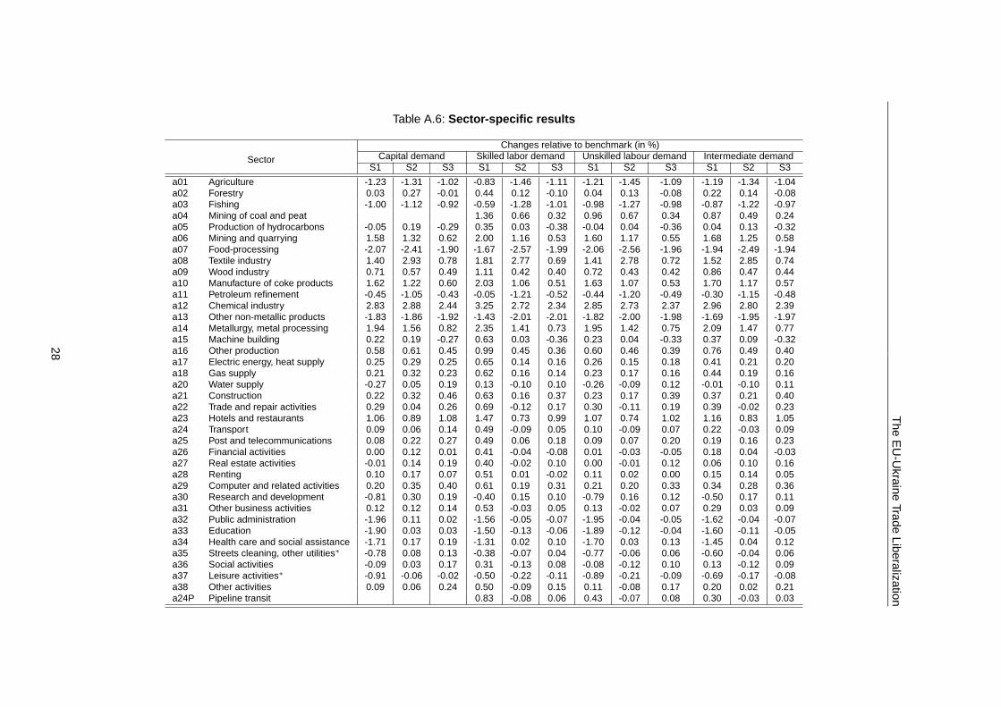
Table A.6: Sector-specific results. . . . . . . . . . . . . . . . . . . . . . . . . . . . . . . . . . . . . . . . . . . . . . . . . . . . . . 28

Table A.7: Public spending (UAH bn) . . . . . . . . . . . . . . . . . . . . . . . . . . . . . . . . . . . . . . . . . . . . . . . . . . 29

List of Figures

Figure 3.1: Model structure . . . . . . . . . . . . . . . . . . . . . . . . . . . . . . . . . . . . . . . . . . . . . . . . . . . . . . . . . . . . 4

Figure 4.1: Structure of Ukrainian commodity trade. . . . . . . . . . . . . . . . . . . . . . . . . . . . . . . . . . . . . 8

Figure 5.1: Regional structure of Ukrainian foreign trade . . . . . . . . . . . . . . . . . . . . . . . . . . . . . . . 13

Figure 5.2: Disaggregate results (change in %) . . . . . . . . . . . . . . . . . . . . . . . . . . . . . . . . . . . . . . . . 16

2

Abstract

The establishment of the currently negotiated Free Trade Agreement (FTA) between the EU andUkraine is the next significant step towards Ukraine’s deeper integration into the world economy,widely expected to result in additional welfare gains. As developing countries face some costsassociated with trade liberalization, this paper contributes to the literature by analyzing the effectsof the EU-Ukraine FTA taking into account the loss of tariff revenues as well as the changedeconomic conditions after Ukraine’s accession to the WTO in 2008. In particular, we calculatethe effects of a unilateral tariff elimination in a Computable General Equilibrium (CGE) modelfor Ukraine simulating three scenarios reflecting different means to compensate for the loss intariff revenues. It turns out to be important to take these costs into consideration while modelingtrade liberalization, as the results vary significantly across the scenarios. In general, we findthat tariff elimination has only a small impact on the country’s welfare because of the alreadystrongly reduced tariff rates after Ukraine’s WTO accession. The effects can even be negative ifthe country tries to refinance the trade liberalization costs by means of tax policy. According toour simulations the most welfare enhancing option would be the provision of financial support bythe EU, which is in fact suggested in the latest European Parliament resolution.

JEL-Classification: C68, F13, F15, H50, O52Keywords: Ukraine, EU, Trade, Integration, CGE, Public Spending

The EU-Ukraine Trade Liberalization

1 Introduction

After Ukraine’s accession to the WTO in 2008 the creation of a Free Trade Agreement(FTA) between Ukraine and its most important trading partner the European Union (EU)4

is the next significant and realistic step towards Ukraine’sdeeper integration into the worldeconomy. The WTO accession has already caused major changes especially in the fieldof tariff reductions but it was also considered to be a prerequisite for the negotiationson the deep and comprehensive FTA (DCFTA), which began in February 2008 withinthe framework of the Association Agreement (AA). So far there have been 21 rounds ofnegotiations and, despite of condemned political events inUkraine, the European Parlia-ment stated in its recent resolution that the EU-Ukraine AA should be rapidly initialled,preferably by the end of 2011. The signing of the agreement isintended for the first halfof 2012 and the ratification stage should be completed by the end of 2012.5

Theory suggests that trade liberalization is beneficial andthe problems as well as costsof reducing trade barriers are mostly neglected in literature. However, they should espe-cially be taken into consideration in case of developing countries like Ukraine. Reducedtariffs cause a loss of the tariff revenues and induce economic and social problems due todisruptions in agriculture. As these effects might lead to nations being worse off, devel-oping countries might decide not to liberalize foreign trade.6

In this paper we focus on one of the most obvious and importantcosts of trade liber-alization - the loss of tariff revenues. We analyze different scenarios simulating variousoptions to compensate the lost revenues. In particular, we calculate the effects of a uni-lateral import tariff elimination on the welfare and trade flows in a Computable GeneralEquilibrium (CGE) model for Ukraine.

One might wonder why in case of a bilateral agreement, only a unilateral tariff elimi-nation is examined. The reason for this is that according to Weisbrot and Baker (2002)” [. . .] most of the projected gains from trade liberalization do notcome from the removalof trade barriers in the industrialized countries - rather the biggest source of gains to de-veloping countries is the removal of their own barriers to trade.” To realize these gainsit is basically irrelevant whether the industrialized country - in our case the EU - alsoliberalizes its trade or not.

The paper is organized as follows. The next section providesan overview of the existingliterature. The structure of the model is described in section 3 followed by the specifica-tion of the data sources and the policy experiments. A detailed analysis of the resultsis given in section 5 including some robustness checks. The last section concludes withsome policy implications.

4To put it correctly, if the European Union would not be considered as one single tradingpartner, Russia would be on top.5See European Parliament (2011) available at http : //www.europarl.europa.eu/plenary/en/texts− adopted.html.6See Weisbrot and Baker (2002).

1


2 Literature overview

The different forms of Ukraine’s integration into the worldeconomy are widely evaluated.Most previous studies are devoted to the WTO accession. In theframework of a standardCGE model Pavel et al. (2004) simulate the full WTO accession ofUkraine including tar-iff reduction, improved market access and adjustments of domestic taxation and identifya significant welfare gain and an increase in real GDP. These findings are supported byJensen et al. (2005) who predict an overall welfare gain of 5.2% of Ukrainian consump-tion and a rise of real GDP by 2.4% in a modified model (e.g. somesectors produce underincreasing returns to scale). Kosse (2002) confirms that thetariff reduction is indeedthe most important part of the full WTO accession. She separately analyzes the impactof an import tariff reduction on national welfare and finds the WTO membership to bebeneficial for Ukraine.

Subsequent studies focus on Ukraine’s trade relations withthe EU, especially after theten Central and Eastern European countries joined the EU in 2004. An analysis of thedifferent FTAs between Ukraine and the EU shows that the DCFTA, which addition-ally incorporates the harmonization of the Ukrainian normsand standards, would havea stronger positive impact on Ukraine’s welfare compared tothe simple one where theoverall welfare effects are small or even slightly negative.7 In a more recent study Mal-iszewska et al. (2009) model the impact of the different FTAsbetween the five EuropeanNeighborhood Policy (ENP) countries (Armenia, Azerbaijan, Georgia, Ukraine and Rus-sia) and the EU. The conclusions are similar to the ones in theprevious study. Amongthe ENP countries, Ukraine gains most from the simple FTA with a net welfare increaseof 1.73%. But it could benefit even more from a DCFTA (increase ofwelfare by 5.83%).Francois and Manchin (2009) study the same question for the CIS region and Ukraineas a country study, but they find negative real income effectsfor the CIS and Ukraine (-0.83% and -2.12%, respectively) in case of the classical FTAsimulation and a decrease ofUkrainian real income by 0.4% even under the DCFTA scenario. The most recent studyon the Ukraine-EU FTA is done by von Cramon-Taubadel et al. (2010) for the WorldBank. Using the GTAP model and dataset they mainly focus on theagricultural sectorand find that a 50% reduction in all bilateral tariffs would only result in moderate gainsfor Ukraine and the EU. Note that the last two papers are some of the very few ones toconsider Ukraine’s final WTO commitments by simulating the changes after the acces-sion.

These studies do not state clearly how they deal with the costs resulting from the tariffelimination.8 This issue is addressed by Weisbrot and Baker (2002). They argue that onesubstantial problem in reducing trade barriers is the loss of revenues due to a reductionor elimination of tariffs. This especially applies to developing countries as tariff revenues

7See Emerson et al. (2006) and Ecorys and CASE-Ukraine (2007).8The general and mostly applied method to deal with reduced tariff revenues in a CGEmodel is to increase lump sum taxes. But this is an unrealistic assumption because lumpsum taxes are an artificial construct (see von Cramon-Taubadel et al. (2010)).

2


account for a considerable share of the national budget. Forinstance, due to the Ukrainiantreasury report9 the tariff revenues amount to 4.5% of the public budget. Following thisargument our paper contributes to the ongoing discussion intwo ways. First, it comple-ments the only very scarce research on the effects of the EU-Ukraine FTA incorporatingthe changed economic conditionsafter Ukraine’s WTO accession in 2008. Second, weexplicitly account for the loss of tariff revenues as one of the most important costs of tradeliberalization in case of a developing country and evaluatedifferent modes of compensa-tion for these losses.

3 Model description

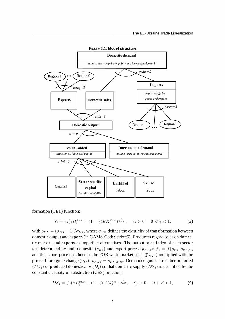
Our model updates and extends the static CGE model of Pavel et al. (2004). In additionto the updated database the modifications include the creation of new trading regions andproduction sectors, the disaggregation of the representative household into four types andthe implementation of sector-specific capital. It is implemented in GAMS/MPSGE10 andconsiders 38 sectors, four types of households, the government, investments and ninetrading regions. The structure of the model is shown in Figure 3.1.

The supply side of the Ukrainian economy is characterized bythe assumptions of per-fect competition and constant returns to scale. There are four factors of production: skilledand unskilled labor (ls,i), capital (ki) and sector-specific capital. Labor and capital (ex-cept sector-specific capital in the state-owned mining (a04) and pipeline transportation(a24P)) are perfectly mobile across sectors. The top nest ofthe production function ischaracterized by a Leontief-type structure:

yi = min{V Ai, IDi,j}, (1)

whereyi represents the total output of sector i (including domesticsales and exports),IDi,j is the intermediate demand for good j by industry i, andV Ai is the value added thatis given by the Cobb-Douglas function:

V Ai = c k(1−

∑

s αs,i)i

∏

s

lαs,i

s,i , 0 ≤ αs,i ≤ 1,∑

s

αs,i < 1, c > 0. (2)

The subscripts denotes the two types of labor: skilled and unskilled. Intermediate in-puts are either produced domestically or imported. Each firmuses a CES composite ofdomestic and imported intermediate inputs.11 Producers maximize profits subject to theirproduction technology.

Each sector is assumed to produce a single homogeneous product, which can be soldon domestic(Hi) or foreign(EXi) markets according to the constant elasticity of trans-

9The report of the Accounting Chamber of Ukraine for 2007 is available in ukrainian athttp : //www.ac− rada.gov.ua/control/main/uk/publish/article/1126693; jsessionid =65AD9325C838702DD8808F622567899D.

10See Rutherford (1999) and Boehringer et al. (2003).11See equation (4).

3


Figure 3.1: Model structure

Domestic demand

- indirect taxes on private, public and investment demand

- indirect taxes on intermediate demand

b b b

b b b

Region 1 Region 9

Domestic salesExports

Imports

- import tariffs by

Region 9Region 1Domestic output

Value Added

- direct tax on labor and capital

Intermediate demand

CapitalSector-specific

capital(in a04 and a24P)

Unskilled

labor

Skilled

labor

esdm=5

etreg=3

etdx=5

esreg=3

s = o

s_VA=1

goods and regions

formation (CET) function:

Yi = ψi(γHρEX

i + (1− γ)EXρEX

i )1

ρEX , ψi > 0, 0 < γ < 1, (3)

with ρEX = (σEX − 1)/σEX , whereσEX defines the elasticity of transformation betweendomestic output and exports (in GAMS-Code: etdx=5). Producers regard sales on domes-tic markets and exports as imperfect alternatives. The output price index of each sectori is determined by both domestic(pH,i) and export prices(pEX,i): p̂i = f(pH,i, pEX,i),and the export price is defined as the FOB world market price(pEX,i) multiplied with theprice of foreign exchange(pfx): pEX,i = pEX,ipfx. Demanded goods are either imported(IMj) or produced domestically(Dj) so that domestic supply(DSj) is described by theconstant elasticity of substitution (CES) function:

DSj = ψj(βDρIMj + (1− β)IMρIM

j )1

ρIM , ψj > 0, 0 < β < 1, (4)

4


with ρIM = (σIM − 1)/σIM , whereσIM defines the elasticity of substitution betweenimports and domestic goods (in GAMS-Code: esdm=5). This means that consumer pref-erences are modeled as Armington-style product differentiation.12 The domestic priceindex of each goodj is determined by the domestic sales price(pD,j), the import price(pIM,j) and the import tariff(τIM,j): pj = f(pD,j, pIM,j(1 + τIM,j)). The import priceequals the CIF world market price(pIM,j) multiplied with the price of foreign exchange(pfx): pIM,j = pIM,jpfx.

The consumption side is represented by public consumption,investment and intermedi-ate consumption as well as by final consumption of households. A representative house-hold derives utility from consumption of goods and servicesand finances its total con-sumption by income from labor (

∑

swsL) and capital endowments (rK) and by receivedtransfers from the government (TG

hh) and from abroad (T ahh). This means that the value of

total consumption of a representative household (ΣjCjpj(1 + τj))13 does not exceed theincome multiplied with the total share of consumption (θ, 0 < θ < 1):

∑

j

Cjpj(1 + τj) ≤ θ

[

∑

s

wsL+ rK + TGhh + T a

hh

]

(5)

The representative household of the model is disaggregatedinto four types according tothe poverty line and the place of residence14: non-poor urban and rural households, poorurban and rural households. Non-poor households are endowed with both capital andlabor (skilled and unskilled) whereas poor households are only endowed with unskilledlabor. All households receive transfers from the government and pay taxes and socialsecurity contributions. But only non-poor households receive transfers from abroad andsave a constant share of their income.

The government receives income from public capital endowments15 (rKp + rspKsp),revenue from direct (

∑

i τi(rki +∑

sws,ili)) and indirect taxes (∑

j τjpj(Cj + INVj +

IDj + Gj + EXj)), from import tariffs (∑

j,r τIM,j,rpIM,jIMj,r), transfers from abroad(T a

G) and from households (T hhG ). Direct taxes are modeled as sector-specific taxes on the

use of production factors (capital and labor). Indirect taxes, in contrast, are modeled asproduct-specific taxes on private (Cj), investment (INVj), intermediate (IDj) and public(Gj) demand as well as on exports (EXj). Import tariffs (τIM,j,r) are product-specific anddistinguished by region. Government’s income is used for savings (pinvSAV G), transfersto households (TG

hh) and to abroad (TGa ), and to provide public services16 (

∑

j pjGj). The

12This assumption is based on Armington (1969). See also Dervis et al. (1982), p. 221-223, 226-227.

13Cj is the consumption of good j and τj represents consumption tax rate for good j.14The poverty line is calculated following the methodology of the Ministry of Economy ofUkraine (available in Ukrainian at http : //zakon.rada.gov.ua/cgi− bin/laws/main.cgi?nreg = z0401− 02).

15Including capital income in state-owned sectors with sector-specific capital (rspKsp):mining and pipeline transportation (a04 and a24P).

16Consumption levels of public services are determined by a Cobb-Douglas function.

5


public budget constraint is given by:

rKp + rspKsp +∑

i τi(rki +∑

sws,ili) +∑

j τjpj(Cj + INVj + IDj +Gj + EXj)

+∑

j,r τIM,j,rpIM,jIMj,r + T aG + T hh

G (6)

= pinvSAVG + TG

hh + TGa +

∑

j pjGj.

Aggregate investment is modeled as a Cobb-Douglas compositeover all goodsj:

INV = ψ∏

j

INVφj

j , φj ≥ 0,∑

j

φj = 1, ψ > 0. (7)

The price index for one unit of the aggregate investment goodis given by: pinv =

f(pj(1+ τj)). The sum of public (SAV G) and private savings (SAV hh) equals aggregateinvestment:17

pinv(SAVG + SAV hh) = pinvINV. (8)

Equilibrium is defined by zero profits for producers, balanced budgets for householdsand the government, and by market clearing for all goods and factor markets. For equal-ization of the balance of payments, it must be valid that the CIF value of imports togetherwith transfers from the government to abroad (TG

a ) are equal to the FOB value of exportsplus transfers from abroad to households (T a

hh) and to the government (T aG):

∑

j

pIM,jIMj + TGa =

∑

i

pEX,iEXi + T ahh + T a

G. (9)

The price of foreign exchange(pfx) is chosen as the numeraire.This model description gives a picture of all economic flows among the agents and

does not represent the explicitly programmed algebraic equations as we use the MPSGEsubsystem, which automatically generates the equations ofthe model based on referenceprices, quantities and elasticities.18

4 Data and policy experiments

The base year of our analysis is 2007 as we try to avoid the influence of the world eco-nomic crises. The backbone of the model is formed by a Social Accounting Matrix(SAM)19 with 38 sectors. It was constructed with the data of the Ukrainian NationalAccounts and Input-Output Tables for 2007 at basic and consumer prices (publications

17We do not consider the current account balance in the model as the data set is adjustedin the way that there are no imbalances.

18See Rutherford and Paltsev (1999) and Rutherford (1999).19See Pyatt and Round (1985).

6


of the State Statistics Committee of Ukraine).20 A SAM must be a balanced matrix sothat the row sums equal the corresponding column sums. As theSAM for Ukraine wasnot balanced in the first version (due to inconsistency of data sources), we used a fewbalancing items in order to match all rows and columns.

Additional information on indirect taxes, subsidies and imports (separately for inter-mediate, private, public and investment demand) as well as information on services tradeflows are also taken from the publication of the State Statistics Committee of Ukraine.Labor remuneration is disaggregated with data from this source as well.

The consumption shares per household type and sector are calculated from the Derzhkom-stat21 household budget survey for 2007 covering more than 10,000 Ukrainian householdsand over 200 different commodity groups (COICOP classification). Using these data theshares of payments from households to government as well as the shares of transfers fromthe government to poor households in their total expenditures are computed. The respec-tive figures are listed in Table 4.1.

Table 4.1: Shares for household disaggregation (in %)type of household (h) non-poor urban non-poor rural poor urban poor rural

division of transfers from house-holds to government∗

74 14 2 10

shares of transfers from gov-ernment in household’s expendi-tures

35 35

∗Transfers include taxes and social contributions.

Table 4.2: Model elasticitiesParameter Value Description

s 0 Elasticity of substitution between value added and intermediate inputss_VA 1 Elasticity of substitution between primary factors: capital and laboresdm 5 Armington elasticity of substitution between imports and domestic goodsetdx 5 Elasticity of transformation between domestic production and exportsesreg 3 Elasticity of substitution between import originetreg 3 Elasticity of transformation between export destination

Source: Pavel (2004), p. 4.

All elasticities of substitution and transformation are taken from Pavel et al. (2004) andpresented in Table 4.2. Data on Ukrainian commodity trade flows are drawn from theUnited Nations Commodity Trade Statistics Database (Comtrade). These data were ag-gregated into 17 (b01-b017) commodity groups. We used different correspondence tables

20Concerning the sectoral structure two changes were made in the SAM compared tothe original Input-Output Table. The heat supply sector was added to the electric en-ergy sector (a17) and the pipeline transit of oil and gas (a24P) was separated from thetransportation sector.

21The State Statistics Committee of Ukraine.

7


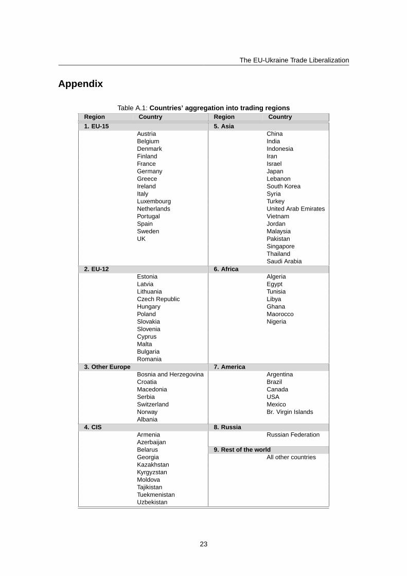
to convert the data from the HS96 into the KVED classification(Ukrainian classifica-tion which is based on NACE Rev.1). Ukraine’s exports and imports were grouped intothe following nine trading regions: EU-15, EU-12, other Europe, Asia, Africa, America,Commonwealth of Independent States (CIS), Russia and the rest of the world (ROW).The first eight regions include countries representing the key trading partners of Ukrainewith all other countries being summarized as the rest of the world.22 Figure 4.1 illustratesthe trade structure of Ukraine in 2007 and a detailed description of countries’ aggregationinto trading regions is given in Table A.1.

Figure 4.1: Structure of Ukrainian commodity trade

0 4 8 12 16 20

EU15

EU12

Other Europe

CIS

Russia

Asia

Africa

America

ROW

Exports in billions of US-$Imports in billions of US-$

Information on import tariffs is taken from the Law of Ukraine ”About the CustomsTariff of Ukraine” including all amendments made due to Ukraine’s accession to the WTOin 2008. The law includes three types of tariff rates (ad valorem, specific and mixed).First, the ad valorem equivalents of the specific and mixed tariffs were calculated.23 Theresulting tariff rates were transformed from the HS2000 into the KVED classificationusing again correspondence tables and applying different averages (simple, weighted,import-weighted). Table 4.3 shows the calculated import tariffs. With an import-weightedMFN tariff rate of 13.66 percent the food-processing, beverages and tobacco sector is themost protected one.

Different trade regimes are included in the model. Commoditytrade with Russia andother CIS countries is classified as free trade because of the existing FTA between Ukraineand the CIS countries.24 The MFN status is applied to trade with all other regions as theincluded countries are either members of the WTO or have bilateral trade agreements withUkraine to establish this trade regime.

22Exports and imports for the ROW region are obtained as a residual.23Following WTO et al. (2007), p.187-188.24The FTA was established in 1999.

8


Table 4.3: Calculated import tariffsSector SAM code Import-weighted MFN tariff∗

Agriculture b01 5,63Forestry, logging and related service activities b02 1,71Fishing b03 5,00Mining of coal and peat b04 0,00Production of hydrocarbons b05 0,50Mining and quarrying b06 2,23Food-processing b07 13,66Textile industry b08 8,06Wood industry b09 0,98Manufacture of coke products b10 1,61Petroleum refinement b11 1,64Chemical industry b12 3,71Other non-metallic products b13 7,07Metallurgy, metal processing b14 1,93Machine-building b15 3,09Other production b16 1,85Electric energy b17 3,50

∗These tariff rates apply to all trading regions except for Russia and CIS.

As the purpose of this paper is to quantify trade liberalization effects between Ukraineand the EU taking into account that lost tariff revenues25 have to be compensated, wemodel three different scenarios reflecting three possibilities to deal with this problem.All three scenarios have in common the elimination of the import tariffs in all commoditygroups for two regions in the model: EU-12 and EU-15. For all other regions the estimatedtariff rates are still valid.

In scenario 1 (S1) there is no possibility for the governmentto compensate the loss intariff revenues meaning that there is no endogenous adjustment. Therefore the eliminationof Ukraine’s import tariffs with respect to the EU goods has to result in a decrease of thegovernment spending.26

In contrast, in scenario 2 (S2) the government is assumed to use its power to enforce anincrease in the indirect tax rate meaning that the public consumption can be hold constant.

In scenario 3 (S3) we allow the government to gain additionalforeign aid as the EUintends to provide Ukraine with financial as well as technical and legal assistance.27 Thismeans that despite the decrease of tariff revenues neither the public expenditures have tobe reduced nor the indirect tax rate has to be increased.

25In the benchmark scenario tariff revenues amount to 4.03% of the public budget.26Note that this is not a realistic scenario as politicians might try to avoid such unpopularreforms.

27See European Parliament (2011), article 1(e).

9


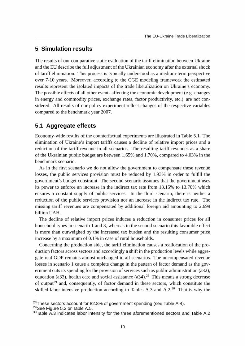
5 Simulation results

The results of our comparative static evaluation of the tariff elimination between Ukraineand the EU describe the full adjustment of the Ukrainian economy after the external shockof tariff elimination. This process is typically understood as a medium-term perspectiveover 7-10 years. Moreover, according to the CGE modeling framework the estimatedresults represent the isolated impacts of the trade liberalization on Ukraine’s economy.The possible effects of all other events affecting the economic development (e.g. changesin energy and commodity prices, exchange rates, factor productivity, etc.) are not con-sidered. All results of our policy experiment reflect changes of the respective variablescompared to the benchmark year 2007.

5.1 Aggregate effects

Economy-wide results of the counterfactual experiments are illustrated in Table 5.1. Theelimination of Ukraine’s import tariffs causes a decline ofrelative import prices and areduction of the tariff revenue in all scenarios. The resulting tariff revenues as a shareof the Ukrainian public budget are between 1.65% and 1.70%, compared to 4.03% in thebenchmark scenario.

As in the first scenario we do not allow the government to compensate these revenuelosses, the public services provision must be reduced by 1.93% in order to fulfill thegovernment’s budget constraint. The second scenario assumes that the government usesits power to enforce an increase in the indirect tax rate from13.15% to 13.70% whichensures a constant supply of public services. In the third scenario, there is neither areduction of the public services provision nor an increase in the indirect tax rate. Themissing tariff revenues are compensated by additional foreign aid amounting to 2.699billion UAH.

The decline of relative import prices induces a reduction inconsumer prices for allhousehold types in scenario 1 and 3, whereas in the second scenario this favorable effectis more than outweighed by the increased tax burden and the resulting consumer priceincrease by a maximum of 0.1% in case of rural households.

Concerning the production side, the tariff elimination causes a reallocation of the pro-duction factors across sectors and accordingly a shift in the production levels while aggre-gate real GDP remains almost unchanged in all scenarios. Theuncompensated revenuelosses in scenario 1 cause a complete change in the pattern offactor demand as the gov-ernment cuts its spending for the provision of services suchas public administration (a32),education (a33), health care and social assistance (a34).28 This means a strong decreaseof output29 and, consequently, of factor demand in these sectors, whichconstitute theskilled labor-intensive production according to Tables A.3 and A.2.30 That is why the

28These sectors account for 82.8% of government spending (see Table A.4).29See Figure 5.2 or Table A.5.30Table A.3 indicates labor intensity for the three aforementioned sectors and Table A.2

10


Table 5.1: Aggregate resultsVariable S0 S1 S2 S3

Tariff revenue (share of public budget, in %) 4.03 1.70 1.65 1.66Public services provision (change in %) - -1.93 0.00 0.00Indirect tax rate (weighted average, in %) 13.15 13.15 13.70 13.15Price index for households’ consumption composites(change in %):

- Urban households - -0.41 0.07 -0.39- Rural households - -0.47 0.10 -0.44- Urban poor households - -0.40 0.05 -0.37- Rural poor households - -0.44 0.08 -0.42

Real GDP (change in %) - 0.00 0.00 0.00Real factor return (change in %):

- Return to capital - 0.23 -0.08 0.10- Return to sector-specific capital in mining (a04) - 1.18 0.74 0.51- Return to sector-specific capital in pipeline transit (a24P) - 0.66 0.00 0.25- Wage rate for unskilled labor - 0.22 0.07 0.17- Wage rate for skilled labor - -0.17 0.08 0.19

Welfare per household type (Hicksian welfare index, changein %):

- Urban households - 0.48 -0.07 0.55- Rural households - 0.54 -0.09 0.61- Urban poor households - 0.56 0.00 0.50- Rural poor households - 0.69 -0.01 0.60

Consumption per household type (UAH bn):- Urban households 273.128 274.453 272.945 274.636- Rural households 96.059 96.579 95.971 96.644- Urban poor households 33.717 33.905 33.717 33.884- Rural poor households 26.715 26.898 26.712 26.876

Aggregate exports (UAH bn) 323.205 329.661 328.438 326.785Aggregate imports (UAH bn) 364.373 370.829 369.606 370.658Aggregate exports (change in %) - 2.00 1.62 1.11Aggregate imports (change in %) - 1.77 1.44 1.72Additional foreign aid (UAH bn) - - - 2.699

wage rate for skilled labor decreases in scenario 1 by 0.17% while unskilled labor andcapital receive higher factor returns of nearly 0.2%. In thesecond scenario, a shift infactor demand with unchanged public spending leads to a decrease of the return to capitalby 0.08%, while labor remuneration grows slightly by 0.07% for unskilled and by 0.08%for skilled labor meaning that capital would lose in this case. The higher returns to labor(skilled and unskilled) compared to the return to capital inthe third scenario together withfactor remuneration results of scenario 2 indicate a deepening of Ukraine’s specializationin the production of labor-intensive goods after trade liberalization.31

When interpreting the results concerning welfare, differing and partly opposing effectsshould be taken into consideration. Increases in factor remuneration and reduced con-

shows that the skilled labor demand is much higher in these industries compared to theunskilled labor type. These let us to conclude that public services are characterized byskilled labor-intensive production.

31Following the Heckscher-Ohlin and Stolper-Samuelson theorems, see Feenstra (2004),p. 15, 32, 174.

11


sumer prices are expected to stimulate consumption. In contrast, higher consumer pricesand reduced factor returns should have a negative impact on welfare. Therefore, the ques-tion which effect dominates should be answered separately for each of the scenarios. Theonly welfare reducing effect in scenario 1 is the decreasingwage rate for skilled labor.Nonetheless, the positive effects prevail and the non-poorhouseholds’ welfare is raisedon average by 0.51%, whereas for poor households a somewhat higher welfare increase(on average 0.63%) is found. In scenario 2, the reduced return to capital and the negativeeffect of higher consumer prices dominate and our simulation suggests no change (forurban poor households) or even a small reduction of consumption by nearly 0.08% fornon-poor and by approximately 0.01% for rural poor households. The stronger negativewelfare effect of non-poor households is caused by their higher tax burden compared tothe poor household types.32 In case of scenario 3, all effects point in the same direc-tion. There is a positive effect resulting from reduced consumer prices and all factors ofproduction gain a higher return compared to the benchmark scenario. These lead to anincrease in consumption and welfare of all household types.For non-poor households theaverage increase amounts to 0.58% and the respective value for the poor ones is 0.55%.

Not surprisingly, the strongest effect of the tariff elimination occurs in the foreign tradeflows of Ukraine. Aggregate imports rise in all scenarios by up to 1.77% (S1) and stimu-late an increase of exports in the range from 1.11% to 2%. Scenario 3 shows a somewhatlower rise of exports because foreign aid provides the economy with additional foreigncurrency needed for the purchase of increased imports.

Despite of changes in aggregate imports and exports, the fundamental trade structure ofUkraine with the model-specific regions remains almost unchanged as illustrated in Figure5.1. This means that there is no welfare reducing trade diversion as world prices remainunchanged in case of trade liberalization between the EU andUkraine.33 Nevertheless, theremoval of import tariffs between Ukraine and the EU leads toa small increase of importsfrom the EU member countries (EU-15 and EU-12) by 1.37 percentage points on averagefor all simulations (from 38.4% to 39.8%) while the import shares of all other regionsdecline slightly. The strongest fall in import shares is observed for Russia (by nearly0.53 percentage points). The results for the export structure suggest basically unchangedshares for all the regions.

5.2 Disaggregate results

Figure 5.2 and Table A.5 illustrate the changes in sectoral output, imports and exportsfor the different simulations. We observe that tariff elimination strongly favors Ukraine’schemical and textile industries, metallurgy, mining and quarrying and the manufacturingof coke products. These activities experience the strongest output increase in all simu-lations while a rise of production in sectors such as wood industry, mining of coal and

32See Table 4.1.33See Kemp and Wan (1976), Feenstra (2004), p.192-196 and WTO (2011), p. 100-102.

12


Figure 5.1: Regional structure of Ukrainian foreign trade

0

10

20

30

40

50

60

70

80

90

100

S0 S1 S2 S3

12.9

39.1

39.7

51.4

55.2

68.9

93.7

95.6100.0

12.7

38.3

39.0

50.3

54.1

68.2

93.9

95.7100.0

12.7

38.3

39.0

50.2

54.0

68.2

93.8

95.7100.0

12.7

38.3

38.9

50.2

54.0

68.2

93.8

95.7100.0

Imports

0

10

20

30

40

50

60

70

80

90

100

S0 S1 S2 S3

10.2

34.5

38.1

53.5

57.3

72.1

93.5

95.0100.0

10.2

34.5

38.1

53.6

57.4

72.2

93.5

95.0100.0

10.2

34.5

38.1

53.6

57.4

72.2

93.5

95.0100.0

10.2

34.4

38.1

53.5

57.3

72.2

93.5

95.0100.0

CIS Russia Africa Asia America

EU-12 EU-15 Other Europe ROW

Exports

peat and other production is still noteworthy. The output increase occurs in these sectorsbecause they are relatively unprotected in the benchmark (see Table 4.3) and benefit fromlower prices for intermediate goods which take over 50% of their total inputs (see Ta-ble A.2). Moreover, these winning sectors (except for manufacture of coke products andmining of coal) are export-oriented (see Table A.2) and gainadditionally from trade lib-eralization because the tariff-elimination-induced demand for imports leads to a foreignexchange outflow and, consequently, to a stimulation of exports. In addition to the afore-mentioned activities, hotels and restaurants benefit mostly among the service sectors ineach scenario because this sector is initially unprotected, exports nearly 51% of its outputand gains from the elimination of the highest import tariff (13.66%) in the food industry(i.e. cheaper intermediate inputs). On the other hand, food-processing and productionof non-metallic mineral products, agriculture, fishery andpetroleum refinement reducetheir output in all simulations because of a high initial level of protection and low exportshares. Concerning services, there is only in scenario 1 a strong output decrease in publicservices, education, health care and social assistance, leisure activities, streets cleaning aswell as in research and development what is driven by strongly reduced public spendingin these sectors34 due to the non-compensated revenue losses.

The development of exports and imports reflects the results for the output changes. Tar-

34See Table A.7.

13


iff removal leads to a rise of imports in the initially protected sectors (from agriculture upto electric energy) and across all scenarios35. Food-processing, production of non-metallicmineral products and agriculture have the highest degree ofprotection in the benchmarkand are thus on the top of the import increasing sectors. Thisrise of import demand is ac-companied in each simulation by an increase of exports in chemical and textile industry,metallurgy, wood industry, other production, mining and quarrying, machine building,and manufacture of coke products. In contrast, sectors as food-processing, production ofnon-metallic mineral products, petroleum refinement, agriculture and fishery reduce theirexports in every simulation. Concerning foreign trade in services, the changes in importsand exports are small as all service activities are unprotected in the benchmark equilib-rium. Nevertheless, hotels and restaurants as well as construction36 constitute exceptionswith a strong rise of exports by up to 1.72% and 1.44% (S1), respectively. Moreover, theaforementioned services with the decreased output experience also a decline of importsand exports in scenario 1 because of cuts in public spending.

The foreign trade results underline the specialization of Ukraine in labor-intensive goodsas the majority of activities with increased exports produce with intensive use of labor in-puts. As shown in Table A.3, these include chemical industry, metallurgy, wood industry,other production, machine building and manufacture of cokeproducts. On the other hand,losing sectors such as food-processing, petroleum refinement and agriculture are charac-terized by capital-intensive production.37 Hence, these results confirm the theoreticalexpectations that Ukraine, which is abundantly endowed with labor and poor in capitalendowments, specializes in labor-intensive goods on worldmarkets.

The results on factor and intermediate demand are presentedin Table A.6 and are con-sistent with the output changes. The sectors with extended production after simulationsraise their factor and intermediate demand as the rise of output needs an increased factorand intermediate input. On the contrary, demand for production factors and intermediateproducts declines in the sectors losing from trade liberalization38.

Slightly inconsistent results across scenarios are observed in such industries as forestryand production of hydrocarbons. These sectors reduce theiroutput and exports only inscenario 3, while imports rise. This phenomenon is related to the stronger import in-crease because of additional foreign aid in scenario 3. Moreover, we also observe somedifferences in prices, which lead to the presented results.In particular, import prices fallbecause of tariff elimination, but domestic supply prices rise in these industries because

35Except production of hydrocarbons in scenario 2 where we observe a slight decrease ofimports because of price changes in this sector: the relative import price of hydrocarbonsremains almost unchanged while the relative domestic supply price decreases.

36Construction gains from the elimination of import tariffs for non-metallic mineral products(initial value 7,07%) which allows for higher output and exports.

37Our data do not consider land as a separate production factor. This means that capitalincludes also land as an input for production.

38The strongest fall of factor and intermediate demand is observed in food-processingand production of non-metallic mineral products, agriculture, fishery and petroleum re-finement.

14


of increased factor remuneration.39 Concerning the third simulation, one notices that out-put changes for the initially protected sectors40 are lower compared to the other scenarios.The reason is the additional foreign currency provided withthe foreign aid which allowsfor increased import demand without a strong increase of exports and output.

39These sectors use much more labor and capital than intermediate inputs for production(see Table A.2), so that domestic supply prices increase with higher factor remuneration.

40These include the activities from agriculture up to electric energy and heat supply.

15

The

EU

-Ukraine

TradeLiberalization

Figure 5.2: Disaggregate results (change in %)

-3 -2 -1 0 1 2 3 4

Agriculture

Forestry

Fishing

Mining of coal and peat

Production of hydrocarbons

Mining and quarrying

Food-processing

Textile industry

Wood industry

Manufacture of coke products

Petroleum refinement

Chemical industry

Other non-metallic products

Metallurgy, metal processing

Machine building

Other production

Electric energy, heat supply

Gas supply

Water supply

Construction

Trade and repair activities

Hotels and restaurants

Transport

Post and telecommunications

Financial activities

Real estate activities

Renting

Computer and related activities

Research and development

Other business activities

Public administration

Education

Health care and social assistance

Streets cleaning, other utilities

Social activities

Leisure activities

Other activities

Pipeline transit

Output

-1 0 1 2 3 4 5

Exports

-4 0 4 8 12 16

S1

S2

S3

Imports

16


5.3 Robustness and sensitivity analysis

To check the robustness of our results with respect to the underlying data and elasticityvalues we repeated our simulations with some changes. Firstof all, we conducted thecounterfactual experiments with the data for 2004 examining whether the benchmark year2007 was arepresentativeyear and if the choice of another base year before the worldeconomic crisis would have led to significantly different results. Table 5.2 shows that thedifference between the results is small or even negligible.41 This confirms the robustnessof our results and supports the general experience in CGE modeling that the choice of thebase year has a minor impact on the robustness of simulation results.42

Table 5.2: Simulation results for different base years

Variable S0S1 S2 S3

2007 2004 2007 2004 2007 2004

Welfare per household type (Hicksian welfare in-

dex, change in %):

- Urban households - 0.48 0.53 -0.07 -0.13 0.55 0.57

- Rural households - 0.54 0.59 -0.09 -0.13 0.61 0.62

- Urban poor households - 0.56 0.65 0,00 -0.07 0.50 0.54

- Rural poor households - 0.69 0.86 -0.01 0.01 0.60 0.70

Price index for Households’ consumption com-

posites (change in %):

- Urban households - -0.41 -0.31 0.07 0.18 -0.39 -0.30

- Rural households - -0.47 -0.36 0.1 0.17 -0.44 -0.36

- Urban poor households - -0.4 -0.29 0.05 0.23 -0.37 -0.29

- Rural poor households - -0.44 -0.33 0.08 0.23 -0.42 -0.33

For examining the sensitivity of the represented results with respect to the elasticities ofsubstitution and transformation we ran 1000 simulations for each scenario with randomlydefined elasticity values taken from normal distribution centered at the initially assumedlevels.43 In particular, the elasticity of substitution between import origins (esreg) is cho-sen within the interval from 0.00001 to 6.0, while the Armington elasticity of substitutionbetween imports and domestic goods (esdm) as well as the elasticity of transformation be-tween domestic products and exports (etdx) range from 0.0000144 to 10.0.45 Furthermore,

41The only qualitative difference occurs in scenario 2 for rural poor households whichincrease their consumption by 0.01% in comparison with the reduction by 0.01% before.The reason is the benefit of these households from the higher increase (+0.22%) of thewage rate for unskilled labor (the sole production factor they are endowed with) in 2004.

42See Jensen et al. (2005), p. 25.43A comparable sensitivity analysis can be found in Jensen and Tarr (2011).44This value is chosen because Armington elasticities of zero are not theoretically possi-ble.

45We have also tested the elasticity of transformation between export destinations (etreg)but there is no influence on the welfare changes and other macroeconomic results.

17


in every simulation we allow for a random combination of the aforementioned elasticities.Table 5.346 summarizes the results of this robustness check for some macroeconomic

aggregates. For each variable and scenario we report the minimum, maximum and meanvalue out of 1000 simulations, the lower and upper bound of the 95% confidence inter-val.47 In addition, the table includes our initial simulation value and its relation to theconfidence band as well as the relative deviation of the minimum and maximum valuesin the robustness check from the initial result. We find that all our simulation results liewithin the 95% confidence interval and the robustness check values spread within an in-terval of less than 5% around the initial ones. Consequently,we consider our results to berobust with respect to the elasticity values. Nevertheless, the reported variables are moresensitive to different elasticity combinations in case of tariff elimination with endogenousadjustment of indirect taxes (scenario 2), as the lower and upper bound of the confidenceinterval suggest both, a possible decrease and increase of the price indices and welfarelevels of the poor household types. This means that such a tariff reform as a source offunds for trade liberalization could lead to small positiveor even negative welfare ef-fects for poor households depending on substitutability and transformability of Ukrainiangoods with foreign ones.

46All reported results except for deviations and trade flows are represented as raw simu-lation results and show changes relative to the benchmark values of 1.

47The 95% confidence interval is calculated for each scenario separately on the basis ofrobustness checks.

18

The

EU

-Ukraine

TradeLiberalization

Table 5.3: Robustness checksHicksian welfare index per household type Price index per household type Price index Trade flows (UAH bn)

urban rural urban poor rural poor urban rural urban poor rural poor for government exports imports

S1

Min. value 1.0041 1.0046 1.0043 1.0059 0.9932 0.9927 0.9932 0.9929 0.9962 324.5345 365.7025

Max. value 1.0053 1.0060 1.0069 1.0079 0.9981 0.9975 0.9984 0.9978 1.0000 334.9774 376.1454

Mean value 1.0048 1.0054 1.0056 1.0068 0.9959 0.9953 0.9960 0.9956 0.9985 328.9800 370.1480

Lower bound of the confidence inter-val (95%)

1.0043 1.0048 1.0045 1.0061 0.9937 0.9932 0.9937 0.9934 0.9967 325.2974 366.4654

Upper bound of the confidence inter-val (95%)

1.0052 1.0059 1.0066 1.0076 0.9978 0.9972 0.9981 0.9975 0.9998 333.5936 374.7616

Simulation value 1.0048 1.0054 1.0056 1.0069 0.9959 0.9953 0.9960 0.9956 0.9986 329.6608 370.8288

Simulation value within the confi-dence interval

+ + + + + + + + + + +

Min. deviation 0.0007 0.0008 0.0013 0.0010 0.0027 0.0026 0.0028 0.0027 0.0023 0.0156 0.0138

Max. deviation 0.0004 0.0006 0.0013 0.0010 0.0023 0.0022 0.0024 0.0022 0.0014 0.0161 0.0143

S2

Min. value 0.9988 0.9985 0.9982 0.9986 0.9976 0.9979 0.9973 0.9978 0.9987 323.3970 364.5650

Max. value 0.9999 0.9997 1.0018 1.0010 1.0035 1.0037 1.0033 1.0036 1.0027 333.6468 374.8148

Mean value 0.9993 0.9991 1.0000 0.9998 1.0007 1.0010 1.0005 1.0009 1.0010 327.7669 368.9349


0.9989 0.9986 0.9984 0.9987 0.9981 0.9984 0.9979 0.9983 0.9990 324.0303 365.1983


0.9998 0.9996 1.0014 1.0008 1.0032 1.0034 1.0030 1.0033 1.0025 332.2926 373.4606



+ + + + + + + + + + +

Min. deviation 0.0005 0.0006 0.0018 0.0013 0.0031 0.0030 0.0032 0.0031 0.0023 0.0153 0.0136

Max. deviation 0.0006 0.0006 0.0017 0.0011 0.0028 0.0027 0.0028 0.0028 0.0017 0.0159 0.0141

S3

Min. value 1.0048 1.0053 0.9933 1.0053 0.9935 0.9931 0.9935 0.9932 0.9982 323.3970 364.5650

Max. value 1.0160 1.0183 1.0063 1.0116 1.0390 1.0366 1.0404 1.0382 1.0437 333.6468 374.8148

Mean value 1.0056 1.0061 1.0049 1.0060 0.9963 0.9958 0.9964 0.9960 1.0004 327.7669 368.9349


1.0050 1.0055 1.0037 1.0054 0.9940 0.9936 0.9941 0.9938 0.9985 324.0303 365.1983


1.0060 1.0067 1.0060 1.0067 0.9985 0.9978 0.9987 0.9981 1.0021 332.2926 373.4606



+ + + + + + + + + + +

Min. deviation 0.0007 0.0008 0.0117 0.0007 0.0027 0.0025 0.0028 0.0026 0.0020 0.0153 0.0136

Max. deviation 0.0105 0.0122 0.0014 0.0055 0.0430 0.0412 0.0443 0.0425 0.0434 0.0159 0.0141

19


6 Summary and policy implications

The simulation of trade liberalization between Ukraine andthe EU confirms that it isindeed important to consider the costs of liberalization. Including different possibilitiesto compensate the loss in tariff revenues in a CGE model we calculate the effects ofUkraine liberalizing its trade with the EU unilaterally.

Briefly summarized, we obtain the following results: while real GDP is almost unaf-fected in all scenarios, welfare effects differ significantly ranging from -0.09% to 0.69%,depending on the mode of compensation. These differences are mainly driven by the riseof the consumer prices resulting from an increase in the indirect tax rate in scenario 2.As this is ruled out by assumption in the other scenarios, thetariff elimination would bewelfare enhancing in the uncompensated scenario (S1) and the aid-compensated scenario(S3), even though the magnitude varies. This reflects the reallocation of factors acrosssectors and the related change in demand and remuneration ofproduction factors, whichturn out differently in S1 and S3. Despite these differing results after the trade liberaliza-tion, an overall deepening of Ukraine’s specialization in the production of labor-intensivegoods can be identified. The majority of sectors, which gain from trade liberalizationbecause of an increase in production and exports, are labor-intensive. Among these arethe chemical industry, metallurgy, wood industry, machinebuilding and manufacture ofcoke products. Regarding trade, these sectors benefit from the tariff-elimination-induceddemand for imports which leads to a stimulation of exports. The strongest effect of thetariff elimination generally occurs in the foreign trade flows of Ukraine. At the same timethe fundamental trade structure remains almost unchanged.

Most previous studies on trade liberalization of Ukraine donot explicitly state howliberalization cost compensation is modeled. Moreover, the results differ significantly.Pavel et al. (2004), Jensen et al. (2005), Harbuzyuk and Lutz(2008), Maliszewska et al.(2009), Ecorys and CASE-Ukraine (2007) predict positive welfare effects (3-5%) whereasunchanged or even slightly lower welfare levels for Ukraineare found by Emerson et al.(2006), Francois and Manchin (2009). Our analysis suggeststhat one possible reasonfor the diverging results consists in different assumptions about the endogenous fiscaladjustments after trade liberalization. According to our simulations, negative as well aspositive welfare effects can result depending on the scenario. Though, our results differin terms of magnitude from those found in the previous literature probably because mostof the studies mentioned above use data on import tariffs applied beforeUkraine’s WTOaccession. This suggests that the elimination of already reduced tariff ratesafterUkraine’sWTO accession generates no or only slightly positive welfaregains because of the initiallylow level of protection.

Our study shows that the results are quite sensitive with respect to changes in fiscalpolicy. In particular, in our simulation the positive effects of the tariff elimination aremore than outweighed by the negative effects from the endogenous increase in indirecttaxes. This highlights the fact that the government should be prudent in funding the

20


liberalization costs by means of an increase in tax rates.Although we focus only on the effects of a simple EU-Ukraine FTA, the contracting

parties are in fact negotiating a DCFTA. This would imply evenhigher costs of tradeliberalization for Ukraine and the question of how to deal with this problem would beeven more important. Compensating these costs with foreign aid, as assumed in ourscenario 3, would enable Ukraine to gain even higher positive welfare effects as a resultof a DCFTA with the EU.

References

Armington, P. (1969). A Theory of Demand for Products Distuinguished by Place ofProduction.Internationally Monetary Fund Staff Paper 16, 159–176.

Boehringer, C., T. Rutherford, and W. Wiegard (2003). Computable General EquilibriumAnalysis: Opening a Black Box.ZEW Discussion Paper No. 03-56.

Dervis, K., J. De Melo, and S. Robinson (1982).General Equilibrium Models for Devel-opment Policy. Cambridge.

Ecorys and CASE-Ukraine (2007). Global Analysis Report for the EU-Ukraine TSIA,Ref. TRADE06/D01, DG-Trade.European Commission.

Emerson, M., T. Edwards, I. Gazizulin, M. Luecke, D. Mueller-Jentsch, V. Nanviska,V. Pyatnytskiy, A. Schneider, R. Schweikert, O. Shevtsov, and O. Shumylo (2006).The Prospect of Deep Free Trade between the European Union and Ukraine. Centrefor European Policy Studies (CEPS), Institut fuer Weltwirtschaft (IFW), InternationalCentre for Policy Studies (ICPS).

European Parliament (2011). European Parliament resolution of 1 December 2011containing the European Parliament’s recommendations to the Council, the Commis-sion and the EEAS on the negotiations of the EU-Ukraine Association Agreement.2011/2132(INI), P7_TA− PROV (2011)0545.

Feenstra, R. (2004).Advanced International Trade: Theory and Evidence. Princeton.

Francois, J. and M. Manchin (2009). Economic Impact of a Potential Free Trade Agree-ment (FTA) between the European Union and the Commonwealth ofthe IndependentStates.CASE Network Report No. 84.

Harbuzyuk, O. and S. Lutz (2008). Analyzing Trade Opening inUkraine: Effects of aCustoms Union with the EU.Econ Change Restruct 41, 221–238.

Jensen, J., P. Svensson, F. Pavel, L. Handrich, V. Movchan, and O. Betily (2005).Analysisof Economic Impacts of Ukraine’s Accession to the WTO: Overall Impact Assessment.Kyiv, Munic, Copenhagen.

21


Jensen, J. and D. Tarr (2011). Deep Trade Policy Options for Armenia: The Importanceof Services, Trade Facilitation and Standards Liberalization. The World Bank PolicyResearch Working Paper 5662.

Kemp, M. and H. Wan (1976). An Elementary Proposition concerning the Formation ofCustoms Unions.Journal of International Economics 6(1), 95–97.

Kosse, I. (2002). Using a CGE Model to Evaluate Impact Tariff Reductions in Ukraine.National University of Kyiv Mohyla Academy.

Maliszewska, M., I. Orlova, and S. Taran (2009). Deep Integration with the EU and itsLikely Impact on Selected ENP Countries and Russia.CASE Network Reports.

Pavel, F., I. Burakovsky, N. Selitska, and V. Movchan (2004).Economic Impact ofUkraine’s WTO Accession: First Results from a Computable General EquilibriumModel. Institute for Economic Research and Policy Consulting Working Paper, No.30.

Pyatt, G. and J. Round (1985). Social Accounting Matrices: A Basis for Planning.TheWorld Bank.

Rutherford, T. (1999). Applied General Equilibrium Modeling with MPSGE as a GAMSSubsystem: An Overview of the Modeling Framework and Syntax. ComputationalEconomics 14 (1/2).

Rutherford, T. and S. Paltsev (1999). From an Input-Output Table to a General Equilib-rium Model: Assessing the Excess Burden of Indirect Taxes in Russia.Department ofEconomics, University of Colorado, mimeo.

von Cramon-Taubadel, S., S. Hess, and B. Brümmer (2010). A Preliminary Analysis ofthe Impact of a Ukraine-EU Free Trade Agreement on Agriculture. The World BankPolicy Research Working Paper 5264.

Weisbrot, M. and D. Baker (2002). The Relative Impact of Trade Liberalization on De-veloping Countries.Center for Economic and Policy Research Briefing Paper.

WTO (2011). The WTO and Preferential Trade Agreements: From Co-Existence to Co-herence.World Trade Report 2011.

WTO, UNCTAD, and ITC (2007).World Tariff Profiles 2006. Switzerland.

22


Appendix

Table A.1: Countries’ aggregation into trading regionsRegion Country Region Country

1. EU-15 5. AsiaAustria ChinaBelgium IndiaDenmark IndonesiaFinland IranFrance IsraelGermany JapanGreece LebanonIreland South KoreaItaly SyriaLuxembourg TurkeyNetherlands United Arab EmiratesPortugal VietnamSpain JordanSweden MalaysiaUK Pakistan

SingaporeThailandSaudi Arabia

2. EU-12 6. AfricaEstonia AlgeriaLatvia EgyptLithuania TunisiaCzech Republic LibyaHungary GhanaPoland MaoroccoSlovakia NigeriaSloveniaCyprusMaltaBulgariaRomania

3. Other Europe 7. AmericaBosnia and Herzegovina ArgentinaCroatia BrazilMacedonia CanadaSerbia USASwitzerland MexicoNorway Br. Virgin IslandsAlbania

4. CIS 8. RussiaArmenia Russian FederationAzerbaijanBelarus 9. Rest of the worldGeorgia All other countriesKazakhstanKyrgyzstanMoldovaTajikistanTuekmenistanUzbekistan

23

The

EU

-Ukraine

TradeLiberalization

Table A.2: Initial input and output structure of production sectors

SectorInput (in %) Output (in %)

Intermediate Capital Sector-specific Skilled Unskilled Depreciation Total Domestic Exports Totaldemand demand capital demand labor demand labor demand sales

a01 Agriculture 58.23 31.63 0.00 3.55 5.68 0.92 100 92.45 7.55 100a02 Forestry 39.34 7.27 0.00 27.10 26.28 0.00 100 67.63 32.37 100a03 Fishing 72.08 9.94 0.00 8.22 9.76 0.00 100 97.22 2.78 100a04 Mining of coal and peat 38.85 0.00 15.98 25.71 19.27 0.18 100 93.48 6.52 100a05 Production of hydrocarbons 25.24 46.57 0.00 16.11 12.08 0.00 100 92.99 7.01 100a06 Mining and quarrying 51.85 27.40 0.00 10.62 7.96 2.16 100 73.09 26.91 100a07 Food-processing 73.86 10.95 0.00 7.35 5.51 2.34 100 78.33 21.67 100a08 Textile industry 47.51 20.68 0.00 12.07 9.05 10.69 100 28.80 71.20 100a09 Wood industry 73.36 9.03 0.00 10.07 7.54 0.00 100 71.20 28.80 100a10 Manufacture of coke products 77.11 13.87 0.00 4.00 3.00 2.02 100 95.79 4.21 100a11 Petroleum refinement 87.90 4.46 0.00 4.37 3.27 0.00 100 78.97 21.03 100a12 Chemical industry 78.83 9.92 0.00 6.43 4.82 0.00 100 46.33 53.67 100a13 Other non-metallic products 71.04 11.06 0.00 10.23 7.67 0.00 100 91.39 8.61 100a14 Metallurgy. metal processing 77.76 8.55 0.00 7.61 5.71 0.36 100 39.24 60.76 100a15 Machine building 73.47 9.43 0.00 9.77 7.32 0.00 100 55.08 44.92 100a16 Other production 70.34 6.69 0.00 10.27 7.70 4.99 100 76.60 23.40 100a17 Electric energy. heat supply 64.04 15.02 0.00 13.72 7.22 0.00 100 95.91 4.09 100a18 Gas supply 45.76 9.08 0.00 29.59 15.57 0.00 100 99.93 0.07 100a20 Water supply 60.50 0.68 0.00 25.43 13.39 0.00 100 99.61 0.39 100a21 Construction 68.41 8.89 0.00 11.67 11.04 0.00 100 99.22 0.78 100a22 Trade and repair activities 72.46 17.46 0.00 7.07 3.01 0.00 100 99.65 0.35 100a23 Hotels and restaurants 55.74 26.38 0.00 11.21 6.67 0.00 100 49.08 50.92 100a24 Transport 56.25 18.11 0.00 13.73 11.91 0.00 100 96.23 3.77 100a25 Post and telecommunications 47.58 30.69 0.00 14.08 7.65 0.00 100 90.10 9.90 100a26 Financial activities 31.18 36.05 0.00 29.96 2.81 0.00 100 96.10 3.90 100a27 Real estate activities 42.89 42.22 0.00 10.20 4.69 0.00 100 97.15 2.85 100a28 Renting 36.76 51.16 0.00 8.28 3.81 0.00 100 91.90 8.10 100a29 Computer and related activities 53.43 23.93 0.00 15.51 7.13 0.00 100 84.67 15.33 100a30 Research and development 22.43 9.26 0.00 53.82 8.18 6.32 100 79.97 20.03 100a31 Other business activities 51.90 18.89 0.00 20.01 9.20 0.00 100 93.41 6.59 100a32 Public administration 26.09 3.84 0.00 64.17 5.90 0.00 100 99.77 0.23 100a33 Education 26.91 7.25 0.00 54.39 11.46 0.00 100 99.46 0.54 100a34 Health care and social assistance 35.73 8.37 0.00 42.73 13.17 0.00 100 98.59 1.41 100a35 Streets cleaning. other utilities 55.59 7.38 0.00 20.22 16.81 0.00 100 99.50 0.50 100a36 Social activities 46.27 0.71 0.00 28.96 24.07 0.00 100 100.00 0.00 100a37 Leisure activities 51.07 15.93 0.00 26.53 6.47 0.00 100 89.84 10.16 100a38 Other activities 34.24 45.17 0.00 16.56 4.03 0.00 100 87.52 12.48 100

a24P Pipeline transit 81.24 0.00 9.93 4.73 4.10 0.00 100 0.00 100.00 100

24


Table A.3: Factor intensity of production sectors

Sector Capital demand (%) Labor demand (%) Factor intensity∗

a01 Agriculture 70.1 29.9 capital

a02 Forestry 21.9 78.1 labor

a03 Fishing 44.0 55.9 labor

a04 Mining of coal and peat 30.7 69.4 labor

a05 Production of hydrocarbons 59.5 40.5 capital

a06 Mining and quarrying 53.6 46.4 capital

a07 Food-processing 54.1 45.9 capital

a08 Textile industry 50.7 49.3 capital

a09 Wood industry 38.6 61.4 labor

a10 Manufacture of coke products 40.4 59.6 labor

a11 Petroleum refinement 55.1 44.9 capital

a12 Chemical industry 48.9 51.1 labor

a13 Other non-metallic products 44.9 55.1 labor

a14 Metallurgy. metal processing 44.2 55.8 labor

a15 Machine building 41.4 58.7 labor

a16 Other production 38.0 62.0 labor

a17 Electric energy. heat supply 42.6 57.4 labor

a18 Gas supply 31.5 68.5 labor

a20 Water supply 24.8 75.2 labor

a21 Construction 39.6 60.4 labor

a22 Trade and repair activities 58.1 41.9 capital

a23 Hotels and restaurants 56.0 44.0 capital

a24 Transport 46.1 53.9 labor

a25 Post and telecommunications 54.8 45.2 capital

a26 Financial activities 51.4 48.6 capital

a27 Real estate activities 63.7 36.3 capital

a28 Renting 72.2 27.8 capital

a29 Computer and related activities 48.5 51.5 labor

a30 Research and development 19.2 80.8 labor

a31 Other business activities 42.6 57.4 labor

a32 Public administration 13.8 86.2 labor

a33 Education 17.2 82.8 labor

a34 Health care and social assistance 23.3 76.7 labor

a35 Streets cleaning. other utilities 29.1 70.9 labor

a36 Social activities 23.2 76.8 labor

a37 Leisure activities 36.6 63.4 labor

a38 Other activities 62.7 37.3 capital

a24P Pipeline transit 46.1 53.9 labor

∗ The calculation of factor intensity for the model specific sectors accounts also for factor intensityof intermediate products (up to three stages).

25


Table A.4: Consumption shares (in %)

SectorConsumer

HouseholdsGovernment

urban rural urban poor rural poor

a01 Agriculture 10.54 9.19 12.90 7.98 0.90

a02 Forestry 0.09 0.64 0.24 0.62 0.22

a03 Fishing 1.67 1.64 1.73 1.28 0.00

a04 Mining of coal and peat 0.09 0.64 0.24 0.62 0.17

a05 Production of hydrocarbons 0.50 1.45 0.34 1.29 0.75

a06 Mining and quarrying 0.00 0.00 0.00 0.00 0.00

a07 Food-processing 40.97 42.36 48.78 36.49 0.28

a08 Textile industry 7.23 7.72 6.58 6.20 0.32

a09 Wood industry 0.54 0.44 0.50 0.31 0.03

a10 Manufacture of coke products 0.09 0.64 0.24 0.62 0.00

a11 Petroleum refinement 0.41 0.59 0.12 0.23 0.02

a12 Chemical industry 2.49 3.29 2.24 1.87 0.10

a13 Other non-metallic products 0.64 1.07 0.24 0.30 0.00

a14 Metallurgy. metal processing 0.62 1.06 0.22 0.28 0.00

a15 Machine building 3.40 4.31 1.17 1.17 0.46

a16 Other production 1.47 2.24 0.69 1.31 0.02

a17 Electric energy. heat supply 4.31 1.71 5.94 1.96 1.68

a18 Gas supply 1.53 2.51 3.70 2.18 0.12

a20 Water supply 0.66 0.24 1.25 0.31 0.25

a21 Construction 1.55 1.84 0.28 0.34 0.00

a22 Trade and repair activities 0.44 0.70 0.11 0.10 0.01

a23 Hotels and restaurants 2.66 1.24 1.07 0.56 0.20

a24 Transport 1.71 1.11 1.36 0.56 3.18

a25 Post and telecommunications 2.75 1.67 2.56 1.01 0.17

a26 Financial activities 5.70 7.84 1.90 2.96 0.00

a27 Real estate activities 1.36 0.23 1.34 0.05 1.93

a28 Renting 1.39 0.08 0.80 0.06 0.00

a29 Computer and related activities 0.00 0.00 0.00 0.00 0.01

a30 Research and development 0.00 0.00 0.00 0.00 2.63

a31 Other business activities 0.00 0.00 0.00 0.00 0.11

a32 Public administration 0.00 0.00 0.00 0.00 31.08

a33 Education 1.61 0.93 1.18 0.47 29.31

a34 Health care and social assistance 1.23 1.61 0.99 0.78 22.44

a35 Streets cleaning. other utilities 0.40 0.03 0.66 27.64 0.92

a36 Social activities 0.00 0.00 0.00 0.00 0.00

a37 Leisure activities 1.04 0.22 0.23 0.11 2.68

a38 Other activities 0.90 0.76 0.42 0.32 0.01

Total 100 100 100 100 100

26


Table A.5: Disaggregate results

Sector

Changes relative to benchmark (in %)Output Exports Imports

S1 S2 S3 S1 S2 S3 S1 S2 S3

a01 Agriculture -1.19 -1.34 -1.04 -0.78 -0.78 -0.47 6.62 6.28 6.59

a02 Forestry 0.22 0.14 -0.08 0.32 0.07 -0.47 2.70 2.99 3.39

a03 Fishing -0.87 -1.22 -0.97 -0.09 -0.48 -0.41 0.33 0.02 0.47

a04 Mining of coal and peat 0.87 0.49 0.24 0.43 0.05 -0.19 1.37 1.00 0.73

a05 Production of hydrocarbons 0.04 0.13 -0.32 -0.34 0.38 -0.72 0.45 -0.13 0.12

a06 Mining and quarrying 1.68 1.25 0.58 2.13 1.83 0.92 1.50 0.86 0.59

a07 Food-processing -1.94 -2.49 -1.94 -0.89 -1.32 -0.99 13.45 12.58 13.64

a08 Textile industry 1.52 2.85 0.74 3.56 5.24 2.62 3.11 2.48 3.25

a09 Wood industry 0.86 0.47 0.44 2.46 1.99 1.75 0.31 0.06 0.38

a10 Manufacture of coke products 1.70 1.17 0.57 1.58 1.11 0.45 2.74 2.15 1.62

a11 Petroleum refinement -0.30 -1.15 -0.48 -0.17 -1.52 -0.42 0.98 0.91 0.92

a12 Chemical industry 2.96 2.80 2.39 5.68 5.53 4.94 1.60 1.37 1.54

a13 Other non-metallic products -1.69 -1.95 -1.97 -0.78 -1.11 -1.29 9.31 9.10 9.28

a14 Metallurgy, metal processing 2.09 1.47 0.77 2.83 2.11 1.25 1.32 1.11 1.03

a15 Machine building 0.37 0.09 -0.32 2.20 1.94 1.21 1.36 1.01 1.41

a16 Other production 0.76 0.49 0.40 2.33 1.90 1.64 1.27 1.27 1.42

a17 Electric energy, heat supply 0.41 0.21 0.20 0.42 0.12 0.00 0.39 0.30 0.42

a18 Gas supply 0.44 0.19 0.16 0.74 0.24 -0.06 0.14 0.14 0.39

a20 Water supply -0.01 -0.10 0.11 0.29 -0.58 -0.17 -0.30 0.40 0.38

a21 Construction 0.37 0.21 0.40 1.44 1.10 1.19 -0.70 -0.69 -0.39

a22 Trade and repair activities 0.39 -0.02 0.23 0.32 0.18 0.04 0.42 -0.26 0.38

a23 Hotels and restaurants 1.16 0.83 1.05 1.72 1.34 1.50 -0.55 -0.75 -0.33

a24 Transport 0.22 -0.03 0.09 0.22 -0.03 -0.09 0.12 -0.05 0.20

a25 Post and telecommunications 0.19 0.16 0.23 0.64 1.00 0.56 -0.36 -0.87 -0.17

a26 Financial activities 0.18 0.04 -0.03 0.03 0.13 -0.57 0.33 -0.06 0.56

a27 Real estate activities 0.06 0.10 0.16 -0.01 0.12 0.08 0.14 0.08 0.26

a28 Renting 0.15 0.14 0.05 -0.28 0.42 -0.26 0.67 -0.19 0.42

a29 Computer and related activities 0.34 0.28 0.36 0.90 0.87 0.68 -0.42 -0.52 -0.09

a30 Research and development -0.50 0.17 0.11 0.41 0.28 0.07 -1.85 0.01 0.18

a31 Other business activities 0.29 0.03 0.09 0.66 0.43 0.10 -0.13 -0.42 0.08

a32 Public administration -1.62 -0.04 -0.07 -0.86 -0.60 -0.47 -2.36 0.53 0.34

a33 Education -1.60 -0.11 -0.05 -1.10 -0.81 -0.52 -2.10 0.60 0.43

a34 Health care and social assistance -1.45 0.04 0.12 -0.37 0.05 0.47 -2.54 0.03 -0.24

a35 Streets cleaning, other utilities∗ -0.60 -0.04 0.06 -0.17 -0.46 0.07 -1.02 0.38 0.05

a36 Social activities 0.13 -0.12 0.09

a37 Leisure activities∗ -0.69 -0.17 -0.08 -0.50 -0.36 -0.46 -0.92 0.07 0.38

a38 Other activities 0.20 0.02 0.21 0.34 0.16 0.29 0.01 -0.17 0.11

a24P Pipeline transit 0.30 -0.03 0.03 0.30 -0.03 0.03

strong negative changes strong positive changes∗a35: sewage, refuse disposal; a37 includes recreational, entertainment, cultural and sporting activities.

27

The

EU

-Ukraine

TradeLiberalization

Table A.6: Sector-specific results

Sector

Changes relative to benchmark (in %)Capital demand Skilled labor demand Unskilled labour demand Intermediate demand

S1 S2 S3 S1 S2 S3 S1 S2 S3 S1 S2 S3

a01 Agriculture -1.23 -1.31 -1.02 -0.83 -1.46 -1.11 -1.21 -1.45 -1.09 -1.19 -1.34 -1.04a02 Forestry 0.03 0.27 -0.01 0.44 0.12 -0.10 0.04 0.13 -0.08 0.22 0.14 -0.08a03 Fishing -1.00 -1.12 -0.92 -0.59 -1.28 -1.01 -0.98 -1.27 -0.98 -0.87 -1.22 -0.97a04 Mining of coal and peat 1.36 0.66 0.32 0.96 0.67 0.34 0.87 0.49 0.24a05 Production of hydrocarbons -0.05 0.19 -0.29 0.35 0.03 -0.38 -0.04 0.04 -0.36 0.04 0.13 -0.32a06 Mining and quarrying 1.58 1.32 0.62 2.00 1.16 0.53 1.60 1.17 0.55 1.68 1.25 0.58a07 Food-processing -2.07 -2.41 -1.90 -1.67 -2.57 -1.99 -2.06 -2.56 -1.96 -1.94 -2.49 -1.94a08 Textile industry 1.40 2.93 0.78 1.81 2.77 0.69 1.41 2.78 0.72 1.52 2.85 0.74a09 Wood industry 0.71 0.57 0.49 1.11 0.42 0.40 0.72 0.43 0.42 0.86 0.47 0.44a10 Manufacture of coke products 1.62 1.22 0.60 2.03 1.06 0.51 1.63 1.07 0.53 1.70 1.17 0.57a11 Petroleum refinement -0.45 -1.05 -0.43 -0.05 -1.21 -0.52 -0.44 -1.20 -0.49 -0.30 -1.15 -0.48a12 Chemical industry 2.83 2.88 2.44 3.25 2.72 2.34 2.85 2.73 2.37 2.96 2.80 2.39a13 Other non-metallic products -1.83 -1.86 -1.92 -1.43 -2.01 -2.01 -1.82 -2.00 -1.98 -1.69 -1.95 -1.97a14 Metallurgy, metal processing 1.94 1.56 0.82 2.35 1.41 0.73 1.95 1.42 0.75 2.09 1.47 0.77a15 Machine building 0.22 0.19 -0.27 0.63 0.03 -0.36 0.23 0.04 -0.33 0.37 0.09 -0.32a16 Other production 0.58 0.61 0.45 0.99 0.45 0.36 0.60 0.46 0.39 0.76 0.49 0.40a17 Electric energy, heat supply 0.25 0.29 0.25 0.65 0.14 0.16 0.26 0.15 0.18 0.41 0.21 0.20a18 Gas supply 0.21 0.32 0.23 0.62 0.16 0.14 0.23 0.17 0.16 0.44 0.19 0.16a20 Water supply -0.27 0.05 0.19 0.13 -0.10 0.10 -0.26 -0.09 0.12 -0.01 -0.10 0.11a21 Construction 0.22 0.32 0.46 0.63 0.16 0.37 0.23 0.17 0.39 0.37 0.21 0.40a22 Trade and repair activities 0.29 0.04 0.26 0.69 -0.12 0.17 0.30 -0.11 0.19 0.39 -0.02 0.23a23 Hotels and restaurants 1.06 0.89 1.08 1.47 0.73 0.99 1.07 0.74 1.02 1.16 0.83 1.05a24 Transport 0.09 0.06 0.14 0.49 -0.09 0.05 0.10 -0.09 0.07 0.22 -0.03 0.09a25 Post and telecommunications 0.08 0.22 0.27 0.49 0.06 0.18 0.09 0.07 0.20 0.19 0.16 0.23a26 Financial activities 0.00 0.12 0.01 0.41 -0.04 -0.08 0.01 -0.03 -0.05 0.18 0.04 -0.03a27 Real estate activities -0.01 0.14 0.19 0.40 -0.02 0.10 0.00 -0.01 0.12 0.06 0.10 0.16a28 Renting 0.10 0.17 0.07 0.51 0.01 -0.02 0.11 0.02 0.00 0.15 0.14 0.05a29 Computer and related activities 0.20 0.35 0.40 0.61 0.19 0.31 0.21 0.20 0.33 0.34 0.28 0.36a30 Research and development -0.81 0.30 0.19 -0.40 0.15 0.10 -0.79 0.16 0.12 -0.50 0.17 0.11a31 Other business activities 0.12 0.12 0.14 0.53 -0.03 0.05 0.13 -0.02 0.07 0.29 0.03 0.09a32 Public administration -1.96 0.11 0.02 -1.56 -0.05 -0.07 -1.95 -0.04 -0.05 -1.62 -0.04 -0.07a33 Education -1.90 0.03 0.03 -1.50 -0.13 -0.06 -1.89 -0.12 -0.04 -1.60 -0.11 -0.05a34 Health care and social assistance -1.71 0.17 0.19 -1.31 0.02 0.10 -1.70 0.03 0.13 -1.45 0.04 0.12a35 Streets cleaning, other utilities∗ -0.78 0.08 0.13 -0.38 -0.07 0.04 -0.77 -0.06 0.06 -0.60 -0.04 0.06a36 Social activities -0.09 0.03 0.17 0.31 -0.13 0.08 -0.08 -0.12 0.10 0.13 -0.12 0.09a37 Leisure activities∗ -0.91 -0.06 -0.02 -0.50 -0.22 -0.11 -0.89 -0.21 -0.09 -0.69 -0.17 -0.08a38 Other activities 0.09 0.06 0.24 0.50 -0.09 0.15 0.11 -0.08 0.17 0.20 0.02 0.21a24P Pipeline transit 0.83 -0.08 0.06 0.43 -0.07 0.08 0.30 -0.03 0.03

28


Table A.7: Public spending (UAH bn)

SectorBenchmark Changes

S0 S1 S2 S3

b01 Agriculture 1.1630 -0.0224 0.0032 0.0024

b02 Forestry 0.2800 -0.0057 0.0003 -0.0002

b03 Fishing 0.0000 0.0000 0.0000 0.0000

b04 Mining of coal and peat 0.1849 -0.0039 -0.0012 -0.0001

b05 Production of hydrocarbons 0.7818 -0.0163 -0.0059 0.0001

b06 Mining and quarrying 0.0000 0.0000 0.0000 0.0000

b07 Food-processing 0.3128 -0.0050 0.0000 0.0016

b08 Textile industry 0.3700 -0.0030 0.0038 0.0048

b09 Wood industry 0.0360 -0.0006 0.0000 0.0001

b10 Manufacture of coke products 0.0000 0.0000 0.0000 0.0000

b11 Petroleum refinement 0.0220 -0.0004 -0.0001 0.0000

b12 Chemical industry 0.1179 -0.0011 0.0010 0.0014

b13 Other non-metallic products 0.0030 0.0000 0.0000 0.0000

b14 Metallurgy. metal processing 0.0050 -0.0001 0.0000 0.0000

b15 Machine building 0.5338 -0.0068 0.0025 0.0043

b16 Other production 0.0190 -0.0003 0.0000 0.0001

b17 Electric energy. heat supply 1.7160 -0.0355 -0.0142 -0.0002

b18 Gas supply 0.1250 -0.0025 -0.0007 0.0000

b20 Water supply 0.2660 -0.0054 -0.0019 -0.0001

b21 Construction 0.0000 0.0000 0.0000 0.0000

b22 Trade and repair activities 0.0170 -0.0004 -0.0001 0.0000

b23 Hotels and restaurants 0.2430 -0.0047 -0.0003 0.0003

b24 Transport 4.0790 -0.0845 0.0033 0.0000

b25 Post and telecommunications 0.2090 -0.0041 0.0002 0.0002

b26 Financial activities 0.0000 0.0000 0.0000 0.0000

b27 Real estate activities 2.4060 -0.0502 -0.0008 0.0003

b28 Renting 0.0000 0.0000 0.0000 0.0000

b29 Computer and related activities 0.0090 -0.0002 0.0000 0.0000

b30 Research and development 3.3970 -0.0636 0.0042 0.0006

b31 Other business activities 0.1380 -0.0028 0.0002 0.0000

b32 Public administration 40.0770 -0.7725 -0.0039 -0.0198

b33 Education 37.8030 -0.7456 -0.0158 -0.0250

b34 Health care and social assistance 28.9320 -0.5374 0.0294 0.0289

b35 Streets cleaning. other utilities 1.1880 -0.0236 0.0001 0.0004

b36 Social activities 0.0000 0.0000 0.0000 0.0000

b37 Leisure activities 3.4470 -0.0702 0.0020 -0.0015

b38 Other activities 0.0130 -0.0003 0.0000 0.0000

b24P Pipeline transit 0.0000 0.0000 0.0000 0.0000

29

EU Ukraine Trade Liberalization Costs of Tariff Elimination Frey Olekseyuk

Documents

Transcript of EU Ukraine Trade Liberalization Costs of Tariff Elimination Frey Olekseyuk