
Etude des instabilités dans les puits activés par gas-lift · v Résumé (Étude des...
138
HAL Id: pastel-00001938 https://pastel.archives-ouvertes.fr/pastel-00001938 Submitted on 6 Nov 2006 HAL is a multi-disciplinary open access archive for the deposit and dissemination of sci- entific research documents, whether they are pub- lished or not. The documents may come from teaching and research institutions in France or abroad, or from public or private research centers. L’archive ouverte pluridisciplinaire HAL, est destinée au dépôt et à la diffusion de documents scientifiques de niveau recherche, publiés ou non, émanant des établissements d’enseignement et de recherche français ou étrangers, des laboratoires publics ou privés. Etude des instabilités dans les puits activés par gas-lift Laure Sinegre To cite this version: Laure Sinegre. Etude des instabilités dans les puits activés par gas-lift. Mathematics [math]. École Nationale Supérieure des Mines de Paris, 2006. English. <pastel-00001938>
Transcript of Etude des instabilités dans les puits activés par gas-lift · v Résumé (Étude des...

HAL Id: pastel-00001938https://pastel.archives-ouvertes.fr/pastel-00001938
Submitted on 6 Nov 2006
HAL is a multi-disciplinary open accessarchive for the deposit and dissemination of sci-entific research documents, whether they are pub-lished or not. The documents may come fromteaching and research institutions in France orabroad, or from public or private research centers.
L’archive ouverte pluridisciplinaire HAL, estdestinée au dépôt et à la diffusion de documentsscientifiques de niveau recherche, publiés ou non,émanant des établissements d’enseignement et derecherche français ou étrangers, des laboratoirespublics ou privés.
Etude des instabilités dans les puits activés par gas-liftLaure Sinegre
To cite this version:Laure Sinegre. Etude des instabilités dans les puits activés par gas-lift. Mathematics [math]. ÉcoleNationale Supérieure des Mines de Paris, 2006. English. <pastel-00001938>

N° attribué par la bibliothèque
|__|__|__|__|__|__|__|__|__|__|
T H E S E
pour obtenir le grade de Docteur de l’Ecole des Mines de Paris
Spécialité “Mathématiques et Automatique”
présentée et soutenue publiquement par Laure SINEGRE
le 20 septembre 2006
Etude des instabilités dans les puits activés par gas-lift
Directeur de thèse : Nicolas PETIT
Jury :
M. Rodolphe SEPULCHRE........................ Président du jury M. Bjarne FOSS....................................................Rapporteur M. Jean-Pierre RICHARD ....................................Rapporteur M. Pierre LEMETAYER ....................................... Examiteur M. Nicolas PETIT ......................................Directeur de thèse


Laure Sinègre
DYNAMIC STUDY OF
UNSTABLE PHENOMENA
STEPPING IN GAS-LIFT
ACTIVATED WELLS
Laure Sinègre
École Nationale Supérieure des Mines de Paris, Centre Automatique etSystèmes, 60, Bd. Saint-Michel, 75272 Paris Cedex 06, France.E-mail : [email protected]
Key words and phrases. — Process control, dynamic systems, limitcycles, switching system, gas-lifted Well, density-wave, stabilization,distributed parameters model.
Mots clés. — Contrôle de procédés, systèmes dynamiques, cyclelimite, système à switch, puits activés en gas-lift, density-wave,stabilisation, modèles à paramètres distribués.
28th September 2006

DYNAMIC STUDY OF UNSTABLE
PHENOMENA STEPPING IN GAS-LIFT
ACTIVATED WELLS
Laure Sinègre

iv
Abstract. — Gas-lifted wells often present unstable behaviors that can-not be described by hydrostatic laws. In this thesis, we aim at analyzingthe well dynamics, especially when its production is irregular. We endup by designing control solutions.
We begin with a brief description of the gas-lift activation technique.The negative impact of instabilities on oil production is underlined. Twomain mechanisms are at birth of the unstable behaviors. On-site realtime records serve as illustrative examples. We explain the first mech-anism, well referenced in the literature, thanks to mass balances equa-tions. Analyzing the vector field properties allows us to interpret theobserved phenomenon as a limit cycle. Then, we expose the main contri-bution of this thesis. It lies in the description and analysis of the secondmechanism. We show that the instability arises from out-of-phase effectsinduced by the propagation delay in the well. A distributed parametermodel is used. Then, we gather our results and present a complete andcompact model of the well dynamics. This model is a first order stablesystem interconnected with a distributed parameters system. Thanks tothe small gain theorem, the instabilities root-causes appear as two pos-sibly positive feedback loops. This model inspires the design of controlsolutions that suit the physical structure of the well. Moreover, these so-lutions fit with the operational constraints. Realistic simulation resultsillustrate the efficiency of our strategies. Some of the solutions have beentested on line on a production site. Some of the obtained results arepresented.

v
Résumé (Étude des instabilités dans les puits activés par gas-lift)
Les puits pétroliers activés par gas-lift sont souvent sujet à des com-portements instables qui ne peuvent être décrits par les lois de l’hydro-statique. L’objectif du travail présenté dans ce mémoire est l’analysede la dynamique de ces puits, en particulier lorsqu’ils produisent parà-coups. Elle aboutit à la conception de solutions de contrôle adaptées.
Nous commençons par décrire brièvement les principes de l’activationdes puits par gas-lift et soulignons l’impact très négatif des instabilitéssur les volumes de pétrole produits. Il existe deux principaux mécan-ismes susceptibles d’engendrer ces productions par à-coups. Nous lesmettons en évidence à partir d’enregistrements temps-réel issus de sitesde production. Le premier mécanisme, connu dans la littérature, estexpliqué grâce à des bilans de masses. Nous montrons, grâce à une anal-yse des propriétés du champ de vecteurs, que ce phénomène s’interprètegéométriquement comme un cycle limite. La principale contribution dece mémoire consiste en la description et l’analyse du second mécanisme,très mal connu auparavant. Nous montrons que le retard lié aux tempsde propagation des fluides dans le puits induit le déphasage à l’originede cette instabilité. L’étude de ces deux instabilités se poursuit parla présentation d’un modèle complet et compact de la dynamique dupuits. Il s’agit de l’interconnection d’un système du premier ordre stableavec un système à paramètres distribués. Il permet d’attribuer, grâceau théorème des petits gains, la cause des instabilités observées à deuxboucles de rétroaction potentiellement positives. Ce modèle nous permetde développer des solutions de contrôle, inspirées de la structure physiquedu puits et respectant les contraintes opérationnelles. L’efficacité de cesstratégies est illustrée par des résultats de simulations réalistes. Une par-tie des solutions a également été testée, en ligne, sur site de production.Certains résultats obtenus, très encourageants, sont présentés.


REMERCIEMENTS
Je remercie chaleureusement Rodolphe Sepulchre, président du jury,Jean-Pierre Richard et Bjarne Foss, rapporteurs de ma thèse.
Je tiens à remercier Pierre Lemétayer. Mine de savoir et d’expérience,il a soutenu le projet depuis le début. Sans sa conviction et sa ténacité ja-mais les tests sur site de production n’auraient pu avoir lieu. Je remercieégalement tout le personnel du site de production pour sa disponibil-ité. Je remercie Valérie Larrose-Martinez qui a très bien su gérer madélicate situation administrative et m’a ainsi évité bien des tracasseries.Merci à ceux qui ont permis à cette thèse d’exister, Marc Souche et YvesGuénard.
Un grand merci à Mme Le Gallic dont l’efficacité et la gentillesse m’ontété, à maintes reprises, d’un grand secours. Je remercie François Chap-lais, Pierre Rouchon, Philippe Martin et Laurent Praly pour l’intérêtqu’ils ont porté à ce travail. Enfin bon courage à mes compagnons deroute, Erwan, David, Mazyar et Silvère.
Merci à ceux, et tout particulièrement Jonathan, qui ont supporté sansbroncher mes moments de découragement, mes sautes d’humeur et milleet une présentations sur le gas-lift.
Je souhaite remercier mon directeur de thèse, Nicolas Petit, qui m’asuivie pendant ces cinq dernières années. Enfin suivie... poussée plutôt,guidée surtout. Merci de m’avoir fait confiance. Merci d’avoir toujoursété là. Je vais regretter votre enthousiasme pour les clés à molette, lesgrands scientifiques, les engins volants, le théorème des petits gains et lesbaklavas.

CONTENTS
Remerciements . . . . . . . . . . . . . . . . . . . . . . . . . . . . . . . . . . . . . . . . . . . . . . . . vii
Introduction . . . . . . . . . . . . . . . . . . . . . . . . . . . . . . . . . . . . . . . . . . . . . . . . . . . . 3
1. Process description and problematicDescription du procédé et problématique . . . . . . . . . . . . . . 13
1.1. Operations description . . . . . . . . . . . . . . . . . . . . . . . . . . . . . . . . . . . . 141.2. Operating conditions and efficiency . . . . . . . . . . . . . . . . . . . . . . . . 18
2. A dynamical system approach to the study of instabilitiesUne approche dynamique de l’analyse des instabilités . . 25
2.1. The casing-heading instability . . . . . . . . . . . . . . . . . . . . . . . . . . . . . . 262.2. The Density wave instability . . . . . . . . . . . . . . . . . . . . . . . . . . . . . . 452.3. Global study of unstable phenomena . . . . . . . . . . . . . . . . . . . . . . 65
3. Control solutionsSolutions de contrôle . . . . . . . . . . . . . . . . . . . . . . . . . . . . . . . . . . . . . . 79
3.1. State of the art . . . . . . . . . . . . . . . . . . . . . . . . . . . . . . . . . . . . . . . . . . . . 813.2. Controlling the tubing dynamics using gas inlet as input . . 84

2 CONTENTS
3.3. Controlling the tubing dynamics using the production chokeas input . . . . . . . . . . . . . . . . . . . . . . . . . . . . . . . . . . . . . . . . . . . . . . . . . . 90
3.4. Controlling the well dynamics using production choke as input. . . . . . . . . . . . . . . . . . . . . . . . . . . . . . . . . . . . . . . . . . . . . . . . . . . . . . . . . . . . 98
Conclusion . . . . . . . . . . . . . . . . . . . . . . . . . . . . . . . . . . . . . . . . . . . . . . . . . . . . . . 105
A. OLGAr2000 simulations settings . . . . . . . . . . . . . . . . . . . . . . . . 111
B. Nomenclature . . . . . . . . . . . . . . . . . . . . . . . . . . . . . . . . . . . . . . . . . . . . . . 113
List of figures . . . . . . . . . . . . . . . . . . . . . . . . . . . . . . . . . . . . . . . . . . . . . . . . . . 117
Bibliography . . . . . . . . . . . . . . . . . . . . . . . . . . . . . . . . . . . . . . . . . . . . . . . . . . . . 123

INTRODUCTION
Contexte. — Le pétrole est une ressource stratégique. Énergie essen-tielle dans de nombreux secteurs tels que les transports et l’industrie,il représente un enjeu à la fois économique et géopolitique. La criseactuelle du marché de l’énergie, la troisième du genre, apparaît prop-ice aux développements technologiques. La croissance de la demande enChine et en Inde, conjuguée à la montée des nationalismes pétroliers (telsqu’au Venezuela et en Bolivie, par exemple) entraîne une tension accruesur le marché du pétrole. Le prix du baril a doublé pour atteindre plus desoixante dollars en moins de deux ans. Cette flambée est alimentée par lespectre du manque de réserves et par les tensions géopolitiques. Ce con-texte est très favorable aux développements technologiques. D’un côté ilest nécessaire de produire plus et mieux. De l’autre le prix du baril aug-mentant, les budgets alloués aux projets à long terme sont conséquentscar les investissements sont plus facilement rentabilisés.
Ordres de grandeurs. — Si les variations du prix de l’or noir et lesconséquences économiques qu’elles induisent paraissent familières, sonextraction et le fonctionnement des installations restent mystérieux sousbien des aspects. Les formes sous lesquelles le pétrole se présente varientbeaucoup d’un champ à l’autre, la profondeur à laquelle il faut forer oula quantité de barils produits aussi. Il est donc assez difficile de définirdes ordres de grandeurs généraux. On peut néanmoins dire qu’un puits

4 INTRODUCTION
typique a une profondeur d’un à deux kilomètres et un diamètre de l’ordred’une dizaine de centimètres, que les pressions et les températures en jeuau niveau du réservoir sont de l’ordre d’une ou deux centaines de barspour l’un et d’une centaine de degrés pour l’autre et qu’un réservoirest supposé contenir quelques milliards de barils de pétrole. Un puitspeut produire jusqu’à plusieurs centaines de barils par jour et un champconsiste généralement en plusieurs centaines de puits. Pour se faire uneidée correcte des enjeux il faut également savoir qu’une grande partiedes réserves estimées de pétrole se trouve en mer à plusieurs kilomètresde profondeur et dans des régions parfois hostiles ou difficiles d’accès,comme en mer du Nord ou en Alaska par exemple. Il faut égalementinsister sur les disparités. En effet le champ d’Elgin Franklin en mer duNord est caractérisé par un réservoir à plus de 1000 bar et 200 oC et estdonc très loin des ordres de grandeurs moyens.
Activation de la production. — Au début de la production d’unpuits la pression du réservoir suffit fréquemment à propulser les hydrocar-bures jusqu’à la surface. C’est une phase de production dite "naturelle"qui, suivant les caractéristiques du réservoir, peut durer de quelques àde nombreuses années. Malheureusement en expulsant les effluents versla surface, le réservoir tend à se dépressuriser jusqu’à n’être plus capablede contrebalancer le poids de la colonne de liquide dans le puits. Il fautalors recourir à des moyens de production alternatifs, appelés moyensd’activation. Leur but peut être de maintenir le réservoir sous pressionou de tenter de diminuer le poids de la colonne liquide.
Gas-lift. — Parmi les moyens les plus fréquemment utilisés on trouvel’activation par pompe. Il peut s’agir de ce que l’on appelle des "têtesde cheval" à cause de leur forme particulière. On trouve égalementl’activation par gas-lift. Le gaz est injecté au fond du puits, il peut alorsêtre utilisé pour pousser le liquide ou pour s’y mêler de façon à dimin-uer la masse volumique moyenne. Au total, cette activation par gas-liftconcerne plus de 53% des puits produisant significativement, c’est-à-direplus de dix barils par jour (chiffres issus de [41, p6]). Dans ce mémoire,nous nous intéressons exclusivement à ce mode de production.

INTRODUCTION 5
Évolution du puits. — La plupart du temps, il est possible d’estimerl’évolution de la production d’un champ de pétrole. Dans un premiertemps, la productivité augmente jusqu’à atteindre son maximum. S’ensuit une longue période de baisse. On représente cette évolution sousla forme d’une courbe appelée "courbe de déclin". Il est également im-portant de noter que moins des deux tiers des réserves estimées ont étéproduites quand un champ est abandonné. Augmenter ce taux, c’est-à-dire augmenter la productivité des champs dit "matures" est un enjeutrès important.
Combattre le déclin de la production. — Il existe différents moyenspour essayer de freiner ce déclin. La plupart concentrent leurs efforts surle réservoir et font en sorte de pallier la dégradation progressive des con-ditions de production. On peut par exemple réinjecter de l’eau pourmaintenir le réservoir sous pression ou traiter chimiquement la zone deroche située à proximité du puits pour favoriser une meilleure circula-tion des effluents. Nous nous intéressons ici aux moyens de continuer àproduire malgré la dégradation des conditions de production. Recourirà l’activation par gas-lift implique une complexification du mode opéra-toire qui dans des conditions défavorables (pression faible au niveau duréservoir, aspiration du puits faible, peu de gaz disponible) conduit àune production dégradée. Le développement actuel de l’utilisation decapteurs et de vannes contrôlables sur les puits ouvre un vaste champd’opportunités dans le domaine de l’optimisation de la production. Onpeut aujourd’hui trouver des capteurs distribués de température, desdébimètres polyphasiques et des jauges qui, placés en fond de puits, per-mettent l’accès à des mesures (en temps réel ou avec retard) telles que lapression et la température. Les puits équipés de telles technologies sontappelés "smart wells" (pour plus de détails voir [45]). L’accès direct auxmesures et la compatibilité des actionneurs avec les contraintes temps-réel permettent de développer des solutions de contrôle et d’améliorerla conduite des puits sans modifier le mode opératoire. Le but de cettethèse est d’exposer l’analyse et le développement de lois de commandequi garantissent de produire plus, en terme de quantité et mieux, enterme de régularité du débit.
6 INTRODUCTION
Organisation du manuscrit. — Dans le Chapitre 1 nous détaillonsle procédé de production d’huile dans le cas de l’activation par gas-lift.Les puits ainsi activés se composent de deux parties : un tuyau central,le tubing, dans lequel s’écoule ce qui provient du réservoir et autour unvolume annulaire, le casing. Le casing contient le gaz pressurisé prêt àrentrer dans le tubing. Notre but est de mettre en évidence le nombre trèsimportant de contraintes et d’objectifs souvent antagonistes qui présidentau choix des conditions opératoires. Nous nous restreignons dans un pre-mier temps à l’étude d’un puits isolé et aux contraintes qui interviennentdans l’optimisation de son mode de production. Cette étude s’appuie enparticulier sur une relation statique (courbe de réponse) obtenue, entreautres, grâce à la loi de Bernoulli. Ensuite nous changeons d’échelle etnous montrons que de nombreuses contraintes apparaissent lorsque l’onconsidère un ensemble de puits interconnectés. Ainsi, la production seraitglobalement améliorée si les puits ne se perturbaient pas mutuellement.La nature des interconnexions est détaillée en prenant en compte lesréseaux de gaz et de production et le réservoir. Cependant, la difficultédu problème d’optimisation n’est pas la seule cause de manques à pro-duire car les puits sont généralement prisonniers d’instabilités (au sensdes systèmes dynamiques). Nous détaillons enfin les préjudices causéspar ces phénomènes, tels que les diminutions notables de la productionmoyenne et les dommages sur les équipements.
Dans le Chapitre 2, nous présentons notre principale contribution. Elleconsiste en la modélisation et l’analyse de stabilité de ces phénomènesd’instabilités. Nous commençons par présenter deux modes de produc-tion instables observés depuis de nombreuses années sur différents sites deproduction. Il s’agit du "casing-heading" et de la "density-wave", aussiappelée parfois "tubing-heading". La même démarche est appliquée pourchacun de ces deux phénomènes. Après avoir rappelé les résultats de lalittérature, nous donnons une description phénoménologique illustrée pardes données issues de site de production ou de simulations réalistes. Desmodèles adaptés à la réalisation de lois de commande et à l’analyse despropriétés mathématiques sont proposés. Dans le cas du casing-heading

INTRODUCTION 7
nous utilisons une réduction d’un modèle emprunté à [3], ce qui nous per-met d’interpréter les oscillations observées comme le cycle limite d’un sys-tème dynamique à deux dimensions. L’impact sur la stabilité de différentsparamètres physiques est étudié. La density-wave est un phénomène dontl’existence ne fut démontrée qu’en 2003, dans [23] et qui est souvent malinterprété car confondu avec d’autres causes d’oscillations dans le tubing.Pour lever toute ambiguïté, nous donnons une définition simple, illustréepar des données issues de site de production. La caractéristique de cetteinstabilité est qu’elle peut être étudiée en ne considérant que la partietubing du puits. En considérant seulement la propagation dans le tubing,on déduit l’existence d’un invariant de Riemann et finalement nous mod-élisons ce phénomène sous forme d’un modèle à paramètres distribués.Nous étudions ensuite sa stabilité sous la forme d’une équation à retardsdistribués. Après avoir effectué cette analyse mathématique, nous met-tons en évidence les correspondances existant entre les formules obtenueset les règles opératoires en vigueur sur les sites. Nous évaluons ensuite lapossibilité de simplifier encore le modèle présenté. Nous prouvons qu’enenvisageant quelques hypothèses apparemment raisonnables le modèleperd sa pertinence physique et ne peut plus représenter la density-wave.Enfin, forts de la connaissance acquise sur chacun des deux phénomènesnous proposons un modèle global. Comme le puits est représenté parl’interconnexion de ses deux parties : le tubing et le casing, le modèleproposé est le bouclage d’un système à paramètres distribués et d’un sys-tème du premier ordre stable. Les deux régimes instables s’interprètentalors comme deux boucles de rétroaction positives qui interviennent pourl’une au niveau de l’interconnexion et pour l’autre au niveau du systèmeà paramètres distribués.
Dans le Chapitre 3, nous utilisons les modèles proposés pour mettre aupoint des solutions de contrôle. Dans un premier temps, nous donnons unbref aperçu de l’état de l’art des techniques de contrôle des puits activésen gas-lift. Ensuite, nous nous intéressons au problème qui consiste àstabiliser le tubing. Des simulations montrent qu’une première solutionboucle ouverte donne de bons résultats. Cela nous permet de valider lapertinence du modèle à paramètres distribués proposés au Chapitre 2.

8 INTRODUCTION
Des solutions de contrôle en meilleur accord avec les contraintes opéra-tionnelles sont ensuite proposées. La convergence du système boucléavec contrôleur de type PI est prouvée en utilisant la démarche qui apermis de réaliser l’étude de stabilité au Chapitre 2. Un observateur per-met de reconstruire les variables qui ne sont pas directement disponibles.L’efficacité du contrôleur est illustrée par de nombreuses simulations réal-istes.
Une grande partie de ce qui est ici proposé a été présentée lors deconférences nationales et internationales. Ainsi le Chapitre 2 reprend deséléments des publications [36], [39] et de [38] tandis que le Chapitre 3correspond en partie à [37] et [35].
Context. — Oil is a required source of energy in modern societies. Inparticular, transportation and numerous manufacturing industries are ingreat need of petroleum derived products. Therefore, it represents a keyto economic and geopolitics issues. The late crisis in the gas price hasspurred a great interest in technological developments. The economicgrowth of China and India (among others), and the rise of petroleumnationalismes (e.g. Venezuela and Bolivia) have pushed the oil priceup. Over the last two years, crude oil price has increased by more than100%. Shortages of oil are feared. In this context, technology is seenas a possibility to increase the production rates and the quality of theproduct. This situation also enables formerly too costly projects to beconsidered again. For example, it is now economically efficient to produceoil from the bituminous sands of Canada.
Scales. — Generally the oil production technology is quite sophisti-cated. Operating conditions significantly vary between fields. In partic-ular, depth and total available quantity highly depend on the consideredregion. However, it is possible to sketch a typical scenario with a welldepth ranging from 1 km to 2 km, a well radius of several inches, pres-sures and temperatures around hundred of bars and hundreds of degrees,
INTRODUCTION 9
with a reservoir containing several billions of barrels of oil. A single wellcan produce up to several hundreds of barils per day. A field is composedof several hundreds of wells. A vast part of estimated reserves are off-shore, several kilometers deep under the sea level, often in hostile regionsthat can be difficult to reach (e.g. North Sea, or Alaska). Finally, letus note that there are exceptions with extreme values, e.g. the ElginFranklin field in the North Sea has a 1000 bar reservoir pressure with a200 degrees temperature.
Production activation. — At the early stages of the life of a well,the reservoir pressure is usually sufficient to push the oil up to the sur-face facilities. This so-called “natural” production phase may last severalyears. Unfortunately, the reservoir pressure tends to decrease over timeand, eventually, a point is reached when the pressure difference betweenthe reservoir and the surface is not sufficient to make oil naturally flow.Then, it is necessary to use activation methods, either to keep the reser-voir pressure above a certain level, or to lighten the liquid column in thewell.
Gas-lift. — Among these methods, the most generally considered arepumping, e.g. using “horse-heads” as can be seen in numerous terrestrialfields, and gas-lift. In this last method, gas is injected at the bottom ofthe well, it can be used to push the liquid or to mix with it in order tolower the average density of the mixture being produced. It appears thatthis technique is used on more than 53 % of the wells that produce morethat 10 barils per day (as mentioned in [41, p.6]). This method is thesubject of our study.
Production decline. — Most of the time, it is possible to estimatethe future evolution of the production of a well. After a short period,productivity stops rising, reaches a maximum, and start decreasing. Thisdecrease can last for years (e.g. in the USA more than eight oil fieldshave been producing during more than a century). This trend is usu-ally represented in a plot called “decline curve”. An important fact isthat more than a third of estimated reserves are left when the field is

10 INTRODUCTION
shut down. The emerging “mature fields” projects led by numerous oilcompanies aim at reducing the rate of left-over oil in reservoirs.
Fighting the production decline. — Several tentative solutions areconsidered. A large number of them deal with the reservoir. It is soughtto artificially maintain the operating conditions at a satisfactory level. Aprime example is to inject pressurized water into the reservoir, anothersolution is to chemically treat the surroundings of the bottom of the well(draw-down zone) to speed up liquid flow. Here, we focus on meansof producing despite the operating conditions progressive decline. gas-lift activation implies serious complexification of operating modes. Aswill appear in details later on in this report, in difficult situations (lowreservoir pressure, little gas availability), production can be negativelyimpacted. Recent development of sensors embedded in the well and ofremotely controlled chokes has opened new perspectives of productionoptimization. A large variety of sensors can be considered, among whichare distributed temperature sensors, polyphasic flow meters and gageswhich can be placed at the bottom of the well to provide pressure andtemperature measurements. Such sensors and actuators equipped wellsare called “smart wells” (for more details see [45]). These technologiesenable real-time feedback control strategies that can yield productivityincreases. The subject of this report is the mathematical analysis andcontrol design for such wells. We propose a physics-based approach anddevelop control oriented low-dimensional models. Thanks to this, simplecascaded controllers are designed and shown to be compatible with theabove-mentioned technology.
The report is organized as follows.
Report organisation. — In Chapter 1, we detail the process of oilproduction with gas-lift activation techniques. In these techniques thewell is composed of two connected parts: the tubing (production pipe)and the casing (a buffer volume for the gas entering the tubing). Ourgoal here is to stress the numerous objectives and constraints definingthe operating conditions. In particular, looking at a single generic well,we explain selection rules for optimal gas-lift operations. This results ina static model (response-curve) derived (among others) from Bernoulli’s

INTRODUCTION 11
law. Then, we show that the interconnection of wells results in an impor-tant constraint and conclude that, on overall, more oil could be producedif the wells were not negatively interacting with each other. The role ofgas and oil networks, and of reservoir is detailed. Yet, the most importantissues that should be addressed to increase the production are instabil-
ities (in the usual sense of dynamical systems). We explain how thesemalicious phenomena directly impact on production. The observed slug-gish flows result in noticeable average productivity losses, and can causeserious facilities damages.
In Chapter 2, we present our main contribution which is the model-ing and stability analysis of these instabilities. First, we focus on twospecific oscillating modes long-time observed by production specialists.These are the “casing-heading” and the “density-wave” (a.k.a. “tubing-
heading”). In the two cases, we propose an overview of state-of-the-artknowledge. Then, we write a sequential presentation of the phenomenon.These description are presented along with on-site data or simulations.Control-oriented models are proposed. In the casing-heading case, we usea reduction of the model proposed in [3], in order to study the observedoscillations as a limit cycle of a two-dimensional dynamical system. Adiscussion on the role of various physical parameters with respect to sta-bility is given. In the density-wave case, we propose a new model for thisphenomenon which existence was first demonstrated in [23]. It is oftenmisinterpreted and confused with various oscillations occurring in thetubing. We illustrate our definition with field data. Then, we derive adistributed parameter model. This instability can be studied from a tub-ing local point of view. We analyse stability of this model under the formof a delay equation obtained by considering a Riemann invariant. Afterperforming a mathematical analysis, we draw parallels between obtainedformulas and well-established operations rules. Interestingly, we showthat the presented model can not be simplified further without losing itsphysical relevance. We prove that an apparently reasonable simplifyingassumption completely prevents the density-wave. Finally, we proposea global model that allows understanding of the two discussed instabili-ties. In this model, we consider the well as the interconnection of a casing

12 INTRODUCTION
and a tubing. It consists of the feedback connection of a distributed pa-rameters system and a stable first order system. It appears that bothunstable regimes stem from positive feedback loops. These take place atthe interconnection level and inside the distributed subsystem.
In Chapter 3, we propose control solutions derived from the proposedmodeling. First, we recall state-of-the-art control techniques for gas-liftedwells. Then, we address the control problem of stabilizing the tubing sub-system. A first open-loop solution is shown to be efficient in simulation.It stresses the relevance of the distributed parameters model proposed inChapter 2. More realistic control solutions are addressed next. Followingalong the lines of the stability analysis of Chapter 2, we prove convergenceof the closed loop system with a PI controller. To reconstruct unavail-able variables, we filter measurements through an observer. Realisticsimulations prove the relevance of the proposed controller.
A large part of the material presented here has appeared at interna-tional conferences. Publications [36], [39] and [38] refer to Chapter 2,and publication [37] and [35] refer to Chapter 3.
CHAPTER 1
PROCESS DESCRIPTION AND
PROBLEMATIC
DESCRIPTION DU PROCÉDÉ ETPROBLÉMATIQUE
Dans ce chapitre nous détaillons le procédé de productiond’hydrocarbure. Nous nous intéressons plus particulièrement à la tech-nique d’activation par gas-lift. Après un certain temps, les puits ne sontplus capables de produire de façon dite "naturelle". Il est nécessaire deleur fournir de l’énergie, soit seulement pour amorcer la production, soitde façon continue pendant toute la durée de l’exploitation, on a alors re-cours à des moyens d’activation. Dans la Section 1.1, nous décrivons leséléments du processus de production, du réservoir aux tuyaux d’exportd’huile et de gaz. Ensuite nous expliquons les principes de l’activationpar gas-lift. La production doit atteindre certains objectifs tout en re-spectant de nombreuses contraintes, c’est ainsi que sont définis les con-ditions d’exploitation. Il faut en particulier tenir compte des conditionsopératoires optimales pour chaque puits mais également des effets induitspar leur interconnexion. Ce compromis est présenté dans la Section 1.2.La complexité des opérations est amplifiée par la présence d’instabilités.Nous en donnons l’illustration à l’aide de données provenant d’un sited’exploitation.
In this Chapter, we detail the process of oil production with the gas-liftactivation techniques. In Section 1.1, we give an overview of a typical oilproduction process, which goes from the reservoir to the export pipes.

14 CHAPTER 1. PROCESS DESCRIPTION AND PROBLEMATIC
Gas
Treating
Oil reservation
Oil
Gas
H2S
Solids
CO2
Water
Wellhead
productionMultiphase
Stream
Primary
separation
Oil
Treating
Water
Handling
Oil and water
emulsion
Water &
solids
Water &
solids
OilOil
Storage MeteringSalable
Oil
Trace
Hydrocarbon
Removal
Solids
Control
Disposal
Water
Storage
Clean water
for reinjection
or disposal
Gas to processing/
Salable gas
Treatment Export
Production
Figure 1.1. Typical oil production process system (schematic
borrowed from [29]).
Then, we explain the principles of the gas-lift activation at the well scale.In Section 1.2, we stress the numerous objectives and constraints definingthe operating conditions and we show an on-site example of an unstableproduction regime.
1.1. Operations description
We describe the different period of a well life. In particular, we focus onthe stage where the well is not able to “naturally” produce anymore andwhere it requires some help from activations techniques. We detail someof these techniques. We also describe a typical oil production process.Then we give a precise description of the continuous gas-lift activationtechnique.
1.1.1. Artificial lifting. — Figure 1.1 shows a typical oil productionprocess system. Effluents from the reservoir are produced by the wells.Then, they go through the treatment process which mainly consists in aphases separation. At last salable oil and gas are sent for export.
1.1. OPERATIONS DESCRIPTION 15
In the early stages of their lives, most wells flow naturally to the surfaceand are thus called flowing wells. This assumes that the pressure in thereservoir is sufficient to overcome the pressure gradient of the oil column.When this assumption fails wells die.
Two causes can lead to such situations: either the pressure in thereservoir becomes too low, or the pressure gradient in the well sharplyrises over time. The pressure in the reservoir naturally decreases whenthe produced fluids are not replaced. This phenomenon is referred toas reservoir depletion. In the meantime, total pressure losses in the col-umn usually tend to raise: density of the fluids increases and less gas isproduced.
Artificial lifting methods are needed. They enable production fromalready dead wells or help to increase productivity of flowing wells. Thereexist two artificial lift methods: one solution is to artificially increase thepressure at the bottom of the well, another mean is to artificially decreasethe pressure gradient in the well.
In the first solution, method pumps are used. Their injection pointbelow the liquid level and, therefore, these pumps increase the well up-stream pressure. Periodic injection of compressed gas below the liquidlevel in the well can also be considered. The expansion energy of thegas is used to push the liquid up to the surface. Another solution isthe continuous gas-lift activation method. Here, the idea is to continu-ously inject high pressure gas at the bottom of the well. Gas mixes withthe fluids from the reservoir and the overall density of the liquid flowingin the well decreases. Both methods belongs to the gas-lift activationmethod family. They use the same hardware, although they rely on twocompletely different principles. In the first case, the flow is composedof a succession of slugs of liquid pushed by bubbles of gas, whereas, inthe second case, the flow should be composed of an homogeneous mix ofliquid and gas. More details on this subject can be found in [41] and [11].
Gas-lift activation techniques can be used during the whole life of awell, from the time it start to die out to its actual closing. Usually,the continuous gas-lift method is used first and then, when reservoirpressure and liquid flow rates eventually drop below a critical point,

16 CHAPTER 1. PROCESS DESCRIPTION AND PROBLEMATIC
intermittent gas injection is preferred. Main advantages of gas-lift overother activation methods are as follows (see [1] for more details) :
– In contrast to most other artificial methods, gas-lifting offers a highdegree of flexibility. In practice, this means that any gas-lift instal-lation can be easily modified to accommodate possibly extremelylarge changes in production rates
– In fields where wells produce substantial amount of gas from thereservoir, gas-lifting is technically and economically very attractive
– Compared to other techniques, the required surface wellhead equip-ment is not obtrusive and is little space demanding.
– gas-lift techniques can be used during the entire productive time ofthe well until it is fully depleted.
Two of the main disadvantages are:
– Induced high separator pressures are very detrimental to the oper-ation of any kind of gas-lift installations
– Gas-lifting is usually less energy efficient than the other kinds ofartificial lift methods
More than 53% of the wells producing more than 10 bpd are gas-liftactivated. Our work focuses on this technique, and, more precisely, onthe continuous gas-lift activation. This a prime solution considered toimprove wells production (in the following, intermittent techniques areomitted).
1.1.2. Continuous gas-lift activation. — A gas-lifted wellschematic is presented in Figure 1.2. High pressure gas is injected at thewellhead (point A in Figure 1.2) and flows down in the annular space, lo-cated between the drilling part called casing (B) and the production pipecalled tubing (D). Then, it enters the production pipe at the bottom ofthe well (point C in Figure 1.2) and mixes with the fluids produced fromthe reservoir. The resulting mixture flows up to the surface. Equipmentusually consists of a flow control valve for the gas injection at the surface(A), a simple orifice for the gas injection at the bottom of the well andproduction choke at the wellhead (E). This choke is actuated(1). On some
(1)This is a very general case.
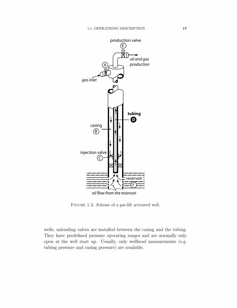
1.1. OPERATIONS DESCRIPTION 17
E
production valve
gas inlet
oil and gas
productionA
B
C
injection valve
casing
D
tubing
oil flow from the reservoir
F
reservoir
Figure 1.2. Scheme of a gas-lift activated well.
wells, unloading valves are installed between the casing and the tubing.They have predefined pressure operating ranges and are normally onlyopen at the well start up. Usually, only wellhead measurements (e.g.tubing pressure and casing pressure) are available.
18 CHAPTER 1. PROCESS DESCRIPTION AND PROBLEMATIC
1.2. Operating conditions and efficiency
Here, we explain the selection rules that define the optimal gas-lift op-erating conditions for a single generic well. Then we show that numerousinterconnexions between wells prevent them from being operated at theiroptimal conditions. Moreover field operations are all the more difficultthat solving this highly coupled optimal problem is not the only issue,preventing wells from being unstable has also to be addressed.
1.2.1. Normal operating conditions. — At the single well scale, themain idea is to derive from Bernoulli’s law the response curve, a staticequation giving the oil production with respect to the gas injection flowrate. Defining a linear cost function depending on oil price and gas costlet us compute the optimal gas-lift injection. At the multi-well scale,we give some insights of the constraints arising from the interconnexionsbetween wells.
1.2.1.1. At the single well scale. — Given a particular gas-lifted welland a hardware configuration, one can set-up the production rate byacting upon two parameters (inputs), u the production choke openingand qgi the gas injection rate. We now detail the impact of those twoparameters on the production. A nomenclature is given in Table 1. Anatural objective is to maximize the oil production while minimizing theneed of gas.
1.2.1.1.1. Gas injection impact. — To study the effect of a gas injectionrate variation, we assume that the production choke opening is constant.From the Bernoulli equation, one can derive that the pressure gradientin the tubing has a steady state value
pr − ps = ∆pdrawdown + ∆pchoke + ∆pgravity + ∆pfriction(1)
Parameters ∆pdrawdown, ∆pchoke, ∆pgravity and ∆pfriction represent pres-sure gradients in the tubing due to the draw down, the production choke,gravity and friction respectively. These four terms depend on qgi and qlp(the injected gas flow rate and the produced liquid flow rate respectively).Therefore, from equation (1), qlp one can predict the amount of oil pro-duced for a given gas injection rate qgi. When gas injection is low, thetwo dominant terms are ∆pdrawdown and ∆pgravity . Then, equation (1)
1.2. OPERATING CONDITIONS AND EFFICIENCY 19
reduces to
pr − ps = ∆pdrawdown(qlp) + ∆pgravity(qlp, qgi)
where pr and ps are the reservoir pressure and the well downstream pres-sure, respectively. By the implicit function theorem, this defines φ suchthat qlp = φ(qgi), and we have
φ′(qgi) = − ∂gi∆pgravity
∂lp∆pdrawdown + ∂lp∆pgravity
with the obvious notations ∂gi = ∂∂qgi
and ∂lp = ∂∂qlp
. The pressure
gradient due to gravity effect (∆pgravity) decreases with the gas injectionrate and increases with the liquid flow rate. The pressure gradient in thedraw-down zone (∆pdrawdown) increases with the liquid flow rate from thereservoir. Therefore, for low amount of gas injection rate
φ′ > 0
When large gas injection rate are considered the two predominantterms in equation (1) are ∆pdrawdown and ∆pfriction. Then equation (1)reduces to
pr − ps = ∆pdrawdown(qlp) + ∆pfriction(qlp, qgi)
One finds
φ′(qgi) = − ∂gi∆pfriction
∂lp∆pdrawdown + ∂lp∆pfriction< 0
since, under these conditions, the pressure gradient due to frictions effectsincreases with the gas injection rate and with the liquid flow rate
In summary, at low gas flow rate, injecting more gas tends to raise theliquid production, but at high flow rate, it decreases it. In between thesetwo regions there is a (possibly non unique, though unique in practice)gas-lift optimal point where φ′ = 0.
1.2.1.1.2. Choking impact. — In a first approximation, it is usually as-sumed that choking mainly affects the pressure gradient in the produc-tion choke. Denoting u the choke opening and assuming qgi constant, wedefine ψ such that qlp = ψ(u). From equation (1), one finds that
ψ′(u) = − ∂u∆pchoke
∂lp∆pgravity + ∂lp∆pdrawdown + ∂lp∆pfriction + ∂lp∆pchoke
> 0

20 CHAPTER 1. PROCESS DESCRIPTION AND PROBLEMATIC
0 50 100 150 200 2500
50
100
150
200
250
300
350
400
450
Qgi [kSm3/d]Qoptgi
Qlp
[m3/d]
Figure 1.3. Performance curve (liquid production Qlp with re-
spect to gas injection flow rate Qgi) derived from OLGAr2000
simulations (numerical set up given in Appendix A, Table 1).
The black star shows the optimum gas-lift injection Qoptgi for
given economic conditions.
since all pressure gradients increase with the liquid flow rate, and becausethe gradient in the production choke decreases with the opening u.
Therefore, wells ought to be operated at maximum production chokeopening.
1.2.1.1.3. Performance curve and economic considerations. — Thanksto the formulas presented in the two previous paragraphs one can getan idea of the shape of a typical performance curve, i.e. the functionexpressing the oil production with respect to the gas injection rate and tothe production choke opening. More detailed computations can be foundin [11], where different methods based on the energy balance equationare given such as the more widely accepted procedure by Poettman andCarpenter.
1.2. OPERATING CONDITIONS AND EFFICIENCY 21
Figure 1.3 shows a typical performance curve derived fromOLGAr2000 simulations. OLGAr2000 is a Transient Multiphase FlowSimulator. A realistic dynamic oil-gas model is used along with semi-implicit numerical solver (see [32] for details). A complete numericalset-up is given in Appendix A, Table 1. This curve possesses a gas injec-tion for which the liquid production reaches an optimum. Assuming thatan infinite amount of gas is available, the optimal gas injection can bedefined as follows. It correspond to the operating point at which injectingmore or less gas will lead to less profit. Profit is defined as the price ofoil times the oil produced minus the price of gas times the amount of gasused. Therefore, optimal gas injection is the one at which the derivativeof the performance curve equals the cost of the used gas divided by theproduction profit. Usually, it is slightly less than the point cancelling thederivative of the performance curve.
1.2.1.2. At the multi-well scale. — We have been focusing on singlewells. Yet, one also has to take into account constraints that arise fromthe coupling between the wells. A single well sees the rest of its networksthrough the following parameters (see Figure 1.4 for a complete view ofthe system)
– the gas availability,– the pressure of the gas network,– the pressure of the reservoir,– the pressure downstream the production choke.
In facts, each of the three pressures correspond to a separate network.The amount of gas available is upper bounded by the number and thecapacities of compressors on the network. The pressure at the upstreamof the production choke must match the surface equipments constraints(e.g. it must be higher than a defined limit allowing the flow in theexport pipe).
Bottom hole pressure variations create a local gradient in the reservoirthat propagates in a way depending on the physical properties of thegeological formation. Presence of faults, change of porosity and/or per-meability create convoluted transient gradients that affect the reservoirpressure at the bottom of the neighbor wells.

22 CHAPTER 1. PROCESS DESCRIPTION AND PROBLEMATIC
gas network
production network
compressor separator
reservoir
reservoir
Figure 1.4. Schematic of an onshore installation. Wells are
linked together through three networks: the gas network, the
production network and the reservoir
Well production is globally optimized on the basis of technical con-straints and economical and strategic objectives. Constraints such assafety, production rules, reservoir extraction policy (maximum flow rateper well, production quotas etc...), well-bore formation interface and ca-pacity have to be taken into account. The optimal operating points fora set of wells is often different from the set of optimal operating pointsfor each well. In practice, these constraints are handled by a team ofengineers based on geophysical parameter computations.
1.2.2. Unstable operations conditions and their cost. — As wehave seen it, finding optimal operating points can imply numerous con-straints. Yet, a very important problem is usually forgotten and underestimated. Wells are often not at steady state. They are often locked inoscillating modes, called headings, which correspond to regular and/orirregular changes in flow parameters (pressures and fluid rates) occurringin the system. Figure 1.5 shows an on-site example of well instabilities.

1.2. OPERATING CONDITIONS AND EFFICIENCY 23
0 2 4 6 8 100
0.5
1
0 2 4 6 8 100
0.5
1
0 2 4 6 8 100
0.5
1
pt(0
)T
t(0
)q l
s
Time
Figure 1.5. Well instabilities example. Wellhead pressure,
temperature and oil flow from the separator are represented.
An almost periodic regime appears while oil production is inter-
mittent. Scales are omitted for confidentiality reasons (courtesy
of TOTAL).
There is a slug production as can be seen on the oil flow from the separa-tor (the oil flowing from the well could not measured). The phenomenonseems periodic even though any absolutely repeated pattern cannot beclearly seen.
1.2.2.1. At single well scale. — The average amount of oil produced inunstable conditions is much lower than predicted.
Finally, let us recall that operating in unstable conditions sharply in-creases the risk of severe reservoir damage and troubles in the draw-downzone.
1.2.2.2. Instabilities propagation. — As described in Section 1.2.1.2 awell is part of a highly coupled system of wells, surface installations and

24 CHAPTER 1. PROCESS DESCRIPTION AND PROBLEMATIC
reservoirs linked by a network of pipes. In particular, each time a wellbecomes unstable, there is a risk for the other wells to be contaminated.In normal situations, because the pressure of the separator is often con-trolled, the slugs can be absorbed and do not lead to changes of thedownstream pressures of the other wells. Yet, these margins are verythin and if the pressure in the export pipe (see Figure ??) is close tothe separator pressure, a decentralized controllers structure is not ableto cope with the change of flow inlet. The separator pressure sharplyincreases which, in turn, destabilizes the other wells. To overcome this,predefined safety rules (e.g. to shut down a well when its downstreampressure is above a certain constant) are used. Keeping a majority ofwells quite stable is often preferred to producing from all wells. This nonoptimal strategy is very frequent in practice.
Similarly, wellhead casing variations should not propagate upstreamin the gas network because gas flow controller aims at guaranteing aconstant gas injection however the upstream or downstream pressuresmay vary. Yet, if the upstream pressure in the gas network is close tothe wellhead pressure in the casing, the gas control valve cannot absorbthe oscillations anymore.
Finally, the reservoir can also be seen as a network through whichinstabilities (cyclic changes of pressure and flow rates) can propagate.This last point should not be overlooked.
In summary, instabilities have a very high cost. Not only do they lowera single well productivity, but also they propagate and cause shut downs,safety alarms trigger, compressor failures and eventually negatively im-pact on the productivity of the whole field.

CHAPTER 2
A DYNAMICAL SYSTEM APPROACH
TO THE STUDY OF INSTABILITIES
UNE APPROCHE DYNAMIQUE DEL’ANALYSE DES INSTABILITÉS
Dans ce chapitre nous présentons notre contribution principale : lamodélisation et l’analyse de la stabilité des deux instabilités les plusrépandus pour les puits activés en gas-lift. Dans un premier temps nousnous intéressons à l’instabilité la plus référencée dans la littérature : lecasing-heading. Dans la Section 2.1 nous décrivons ce phénomène et nousen expliquons le mécanisme. Grâce à une réduction du modèle présentépar [3] nous montrons que le casing-heading peut être intreprêté comme lecycle limite d’un modèle à deux dimensions. Nous en donnons une preuvemathématique en nous plaçant dans un cadre relativement général nonLipschitz. En résumé, le casing-heading apparaît résulter du couplageentre les deux parties qui composent le puits.
Une idée simple pour éradiquer ce phénomène pourrait être de faire ensorte que les deux parties du puits se comportent de façon indépendantes.Un tel découplage est techniquement réalisable. Malheureusement, dansle système ainsi découplé il peut apparaître un autre type d’instabilité : ladensity-wave. Ce phénomène résulte de la propagation d’une successionde bouchons liquides et de bulles de gaz dans le puits. Son étude néces-site une modélisation spécifique sous la forme d’un modèle à paramètresdistribués, que nous présentons dans la Section 2.2. L’analyse de la sta-bilité de ce système dynamique nous permet d’interpréter la density-wavecomme une bifurcation.
Le puits peut donc être modélisé par la combinaison des modèlesprésentés aux Sections 2.1 et 2.2. Il est l’interconnexion d’un modèleà paramètres distribués avec un système dynamique du premier ordre.

26 CHAPTER 2. A DYN. SYS. APPR. TO THE STUDY OF INSTABILITIES
La stabilité est alors étudiée dans la Section 2.3 grâce au théorème despetits gains. Nous nous intéressons particulièrement à l’évolution ducomportement du puits lorsque certains paramètres évoluent. Les résul-tats obtenus sont en accord avec les règles utilisées généralement sur site(et vont d’ailleurs au-delà).
In this chapter lies our main contribution: the modeling and the stabil-ity analysis of the two main unstable phenomena occurring on gas-liftedwells. In Section 2.1, we focus on the so-called casing-heading instability.This is the best-know unstable mechanism. We give a reduction of themodel proposed in [3] in order to analyse the casing-heading as a limit cy-cle of a two-dimensional model with switches. In Section 2.2, we describethe density-wave instability. The propagation in tubing is modeled as adistributed parameters model, which let us analyse its stability. At last,in Section 2.3, we propose a complete model for the well as the connexionof a stable first order model (the casing) and a distributed parametersmodel (the tubing). Stability analysis is performed thanks to the smallgain theorem. Well known operating rules are shown to be in accordancewith the stability properties of the model.
2.1. The casing-heading instability
In this first section, we focus on the best-known and best understoodof the unstable phenomena: the casing-heading instability. [9] lists threetypes of headings that can be encountered. They are classified accordingto where the free gas cyclically builds up and discharges: tubing head-ing, formation heading and casing heading. This location-dependent ter-minology tends to be replaced by a terminology where instabilities aredescribed by classes of mechanisms. Casing heading is the only one thathas kept is name, because not only has it been described for a long timebut its mechanism has also been understood in details.
In this section, we first describe this phenomenon, then we recall thefinite-dimensional modeling of [24]. Thanks to this model, we derive a

2.1. THE CASING-HEADING INSTABILITY 27
complete description of the known oscillating mode under the form of alimit cycle of a 2D model with switches. Mathematical proof is givenwith relatively few hypotheses on the model properties. This stresseswhat, in the physical structure of the well, leads to the casing-headingphenomenon.
2.1.1. Casing-heading description. — This cyclic phenomenon hasbeen described in many publications such as [43], [42] and [26]. Orig-inally, its sequence was divided into 4 phases in [43] and in seven in[26]. Figure 2.2 shows an example of casing-headings obtained withthe OLGAr2000 simulator. We choose to describe casing-heading as afour stages phenomenon (shown in Figure 2.2). One should report toFigure 2.1 for an illustration of the terms involved in the following de-scription, notations are given in Appendix B, Table 1.
1. Starting with a downhole annulus pressure that is lower than thebottom-hole pressure, there is no gas flow through the gas injection
valve into the tubing. As the gas flow rate at the surface is keptconstant the pressure in the casing builds up.
2. After some time, the annulus pressure exceeds the downstream pres-sure in the tubing. Gas is injected into the tubing. The injectedgas lowers the tubing gradient. The bottom-hole pressure beginsto decrease. Simultaneously, the production rate and the wellhead
tubing pressure begin to increase.3. Gas now flows from the annulus into the tubing at an increasing
rate. Because insufficient gas can be supplied, the pressure in thecasing sharply decreases. Oil and gas are produced through theproduction choke at a high rate. Wellhead tubing pressure reachesa maximum and the bottom-hole pressure reaches its minimum.
4. With decreasing annulus pressure, the gas flow rate entering thetubing drops. Therefore, the gradient in the tubing gets heavier, andthe bottom-hole pressure starts to increase again. The productionrate and the wellhead pressure decrease again. The bottom-holepressure equals the annulus pressure, the gas injection in the tubingstops. The whole system reaches Phase 1 of the description

28 CHAPTER 2. A DYN. SYS. APPR. TO THE STUDY OF INSTABILITIES
hproduction valve
gas inlet
oil and gas
production
injection valve
casing/annulus
tubing
oil flow from the reservoir
well head
bottom hole/down hole
reservoir draw down zone
0
H
L
z
Figure 2.1. Schematic of the well. Zones of consideration
(well head zone, bottom hole zone) appear in gray.
2.1.2. Modeling. — Different types of models have been developedto represent this instability. For example in [43], a complete and verydetailed model is presented. It not only takes into account the one di-mensional propagation in the production pipe, but also the shape of thebubble of gas entering the tubing and the liquid film fall-back. Theresults of this very precise modeling are compared with measurementsobtained from a laboratory-scaled experiments. The aim of such a finemathematical description is to predict the well behavior so that optimaloperations set point can be designed. Such an approach relies on the idea

2.1. THE CASING-HEADING INSTABILITY 29
0 100 200 300 400 500 60020
22
24
0 100 200 300 400 500 600
110
120
130
140
0 100 200 300 400 500 600
120
140
160
1 2 3 4
[bar]
[bar]
[bar]
Injection pressure
Wellhead tubing pressure
Wellhead casing pressure
pt(L)pc(L)
(a) Pressure
0 100 200 300 400 500 6000
50
100
0 100 200 300 400 500 6000
100
200
300
0 100 200 300 400 500 6000
1000
2000
3000
1 2 3 4
qgi
qg
[kg/s]
[kg/s]
[kg/s]
Gas injection
Gas production
Liquid production
(b) Flow rate
Figure 2.2. Unstable well behavior, casing heading, obtained
with qgi = 0.2kg/s simulated with OLGAr2000 (numerical set
up given in Appendix A, 2). The four main stages of the phe-
nomenon are highlighted.

30 CHAPTER 2. A DYN. SYS. APPR. TO THE STUDY OF INSTABILITIES
that it is possible to prevent instabilities by a better design of installa-tions. Here, we aim at showing that it is possible, thanks to feedbackcontrol laws based on a better understanding of the physical mechanism,to alleviate instabilities while operating in the same conditions.
For control and mathematical analysis purposes, we seek the simplestmodel capturing the well dynamics. In [18], [19] and [3], the followingthree balance ordinary differential equations model is shown to accuratelyrepresent the casing-heading dynamics
(2)
m1 = qgi − qgm2 = qg − qgp
m3 = ql − qlpWhere m1 andm2 are the masses of gas in the casing and in the tubing,
respectively, and m3 is the mass of liquid in the tubing. Respectively,qgi, qg and qgp represent the flow rates of gas at the wellhead, into thetubing at the injection depth, and the flow rate of gas produced throughthe production choke. ql and qlp represent the flow rate of liquid comingfrom the reservoir and produced at the wellhead. All those flow rates aredescribed by the following laws
qgi = constant flow rate of gas
qg = Cg
√
ρc(L) max0, pc(L)− pt(L)qpc = Cpc
√
ρm(0) max0, pt(0)− psΨ
qgp =m2
m2 +m3qpc
qgl =m3
m2 +m3qpc
qr = PI(pr − pt(H))
Cg, Cpc and PI are constants. Ψ is the production choke opening, itranges from 0 to 1. H is the well depth and L the injection depth.Notice that the liquid flow rate from the reservoir is proportional to theterm pr − pt(0), (usually referred to as draw-down). This constant PIcharacterizes the reservoir response and stands for Productivity Index.pc(L), pt(L) represent the pressures at the injection depth on the two

2.1. THE CASING-HEADING INSTABILITY 31
pt(L)
pt(H)
pc(L)
0
H
z
L
qg
qgiqlpqgp
ql
pt(0)
ps
pc(0)
m1
m2
m3
pr
Figure 2.3. Scheme of the well and notations used in equa-
tion (2) (the casing and the tubing part have been artificially
separated to improve readability).
sides of the valve. pc(L) is the upstream pressure in the casing, andpt(L) is the downstream pressure in the tubing. ρc(L) is the gas densityin the casing at the injection depth. pt(0) is the pressure in the tubingat the wellhead and ps the pressure in the separator.
2.1.3. Stability study. — With the exception of the part locatedbetween the bottom-hole and the gas injection point which is filled with

32 CHAPTER 2. A DYN. SYS. APPR. TO THE STUDY OF INSTABILITIES
0 20 40 60 80 100 120 140 160 180 200
122124126128130132134
0 20 40 60 80 100 120 140 160 180 20020
30
40
0 20 40 60 80 100 120 140 160 180 200
100
102
104
106
108[b
ar]
[bar]
[bar]
Injection pressure
Wellhead tubing pressure
Wellhead casing pressure
pt(L)pc(L)
(a) Pressure
0 20 40 60 80 100 120 140 160 180 2000
0.5
1
0 20 40 60 80 100 120 140 160 180 2000
0.2
0.4
0.6
0.8
0 20 40 60 80 100 120 140 160 180 2000
5
10
(***)
qgi
qg
[kg/s]
[kg/s]
[kg/s]
Gas injection
Gas production
Liquid production
(b) Flow rate
Figure 2.4. Unstable well behavior, casing heading, obtained
with qgi = 0.2kg/s simulated with equation (2)
liquid, we assume that the flow in the tubing is homogeneous. Using theideal gas law and following [3], densities can be computed as follows
2.1. THE CASING-HEADING INSTABILITY 33
ρc(L) =M
RTcpc(L)
ρm(0) =m2 +m3 − ρl(H − L)St
LSt
We also get the pressure expressions from the following equations
pc(L) =
(
RTc
VcM+gLc
Vc
)
m1(3)
pt(0) =RTt
M
m2
HSt − ν0m3
(4)
pt(L) = pt(0) +g
St
(m2 +m3 − ρl(H − L)St)
pt(H) = pt(L) + ρlg(H − L)
M , R, g represent the molar mass of the gas, the ideal law constant andthe gravity respectively. St, Lc, Vc are the tubing section, the casinglength and the casing volume. The casing and tubing temperatures aredenoted Tc and Tt respectively.
Equation (4) giving pc(L) is a first order approximation of an atmo-spheric model.
Figure 2.4 shows an unstable behavior of the casing heading type sim-ulated for qgi = 0.2kg/s with equation (2). As in Figure 2.2 we see thatthere is a first phase with no injection. Then injection begins as the an-nular pressure builds up to the tubing pressure. Oil and gas are producedat the well head. At last the casing can not face the gas demand andthe annular pressure decreases. Gas injection and liquid production stop.Model (2) capture the main dynamics of the casing heading phenomenon.
This model allows us to give here some insights on the well stability(this point will be developed further in Section 2.3). Figure 2.5 and 2.6illustrate the stability. One sees that for low values of the gas injectionrate the well will be unstable. Roots crossing the imaginary axis are atbirth of this instability (see Figure 2.6).
2.1.4. Casing-heading as a limit cycle. — We now show that thecasing-heading phenomenon can be depicted as the limit cycle of a two-dimensional model with switches. This study has been published in the

34 CHAPTER 2. A DYN. SYS. APPR. TO THE STUDY OF INSTABILITIES
0 1 2 3 4 5 6 72
4
6
8
10
12
14
16
18
q l[k
g/s]
qg [kg/s]
unstable
stable
Figure 2.5. Performance curve corresponding to the
model (2) with gas injection rate qg ranging from 0.01 to 7 kg/s
and a liquid production from 3 to 17kg/s. Stable equilibrium
points are represented in green and unstable in red.
IFAC world congress in Praha (see [36]). The proof is given for a systemof the form (2) under a limited set of hypotheses on the flow rate.
Studies reveal that, around a casing-heading set-point, the system iswell modeled by a two dimensional approximation (the masses of oil andgas in the tubing are highly correlated). This representation is handy tointerpret the casing-heading oscillations as a limit cycle. Our contribu-tion is to explain the observed planar limit cycle (e.g Figure 2.2 for a sam-ple OLGAr2000 well simulation) through the Poincaré-Bendixon theo-rem. This system is related to other work on hybrid systems, such as thetwo-tank system addressed in [22], or the generalization of the Poincaré-Bendixon theorem to planar hybrid systems by [33]. Yet, several specificissues have to addressed here. The model includes two switching curves.These model the flow rate through the two valves (A and E on Figure 1.2).According to classic Saint-Venant laws (refer to [2]) the flow rate is non

2.1. THE CASING-HEADING INSTABILITY 35
-0.2 -0.15 -0.1 -0.05 0 0.05
-6
-4
-2
0
2
4
6
x 10 -3
10
20
30
40
50
60
Figure 2.6. Roots of model (2) are represented in the complex
plane for gas injection ranging from 0.01 to 7 kg/s. Color axis
goes from 0 to 100% of the gas injection range.
differentially smooth around zero. The model is thus non differentiallysmooth across the switching curves. Therefore, proving existence anduniqueness of the trajectories requires special care and does not directlyderive from a Lipschitz-continuity assumption.
2.1.4.1. Dynamics definition and hypotheses. —
Physical hypotheses. — We assume that during the casing-headingphases the oil mass is proportional to the gas mass in the tubing. There-fore, we only need two ordinary differential equations to describe thesystem. For sake of simplicity, we denote x = m1 and y = m2.
We represent the behavior of the well around an unstable set point bythe following dynamics over [x, x]× [y, y] ⊂ R
+ × R+
(5)
(
x
y
)
=
(
εqgi(x)− qg(x, y)qg(x, y)− µqgp(y)
)

36 CHAPTER 2. A DYN. SYS. APPR. TO THE STUDY OF INSTABILITIES
We note X , [x, x], Y , [y, y], X , (x, y)t and
X = F (X) = (F1(x), F2(x))T .
The positive parameters ε and µ stand for the openings of valves A and E.φ(·, X0) denote the solution of equation (5) with X0 as initial condition.
Mathematical hypotheses and physical justifications. — We assume thatboth qg and qgp vanish over their definition intervals. Let ∂F o
g and ∂F ogp
be the boundaries of the sets q−1g (0) and q−1
gp (0). We assume the followinghypotheses hold.
(H1) : qgi : R→ R is C1, strictly decreasing and does not vanish.(H2) : qg = gg τg
– τg : R2 → R, is C2, and strictly increasing w.r.t x and y.
– gg : R → R+, is C0, strictly increasing over R
+, C1 overR/0, and non Lipschitz at 0. gg(0) = 0. g′g is decreasingover R
+\0. g′g ∼ tλ with −1/2 < λ < 0.(H3) : qgp = ggp τgp
– τgp : R2 → R, is C1, strictly increasing w.r.t. y, and does not
depend on x.– ggp : R → R
+, is C0, strictly increasing over R+ and C1 over
R/0, non Lipschitz at 0. ggp(0) = 0.(H4) : τg and τgp vanish over X × Y . We define ∂F o
g , τ−1g (0) and
∂F ogp , τ−1
gp (0).
In order to construct a polygon P such as defined later on in Sec-tion 2.1.5.1, we need some further assumptions.
(H5) : ∀x ∈ X , y(x, y) < 0
(H6) : x(x, ygp) < 0
(H7) : ∀x ∈ X , τg(x, y) ≤ 0
(H8) : ∀y ∈ Y , τg(x, y) ≤ 0
where, thanks to the continuity of qgp, ygp , maxy/qgp(y) = 0.One last assumption (H9) is that a constant K, uniquely defined later
on (equation (20)) in Section 2.1.6.3 by the functions above, is not zero.
Existence conditions of a limit cycle. — Let Ω(φ) be the limit set of φ.According to the Poincaré-Bendixon theorem as expressed in [31], thefact that Ω(φ) contains no critical point combined to the uniqueness of

2.1. THE CASING-HEADING INSTABILITY 37
the solution of equation (5) is sufficient to guarantee the existence ofa limit cycle. On the other hand, exhibiting a positive invariant setcontaining no stable equilibrium implies that Ω(φ) contains no criticalpoint. Therefore we can simply check that
– there exists a positive invariant set (this is shown in Section 2.1.5),– given a particular initial condition the solution is uniquely defined
(this is addressed in Section 2.1.6).
2.1.5. Positive invariance. —
2.1.5.1. Some useful lemmas. — Let P be a polygon ((Pi)i∈[1,N ] its verte-ces) such that
(6) ∀i ∈ [1, N ], ∃λ such that−−−−→PiPi+1 = λF (Pi)
Classically, P is a positive invariant set if and only if
(7) ∀X0 ∈ ∂P, ∃t > 0 s.t. ∀ε ∈ [0, t] : φ(ε,X0) ∈ P
Lemma 1. — Assume that F is Cn on a neighborhood of X0, with X0 ∈[Pi, Pi+1]. Define u = P1×P2
‖P1×P2‖. If there exists k ∈ [1, n] s.t.
F (Pi)×djφ
dtj(0, X0) · u = 0, j = 1..k − 1
F (Pi)×dkφ
dtk(0, X0) · u > 0
then condition (7) holds.
Proof. — A sufficient condition for condition (7) to be satisfied is that−−−−→PiPi+1 ×
−−−−−−→Piφ(ε,X0) · u > 0
This is equivalent to
(8) A(ε,X0) = F (Pi)×−−−−−−−→X0φ(ε,X0) · u > 0
Since F is Cn on a neighborhood of X0, an expansion of A(·, X0) is
A(ε,X0) = εk−1(F (Pi)×dkφ
dtk(0, X0) · u+ o(1))
Therefore A(·, X0) is strictly positive and condition (7) is satisfied.
Similarly one can prove that

38 CHAPTER 2. A DYN. SYS. APPR. TO THE STUDY OF INSTABILITIES
Lemma 2. — Let X0 ∈ [Pi, Pi+1] and (j, l) ∈ (1, 2); (2, 1). Assume
that Fj(Pi) = 0. If Fl is continuous around X0 and Fj is C1, a sufficient
condition leading to (7) is
(9)
(−1)j xl(Pi)xj(X0) > 0 or
xl(Pi)xj(X0) = 0
(−1)j xl(Pi)xj(X0) > 0
Corollary 1. — If Fj(Pi) = 0 and if Fj and Fl are only C0, a more
restrictive condition is
(−1)jxl(Pi)xj(X0) > 0
2.1.5.2. Positive invariant set candidate. — Two curves play a key rolein the construction of the candidate rectangle P = (P1P2P3P4). Theseare the set (x, y)/ x = 0 and the set (x, y)/ y = 0. We show thatthis rectangle, which is illustrated in Figure 2.7, satisfies equation (6).
Construction of P1, P2 and P3. — Let ψ be defined by
ψ(x) , εqgi(x)− qg(x, ygp)
From (H6) and (H8), ψ(x) > 0 and ψ(x) < 0. Since ψ is continuous,increasing, we can uniquely define
x1 = maxx/ψ(x) = 0
We note P1 , (x1, ygp). At that point, both x and qgp vanish. Further,similar arguments relying on (H5), and (H2)-(H8) respectively, uniquelydefine P2 , (x1, y2) with y2 , miny/y(x1, y) = 0 and P3 , (x3, y2)
with x3 , maxx/x(x, y2) = 0.Construction of P4. — Let P4 , (x3, ygp). [P3, P4] is tangent to the fieldat P3. Further, [P4, P1] is tangent to the field at P4. This arises fromthe following argument. Since qg is cancelling at (x, ygp) and strictlypositive at P1, we can choose ε parameter in equation (5) such that[P4, P1] ∩ ∂F o
g 6= ∅. Therefore qg(P4) = 0. As a consequence, x(P4) >
0 and y(P4) = 0.

2.1. THE CASING-HEADING INSTABILITY 39
2.1.5.3. Intersections with switching lines. — Let X2g , (xg, ygp) with
xg = maxx/(x, ygp) ∈ [P4, P1] ∩ ∂F og . Remembering that qg(P3) =
εqgi(P3) > 0, we conclude [P3, P4] ∩ ∂F og 6= ∅. We note X1
g , (x3, yg)
with yg , maxy/(x3, y) ∈ [P3, P4] ∩ ∂F og .
2.1.5.4. Positive invariance. — Let X0 be a point on the side of therectangle. We want to prove that the trajectory φ(·, X0) = (φx, φy)
t
starting at X0 remains inside P for t > 0. We assume that trajectoriesare uniquely defined, this is proven at Section 2.1.6.
Using Lemma 2 at points where F2 is not C1. — Let X0 ∈ [P1, P2].F1 vanishes at P1, so F1 being C1 and F2 only continuous around X0
will complete the list of hypotheses needed to apply Lemma 2. F2 iscontinuous by definition and F1 is C1, because ∀X0 ∈ [P1, P2]
qg(X0) ≤ qg(P1) = εqgi(P1) > 0
Therefore, checking condition (9) of Lemma 2 will prove that the trajec-tory starting at X0 goes inside (P). If X0 ∈]P1, P2] the condition rewrites−y(P1)x(X0) > 0. As −qg is decreasing w.r.t. y, x(X0) < 0. Addingthat y(P1) > 0 ensures that the condition holds. If X0 = P1 the condi-tion rewrites −y(P1)x(X0) > 0. As x(X0) = −∂yqg(X0)y(X0) < 0 thiscondition holds. Following along the same lines it is easy to check thatLemma 2 can be applied at every point of ∂P except X1
g and [P4, P1].At these points the C1 condition is not verified. Notice also that at eachvertex two conditions have to be verified, one for each side.
Using Corollary 1 at points where F1 and F2 are only C0. — When X0
is an element of X1g∪]X2
g , P1] none of F coordinates vanish, therefore wecan simply use the fact that F is continuous to apply Corollary 1. So forX0 = X1
g the condition is −x2(P3)x1(X0) > 0 which is easily checked. AtX0 ∈]X2
g , P1] the condition is x1(P4)x2(X0) > 0.
A proof by contradiction when X0 ∈ [P4, X2g ]. — Neither Lemma 2 (F2
is not C1) nor Corollary 1 (y(X0) = 0) can be used here. Yet, we canprove that a solution starting at X0 cannot go below y = ygp. Assume

40 CHAPTER 2. A DYN. SYS. APPR. TO THE STUDY OF INSTABILITIES
that there exists t2 such that φy(t2) < xgp2 , define t1 such that
(10)
∀t ∈]t1, t2], φy(t) < xgp2
φy(t1) = xgp2
Refering to the mean value theorem φy(t2) = φy(t1)+(t2− t1)φ′y(tc) with
tc ∈ [t1, t2]. φ′y(tc) = 0 implies φy(t2) = φy(t1) which contradicts (10).
Finally, as the trajectory starting at X0 ∈ ∂P satisfies condition (7), Pdefines a positive invariant set.
2.1.6. Existence and uniqueness of the trajectories. — The firsthypothesis required by the Poincaré-Bendixon theorem is the existenceand forward uniqueness of the solutions. Existence of a solution of (5)starting at X0 ∈ X × Y follows from the continuity of F . Uniqueness ofa solution of (5) starting at X0 ∈ (X ×Y)/(∂F o
g ∪∂F ogp) follows from the
differentiable continuity of F around X0.
2.1.6.1. Decoupling. — Consider X0 ∈ [P4, X2g [⊂ ∂F o
gp. qg is null atP1 and increasing with respect to x, so it cancels over [P4, X
2g ]. In a
neighborhood of any point of this segment the system is decoupled. Atthis point the system writes
x(X0) = εqgi(x0)
y(X0) = −µqgp(y0)
Both right hand sides are decreasing functions because qgp is increasingand qgi is decreasing. Thus the solution starting at X0 is unique (see[10]).
Let X0 ∈ ∂F og , such that F (X0) · ∇τg(X0) < 0. Let φ be a solution
starting at X0. F being continuous and bounded in a neighborhood ofX0, we can define T > 0 such that ∀t < T , X0φ(t) · ∇τg(X0) > 0.Therefore the solutions of (5) are the solutions of the decoupled system
x = εqgi(x)
y = −µqgp(y)
Each equation has a unique solution, so there exists a unique solutionstarting at X0.

2.1. THE CASING-HEADING INSTABILITY 41
(14)
z = ∂xτg(ξ(y, z), y)(εqgi(ξ(y, z))− gg(z)) + ∂yτg(ξ(y, z), y)(gg(z)− µqgp(y))
y = gg(z)− µqgp(y)
2.1.6.2. Transversality argument. — Let
X0 ∈ X ∈ ∂F og/F (X) · ∇τg(X) > 0 ∪ [X2
g , P1]
Rewriting dynamics (5) in the (y, z) coordinates, with z = τg(x, y), yields
(11)
z = F (ξ(y, z), y) · ∇τg(ξ(y, z), y)y = gg(z)− µqgp(y)
where ξ is a C2 function defined from the implicit function theoremapplied to z = τg(ξ(y, z), y). The decoupling argument does not holdanymore, but we can use the transversality property at 0, z is strictlypositive, therefore ∃α−, α+, T ∈ R
+\0 such that ∀t ∈ [0, T ]
(12) z0 + α−t ≤ z(t) ≤ z0 + α+t
When y0 = y and z0 6= 0, y(0) is strictly positive which allow us to defineβ−, β+, T ∈ R
+\0
(13) y0 + β−t ≤ y(t) ≤ y0 + β+t
Now, consider two distinct solutions (y1, z1) and (y2, z2), let ey , y2− y1
and ez , z2 − z1. The key of the proof is to use equation (12) to definean upper-bound to |e| = |(ey, ez)|. From (12) and (13) we deduce that∀t ∈]0, T ] y(t) > y0 and z(t) > 0. Therefore the solution of (11) startingat that point is unique. In the case of (y0, z0) = (y, 0) this property stillholds. The two solutions (y1, z1) and (y2, z2) cannot split but at t = 0.Furthermore we define T ′ such that ey, ez and their derivatives remainpositive over ]0, T ′]. The dynamics rewrites as equation (14). We replacethe C1 functions ∂xτg, ∂yτg and qgi by their first order expansion aroundX0 in the first equation of (14)
z = A−Bgg(z)− Cµqgp(y) +Dz + Ey +R(y, z)(15)
42 CHAPTER 2. A DYN. SYS. APPR. TO THE STUDY OF INSTABILITIES
With A > 0, C > 0 and
lim(y,z)→(y0,0)
R(y, z)
|(y, z)− (y0, 0)| = 0(16)
Using the mean value theorem, we can define (yc, y′c, y
′′c ) ∈ [y1, y2] and
(zc, z′c, z
′′c ) ∈ [z1, z2] such that the dynamics of e is
(17)
ey =− µw′gp(yc)ey + g′g(zc)ez
ez =(−Cµw′gp(y
′c) + E + ∂yR(y′′c , z2))ey
+ (−Bg′g(z′c) +D + ∂zR(y1, z′′c ))ez
Recalling (16) one can define T ′, k and k′ such that over ]0, T ′]
ez ≤ (−Cµw′gp(y
′c) + kE)ey + (−Bg′g(z′c) + k′D)ez
To define the upper-bound of (17), we recall the transversality argument.g′g being monotonous, we deduce
(18)
0 ≤ ey ≤g′g(z0 + α±t)ez
0 ≤ ez ≤kEey + (−Bg′g(z0 + α±t) + k′D)ez
Notice that for z0 > 0 we do not need the linear bounds of (12) to derivea proper upper-bound in (18). Yet, for z0 = 0 the upper-bound goes toinfinity, therefore we use that z(0) is not zero. Remark also that thiskind of hypothesis is not required for y. Integrating between s and t
(t < min(t′, t′′) and s > 0) gives
e(t) ≤∫ t
s
A(u)e(u)du+ e(s)
with A(t) =
(
0 g′g(z0 + α±t)
kE (−Bg′g(z0 + α±t) + k′D)
)
Using |A| =∑2
i,j=1|aij | we deduce
|e(t)| ≤∫ t
s
|A(u)||e(u)|du+ |e(s)|
Therefore, the Gronwall inequality theorem([10]) yields
|e(t)| ≤|e(s)| exp
(∫ t
s
|A(u)|du)
(19)
2.1. THE CASING-HEADING INSTABILITY 43
As the exponential term is bounded, the limit of the right-hand side ofequation (19) is also 0 when s goes to 0 which concludes the proof.
2.1.6.3. Non transverse case. — Define X0 such that X0 ∈ ∂F og and
F (X0) · ∇τg(X0) = 0. The initial conditions of equation (11) becomez(0) = z(0) = 0, y(0) < 0 and y(0) > ygp. In inequality (12), z(0) = 0
yields α± = 0. The upper-bound |A(u)| goes to infinity as u goes tozero. System (18) does not give further result. Yet, using y ∼ y0 + y(0)t,equation (15) yields
z ∼ Kt−Bgg(z)
with
K = (E − Cµw′gp(y0))(20)
The role of assumption (H9) appears here as a substitute to the transver-sality property of Section 2.1.6.2. It implies that when the field is tangentto the switching curve there exists a non vanishing higher order forcingterm (which actually arises from the coupling of the y dynamics onto thez dynamics). Using L’Hospital’s rule, we find that Kt is the predomi-nant term. Thus, for a given K, the solutions are positive or negativeexclusively. Therefore, if K < 0 we use the decoupling argument to con-clude to uniqueness. If K > 0 we use z ∼ Kt2/2 instead. As t 7→ g′g(t
2)
is integrable around 0 the exponential term of the right-hand side ofequation (19) is bounded, therefore letting s go to zero yields e(t) = 0.
2.1.6.4. Conclusion. — Away from ∂F og ∪ ∂F o
gp uniqueness follows fromthe differentiable continuity of F . Points at which the field points to-ward the τg < 0 zone were studied in Section 2.1.6.1 where a decouplingargument was used. Otherwise, when available, transversality was used(see Section 2.1.6.2). Finally, the case of a field tangential to ∂F o
g wasaddressed in Section 2.1.6.3. All cases being addressed, uniqueness isproven.
2.1.7. A case study. — While appearing as a limit case of our result(see (H2)), square roots are often used for valve modeling. Uniquenessproof follows along the exact same lines except for the final points ad-dressed in Section 2.1.6.3. Instructively, an alternative study leads to the

44 CHAPTER 2. A DYN. SYS. APPR. TO THE STUDY OF INSTABILITIES
∂Fog
∂Fogp
x = 0 y = 0
ypg
X1
g
X2
g
P1
P2P3
P4
Limit cycle
Vector field
Switching curves
Figure 2.7. Limit cycle (in blue) and positive invariant set
(rectangle P1P2P3P4) for the sample problem. Switching curves
∂Fog and ∂Fo
gp are represented.
conclusion. Let X = Y , [5/4−√
13/8, 5/4], ε = 0.1 and µ = 2. Let
qgi(x, y) ,√
2− xτg(x, y) , 13/8− (x− 5/4)2 − (y − 5/4)2
τgp(x, y) , y3
2
with gg = ggp ,√
max(0, ·). Equilibrium points are unstable with pos-itive real part complex conjugate poles. Hypotheses (H1), (H2), (H3),(H4) are verified. Let us check hypotheses (H5), (H6), (H7) and (H8)(with ygp = 0)
(H5) : ∀x ∈ X , y(x, 54) =
√
138−(
x− 54
)2 − 2(
54
)3
4 < 0
2.2. THE DENSITY WAVE INSTABILITY 45
(H6) : x(5/4, 0) = 0.1√
3/2− 1/4 < 0
(H7) : ∀x ∈ X , τg(
x, 54−√
138
)
= −(x− 54)2 ≤ 0
(H8) : ∀y ∈ Y , τg(
54−√
138, y)
= −(y − 54)2 ≤ 0
These hypotheses are also verified. Yet, α = 1/2, thus we substituteSection 2.1.6.3 with the following study. Around X0 = (y0, 0) where thefield is tangent to ∂F o
g we have, y ∼ y0 + y(0)t (y(0) < 0). Equation (15)now yields
z ∼ −B√z +Kt
With B = −1.93 and K = (E − Cµ3/4y−1/40 )y(0) = 0.503. Us-
ing L’Hospital’s rule we compute: z(t) ∼ at2, with a = 1.38. As|e(s)| = (s2), equation (16) becomes
|e(t)| ≤ (1)eb(t−s)+(2− 1−B
2√
a) ln t
s
As 2 − (1 − B)/(2√a) = 0.757, letting s go to 0 implies that e(t) = 0.
Uniqueness is proven. Figure 2.7 shows the construction of the positiveinvariant set and the limit cycle.
2.2. The Density wave instability
As predicted in Section 2.1, the casing-heading takes its origin fromthe coupling of the tubing and casing dynamics through the gas-lift in-jection. A simple idea to alleviate this phenomena is to keep the gasinjection critical, i.e. independent from the downstream pressure varia-tions. This decoupling can be achieved thanks to a hardware upgrade(new gas-lift gas design). In [42], it is advocated that such newly devel-oped gas-lift valves ensure constant gas flow rate (at constant pressure inthe casing) even when tubing pressure is only 10% less than casing pres-sure. The laterally asymmetric internal geometry of the nozzle-Venturicreates an injection valve that reaches critical flow velocity with pressuredifferential of only 10%. In [20], engineers from PDVSA report an in-teresting case study on the installation of such NOVA valves on gas-liftwells. The authors present interesting results in the case of simultane-ous variations of casing and tubing pressures. Yet, this technology doesnot address all possibly encountered cases. Cases where only significant

46 CHAPTER 2. A DYN. SYS. APPR. TO THE STUDY OF INSTABILITIES
tubing pressure variations are observed remain unsolved. In [15], some“slugging problem in Brage wells” that “is not casing heading‘” is alsoreported. This problem has not been solved by the use of Venturi-typegas-lift valve.
This underlines that, even with a constant gas-lift injection, the dy-namics of the well can be unstable. This instability cannot be predictedby the model described by equation (2). The main assumption we haveused for its derivation is though very common. It states that the pressuregradient reaches its steady state instantaneously. This is what is also im-plicitly assumed in [8], [9], [5] and [4]. Yet, this assumption preventsus from representing instabilities characterized by a fluctuation of thegas/liquid ratio in the tubing, such as the one which has been pointedout in [20] and [15]: the density-wave. In this instability, which exis-tence was first demonstrated in [23], oscillations are confined in the tub-ing while the gas injection rate is constant. Out-of-phase effects betweenthe well influx and the total pressure drop along the tubing are usuallyreported at the birth of this phenomenon. Figure 2.8 shows an exampleof a density-wave occurring on a well. This phenomenon is highly peri-odic, a repeated pattern can be clearly recognized. The observed cycleundoubtedly discards the hypothesis of casing-heading. The pressure atthe casing head is almost constant.
In this section, we propose an interpretation of the observed oscilla-tions in the tubing of gas-lifted wells. A distributed parameter modelis derived for the propagation of pressure (system (35)). It describesthe dynamics as a transport phenomenon with state dependent bound-ary condition. This equation is shown to be equivalent to a saturatedlinear delay model (equation (37)) involving the gas fraction. Analysisof the underlying characteristic equation is performed (for unsaturatedsolutions) and show that the critical parameter is the amount of injectedgas. This is consistent with state-of-the-art and suggests a simple controlstrategy which is developed in Section 3.2.
In Section 2.2.1, we detail the observed density-wave oscillating phe-nomenon. In Section 2.2.2, we derive a reference distributed delay modelfor the density propagation in the tubing. Main assumptions and theuse of Riemann invariant are explicited along with boundary conditions.

2.2. THE DENSITY WAVE INSTABILITY 47
0 0.5 1 1.5 2 2.5 3 3.50
0.5
1
0 0.5 1 1.5 2 2.5 3 3.50
0.5
1
0 0.5 1 1.5 2 2.5 3 3.50
0.5
1
pc(0
)p
t(0
)Q
ls
Figure 2.8. Density wave occurring on a well. Casing-head
and tubing-head pressures (respectively pc(0) and pt(0)) are
represented as well as oil flow from the separator (Qls). Notice
that the casinghead pressure is almost constant, which demon-
strates that the gas injection is constant. Scales are omitted for
confidentiality reasons (courtesy of TOTAL).
In Section 2.2.3, stability analysis of the corresponding characteristicequations is performed. Comparisons with OLGAr2000 are conductedand stress the role of the amount of injected gas. This study has beenpublished in the Conference on Decision and Control, 2005, in Seville(see [39]).
2.2.1. Density-wave description. — Figure 2.9 shows an exampleof density wave instability simulated with the transient multiphase flowsimulator OLGAr2000. Typically, the depth of the well is 2500 m and thereservoir pressure is 150 bar. Oil production has an oscillating behaviorconsisting of 3 phases.
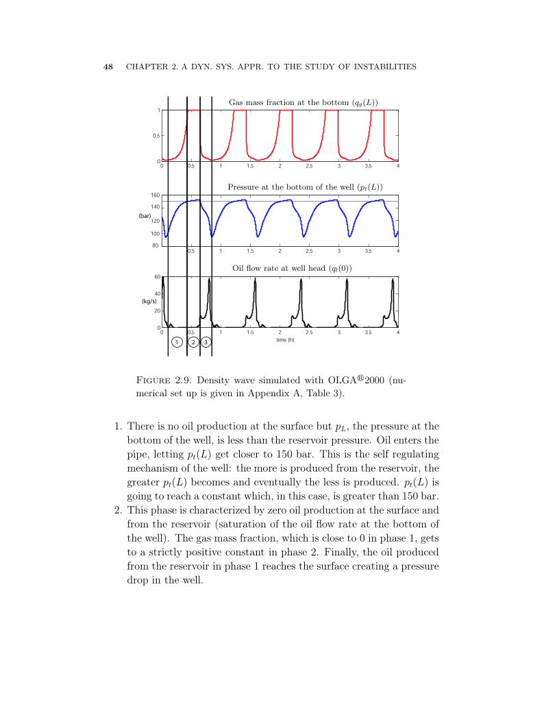
48 CHAPTER 2. A DYN. SYS. APPR. TO THE STUDY OF INSTABILITIES
0 0.5 1 1.5 2 2.5 3 3.5 40
0.5
1
0.5 1 1.5 2 2.5 3 3.5 480
100
120
140
160
0 0.5 1 1.5 2 2.5 3 3.5 40
20
40
60
(bar)
(kg/s)
1 2 3 time (h)
Gas mass fraction at the bottom (qg(L))
Oil flow rate at well head (ql(0))
Pressure at the bottom of the well (pt(L))
Figure 2.9. Density wave simulated with OLGAr2000 (nu-
merical set up is given in Appendix A, Table 3).
1. There is no oil production at the surface but pL, the pressure at thebottom of the well, is less than the reservoir pressure. Oil enters thepipe, letting pt(L) get closer to 150 bar. This is the self regulatingmechanism of the well: the more is produced from the reservoir, thegreater pt(L) becomes and eventually the less is produced. pt(L) isgoing to reach a constant which, in this case, is greater than 150 bar.
2. This phase is characterized by zero oil production at the surface andfrom the reservoir (saturation of the oil flow rate at the bottom ofthe well). The gas mass fraction, which is close to 0 in phase 1, getsto a strictly positive constant in phase 2. Finally, the oil producedfrom the reservoir in phase 1 reaches the surface creating a pressuredrop in the well.
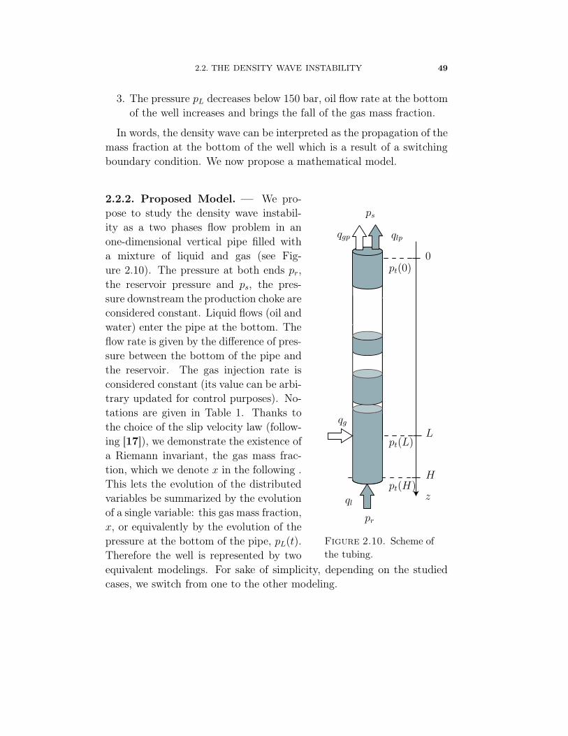
2.2. THE DENSITY WAVE INSTABILITY 49
3. The pressure pL decreases below 150 bar, oil flow rate at the bottomof the well increases and brings the fall of the gas mass fraction.
In words, the density wave can be interpreted as the propagation of themass fraction at the bottom of the well which is a result of a switchingboundary condition. We now propose a mathematical model.
pt(L)
pt(H)
0
H
z
Lqg
qlpqgp
ql
pt(0)
ps
pr
Figure 2.10. Scheme of
the tubing.
2.2.2. Proposed Model. — We pro-pose to study the density wave instabil-ity as a two phases flow problem in anone-dimensional vertical pipe filled witha mixture of liquid and gas (see Fig-ure 2.10). The pressure at both ends pr,the reservoir pressure and ps, the pres-sure downstream the production choke areconsidered constant. Liquid flows (oil andwater) enter the pipe at the bottom. Theflow rate is given by the difference of pres-sure between the bottom of the pipe andthe reservoir. The gas injection rate isconsidered constant (its value can be arbi-trary updated for control purposes). No-tations are given in Table 1. Thanks tothe choice of the slip velocity law (follow-ing [17]), we demonstrate the existence ofa Riemann invariant, the gas mass frac-tion, which we denote x in the following .This lets the evolution of the distributedvariables be summarized by the evolutionof a single variable: this gas mass fraction,x, or equivalently by the evolution of thepressure at the bottom of the pipe, pL(t).Therefore the well is represented by twoequivalent modelings. For sake of simplicity, depending on the studiedcases, we switch from one to the other modeling.
50 CHAPTER 2. A DYN. SYS. APPR. TO THE STUDY OF INSTABILITIES
2.2.2.1. Physics reduction. — We first summarize the main assumptionswhich are used in the following:
(H’1) : We consider that the friction term in Bernoulli’s equation canbe neglected in comparison with the gravity term.
(H’2) : The gas velocity is assumed to be constant.(H’3) : The productivity index is assumed to be also constant, which
means that the effluents mass flow rate from the reservoir is propor-tional to the difference of pressure between the bottom of the welland the reservoir.
(H’4) : The gas volume fraction is close to the gas mass fraction.This assumption arises from the fact that in the density-wave case,at a given depth in the tubing pipe, the mixture is either composedalmost only by oil or almost only by gas.
(H’5) : The slip velocity is defined by
vg − vl =v∞rl
as in [17]. Where rl is the oil volume fraction and vg and vl the gasand oil velocities.
Pressure law. — Using Bernoulli’s law we get
p(t, z) = ps +
∫ z
0
ρm(t, ζ)gdζ(21)
In (21), using assumption (H’1), we have neglected the friction term, itis consistent with the observed low flow rates for density wave instability(see [23]). Density of the mixture is given by
1/ρm = x/ρg + (1− x)/ρl
To work with a linear expression of ρm, we use assumption (H’4) and weget that
ρm ∼ xρg + (1− x)ρl(22)
This approximation is quite false for medium values of x but since weare working with values of x close to 0 or 1 this assumption is valid.Further, in the derivation of the gas density, gas is considered perfectand the temperature T is constant. Besides, we assume that the pressuregradient between the injection point and the wellhead is constant and

2.2. THE DENSITY WAVE INSTABILITY 51
computed from boundary condition. Notice that pt(·, H) = pt(·, L) +
ρlg(H − L). Therefore, we denote pr = pr − ρlg(H − L) the appearingreservoir pressure. The pressure gradient is thus assumed to be equalto pr−ps
L. Simulations have shown that this simplification improves the
numerical tractability while saving the oscillatory behavior. Using theexpressions in (22) and after substitution in (21), we get
p(t, z) = ps + ρlgz +
∫ z
0
x(t, ζ)g
(
(L− ζ)ps + ζpr
LRTt− ρl
)
dζ(23)
Slip velocity and Riemann invariant. — We use assumption (H’5) todefine the slip velocity law. Mass conservation laws write
∂ρgrg
∂t+∂Φg
∂z= 0(24)
∂ρlrl
∂t+∂Φl
∂z= 0(25)
where Φg and Φl are respectively the gas and oil mass flux and rg the gasvolume fraction. Since
x =rgρg
rgρg + rlρl(26)
one can combine (24), (25) and (26), to obtain
∂x
∂t+ vg
∂x
∂z= 0
This proves that x is a Riemann invariant (see [13]). For sake of simplic-ity we use assumption (H’2) and assume that vg is constant. On real wellsit is not as simple and we shall discuss the implications of this hypothesisin Section 3.2.1.3. This implies
x(t, z) = x
(
t− L− zvg
, L
)
= xL
(
t− L− zvg
)
Therefore, knowing bottom well gas mass fraction t 7→ xL(t), we getthe profile (t, z) 7→ x(t, z) in the tubing. Replacing this expression inequation (23) and denoting pL(t) = P (t, L), we find
p(t, L) = p?L +
∫ t
t−δ
k(t− ζ)xL(ζ)dζ(27)

52 CHAPTER 2. A DYN. SYS. APPR. TO THE STUDY OF INSTABILITIES
with
δ = L/vg(28)
p?L = ps + ρlgL(29)
and
[0, δ] 3 t 7→ k(t) , Vgg
(
tps + (δ − t)pr
δRTt− ρl
)
< 0(30)
Notice that k is a strictly decreasing affine function.
Boundary condition. — Classically, (see [11]), the oil rate ql is givenat the reservoir boundary by the constant Productivity Index (PI, seeassumption (H’3)) through
ql(t, H) =PImax(pr − pt(t, H), 0)(31)
=PImax(pr − pt(t, L), 0)
By definition,
xL(t) =1
1 + PI/qg max(pr − pL(t), 0)(32)
We want to simplify this last expression in the case of large PI. Onone hand, as pr − pt(L) begins to be positive, xL goes to zero. Let βdenote a threshold parameter. In particular xL < β is equivalent topt(L) < pr − qg
IP(1/β − 1). We denote
λ ,1
PI(1/β − 1)(33)
On the other hand, when pt(L) > pr, xL = 1. Therefore, we consider xL
as constant, equal to 1 when pL > pr and equal to 0 when pt(L) < pr−λqg.Finally, the considered expression of xL reduces to
xL = h (X) , X , 1− pr − pt(L)
λqg(34)
with
h(·) = max(min(1, ·), 0)
equation (34) is the definition we use instead of equation (32) from nowon.

2.2. THE DENSITY WAVE INSTABILITY 53
2.2.2.2. Density-wave as a distributed delay model. — We now gatherequations (27) and (34), and consider an initial condition [−δ, 0] 3 t 7→φ(t) ∈ R. The following model represents the density wave phenomenonby the evolution of the pressure at the bottom of the well pL
(35)
pt(t, L) = p?L +
∫ t
t−δ
k(t− ζ)h(
1− pr − pt(ζ, L)
λqg(ζ)
)
dζ
pt(t, L) = φ(t), t ∈ [−δ, 0]
where δ is the transport delay defined in (28), p?L, given in (29), is the
pressure at the bottom of the pipe when it is full of oil and pr is thepressure of the reservoir. k is an affine function, given in (30). It dependson the considered fluids. qg considered is one of the control variable.
2.2.2.3. Simulation results. — Figure 2.11 shows the simulations resultsof (35). When pr = 150 bar and λqg = 10 bar, we get an oscillatingtrajectory which presents similarities with Figure 2.9. Indeed, the peri-odic behavior consist of 3 phases. Alternatively, out of phase switches ofh(X(t)) and h(X(t−δ)) result in 4 slope changes of pL. These reproducethe 3 phases observed in Figure 2.9: oil production from the reservoir(zone 1), followed by a pressure buildup (zone 2), and an eventual pres-sure drop (zone 3).
2.2.2.4. Reference model for stability analysis. — Model (35) is used inSection 3.2.1.1 to design a stabilizing control law λqg. To study stabil-ity, it is equivalent (but more convenient) to consider X as defined inequation (34). It follows from (35) that
X(t) = 1− pr − p?L
λqg+
1
λqg
∫ t
t−δ
k(t− τ)h(X(ζ))dζ(36)
By derivation (assuming λqg constant), we get
λqgX(t) = k(0)h(X(t))− k(δ)h(X(t− ζ)) + k′(0)
∫ t
t−ζ
h(X(ζ))dζ
(37)

54 CHAPTER 2. A DYN. SYS. APPR. TO THE STUDY OF INSTABILITIES
0 0.5 1 1.5 2 2.5 3 3.5 40
0.5
1
0 0.5 1 1.5 2 2.5 3 3.5 4130
140
150
160
0 0.5 1 1.5 2 2.5 3 3.5 40
0.5
1
(bar)
time (h)1 2 3
PL(t)
h(X(t))
h(X(t − δ))
Figure 2.11. Density wave simulated with equation (35). The
reservoir pressure Pr is 150 bar and λqg is set at 10 bar.
We consider system (37) with an initial condition φ, defined and contin-uous over [−δ, 0], satisfying
φ(0) = 1− pr − p?L
λqg+
1
λqg
∫ 0
0−δ
k(t− ζ)h(φ(ζ))dζ
For this class of initial conditions, equations (36) and (37) have the samesolutions.
2.2.3. Stability. — We first study the stability of the trivial solutionof the following saturation-free model derived from equation (37). Wedenote
τ , δ/λqg(38)

2.2. THE DENSITY WAVE INSTABILITY 55
and C the (Banach) space of continuous function mapping the interval[−τ, 0] into R. We define xt ∈ C as
[−τ, 0] 3 θ 7→ xt(θ) = x(t+ θ)
By derivation and time scaling, equation (37) rewrites under the form
(39)
x(t) = f(xt) for t ≥ 0
x(t) = φ(t) for t ∈ [−τ, 0]
with φ ∈ C and f : C → R defined as
f(xt) =ax(t) + bx(t− τ) +c
τ
∫ t
t−τ
x(ζ)dζ(40)
with a + b + c = 0, b > 0, c < 0 and b + c > 0 (by equation (30)).Referring to the formulation used in [21], one can rewrite equation (39)as
f(xt) =
∫ 0
−τ
d(η(θ))xt(θ)(41)
with
η(θ) = (c/τ)θ, θ ∈]− τ, 0[
η(0) = a
η(−τ) = −(c+ b)
As η is continuous on ] − τ, 0[ and has bounded variation on [−τ, 0],given any φ ∈ C, there exists a unique function xt, continuous, thatsatisfies system (39). We now study stability of (39) through the solutionsof its characteristic equation. As will appear, stability depends on τ .
2.2.3.1. Characteristics equation solutions. — The characteristic equa-tion associated with (39) writes
s = a+ be−sτ +c
sτ(1− e−sτ )(42)
This equation is well defined by continuity at 0 and for all τ ≥ 0, 0 is anisolated solution. Referring to the necessary condition expressed in [40],as, for all τ ≥ 0
det(η(−τ)− η(0)) = −(a + b+ c) = 0 ≤ 0,
the trivial solution is not asymptotically stable.

56 CHAPTER 2. A DYN. SYS. APPR. TO THE STUDY OF INSTABILITIES
In the following, we characterize the location of the non zero rootswhen τ increases. In Proposition 1, we exhibit a family (τk)k∈N at whichtwo roots simultaneously hit the imaginary axis. Then, we show that, forsmall τ , roots are lying on the left half plane (Proposition 2). Further,proving that the roots cross the imaginary axis from left to right, weconclude towards the existence of τ ? > 0 (Proposition 3) such that
– for τ ∈ [0, τ ?[, all roots except 0 have strictly negative real part– for τ > τ ?, there is at least one root with strictly positive real part.
Proposition 1. — Consider the following system
x(t) = ax(t) + bx(t− τ) +c
τ
∫ t
t−τ
x(ζ)dζ(43)
with a+ b+ c = 0, b > 0, c < 0, b+ c > 0 and τ > 0. Let γ = c/b. There
exists (τk, ωk)k∈N ∈ R+ × R
+ such that, for τ = τk, besides 0 which is
always a solution, the pure imaginary roots of the characteristic equation
of (43) are ±jωk. This family (τk, ωk) is defined by
(44)
cos(ωkτk) = 1 +γσk
σk − (2 + γ)
ωk sin(ωkτk) =cσk(2 + γ)
σk − (2 + γ)
ω2k = b2(2 + γ)2
( −γ2 + γ
σk
σk − 2
)
with σk = (2b+ c)τk + 2 > 3 + γ.
Proof. — We are now looking for pure imaginary roots of equation (42).If there exists τ ≥ 0 such that jω is solution then −jω is also a solution.Therefore, we restrict our study to (τ, ω) ∈ R
+×R+\0. Equation (42)
yields
(45)
b cos(ωτ) +c
τωsin(ωτ) = b+ c
c
τωcos(ωτ)− b sin(ωτ) = ω +
c
τω
This implies
ω2 = − cτ
(2bτ + cτ + 2)(46)
2.2. THE DENSITY WAVE INSTABILITY 57
By construction, γ ∈]− 1, 0[. Note σ = (2b+ c)τ + 2 ≥ 0. Equation (45)leads to
(47) cos(
√
− γ
2 + γσ(σ − 2)) = 1 +
γσ
(σ − 2)− γ
(48) sin(
√
− γ
2 + γσ(σ − 2)) =
1
ω
cσ(2 + γ)
σ − 2− τ < 0
We derive from inequality (48) that
σ ∈⋃
k∈N
[
1 +
√
1 +2 + γ
−γ (2k + 1)2π2, 1 +
√
1 +2 + γ
−γ 4k2π2
]
Right hand side of equation (47) approaches 0 < 1 + γ < 1 as σ goesto infinity. The left hand side is oscillating thanks to the cos functionand equation (47) has an infinite number of solutions. Among these, wekeep those compatible with equation (48) and gather them in (σi)i∈N, anincreasing sequence. By construction,
limi→∞
σi = +∞
and
σi ∼i+∞
√
2 + γ
−γ 2iπ
Further, for all k ∈ N
1 +
√
1 +2 + γ
−γ (2k + 1)2π2 > 1 +√
1 + π2 > 3 + γ
The set (σi)i∈N is thus bounded by below as follows
∀k ∈ N, σk > 3 + γ(49)
This set defines a family of solutions of equation (45), (τk, ωk)k∈N usingequation (46), defined by
τk =σk − 2
2b+ c
ω2k = b2(2 + γ)2
( −γ2 + γ
σk
σk − 2
)

58 CHAPTER 2. A DYN. SYS. APPR. TO THE STUDY OF INSTABILITIES
Lemma 3. — Define s(τ) a non zero root of the characteristic equa-
tion (42). For all α > −1, β > 0 and τα > 0 there exists τ ≤ τα such
that
|s(τ)| > βτα
Proof. — By contradiction, assume that one can find (α, τα, β) (α > −1,β > 0 and τα > 0) such that for all τ ≤ τα
|s| ≤ βτα
Thus, |sτ | → 0 as τ → 0. A second order development of (42) yields
1
τ= −b− c
2+
(
b
2+c
6
)
sτ + o(sτ)
The right hand side of this development goes to −b− c/2 as τ → 0 andthe left hand side to +∞. This cannot be. Therefore, the assumption isfalse. This concludes the proof.
Lemma 4. — Define s a non zero root of the characteristic equa-
tion (42). For all τr, there exists τ ≤ τr such that
Re(s(τ)) < 0
Proof. — Assume that there exists τr such that for all τ ≤ τr
Re(s(τ)) ≥ 0
It follows that |e−sτ | ≤ 1 and that |1−e−sτ
sτ| ≤ 1. Using equation (42) we
get
|s(τ)| ≤ |a|+ |b|+ |c|which is in contradiction with Lemma 3.
Proposition 2. — There exists τ > 0 such that for all τ ≤ τ the roots
of the characteristic equation (42) that are not zero are strictly lying on
the left half plane.
Proof. — Consider a non zero root. From Proposition 1, we know that,for τ < τ1, it does not intersect the imaginary axis. Further, we know,from Lemma 4, that there exists τ < τ1 such that the root lies on the lefthalf plane. Since the real part of the root is continuous with respect to τ(by the implicit function theorem), the root cannot go to the right part

2.2. THE DENSITY WAVE INSTABILITY 59
without crossing the imaginary axis. This implies that, for all τ < τ1 theroot is in the left half plane. Finally, for all τ ∈ [0, τ1[, all roots except 0
have strictly negative real part. This concludes the proof.
Proposition 3. — There exists τ ∗ such that for all τ ∈ [0, τ ∗[ the char-
acteristic equation (42) has one root at 0 and all other roots strictly in
the left part of the complex plane. For all τ > τ ∗, there exists at least
one root lying strictly on the right half plane.
Proof. — Let τ be positive. As proven in Proposition 2, for small τall roots except 0 lie in the left half plane. To know whether theseroots become unstable or come back to the left hand side, we computeRe ∂s
∂τ |±jωk. We use equations (44) and after some computations we get
∂s
∂τ |s=jω=
−bω2e−jωτ + cτ2 (1− e−jωτ )− cjω
τe−jωτ
−2jω − b− c+ be−jωτ − bjωτe−jωτ + ce−jωτ
and
Re∂s
∂τ |±jωk
= − γb2(2 + γ)3(σk − 3− γ)(σ2
k + (2γ2 − 2 + 5γ)σk − 2γ(3 + γ)2)(σk − 2)
From (49) and noticing that σ2k + (2γ2 − 2 + 5γ)σk − 2γ(3 + γ)2 > 0 for
σk > 2, we have
Re∂s
∂τ |±jωk
> 0
Therefore, after crossing the imaginary axis the roots always go to theright half plane. Thus simply, τ ∗ = τ1 = σ1−2
2b+c.
2.2.3.2. Conclusion. — Parameter τ has a direct impact on the rootslocation of the characteristic equation. Increasing the time delay τ orletting the roots be unstable are equivalent. Recalling τ = δ
λqg, this
last remark means that there exists a minimal gas injection rate thatguarantees stability of the roots. Study of the characteristic equation is akey to the interpretation of the observed oscillating behavior. Dependingon λqg trajectories of model (37) behave as follows. Unstable solutionsof the model (37), which, initially match with unstable solutions of alinear system of type (40), finally reach saturation yielding behaviorsdepicted in Figure 2.11. Stable solutions remain bounded and if the

60 CHAPTER 2. A DYN. SYS. APPR. TO THE STUDY OF INSTABILITIES
initial condition is well chosen (e.g. constant) they do not reach thesaturation.
2.2.4. Physical interpretation: the role of the gas expansion.— We now give some physical insights on equation (40). The threeparameters of this equation are closely related with the difference ofgas and oil density between the top and the bottom of the well. Moreprecisely, we demonstrate that without the gas density gradient in thetubing, i.e. the gas expansion, the density wave would not exist.
Coefficients a, b and c of the characteristic equation (42) express interm of physical parameters. Recalling (30),
a = k(0) = vgg
(
pr
RTt− ρl
)
b = −k(δ) = vgg
(
ρl −ps
RTt
)
c = δk′(0) = vgg
(
ps
RTt
− pr
RTt
)
We notice that the key parameters of equation (42) all are proportionalto difference of densities. This implies, from the analysis presented inSection 2.2.3 that stability depends on difference of densities between oiland gas and on the gas expansion.
We now show the key role played by the gas expansion term. Let uscompletely ignore it. This means that ρg(0) ∼ ρg(H) or equivalently thata = b and c = 0. In these circumstances, the dynamics of the gas massfraction at the bottom of the well is described by
x(t) = x0 − a∫ t
t−τ
h(x(θ))dθ(50)
Where a, x0 and τ are strictly positive real numbers.
Change of variable. — A change of variable yields (t← at, τ ← aτ andx(t)← x(t/a).
x(t) = x0 −∫ t
t−τ
h(x(θ))dθ(51)
Following [21], it is possible to rewrite this equation under the form

2.2. THE DENSITY WAVE INSTABILITY 61
(52)
x(t) = −h(x(t)) + h(x(t− τ))x(t) = φ(t) for t ∈ [−τ, 0]
provided
φ(0) +
∫ 0
−τ
h(φ(θ))dθ = x0
Let us note xt: [−τ, 0] 3 0 7→ xt(θ) = x(t+ θ) ∈ R and
f(xt) , −h(x(t)) + h(x(t− τ))(53)
We now study the properties of solutions of equation (52).
Existence and uniqueness of solutions. — Let us show that f is a Lips-chitz function. We define the following norm over the set of continuousfunctions mapping φ [−τ, 0] 7→ R
‖φ‖ =
∫ 0
−τ
|φ(θ)|dθ + |φ(0)|+ |φ(−τ)|(54)
Since h is a Lipschitz function (its Lipschitz constant equals one), wededuce that f is also Lipschitz through the following simple calculations
‖f(xt)− f(x′t)‖ = |h(x(t))− h(x(t′))|+ |h(x(t− τ))− h(x(t′ − τ))|
+
∫ 0
−τ
|h(x(θ))− h(x(θ − τ))|dθ
≤|x(t)− x(t′)|+ |x(t− τ)− x(t′ − τ)|+∫ 0
−τ
|x(θ)− x(θ − τ)|dθ
≤‖xt − x′t‖Then, uniqueness of solutions follows from [21, 2.3]. In particular, noticethat, given φ such as φ ≥ 1, the trajectory x(t) = φ(0) is a solution.We conclude that, if the trajectory remains saturated longer than τ , itremains saturated forever.
We now show that, for any given initial condition, the trajectory con-verges to a constant equilibrium point. We first show that the trajectory

62 CHAPTER 2. A DYN. SYS. APPR. TO THE STUDY OF INSTABILITIES
is either after some times between 0 and 1 (which means that equa-tion (53) is simply linear) or, permanently, above 1 (and thus alwayssaturated). The proof consists in two cases depending on the initial con-dition. Convergence is proven by use of Lyapunov function.
We first show that if the trajectory enters the (0, 1) interval it remainsthere.
Lemma 5. — Assume that there exists a > 0 such that x(a) ∈ (0, 1),
then, for all t ≥ a, x(t) ∈ (0, 1)
Proof. — Assume that the trajectory exits (0, 1). First assume the exitpoint is 1 and consider b such that x(b) = 1 and, for all t ∈ (a, b),x(t) ∈ (0, 1).
x(t) ≤ −x(t) + 1
Then, applying Gronwall’s lemma one gets
x(t) ≤ x(a)ea−t +
∫ t
a
eθ−tdθ
So,
x(t) ≤ 1− (1− x(a))ea−t < 1
In particular for, t = b,
x(b) < 1
This contradiction shows that the trajectory can not exit the (0, 1) inter-val by passing through 1. Following along the same lines, one can showthat there does not exist b > a such that x(b) = 0.
Now, we exhibit a condition under which a trajectory, such that φ(0) ≥ 1,ends in the (0, 1) interval.
Lemma 6. — Let φ be an initial condition of equation (52) such that
φ(0) ≥ 1. There exists a such that x(a) ∈ (0, 1) if and only if∫ 0
−τ
(1− h(φ(θ))dθ > φ(0)− 1(55)

2.2. THE DENSITY WAVE INSTABILITY 63
Proof. — Assume that, for all t ∈ [0, τ ], x(t) ≥ 1. Thus h(x(t)) = 1.This assumption is consistent with φ(0) ≥ 1. Compute
x(τ) =x0 −∫ τ
0
h(x(θ))dθ
=φ(0)−∫ τ
0
h(x(θ))dθ +
∫ 0
−τ
h(φ(θ))dθ
=φ(0)−∫ 0
−τ
1− h(φ(θ))dθ
Referring to the inequality (55), we get x(τ) < 1, which prevents x
from remaining above 1 over the interval [0, τ ]. Therefore, there existst0 ∈ (0, τ ] such that x(t0) < 1. Since x is a continuous function, x(0) ≥ 1
and x(t0) < 1 imply that there exists a ∈ (0, τ ] such that x(a) ∈ (0, 1).Conversely, let us assume that inequality (55) does not hold. Then
∫ 0
−τ
(1− h(φ(θ))dθ ≤ φ(0)− 1(56)
Assume that there exists b ∈ (0, τ ] such that x(b) < 1. We have
x(b) = φ(0)−∫ b−τ
−τ
1− h(x(θ))dθ
= φ(0) +
∫ 0
b−τ
1− h(x(θ))dθ −∫ 0
−τ
1− h(φ(θ))dθ
Applying inequality (56) one gets
x(b) ≥ 1 +
∫ 0
b−τ
1− h(x(θ))dθ ≥ 1
Again, this is in contradiction with our assumption, thus, for all b ∈ (0, τ ],x(b) ≥ 1. This concludes the proof.
At last we prove that for any initial condition the trajectory convergesto an equilibrium value.
Proposition 4. — For any initial condition φ, the trajectory x of equa-
tion (53) asymptotically converges to x when t goes to +∞.
1. More precisely, if φ(0) ∈ (0, 1), then x = x0/(1 + τ)
64 CHAPTER 2. A DYN. SYS. APPR. TO THE STUDY OF INSTABILITIES
2. If φ(0) ≥ 1
(a) If∫ 0
−τ
(1− h(φ(θ))dθ ≥ φ(0)− 1
then
x = x0 − τ ≥ 1
(b) else
x =x0
1 + τ
with x0 = φ(0) +∫ 0
−τh(φ(θ))dθ
Proof. — According to Lemma 5, we know that in the (2.a) case, sincex(t) always remains greater or equal to 1 during a period at least equal toτ , the trajectory reaches a constant value x. This value can be computedthanks to the integral expression (51). One easily gets x ≥ 1.
According to Lemma 6, we know that in the (2.b) case, one can find asuch that x(a) ∈ (0, 1). This proves that, for all t > a, x(t) ∈ (0, 1).Equation (53) is autonomous, therefore we can address this case togetherwith case (1).
Assuming that φ(0) ∈ (0, 1), after some time, equation (55) reduces to
x = −x(t) + x(t− τ)Using this last form, we can show that the trajectory eventually convergestowards x = x0/(1 + τ). The proof relies on the following Lyapunovfunction candidate
V (φ) = (φ(0)− x)2 +
∫ 0
−τ
(φ(θ)− x)2dθ
Simple calculation gives
V (φ) =− 2X(X − Y ) +X2 − Y 2
=− (X − Y )2 ≤ 0
where X = φ(0) − x and Y = φ(−τ) − x. According to [21, The-orem 2.1], x is stable. To show asymptotic stability, we use LaSalle’sTheorem. We know that the trajectory eventually converges towards

2.3. GLOBAL STUDY OF UNSTABLE PHENOMENA 65
-1 0 1 2 3 4 5 6 7 8 9 100
0.5
1
1.5
τ
Figure 2.12. Case (1) : φ(0) ∈ (0, 1). The trajectory con-
verges towards a constant also comprised between 0 and 1.
the largest invariant set included in φ\V (φ) = 0, i.e. the set of con-stant trajectories. Moreover, the only constant consistent with the initialcondition φ is x. We conclude that x is asymptotically stable.
We have proven that without gas expansion the well would not sufferfrom instability. The integral term in the equation (36) is thus necessaryfor proper modeling of the density-wave.
Further studies have been done on this subject. Based on the sameLyapunov approach, [30] has derived a sufficient condition for the com-plete linearized equation (43) to be stable. This result is in accordancewith what is presented in paragraph 2.2.3. Moreover, this approach givesome insight to a possible extension to nonlinear equation (37).
2.3. Global study of unstable phenomena
In this section we finally study the well as an interconnected systemwithout neglecting neither the propagation phenomenon in the tubing (aswas done in Section 2.1) nor the buffer effect of the casing (as was donein Section 2.2). We exhibit and justify the impact of design parameters

66 CHAPTER 2. A DYN. SYS. APPR. TO THE STUDY OF INSTABILITIES
-1 0 1 2 3 4 5 6 7 8 9 100
0.5
1
1.5
τ
(a) φ(0) ≥ 1. Condition (55) is not satisfied. The
trajectory converges towards a constant greater
than 1.
-1 0 1 2 3 4 5 6 7 8 9 100
0.5
1
1.5
τ
(b) φ(0) < 1. Condition (55) is satisfied. The tra-
jectory converges towards a constant comprised be-
tween 0 and 1.
Figure 2.13. Cas 2. Depending on whether the Condi-
tion (55) is satisfied the trajectory converge betweens 0 and
1 or above 1.

2.3. GLOBAL STUDY OF UNSTABLE PHENOMENA 67
such as well depth, tubing diameter, and the role of physical parameterssuch as reservoir pressure of Productivity Index.
Understanding the implications of choices made at the design-stage inthe development of instability has concentrated a lot of research efforts.General stability criteria have been proposed. Some, such as [44], relyon steady state curves but most of the published work is based on adynamical system study.
In [6], the key assumption is that stability is guaranteed if an increaseof downhole tubing pressure causes a drop of mixture density and if thegas pipe depletes faster than the tubing pressure. Then, differential equa-tions are used to derive a criterion taking the form of a set of inequalities.A more dynamical system oriented approach can be found in [8]. Theanalysis relies on Routh’s criterion and a detailed study of the root lo-cations of a third order transfer function when physical parameters ofinterest vary. In [4], a unified criteria based on previous studies of [8]and [6] is proposed. In all these works the oil column is considered ho-mogenous, which implicitly neglects the propagation phenomenon in thetubing. These models are mainly devoted to the study of casing-headingfor which this simplifying assumption is particularly valid.
Our contribution here is to show that the well can be modeled as thefeedback connection of a distributed parameter system (the tubing con-sidered in Section 2.2) and a stable first order system (the casing as abuffer tank, considered in Section 2.1). This approach aims at encompass-ing both casing-heading and density-wave phenomena. The connectionof casing and tubing subsystems is achieved through the injection valve,which is modeled with a saturation function. This seemingly cascadedsystem contains feedback loops at two different levels. The first loopappears in the tubing itself through the gravity terms in Bernoulli’s law.The second loop takes place by means of the state dependent connect-ing term (injection valve) which serves as an input for the propagationequation. Stability of each subsystem is characterized. Additionally,input-output gains are computed and the small gain theorem allows usto conclude towards stability of the whole system when the asymptoticcondition of large amount of injected gas holds. This analysis is in accor-dance to experimental observations. It stresses the contribution of each

68 CHAPTER 2. A DYN. SYS. APPR. TO THE STUDY OF INSTABILITIES
subsystem design parameters and operating points to the stability of theglobal system.
In Section 2.3.1, we study the tubing subsystem and conclude on asufficient condition for stability. In particular, we detail the role of var-ious parameters in our proposed model and show the consistency withsome state of the art wells production knowledge. In Section 2.3.2, weconnect the casing dynamics to the tubing, and study the obtained inter-connection’s stability through the small gain theorem. We propose theinterpretation of well-known phenomena at the light of our model. Inconclusion, the density-wave phenomenon is interpreted as the stabilityloss due to the internal tubing feedback loop. Besides, the casing-headingphenomenon arises from the interconnection of the two systems.
The work in this section has appeared at the American Control Con-ference, in June 2006 under the title ”Predicting instabilities in gas-liftedwells simulation” ([38]).
2.3.1. Tubing Analysis. —
2.3.1.1. Equilibrium point and stability analysis. — Remembering thatthe parameter u in equation (35) is proportional to the gas injection flowrate in the tubing qg, one gets
(57)
pt(t, L) = p?L +
∫ δ
0
k(ζ)h
(
1− pr − p(t− ζ, L)
λqg(t− ζ)
)
dζ
Given a constant input qg, the unsaturated equilibrium pt(L) can becomputed through the integral equation (57).
pt(L) = p?L +
(
1− pr − pt(L)
λqg
)∫ τ
0
k(ζ)dζ
yielding
pt(L) =λqg
(
p?L +
∫ τ
0k(ζ)dζ
)
− pr
∫ τ
0k(ζ)dζ
λqg −∫ τ
0k(ζ)dζ
(58)
Linearization of the dynamics of (57) around the steady value of theinput and state (qg, pt(L)) yields
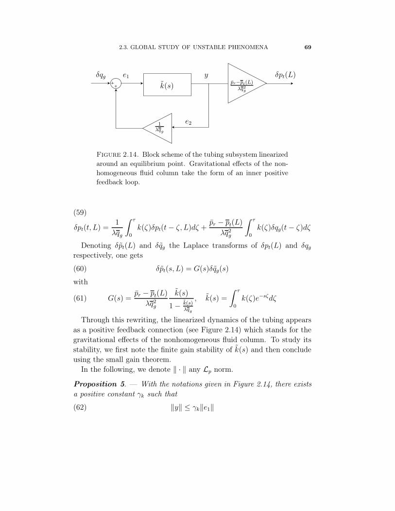
2.3. GLOBAL STUDY OF UNSTABLE PHENOMENA 69
k(s)
ypr−pt(L)
λq2g
δqg δpt(L)e1
e21λqg
Figure 2.14. Block scheme of the tubing subsystem linearized
around an equilibrium point. Gravitational effects of the non-
homogeneous fluid column take the form of an inner positive
feedback loop.
δpt(t, L) =1
λqg
∫ τ
0
k(ζ)δpt(t− ζ, L)dζ +pr − pt(L)
λq2g
∫ τ
0
k(ζ)δqg(t− ζ)dζ
(59)
Denoting δpt(L) and δqg the Laplace transforms of δpt(L) and δqgrespectively, one gets
δpt(s, L) = G(s)δqg(s)(60)
with
G(s) =pr − pt(L)
λq2g
k(s)
1− k(s)λqg
, k(s) =
∫ τ
0
k(ζ)e−sζdζ(61)
Through this rewriting, the linearized dynamics of the tubing appearsas a positive feedback connection (see Figure 2.14) which stands for thegravitational effects of the nonhomogeneous fluid column. To study itsstability, we first note the finite gain stability of k(s) and then concludeusing the small gain theorem.
In the following, we denote ‖ · ‖ any Lp norm.
Proposition 5. — With the notations given in Figure 2.14, there exists
a positive constant γk such that
‖y‖ ≤ γk‖e1‖(62)

70 CHAPTER 2. A DYN. SYS. APPR. TO THE STUDY OF INSTABILITIES
Proof. — We compute
‖k‖L1=|k1|τ 2
2+ |k2|τ < +∞
Denoting γk = ‖k‖L1and referring to [14][Lemma A.6.5] we directly
derive equation (62).
Proposition 6. — With the notations given in Figure 2.14, there exists
a positive constant qming and γ′ : [qmin
g ,+∞[3 qg 7→ R+\0, bounded and
continuous, such that
‖δpt(L)‖ ≤ γ′(qg)‖δqg‖(63)
Moreover, lim+∞ γ′ = 0.
Proof. — Recalling notations given in Figure 2.14, we get
e1(t) = δqg(t) +1
λqg
y(t)
Proposition 5 yields
‖e1‖ ≤ ‖δqg‖+1
λqg
γk‖e1‖(64)
Define qming > γk
λ. For all qg > qmin
g , we can write ‖e1‖ ≤ 11−
γkλqg
‖δqg‖ and
thus,
‖pt(L)‖ ≤ pr − pt(L)
λq2g
γk
1− γk
λqg
‖δqg‖
Finally, replacing pt(L) by its expression (58) and noting that γk =
−∫ τ
0k(ζ)dζ gives
‖pt(L)‖ ≤(∫ τ
0
−λk)
pr − pt(L)? −∫ τ
0k
(
λqg
)2 −(∫ τ
0k)2 ‖δqg‖
Therefore, we get the desired result with
γ′(qg) =
(∫ τ
0
−λk)
pr − pt(L)? −∫ τ
0k
(
λqg
)2 −(∫ τ
0k)2(65)
And lim+∞ γ′ = 0.

2.3. GLOBAL STUDY OF UNSTABLE PHENOMENA 71
2.3.1.2. Conclusion and discussion on stability of the tubing. — Clearly,the preceding derivation follows along the lines of the proof of the small-gain theorem (as exposed in [27]). If two systems are finite-gain stableand if the product of their gain is small enough (smaller than 1) thesystem resulting from their connection is also finite gain stable. Recallingthat γk derives from the integration of equation (30), here, the conditionthat guarantees stability is
γk
λqg
=Lg
RTλqg
(
RTρl −1
2(pr + ps)
)
< 1(66)
From this, we can analyze the impact of several parameters on the be-havior of the subsystem.
Increasing qg tends to lower the gain. Therefore, there exists a lowerbound on gas injection rate that guarantees stability. This is consistentwith the experimental conclusions found in [23]. These are based onOLGAr2000 simulations. In the same study, it also appears that anincrease of reservoir pressure leads to more stability. Again, from equa-tion (66), we conclude to the same result. We report in Figure 2.15, testsdone with values for pr ranging from 150 to 220 bar. At Pr = 220 bar,the system is eventually stable. We note that it is a marginal effect com-pared to an increase of the gas injection rate. This analysis providessome insights for middle to long-term aging phenomenon of reservoirswhen pressure tends to decrease with time.
Further studies reveal that a decrease of ρl or L provides more sta-bility. On the other hand, an increase of λ achieved through a decreaseof PI tends to improve stability. These parameters are known for theirstabilizing effects and can be taken into account at the design stage, e.g.to forecast instability issues.
We notice that the well-known fact that choking has a stabilizing effectis once again verified (see [16] and [23]): by increasing ps we can let thegain in (66) be smaller than 1. This is one of the key idea behind theFCW controller (see Chapter 3 for more details). In fact, choking can beused in open loop or closed loop to reach unstable points (see [37]).
Quite surprisingly, parameters such as velocity and tubing diameter donot appear in equation (66). This is due to our simplifying assumptions.In fact, both impact on stability through the definition of flow regimes,

72 CHAPTER 2. A DYN. SYS. APPR. TO THE STUDY OF INSTABILITIES
0 0.5 1 1.5 2 2.5 3 3.5 4 4.5 550
100
150
200
Pr=220Pr=180Pr=150
(bar)
time (h)
Figure 2.15. Simulation in OLGAr2000 of the impact of the
pressure reservoir on the stability of the well.
e.g. bubbly or slug flow (see [12]). We have restricted our study to a sin-gle slip velocity law. Our model does not represent changes in flow regimeand thus does not address hydrodynamic slug instability (see [12]). Thiscould be a direction of future work.
Moreover, using the small gain theorem is a conservative approach. Itdoes not provide an exact value for the turning point from stability toinstability. A closer study of the location of the roots of the characteristicequation underlying (59) is needed. Such a study is performed in [39],dealing with the impact of the gas injection rate and quantitatively show-ing that below a computable limit the roots are located in the left halfplane.
2.3.2. Stability analysis with a connected casing. — Casing andtubing, presented in Figure 1.2 are connected according to the schemein Figure 2.17. While each of these blocks can independently be stable,the resulting connected system may be unstable. Therefore, even un-der the formal assumption that guarantees the absence of density-waveinstability, casing-heading can still occur. Again, feedback connectionplays a key role. For the casing, we use a simple first order model (thefirst equation of the 3D model exposed in (2) and perform an analysis.Among several conclusions, it appears that large amounts of gas preventcasing-heading instability.

2.3. GLOBAL STUDY OF UNSTABLE PHENOMENA 73
pt(L)qg
qgi
(a) Outline
pt(L)
qgqgi
casing
(b) Block scheme
Figure 2.16. (a) Outline of the casing. (b) The inputs of the
system are the gas mass injection rate qgi and the boundary
condition pt(L) (the downhole pressure). The output is the gas
rate entering the tubing: qg.
2.3.2.1. Casing model. — A casing can be considered as an annularbuffer filled with gas from a gas network (see Figure 2.16).
Assuming that the gas is ideal and that the column is at equilibrium,we get
ρc(0) , αm1 and pc(0) , βm1(67)
where α, β are defined by
αRT =g
Sc
1
1− exp(
−gLc
RT
) = β(68)

74 CHAPTER 2. A DYN. SYS. APPR. TO THE STUDY OF INSTABILITIES
We consider as model the mass balance equation in the annulus volume
(69)
m1 = qgi − qg(m1, pt(L))
qg(m1, pt(L)) = Cg
√
αm1 max(βm1 − pt(L), 0)
2.3.2.1.1. Stability analysis and equilibrium point definition. — We as-sume normal flowing conditions, i.e. the pressure in the casing is suf-ficient to counteract pt(L) and to let the gas flow out. Given constantinput values qgi and pt(L), the equilibrium point is
m1 =1
β
(
pt(L) +
√
pt(L)2 + 4q2
gi
αβC2g
)
(70)
Linearization of equation (69) yields, for constant input qgi,
(71)
δm1 = − ∂qg∂m1
(qgi, pt(L))δm1 −∂qg
∂pt(L)(qgi, pt(L))δpt(L)
δqg =∂qg∂m1
(qgi, pt(L))δm1 +∂qg
∂pt(L)(qgi, pt(L))δpt(L)
with
∂qg∂m1
(qgi, pt(L)) =C2
gα
2qgi
√
pt(L)2 +4β
α
q2gi
C2g
(72)
∂qg∂pt(L)
(qgi, pt(L)) = −C2
gα
4βqgi
(
pt(L) +
√
pt(L)2 +4β
α
q2gi
C2g
)
(73)
Proposition 7. — For qgi > 0 the equilibrium point of (71) is exponen-
tially stable. Therefore, the linearized system (71) is finite gain stable.
One can find (γ, µ) : (R\0)2 7→ (R+\0)2, bounded and continuous,
such that
‖δqg‖ ≤ γ(qgi, pt(L))‖pt(L)‖ + µ(qgi, pt(L))(74)

2.3. GLOBAL STUDY OF UNSTABLE PHENOMENA 75
δpt(L)
δqgδqgi
tubing
casing
Figure 2.17. Block scheme of the interconnected systems lin-
earized around an equilibrium point.
These functions are
γ =C2
gα
2qgi
√
pt(L)2 +4β
α
q2gi
C2g
(75)
µ = m1(0)
√
√
√
√
C2gα
8βqgi
(
pt(L) +
√
pt(L)2 +4β
α
q2gi
C2g
)
(76)
Proof. — By assumption, the equilibrium point is such that qgi > 0, then
− ∂qg∂m1
(qgi, pt(L)) < 0
Using explicit formulas given in [27][Corollary 5.2] for linear systems, wecan write (74) with
γ(qgi, qg) = 2
∣
∣
∣
∣
∂qg∂pt(L)
(qgi, pt(L))
∣
∣
∣
∣
µ(qgi, qg) =1√2m1(0)
√
∂qg∂m1
(qgi, pt(L))
which concludes the proof.
2.3.3. Stability analysis of the connected system. —
76 CHAPTER 2. A DYN. SYS. APPR. TO THE STUDY OF INSTABILITIES
2.3.3.1. Stability criterion. — We now consider the connected linearizedsystem defined by
(77)
δm1 = − ∂qg∂m1
(qgi, pt(L))δm1 −∂qg
∂pt(L)(qgi, pt(L))δpt(L)
δqg =∂qg∂m1
(qgi, pt(L))δm1 +∂qg
∂pt(L)(qgi, pt(L))δpt(L)
δpt(L)(t) =
∫ τ
0
k(ζ)1
λqg
δpt(L)(t− ζ)dζ
+
∫ τ
0
k(ζ)pr − pt(L)
λq2g
δqg(t− ζ)dζ
In Proposition 6 and 7 respectively, we derived the gain of the tubing andcasing subsystems. Gathering and connecting these requires to matchtheir equilibrium points. This defines a constraint on pt(L) and qg. Forqgi > 0, equilibria are defined by (78). New expressions for gains throughthe connections are given in (79), (80) and (81).
(78)
qg = qgi
pt(L) =λqgi
(
pt(L)? +∫ τ
0k(ζ)dζ
)
− pr
∫ τ
0k(ζ)dζ
λqgi −∫ τ
0k(ζ)dζ
γ(qgi) = γ(qgi, pt(L))(79)
µ(qgi) = µ(qgi, pt(L))(80)
γ′(qgi) = γ′(qg)(81)
Proposition 8. — There exists a positive constant qmingi such that for
all qgi > qmingi system (77) is finite-gain stable.
Proof. — From equations (63), (74) and (79), (80) and (81) we get
‖δqg‖ ≤ γ(qgi)‖δpt(L)‖+ µ(qgi)
‖δpt(L)‖ ≤ γ′(qgi)‖δqg‖Notice that lim+∞ γ′ = 0 and lim+∞ γ > 0. Therefore, there exists qmin
gi
such that for all qgi > qmingi
γ(qgi)γ′(qgi) < 1(82)
2.3. GLOBAL STUDY OF UNSTABLE PHENOMENA 77
The small gain theorem implies that the connected system (77) is finitegain stable.
Using the fact that∫ τ
0
k(ζ)dζ = Lg
(
ps + pr
2RT− ρl
)
(83)
We compute
pt(L) =λqgi
(
ps + Lg ps+pr
2RT
)
− prLg(
ps+pr
2RT− ρl
)
λqgi − Lg(
ps+pr
2RT− ρl
)(84)
Therefore,
γ′ =
(
ps + pr
2RT− ρl
)
λLg(ps − pr + Lg ps+pr
2RT)
(λqgi)2 − (Lg)2
(
ps+pr
2RT− ρl
)2(85)
and
γ(qgi) =C2
gα
2qgi
√
pt(L)2 +4β
α
q2gi
C2g
(86)
2.3.3.2. Conclusion and discussion. — From equations (82), (85), and(86), we can analyze the influence of several parameters on the intercon-nected system. The best known effect is the role of the Cg parameter.As reported in [23], it is necessary for stability to maintain the flowthrough the injection valve critical. This is guaranteed by a choice of asmall diameter injection valve, which corresponds in our model to a smallCg. Indeed, reducing Cg lowers γ in equation (86), and thus ultimatelyguarantees inequality (82) and provides stability. Other important pa-rameters are α and β (defined in equation (67)) through which Sc, thesection of the casing, plays a key role. Increasing Sc decreases α andβ. Eventually, γ provides stability through inequality (82). In physi-cal terms, the stabilizing buffer effect is emphasized by increasing thevolume, therefore a bigger section lowers the coupling effect.

CHAPTER 3
CONTROL SOLUTIONS
SOLUTIONS DE CONTRÔLE
Les résultats du chapitre précédent ont permis de comprendre les mé-canismes d’instabilité ainsi que le rôle des paramètres physiques. Partantde ce constat, deux solutions sont envisageables. Pour éliminer les in-stabilités on peut déduire des critères de stabilité établis un protocolede définition des conditions opératoires. On peut également développerune solution de contrôle permettant de stabiliser le puits même dans desconditions a priori instables. En vue de l’application industrielle nousne considérons que la seconde solution. En effet le système physique esttrop complexe et la connaissance quantitative qu’on en a est trop ténuepour envisager de pouvoir calculer précisément des conditions opératoiresvalides. En outre il est probable que l’optimum économique se situe dansune zone instable.
Dans la Section 3.1.2.2, nous rappelons certaines solutions proposéesantérieurement dans la littérature. Elles forment deux catégories. Cer-taines proposent d’utiliser du matériel plus performant pour éviter ledéveloppement d’instabilité. D’autres utilisent une approche algorith-mique. Ces dernières modifient automatiquement les consignes desvannes d’injection de gaz et/ou de production en fonction d’indicateurs,tels que la température en tête de puits, la pression...
Nous présentons ensuite une première solution de type boucle-ouverte.Ainsi dans la Section 3.2 nous supposons que le débit de gaz injecté aufond du puits est contrôlé. Nous proposons une loi de commande dedébit, calculée à partir de la mesure de la pression de fond, qui permetde maintenir la fraction massique en gaz constante au fond du puits.

80 CHAPTER 3. CONTROL SOLUTIONS
L’efficacité de cette solution est démontrée grâce à des simulations réal-istes. Ceci souligne la pertinence du modèle à retards distribués présentésau Chapitre 2.
Nous présentons une solution plus réalistes vis à vis des contraintesopérationnelles à la Section 3.3. La faible disponibilité en gaz incite àpréférer utiliser comme commande la vanne de production. En s’inspirantde l’analyse de stabilité présentée au Chapitre 2 nous démontrons laconvergence du système bouclé avec un contrôleur de type Proportionnel-Intégral.
La loi de commande proposée utilise la mesure de la pression de fond.Ce capteur est très rarement disponible et en outre souvent sujet à despannes. Nous montrons qu’il est possible de filtrer les mesures de pres-sions en tête de casing de façon à reconstruire la pression de fond. Cettesolution est exposée à la Section 3.4 et illustrée par des résultats de sim-ulation. L’efficacité de l’observateur de pression de fond est démontréepar les résultats de son application à un puits sur un site d’exploitation.
In this chapter, we propose control solutions derived from the pro-posed modeling. First, in Section 3.1.2.2, we recall state-of-the-art con-trol techniques for gas-lifted wells. Then, we address the control problemof stabilizing the tubing subsystem. A first open-loop solution is shownto be efficient in simulation (see Section 3.2). It stresses the relevance ofthe distributed parameters model proposed in Chapter 2. More realisticcontrol solutions are addressed in Section 3.3. Following along the linesof the stability analysis of Chapter 2, we prove convergence of the closedloop system with a PI controller. At last, in Section 3.4, for sake of im-plementation, we filter measurements through an observer to reconstructunavailable variables.
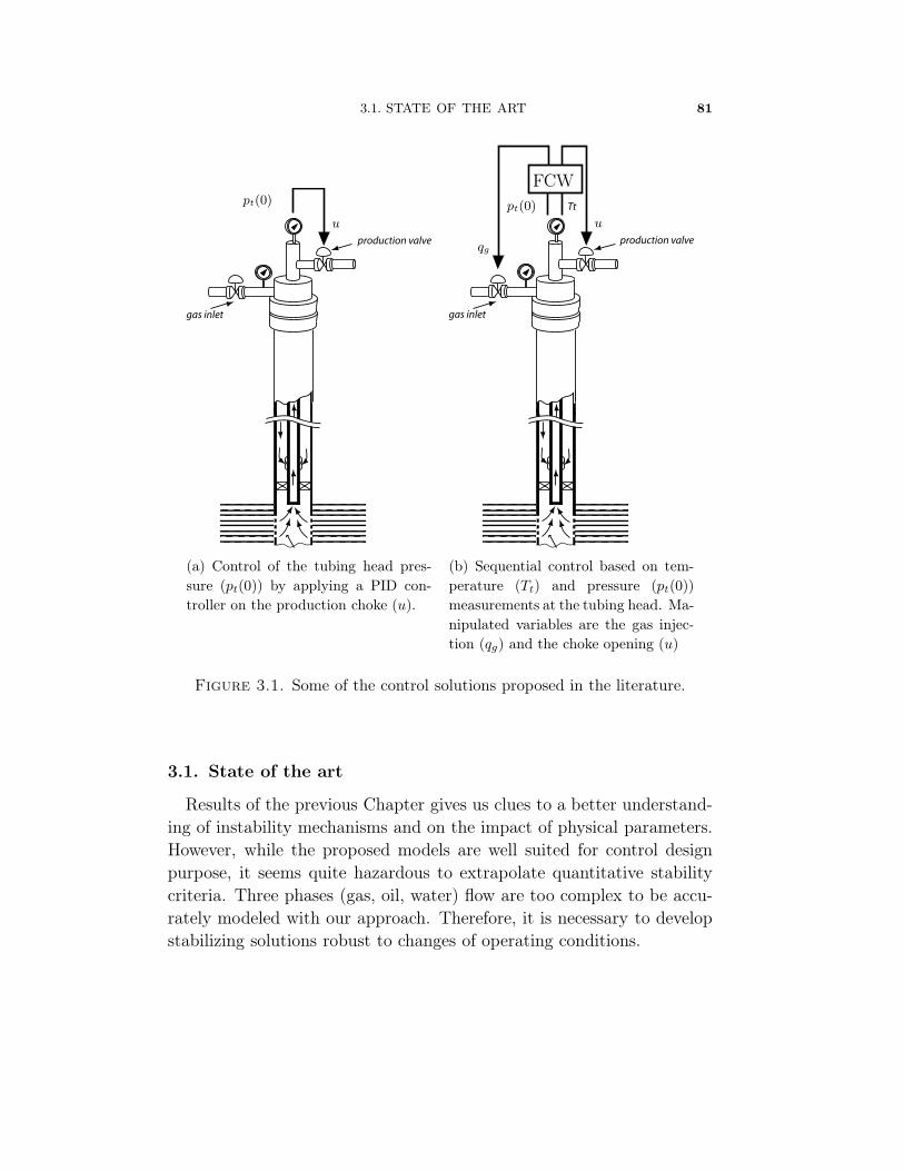
3.1. STATE OF THE ART 81
production valve
gas inlet
u
pt(0)
(a) Control of the tubing head pres-
sure (pt(0)) by applying a PID con-
troller on the production choke (u).
production valve
gas inlet
Tt
u
pt(0)
qg
FCW
(b) Sequential control based on tem-
perature (Tt) and pressure (pt(0))
measurements at the tubing head. Ma-
nipulated variables are the gas injec-
tion (qg) and the choke opening (u)
Figure 3.1. Some of the control solutions proposed in the literature.
3.1. State of the art
Results of the previous Chapter gives us clues to a better understand-ing of instability mechanisms and on the impact of physical parameters.However, while the proposed models are well suited for control designpurpose, it seems quite hazardous to extrapolate quantitative stabilitycriteria. Three phases (gas, oil, water) flow are too complex to be accu-rately modeled with our approach. Therefore, it is necessary to developstabilizing solutions robust to changes of operating conditions.
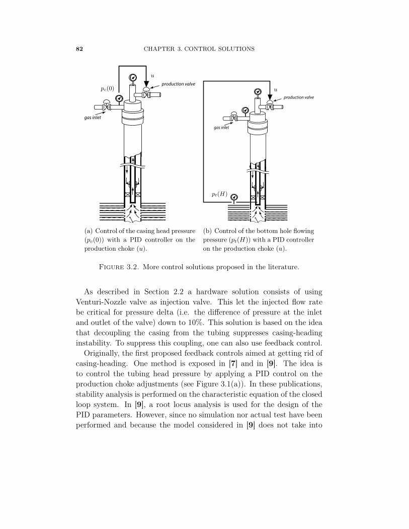
82 CHAPTER 3. CONTROL SOLUTIONS
production valve
gas inlet
u
pc(0)
(a) Control of the casing head pressure
(pc(0)) with a PID controller on the
production choke (u).
production valve
gas inlet
u
pt(H)
(b) Control of the bottom hole flowing
pressure (pt(H)) with a PID controller
on the production choke (u).
Figure 3.2. More control solutions proposed in the literature.
As described in Section 2.2 a hardware solution consists of usingVenturi-Nozzle valve as injection valve. This let the injected flow ratebe critical for pressure delta (i.e. the difference of pressure at the inletand outlet of the valve) down to 10%. This solution is based on the ideathat decoupling the casing from the tubing suppresses casing-headinginstability. To suppress this coupling, one can also use feedback control.
Originally, the first proposed feedback controls aimed at getting rid ofcasing-heading. One method is exposed in [7] and in [9]. The idea isto control the tubing head pressure by applying a PID control on theproduction choke adjustments (see Figure 3.1(a)). In these publications,stability analysis is performed on the characteristic equation of the closedloop system. In [9], a root locus analysis is used for the design of thePID parameters. However, since no simulation nor actual test have beenperformed and because the model considered in [9] does not take into

3.1. STATE OF THE ART 83
account the propagation in the tubing, it is assumed homogeneous, webelieve that more attention should be paid on other feedback methods.We now detail these approach in sections 3.1.1 and 3.1.2.
Publications [26], [15], [19] and [16] propose methods based on feed-back control using production choke opening as input and sometimes alsothe gas injection rate.
3.1.1. Steady state based feedback control. — In [26], a systemdeveloped by TOTAL, the FCW (Full Control of Wells), is presented.This system schedules the opening of the production choke and the gasinjection rate following a sequential logic algorithm which steers the sys-tem to a prescribed set-point (see Figure 3.1(b)). It is partly based onthe facts that increasing the gas injection rate or decreasing the produc-tion choke opening tends to stabilize the well (see [16] or Section 2.3).Successful field results are exposed in [28], use of the FCW leads to asharp increase in gas-lift efficiency with an increase in oil production anda decrease in gas injection. A tuning methodology for this algorithm ispresented in [34].
3.1.2. Dynamic feedback control. —
3.1.2.1. Use of casing head pressure measurements. — In [16], casinghead pressure measurements are used to stabilize casing-headings. Alsobased on the idea that casing heading can be simply suppressed by de-coupling the annular dynamics from the pressure variations in the tubing,the control strategy assumes that the gas injection in the casing is con-stant. Therefore, controlling the the casing head pressure is sufficientto maintain the gas injection in the tubing constant (see Figure 3.2(a)).Two cascaded PID control loops are used. The inner one stabilizes thecasing head pressure and the other one defines the casing head pressureset-point. This set-point is derived from the desired liquid productionflow rate. This structure has been implemented and tested on the exper-imental gas-lift model in Rijswijk.
3.1.2.2. Use of BHFP measurements. — Engineers from the Norwegianoil company Norsk Hydro and from ABB present in [15] results obtainedat the Brage field in the North Sea. Several pressures are measured, such
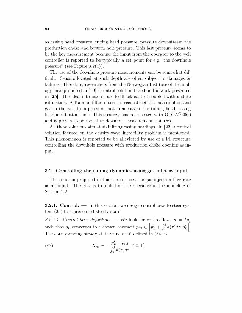
84 CHAPTER 3. CONTROL SOLUTIONS
as casing head pressure, tubing head pressure, pressure downstream theproduction choke and bottom hole pressure. This last pressure seems tobe the key measurement because the input from the operator to the wellcontroller is reported to be“typically a set point for e.g. the downholepressure” (see Figure 3.2(b)).
The use of the downhole pressure measurements can be somewhat dif-ficult. Sensors located at such depth are often subject to damages orfailures. Therefore, researchers from the Norwegian Institute of Technol-ogy have proposed in [19] a control solution based on the work presentedin [25]. The idea is to use a state feedback control coupled with a stateestimation. A Kalman filter is used to reconstruct the masses of oil andgas in the well from pressure measurements at the tubing head, casinghead and bottom-hole. This strategy has been tested with OLGAr2000and is proven to be robust to downhole measurements failures.
All these solutions aim at stabilizing casing headings. In [23] a controlsolution focused on the density-wave instability problem is mentioned.This phenomenon is reported to be alleviated by use of a PI structurecontrolling the downhole pressure with production choke opening as in-put.
3.2. Controlling the tubing dynamics using gas inlet as input
The solution proposed in this section uses the gas injection flow rateas an input. The goal is to underline the relevance of the modeling ofSection 2.2.
3.2.1. Control. — In this section, we design control laws to steer sys-tem (35) to a predefined steady state.
3.2.1.1. Control laws definition. — We look for control laws u = λqg
such that pL converges to a chosen constant pref ∈]
p?L +
∫ δ
0k(τ)dτ, p?
L
[
.
The corresponding steady state value of X defined in (34) is
Xref = − p?L − pref∫ δ
0k(τ)dτ
∈]0, 1[(87)

3.2. CONTR. TUBING DYN. USING GAS INLET AS INPUT 85
X
pt(L)qg
pr
f(pt(L), pr, Xref)
Figure 3.3. Control strategy using gas inlet as input. We
feed the tubing with a computed gas flow rate qg such that the
gas mass fraction at the bottom of the tubing is equal to Xref .
This computation takes the bottom-hole pressure pt(L) and the
reservoir pressure pr into account.
We note uref the value of u at steady state. It satisfies
Xref(uref) =p?
L − pr + uref
uref −∫ δ
0k(τ)dτ
(88)
Our (closed-loop) control law is, simply,
u(t) =pr − pL(t)
1−Xref
(89)
Figure 3.3 illustrates this strategy.This control strategy feeds system (35), which has finite memory δ,
with a constant term. By direct computation, this straightforward ap-proach provides convergence. We can state the following proposition.
Proposition 9. — With control law (89), pL which dynamics is defined
by system (35) converges to pref in finite time δ for any initial condition
[−δ, 0] 3 t 7→ φ(t) ∈ R.

86 CHAPTER 3. CONTROL SOLUTIONS
Yet, the expression u defined in (89) does not take into account actu-ation saturations. Here, the most limiting factor in practice is a lowerbound umin > 0 on the control. In facts, some simulations show that thisconstraint is often reached with this naive approach. We now proposethe saturated control law
(90)
u =pr − pL(t)
1−Xref
, for pL < pr − umin(1−Xref)
u = umin, for pL ≥ pr − umin(1−Xref)
Proposition 10. — Assume that
Xref ≥p?
L − pr + umin
umin −∫ δ
0k(τ)dτ
(91)
With the (saturated) control law (90), pL which dynamics is defined by
system (35), converges to pref in finite time 2δ for any initial condition
[−δ, 0] 3 t 7→ φ(t) ∈ R.
Proof. — We now show that, for t ≥ δ, the control law is unsaturated.Indeed, for t > 0
h
(
1− pr − pL(t)
u(t)
)
≥ Xref
Therefore, for all t ∈ [δ,+∞[,
pL(t) ≤ p?L +Xref
∫ δ
0
k(τ)dτ
Assuming (91), a simple computation yields
∀t ≥ δ, pL(t) ≤ pr − umin(1−Xref)
By equation (90), we get that, for all t ≥ δ, u is simply defined by
u =pr − pL(t)
1−Xref
The control is thus unsaturated and, by Proposition 9, we conclude thatsystem (35) converges towards pref in 2δ.
In practice, one must choose pref in accordance to the minimumvalue umin such that equation (88) holds. This choice implies that as-sumption (91) holds.
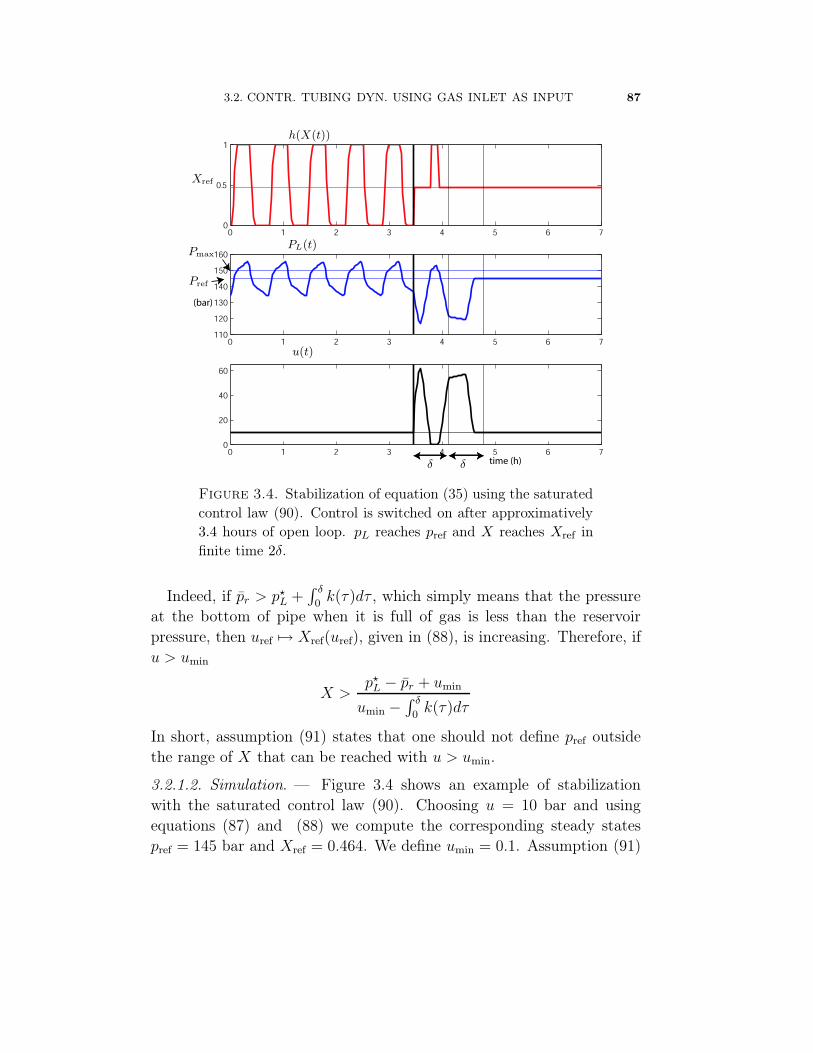
3.2. CONTR. TUBING DYN. USING GAS INLET AS INPUT 87
0 1 2 3 4 5 6 70
0.5
1
0 1 2 3 4 5 6 7110
120
130
140
150
160
0 1 2 3 4 5 6 70
20
40
60
(bar)
time (h)
Xref
h(X(t))
Pmax
Pref
PL(t)
u(t)
δδ
Figure 3.4. Stabilization of equation (35) using the saturated
control law (90). Control is switched on after approximatively
3.4 hours of open loop. pL reaches pref and X reaches Xref in
finite time 2δ.
Indeed, if pr > p?L +
∫ δ
0k(τ)dτ , which simply means that the pressure
at the bottom of pipe when it is full of gas is less than the reservoirpressure, then uref 7→ Xref(uref), given in (88), is increasing. Therefore, ifu > umin
X >p?
L − pr + umin
umin −∫ δ
0k(τ)dτ
In short, assumption (91) states that one should not define pref outsidethe range of X that can be reached with u > umin.
3.2.1.2. Simulation. — Figure 3.4 shows an example of stabilizationwith the saturated control law (90). Choosing u = 10 bar and usingequations (87) and (88) we compute the corresponding steady statespref = 145 bar and Xref = 0.464. We define umin = 0.1. Assumption (91)

88 CHAPTER 3. CONTROL SOLUTIONS
P0
qgqgqgqgXref
x(t, z)
xL(t)
qlqlqlql
Pr
Figure 3.5. Comparison of open loop (3 schemes on the left)
and closed loop behavior.
holds. Until tc the system is left open loop. At t = tc, the controller isturned on. From tc to tc + δ, the gas mass fraction h(X(t)) remainsbetween Xref and 1. Therefore, for t > tc + δ, Pl(t) remains belowPmax = pr − umin(1 − Xref) = 150 bar and h(X(t)) = Xref. PressurepL converges to pref in finite time.
An alternative view is given in Figure 3.5. Left three snapshots de-scribe the open-loop behavior. Gas mass fraction profile (x(t, z)) is repre-sented in white (complementary black part stands for oil mass fraction).Boundary condition qg is constant and ql is defined by equation (31).Finally, the right scheme represents the transient obtained with closedloop control. The feeds keep the gas mass ratio constant at Xref. Duringthe transient, qg is permanently adapted to counteract the effect of thestate x(t, z), z ∈ [0, L], onto ql. This yields a constant X(t, L) whichprogressively steers the system to steady state through the transportequation.

3.2. CONTR. TUBING DYN. USING GAS INLET AS INPUT 89
3.2.1.3. Stabilization of the well simulated in OLGAr2000. — Theclosed loop control law can be tested in OLGAr2000. In Section 2.2.2.1,we assume the gas velocity to be constant, i.e. we neglect the impact ofthe gas mass fraction on the gas velocity. Therefore, when the gas massflow rate is high enough, this assumption only results in a time scaling.But, when the gas inlet is too low, the well production eventually stops,which is not represented by the simple model. Therefore, we want thegas injection rate to remain above a minimum, qmin
g , guaranteeing thatan actual flow takes place in the pipe. This defines a lower bound for ourcontrol law. Following the same lines as in the section 3.2.1.1, we definethe control qg, corresponding to u (see equation (33)), to keep xL at a
0 1 2 3 4 5 6 70
0.5
1
0 1 2 3 4 5 6 780
100
120
140
160
0 1 2 3 4 5 6 70
0.5
1
1.5
0 1 2 3 4 5 6 70
20
40
60
(bar)
(kg/s)
(kg/s)
time (h)
Reservoir pressure Pr
Gas mass fraction at the bottom
Oil flow rate at well head
Gas injection rate
Xref
qmin
g
Figure 3.6. Stabilization of density wave instability simulated
in OLGAr2000 (numerical set up given in Appendix A, Ta-
ble 3). Xref = 0.0568 and qming = 0.3.

90 CHAPTER 3. CONTROL SOLUTIONS
predefined constant, Xref . Using xL given in equation (32), our controllaw writes
qg(t) = max
(
Xref
1−Xref
IP (pr − pL(t)), qming
)
Figure 3.6 represents an example of stabilization of the density waveinstability. We define qmin
g = 0.3 kg/s and Xref = 0.0568. The controlleris switched on at approximatively tc = 3.4 hour and steers the well to thesteady state corresponding to the initial gas injection rate. The period ofthe oscillations approximatively equals the travel time δ. One can see inFigure 3.6 that the well is stabilized in 2δ. As stated in Proposition 10, 2δ
corresponds to the time needed by the well to forget its initial condition.
3.3. Controlling the tubing dynamics using the productionchoke as input
production valve
gas inlet
u
pt(H)
Figure 3.7. Control of the
bottom hole flowing pressure
(pt(H)) with a PID controller
on the production choke (u).
There exists a strong obstacleto the previously presented con-trol technique. As discussed inSection 1.2.1.2, gas is allocatedscarcely between the wells. Be-cause the casing acts as a largebuffer tank located at the input ofthe tubing subsystem, any controllaw using the gas inlet as inputpotentially demands large peaksduring transients. To compen-sate the very slow casing dynam-ics, high gas flow rate variationsmust be considered. The inducedvariations need high gas availabil-ity. These requirements are incom-patible with the above mentionedconstraints. In practice, even forreasonably scaled transients, it isnot uncommon to punctually need

3.3. CONTR. TUBING DYN. WITH THE PRODUCTION CHOKE 91
OIL-INLET
RES SOURCE-GAS RCV
WELL-HEADTUBING
OIL-INLET
RES SOURCE-GAS
TUBINGWELL-HEAD
Figure 3.8. Block scheme of the OLGAr2000 simulation
setup. First case (top) with a production choke, second case
(bottom).
more than twice the nominal amount of gas. This issue prevents the gasinlet from being considered as an manipulated input (except for very lowfrequency signals).
Therefore, in this section, we propose a control strategy using theproduction choke as input (see Figure 3.7). The main advantage of thischoice is that it has a direct impact on the dynamics, unfortunately italso has a counter part: the choke has a very small active range.
3.3.1. Manipulated variable definition. — In a first approxima-tion, we model the production choke opening variations as tubing headpressure variations. Therefore, we investigate the role of the tubing wellhead pressure as input variable. With OLGAr2000 we consider two se-tups to simulate the flow in a single vertical pipe (see Figure 3.8). Oilis supplied by a reservoir and gas is injected at the bottom of the pipe.In the first setup, the pipe is equipped with a production choke that weprogressively open. In the second setup, there is no production choke.Instead, the tubing is modeled as a pipe with a downstream pressureboundary condition. Gradually, we decrease this boundary pressure,simulating a reduction of the well head pressure. This section is partof a work that appeared in the International Symposium on AdvancedControl of Chemical Processes, 2006 (see [35]).
Figure 3.10(a) shows the steady state well head pressure values asa function of the production choke opening. Classically, our focus is

92 CHAPTER 3. CONTROL SOLUTIONS
0 50 100 150 200 250 300 350 4004.84
4.85
4.86
4.87
0 50 100 150 200 250 300 350 4004.71
4.72
4.73
4.74
4.75
Time [min]
Step response to an increase of the well head pressure
Oil
vel
oci
ty[m
/s]
Oil
vel
oci
ty[m
/s]
Step response to a decrease of the choke opening
Figure 3.9. Comparison of the step responses to an increase
of the well head pressure and to a decrease of the production
choke opening.
on comparing the oil and gas velocities histories obtained from the twosimulation setups. Figure 3.10(b) reports the static values of the oil andgas velocities as a function of the well head pressure. Over almost thewhole well head pressure operating range (from 23 to 29 bar, i.e. from0.2 to 1 choke opening), the curves coincide. It is only when the choke isalmost closed that differences appear. Figure 3.9 shows the comparisonof the step responses to an increase of the well head pressure and to aconsistent decrease of the production choke opening, respectively. Wenotice similar undershoots of approximately 0.02 m/s. It takes betweenfour and five noticeable oscillations for both systems to settle. Thisexperiment suggests it is valid to consider pt(0) as our input variable.From now on, we denote u , pt(0).
3.3.2. Open loop stability analysis. — Recall equation (35)
pt(t, L) = pt(0) + cst+
∫ t
t−δ
k(t− ζ)h(
1− pr − pt(ζ, L)
λqg(ζ)
)
dζ(92)
We assume that the gas injection in the tubing is constant. Linearizationyields

3.3. CONTR. TUBING DYN. WITH THE PRODUCTION CHOKE 93
0.1 0.2 0.3 0.4 0.5 0.6 0.7 0.8 0.9 122
23
24
25
26
27
28
29
30
Production choke opening [-]
Wel
lhea
dpre
ssure
[bar]
(a) Well head pressure as a function of the production
choke opening.
22 23 24 25 26 27 28 29 30 313.5
4
4.5
5
5.5
6
6.5
[m/s]
Well head pressure [bar]
Oil velocity
Gas velocity
(b) Comparison of the oil and gas velocities between
the fist and second cases (continuous and dashed line
respectively).
Figure 3.10. Steady state comparison of the impact of varia-
tions of tubing head pressure and production choke opening.

94 CHAPTER 3. CONTROL SOLUTIONS
δpt(t, L) = δu+
∫ δ
0
k(ζ)δpt(ζ − δ, L)
λqgdζ(93)
In Laplace coordinates,
δpt(s, L) =1
1− k(s)λqg
δu(s)(94)
Where k,the Laplace transform of k, writes
k(s) = k21− e−δs
s+k1
δ
1− e−δs − δse−δs
s2(95)
Using Nyquist criterion we know that the stability of the system whichtransfert writes as equation (95) is determined by the shape of the curvedefined by −k(jω)/(λqg) for ω ∈ [0,+∞). Since k(s) has no zero, if theNyquist plot does not encircle −1 the tubing dynamics is stable. Wewill not go through the complete stability analysis as it has already beenperformed in Section (2.2.3). We simply notice that the role of the gasinjection qg is played by as an homothety of the Nyquist plot. Besides,oneshould also notice notice that k(s, αδ) = αk(αs, δ), which means that an
-4 -2 0 2 4 6 8 10 12-10
-8
-6
-4
-2
0
2
4
6
8
10
Figure 3.11. Nyquist plot corresponding to the linearization
equation (35) for qg=0.2kg/s. The tubing dynamics is unstable.

3.3. CONTR. TUBING DYN. WITH THE PRODUCTION CHOKE 95
pt(L)
pr
pt(0)
IP
Figure 3.12. Control of the bottom hole pressure pt(L) with
the well head pressure pt(0).
increase of the delay also plays the role of an homothety. Figure 3.11represents the Nyquist plot corresponding to the transfer function (95)for qg = 0.2 kg/s. One notice that the tubing dynamics is unstable butclose to be stable, for qg = 0.3 kg/s it would be stable.
3.3.3. Closed loop stability analysis. — We will now show that,for all gas injection rate, the tubing dynamics can be stabilized eitherwith a P controller or with an IP controller (see Figure 3.12). In the IPcontroller case, the reference is only taken into account in the integralterm. It allows smooth responses when the reference is updated.
3.3.3.1. P controller. — Let us define the input u = pt(0) as follows
u = u0 − kp(pt(L)− preft (L))
The closed loop transfer writes
δpt(s, L) =kp/(1 + kp)
1− k(s)(1+kp)λqg
δpreft (s)(96)

96 CHAPTER 3. CONTROL SOLUTIONS
Proposition 11. — For all qg > 0 there exists kp > 0 such that the
closed loop system defined by equation (96) is stable.
Proof. — Recalling computations done in Section 2.2.3, we know thatthere exist a minimum gas injection qmin
g such that for all qg > qming , the
corresponding Nyquist plot does encircle -1. If qg < qming we just have to
define kp >qming
qg− 1.
3.3.3.2. Use of an IP controller. — Let us define the input u = pt(0) asfollows
u = u0 − kppt(L)− kp
Ti
∫ t
0
pt(L)− preft (L)(97)
with u0 defined such that pt(0+, 0) = pt(0
−, 0). It follows
u0 = pt(0, 0) + kppt(0, L)
In Laplace coordinates,
δu = −kp
(
1 +1
sTi
)
δpt(L) +1
sTiδpref
t (L)
The closed loop transfert writes
δpt(L) =kp/Ti/s
1− k(s)/(λqg) + kp
(
1 + 1sTi
)δpreft (L)(98)
=1
1 + Tis(
1 + 1kp
(
1− k(s)λqg
))δpreft (L)
Proposition 12. — For each qg one can find kp > 0 and Ti > 0 such
that the system which transfer writes as equation (98) is stable.
Proof. — Let G be defined by
G(s) = Tis
(
1 +1
kp
(
1− k(s)
λqg
))
Stability of the transfer (98) can be analyzed through the Nyquist plotof G(jω). Its real and imaginary parts are
Re(G(jω)) =Ti
kpλqgIm(ωk(jω))

3.3. CONTR. TUBING DYN. WITH THE PRODUCTION CHOKE 97
-1 -0.8 -0.6 -0.4 -0.2 0 0.2 0.4 0.6 0.8 1-8
-6
-4
-2
0
2
4
6
8
Figure 3.13. Nyquist plot of the closed loop tubing dynamics.The black line represents the lower boundary defined in
equation (99).
and
Im(ωk(jω)) = (k1 + k2) cos(ωδ)− k2 − k1sin(ωδ)
ωδ
Remembering that k1 and k2 are both strictly negative, we get the fol-lowing lower bound
Re(G(jω)) > 2k1Ti
kpλqg(99)
Therefore, choosing Ti > 0 and kp > 0 such that the following inequalityis verified guarantees the stability
Ti
kp< −λqg
2k1

98 CHAPTER 3. CONTROL SOLUTIONS
3.4. Controlling the well dynamics using production choke asinput
Up to this point we have shown that it is possible to control the tubingdynamics using the tubing head pressure as input and the bottom holepressure as output (as summarized in Figure 3.7). Unfortunately there isoften no sensor at the bottom of the well, and, when there are some, theyare usually subject to recurrent failures. It is a common thought that wecannot rely on such measurements. Therefore we have to complement theanalysis of the previous section with solutions to implementation issues.As shown in Figure 3.14 we propose to use the casing head pressure toestimate the bottom hole pressure.
CasingTubingpt(L) pc(0)
pt(L)
pt(0)
IPpt(L)ref
Estimator
Figure 3.14. Scheme of the proposed control and estimation architecture.
3.4.1. Bottom hole pressure estimation. — The casing head pres-sure is related to the bottom hole pressure through the gas volume con-tained in the annular part. Given the input gas flow rate and the massvariation (given by the pressure variations), one can easily derive theoutput gas flow. The last step consists in computing the pressure down-stream the gas injection valve, knowing the upstream pressure and theflow rate. This part presents the principles of an estimator software thathas been deposited on the “Agence pour la Protection des Programmes”under the Inter Deposit Number
IDDN.FR.001.340008.000.R.P.2006.000.30400

3.4. CONTR. WELL DYNAMICS WITH PRODUCTION CHOKE 99
3.4.1.1. Estimator definition. — We recall equation (69)
m1 = qgi − qg(m1, pt(L))
qg(m1, pt(L)) = Cg
√
µm1 max(νm1 − pt(L), 0)
We just have to express m1 in term of pc(0) through the ideal gas law
pc(0) =RTc
VcMm1 = ξ′m1
Assuming that the bottom hole pressure is slowly varying comparedto the casing dynamics, we estimate pt(L) thanks to the following model
pc(0) = ξ′(
qgi − Cg
√
µ′pc(0) max(ν ′pc(0)− pt(L), 0))
pt(L) = 0
with µ′ = µξ′
and ν ′ = νξ′
.We define the following estimator
(100)
˙pc(0) = ξ′(
qgi − Cg
√
µ′pc(0) max(ν ′pc(0)− pt(L), 0))
− l1(pc(0)− pc(0))
˙pt(L) = −l2(pc(0)− pc(0))
3.4.1.2. Estimator physical interpretation. — Linearization of equa-tion (100) yield
(
δ ˙pc(0)
δ ˙pt(L)
)
=
(
−r t
0 0
)(
δpc(0)
δpt(L)
)
−(
l1l2
)
(δpc(0)− δpc(0))
where r and t are two positive constants. Therefore, considering that thisestimator is a filter which input is δpc(0) and which output is δpt(L), itstransfer writes
δpt(s, L) =s+ r
s2
l2+ l1s
l2+ t
δpc(s, 0)(101)
Using a high gain l2, this transfer reduces to
s+ r
t

100 CHAPTER 3. CONTROL SOLUTIONS
which means that this filter locally inverts the casing dynamics. Noticethat this transfer is not causal (while transfert (101) is), which will leadto some implementation issues.
3.4.1.3. Impact of modeling errors. — Denote ec = pc(0) − pc(0) andet = pt(L) − pt(L) the coordinates of the error vector between the realtrajectory and the estimated one. The dynamics of the error writes
(
ec
et
)
=
(
−ξ′(qg(pc(0), pt(L))− qg(pc(0), pt(L)))− l1ec
−l2ec
)
This means that the estimator dynamics converges towards a trajectory(pc(0), pt(L)) which verifies
qg(pc(0), ˆpt(L)) = qg(pc(0), pt(L))
As qg is a bijective function with respect to its second variable for pt(L) <
ν ′pc(0) this defines, in this region, pt(L) as
pt(L) = pt(L)
Now assume that the qg function is not perfectly known and that theconstant ν ′ and µ′ are linear biased. We define
qg = Cg
√
µ′pc(0) max(ν ′pc(0)− pt(0))
with ν ′ = (1 + ε)ν, µ′ = (1 + ε)µ and ε a small constant error. Thetrajectory (pc(0), pt(L)) is now defined by
qg(pc(0), ˆpt(L)) = qg(pc(0), pt(L))
Assuming that qg and qg are not equal to zero, we get that
pt(L) =1
1 + εpt(L)− ε(2 + ε)
1 + εpc(0)
This means that the estimator probably reconstructs an affine biasedvalue of pt(L). This is not an issue. We do not need a precise value forpt(L), we just need to get enough information of the system behavior tobe able to stabilize it. An affine biased reconstruction is enough.
We can easily get rid of the constants. As we define the reference forpt(L) based on its estimation we do as if we knew the value of the biases.

3.4. CONTR. WELL DYNAMICS WITH PRODUCTION CHOKE 101
Therefore in the definition of the IP controller (97) becomes
u = u0 − kp1
1 + εpt(L) + kp
ε(2 + ε)
1 + εpc(0)− kp
Ti
1
1 + ε
∫ t
0
pt(L)− preft (L)
with
u0 = pt(0, 0) + kp1
1 + εpt(0, L)− kp
ε(2 + ε)
1 + εpc(0, 0)(102)
In practice the term ε(2+ε)1+ε
(pc(0, t)− pc(0, 0)) is very close to 0 and doesnot perturb the convergence of the controller.
3.4.1.4. Simulations results. — Figure 3.15 shows simulations exampleof bottom hole estimation. The scenario is the following: at first thechoke opening is set to 0.2, which correspond to a stable set point. Thewell tends to stabilize. Then, at time t=300 min, the choke is openedup to 0.34. This corresponds to an unstable set point. In both cases theestimator correctly reconstructs the bottom hole pressure. Notice that,while convergence is almost instantaneous for pc(0), it takes a bit moretime for pt(L) to settle. Moreover the behavior of pt(L) is not as smoothas the one of the reconstructed casing head pressure. In this case, theconvergence is perfect because we perfectly know the function qg.
3.4.2. Experimental results. — Figure 3.16 shows experimental re-sults obtained on a TOTAL operated well. The bottom hole pressurePt(L) is derived, thanks to the observer, from the casing head pressuremeasurements, Pc(0) and from the gas injection flow rate measurements,Qg. The estimated pressure is compared with the tubing head pressure,Pt(0), to validate the relevance of the approach. In Figure 3.16 the wellis unstable. The oscillations are very regular and their period is close tothe propagation time. The tubing head pressure is used to monitor theexpulsions of the liquid slugs, which correspond to the pressure peaks.Each of these peak is followed by a drop of the estimated bottom holepressure, this is relevant with the description of the density-wave phe-nomenon. The bottom hole pressure estimation behaves as predicted:it decreases when the tubing head pressure increases which correspondsto the arrival of the liquid-rich slug and then it increases as the tubing

102 CHAPTER 3. CONTROL SOLUTIONS
0 100 200 300 400 500 600120.2
120.4
120.6
0 100 200 300 400 500 600130
131
132
133
0 100 200 300 400 500 60024
25
26
27
0 100 200 300 400 500 6000.2
0.3
0.4
Pt(0
)[b
ar]
Pc(0
)[b
ar]
Qg
[kSm
3/j]
Time [min]
Ψ[−
]
estimatedreal
Figure 3.15. Estimation of the bottom hole pressure using
the casing head pressure in OLGAr2000 simulation (numerical
set up is given in Appendix A, Table 4). Solid blue (reference
from OLGAr2000), dotted red estimation.
head pressure drops, at the end of the liquid-rich slug. Moreover thereconstructed values of Pt are coherent with steady state computations.
3.4.3. Controller results. — Figure 3.17 shows simulations exampleof a closed loop stabilization. The scenario is the following: at firstthe choke opening is set to 0.2, which corresponds to a stable set point.The well tends to stabilize. Then, at a time less than t=100 min, thecontroller is switched on. The reference for the pressure pt(L) is set to131.7 bar which corresponds to an unstable point. In both cases theestimator correctly reconstructs the bottom hole pressure. The well isstabilized.

3.4. CONTR. WELL DYNAMICS WITH PRODUCTION CHOKE 103
0 1000 2000 3000 4000 5000 60000
0.2
0.4
0.6
0.8
1
0 1000 2000 3000 4000 5000 60000
0.2
0.4
0.6
0.8
1Pt(0)
Pc(0)
Pt(L)
Figure 3.16. Experimental results on a TOTAL operated well
over more than half a day. The bottom hole pressure, Pt(L),
is reconstructed from the casing head pressure and from the
gas injection flow rate measurements, respectively, Pc(0) and
Qg. The estimated pressure is compared with the tubing head
pressure, Pt(0), to highlight the relevance of the results (for
confidentiality reasons, scales have been omitted).

104 CHAPTER 3. CONTROL SOLUTIONS
0 100 200 300 400 500 600 700 800 900
0.2
0.25
0.3
0 100 200 300 400 500 600 700 800 900120.4
120.5
120.6
0 100 200 300 400 500 600 700 800 900131.4
131.6
131.8
0 100 200 300 400 500 600 700 800 900
25
26
real
real
real
Time [min]closed lo
open
loop
estimated
estimated
reference
open loop
Figure 3.17. Closed loop stabilization example in
OLGAr2000 simulation (numerical set up is given in
Appendix A, Table 4). The choke opening Ψ is first set to
0.2 which corresponds to a stable equilibrium. The tubing
pressure downstream the injection valve (Pt(L)) is equal to
131.7 bar. The reference for Pt(L) is set to 131.5 bar. After
approximately 100 min the controller is switched on. All
pressures converge towards constant values. Notice that the
estimator is well behaving: the estimation of Pt(0) and of the
casing head pressure, Pc(0), are relevant.

CONCLUSION
Dans ce mémoire consacré à l’étude des puits pétroliers activés engas-lift nous avons cherché à apporter des solutions au problème pra-tique des instabilités d’écoulement fréquemment constaté sur les instal-lations. Principalement, il a été constaté qu’en vieillissant les puits onttendance à produire moins et moins bien. Leur production, constituéed’une succession de bouchons dont la répartition gaz/liquide est haute-ment fluctuante, est alors qualifiée d’instable. Ce type de comportementsest préjudiciable. Il diminue la production moyenne du puits concerné,risque de se propager aux puits connectés sur les mêmes réseaux et égale-ment de créer des arrêts de production. Ces instabilités étant à la sourcede nombreux manques à produire, il est crucial de savoir les éviter, lessupprimer ou du moins les gérer. C’est le thème principal de notre étude.
Dans une première approche nous ne nous autorisons pas d’autres ac-tions sur le puits que le choix des conditions opératoires. Il s’agit dedéfinir un critère garantissant la stabilité du système en boucle ouverte.Nous acceptons de sacrifier l’accès à certaines zones à fort rendement.Dans une seconde approche nous choisissons de nous placer délibérémentdans ces zones en recourant à des contrôleurs en boucle fermée.
Dans l’étude en boucle ouverte nous proposons des modèles dontl’analyse nous permet de définir des critères de stabilité. Dans la littéra-ture, la dynamique de l’écoulement est généralement négligée ce qui per-met de réduire le système à un modèle à trois dimensions. Dans la thèsenous avons commencé par montrer que l’un des mécanismes d’instabilité,

106 CONCLUSION
le casing-heading, pouvait effectivement être analysé de cette façon. Ladynamique peut en fait se restreindre à deux dimensions et le phénomènes’interpréter comme un cycle limite dans un plan. Malheureusement cetteapproche ne couvre pas tous les cas pratiques. En effet un deuxième mé-canisme, la density-wave, provient justement (comme nous l’avons dé-montré) de l’écoulement dans le puits et du retard lié à la propagationdes effluents du réservoir à la surface. Une des contributions principalesde cette thèse est de proposer un modèle à paramètres distribués quipermet de modéliser le puits et d’analyser le phénomène d’instabilité parl’étude des racines d’une équation du type
s = a+ be−sτ +c
sτ(1− e−sτ )
où τ est le temps de propagation dans le puits. Il est possible d’unifierles deux approches. Nous proposons un modèle global, constitué du cou-plage de l’équation à paramètres distribués et d’un système dynamiquedu premier ordre. Nous faisons apparaître, dans le système physique,deux boucles de rétroaction (représentées sur la Figure 3.18) qui peu-vent être positives . L’impact des principaux paramètres physiques surla stabilité a été étudié et ainsi un certain nombre de règles opératoiresempiriques ont pu être théoriquement validées. Les critères que nousproposons sont qualitatifs et non quantitatifs. En effet, les paramètresphysiques du puits sont connus avec trop d’imprécision et varient telle-ment que ce critère n’aurait pas de sens.
Ce modèle nous sert de référence pour la conception de stratégies decontrôle en boucle fermée. Nous proposons une loi de commande. Les ré-sultats obtenus en simulation sont probants. Les puits simulés en bouclefermée sont capables de produire de façon stable lorsque la vanne de pro-duction est très ouverte, ce qui est impossible en boucle ouverte. Leszones à haut rendement sont donc accessibles.
La pertinence de l’approche et des modèles proposés a été validée grâceaux résultats obtenus en simulation et surtout grâce aux résultats partielsobtenus sur site de production (présentés dans ce document). De nom-breux problèmes d’implémentation doivent être résolus. En particulier,nous avons montré sur site qu’il était possible d’estimer la pression defond en n’utilisant que des mesures obtenues à la surface.

CONCLUSION 107
Pression de fond
Gaz
Gaz injecté
tubing
casing
Figure 3.18. Représentation du puits sous forme d’un schéma
bloc. Les instabilités correspondent aux boucles de rétroaction
potentiellement positives représentées par les flèches rouges.
Aujourd’hui, ces résultats nous ouvrent l’accès à des essais sur site dela loi de commande. Les résultats préliminaires sont très satisfaisants.Dans ce cadre d’industrialisation, un travail complémentaire d’analysede robustesse est nécessaire, de façon à garantir l’efficacité dans le plusgrand nombre de configurations possibles.
This report is dedicated to the study of gas lift activated oil wells. Weaimed at bringing solutions to the recurrent problem of flow instabili-ties. It has been noticed, in the literature, that, over time, wells tendto produce less in quantity and quality. Eventually, their productionflow consists of a succession of slugs, whose gas/liquid ratio is highlyfluctuating. This behavior should be avoided: it decreases the averageproduction rate of the well, it might propagate to other connected wellsand possibly cause production stops. These instabilities yield importantproduction losses and it is interesting to know how to avoid them, getrid of them or at least how to handle them. This is the goal of our study.

108 CONCLUSION
In a first approach we decided not to consider any other actions besideschoosing operating conditions. We defined a criterion which guaranteesthe open-loop system stability. This approach has a cost, because highreturn zone are most likely unreachable. In a second approach we choseto precisely pick operating conditions in the high return zone. The sta-bilization is achieved thanks to closed loop controller.
In the open-loop setup, we propose models from which stability criteriawere derived. In the literature, the flow dynamics is often neglected. Thisallows to reduce the system dynamics to a three-dimensional model. Inthis report we first showed that one of the unstable mechanisms, thecasing-heading, could be analyzed using this reduction. The phenomenonwas interpreted as a limit cycle in the plane. Unfortunately, this approachdoes not address all issues. In the case of the second mechanism, thedensity-wave, the instability arises (as we have explained it) from theflow regime and from the propagation delay between the bottom of thewell and the surface. Our main contribution is to interpret the system asa distributed parameters model and to analyse the density-wave thanksto the study of the roots of the equation
s = a+ be−sτ +c
sτ(1− e−sτ )
where τ is the propagation time in the well. Finally, these two approachescan be combined. We proposed a global model, which consists in thecoupling of the distributed parameters equation and a first order dy-namical system. We highlighted the existence of two possibly positivefeed-forward loops (represented on Figure 3.19). We studied the impacton the stability of the main physical parameters. Our results are in accor-dance with operating rules-of-the-thumb. We propose qualitative (andnon quantitative) criteria. Deriving quantitative criteria from impreciseand possibly not up-to-date data records did not appear to us as a robustsolution.
Rather, this model suggested a closed loop control strategy design.We proposed a control law. The results obtained in simulations stressthe relevance of this approach. The closed loop simulated wells are ableto produce steadily, even of large production choke openings. This is

CONCLUSION 109
Bottom hole pressure
Gas
Injected gas
tubing
casing
Figure 3.19. Block scheme the well as an interconnected sys-
tem. The possibly positive feedback loops are in red.
not doable in open-loop. With feedback control, high return zones arereachable.
The relevance of the approach and of the proposed models has beenvalidated thanks to simulations results and also mainly thanks to on-siteresults (presented in this document). Several implementations issues hadto be solved. In particular, we showed, on site and in real time, how toreconstruct the bottom hole pressure measurements, using only surfacemeasurements.
Now, this results give us access to broad field tests. Preliminary resultsare very promising. In the context of industrial use, a complementarystudy on the robustness of the solution is needed to guarantee the effi-ciency in the widest range of possible configurations.


APPENDIX A
OLGAr2000 SIMULATIONS SETTINGS
Table 1. Numerical set-up for Figure 1.3
Symb. Description Values Unitsφ injection valve orifice diameter 15.5/64 inchQgi gas injection flow rate 28-220 kSm3/jqgi gas injection flow rate 0.01-7 kg/sPI Productivity Index 10−5
pr Reservoir pressure 150 bar
Table 2. Numerical set-up for Figure 2.2
Symb. Description Values Unitsφ injection valve orifice diameter 17.2/64 inchQgi gas injection flow rate 25 kSm3/jqgi gas injection flow rate 0.2 kg/sPI Productivity Index 10−6
pr Reservoir pressure 180 bar

112 APPENDIX A. OLGAr2000 SIMULATIONS SETTINGS
Table 3. Numerical set-up for Figure 2.9 and Figure 3.6
Symb. Description Values Unitsφ injection valve orifice diameter 12.8/64 inchQgi gas injection flow rate 62.5 kSm3/jqgi gas injection flow rate 0.6 kg/sPI Productivity Index 4−6
pr Reservoir pressure 150 bar
Table 4. Numerical set-up for Figure 3.15 and Figure 3.17
Symb. Description Values Unitsφ injection valve orifice diameter 12.8/64 inchQgi gas injection flow rate 25 kSm3/jqgi gas injection flow rate 0.2 kg/sPI Productivity Index 10−5
pr Reservoir pressure 150 barΨ Choke opening 0.2-0.317 -
Remark: The injection valve diameter is computed from OLGAr2000simulations to fit the following rule of the thumb, based on two assump-tions :
– if φ = 8/64 inch and if the flow is critical and if the upstreampressure is equal to 70 bar, then the flow rate will be 8 kSm3/j
– critical flow is obtained when the downstream pressure is less thanhalf the upstream pressure.
Qg = 2 ∗ 8/70
(
φ
8
)2√
Pt(L)(Pc(L)− Pt(L))(103)

APPENDIX B
NOMENCLATURE
Symb. Description Unitsa, b, c parameters of the distributed parame-
ters equation-
Cg constant of the gas valve S.ICpc constant of the production choke S.Ig gravity constant 9.81 m/s2
H reservoir depth mL injection depth mM molar mass of air 0.029 kg/molm1 mass of gas in the casing kgm2 mass of gas in the tubing kgm3 mass of liquid in the tubing kgpc(L) pressure in the casing at the injection
pointPa
pr reservoir pressure Papr appearing reservoir pressure Paps separator pressure Papt(0) pressure at the tubing wellhead Papt(H) pressure at the bottom-hole Papt(L) pressure in the tubing at the injection
pointPa
pt(L)ref reference set point for the pressure in thetubing at the injection point
Pa

114 APPENDIX B. NOMENCLATURE
Symb. Description Unitspt(0)con reference set point for the pressure in the
tubing at the wellheadPa
PI productivity index 4e− 6 kg/s/Paqg gas mass flow rate injected in the tubing kg/sqgi gas mass flow rate injected at the casing
wellheadkg/s
qming saturation value of qg 0.3 kg/sqlp liquid mass flow rate produced at the
wellheadkg/s
ql liquid mass flow rate produced from thereservoir
kg/s
qls liquid mass flow rate from the separator kg/sR ideal gas constant 287 S.I.rg(t, z) gas volume fraction -rl(t, z) oil volume fraction -Sc equivalent section of the casing m2
St tubing section m2
Tt temperature of the tubing 293 KTc temperature of the casing 293 Kx(t, z) gas mass fraction -xL(t) gas mass fraction at z = L
Vc casing volume m3
vl(t, z) oil velocity m/sv∞ slip velocity constant m/svg gas velocity 0.8 m/sβ threshold parameter 0.03δ tubing propagation time sΦl(t, z) oil mass flux kg/s/m2
Φg(t, z) gas mass flux kg/s/m2
Ψ production choke opening -ρc(H) gas density in the casing at the injection
pointkg/m3
ρg(t, z) gas density kg/m3
ρl density of oil 800 kg/m3

APPENDIX B. NOMENCLATURE 115
Symb. Description Unitsρm(t, z) mixture density kg/m3
Table 1: Nomenclature
All symbols in small letters have S.I. units. c indice denotes variablesrelating to the casing, t the tubing g the gas and l the oil, respectively.


LIST OF FIGURES
1.1 Typical oil production process system (schematic borrowedfrom [29]). . . . . . . . . . . . . . . . . . . . . . . . . . . . . . . . . . . . . . . . . . . . . . . . . 14
1.2 Scheme of a gas-lift activated well. . . . . . . . . . . . . . . . . . . . . . . . . 17
1.3 Performance curve (liquid production Qlp with respect to gasinjection flow rate Qgi) derived from OLGAr2000 simulations(numerical set up given in Appendix A, Table 1). Theblack star shows the optimum gas-lift injection Qopt
gi for giveneconomic conditions. . . . . . . . . . . . . . . . . . . . . . . . . . . . . . . . . . . . . . . 20
1.4 Schematic of an onshore installation. Wells are linked togetherthrough three networks: the gas network, the productionnetwork and the reservoir . . . . . . . . . . . . . . . . . . . . . . . . . . . . . . . . . . 22
1.5 Well instabilities example. Wellhead pressure, temperatureand oil flow from the separator are represented. An almostperiodic regime appears while oil production is intermittent.Scales are omitted for confidentiality reasons (courtesy ofTOTAL). . . . . . . . . . . . . . . . . . . . . . . . . . . . . . . . . . . . . . . . . . . . . . . . . . . 23
2.1 Schematic of the well. Zones of consideration (well head zone,bottom hole zone) appear in gray. . . . . . . . . . . . . . . . . . . . . . . . . . . 28
2.2 Unstable well behavior, casing heading, obtained with qgi =
0.2kg/s simulated with OLGAr2000 (numerical set up given

118 LIST OF FIGURES
in Appendix A, 2). The four main stages of the phenomenonare highlighted. . . . . . . . . . . . . . . . . . . . . . . . . . . . . . . . . . . . . . . . . . . . . 29
2.3 Scheme of the well and notations used in equation (2) (thecasing and the tubing part have been artificially separated toimprove readability). . . . . . . . . . . . . . . . . . . . . . . . . . . . . . . . . . . . . . . 31
2.4 Unstable well behavior, casing heading, obtained with qgi =
0.2kg/s simulated with equation (2) . . . . . . . . . . . . . . . . . . . . . . . . 32
2.5 Performance curve corresponding to the model (2) with gasinjection rate qg ranging from 0.01 to 7 kg/s and a liquidproduction from 3 to 17kg/s. Stable equilibrium points arerepresented in green and unstable in red. . . . . . . . . . . . . . . . . . . 34
2.6 Roots of model (2) are represented in the complex plane forgas injection ranging from 0.01 to 7 kg/s. Color axis goes from0 to 100% of the gas injection range. . . . . . . . . . . . . . . . . . . . . . . 35
2.7 Limit cycle (in blue) and positive invariant set (rectangleP1P2P3P4) for the sample problem. Switching curves ∂F o
g and∂F o
gp are represented. . . . . . . . . . . . . . . . . . . . . . . . . . . . . . . . . . . . . . . 44
2.8 Density wave occurring on a well. Casing-head and tubing-head pressures (respectively pc(0) and pt(0)) are representedas well as oil flow from the separator (Qls). Notice that thecasinghead pressure is almost constant, which demonstratesthat the gas injection is constant. Scales are omitted forconfidentiality reasons (courtesy of TOTAL). . . . . . . . . . . . . . . 47
2.9 Density wave simulated with OLGAr2000 (numerical set upis given in Appendix A, Table 3). . . . . . . . . . . . . . . . . . . . . . . . . . . 48
2.10 Scheme of the tubing. . . . . . . . . . . . . . . . . . . . . . . . . . . . . . . . . . . . . . . 49
2.11 Density wave simulated with equation (35). The reservoirpressure Pr is 150 bar and λqg is set at 10 bar. . . . . . . . . . . . . 54
2.12 Case (1) : φ(0) ∈ (0, 1). The trajectory converges towards aconstant also comprised between 0 and 1. . . . . . . . . . . . . . . . . . . 65
2.13 Cas 2. Depending on whether the Condition (55) is satisfiedthe trajectory converge betweens 0 and 1 or above 1. . . . . . . 66

LIST OF FIGURES 119
2.14 Block scheme of the tubing subsystem linearized aroundan equilibrium point. Gravitational effects of thenonhomogeneous fluid column take the form of an innerpositive feedback loop. . . . . . . . . . . . . . . . . . . . . . . . . . . . . . . . . . . . . 69
2.15 Simulation in OLGAr2000 of the impact of the pressurereservoir on the stability of the well. . . . . . . . . . . . . . . . . . . . . . . 72
2.16 (a) Outline of the casing. (b) The inputs of the system are thegas mass injection rate qgi and the boundary condition pt(L)
(the downhole pressure). The output is the gas rate enteringthe tubing: qg. . . . . . . . . . . . . . . . . . . . . . . . . . . . . . . . . . . . . . . . . . . . . 73
2.17 Block scheme of the interconnected systems linearized aroundan equilibrium point. . . . . . . . . . . . . . . . . . . . . . . . . . . . . . . . . . . . . . . 75
3.1 Some of the control solutions proposed in the literature. . . . . 81
3.2 More control solutions proposed in the literature. . . . . . . . . . . 82
3.3 Control strategy using gas inlet as input. We feed the tubingwith a computed gas flow rate qg such that the gas massfraction at the bottom of the tubing is equal to Xref . Thiscomputation takes the bottom-hole pressure pt(L) and thereservoir pressure pr into account. . . . . . . . . . . . . . . . . . . . . . . . . . . 85
3.4 Stabilization of equation (35) using the saturated controllaw (90). Control is switched on after approximatively 3.4
hours of open loop. pL reaches pref and X reaches Xref in finitetime 2δ. . . . . . . . . . . . . . . . . . . . . . . . . . . . . . . . . . . . . . . . . . . . . . . . . . . . . 87
3.5 Comparison of open loop (3 schemes on the left) and closedloop behavior. . . . . . . . . . . . . . . . . . . . . . . . . . . . . . . . . . . . . . . . . . . . . 88
3.6 Stabilization of density wave instability simulated inOLGAr2000 (numerical set up given in Appendix A, Table 3).Xref = 0.0568 and qmin
g = 0.3. . . . . . . . . . . . . . . . . . . . . . . . . . . . . . . 89
3.7 Control of the bottom hole flowing pressure (pt(H)) with aPID controller on the production choke (u). . . . . . . . . . . . . . . . . 90
3.8 Block scheme of the OLGAr2000 simulation setup. First case(top) with a production choke, second case (bottom). . . . . . . 91
120 LIST OF FIGURES
3.9 Comparison of the step responses to an increase of the wellhead pressure and to a decrease of the production chokeopening. . . . . . . . . . . . . . . . . . . . . . . . . . . . . . . . . . . . . . . . . . . . . . . . . . . 92
3.10 Steady state comparison of the impact of variations of tubinghead pressure and production choke opening. . . . . . . . . . . . . . . 93
3.11 Nyquist plot corresponding to the linearization equation (35)for qg=0.2kg/s. The tubing dynamics is unstable. . . . . . . . . . . 94
3.12 Control of the bottom hole pressure pt(L) with the well headpressure pt(0). . . . . . . . . . . . . . . . . . . . . . . . . . . . . . . . . . . . . . . . . . . . . 95
3.13 Nyquist plot of the closed loop tubing dynamics. The blackline represents the lower boundary defined in equation (99).. . . . . . . . . . . . . . . . . . . . . . . . . . . . . . . . . . . . . . . . . . . . . . . . . . . . . . . . . . . . 97
3.14 Scheme of the proposed control and estimation architecture.. . . . . . . . . . . . . . . . . . . . . . . . . . . . . . . . . . . . . . . . . . . . . . . . . . . . . . . . . . . . 98
3.15 Estimation of the bottom hole pressure using the casinghead pressure in OLGAr2000 simulation (numerical set upis given in Appendix A, Table 4). Solid blue (reference fromOLGAr2000), dotted red estimation. . . . . . . . . . . . . . . . . . . . . . . 102
3.16 Experimental results on a TOTAL operated well over morethan half a day. The bottom hole pressure, Pt(L), isreconstructed from the casing head pressure and from thegas injection flow rate measurements, respectively, Pc(0) andQg. The estimated pressure is compared with the tubing headpressure, Pt(0), to highlight the relevance of the results (forconfidentiality reasons, scales have been omitted). . . . . . . . . . . 103
3.17 Closed loop stabilization example in OLGAr2000 simulation(numerical set up is given in Appendix A, Table 4). The chokeopening Ψ is first set to 0.2 which corresponds to a stableequilibrium. The tubing pressure downstream the injectionvalve (Pt(L)) is equal to 131.7 bar. The reference for Pt(L) isset to 131.5 bar. After approximately 100 min the controller isswitched on. All pressures converge towards constant values.

LIST OF FIGURES 121
Notice that the estimator is well behaving: the estimation ofPt(0) and of the casing head pressure, Pc(0), are relevant. . . 104
3.18 Représentation du puits sous forme d’un schéma bloc.Les instabilités correspondent aux boucles de rétroactionpotentiellement positives représentées par les flèches rouges.. . . . . . . . . . . . . . . . . . . . . . . . . . . . . . . . . . . . . . . . . . . . . . . . . . . . . . . . . . . . 107
3.19 Block scheme the well as an interconnected system. Thepossibly positive feedback loops are in red. . . . . . . . . . . . . . . . . 109


BIBLIOGRAPHY
[1]
[2] “Standard handbook of petroleum and natural gas engineering,”W. C. Lyons, Ed. Gulf Professional Publishing, 1996.
[3] O. M. Aamo, G. O. Eikrem, H. Siahaan, and B. Foss, “Observerdesign for multiphase flow in vertical pipes with gas-lift - theoryand experiments,” Journal of Process Control, vol. 15, pp. 247–257,2005.
[4] F. J. S. Alhanati, Z. Schmidt, D. R. Doty, and D. D. Lageref, “Con-tinuous gas-lift instability: diagnosis, criteria, and solutions,” in 68th
Annual Technical Conference and Exhibition, no. SPE 26554, Hous-ton, TX, October 1993.
[5] H. Asheim, “Criteria for gas-lift stability,” Journal of Petroleum
Technology, pp. 1452–1456, November 1988.
[6] ——, “Criteria for gas-lift stability,” Journal of Petroleum Technol-
ogy, pp. 1452–1456, 1988.
[7] E. F. Blick and L. Boone, “Stabilization of naturally flowing oil wellsusing feedback control,” in Proc. of the 56th California Regional
meeting of the Society of Petroleum Engineers, no. SPE 15096, Oak-land,California, 1986.

124 BIBLIOGRAPHY
[8] E. F. Blick, P. N. Enga, and P. C. Lin, “Theoretical stability analysisof flowing oil wells and gas-lift wells,” SPE Production Engineering,pp. 508–514, 1988.
[9] E. F. Blick and A. B. Nelson, “Root locus stability analysis of aflowing oilwell feedback controller,” in Proc. of the SPE Production
Operations Symposium, no. SPE 18874, Oklahoma City, Oklahoma,1988.
[10] F. Brauer and J. A. Nohel, The qualitative theory of ordinary differ-
ential equations. An introduction. Dover Publications, INC. , NewYork, 1989.
[11] K. E. Brown, Gas lift theory and practice. Petroleum publishingCO., Tulsa, Oklahoma, 1973.
[12] H. Cholet, Well production. Practical handbook. Editions TECH-NIP, 2000.
[13] A. J. Chorin and J. E. Marsden, A mathematical introduction to
fluid mechanics. Springer-Verlag, 1990.
[14] R. F. Curtain and H. J. Zwart, An introduction to infinite-
dimensional linear systems theory, ser. Text in Applied Mathemat-ics, 21. Springer-Verlag, 1995.
[15] M. Dalsmo, E. Halvorsen, and O. Slupphaug, “Active feedback ofunstable wells at the Brage field,” in SPE Annual technical Confer-
erence and Exhibition, no. SPE 77650, 2002.
[16] W. J. G. J. der Kinderen, C. L. Dunham, and H. N. J. Poulisse,“Real-time artificial lift optimisation,” in Proc. of the 8th Abu Dhabi
International Petroleum Exhibition and Conference, 1998.
[17] E. Duret, “Dynamique et contrôle des écoulements polyphasiques,”Ph.D. dissertation, École des Mines de Paris, 2005.
[18] G. O. Eikrem, B. Foss, L. Imsland, B. Hu, and M. Golan, “Stabiliza-tion of gas-lifted wells,” in Proc. of the 15th IFAC World Congress,2002.

BIBLIOGRAPHY 125
[19] G. O. Eikrem, L. Imsland, and B. Foss, “Stabilization of gas-liftedwells based on state estimation,” in International Symposium on
Advanced Control of Chemical Processes, 2004.
[20] J. Faustinelli, G. Bermúdez, and A. Cuauro, “A solution to instabil-ity problems in continuous gas-lift wells offshore lake Maracaibo,”in Latin American and Caribbean petroleum engineering conference,
Caracas, Venezuela, no. SPE 53959, 1999.
[21] J. K. Hale and S. M. V. Lunel, Introduction to functional differential
equations. Springer-Verlag, 1993.
[22] I. A. Hiskens, “Stability of limit cycles in hybrid systems,” in Proc.
of the 34th Hawaii International Conf. on System Sciences, 2001.
[23] B. Hu and M. Golan, “Gas-lift instability resulted production lossand its remedy by feedback control: dynamical simulation results,”in SPE International Improved Oil Recovery Conference in Asia Pa-
cific, no. SPE 84917, Kuala Lumpur, Malaysia, 2003.
[24] L. S. Imsland, “Topics in nonlinear control - ouput feedback stabiliza-tion and control of positive systems,” Ph.D. dissertation, NorwegianUniversity of Science and Technology, Department of Engineeringand Cybernetics, 2002.
[25] L. S. Imsland, B. A. Foss, and G. O. Eikrem, “State feedback controlof a class of positive systems: application to gas lift stabilization,”in Proc. of the 7th European Control Conf., 2003.
[26] B. Jansen, M. Dalsmo, K. Havre, L. Nøkleberg, V. Kritiansen, andP. Lemétayer, “Automatic control of unstable gas-lifted wells,” inSPE Annual technical Confererence and Exhibition, no. SPE 56832,Houston,Texas, 1999.
[27] H. K. Khalil, Nonlinear Systems. MacMillan, 1992.
[28] P. Lemétayer and P. M. Miret, “Tool of the 90’s to optimize gas-lift efficiency in the Gonelle field, Gabon,” SPE Annual technical

126 BIBLIOGRAPHY
Confererence and Exhibition., no. SPE number: 23089, September1991.
[29] W. C. Lyons and G. J. Plisga, Standard handbook of petroleum and
natural gas engineering. Gulf Professional Publishing, 2005.
[30] F. Mazenc, “A specific linear system with delays,” Private Commu-nication, December 2005.
[31] R. K. Miller and A. N. Michel, Ordinary differential equations. Aca-demic Press, 1982.
[32] Scandpower, OLGAr2000 User’s Manual. Scandpower, 2004.
[33] S. N. Simić, K. H. Johansson, J. Lygeros, and S. Sastry, “Hybridlimit cycles and hybrid Poincaré-Bendixon,” in Proc. of the 15th
IFAC World Congress, 2002.
[34] L. Sinègre, “Paramétrage de l’algorithme de contrôle fcw pour laconduite des puits activés en gas-lift,” École des Mines, Paris, optionde fin d’étude, Tech. Rep., July 2000.
[35] L. Sinègre, N. Petit, and P. Lemétayer, “Active control strategy fordensity-wave in gas-lifted wells,” in Proc. of the International Sym-
posium on Advanced Control of Chemical Processes, 2006.
[36] L. Sinègre, N. Petit, P. Lemétayer, P. Gervaud, and P. Ménégatti,“Casing heading phenomenon in gas lifted well as a limit cycle of a2d model with switches,” in Proc. of the 16th IFAC World Congress,2005.
[37] ——, “Contrôle des puits activés en gas-lift,” in 10th Congress of
Société Française du Génie des Procédés, 2005.
[38] L. Sinègre, N. Petit, and P. Ménégatti, “Predicting instabilities ingas-lifted wells simulation,” in Proc. of the 2006 American Control
Conf.
[39] ——, “Distributed delay model for density wave dynamics in gaslifted wells,” in Proc. of the 44th IEEE Conf. on Decision and Con-
trol, to appear, 2005.

BIBLIOGRAPHY 127
[40] G. Stépán, Retarded dynamical systems: stability and characteris-
tic functions, ser. Pitman Research Notes in Math. Series. UK:Longman Scientific, 1989.
[41] G. Takács, Gas lift manual. PennWell Corporation, 2005.
[42] T. Tokar, Z. Schmidt, and C. Tuckness, “New gas lift valve designstabilizes injection rates : case studies,” in SPE annual technical
conference and exhibition, no. SPE 36597, Denver,Colorado, 1996.
[43] A. J. Torre, Z. Schmidt, R. N. Blais, D. R. Doty, and J. P. Brill,“Casing heading in flowing wells,” in SPE Production Operations
Symposium, no. SPE 13801, Oklahoma City, Oklahoma, 1987.
[44] Z. G. Xu and M. Golan, “Criteria for operation stability of gas lift,”SPE paper, no. 19362, 1989.
[45] B. Yeten, L. J. Durlofsky, and A. Khalid, “Optimization of smartwell control,” in Proceedings of the SPE International Thermal Oper-
ations and Heavy Oil Symposium and International Horizontal Well
Technology Conference, no. SPE number 79031, Alberta, Canada,2002.