
ETP 4241 POWER SYSTEMS & ENERGY CONVERSION
142
ETP 4241 – POWER SYSTEMS & ENERGY CONVERSION BY Masood Ejaz Department of Electrical & Computer Engineering Technology Valencia College
Transcript of ETP 4241 POWER SYSTEMS & ENERGY CONVERSION

ETP 4241 – POWER SYSTEMS & ENERGY CONVERSION
BY
Masood Ejaz
Department of Electrical & Computer Engineering Technology
Valencia College

Masood Ejaz Electrical & Computer Engineering Technology Valencia College
2
Contents
1. Units & Vectors
1.1. Definitions& Units
1.2. Per Unit System
1.3. Vector Arithmetic
2. Electricity & Magnetism
2.1. Fourier Series Discussion
2.2. Faraday’s Law of Electromagnetic Induction
2.3. Voltage Induced in a Moving Conductor
2.4. Lorentz Force
2.5. Magnetic Field Strength
2.6. Hysteresis Loop and Hysteresis Loss
2.7. Eddy Currents
4. Direct-Current Generators
4.1. Principle of Generator Operation
4.2. Commutation Process
4.3. Improving Voltage Shape
4.4. Commutation in a Four Loop DC Generator
4.5. Types of Armature Wiring
4.6. Armature Reaction
4.7. Types of DC Generators
4.7.1. Separately Excited Generators
4.7.2. Shunt Generators
4.7.3. Compound Generators
4.8. Generator Specifications
5. Direct-Current Motors
5.1. Principle of Operation
5.2. Counter Electromotive Force (CEMF)
5.3. Acceleration of the Motor
5.4. Mechanical Power & Torque
5.5. Speed of Rotation
5.6. Types of DC Motors
5.6.1. Separately Excited Motors
5.6.2. Shunt Motors
5.6.3. Series Motors
5.6.4. Compound Motors
5.7. Stopping a DC Motor

Masood Ejaz Electrical & Computer Engineering Technology Valencia College
3
5.8. Armature Reaction
5.9. Motor Efficiency
6. Efficiency & Heating of Machines
6.1. Types of Power Losses
6.2. Conductor Losses
6.3. Losses as a Function of Load
6.4. Machine Efficiency
6.5. Life Expectancy of Electric Equipment
6.6. Thermal Classification of Insulators
6.7. Speed and Size of a Machine
7. Active, Reactive, and Apparent Power
7.1. Different Types of Power
7.2. Instantaneous Power
7.3. Active Power
7.4. Reactive Power
7.5. Current Components
7.6. Complex Power
7.7. Apparent Power
7.8. Power Factor
7.9. Active Sources and Loads
7.10. System Comprising of Several Loads
8. Three-Phase Circuits
8.1. Single-Phase Generator
8.2. Two-Phase Generator
8.3. Three-Phase Generator
8.4. Current Representation of a Three-Phase System
8.5. Relationship between Line-to-Neutral and Line-to-Line Voltages
8.6. Delta Connection
8.7. Power transmitted
9. The Ideal Transformer
9.1. Voltage Induced in a Coil
9.2. Applied and Induced Voltages
9.3. Basic Principle of Transformers
9.4. Transformer under Load
9.5. Impedance Shift

Masood Ejaz Electrical & Computer Engineering Technology Valencia College
4
13. Three-Phase Induction Machines
13.1. Force on a Conducting Ladder
13.2. Rotating Magnetic Field
13.3. Working of a Squirrel-Cage Three-Phase Induction Motor
13.4. Voltage and Frequency Induced in a Rotor
13.5. Line Current under Different Conditions
13.6. Power Flow in a Three-Phase Induction Motor
13.7. Motor Torque
13.8. Speed-Torque Relationship
16. Synchronous Generators
16.1. Number of Poles
16.2. Features of the Stator
16.3. Features of the Rotor
16.4. Equivalent Circuit of an AC Generator
16.5. Synchronous Reactance
16.6. Synchronous Generator under Load

Masood Ejaz Electrical & Computer Engineering Technology Valencia College
5
Masood Ejaz Electrical & Computer Engineering Technology Valencia College
6
Chapter 1 - Units & Vectors
1.1Definitions and Units
Some of the quantities commonly used in Power Systems are defined briefly as follows
Current: Rate of change of charges passing through cross-section of a conductor is current. Unit
of current is Ampere (A)
dqi
dt (1.1)
In circuit analysis and power systems, most of the time current value is calculated using Ohm’s
law.
Potential Difference: Potential difference is the work done on a unit positive charge to displace it
from one point to another against the direction of the electric field. If the initial point is located at
infinity (far away that electric field is negligible at that point), potential of that point is assumed
to be zero (say, ground), hence work done in moving that charge to the final point within the
electric field is simply the potential or voltage of the final point. Unit of potential difference or
voltage is Volt (V)
dwv
dq (1.2)
Once again, Ohm’s law is more commonly used to calculate voltage or potential difference
across different components in circuit analysis and power systems. Note that ‘e’ is also used to
express voltage in power systems.
Electric Power: Power is work done per unit time. Electrical power is the same except work is
done in the electrical field. Using (1.1) and (1.2), mathematical expression for the electric power
can be given by,
dw dw dqp vi
dt dq dt (1.3)
Hence, electric power is the product of potential difference and current; an expression very
commonly used in circuit analysis. Unit of power is Watt (W)
Force: Force is a quantitative description of the interaction between two physical bodies, such as
an object and its environment. According to Newton’s law, Force is the product of mass of a
body and acceleration that it acquires under the application of this force. Force is a vector
quantity, unlike the three electrical quantities described above, which are scalars, i.e. they only
have magnitude. Force has magnitude as well as a direction, hence, a vector quantity.

Masood Ejaz Electrical & Computer Engineering Technology Valencia College
7
mF a (1.4)
Note that vector quantities (as well as phasor quantities later in this text) are expressed in bold
letters. Unit of Force is Newton (N). This expression of force is not used in power systems. The
appropriate expressions will be defined in later chapters.
Torque: Torque is the tendency of force to move an object about an axis. It is a vector quantity as
well and it is defined as the cross product (defined in the next section) between the force and
moment arm vectors.
τ r F (1.5)
where moment arm is the perpendicular distance from the axis of rotation to the point of
application of force. The magnitude of torque is calculated by sin( )rF , where r and F are the
magnitudes of moment arm and force, respectively, and is the angle between force and
moment arm vectors. Note that sin( )F may also be considered as the component of force
perpendicular to the moment arm, as shown in figure 1.1. Direction of torque is perpendicular to
both force and moment arm vectors. Unit of Torque is Newton meter (Nm).
Figure 1.1: Breakdown of Force Vector into its Parallel and Perpendicular Components
Speed: Speed is defined as the rate at which some body is able to move. It is a scalar quantity.
The vector counterpart of speed is velocity, which has speed as its magnitude as well as a
direction. Unit of speed is meter/second (m/s)
Angular Speed: Speed of rotation, also called angular speed, is the rate at which a body is moved
about an axis. Angular speed is generally represented by and its unit is radian/second
(rad/sec)
Work: Work or Energy is the amount of force required to move an object for a distance d in the
line of force. It is a scalar quantity which is the dot product (defined later) between the force and
distance vectors.
. cos( )W Fd F d (1.6)
where is the angle between the force and line of movement. Unit of Work is Joule (J)
Masood Ejaz Electrical & Computer Engineering Technology Valencia College
8
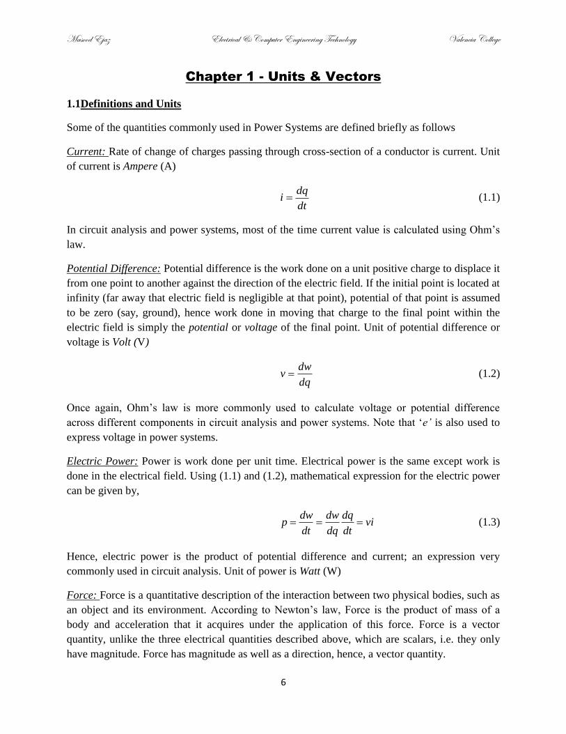
Magnetic Flux: The number of magnetic field lines (also considered as magnetic flux density)
passing through a surface. Magnetic flux is a scalar quantity which is the scalar or dot product
between the magnetic flux density vector and vector representing the area of the surface (a vector
perpendicular to the surface with magnitude as the area of the surface), as shown in figure 1.2
Figure 1.2: Magnetic Flux Density (B) crossing a surface area (A)
Mathematically, magnetic flux can be given by,
cos( )BA B.A (1.7)
where cos( )B is the component of magnetic flux density perpendicular to the surface or parallel
to the surface vector. If B is passing through the surface perpendicularly such that θ is 0o,
magnetic flux will be maximum and will be given simply by BA. Unit of magnetic flux is Weber
(Wb).
Magnetic Flux Density: Magnetic Flux Density (B) is simply number of magnetic lines per unit
area. It is a vector quantity. Unit of Magnetic Flux Density is Tesla (T) which is equal to Wb/m2.
Magnetic flux density will later be defined in terms of Magnetic Field Strength; a relationship
widely used in electromagnetism to characterize magnetic materials.
1.2 Per Unit System
Standard system of measurement is The International System of Units (SI) system. However,
there are other systems widely in use throughout the world and especially in U.S. Per Unit
System is a comparative way to express values of different quantities. Advantage of using per
unit system is that one can calculate the actual value of any quantity, expressed in per unit, in the
desired system if the reference or base value of the quantity is known in that system.
Per Unit value of any variable can be calculated by taking the ratio of that variable with the base
or reference value of the variable.

Masood Ejaz Electrical & Computer Engineering Technology Valencia College
9
( )base
XX pu
X (1.8)
Base value of a variable can also be found out from the base values of other variables from its
relationship formula with those variables.
1.3 Vector Arithmetic
Any vector in space can be defined in Rectangular or Cartesian form by breaking it down into its
components along with the three axes in space, as shown in figure 1.3.
Figure 1.3: Green vector is broken down into its components along with the three axes
Example 1.1
If base value of voltage is 100V, what will be the per unit value of 20KV voltage?
20( ) 200
100base
V KV pu pu
V
Example 1.2
If base value of voltage is 100V and base current is 10A, calculate the per unit value of
200Ω resistor.
10010
10
200( ) 20
10
basebase
base
base
VR
I
RR pu pu
R

Masood Ejaz Electrical & Computer Engineering Technology Valencia College
10
Hence, any vector A can be given in Cartesian coordinates as x y za a a A i j k , where ax, ay,
and az are the magnitudes of the vector along x, y, and z axes, and i, j, and k are the unit vectors
along the three axes. A unit vector is used to represent direction of a vector. A unit vector has
unity magnitude and its direction represents direction along the axis. Hence, unit vector i has
unity magnitude with direction along x-axis. Same goes for unit vectors j and k, as shown in
figure 1.
Figure 1.4: Unit vectors representing three axes
Note that throughout this text, we will be using the coordinate system as referenced in figure 1.4.
Dot Product: Dot product or scalar product is the product between two vectors that yields a
scalar quantity.
. cos( )c AB A B (1.9)
where A and B are the magnitudes of the two vectors A and B, and θ is the angle between them.
Note that since i, j, and k are perpendicular to each other, hence, anytime a dot product is carried
out between them, it will result in zero (cos(90o) = 0). Likewise, if a dot product is carried out
between two vectors parallel to each other, say ai and bi, it will simply be ab as cos(0) is unity.
Dot product is a commutative process, i.e. A.B = B.A
Example 1.3
Let 4 5 6 A i j k and 7 3 9 B i j k , calculate A.B
A.B = (4i+5j+6k).(7i+3j+9k) = 4i. 7i + 4i. 3j + 4i. 9k + 5j. 7i + 5j. 3j + 5j. 9k + 6k. 7i + 6k. 3j + 6k. 9k
→ A.B = 28+0+0+0+15+0+0+0+54 = 97
Note that A.B is a scalar quantity.

Masood Ejaz Electrical & Computer Engineering Technology Valencia College
11
Cross Product: Cross product is the product between two vectors that yields a vector quantity.
The resultant vector is perpendicular to both the vectors that were involved in the cross product.
sin( )AB C A B c (1.10)
where sin( )AB is the magnitude of vector C and c is a unit vector which is perpendicular to both
A and B. Note that if the two vectors are parallel to each other, the angle θbetween them will be
zero and magnitude of the resultant cross product vector will be zero as well. Also, if the two
vectors are perpendicular to each other, magnitude of the resultant cross product vector will be
maximum (AB) and direction will be perpendicular to both of the vectors.
When cross product between two different unit axes vectors is taken, it results in a unit vector
along the third axes, as shown in the table below.
Going Counterclockwise Going Clockwise
i × j = k i × k = -j
j × k = i k × j = -i
k × i = j j × i = -k
As discussed earlier, a cross product between same unit axes vectors will result in zero, as they
will be parallel to each other.
Keep in mind that cross product between two vectors A×B is not equal to B×A. Hence, cross product is
not a commutative operation.
Example 1.4
Let 4 5 6 A i j k and 7 3 9 B i j k , calculate A×B
A×B = (4i+5j+6k)×(7i+3j+9k) = 4i×7i + 4i×3j + 4i×9k + 5j×7i + 5j×3j + 5j×9k + 6k×7i + 6k×3j + 6k×9k
→A×B = 0+12k -36j -35k + 0 + 45i + 42j – 18i + 0 = 27i+6j-23k
Note that A×B is a vector quantity.

Masood Ejaz Electrical & Computer Engineering Technology Valencia College
12
PROBLEMS
1. Three resistors have the following ratings:
Resistor Resistance Power
A 100Ω 24W
B 50Ω 75W
C 300Ω 40W
Use resistor A as your base, determine the per-unit values of resistance, power, and voltage
rating of resistors B and C
2. Given flux density B = 4i + 6j + 7k wb/m2over cross-sectional area of a surface given by A =
2i + 8k m2, find the total flux crossing the surface.
3. Three vectors are given as follows:
A = 4i + 5j – 6k
B = 9i + 2j + 6k
C = 8i + 9k
Calculate: A×(B×C); (A×B)×C; A.(B×C); (A×B).C

Masood Ejaz Electrical & Computer Engineering Technology Valencia College
13
Chapter 2–Electricity & Magnetism
2.1 Fourier Series Discussion
In power systems and several other engineering fields, one encounters several types of periodic
waveforms. Many times these waveforms are sinusoidal but due to the addition of noise and
interference, they get distorted and become sinusoidal-like periodic waveforms. Many times they
are not like sinusoidal waveforms at all. For example, square waveforms, saw-tooth waveforms,
triangular waveforms etc. Fourier theory explains that any non-sinusoidal periodic waveform is a
combination of three components:
(i) An average or DC component, which is non-zero if waveform has unequal areas above
and below horizontal axis.
(ii) A sinusoidal component with same frequency as the frequency of the non-sinusoidal
waveform. This component is called fundamental component.
(iii) A number of sinusoidal components with frequencies that are multiple of the
fundamental frequency. These components are called harmonics.
According to Fourier theory, when the above three components are added together in an infinite
series, the original non-sinusoidal signal can be acquired. Mathematical expression of
trigonometric Fourier series is given as follows:
1
( ) cos( ) sin( )o n o n o
n
x t a a n t b n t
(2.1)
where ao is the average value of the non-periodic signal x(t), n is the harmonic number, ωo is the
frequency of signal x(t), and an and bn are the coefficients of harmonics. Note that fundamental
component is the first harmonic, i.e. n = 1 when the frequency of sinusoidal components is equal
to ωo.
As the number of harmonic increases in Fourier series, it’s contribution towards the non-
sinusoidal signal decreases, i.e. it’s amplitude becomes smaller and smaller. Practically, the non-
sinusoidal periodic signal may be achieved if the infinite series shown is (2.1) is truncated up to
the harmonic when the coefficients (amplitude) become small enough to be neglected.
Fourier series of a square waveform is given by the following expression,
1,3,5,7...
2( ) sin(2 )
2
p p
o
n
V Vv t nf t
n
(2.2)
Assume that the peak voltage is 10V and frequency of the signal is 100Hz, if we determine the
signal from (2.2) up to a specific harmonic, we will get the results as shown in figure 2.1.
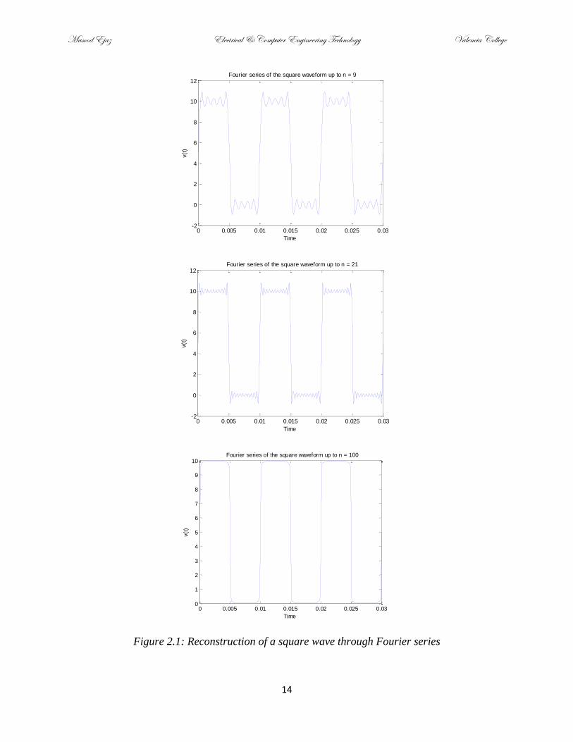
Masood Ejaz Electrical & Computer Engineering Technology Valencia College
14
Figure 2.1: Reconstruction of a square wave through Fourier series
0 0.005 0.01 0.015 0.02 0.025 0.03-2
0
2
4
6
8
10
12
Time
v(t
)
Fourier series of the square waveform up to n = 9
0 0.005 0.01 0.015 0.02 0.025 0.03-2
0
2
4
6
8
10
12
Time
v(t
)
Fourier series of the square waveform up to n = 21
0 0.005 0.01 0.015 0.02 0.025 0.030
1
2
3
4
5
6
7
8
9
10
Time
v(t
)
Fourier series of the square waveform up to n = 100

Masood Ejaz Electrical & Computer Engineering Technology Valencia College
15
2.2 Faraday’s Law of Electromagnetic Induction
Faraday’s law of electromagnetic inductions states that if a time varying flux is linking a coil
(inductor), a voltage is induced in the coil. This voltage is directly proportional to the rate of
change of flux.
ind
ind
de
dt
de N
dt
(2.3)
where constant of proportionality N is the number of turns of the coil. Observe the negative sign
in (2.3). This sign is in accordance with Lenz’s law that states that the direction of induced
voltage in the coil is such that if coil is short-circuited, it will run a current in the coil that will
produce a flux such that it will oppose the original flux that induced the voltage in the coil.
Note that if difference in flux is used instead of differential, (2.3) can be given by,
ind
ind
et
e Nt
(2.4)
Faraday’s law of electromagnetic induction is the basis of electric generators.
Example 2.1
A sinusoidal voltage signal is affected by interference and becomes non-sinusoidal due to
the inclusion of harmonics. If the 13th
harmonic has frequency of 223Hz, what will be the
frequency of the fundamental component of the signal?
13th
harmonic frequency = 13fofo= 223/13 = 17.15Hz
Example 2.2
A coil with 10 turns is linked with alternating flux given by ( ) 100cos(2000 )t t mWb.
Calculate the magnitude of induced voltage in the coil at t = 23ms.
23| | | | 10(0.1)(2000 )sin(2000 ) |ind t ms
de N t
dt
80.03pV

Masood Ejaz Electrical & Computer Engineering Technology Valencia College
16
2.3 Voltage Induced in a Moving Conductor
If magnetic field is stationary but a conductor is moving such that it is cutting the field, the coil is
experiencing a variable magnetic field across it. According to Faraday’s law, a voltage will be
induced in the coil. This voltage will depend on magnetic flux density, velocity of movement,
length of conductor experiencing the linkage of flux, and it can be given by the following
formula:
inde l.(v×B) (2.5)
where B is the flux density, v is the velocity, and l is the length vector. Length vector is assumed
to be positive in the direction of the flow of current.
For maximum induced voltage, velocity and magnetic flux density should be perpendicular to
each other, which will produce their cross product vector parallel to the length vector. In that
case induced voltage will simply be Blv.
inde lvB (2.6)
Example 2.3
A coil with 10 turns is linked with a constant flux of 10mWb through a DC magnet. The DC
magnet is now moved such that the new flux is 23mWb. It took 10ms for the flux to go from
10mWb to 23mWb. Calculate the magnitude of average voltage induced in the coil.
(23 10 )| | | | 10 13
10ind
m me N
t m
V
Example 2.4
A conductor is moving in space with velocity 3i+5j+7km/s and is placed parallel to x-axis. If
length of the conductor is 1.2m and the whole length is cutting the magnetic flux given by
4i+8kT, calculate the induced voltage and its direction in the conductor.
Assume that current is going to flow in the positive x direction, hence length vector can be
taken as 1.2i m.
eind = 1.2i . (3i+5j+7k × 4i+8k) = 1.2i . (-24j-20k+40i+28j) = 48V
Note that since our assumed direction of current is valid, induced voltage will be positive
along positive x-axis with respect to the other side.

Masood Ejaz Electrical & Computer Engineering Technology Valencia College
17
2.4 Lorentz Force
If a current carrying conductor is placed in magnetic field, it experiences a force. This force is
called Electromagnetic or Lorentz force. Mathematically, this force can be given by,
IF (l×B) (2.6)
where I is the current in the conductor, l is the length vector of the conductor taken positive in
the direction of the flow of current, and B is the magnetic flux density vector. Observe that the
force will be maximum when length vector and magnetic flux density are perpendicular to each
other. In that case magnitude of force will simply be given by,
F IlB (2.7)
Lorentz force is the basis of the working principle behind electric motors. Although direction of
Lorentz force may easily be found from (2.6), there is also a commonly used method called
right-hand rule to predict the direction of Lorentz force. According to this method, if index
finger of the right hand points towards the flow of current, i.e. direction of vector l and middle
finger points towards the magnetic flux density vector then thumb will point towards the
direction of force, as shown in figure 2.2.
Figure 2.2: Finding direction of Lorentz force using right-hand rule
Masood Ejaz Electrical & Computer Engineering Technology Valencia College
18
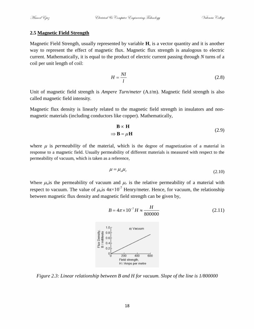
2.5 Magnetic Field Strength
Magnetic Field Strength, usually represented by variable H, is a vector quantity and it is another
way to represent the effect of magnetic flux. Magnetic flux strength is analogous to electric
current. Mathematically, it is equal to the product of electric current passing through N turns of a
coil per unit length of coil:
NIH
l (2.8)
Unit of magnetic field strength is Ampere Turn/meter (A.t/m). Magnetic field strength is also
called magnetic field intensity.
Magnetic flux density is linearly related to the magnetic field strength in insulators and non-
magnetic materials (including conductors like copper). Mathematically,
B H
B H (2.9)
where is permeability of the material, which is the degree of magnetization of a material in
response to a magnetic field. Usually permeability of different materials is measured with respect to the
permeability of vacuum, which is taken as a reference,
o r (2.10)
Where ois the permeability of vacuum and r is the relative permeability of a material with
respect to vacuum. The value of ois 4π×10-7
Henry/meter. Hence, for vacuum, the relationship
between magnetic flux density and magnetic field strength can be given by,
74 10800000
HB H (2.11)
Figure 2.3: Linear relationship between B and H for vacuum. Slope of the line is 1/800000

Masood Ejaz Electrical & Computer Engineering Technology Valencia College
19
For other non-magnetic materials (rubber, paper, copper etc.), relationship between B and H is
also linear with constant values for relative permeability, hence, different slope for the straight
line shown in figure 2.3. The linear relationship shows that the material can never be fully
magnetized, i.e. the north and south poles will never be fully aligned in the material.
For ferromagnetic and magnetic materials that can be fully magnetized, the relationship between
B and H can still be given by (2.9) and (2.10), i.e.
o rB H (2.12)
However, relative permeability is not constant and it changes as magnetic field strength increases
and material becomes more and more magnetized. B-H curves for different materials are shown
in figure 2.4
Figure 2.4: B-H relationship for different materials
Observe that while curve for air is linear (constant r), curves for iron and steel are not linear
and they saturate (magnetize) for higher values of H (variable r). The value of rmay still be
calculated using (2.12)

Masood Ejaz Electrical & Computer Engineering Technology Valencia College
20
2.6 Hysteresis Loop and Hysteresis Loss
When H increases due to flow of current in a magnetic or ferromagnetic material, magnetic poles
start aligning and B increases. If current keeps on increasing, magnetic flux density saturates (all
poles are aligned) as shown in figure 2.4. If the current that is producing the magnetic field is
removed, one will assume that the curve will go back to origin and all the poles will be
misaligned, leaving no magnetic flux in the material. However, this is not the case. Even when
the current is removed and H goes down to zero, there is still some magnetism left in the
magnetic material, as shown in figure 2.5.
Figure 2.5: Hysteresis Loop
Example 2.5
Use figure 2.4 to calculate the relative permeability for iron at 5000 At/m.
At H = 5000 At/m, B = 0.6T, hence, relative permeability will be,
80000096r
o
B B
H H
H/m
Hence, iron is 96 times more permeable than vacuum at H = 5000 At/m

Masood Ejaz Electrical & Computer Engineering Technology Valencia College
21
As it can be seen from figure 2.5, point a is the saturation point when current is increased and in
turn magnetic field strength is increased, when H goes to zero, B doesn’t go down to zero, it goes
to point b. This shows that there is still some residual flux (Br) left in the magnet (this property,
retentivity, is used in shunt generators and motors). To misalign all the magnetic poles and to
make the magnet neutral again, current needs to be supplied in the opposite direction, which will
change the direction of H and finally B will go down to zero at point c. The magnetizing force
required to make the magnet neutral again is called coercive force, Hc. If magnetic field strength
keeps on increasing in the opposite direction, magnet will saturate in quadrant 3, as shown in the
figure. Once again, when H goes to zero (current goes to zero), there is some residual flux left in
magnet in the opposite direction (point e). To make the magnet neutral again, coercive force is
required in the opposite direction, which is equal to the value of H at point f. If H keeps on
increasing, magnet will again saturate and will go to point a, hence completing the loop. This
loop is called Hysteresis loop and it is very commonly used to understand the magnetizing
characteristics (retentivity, coercivity etc.) of a material. Figure 2.6 shows the hysteresis loop in
a bit more detail.
Figure 2.6: Hysteresis loop with details

Masood Ejaz Electrical & Computer Engineering Technology Valencia College
22
In most of the electric machines including motors, generators, transformers etc., there is AC
current that changes its direction. Most of the machines have their cores on which coils are
wounded made out of ferromagnetic or magnetic materials. When current flows in these coils, it
sets up a magnetic field in the core. Since current is alternating, magnetic field is also alternating
and it can be defined by hysteresis loop. Since energy is required to set up a magnetic field and
to keep changing the direction of magnetic field in the core, this energy heats up the core. This
loss of energy in terms of heat is called hysteresis loss. To reduce hysteresis losses, cores of AC
machines and equipment are made of materials with narrow hysteresis loops.
2.7 Eddy Currents
If an AC flux is linked with a loop of conductor, voltage is induced in it per Faraday’s law. If the
coil is short-circuited, an alternating current will flow through it producing heat due to coil
resistance. Likewise, if another coil is placed inside the first coil, it will interact with less flux;
hence, smaller voltage will induce in it which will circulate smaller amount of current if it is
short-circuited as well. This scheme can be repeated several times to get circular patterns of
short-circuited currents producing substantial amount of heat, as shown in figure 2.7
Figure 2.7: Currents revolving around short circuit loops due to induced voltages
Now consider a metal plate linked with an alternating flux. This metal plate may be considered
as many short-circuit loops one inside another. Therefore, an alternating flux will induce
voltages in the metallic plate which will result in the establishment of circular current paths, as
shown in figure 2.8. These currents are called Eddy currents and they result in producing
substantial amount of heat in metallic components linked with alternating flux.

Masood Ejaz Electrical & Computer Engineering Technology Valencia College
23
Figure 2.8: Eddy Currents
This poses a serious problem in AC motors, generators and transformers; AC flux produced due
to the flow of AC current in the coils is linked with the core and other metallic parts of the
machine, inducing voltage and producing Eddy currents. This result in heating of the core,
termed as Eddy current loss, and may reduce performance of the machine as well as its life.
To alleviate this problem up to great extent, all the AC machines have cores made out of
laminated sheets of metal which are insulated from each other, as shown in figure 2.9. This
arrangement results in small induced voltages in each laminated sheet, which produce very small
Eddy currents in each lamination. These small Eddy currents produce extremely small Eddy
current loss in each lamination and even their cumulative effect is only a fraction of loss occurs
in non-laminated core.
Figure 2.9: Laminated core of electric machine

Masood Ejaz Electrical & Computer Engineering Technology Valencia College
24
PROBLEMS
1. B-H curves of steel, iron and air are given in figure 2.4. Find the value of relative
permeability of steel and iron at H = 3000 At/m.
2. If a time varying flux given by is linking a coil with 100 turns, what will be
the magnitude of voltage in the coil at t = 2s?
3. If a conductor is cutting a magnetic field with B = 4i+ 5kwb/m2and velocity of rotation at a
certain time can be given by v = 2i + 3jm/s, what will the value of induced voltage if length
of the conductor is 1.5 m and it is placed along x-axis? If you short-circuit the conductor, in
which direction current is going to flow through it?
4. If a current carrying conductor is placed in the magnetic field as shown in figure 2.10, what
will be the magnitude and direction of the force it will experience?
Figure 2.10: Current Carrying Conductor in a Magnetic Field
5. A single conductor is rotating counter clockwise around the axis as shown in figure 2.11.
Magnitude of rotation velocity is 2m/s. How much voltage will be induced at the ends of
conductor (ab) if position of conductor is as shown in the figure? Also mention what will be
the polarity of the two ends.
(Hint: use equation E = (v x B).l and calculate voltage on each side before adding them
together)
B = 1.2 mWb/m2
I = 2A
l = 5m

Masood Ejaz Electrical & Computer Engineering Technology Valencia College
25
Figure 2.11: A single loop rotating inside a magnetic field

Masood Ejaz Electrical & Computer Engineering Technology Valencia College
26
Chapter 4 – Direct-Current Generators
4.1 Principle of Generator Operation
Electrical generators are operated on the principle of Faraday’s law, i.e. if a loop of wire is linked
with time-varying magnetic flux, a voltage will be induced in the coil. If a load is connected to
the terminals of the coil, this induced voltage will drive a current through the load. Based on this
explanation, observe the arrangement of basic electric generator in figure 4.1.
Figure 4.1: Basic Alternator (A.C. Generator)
As it can be seen in figure 4.1, different parts of the generator are magnets to produce magnetic
field, a coil that is rotating in the magnetic field in which voltage will be induced, two slip rings
where individual conductors from each end of the coil are connected, and two carbon brushes
that carry current to the load. The assembly of the coil where voltage is induced in the machine is
called armature. Most of the machines have rotating armature but there are some machines
where magnetic field is rotating and armature is stationary.
To understand how the voltage will be induced in the coil, observe that magnetic field B on the
coil is from left to right (j direction), assume that axis of rotation is right in the middle of the coil
along x-axis, the left half of the coil (red) will have velocity vector going downwards (-k
direction) and the right half (blue) will be going upward (k direction). The voltage induced on
the side under North Pole of the magnet (AB)will be along positive x direction [eind = l.(v×B) =
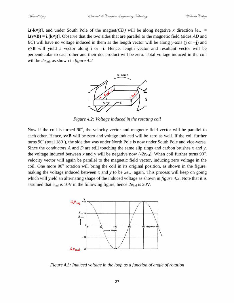
Masood Ejaz Electrical & Computer Engineering Technology Valencia College
27
i.(-k×j)], and under South Pole of the magnet(CD) will be along negative x direction [eind =
l.(v×B) = i.(k×j)]. Observe that the two sides that are parallel to the magnetic field (sides AD and
BC) will have no voltage induced in them as the length vector will be along y-axis (j or –j) and
v×B will yield a vector along i or –i. Hence, length vector and resultant vector will be
perpendicular to each other and their dot product will be zero. Total voltage induced in the coil
will be 2eind, as shown in figure 4.2
Figure 4.2: Voltage induced in the rotating coil
Now if the coil is turned 90o, the velocity vector and magnetic field vector will be parallel to
each other. Hence, v×B will be zero and voltage induced will be zero as well. If the coil further
turns 90o (total 180
o), the side that was under North Pole is now under South Pole and vice-versa.
Since the conductors A and D are still touching the same slip rings and carbon brushes x and y,
the voltage induced between x and y will be negative now (-2eind). When coil further turns 90o,
velocity vector will again be parallel to the magnetic field vector, inducing zero voltage in the
coil. One more 90o rotation will bring the coil in its original position, as shown in the figure,
making the voltage induced between x and y to be 2eind again. This process will keep on going
which will yield an alternating shape of the induced voltage as shown in figure 4.3. Note that it is
assumed that eind is 10V in the following figure, hence 2eind is 20V.
Figure 4.3: Induced voltage in the loop as a function of angle of rotation

Masood Ejaz Electrical & Computer Engineering Technology Valencia College
28
Figure 4.4 shows induced voltage plot against time assuming speed of rotation to be 60 rpm.
There will be one rotation per second giving frequency of the rotation to be 1Hz and time period
of the waveform to be 1 second.
Figure 4.3: Induced voltage in the loop as a function of time
Note that the basic generator does not always produce a pure sinusoidal voltage as shown in the
above figures. The shape of the output voltage depends upon the shape and enclosure of the
magnets. If properly designed, shape will be very close to sinusoid else there will be harmonics
in the induced voltage. For the sake of simplicity, for our study, most of the time we will assume
a sinusoidal induced voltage.
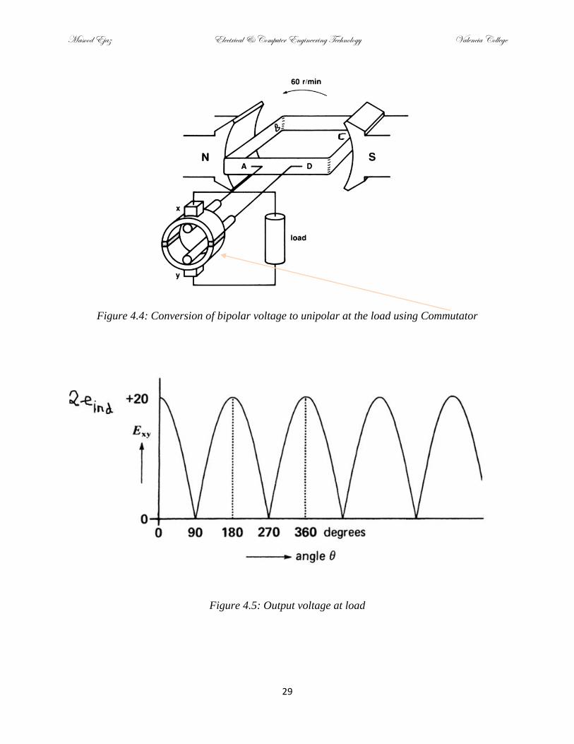
4.2 Commutation Process
As explained in the previous section, the natural shape of the induced voltage in a rotating coil is
bipolar, i.e. a coil rotating in a magnetic field will always have an AC voltage induced between
its terminals. To get a unipolar (DC) voltage, a special arrangement is done at the terminals as
shown in figure 4.4. The two slip rings are replaced by a single one which is split in two halves
insulated from each other. This is called a commutator. The two carbon brushes are touching the
two halves of the commutator. As the coil moves, the commutator halves keep switching
between the two carbon brushes instead of touching the same one as it was the case with the
arrangement shown in figure 4.1 that produced AC voltage at the load. Now when the coil AB is
under the North Pole, it will be touching the top brush x, and once it will move to the other side
(under South Pole), it will be touching the bottom brush y. At this time coil CD will be under
North Pole touching the top brush x. Hence, the voltage at brush x will always be positive with
respect to brush y throughout the course of rotation and load voltage will be DC Pulsating as
shown in figure 4.5.
Masood Ejaz Electrical & Computer Engineering Technology Valencia College
29
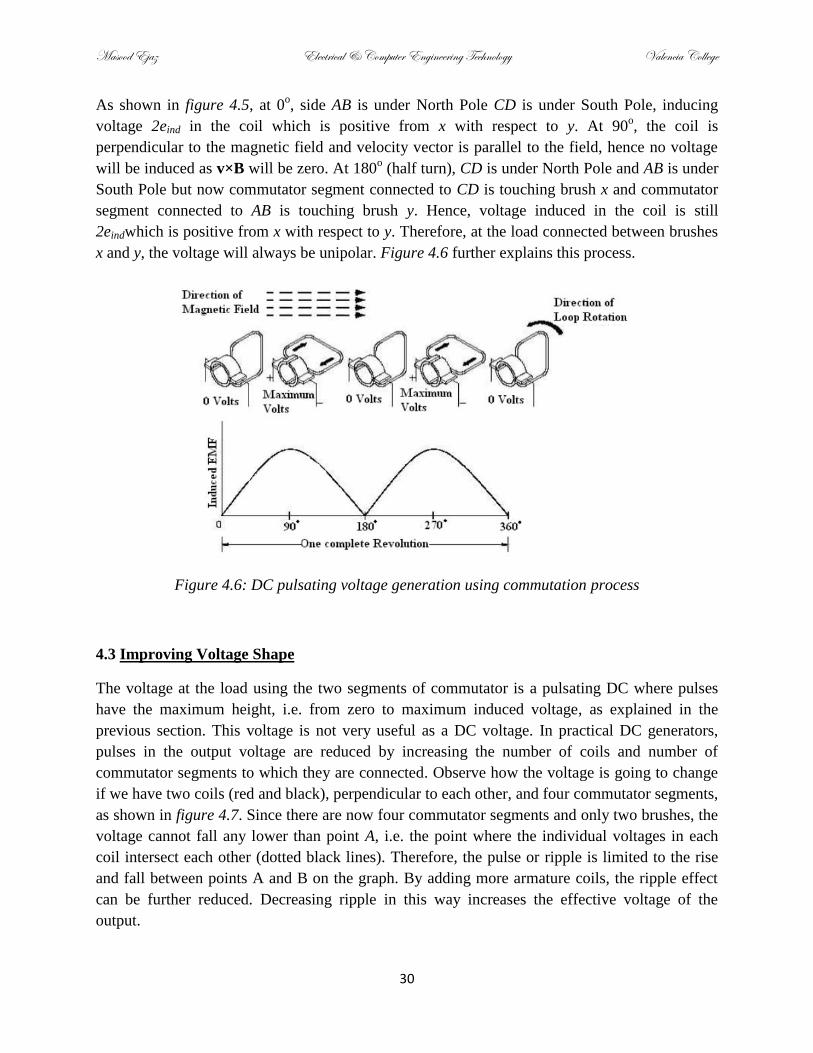
Figure 4.4: Conversion of bipolar voltage to unipolar at the load using Commutator
Figure 4.5: Output voltage at load
Masood Ejaz Electrical & Computer Engineering Technology Valencia College
30
As shown in figure 4.5, at 0o, side AB is under North Pole CD is under South Pole, inducing
voltage 2eind in the coil which is positive from x with respect to y. At 90o, the coil is
perpendicular to the magnetic field and velocity vector is parallel to the field, hence no voltage
will be induced as v×B will be zero. At 180o (half turn), CD is under North Pole and AB is under
South Pole but now commutator segment connected to CD is touching brush x and commutator
segment connected to AB is touching brush y. Hence, voltage induced in the coil is still
2eindwhich is positive from x with respect to y. Therefore, at the load connected between brushes
x and y, the voltage will always be unipolar. Figure 4.6 further explains this process.
Figure 4.6: DC pulsating voltage generation using commutation process
4.3 Improving Voltage Shape
The voltage at the load using the two segments of commutator is a pulsating DC where pulses
have the maximum height, i.e. from zero to maximum induced voltage, as explained in the
previous section. This voltage is not very useful as a DC voltage. In practical DC generators,
pulses in the output voltage are reduced by increasing the number of coils and number of
commutator segments to which they are connected. Observe how the voltage is going to change
if we have two coils (red and black), perpendicular to each other, and four commutator segments,
as shown in figure 4.7. Since there are now four commutator segments and only two brushes, the
voltage cannot fall any lower than point A, i.e. the point where the individual voltages in each
coil intersect each other (dotted black lines). Therefore, the pulse or ripple is limited to the rise
and fall between points A and B on the graph. By adding more armature coils, the ripple effect
can be further reduced. Decreasing ripple in this way increases the effective voltage of the
output.

Masood Ejaz Electrical & Computer Engineering Technology Valencia College
31
Figure 4.7: Ripple reduction at the terminal with more coils and commutator segments
By using additional armature coils, the voltage across the brushes is not allowed to fall to as low
a level between peaks. Practical generators use many armature coils. They also use more than
one pair of magnetic poles. The additional magnetic poles have the same effect on ripple as did
the additional armature coils. In addition, the increased number of poles provides a stronger
magnetic field (greater number of flux lines). This, in turn, allows an increase in output voltage
because the coils cut more lines of flux per revolution.
4.4 Commutation in a Four Loop DC Generator
Most of the armatures have either same number of coils as the number of slots or more coils
fitted into lesser number of slots. Each coil can have multiple turns as well, and each turn or loop
has one conductor on each side, i.e. total two conductors for one turn. Observe in figure 4.8 how
four loops are fitted into four slots.

Masood Ejaz Electrical & Computer Engineering Technology Valencia College
32
Figure 4.8: An armature with four slots, four loops and four commutator segments
In figure 4.8, armature of DC machine is shown placed in between the permanent poles of a
magnet. Four loops with yellow, blue, green and orange color form armature winding and ends
of these loops are connected with the commutator of the machine. Outermost and innermost
wires of loops around the rotor are represented. The commutator is touching the carbon brushes
and direction of rotation is such that polarities of brushes are ‘+’ and ‘-‘, as shown.
Consider figure 4.8 in 2-D at moment ωt=0 in figure 4.9. Four loops are shown with red, yellow,
blue and orange color. The outermost wires of every loop are labeled with numbers 1, 2, 3 and 4,
whereas innermost wire is labeled with prime over a number, i.e. 1′, 2′, 3′ and 4′. a, b, c and d
represent four commutator segments.
Figure 4.9: 2-D image of armature with four slots, four coils, and four armature slots

Masood Ejaz Electrical & Computer Engineering Technology Valencia College
33
Observe that the outermost wire of the blue loop (2) is connected to commutator segment a,
whereas innermost wire (2’) is connected to b. Similarly outermost wire of the orange coil (4) is
connected to c, whereas innermost wire (4’) is connected to segment d. Red wire, 1 and 1′, are
connected to b and c, whereas yellow wire, 3 and 3′, are connected to d and arespectively.Now if
we draw the armature windings from figure 4.9 in 2-D then the polarity over segments is due to
connections with brushes, as shown in figure 4.10.
Figure 4.10: Armature coil arrangement in 2-D
Observe from figure 4.9 that wire terminals 1,3′,2 and 4′ are under magnetic force of the North
Pole, whereas 1′,3, 2′ and 4 ends are under magnetic force of the South Pole.
Assume that each loop has a voltage contribution of e. In the present case, all four loops are lying
within poles so overall voltage is Eind =4e between brushes a andb.
Now assume that the armature is rotated counter clockwise by 45o. Now the blue and orange
loops are not facing any magnetic force, whereas red and yellow loops are under magnetic force,
as shown in figure 4.11.
Figure 4.11: Armature rotated counter clockwise by 45o

Masood Ejaz Electrical & Computer Engineering Technology Valencia College
34
No voltage will be induced in coils 2 (blue) and 4 (orange) at this time and voltage e will be
induced in each of the conductor of loop 1 (red) and 3 (yellow), as shown in figure 4.12.
4.12: Voltage induced in the armature coil rotated to 45o
Notice that at this instant brushes of the machine are shorting out commutator segments ab and
cd. This happens just at the time when the loops between these segments have 0V across them,
so shorting out the segments creates no problem. At this time only loops 1 and 3 are under the
pole faces, so the terminal voltage will be 2e.
Now if the armature is rotated counter clockwise by 45o again, i.e. total 90
o, it will look like the
one shown in figure 4.13.
Figure 4.13: Armature rotated counter clockwise by 90o

Masood Ejaz Electrical & Computer Engineering Technology Valencia College
35
The voltage induced between the brushes will again be 4e, as shown in figure 4.14.
Figure 4.14: Voltage induced in the armature coil rotated to 90o
Note that the output voltage shape is similar to the one shown in figure 4.7 except the amplitude
has increased. This is due to the fact that number of coils has increased in the slots.
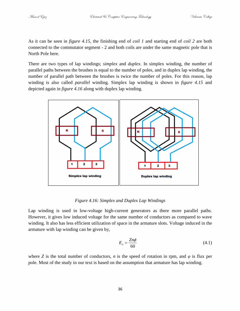
4.5 Types of Armature Winding
The two most common types of armature winding are lap winding and wave winding.
Lap Winding
Lap winding is the winding in which successive coils overlap each other. It is named "Lap"
winding because it doubles or laps back with its succeeding coils. In this winding the finishing
end of one coil is connected to one commutator segment and the starting end of the next coil,
situated under the same pole, is connected to the same commutator segment, as shown in figure
4.15
Figure 4.15: Lap Winding
Masood Ejaz Electrical & Computer Engineering Technology Valencia College
36
As it can be seen in figure 4.15, the finishing end of coil 1 and starting end of coil 2 are both
connected to the commutator segment - 2 and both coils are under the same magnetic pole that is
North Pole here.
There are two types of lap windings; simplex and duplex. In simplex winding, the number of
parallel paths between the brushes is equal to the number of poles, and in duplex lap winding, the
number of parallel path between the brushes is twice the number of poles. For this reason, lap
winding is also called parallel winding. Simplex lap winding is shown in figure 4.15 and
depicted again in figure 4.16 along with duplex lap winding.
Figure 4.16: Simplex and Duplex Lap Windings
Lap winding is used in low-voltage high-current generators as there more parallel paths.
However, it gives low induced voltage for the same number of conductors as compared to wave
winding. It also has less efficient utilization of space in the armature slots. Voltage induced in the
armature with lap winding can be given by,
60o
ZnE
(4.1)
where Z is the total number of conductors, n is the speed of rotation in rpm, and φ is flux per
pole. Most of the study in our text is based on the assumption that armature has lap winding.

Masood Ejaz Electrical & Computer Engineering Technology Valencia College
37
Wave Winding
In wave winding, the end of one coil is connected to the starting of another coil such that all the
coils carrying current in the same direction are connected in series i.e., coils carrying current in
one direction are connected in one series circuit and coils carrying current in the opposite
direction are connected in other series circuit. This is why wave winding is also called series
winding. Wave winding is shown in figure 4.17
Figure 4.17: Wave Winding
If after passing once around the armature the winding falls in a slot to the left of its starting point
then winding is said to be retrogressive. If it falls one slot to the right, it is progressive. Both
types are shown in figure 4.18
Figure 4.18: Types of Wave Winding
Progressive
Retrogressive

Masood Ejaz Electrical & Computer Engineering Technology Valencia College
38
Wave winding is used for low-current high-voltage machines. Both lap and wave windings in an
armature are shown in figure 4.19
Figure 4.19: Lap and Wave Windings
4.6 Armature Reaction
Let’s take a step back and observe figure 4.12 once again where coil 2 is shorting commutator
segments a andb and coil 4 is shorting commutator segments c and d. Since coil 2 and coil 4 do
not have any induced voltage, hence, even if they short two commutator segments, it will not do
any harm to the brushes connected to those segments. If there would be some voltage induced in
those coils then there would be a lot of sparking at the brushes which lead to less than full
voltage available at the brushes and constant sparking also reduces the life of the brush. Hence, it
is very important to position the brushes on the armature such that if a coil shorts two
commutator segments that are touching the brush, voltage induced in those segments should
always be zero.
An armature with 12 coils and 12 commutator slots is shown in figure 4.20. Observe that the two
coils that are shorting the commutator segments touching the brushes, again, have zero induced
voltage as no flux is linking with them. The plane along which flux is zero is called neutral zone
or neutral plane and brushes are supposed to be placed on this plane as any coil on neutral zone
will have zero voltage induced in it, hence, eliminating the danger of brush sparking and reduced
output voltage.

Masood Ejaz Electrical & Computer Engineering Technology Valencia College
39
Figure 4.20: Output terminal voltage with brushes located along neutral zone
As shown in figure 4.20, induced voltage between the output terminals will be 70V
(7+18+20+18+7). If now we connect the brushes not along the neutral zone, as shown in figure
4.21, observe that the terminal voltage goes down to 63V. There will also be sparking at the
brushes as the two commutator segments touching the brushes are now shorted out by coils with
non-zero induced voltage in them.
Figure 4.21: Output terminal voltage when brushes are not located on neutral zone

Masood Ejaz Electrical & Computer Engineering Technology Valencia College
40
When a load is connected to the output terminals and current starts flowing in the armature, a
magnetic field is produced due to this flow of current. This is armature magnetic field producing
armature flux, as shown in figure 4.22. Note that ‘.’ represents current going into the page
whereas ‘+’ represents current coming out of the page.
Figure 4.22: Armature flux due to armature current
When armature flux interacts with field flux, the cumulative magnetic flux linking the coil is
changed. Now, it is quite possible that this cumulative flux is linking the coils along neutral zone
and some other coils are not linked with the flux at all. Hence, orientation of neutral zone is
changed, as shown in figure 4.23. Since brushes are still located along the original neutral zone
(neutral zone without any load connected), output voltage will be reduced and sparking will
occur at the brushes. This dislocation of neutral zone is called armature reaction that results in
reduced output voltage and brush sparking, which consequently reduces the life of brushes.
There are two ways to tackle armature reaction. The first one is to relocate the brushes along the
new neutral zone. This is a temporary fix as if generator load will change, armature current will
change and new cumulative flux will change the location of neutral zone.

Masood Ejaz Electrical & Computer Engineering Technology Valencia College
41
Figure 4.23: Dislocation of neutral zone
The second method, which is mostly used in practice, is to introduce commutating poles, as
shown in figure 4.24. Commutating poles are electromagnets that are wound by few turns of
thick wires and placed in series with armature winding and load. When current flows towards the
load, it passes through the commutating poles that produce their own magnetic flux which is
equal but opposite in direction to the armature flux. Hence, two fluxes cancel each other leaving
only the original field flux and neutral zone is not disturbed. This method of countering armature
reaction does not depend upon load current as armature flux and commutating poles flux will
always be equal and opposite, hence cancelling each other.
Figure 4.24: Commutating poles to tackle armature reaction

Masood Ejaz Electrical & Computer Engineering Technology Valencia College
42
4.7 Types of DC Generators
Depending on their field, DC generators can be divided into three categories:
i. Separately excited generators
ii. Shunt generators
iii. Compound generators
4.7.1 Separately Excited Generators
In separately excited generators, field is either produced by a permanent magnet or
electromagnet excited by a separate DC source. Hence, the field flux is constant and does not
depend upon the induced voltage. Figure 4.25 shows separately excited generator and its
equivalent circuit diagram.
Figure 4.25: Separately Excited Generator
When field is excited by the field current, flux increases linearly. As current keeps on increasing,
magnetic core of the field starts saturating and in turns field flux starts saturating. Usually the
current supplied to the field is such that the field flux just enters into saturation, as shown by the
knee of the flux vs. current curve in figure 4.26. Remember, if armature is turning at a constant
speed, more voltage will be induced if field flux will be higher, i.e. if field current will be higher.
If field flux is constant, turning the armature at a higher speed will induce more voltage as rate of
change of flux through armature coils will be higher.
To change the direction of induced voltage, direction of field flux may be reversed, i.e. field
current may be reversed by changing the polarity of field supply. Induced voltage direction may
also be changed if armature is turned in the opposite direction. If both field supply polarity and
direction of armature rotation is changed, induced voltage direction will not be changed.
(a) Physical Construction
(b) Equivalent Circuit Diagram

Masood Ejaz Electrical & Computer Engineering Technology Valencia College
43
Figure 4.26: Induced voltage vs. field current
No-load terminal voltage for separately excited generators is the same as induced voltage. When
a load is connected to the terminals and current starts flowing in the armature, terminal voltage
drops due to some drop in the armature resistance. For separately excited generators, no-load to
full-load terminal voltage drop is in the range of 5-10%
Example 4.1
A separately excited generator has lap-wound armature with 12 slots and 20 turns per coil. It
has two poles with flux per pole to be 100mWb. Armature is turning at 100 rpm. If armature
resistance is 1Ω and a 100 Ω load is connected to the terminals, calculate the terminal
voltage.
Since armature is lap-wound, induced voltage may be calculated as follows:
(12 20 / 2 / )(100)(100E 3)80
60 60
Zn coils turns coil conductors turnEo V
Using voltage division, terminal voltage may be calculated as follows:
79.20LT o
L o
RE E V
R R
Figure 4.27: Separately excited generator under load
Masood Ejaz Electrical & Computer Engineering Technology Valencia College
44
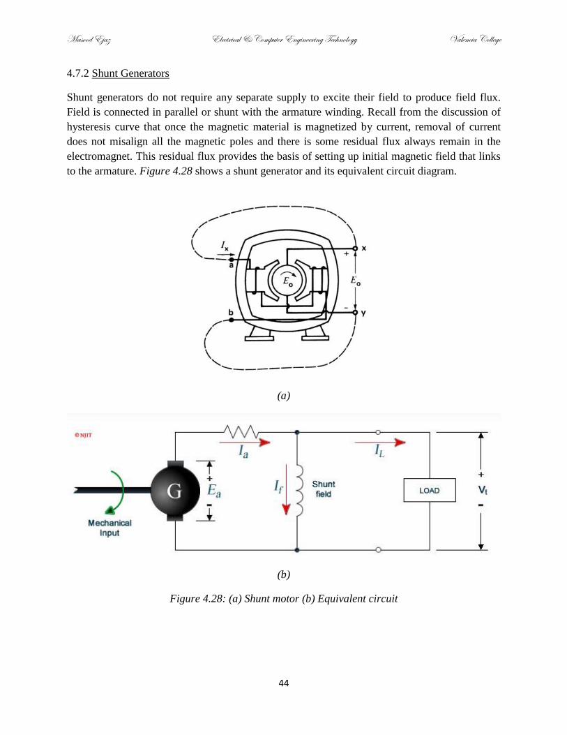
4.7.2 Shunt Generators
Shunt generators do not require any separate supply to excite their field to produce field flux.
Field is connected in parallel or shunt with the armature winding. Recall from the discussion of
hysteresis curve that once the magnetic material is magnetized by current, removal of current
does not misalign all the magnetic poles and there is some residual flux always remain in the
electromagnet. This residual flux provides the basis of setting up initial magnetic field that links
to the armature. Figure 4.28 shows a shunt generator and its equivalent circuit diagram.
(a)
(b)
Figure 4.28: (a) Shunt motor (b) Equivalent circuit

Masood Ejaz Electrical & Computer Engineering Technology Valencia College
45
Note that in figure 4.28, equivalent circuit of shunt motor has current Ia flowing through
armature resistance, If flowing through field resistance, and IL flowing through the load. Terminal
voltage is applied across the shunt field which is equal to the induced voltage minus the drop in
the armature resistance.
Working of the shunt motor can be explained as follows. When armature is rotated, it is linked
with the residual flux from the field winding. This small residual flux induces a small voltage in
the armature. This induced voltage runs a small current that goes to the field that increases the
amount of field flux, which in turns induces more voltage in the armature. Now relatively higher
voltage produces more current that goes to the field and produces higher flux, which in turns
produces even higher voltage. This cycle keeps on going until the induced voltage reaches to a
maximum value determined by the field resistance and degree of saturation.
Controlling the voltage of shunt generator:
A simple way to control the induced voltage of a shunt generator is to connect a rheostat
(variable resistor) in series with the field winding that can be used to control the field current and
in turn field flux that links to the armature coil, as shown in figure 4.29.
Figure 4.29: Rheostat field current control scheme for shunt generators
To control the field current, an initial value of rheostat is selected that produces flux to induce a
base voltage. If induced voltage below the base value is required, rheostat value may be
increased that will reduce the field current, hence, less flux will be produced that will lower
down the value of the induced voltage. Likewise, if value above the base value is required,
rheostat value will be reduced. This phenomenon is shown in the following graph between no-
load voltage and field current.

Masood Ejaz Electrical & Computer Engineering Technology Valencia College
46
Figure 4.29: Terminal voltage at no load versus field current
Observe that the straight lines represent the relationship between induced or terminal voltage
(neglect the small armature resistance) and field current using Ohm’s law (Eo = If(Rt+Rf)) and
curve represents the induced voltage per hysteresis phenomenon where increase in the field
current after saturation point will not increase the flux appreciably. The intersection of two
curves determine the value of the induced voltage or terminal voltage at no-load. Observe that if
the rheostat value will keep on increasing to reduce the amount of field current to reduce the
value of induced voltage, at one point the straight line will become tangent to the hysteresis
curve and will not intersect it. As soon as this will happen, induce voltage as well as terminal
voltage will go down to zero. Hence, the value of field rheostat has a maximum value beyond
which it cannot be increased.
Effect of the load on the terminal voltage:
In separately-excited generators, induced voltage is not changed by the load. However, terminal
voltage does change by the load as when current starts flowing in the armature, some voltage is
dropped in it and terminal voltage becomes smaller than the induced voltage. In shunt generators,
since field current also depends on the terminal voltage, as load increases and more current starts
flowing out of armature, terminal voltage drops. This in turns reduces the field current (If =
ET/Rf), which in turns reduces the field flux and induced voltage further goes down. The no-load
to full-load voltage in shunt generators is smaller than separately-excited generators. Generally,
full-load voltage of shunt generators is about 15% less than the no-load voltage.

Masood Ejaz Electrical & Computer Engineering Technology Valencia College
47
4.7.3 Compound Generators
Separately-excited generators require a separate source to excite the field. However, their
terminal voltage under load is greater than shunt generators that do not require a separate source
to excite their field. To have the benefit of self-excitation like shunt generators and higher
terminal voltage, compound generators are designed. In compound generators there are two filed
windings; one in parallel (shunt) and one in series with the load. The series winding is comprised
of few turns of thick wires that produces flux when current flows to the load. Depending on the
series field winding, compound generators can either be cumulative or differential.
Figure 4.30: (a) Compound generator (b) Equivalent circuit
Example 4.2:
Induced voltage of a shunt generator is 100V, terminal voltage is 90V, field resistance is
20Ω, and armature resistance is 1Ω. Calculate armature current, field current and load
current.
100 9010
1
904.5
20
10 4.5 5.5
A
f
load
I A
I A
I A

Masood Ejaz Electrical & Computer Engineering Technology Valencia College
48
When load current flows in the cumulative compound generators, the series field flux is
produced in the same direction as the shunt field flux, hence they are added together. This higher
flux induces higher voltage in the armature which in turns produces higher terminal voltage.
Hence the terminal voltage either drops a little bit under full load or may not drop at all. In
differential compound generators, series flux is in the direction opposite to the shunt flux, hence
total flux goes further down and induced voltage is even smaller which in turns produces smaller
terminal voltage. Due to this reason, differential generators do not find much practical use.
Example 4.3:
A cumulative compound generator has lap-wound armature with 100 slots, and 4 turns per
coil. It is rotation with a speed of 100rpm. Flux per pole is 100mWb. Series field resistance
is 2Ω and shunt field resistance is 100Ω, Armature resistance is 1Ω. Calculate:
(i) Induced Voltage:
Z = slots*turns_per_coil*conductors_per_turn = 800 conductors
Eo = Z*n*/60 = 133.33V
(ii) Terminal Voltage:
Ia = Eo/(Ra + Rshunt) = 1.3201A
Et = Eo - Ia*Ra = 132.01V
(iii) If a 100 load is connected to the terminals and it starts driving the current such that
series field starts producing 10mWb flux per pole and shunt flux per pole drops down to
85mWb, calculate the load power.
new = 95mWb
Eonew = Z*n*new /60 = 126.67V
Req =( Rseries+RL)||Rshunt = 50.495
Ianew = Eonew/(Req+Ra) = 2.4598A
Using current division:
IL = Ianew *Req/(RL + Rseries) = 1.2177A
Pload = IL2*RL = 148.28W

Masood Ejaz Electrical & Computer Engineering Technology Valencia College
49
4.8 Generator Specifications
Every generator has a nameplate with its ratings or nominal characteristics. These specifications
may tell us about the rated power, rated terminal voltage, type of machine, shunt field current,
speed of armature rotation for rated values, operable temperature, and insulation class. Load
current as well as series field current (in case of compound generator) can be calculated by
dividing the rated power by the terminal voltage. An example of generator nameplate is shown in
figure 4.31.
Power 100KW Speed 1200 rpm
Voltage 250V Type Compound
Exciting Current 20A Class B
Temperature Rise 50oC
Figure 4.31: A DC Generator Sample Nameplate
The nameplate tells us that generator can deliver 100KW power at 250V, without exceeding the
temperature rise of 50oC, when it rotates at the rated speed of 1200rpm. Hence, the maximum
load current that it can supply is 100K/250 = 400A. It is a compound motor with shunt field
current to be 20A. Series filed current depends on the load current but it cannot exceed 400A.
Class B is the insulation type that corresponds to the materials that withstand temperature up to
130oC.

Masood Ejaz Electrical & Computer Engineering Technology Valencia College
50
PROBLEMS
Note: Draw circuit for each problem.
1. A shunt generator has field resistor value Rf = 60and no –load induced voltage rating Eo =
220V. A 60 resistor is added in series to the field winding to reduce field current by 60%
and hence to reduce the maximum no-load generator induced voltage. What will be the new
value of the induced no-load voltage? Ignore armature resistance. (Note: Current is reduced
by 60% that means the new current is 40% of the original value.)
2. A compound generator has a lap-wound armature with 12 slots and 4 turns per coil. At no-
load, flux per pole is 0.5Wb and it is running at 900 rpm. Shunt resistance is 100series
filed resistance is 3, and armature resistance is 0.5.
(a) Calculate induced voltage, armature current and terminal voltage at no-load.
(b) If a 100 load is connected to the terminals and the series flux is added to the shunt flux
such that it remains the same as it was at no-load, calculate the terminal voltage, armature
current, and power dissipated in the load.
3. A separately excited generator has lap-wound armature with 12 slots and 5 turns per coil. It is
rotating at 300rpm. There are 6 poles and total flux linking the armature is 6 Wb. Armature
resistance is 2Ω. There is a 100Ω load connected to the terminals. Calculate:
(i) Induced voltage
(ii) Armature current
(iii) Terminal voltage
(iv) Power delivered to the load

Masood Ejaz Electrical & Computer Engineering Technology Valencia College
51
Chapter 5–Direct-Current Motors
5.1 Principle of Operation
Construction of DC motors is exactly like DC generators except load is replaced by a DC power
supply that supplies current to the armature. When this current is interacted with the field flux,
Lorentz force is acted upon the armature (rotor), which applies a torque on it and it starts rotating
about its axis. Figure 5.1 shows a basic DC motor.
Figure 5.1: A simple single loop DC motor
Observe that in figure 5.1, magnetic field is from right to left (-j). Since current is going into the
page (-i) under S-pole, force on that conductor will be in the direction of L×B, i.e. -i×-j = k, i.e.
upward. Likewise, the conductor under N-pole will experience a downward force. Therefore,
direction of rotation of the armature will be clockwise.
DC motors provide a very large starting torque, as will be discussed soon, and in general their
speed-torque characteristics can be varied over a wide range while maintaining high efficiency;
that’s why electric cars do not have any gears.
5.2 Counter-electromagnetic Force (CEMF)
As initial current flows in the armature and it is acted upon by the Lorentz force and starts
rotating, magnetic field interacting with the armature starts changing. This changing magnetic
field induces a voltage in the armature coils per Faraday’s law of electromagnetic induction.

Masood Ejaz Electrical & Computer Engineering Technology Valencia College
52
Observe from figure 5.1 that if the coil is rotating clockwise, the voltage induced in the
conductor (v×B) will k×-j = i, i.e. along positive x-axis under S-pole, and along negative x-axis
under N-pole. Therefore, the induced voltage is in the direction opposite to the applied voltage;
hence, it is called counter-electromotive force. Circuit diagram of a DC motor is shown in figure
5.2.
Figure 5.2: Circuit diagram of a DC motor. ‘R’ is the armature resistance and ‘Eo’ is cemf
If the armature is lap-wound, the value of the counter emf may be calculated using (4.1) given
earlier under DC generators:
60o
ZnE
(5.1)
Example 5.1
A lap-wound motor with 10 coils, 2 turns per coil is rotating at 100rpm. Flux per pole is 3Wb.
Armature resistance is 1Ω and power drop in the armature is 10W. Calculate induced voltage
(cemf) and supply voltage.
Induced EMF Eo= (10×2×2×100×3)/60 = 200V
Armature Current I = √(P/R) = 3.16A
Es = IR +Eo = 3.16 + 200 = 203.16V (refer to figure 5.2)

Masood Ejaz Electrical & Computer Engineering Technology Valencia College
53
5.3 Acceleration of the Motor
When a motor is running at its nominal speed at no load, the value of the cemf developed is quite
close to the source voltage and the current flowing in the armature may be measured using
Ohm’s law:
s oE EI
R
(5.2)
This current is quite small as difference between the source and induced voltage is small. When
motor starts from stand still, there is no voltage induced in the armature, hence, the armature
current is simply given by,
sEI
R (5.3)
This current is very large as compared to no-load rated current (about 20-30 times large). This
large current puts a large force on the armature, which in turns deliver a large torque to move the
motor from stand still. Once armature starts rotating, voltage starts inducing in it. This reduces
the amount of current in the armature according to (5.2). As current goes down, force on the
armature goes down and acceleration becomes slower. The armature will keep on accelerating
until it will reach to a point where induced voltage becomes very close to the supply voltage (at
no load). After that the armature will start cruising at a constant speed, which is the rated motor
speed at no-load. Note that the small current required at this point goes towards the
compensation of small losses and small force required to keep the armature turning at constant
velocity.
Note that the induced voltage will never be equal to the source voltage. Theoretically, if it does
happen then current in the armature becomes zero, which in turns makes the Lorentz force zero
and armature starts slowing down. As soon as it slows down, induced voltage goes down and
current again starts flowing in the armature. This again puts a force on the armature that applies a
torque and it will accelerate again. Hence, at no-load, the source voltage is always slightly larger
than the induced voltage to have a small current flowing in the armature to produce a small
torque required to keep it moving at a constant speed.

Masood Ejaz Electrical & Computer Engineering Technology Valencia College
54
5.4 Mechanical Power & Torque
In a separately-excited motor, power supplied to the armature can be calculated by,
2( )A s s o s A s o s s AP E I E I R I E I I R (5.4)
Note that EoIs is the electrical power converted into mechanical power by the armature and Is2RA
is the power dissipated as heat in the armature resistance.
The relationship between power and torque may be given by,
9.55
9.55 9.55 9.55
60 2
o s s s
nTP
P E I Zn I Z IT
n n n
(5.5)
since for lap-wound motors60
o
ZnE
.
5.5 Speed of Rotation
When motor is running at the rated speed, counter electromotive force (Eo) is quite close to the
supply voltage (Es) since drop in the armature resistance is small.
Es ≈Zn/60 (5.6)
Example 5.2
A DC motor has armature resistance of 1Ω. Calculate the starting current. If induced voltage
developed at 2000rpm is 80V, calculate the induced voltage and armature current if motor is
running at 3000rpm. Assume Es = 150V.
Starting current = Es/RA = 150A
Since 60
oo
Zn EE kn k
n
=80/2000 = 0.04, at n = 3000 rpm, Eo = kn = 120V
and Armature current s oE EI
R
= (150-120)/1 = 30A

Masood Ejaz Electrical & Computer Engineering Technology Valencia College
55
Since total number of conductors Z is constant, speed depends upon the source voltage and flux
per pole. From (5.6), one can deduce,
(if isconstant)or
1(if is constant)
s
s
n E
n E
(5.7)
This shows that speed of rotation increases with the increase in the source voltage, as long as
flux is constant, and speed of rotation decreases with the increase of flux per pole, if source
voltage is not changing.
5.6 Types of DC Motor
There are various types of DC motors as far as configuration of field and armature is concerned.
These are separately-excited, shunt, series, and compound motors. These motors are explained in
the following sub-sections.
5.6.1 Separately-Excited Motors
Separately-excited motors have their field set-up by an electromagnet which is excited by a
separate DC supply as shown in figure 5.3.
Figure 5.3: Separately-excited DC motor
In this case as long as field supply is not changing, flux linked with the armature will not change
and speed of motor will only depend on the armature supply voltage. Although, armature
resistance is not explicitly shown in figure 5.3 but it is always present. In this figure, assume that
it is part of the armature block.

Masood Ejaz Electrical & Computer Engineering Technology Valencia College
56
To control the speed of a separately-excited generator, a special arrangement may be used, which
is called Ward-Leonard Speed Control System. This is a very practical system that has various
applications. The system is shown in figure 5.4.
Figure 5.4: Ward-Leonard speed control system
In this system, supply voltage is provided by a DC generator whose armature is rotated by a 3-
phase motor. Hence, the supply voltage can be changed by either changing the generator field
flux or by changing the speed of armature rotation. Also, if direction of Es is made reversed by
either changing the direction of rotation of 3-phase motor or by reversing the field supply, it will
also reverse the direction of rotation of motor. In general, Es can be changed from zero to a
maximum value, which can change (increase) the motor speed from zero to a maximum value. If
motor is needed to be rotated in the opposite direction, polarity of Es is reversed. This system has
various applications including, but not limited to, elevators, steel mills, mines, paper mills etc.
If Es>Eo, positive torque will develop in the motor and power will flow from the generator to the
motor, as shown in figure 5.4. If Es is reduced and Eo becomes larger than Es, motor will start
acting like a generator and start sending current back to the generator G. This will reverse the
torque on the motor and it will start slowing down; hence, electrical brakes are applied to the
motor. The power received by generator from the motor is fed back into the AC line that usually
feeds the AC motor. Hence, power can be recovered in this way and this is a big advantage of
Ward-Leonard system. This recovery of power is along the same lines as regenerative braking
systems, where power is recovered during braking of a system that is fed back to the system.

Masood Ejaz Electrical & Computer Engineering Technology Valencia College
57
5.6.2 Shunt Motors
Shunt motors have their field connected to the same supply that provides current to the armature;
hence, armature, source, and field all are parallel to each other, as shown in figure 5.5.
Figure 5.5: Shunt Motor
Once again, armature also has a resistor that is not shown in figure 5.5.
There are two ways to control speed of a shunt motor; rheostat (armature) speed control and
field speed control. Rheostat speed control employs a rheostat (variable resistor) in series with
the armature, as shown in figure 5.6.
Example 5.3
A 10KW, 600V lap-wound motor is driven by a 12KW generator using a Ward-Leonard
system. Total motor and generator armature resistance is 0.5. The nominal speed of the
motor is 350rpm when the induced voltage 580V. Calculate the motor torque and speed when
Es = 450V and Eo = 410V.
Refer to figure 5.4, since motor is lap wound, Eo = Zn/60 Eo = kn, where k = Z/60,
k = Eo/n = 580/350 = 1.6571.
Therefore, when Eo = 410V, n = Eo/k = 410/1.6571 = 247.41rpm.
The armature current when Es = 450V and Eo = 410V: Ia = (Es-Eo)/Ra = 80A
Output power of the motor: Po = EoIa = 32.8KW
Output torque: T = 9.55*Po/n = 1266.1Nm

Masood Ejaz Electrical & Computer Engineering Technology Valencia College
58
Figure 5.6: Rheostat speed control
When the value of this rheostat will increase, current in the armature will decrease. This will
produce smaller Lorentz force on the armature which in turns will reduce the torque and speed of
the armature. This will also cause the induce voltage (cemf) to go down. The downside of this
speed control method is that it will produce a lot of heat in the armature rheostat, specially for
large motors that require large currents to move heavy loads.
The other method is to introduce this rheostat in the field instead of armature, as shown in figure
5.7
Figure 5.7: Field speed control
When field rheostat is increased, field current will decrease. This consequently will reduce the
flux linking to the armature. When flux goes down, armature speed increases, as shown in (5.7).
This method is used when motor has to run above the rated speed, called base speed. Complete
explanation of the process is as follows. When field resistance is increased, field current and flux
are reduced. This in turns will induce less voltage in the armature (Eo). Since induce voltage

Masood Ejaz Electrical & Computer Engineering Technology Valencia College
59
goes down, armature current increases ( s oA
A
E EI
R
). This in turns will increase the Lorentz
force on the armature ( IF (l×B) ) and with higher torque, the armature will speed up. With the
increase of speed, armature will now be cutting the weak field faster; hence, rate of change of
flux cutting the armature will increase and induce voltage will go up again. Therefore, the new
induced voltage will be very close to the old one with weaker flux and higher speed (60
o
ZnE
).
If flux becomes very weak, an extremely large speed will be required to have almost constant
induced voltage. This situation may put machine at risk of mechanical breakdown and it is called
runaway condition. Safety devices have to placed to prevent flux to go down too low to result in
runaway condition.
Effect of Load
When a load is connected to a shunt motor running at rated speed without any load, it slows
down as the torque required by the load is larger than the no-load torque of the motor. As soon as
it slows down, induced voltage goes down ( oE n ). Hence, armature current increases. With the
increase in the armature current, armature will experience higher Lorentz force which in turns
will produce more torque and motor will accelerate again. It will accelerate until the motor
torque becomes equal to the load torque. At that point it will no longer accelerate and start
rotating with a constant speed. For shunt motors, no-load to full-load speed is 10-15% different.
Note that if speed of the motor is needed to be increased with load connected, field current can
be reduced with a field rheostat that will reduce the flux and increase the speed. Hence, an
adaptive motor can be designed that can automatically change its field flux based on the load
connected and run at constant speed.
Starting a Shunt Motor
When a DC motor is started, an extremely large current flows in the armature since counter EMF
is not developed yet. This current is usually ten to twenty times larger than the full-load current.
If not controlled properly, this large starting current may damage armature wiring and insulation
and even snap-off the shaft due to sudden mechanical shock. Hence, special consideration is
taken into account to limit this starting current. General idea is to connect a rheostat in series
with the armature whose value gradually decreases as motor speeds up. One special technique to
control the starting current of shunt motors is through face-plate starters, as shown in figure 5.9

Masood Ejaz Electrical & Computer Engineering Technology Valencia College
60
Figure 5.9: Manual Face-Plate Starter
Initially starter arm is in OFF position and no current is flowing in the field and armature. When
motor is switched ON, starter arm moves towards right and connect to contact 1as well as brass
arc. Brass arc provides full current to the field and armature starting current is limited through
the series of starting resistors. When motor starts moving and attains a constant speed, starter
arm is moved to connector 2, thus reducing total series resistance in the path of armature.
Armature current jumps and so does speed. This process keeps on going until the starter arm
moves all the way to connector 6. At this time motor starts moving at its rated speed and rated
armature current starts flowing in the armature. Observe that there are two electromagnets, no
volt release and overload release. When starter arm is all the way to the right, it is held in its
position by the magnetic attraction provided by no volt release electromagnet. If for some reason
input supply voltage gets interrupted or filed current gets interrupted, this electromagnet
discharges and releases the starter arm which is pulled towards left to OFF position through
spiral spring. Same thing happens if motor becomes overloaded. This is a safety precaution so
that a dip in the field current and field flux would not momentarily increase the speed of the
motor. Also, an interruption in power supply will lead to flow of large armature starting current
if the starter arm is left at connector 6 when the power turns back on after interruption.

Masood Ejaz Electrical & Computer Engineering Technology Valencia College
61
5.6.3 Series Motors
Instead of shunt field, a few turns of thick wiring is wound on electromagnet which is placed in
series with the armature and input source Es, as shown in figure 5.8
Figure 5.8: (a) Series motor construction (b) Circuit diagram
The field flux in series motors changes as armature current changes, unlike shunt motors where
flux is constant. When series motor starts, a large current flows through the armature (field coil
has extremely low resistance and armature resistance is low as well) since Eo is zero. This large
current produces a large flux which in turns applies a large Lorentz force on the armature. This
results in an extremely large starting torque (larger than shunt motors) capable of moving quite
heavy loads from rest. When a series motor is operating at full load and counter EMF is not close
to the source voltage, good amount of current flows through armature and flux per pole is
Example 5.4
A shunt motor is connected to a 120V source, which is supplying 51A total current to the
motor. The shunt field resistance is 120 and armature resistance is 0.1Calculate:
Armature current: If = V/Rf = 1A
Ia = I-If = 50A
CEMF: Ea = V - IaRa = 115V
Mechanical Power of the motor: Pa = EaIa = 5.75KW

Masood Ejaz Electrical & Computer Engineering Technology Valencia College
62
approximately equal to that of a shunt motor with identical power and speed. On the other hand,
if motor is not operating at full-load and induced voltage is close to the source voltage, armature
current is small which results in smaller flux, which leads to increase in motor speed. This may
result in runaway condition. Therefore, series motors are never operated at no load.
Series motors are used where high initial torque is required. They are also used when light loads
are to be moved at high speeds. They are used for traction purposes and also in electric cranes
and hoists. Power of series motors is pretty constant at all speeds as there is more torque at lower
speeds and vice versa (9.55
nTP )
Speed Control
There are two ways to control speed of series motors. If higher than base speed is required, place
a rheostat in parallel to series field winding. This will split the current going in the field and
hence reduce the flux which in turns will increase the speed. If less than base speed is required, a
rheostat can be connected in series with the armature. This will result in a drop of voltage in the
rheostat and field winding and less voltage will be available for armature. This will result in a
reduction of speed.
5.6.4 Compound Motors
Like compound generators, compound motors have both shunt and series windings, as shown in
figure 5.10
Figure 5.10: (a) DC Compound Motor (b) Circuit diagram without armature resistance
The series field winding is comprised of few turns of thick wires with very low resistance. There
are two types of compound motors; cumulative and differential. Cumulative compound motor

Masood Ejaz Electrical & Computer Engineering Technology Valencia College
63
field is the combination of both shunt and series fields whereas differential motor field is the
difference of both fields.
At no load and rated speed, the motor acts as a shunt motor since armature current is very small
and series field is negligible. As motor is loaded, it slows down, which decreases Eo and
armature current increases. This increases the series field flux which adds up with the shunt field
flux for cumulative motors. Since for lap-wound motors, speed is inversely proportional to the
flux per pole, increase in flux further reduces the speed of rotation. If motor is differential, as
load increases and series flux increases, total flux goes down. This results in an increase of
speed. This phenomenon may lead to instability. Due to this reason differential compound
motors do not find many practical uses.
The speed drop from no-load to full-load for cumulative compound motors is from 10%-30%.
Figure 5.11 shows the speed-torque relationship for different motors.
Figure 5.11: Speed-Torque relationship for different motors
Observe that as torque requirement increases (motor is loaded), speed decreases for all the
motors except differential compound motors which acts in the opposite way.
To change the direction of rotation of compound motors, either armature connection with the
source can be reversed or both shunt and series field connections can be reversed.

Masood Ejaz Electrical & Computer Engineering Technology Valencia College
64
5.7 Stopping A DC Motor
When a motor is loaded and running at its rated speed, simply by turning the power off may not
make the motor stop quickly as it may be carrying a large weight whose inertia may take a long
time before motor finally stops. Take the example of an automobile; if you are cruising at 60
mph and then you just let the accelerator go without applying brakes, inertia of the car will move
it for a good long distance before finally it will stop due to frictional forces. Hence, to stop a
loaded motor quickly two techniques may be used; mechanical braking and/or electrical
braking.
Mechanical braking is simply application of mechanical brakes to the shaft of the motor to make
it stop. Electrical braking, which is used very commonly, is to change the direction of the current
flow to the armature to apply opposite Lorentz force and hence opposite torque to the direction
of rotation to make the motor stop quickly. There are two types of electrical braking methods;
dynamic braking and plugging.
Dynamic Braking
In dynamic braking, when motor needs to be stopped, the armature is disconnected from the
supply and connected to a braking resistor, as shown in figure 5.12
Figure 5.12: (a) Armature connected to supply (b) Armature disconnected from supply
(c) Armature connected to the braking resistor
Generally, braking resistor value is chosen such that the initial braking torque is two to three
times more than the load torque. As the braking resistor is connected to the armature as shown in
figure 5.12(c), it starts supplying current to it. Since the direction of current is opposite to the one
(a)
(b)
(c)
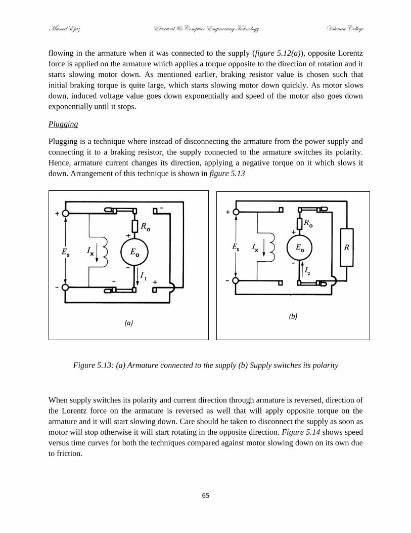
Masood Ejaz Electrical & Computer Engineering Technology Valencia College
65
flowing in the armature when it was connected to the supply (figure 5.12(a)), opposite Lorentz
force is applied on the armature which applies a torque opposite to the direction of rotation and it
starts slowing motor down. As mentioned earlier, braking resistor value is chosen such that
initial braking torque is quite large, which starts slowing motor down quickly. As motor slows
down, induced voltage value goes down exponentially and speed of the motor also goes down
exponentially until it stops.
Plugging
Plugging is a technique where instead of disconnecting the armature from the power supply and
connecting it to a braking resistor, the supply connected to the armature switches its polarity.
Hence, armature current changes its direction, applying a negative torque on it which slows it
down. Arrangement of this technique is shown in figure 5.13
Figure 5.13: (a) Armature connected to the supply (b) Supply switches its polarity
When supply switches its polarity and current direction through armature is reversed, direction of
the Lorentz force on the armature is reversed as well that will apply opposite torque on the
armature and it will start slowing down. Care should be taken to disconnect the supply as soon as
motor will stop otherwise it will start rotating in the opposite direction. Figure 5.14 shows speed
versus time curves for both the techniques compared against motor slowing down on its own due
to friction.
(a)
(b)

Masood Ejaz Electrical & Computer Engineering Technology Valencia College
66
Figure 5.14: Speed vs. Stopping Time
Example 5.5
A 120hp lap-wound motor is connected to a 240V source and rotating at 400rpm. Nominal
armature current is 400A. Dynamic braking is used to stop the motor. Calculate:
(i) Value of the braking resistance if maximum braking current is limited to 125% of its
nominal current value. Ignore the armature resistance.
The maximum braking current will flow as soon as the dynamic braking will be applied. Since
armature resistance is ignored, therefore, Eo ≈Es, and braking resistance RB = Es/IB(max) =
Es/(1.25*400) = 0.48000
(ii) Braking power if motor has decelerated to 150rpm.
Eo = Zn/60 Eo = kn, where k = Z/60, k = Eo/n = 240/400 = 0.6
Eo at 150rpm = kn = 90V
Current in the braking circuit: IB = Eo/RB = 187.5A
Therefore, braking power = EoIB = 16.875KW
Note: If armature resistance is given, you will have to consider it in the braking circuit, which
will be in series with the braking resistance.

Masood Ejaz Electrical & Computer Engineering Technology Valencia College
67
5.8 Armature Reaction
Like in generators, when substantial amount of current flows through armature in motors under
load, it produces its own magnetic field. This magnetic field interacts with the magnetic field
produced by the field electromagnets and results in a net field that not only changes the pattern
with which total flux links with the armature coils and commutator sections, thus producing
sparks at the brushes by shifting the neutral zone, but may also speed up the motor by weakening
the total flux. The problem of armature reaction in motors may be handled the same way as in
DC generators by using commutating poles.
5.9 Motor Efficiency
The efficiency of a motor is the ratio of its output mechanical power to the input electrical
power. It is generally expressed in percentage,
100%o
i
P
P (5.8)
The difference between the input and the output power is account for losses in the motor. The
smaller the losses, the higher the efficiency and vice versa.

Masood Ejaz Electrical & Computer Engineering Technology Valencia College
68
PROBLEMS
Note: Draw circuit for each problem
1. A shunt motor is connected to 230V line and running at 1000r/min. Armature current is 60A
and total armature resistance is 0.15. Armature is lap-wound with 83 slots and 6 turns per
coil. Calculate,
(i) CEMF
(ii) Power supplied to the armature
(iii) Mechanical power of the motor in KW and HP
(iv) Torque developed by the motor
(v) Flux per pole
2. A shunt motor has armature resistance of 1It is connected to 110V line and rotating at
3000 r/min. CEMF is 90V and armature is lap-wound. Calculate,
(i) Starting current
(ii) Armature current at the given induced voltage.
(iii) If dynamic braking is used and initial braking current required is 1.5 times the
armature current in (ii), determine the value of the braking resistor.
(iv) CEMF and the armature current when motor runs at 2000 r/min
3. A shunt motor is connected to line with 110V and rotating with 2000 r/min. Line current is
40A. Field resistance of motor is 100 and armature resistance is 0.2. Calculate,
(i) Armature current
(ii) CEMF
(iii) Mechanical Power
4. A compound motor has 1200 turns on the shunt winding and 25 turns on the series winding,
per pole. The shunt field has a total resistance of 115, and the armature current is 23A. If
the motor is connected to a 230V line, calculate,
(i) The mmf per pole at full load
(ii) The mmf at no-load

Masood Ejaz Electrical & Computer Engineering Technology Valencia College
69
5. A 300hp, 240V, 600 r/min motor is required to be stopped with dynamic braking technique.
If the nominal armature current is 100A, calculate,
(i) The value of braking resistor R if we want to limit the maximum braking current to
150% of its nominal value
(ii) The braking power (kW) when motor has decelerated to 200 r/min

Masood Ejaz Electrical & Computer Engineering Technology Valencia College
70
Chapter 6 - Efficiency & Heating of Machines
6.1 Types of Power Losses
There are two types of power losses in machines; mechanical and electrical.
Mechanical Losses
There are two categories of mechanical losses; frictional losses and windage losses. Frictional
losses come from any moving part in a machine including, but not limited to, brushes, bearings,
commutators, and slip rings. Windage losses come from the air friction produced by cooling fans
to remove heat from a machine.
Electrical Losses
There are three different categories of electrical losses; conductor losses, brush losses, and iron
losses.
(i) Conductor Losses: Heating loss when current flows in the field and armature
conductors.
(ii) Brush Losses: There is always some voltage drop at the brush and commutator or
brush and slip ring contact. If brush gets old or if there is improper contact, there is
more voltage drop at the contact.
(iii) Iron Losses: This loss is due to the hysteresis phenomenon in the core as well as due
to heating of the core because of eddy currents. Iron losses impose a mechanical drag
on the armature and their effect is similar to as producing mechanical friction. This is
generally measured in terms of torque calculation due to iron loss.
Figure 6.1: Losses in a DC machine

Masood Ejaz Electrical & Computer Engineering Technology Valencia College
71
6.2 Conductor Losses
If total resistance of armature conductors and field conductors is given, conductor loss can
simply be calculated using I2R, if current is known. Many times conductor type and total weight
of the conductor is given instead of total resistance of the conductor. In that situation, first, the
conductor loss in watt per kilogram is calculated using (6.1), which is multiplied by the total
conductor weight to get total conductor power loss in watt.
21000c
JP
D
(6.1)
In (6.1), J is the current density in Ampere/square millimeter (A/mm2), ρ is the resistivity of the
conductor in nano-Ohm meter (nΩ.m), and D is the density of conductor in kilogram/cubic meter
(kg/m3).
The resistivity of a specific material can be calculated using (6.2)
(1 )o T (6.2)
Where ρo is the resistivity of the material at 0oC, α is the temperature coefficient of the resistance
at 0oC, and T is the operating temperature in Celsius.
If length and area of cross section of the conductor is known, resistance of the conductor can be
calculated (if required) as shown in (6.3).
LR
A
(6.3)
The quantities ρo, α and D as required in (6.1) and (6.2) can be found in a standard table, as
shown in Table AX2 (page 918 in the textbook). Resistivity of the most commonly used
conductor, copper, is 15.88nΩ.m at 0oC, temperature coefficient at 0
oC is 4.27×10
-3/0
oC, and
density is 8890kg/m3.
6.3 Losses as a Function of Load
If there is no load connected to the machine, armature current is either zero or quite small, based
on the type of machine. Hence, armature conductor loss is either zero or very small. In this
situation, majority of the loss is comprised of frictional, windage, and iron loss. If machine has
shunt field then there is also a shunt conductor loss.

Masood Ejaz Electrical & Computer Engineering Technology Valencia College
72
As machine is loaded and armature current increases, armature conductor loss also increases.
Rest of the losses stays approximately same. The armature loss in a loaded armature contributes
to excess of heat, which may put a limit to the power supplied by the machine. Machine

Masood Ejaz Electrical & Computer Engineering Technology Valencia College
73
temperature must not exceed the maximum allowable temperature of the insulation in the
machine else windings will short and machine will not operate.
6.4 Machine Efficiency
Efficiency of a machine is measured as the ratio of its output power to input power. Generally it
is expressed in percentage.
out in loss out
in in out loss
P P P P
P P P P
(6.4)
It is important to realize that motor efficiency in the absence of iron. frictional, and windage
losses is always higher than if these losses are taken into consideration, since motor has to supply
extra current, and hence, extra power, to compensate for these losses. Although iron, frictional,
and windage losses are part of field and/or armature, for the sake of simplicity, these losses can
be lumped together and shown in parallel to the supply. This will emphasize the fact that extra
current has to be supplied by the source to compensate for these losses. A compound DC motor
with iron, frictional and windage losses can be represented by the circuit model shown in figure
6.2
Example 6.1
A DC machine is rotating at 900rpm and has armature winding that weighs 50Kg. Given
current density is 3MA/m2. Operating temperature is 90
oC. Total iron loss is 1KW. Calculate
(i) Copper loss, and (ii) Mechanical drag due to iron loss
(i) From Table AX2: Density of Cu = 88.90 Kg/m2; o = 15.88n.m; = 4.27E-3 @ 0
oC
Resistivity at 90oC: o(1 + T) = 15.88(1 + 4.27E-3*90) = 21.988n.m
Current density in A/mm2: 3E6A/1E6mm
2 = 3A/ mm
2
Copper loss/Kg: Pc = 1000J2D = (1000*3*21.98)/8890 = 22.252W/Kg
Total Copper loss: Pc*50Kg = 1.11KW
(ii) Mechanical drag due to the iron loss is calculated in terms of torque due to the iron loss, as
discussed earlier.
P = nT/9.55 T = 9.55P/n = 9.55*1000/900 = 10.611N.m

Masood Ejaz Electrical & Computer Engineering Technology Valencia College
74
Figure 6.2: DC Compound motor with iron & frictional losses
A DC shunt motor with iron and frictional losses can be represented similarly except series field
winding. Note that this model is only valid if sum of the field and the armature current is not
equal to the supply current. If supply current is equal to the sum of the field and the armature
current then do not show the iron and frictional losses in parallel, rather, they will be part of the
armature and field, and they can be represented in series with the armature and field as resistive
components to show the loss of power.
Example 6.2
A shunt motor with field resistance of 50 and armature resistance of 2 is operating at no
load. Speed of rotation is 1000rpm. The motor is lap-wound with 100 slots and 6 turns/coil.
Flux per pole is 0.1Wb. Armature current is 50A and field current is 10A. Friction and
windage losses are 1100W and iron losses are 58W. Calculate efficiency of the motor.
Copper loss in the field: Pshunt = If2Rf = 10
2*50 = 5KW
Copper loss in the armature: Pa = If2Ra = 50
2*2 = 5KW
Induced voltage: Eo = Zn/60i = (100*6*2)(1000)(0.1)/60 = 2000V
Output power: Po = EoIa = 2000*50 = 100KW
Total losses = 5KW + 5KW + 1.1KW + 58W = 11158W = 11.158KW
Efficiency: = Po/(Po + Losses) = 100/(100 + 11.158) = 0.899 = 89.9%

Masood Ejaz Electrical & Computer Engineering Technology Valencia College
75
6.5 Life Expectancy of Electric Equipment
The life expectancy of electrical equipment is limited by the temperature of its insulation. The
higher the temperature, the shorter the life. Tests have shown that the service life of a machine is
reduced by one-half every time the operating temperature rises by 10oC beyond the temperature
threshold of its insulation. Hence, a class A machine that has temperature threshold of 105oC and
normal life expectancy of eight years will have service life of four years if it is operated at
115oC. If it is operated at 125
oC, the service life will reduce to two years and so on. Extremely
low temperatures are also quite harmful as insulation can freeze and crack. There are some
special synthetic insulation materials that can operate at temperatures as high as 200oC and as
low as -60oC.
6.6 Thermal Classification of Insulators
Thermal classification of different insulators is shown in the following table (Ref: Wikipedia)
Example 6.3
A shunt motor has field resistance of 50 and armature resistance of 1. It is connected to a
200V DC source. Armature current is 10A. Friction, windage, and iron losses are 50W and
assume them to be part of the armature. Determine the efficiency of the motor.
Note: Riron represents the resistor corresponding to the loss
due to friction, windage, and iron.
Voltage drop across Riron: Eiron = Piron/Ia = 5V
Induced Voltage: Eo = Es - Ia*Ra - Eiron = 185V
Source current: Is = Ia+If = 10 + 200/50 = 14A
Input Power: Pi = Es*Is = 2800W
Output Power: Po = Eo*Ia = 1850W
Efficiency: = Po/Pi*100 = 66.071%

Masood Ejaz Electrical & Computer Engineering Technology Valencia College
76
Table 6.1: Classes of Insulation Systems
6.7 Speed and Size of a Machine
Although the nominal power rating of a machine depends upon the maximum allowable
temperature rise but its size depends upon the power and speed of rotation. This, in turns, results
in the size of motor depending upon torque that it develops. Thus, a 100KW motor running at
2000 rpm is approximately the same size as 10KW motor running at 200 rpm as they develop the
same torque. This results in low-speed motors to be quite costly as compared to high-sped
motors to produce the same power. Hence, if load requires low-speed, generally it is preferred to
use a high-speed motor coupled with a gear to turn the load at low speeds rather than connecting
load directly to a low-speed motor.
Masood Ejaz Electrical & Computer Engineering Technology Valencia College
77
PROBLEMS
1. A DC shunt motor with field resistance of 110 and total armature resistance of 0.6 has
17A armature current. It is connected to 110V, 20A line. CEMF is 100V, calculate,
(i) Total copper losses (I2R losses)
(ii) Total mechanical + iron losses
(iii) Efficiency
2. A DC compound motor has shunt field resistance of 500 and series field resistance of 2.
Shunt field current is 0.44A. Armature is lap wound with 200 conductors running at 600rpm.
Flux per pole is 0.1Wb. Armature winding resistance is 0.1 and it is dissipating 10W. Other
losses amount to 35W. Calculate the efficiency of the motor.

Masood Ejaz Electrical & Computer Engineering Technology Valencia College
78
Chapter 7 – Active, Reactive, and Apparent Power
7.1 Different Types of Power
In a power system, there are different types of power with different units. These power types
include:
(i) Instantaneous Power
(ii) Active Power
(iii)Reactive Power
(iv) Complex Power
(v) Apparent Power
For any power system and any load, values for all power types can be calculated although many
times it is either not required or already known. Description of each power type is given in the
following sections.
7.2 Instantaneous Power
When voltage and current are function of time, their product gives instantaneous power, i.e.
power at any instant of time. Let v is the voltage applied across some device and current i flows
in it, as shown in figure 7.1
Figure 7.1: Voltage ‘v’ applied to a device requiring current ‘i’
If both voltage and currents are sinusoidal in nature, they can be represented by the following
generic time-domain expressions:
( ) ( ) (Volt)
( ) ( ) (Ampere)
p
p
v t V cos t
i t I cos t
(7.1)
where Vp and Ip are the peak values of voltage and current waveforms, and and are their
corresponding phase angles, respectively.
The instantaneous power supplied to the device can be given by:

Masood Ejaz Electrical & Computer Engineering Technology Valencia College
79
( ) ( ) ( ) cos( )cos( ) (Watt)p t v t i t VpIp t t (7.2)
Unit of instantaneous power is Watt.
Analysis of electrical networks with sinusoidal signals is generally done in complex frequency
phasor domain instead of time domain as it converts integro-differential circuit equations into
simple algebraic equations with complex numbers. For the voltage and current given in (7.1), the
equivalent phasor quantities will be given by:
( )
( )
p
p
j V
j I
V
I (7.3)
Make sure that the signals are still time-domain signals but for the sake of analysis in the
complex frequency domain, they are written as complex numbers in polar form where magnitude
of the signal is the peak value and angle is the phase of the signal. Equivalently, the complex
frequency notations can also be given in Cartesian form as complex numbers. Once analysis of
the circuit is done in the complex frequency domain, the result is converted back in time domain
by writing it in the form Acos(t+B), where A is the peak value and B is the phase of the
resultant quantity.
The device as shown in figure 7.1 is associated with an impedance which can be calculated by
dividing phasor quantity of voltage by the phasor quantity of current given in (7.3),
( )( )
( )
p p
p p
V Vjj
j I I
VZ
I (7.4)
where the magnitude of the impedance is Vp/Ip and its phase is
7.3 Active Power
Active power has many other names; real power, average power, DC power etc. This is the
average power consumed in a device or supplied by a source over one cycle. To calculate
average or active power, calculate the average of p(t) given in (7.2) over one time period, as
shown below.

Masood Ejaz Electrical & Computer Engineering Technology Valencia College
80
0 0
2
0
2
0
1 1( ) cos( )cos( )
1cos( )cos( )
2
cos(2 ) cos( )
2 2
cos( ) cos( ) cos( )2 2 2
T T
t t
t
t
rms rms
P p t dt VpIp t t dtT T
VpIp t t d t
VpIp td t
VpIp Vp IpV I
(7.5)
Hence, active power is given by cos( )rms rmsV I or cosrms rmsV I Z . Unit of active power is
Watt. This is the power that produces some tangible quantity. For example, conversion of
electrical energy into light energy, mechanical energy, heat energy etc. Also, this is the power
that is measured by kilowatt-hour meters and consumers are charged for.
Active power is the power that is dissipated in the resistive part of the network only; hence this is
not the power associated with inductors and capacitors, i.e. the reactive part of the electric
network. Hence, if there are multiple resistors in the network, total active power supplied is the
sum of power dissipated in each resistor,
2 2 2 22 2 2 1 2 3
1 1 2 2
1 2 3
cos nrms rms n n
n
V V V VP V I I R I R I R
R R R R Z L L (7.6)
where In is the rms value of the current and Vn is the rms value of the voltage across n-th resistor.
Be very careful if you are using V2/R formula to calculate active power as the value of rms
voltage used is the voltage across resistor only, not the whole load, if it is comprised of resistor
and capacitor and/or inductor.
If a 10V (peak) sinusoidal source is applied across a 1 resistor, it will produce a sinusoidal
current with peak value of 1A. When the voltage and current waveforms, which are in phase, are
multiplied by each other, instantaneous power waveform is generated. All three waveforms are
shown in figure 7.1. Observe that power waveform is only unidirectional, i.e. above the zeroaxis.
Hence, an average value of this power exists, which is given by (7.5) or (7.6). This is the
active power supplied by the source or dissipated in the load resistor.

Masood Ejaz Electrical & Computer Engineering Technology Valencia College
81
Figure 7.1: Voltage Waveform (blue), Current Waveform (red), and Power Waveform (green) in
a 1 Resistor
7.4 Reactive Power
As it was discussed in the previous section, average or active power supplied by a source is
consumed in the resistive part of the network. This is the power that is measured through
kilowatt hour meters and everyone pay bill to consume it. In the study of generators and motors
it was discussed that current is required to setup magnetic field in the machine through coils
(inductors). The power that is used to setup this magnetic field is not active power as it is not
delivered to the resistive part of the circuit, rather it is reactive power. In general, reactive power
is the power related to the reactive part (inductor and capacitor) of the circuit. This power cannot
be measured through kilo-watt hour meters but there are special meters, called VAR-meters to
measure it.
The reactive power supplied or consumed in the reactive components can be given by,
sin( )rms rmsQ V I (7.7)
Unit of measuring reactive power is Volt-Ampere Reactive (VAR). Observe that current lags
voltage by 90o
in an inductor and leads by 90o in a capacitor. Hence, reactive power absorbed by
inductor is positive, since is positive, and it is negative in capacitor since is negative.
Therefore, on average, inductor absorbs reactive power and capacitor supplies reactive power. In
other words, in phasor (complex frequency) domain, current goes in an inductor and comes out
of a capacitor.
Magnitude of reactive power in an inductor or capacitor can also be measured by applying
Ohm’s law on the basic power expression as follows:

Masood Ejaz Electrical & Computer Engineering Technology Valencia College
82
22| | rms
rms
VQ I X
X
(7.8)
Make sure that reactive power measured using (7.8) should be appended by a negative sign if it
is a capacitor.
Voltage, current, and power waveforms through a capacitor and an inductor are shown in figure
7.2(a) and (b) respectively. Observe that current is leading the voltage by 90o in capacitor
(current is maximum when voltage is zero) and lagging 90o in inductor (current is minimum
when voltage is zero). In any case, power waveform is a pure sinusoid. Hence, average power is
zero. Therefore, as discussed earlier, there is no average or active power associated with reactive
components.
Figure 7.2: Voltage (Blue), Current (Red), and Power (Green) Waveforms across Capacitor (a)
and Inductor (b)
7.5 Current Components
Let v(t) = Vmcos(t) is applied across an impedance and current i(t) = Imcos(t + ) flows
through it. In phasor domain, the time-domain quantities can be written as Vm∠0 and
Im∠±Observe that current in phasor domain has two components; Imcos(andImsin, as
shown in figure 7.3
Figure 7.3: Components of current
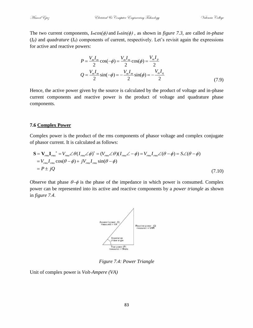
Masood Ejaz Electrical & Computer Engineering Technology Valencia College
83
The two current components, Imcos(andImsin , as shown in figure 7.3, are called in-phase
(Ip) and quadrature (Iq) components of current, respectively. Let’s revisit again the expressions
for active and reactive powers:
cos( ) cos( )2 2 2
sin( ) sin( )2 2 2
m pm m m m
m qm m m m
V IV I V IP
V IV I V IQ
(7.9)
Hence, the active power given by the source is calculated by the product of voltage and in-phase
current components and reactive power is the product of voltage and quadrature phase
components.
7.6 Complex Power
Complex power is the product of the rms components of phasor voltage and complex conjugate
of phasor current. It is calculated as follows:
( ) ( )( ) ( ) ( )
cos( ) sin( )
rms rms rms rms rms rms rms rms
rms rms rms rms
V I V I V I S
V I jV I
P jQ
S V I
(7.10)
Observe that phase is the phase of the impedance in which power is consumed. Complex
power can be represented into its active and reactive components by a power triangle as shown
in figure 7.4.
Figure 7.4: Power Triangle
Unit of complex power is Volt-Ampere (VA)

Masood Ejaz Electrical & Computer Engineering Technology Valencia College
84
7.7 Apparent Power
Apparent power is the magnitude of complex power. It is measured in Volt-Ampere (VA). As
given in (7.10), apparent power is given by:
rms rmsS V I (7.11)
Observe that apparent power appears in the expressions of active and reactive power as given by
(7.5) and (7.7), hence, another way to calculate it is as follows:
cos( ) sin( )
P QS
(7.12)
Example 7.1
A Wattmeter and a VARmeter are connected to an AC line with 155.56V peak value. An AC
motor is connected to the line for which the wattmeter is recording 2000W and the VARmeter
is recording 1000VAR. Calculate:
(i) In-phase and Quadrature components of the motor current:
>>Espeak = 155.56; EsRMS = Espeak/ = 110V
In-phase component: Ip = P/EsRMS = 18.182A
Quadrature component: Iq = Q/EsRMS = 9.0911A
(ii) Total current: I = = 20.328A
(iii) Apparent Power: |S| = ERMS*I = 2236.1VA
(iv) Phase angle between voltage and current or impedance angle of the motor:
∠V-∠I = ∠Z tan-1
(Q/P) = 26.565o

Masood Ejaz Electrical & Computer Engineering Technology Valencia College
85
7.8 Power Factor
Power factor is an extremely important quantity in power systems. It is the quantity that
describes the type of load and the amount of bill that we pay to the electrical company. Power
factor is the cosine of the phase of load impedance,
cos( )PF (7.13)
Hence, power factor is unity if the load is pure resistive (voltage and current are in phase) and
zero if the load is pure reactive (voltage and current are perpendicular to each other). For real
loads, power factor is between zero and one. Remember that the active power is measured by
Scos(-) or (S)(PF). Hence, active power is maximum when power factor is unity or load is
pure resistive and it is zero if load is pure reactive and power factor is zero. Hence, when power
factor is unity, power company gets the full amount of power supplied to the consumer and if
power factor is zero, consumer pays nothing despite receiving reactive power (i.e. load current)
from the power company. For real loads, power companies adjust the bill based on power factor
correction to receive the fair amount of compensation for the energy supplied by them.
Power factor is generally represented in percentage (0-100%). Also, based on the load type
(capacitive or inductive), it is represented as leading or lagging power factor. If current leads
voltage for the load, i.e. if load is capacitive, power factor is leading else it is lagging.
Example 7.2
A motor draws 10A from 110V (rms), 60Hz line with the power factor of 80% lagging.
Determine the active power absorbed by the motor and the reactive power supplied by the line.
(i) Active power absorbed by the motor:
P = Es*I*PF = 880 W
(i) Reactive power supplied by the line which will be absorbed
by the motor:
Q = Es*I*sin(cos-1(PF))= 660VAR
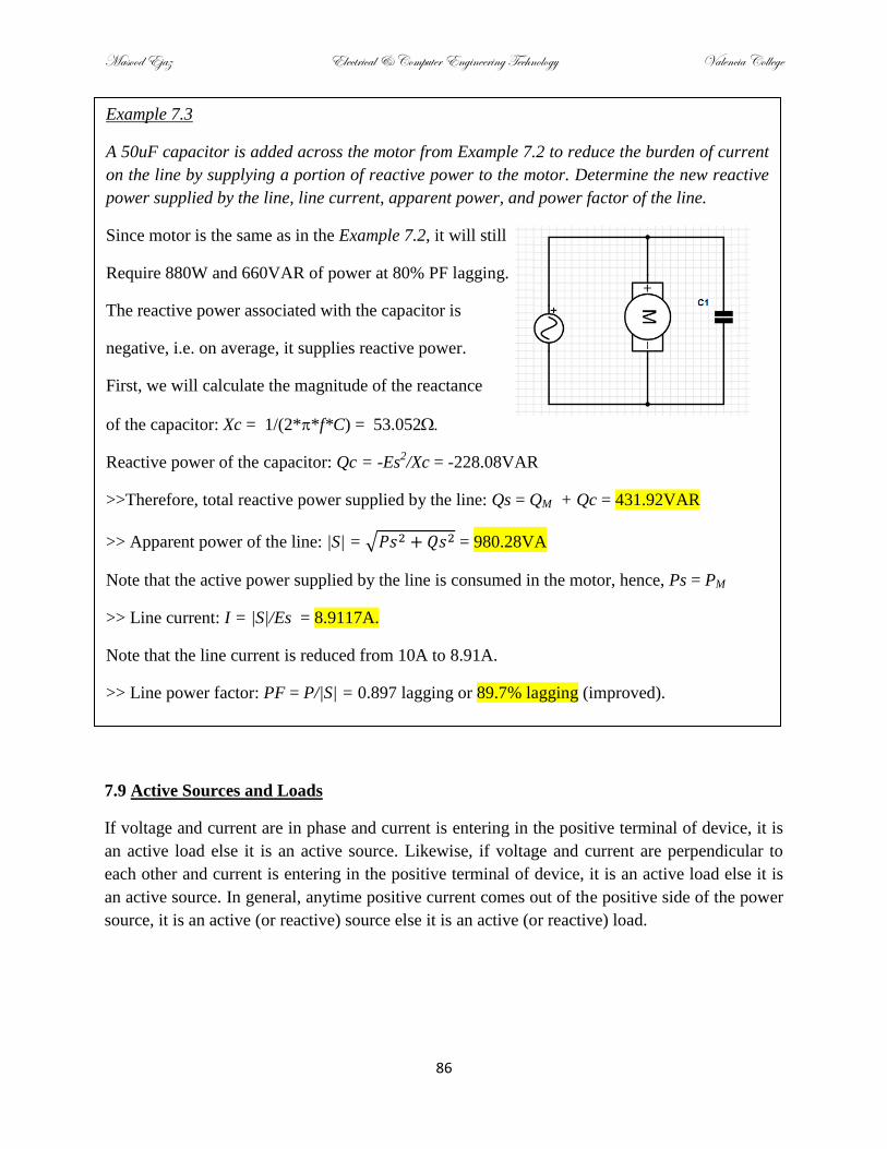
Masood Ejaz Electrical & Computer Engineering Technology Valencia College
86
7.9 Active Sources and Loads
If voltage and current are in phase and current is entering in the positive terminal of device, it is
an active load else it is an active source. Likewise, if voltage and current are perpendicular to
each other and current is entering in the positive terminal of device, it is an active load else it is
an active source. In general, anytime positive current comes out of the positive side of the power
source, it is an active (or reactive) source else it is an active (or reactive) load.
Example 7.3
A 50uF capacitor is added across the motor from Example 7.2 to reduce the burden of current
on the line by supplying a portion of reactive power to the motor. Determine the new reactive
power supplied by the line, line current, apparent power, and power factor of the line.
Since motor is the same as in the Example 7.2, it will still
Require 880W and 660VAR of power at 80% PF lagging.
The reactive power associated with the capacitor is
negative, i.e. on average, it supplies reactive power.
First, we will calculate the magnitude of the reactance
of the capacitor: Xc = 1/(2**f*C) = 53.052
Reactive power of the capacitor: Qc = -Es2/Xc = -228.08VAR
>>Therefore, total reactive power supplied by the line: Qs = QM + Qc = 431.92VAR
>> Apparent power of the line: |S| = = 980.28VA
Note that the active power supplied by the line is consumed in the motor, hence, Ps = PM
>> Line current: I = |S|/Es = 8.9117A.
Note that the line current is reduced from 10A to 8.91A.
>> Line power factor: PF = P/|S| = 0.897 lagging or 89.7% lagging (improved).
Masood Ejaz Electrical & Computer Engineering Technology Valencia College
87
7.10 System Comprising of Several Loads
A power system is comprised of several loads; some active and some reactive. The total active
power supplied by the power system is the sum of active power consumed in all of the active
loads. Likewise, the total reactive power supplied by the system is the net reactive power
consumed by all of the reactive components. Keep in mind that reactive power to inductive loads
is considered to be positive, i.e. positive current flows in the positive terminal of the inductive
component, whereas, reactive power to the capacitive loads is negative, i.e. positive current
comes out of the positive terminal of the capacitive components. Hence, net reactive power
supplied by the system is the difference between the power supplied to the inductive part and
received from the capacitive part.
Example 7.4
A power system with Es = 220V(rms) is furnishing the following loads:
Resistive: 8KW, 14KW, and 2KW
Inductive: 7KVAR, 8KVAR, and 5KVAR
Capacitive: 16KVAR and 9KVAR
Calculate:
(i) Total active power absorbed by the load: P = 8+14+2 = 24KW
(ii) Total reactive power supplied by the line: Q = QL + Qc = (7 + 8 + 5) – (16 + 9) = -5KVAR
Therefore, line is receiving 5KVAR of reactive power from the load.
(iii) Apparent power of the system: |S| = = 24.515KVA
(iv)Line current: I = |S|/Es| = 111.43A
(v) Power factor of the system: PF = P/|S| = 0.978 leading or 97.8% leading.
Note that since the total reactive power is negative, source sees load as a capacitive load for
which power factor is leading, since current leads voltage in capacitive loads.
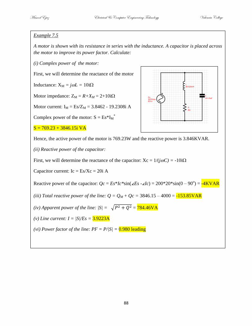
Masood Ejaz Electrical & Computer Engineering Technology Valencia College
88
Example 7.5
A motor is shown with its resistance in series with the inductance. A capacitor is placed across
the motor to improve its power factor. Calculate:
(i) Complex power of the motor:
First, we will determine the reactance of the motor
Inductance: XM = jL = 10i
Motor impedance: ZM = R+XM = 2+10i
Motor current: IM = Es/ZM = 3.8462 - 19.2308i A
Complex power of the motor: S = Es*IM*
S = 769.23 + 3846.15i VA
Hence, the active power of the motor is 769.23W and the reactive power is 3.846KVAR.
(ii) Reactive power of the capacitor:
First, we will determine the reactance of the capacitor: Xc = 1/(jC) = -10i
Capacitor current: Ic = Es/Xc = 20i A
Reactive power of the capacitor: Qc = Es*Ic*sin(∠Es -∠Ic) = 200*20*sin(0 – 90o) = -4KVAR
(iii) Total reactive power of the line: Q = QM + Qc = 3846.15 – 4000 = -153.85VAR
(iv) Apparent power of the line: |S| = = 784.46VA
(v) Line current: I = |S|/Es = 3.9223A
(vi) Power factor of the line: PF = P/|S| = 0.980 leading

Masood Ejaz Electrical & Computer Engineering Technology Valencia College
89
PROBLEMS
Note: RMS values of all voltages and currents are given. If in any problem, peak values are
given then convert them into RMS first before you calculate active, reactive, apparent, and
complex powers.
1. A motor draws 20A from 110V, 60Hz line with power factor of 77% lagging, calculate,
(i) Active power absorbed by the motor
(ii) Reactive power supplied by the line
(iii) In-phase current component
(iv) Quadrature current component
(v) Resistance of the motor
(vi) Reactance of the motor
(vii) Impedance of the motor
2. If a 1000 uF capacitor is placed at the terminals of the motor in problem # 1 to reduce the
amount of current, what will be the new value of line current and new PF of the motor?
Assume that motor still requires same active and reactive power as being calculated in the
last problem.
3.
Note: average power is same as active power

Masood Ejaz Electrical & Computer Engineering Technology Valencia College
90
Chapter 8 – Three-Phase Circuits
Electrical Power is generated, transmitted, and distributed in the form of three-phase power.
There are certain advantages of a three-phase power system over a single-phase system:
Three-phase systems are not much complicated as compared to a single-phase system.
They are cheaper and more efficient
Three-phase transmission lines can deliver more power for a given weight and cost
Voltage regulation for three-phase transmission lines is better
In U.S.A, homes usually have a single-phase system; it is one of the phases of the three-phase
system stepped down to 110V(rms)/120V(rms) with a center-tapped step-down transformer.
Homes in many other countries get all three phases coming to them with different loads
distributed on different phases.
Note that some of the appliances in our homes require 220V(rms)/240V(rms) instead of
110V(rms)/120V(rms). This is done by connecting the two 180o out-of-phase terminals of the
center-tapped transformer to create a 220V(rms)/240V(rms) voltage socket, as shown in the
following figure. Observe that this circuit doesn’t have a neutral wire, rather two same 180o out-
of-phase hot (phase) wires between which the load will be connected. It is still a single-phase
system.
Figure 8.1: Center-tapped step-down transformer that provides power to homes
A three-phase system provides voltage between three lines that have same peak and root-mean-
square (rms) values but they are 120o out-of-phase with each other. Hence, the instantaneous
value of the voltage for each line is different. A common depiction of a three-phase system and
its voltage waveforms is shown in figure 8.2. In the figure, VA, VB and VC are three line-to-neutral
voltages, also called phase voltages, and VAB is line-to-line voltage, also referred to as simply
line voltage.

Masood Ejaz Electrical & Computer Engineering Technology Valencia College
91
Figure 8.2: (a) Representation of a Three-phase System (b)Phase Voltages
8.1 Single-Phase Generator
To appreciate the constructional advantage and characteristics of a three-phase system, it is
important to compare it against single-phase and two-phase generator systems. The basic AC
generator that we discussed in chapters 2 and 4 is a single phase generator. However,
commercial AC generators generally have rotating magnetic field and static conductors in which
voltage is induced. This arrangement of rotating magnet (rotor) and static voltage inducing
conductors (stator) yield alternating current generators or synchronous generators. Detailed
characteristics of synchronous generators will be studied in a later chapter. In this chapter, we
will use the generator concepts that we have developed so far, simply to determine the output of
synchronous generators.
Observe the arrangement of a single-phase synchronous AC generator with a permanent magnet
as rotor and conductor coils on stator, as shown in figure 8.3
Figure 8.3: Construction of a simple single-phase AC generator
(a)
(b)
(a)
(b)

Masood Ejaz Electrical & Computer Engineering Technology Valencia College
92
Note that we can use the equation l.(v x B) to calculate the value of the induced voltage in the
coil. However, care should be taken about the direction of the velocity. In the expression l.(v x
B), v is the velocity of the armature or conductor coils. In the AC generator under discussion,
conductors are stationary but magnet is moving. Hence, the velocity of conductors becomes
relative velocity with respect to the magnet. Assume that you are sitting on the magnet which is
rotating with a velocity of v in the counter-clockwise direction. When you look at the conductors
from the magnet, it will appear to move in the opposite, i.e. clockwise direction. Hence, relative
velocity of conductors will always be opposite to the direction of the rotation of magnet and that
direction will be used in the expression to calculate induced voltage and its direction.
In figure 8.3(a), the relative velocity of side a of the conductor is –j, the direction of the
magnetic flux is –k, hence v x B will yield a direction of i. Therefore, polarity of the induced
voltage in the side a of the conductor will be positive with respect to the side 1, and if shorted,
current is going to come out of the side a and will go into the side 1. When the magnet will rotate
to 90o, as shown in figure 8.3(b), flux will not cut the conductors and hence, the induced voltage
will be zero. The output waveform for one cycle is usually near sinusoid but for the sake of
simplicity we will assume the output to be a pure sinusoidal waveform, as shown in figure 8.4
Figure 8.4: Output of a single-phase AC generator
If a resistor is connected to the terminals of the generator, the average or real power supplied will
be,
P = VrmsIrms =
Watt (8.1)
8.2 Two-Phase Generator
The only difference between a single-phase and a two-phase generator is that there are two
separate sets of windings on the stator, as shown in figure 8.5. These windings are isolated from
each other and two separate sets of voltages are induced in them, which have a phase difference
of 90o between them.
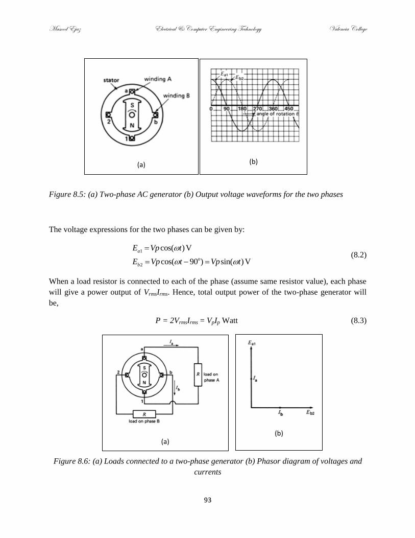
Masood Ejaz Electrical & Computer Engineering Technology Valencia College
93
Figure 8.5: (a) Two-phase AC generator (b) Output voltage waveforms for the two phases
The voltage expressions for the two phases can be given by:
1
2
cos( )V
cos( 90 ) sin( )V
a
b
E Vp t
E Vp t Vp t
o (8.2)
When a load resistor is connected to each of the phase (assume same resistor value), each phase
will give a power output of VrmsIrms. Hence, total output power of the two-phase generator will
be,
P = 2VrmsIrms = VpIp Watt (8.3)
Figure 8.6: (a) Loads connected to a two-phase generator (b) Phasor diagram of voltages and
currents
(a)
(b)
(a)
(b)
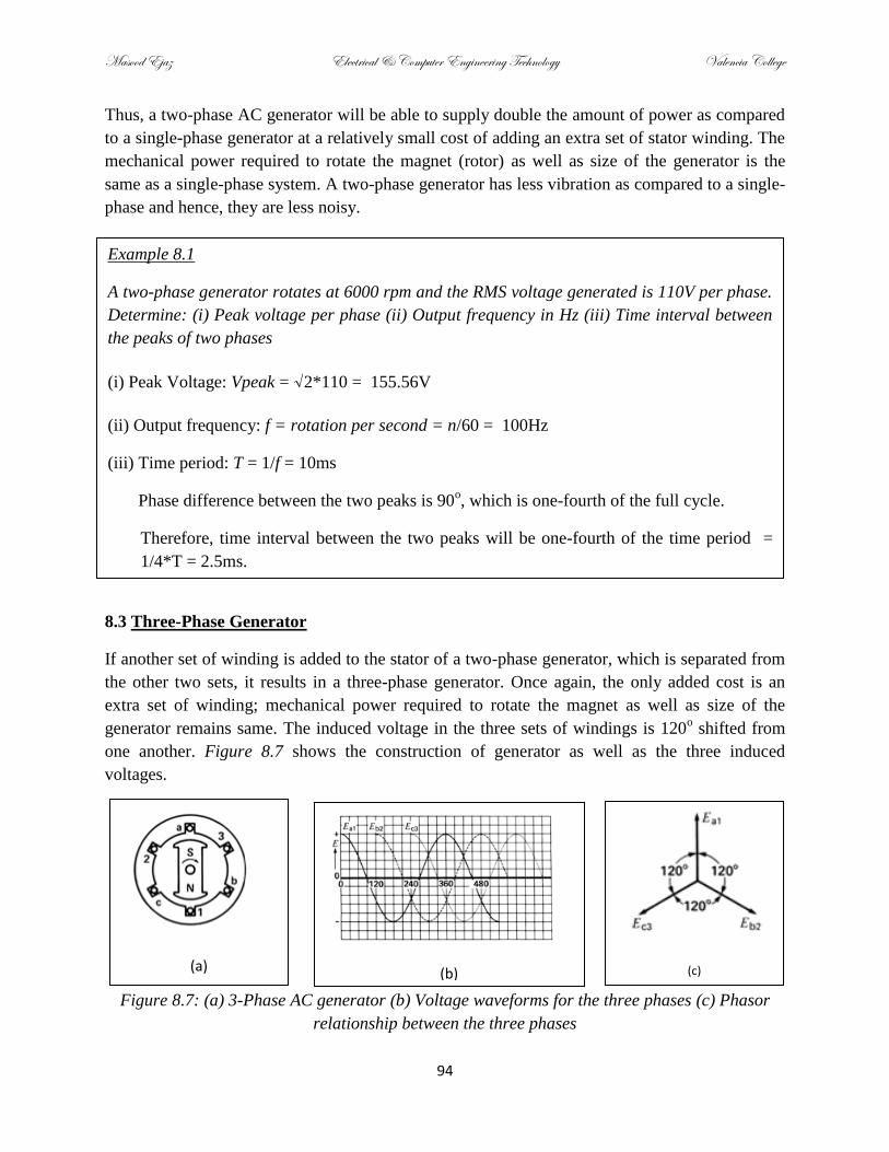
Masood Ejaz Electrical & Computer Engineering Technology Valencia College
94
Thus, a two-phase AC generator will be able to supply double the amount of power as compared
to a single-phase generator at a relatively small cost of adding an extra set of stator winding. The
mechanical power required to rotate the magnet (rotor) as well as size of the generator is the
same as a single-phase system. A two-phase generator has less vibration as compared to a single-
phase and hence, they are less noisy.
8.3 Three-Phase Generator
If another set of winding is added to the stator of a two-phase generator, which is separated from
the other two sets, it results in a three-phase generator. Once again, the only added cost is an
extra set of winding; mechanical power required to rotate the magnet as well as size of the
generator remains same. The induced voltage in the three sets of windings is 120o shifted from
one another. Figure 8.7 shows the construction of generator as well as the three induced
voltages.
Figure 8.7: (a) 3-Phase AC generator (b) Voltage waveforms for the three phases (c) Phasor
relationship between the three phases
(a)
(b)
(c)
Example 8.1
A two-phase generator rotates at 6000 rpm and the RMS voltage generated is 110V per phase.
Determine: (i) Peak voltage per phase (ii) Output frequency in Hz (iii) Time interval between
the peaks of two phases
(i) Peak Voltage: Vpeak = √2*110 = 155.56V
(ii) Output frequency: f = rotation per second = n/60 = 100Hz
(iii) Time period: T = 1/f = 10ms
Phase difference between the two peaks is 90o, which is one-fourth of the full cycle.
Therefore, time interval between the two peaks will be one-fourth of the time period =
1/4*T = 2.5ms.

Masood Ejaz Electrical & Computer Engineering Technology Valencia College
95
The three phase voltages can be given by the following expressions:
1
2
3
cos( )V
cos( 120 )
cos( 240 ) cos( 120 )
a
b
c
E Vp t
E Vp t
E Vp t Vp t
o
o o
(8.4)
Total average power for the three-phase generator is the sum of the average power of each phase,
which is VrmsIrms. Therefore, total average power is given by,
P = 3VrmsIrms =
VpIp Watt (8.5)
Hence, total average power output is 1.5 times the output of a single-phase generator, which is a
great gain at the expense of a little cost of additional conductors on the stator.
8.4 Circuit Representation of a Three-Phase System
There are three circuit representations of a three-phase generator; six-wire circuit, four-wire
circuit (most commonly used), and three-wire circuit.
Six-wire System: This is the original representation of a three-phase generator shown in figure
8.7(a). The equivalent circuit is shown in figure 8.8
Figure 8.8: Six-Wire Three-Phase System
To reduce the number of conductors, a single wire is used as return, which is called neutral. This
results in a four-wire system, as shown in figure 8.9

Masood Ejaz Electrical & Computer Engineering Technology Valencia College
96
Figure 8.9: Four-Wire three-Phase System
For a balanced system, as shown in figure 8.9, sum of the three phase currents will be equal to
zero, as can be shown by (8.6)
120 240
120 240
(1 0.5 0.866 0.5 0.866) 0
an bn cnn a b c
o o
p p p
o o
p p p
p
R R R
V V V
R R R
I I I
I j j
V V VI I I I
(8.6)
Since there is no current in the neutral wire for a balanced three-phase system, it is possible to
remove the neutral and represent a balanced three-phase system by a three-wire circuit, as shown
in figure 8.10
Figure 8.10: Three-Wire Three-Phase Balanced System
The three-phase system and the load shown in figures 8.9 and 8.10 are said to be organized in
wye configuration. The three-phase system is always in wye, whereas load can be connected
either in wye, between line and neutral, or delta, between two lines (line-to-line).

Masood Ejaz Electrical & Computer Engineering Technology Valencia College
97
8.5 Relationship Between Line-to-Neutral and Line-to-Line Voltages
Line-to-neutral voltage, also called phase voltage is between each phase and neutral. A load
connected in wye always experience phase voltage across it (if there is no line impedance). Line-
to-line voltage, also called simply line voltage is between two phases. Hence, line voltages in a
three-phase system are Eab, Ebc, and Eca. Let’s look at the value of each line voltage.
0 120 (1 (cos( 120 ) sin( 120 )))
1 0.5 0.866 1.5 0.866 1.732 30 3 30
ab an bn p p p
p p p p
E E E j
E j E j E E
E E Eo o o o
o o (8.7)
Likewise, the value of Ebc and Eca can be given by,
3 90 & 3 150bc p ca pE E E Eo o (8.8)
Hence, the magnitude of line voltages is times the magnitude of phase voltages:
3LL LNE E (8.9)
Also, line voltages are 120o apart similar to phase voltages. A phasor diagram with phase and
line voltages is shown in figure 8.11
Figure 8.11: Phasor diagram of phase and line voltages
Example 8.2
A 3-phase generator generates a line voltage of 300V(peak). There is a balanced load of
100 connected to the system (refer to figure 8.9). Calculate (i) Voltage across each resistor
(ii) Current in each resistor (iii) Total output power of the generator.
(i) Since load is connected in wye, voltage across each resistor is the line-to-neutral voltage;
ELN(peak) = ELL(peak)/sqrt(3) = 173.21V
(ii) IR = ELN(peak) /R = 1.7321A
(iii) P= 3*ELN(peak) *I/2 = 450W
>>

Masood Ejaz Electrical & Computer Engineering Technology Valencia College
98
8.6 Delta Connection
If a three-phase load is connected between line-to-line instead of line-to-neutral, it makes a delta
connection, as shown in figure 8.12
Figure 8.12: A Three-Phase load connected in delta
Hence, line-to-line voltage appears across each impedance of a delta-connected load. Let’s look
at the relationship between line currents (IA, IB, and IC) and load currents (IAB, IBC, and ICA):
3
1.5 0.866 ( 1.5 0.866)
3 3 33
p pAB CAA AB CA
p LLLoad
E Ej j
Z Z Z Z
E EI
Z Z
E EI I I
(8.10)
Likewise, IB and IC are given by,
3 120 & 3 120B Load C LoadI I I Io o
(8.11)
Hence, the magnitude of line currents is equal to times the magnitude of load currents when
the load is connected in delta configuration.
Example 8.3
A 3-phase system has a phase voltage of 220V(rms). There is a balanced load connected in
delta to the system (refer to figure 8.12). Each line current is 10A. Calculate (i) load current
(ii) magnitude of each impedance.
(i) ILOAD = ILine/sqrt(3) = 5.7735A
(ii) Since load is connected in delta, voltage across each impedance is the line voltage;
ELL(rms) = sqrt(3)*ELN(rms) = 381.05V
Magnitude of each impedance: Z = ELL/Iload = 66
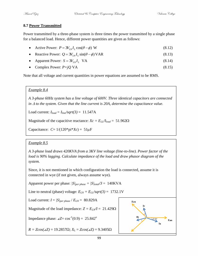
Masood Ejaz Electrical & Computer Engineering Technology Valencia College
99
8.7 Power Transmitted
Power transmitted by a three-phase system is three times the power transmitted by a single phase
for a balanced load. Hence, different power quantities are given as follows:
Active Power: 3 cos( )LN LP V I W (8.12)
Reactive Power: 3 sin( )LN LQ V I VAR (8.13)
Apparent Power: 3 LN LS V I VA (8.14)
Complex Power: P+jQ VA (8.15)
Note that all voltage and current quantities in power equations are assumed to be RMS.
Example 8.4
A 3-phase 60Hz system has a line voltage of 600V. Three identical capacitors are connected
in to the system. Given that the line current is 20A, determine the capacitance value.
Load current: Iload = Iline/sqrt(3) = 11.547A
Magnitude of the capacitive reactance: Xc = ELL/Iload = 51.962
Capacitance: C= 1/(120*pi*Xc) = 51F
Example 8.5
A 3-phase load draws 420KVA from a 3KV line voltage (line-to-line). Power factor of the
load is 90% lagging. Calculate impedance of the load and draw phasor diagram of the
system.
Since, it is not mentioned in which configuration the load is connected, assume it is
connected in wye (if not given, always assume wye).
Apparent power per phase: |S|per phase = |S|total/3 = 140KVA
Line to neutral (phase) voltage: ELN = ELL/sqrt(3) = 1732.1V
Load current: I = |S|per phase / ELN = 80.829A
Magnitude of the load impedance: Z = ELN/I = 21.429
Impedance phase: ∠Z= cos-1
(0.9) = 25.842o
R = Zcos(∠Z) = 19.2857; XL = Zcos(∠Z) = 9.3405
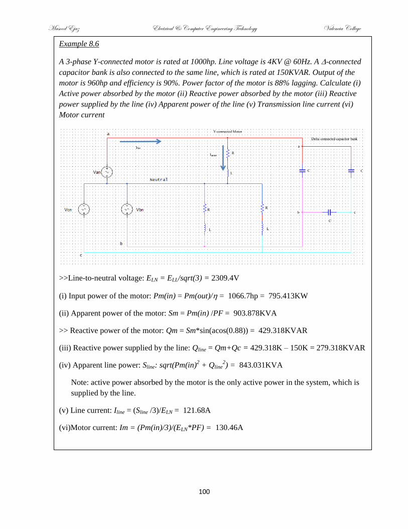
Masood Ejaz Electrical & Computer Engineering Technology Valencia College
100
Example 8.6
A 3-phase Y-connected motor is rated at 1000hp. Line voltage is 4KV @ 60Hz. A -connected
capacitor bank is also connected to the same line, which is rated at 150KVAR. Output of the
motor is 960hp and efficiency is 90%. Power factor of the motor is 88% lagging. Calculate (i)
Active power absorbed by the motor (ii) Reactive power absorbed by the motor (iii) Reactive
power supplied by the line (iv) Apparent power of the line (v) Transmission line current (vi)
Motor current
>>Line-to-neutral voltage: ELN = ELL/sqrt(3) = 2309.4V
(i) Input power of the motor: Pm(in) = Pm(out)/ = 1066.7hp = 795.413KW
(ii) Apparent power of the motor: Sm = Pm(in) /PF = 903.878KVA
>> Reactive power of the motor: Qm = Sm*sin(acos(0.88)) = 429.318KVAR
(iii) Reactive power supplied by the line: Qline = Qm+Qc = 429.318K – 150K = 279.318KVAR
(iv) Apparent line power: Sline: sqrt(Pm(in)2 + Qline
2) = 843.031KVA
Note: active power absorbed by the motor is the only active power in the system, which is
supplied by the line.
(v) Line current: Iline = (Sline /3)/ELN = 121.68A
(vi)Motor current: Im = (Pm(in)/3)/(ELN*PF) = 130.46A

Masood Ejaz Electrical & Computer Engineering Technology Valencia College
101
Example 8.7
A 3-phase balanced load comprised of three impedances Z = 100∠30o is connected to 60Hz,
220V(rms)(phase voltage) system. Synchronous (line) reactance and resistance are 10 and
2 per phase, respectively. Determine total active and reactive power delivered to the load.
Since the system is balanced, you can solve for a single phase and then extend your results for
all the other phases. Single-phase equivalent circuit is shown in the following circuit diagram.
>> Vphase = 220V; Rs = 2; Xs = j10;
>> Z = 100*cos(30) + i*100*sin(30) = 86.603 + j50.000
Line current: >> I = Vphase/(Z + Rs + Xs) = 1.7023 - j1.1528A = 2.0559∠-34.105oA
Active load power per phase: P(per phase) = |I|2*Rload = 366.06W
Reactive load power per phase: Q(per phase) = |I|2*|Xload| = 211.35VAR
Total load active power = 3*P(per phase) = 1098.2W
Total load reactive power = 3* Q(per phase) = 634.04VAR

Masood Ejaz Electrical & Computer Engineering Technology Valencia College
102
PROBLEMS
Note: If a 3-phase connection is not mentioned, always assume wye. If peak value is not
mentioned then assume that RMS value of voltages and currents are given.
1. A large 3-phase, 4000V (line-to-line), 60Hz motor draws a current of 385A (per phase) and a
total active power of 2344KW when operating at full load. Total copper losses are 15KW,
iron losses are 23.4KW, and windage and friction losses are 12KW. Motor is rotating at 800
rpm. Calculate the following:
(i) The power factor at full-load
(ii) Output mechanical power
(iii) Output torque
(iv) Efficiency
2. A 3-phase generator possesses a synchronous reactance of 6(line reactance between the
source and the load) and the excitation voltage Eo = 3KV (source) per phase. Calculate the
line-to-neutral voltage ELoad for a balanced resistive load of 8. Also, draw a phasor diagram
between three-phase source and load voltages.
3. A 3-phase generator connected in wye has the following characteristics: Eo = 2440V, line
reactance Xs = 144, line resistance Rs = 17. Assume that there is 175 resistance
connected as a load per phase. Calculate:
(i) The line current
(ii) Line-to-neutral and line-to-line voltage across the load
(iii) Phasor diagram between source and load voltages
4. A 3-phase generator delivers power to a 2400 KVA (total), 16KV (line-to-neutral) load
having a lagging power factor of 0.8. If the synchronous reactance (line reactance) is
100per phase, calculate the magnitude of the induced voltage (source)Eo per phase.
5. Three 10W resistors are connected in delta on 208V (line-to-line), 3-phase line.
(a) What is the value of each resistor?
(b) If the fuse in one of the lines burns out, calculate the new total power supplied to the load
(Hint: circuit diagram of the system will help).

Masood Ejaz Electrical & Computer Engineering Technology Valencia College
103
6. An electric motor having PF of 82% lagging is connected to 600V , 3-phase line (line-to-line)
and draws 25A,
(a) Calculate the total active power supplied to the motor
(b) If motor has 85% efficiency, calculate the mechanical output power.
(c) How much energy does the motor consume in 3 hours (in Joule)?
7. Three identical impedances are connected in delta across a 3-phase , 600V line. If the line
current in 10A and power factor is 70% lagging, calculate,
(a) Impedance current
(b) Impedance value (R and X)
(c) Value of reactive component (C or L)

Masood Ejaz Electrical & Computer Engineering Technology Valencia College
104
Chapter 9 – The Ideal Transformer
Transformer is one of the most important devices used in power systems. The physical
construction of a transformer is very simple; two coils separated by some distance wrapped on a
ferromagnetic or insulating material, called core. Figure 9.1 shows the basic construction of an
iron-core transformer and its electrical symbol.
Figure 9.1: (a) Physical construction of an iron-core transformer
(b) Equivalent block diagram (c) Circuit representation
In power systems, generally, iron-core transformers are used. There are also air-core
transformers, where core is made out of an insulating material and the two sides are connected
by the mutual flux through the air. These types of transformers are used in radio frequency
transfer. Figure 9.2 shows the flux linkage of the two coils in an air-core transformer.
Figure 9.2: Air-core transformer
(a)
(b)
(c)

Masood Ejaz Electrical & Computer Engineering Technology Valencia College
105
The two sides of a transformer are called primary and secondary. Primary side is usually
connected to a power source and load is usually connected to the secondary side. Core of an iron-
core transformer is usually made out of highly permeable material made from thin silicon steel
laminations, as shown in figure 9.1(b). The highly permeable core can easily be magnetized and
provides a path for the magnetic flux to move around the core to link both primary and
secondary sides. Laminated plates reduce the effect of eddy currents and hence, reduce power
loss and heating of the core.
Some of the most important applications of transformers are:
Step-up/Step-down voltages and currents: The most common use of transformers is to
step-up/step-down voltages and currents from its primary to secondary sides
Transformers are also used to step-up/step-down the apparent values of capacitors,
inductors and resistors as seen by the source. This will be discussed under one of the
sections in this chapter
Circuit isolation (isolation transformers): Transformers are used to isolate load circuit
from the source circuit to eliminate any DC input and suppress electrical shocks to the
load
This chapter deals with the study of ideal transformers. Concepts developed in the study of ideal
transformers also work in the study of practical transformers. Ideal transformers differ from the
practical transformers in few respects:
All the flux in the core and in the die-electric between the two coils is linked with both
primary and secondary coils equally. This flux is called mutual flux. There is also a flux,
called leakage flux, which links only with one of the coils. It is assumed that leakage flux
is zero in ideal transformers
It is assumed that there are no hysteresis and eddy current losses in the core of an ideal
transformer
It is assumed that the two coils have no resistance; hence, there are no copper losses in
the primary and secondary coils.
To understand the operation of an ideal transformer, we will start with the discussion of voltage
induced in a coil.
9.1 Voltage Induced in a Coil
According to the Faraday’s law of electromagnetic induction, when a time-varying flux is linked
with a coil, a voltage is induced in that coil. If the time-varying flux is sinusoidal, given by,
( ) cos( )pt t (9.1)

Masood Ejaz Electrical & Computer Engineering Technology Valencia College
106
where p is the peak value of the flux. The expression of the induced voltage in the coil can be
given by,
( cos( ))sin( )
p
ind p
d te N N t
dt
(9.2)
Since, this is a sinusoidal quantity, the root-mean-square (RMS) value of the induced voltage can
be calculated as,
2( ) 4.44
2 2
p p
ind p
N fNe rms fN
(9.3)
9.2 Applied and Induced Voltages
When a coil is connected to a sinusoidal voltage source, a sinusoidal current starts flowing
through it. This current produces a magnetomotive force (mmf) in the coil (NI), which in turns
produces flux. Since the current responsible to produce mmf is sinusoidal, the resultant flux is
also sinusoidal. Since this flux is changing with respect to time, it will induce a voltage in the
coil, according to the Faraday’s law of electromagnetic induction, as discussed in the previous
section. This arrangement is shown in figure 9.3
Figure 9.3: An inductor connected to a sinusoidal source
As discussed earlier, the rms value of the induced voltage can be given by (9.3), which in this
case will be equal to the applied source voltage. Since current Is is flowing through a pure
inductor, it will be lagging Es and E1 by 90o, so does the flux produced by the current.

Masood Ejaz Electrical & Computer Engineering Technology Valencia College
107
Figure 9.4: Phasor diagram for currents and voltages
Example # 9.1
A 120V (rms), 60 Hz sinusoidal source is connected to a coil with 100 turns. Coil is drawing
4A current. Determine:
(i) Maximum flux produced by the coil
(ii) Peak magneto-motive force (mmf)
(iii) Reactance of the coil
(iv) Inductance of the coil
Solution:
>> Es = 120V; f = 60Hz; N = 100; Is = 4A;
>> (i) Peak flux: = Es/(4.44*f*N) = 4.5045mWb
>> (ii) mmf = N*Ispeak
>> mmf = N*sqrt(2)*Is = 565.69 A.t
>> (iii) Inductive reactance: XL = Es/Is = 30
>> (iv) Inductance: L = XL/(2*pi*f) = 79.577 mH

Masood Ejaz Electrical & Computer Engineering Technology Valencia College
108
9.3 Basic Principle of Transformers
Observe a transformer shown in figure 9.5, where primary side is connected to a sinusoidal
supply and no load on the secondary side.
Figure 9.5: An ideal transformer without load
As discussed earlier, when a current will flow through the primary coil with number of turns N1,
it will produce an mmf (N1I1), which in turn will produce a sinusoidal flux, which will induce a
voltage E1 in the coil. The flux will be linked to the secondary coil as well and induce a voltage
E2 in the secondary coil. Both voltages can be given using (9.3) as follows:
1 1
2 2
4.44
4.44
p
p
E fN
E fN
(9.4)
The ratio of the primary to secondary induced voltages will yield the following relationship:
11 1
2 2 2
4.44
4.44
p
p
fNE Na
E fN N
(9.5)
Hence, the ratio between the induced primary to secondary voltages is equal to the ratio between
the primary and secondary number of turns. This quantity is of vital importance in transformers
and it is called transformer turn ratio or simply turn ratio, generally represented by a.
Observe the two dots on the primary and secondary windings in figure 9.1(c) and figure 9.5.
These dots represent that induced voltages on these ends are in-phase with each other.
From (9.5), it can be concluded that if number of turns on the primary side is more than that on
the secondary side, voltage induced in the primary coil will be larger than the secondary coil and
vice-versa. Hence, if N1 >N2, it is called a step-down transformer, since secondary voltage will be
less than the primary voltage. If N2 >N1, it will be a step-up transformer, with secondary voltage
greater than the primary voltage.
Es
N1.
I1E1
N2.
E2
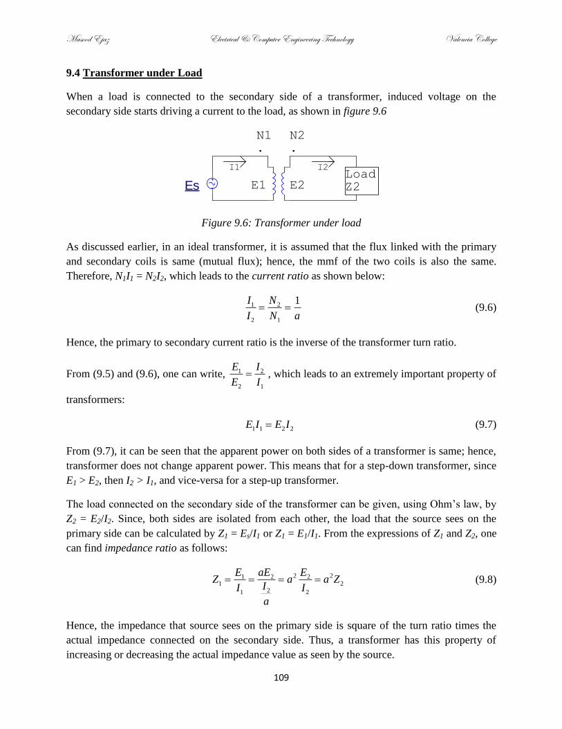
Masood Ejaz Electrical & Computer Engineering Technology Valencia College
109
9.4 Transformer under Load
When a load is connected to the secondary side of a transformer, induced voltage on the
secondary side starts driving a current to the load, as shown in figure 9.6
Figure 9.6: Transformer under load
As discussed earlier, in an ideal transformer, it is assumed that the flux linked with the primary
and secondary coils is same (mutual flux); hence, the mmf of the two coils is also the same.
Therefore, N1I1 = N2I2, which leads to the current ratio as shown below:
1 2
2 1
1I N
I N a (9.6)
Hence, the primary to secondary current ratio is the inverse of the transformer turn ratio.
From (9.5) and (9.6), one can write, 1 2
2 1
E I
E I , which leads to an extremely important property of
transformers:
1 1 2 2E I E I (9.7)
From (9.7), it can be seen that the apparent power on both sides of a transformer is same; hence,
transformer does not change apparent power. This means that for a step-down transformer, since
E1 > E2, then I2 > I1, and vice-versa for a step-up transformer.
The load connected on the secondary side of the transformer can be given, using Ohm’s law, by
Z2 = E2/I2. Since, both sides are isolated from each other, the load that the source sees on the
primary side can be calculated by Z1 = Es/I1 or Z1 = E1/I1. From the expressions of Z1 and Z2, one
can find impedance ratio as follows:
2 21 2 21 2
21 2
E aE EZ a a Z
II I
a
(9.8)
Hence, the impedance that source sees on the primary side is square of the turn ratio times the
actual impedance connected on the secondary side. Thus, a transformer has this property of
increasing or decreasing the actual impedance value as seen by the source.
Es
I2
N1.
I1
E1LoadZ2
N2.
E2

Masood Ejaz Electrical & Computer Engineering Technology Valencia College
110
Example # 9.2
An ideal transformer is connected to a 220V, 60Hz sinusoidal source. There are 100 turns on
the primary side and 3000 turns on the secondary side. A load is connected on the secondary
side which is drawing 2A current at a power factor of 80% lagging. Determine:
(i) Primary current
(ii) Secondary voltage
(iii) Load impedance
(iv) Individual components of the load
(v) Peak flux linked by the secondary winding
(vi) Phasor diagram of the system
Solution:
>> Es = E1 = 220V; f = 60Hz; N1 = 100; N2 = 3000; I2 = 2A; PF = 0.8;
(i) Primary current: I1 = N2*I2/N1 = 60A
(ii) Secondary Voltage: E2 = E1*N2/N1 = 6600V
(iii) Load impedance: |ZL| = E2/I2 = 3300
>> ∠ZL = cos-1
(0.8) = 36.870o
>> ZL = |ZL| cos(∠ZL) + |ZL| sin(∠ZL)i = 2640.0 + 1980.0i
(iv) RL = real(ZL) = 2640; XL = imag(ZL) = 1980.0
>> L = XL/(2*pi*f) = 5.2521H
(v) Peak flux linked with the secondary winding: = E2/(4.44*N2*f) = 8.2583mWb
(vi) Phasor diagram of the system:

Masood Ejaz Electrical & Computer Engineering Technology Valencia College
111
9.5 Impedance Shift
To emphasize on the important property of transformers that was discussed towards the end of
the last section, let’s reiterate it: the load impedance that the source on the primary side sees is
larger than the actual value for a step-down transformer (a > 1) and smaller than the actual value
for a step-up transformer (a < 1). The relationship between the voltage, current and impedance
ratios as given by (9.5), (9.6), and (9.8) enables us to create a single-loop circuit of a transformer
by either shifting secondary quantities to the primary side or primary quantities to the secondary
side. This is generally referred to as impedance shift. Note that this impedance shifting is
necessary in case if primary and secondary current (I1 and I2) and induced voltage values (E1 and
E2) are unknown. If any of those values are known then the circuit can be solved without
impedance shift.
Secondary side shifted to the primary side:
Observe a transformer circuit with primary and secondary line impedances, Z1 and Z2, and a load
impedance ZL, as shown in figure 9.7
Figure 9.7: An ideal transformer with line impedances and load impedance
To eliminate the transformer, the secondary side can be shifted to the primary with new
impedance values calculated according to the relationship given in (9.8). This will yield a circuit
with a single loop and calculation of different quantities can be done simply by using Ohm’s law.
The circuit corresponding to the secondary side shifted to the primary side is shown in figure 9.8
Figure 9.8: Secondary side reflected on the primary side
Z2
Es
I2
N1.
I1
E1
Z1
LoadZL
N2.
E2
I2'=I2/a = I1
Es
Z2'
I1
Z1
ZL'
+
EL' = a*EL
-

Masood Ejaz Electrical & Computer Engineering Technology Valencia College
112
Using (9.5), (9.6), and (9.8), the reflected values on the primary side, shown by prime (‘) in
figure 9.8, can be calculated as follows:
2
2 2
2
2 2
'
'
' /
'
L L
L L
Z a Z
Z a Z
I I a
E aE
(9.9)
If most of the quantities required are primary side quantities (input power, primary current etc.),
it will be convenient to shift secondary side to the primary and then solve the circuit.
Primary side shifted to the secondary side:
When primary side of the circuit from figure 9.7 is shifted to the secondary side, again, (9.5),
(9.6), and (9.8) are used to calculate the new shifted quantities, as shown by double prime (‘’) in
the reflected circuit shown in figure 9.9
Figure 9.9: Primary side reflected on the secondary side
The reflected values can be calculated using (9.5), (9.6), and (9.8) as follows:
2
1 1
1 1
'' /
''
'' /s s
Z Z a
I aI
E E a
(9.10)
If most of the quantities required are on the secondary side (load power, load current and voltage
etc.), it will be convenient to shift primary side to the secondary and then solve the circuit. This
way, secondary side quantities will stay the same.
I1''
ZLEs''
Z2
I2
Z1''
+
EL
-

Masood Ejaz Electrical & Computer Engineering Technology Valencia College
113
Note that since the power does not change on either side of the transformer, if load power is
required, you can shift the circuit on the primary side and calculate the power in the reflected
load value, which will be the same as the power in the actual load connected on the secondary
side.
Example # 9.3
An ideal transformer is connected to a 110V, 60Hz source. Turn ratio is 10. Primary line
reactance is 3 and resistance is 1. Secondary line reactance is 0.02 and resistance is
0.005. There is a capacitive load connected on the secondary with 0.1 resistance and 10mF
capacitance. Determine:
(i) Primary current
(ii) Secondary current
(iii) Load voltage
(iv) Active power of the load
(v) Reactive power of the load
Solution:
Since I1, I2, E1, and E2, all are unknown, we will have to reflect one side on another to solve
this problem. Let’s reflect the secondary side on the primary:
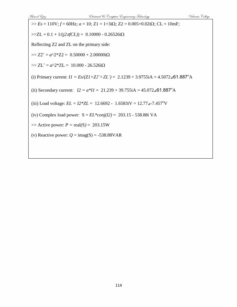
Masood Ejaz Electrical & Computer Engineering Technology Valencia College
114
>> Es = 110V; f = 60Hz; a = 10; Z1 = 1+3i; Z2 = 0.005+0.02i; CL = 10mF;
>>ZL = 0.1 + 1/(j2fCL)) = 0.10000 - 0.26526i
Reflecting Z2 and ZL on the primary side:
>> Z2’ = a^2*Z2 = 0.50000 + 2.00000i
>> ZL’ = a^2*ZL = 10.000 - 26.526i
(i) Primary current: I1 = Es/(Z1+Z2’+ZL’) = 2.1239 + 3.9755iA = 4.5072∠61.887oA
(ii) Secondary current: I2 = a*I1 = 21.239 + 39.755iA = 45.072∠61.887oA
(iii) Load voltage: EL = I2*ZL = 12.6692 - 1.6583iV = 12.77∠-7.457oV
(iv) Complex load power: S = EL*conj(I2) = 203.15 - 538.88i VA
>> Active power: P = real(S) = 203.15W
(v) Reactive power: Q = imag(S) = -538.88VAR

Masood Ejaz Electrical & Computer Engineering Technology Valencia College
115
PROBLEMS
1. An ideal transformer has 500 turns on the primary and 300 turns on the secondary. The
source produces a voltage of 600V (RMS) and load Z is a pure resistance of 12. Calculate:
(i) E2 (ii) I2 (iii) I1 (iv) Power delivered to the primary (W) (v) Power output from secondary
(W)
2. In problem 1, what is the impedance seen by the source?
3. A coil with an air core has a resistance of 14.7. When it is connected to a 42V, 60 Hz ac
source, it draws a current of 1.24A. Calculate:
(i) The impedance of the coil
(ii) Reactance of the coil and its inductance
(iii) Phase angle between the voltage and current
4. A 40F, 600V paper capacitor is available but we need one having rating of about 300F. It
is proposed to use a transformer to modify the 40F so that it appears as 300F. The
following transformer ratios are available: 120V/330V; 60V/450V; 480V/150V. Which
transformer is the most appropriate and what is the reflected value of the 40F capacitance?
To which side of the transformer should the 40F capacitor be connected?
5. An ideal transformer is connected to a 110V(rms), 60Hz source. Line impedance on the
primary is 4+5i and on the secondary side is 1+2i. A 1mF capacitor is connected as load
on the secondary side. Transformer has 100 turns on the primary side and 50 turns on the
secondary side. Calculate:
(i) Primary and secondary current
(ii) Active and reactive power supplied by the source.
(iii)Power factor of the source.

Masood Ejaz Electrical & Computer Engineering Technology Valencia College
116
Chapter 13 – Three-Phase Induction Machines
Three-phase induction machines are comprised of both three-phase induction motors and
generators. We will concentrate on mainly three-phase induction motors in this chapter. Three-
phase induction motors are AC motors with no DC power involved. They are widely used in
industry due to their simplicity, ruggedness, low price, and easy maintenance.
The construction of a three-phase induction motor is simple: three-phase windings are connected
to the stator that carry current to electromagnets to produce a three-phase magnetic field, and a
rotor is placed within the stator that is acted upon by the Lorentz force to rotate around an axis.
The difference between induction motors and DC motors that were discussed earlier is that the
rotor (armature) is not connected to any power supply that drives current through it. Rather,
current flows in the rotor due to the voltage that is induced in it due to the construction of rotor
and its interaction with the three-phase flux, as will be explained later in this chapter. Operation
of induction motors will be explained assuming the rotor to be a squirrel-cage rotor.
13.1 Force on a Conducting Ladder
Assume a ladder made out of a conducting material where current can easily flow, as shown in
figure 13.1. Observe that steps of the ladder are shorted out with the two sides of the ladder.
Imagine a situation where you are holding a permanent magnet over the ladder and moving it
along the ladder with some velocity ‘v’, as shown in the figure. When magnetic flux will link to
the ladder, and it will change due to the motion of the magnet, a voltage will induce in the steps
of the ladder in accordance with the Faraday’s law of electromagnetic induction.
Figure 13.1: Interaction between a magnet and a conducting ladder

Masood Ejaz Electrical & Computer Engineering Technology Valencia College
117
The direction of the induced voltage can be determined using the expression, eind = l.(v x B).
Assume that the current flow due to the induced voltage is in the positive-x direction. Hence,
length vector will have a direction ‘i’. Since magnet is moving in the positive-y direction, hence,
velocity vector of the moving magnet will have ‘j’ direction. Remember, in the equation to
calculate induced voltage, velocity vector is that of moving conductor, not moving magnet.
Hence, the velocity of the conductor will be taken as relative velocity with respect to the magnet.
When the conducting ladder is at rest, its magnitude of velocity will be the same as the
magnitude of velocity of the moving magnet, however, direction will be opposite. Hence, the
direction of the velocity of the conducting ladder will be in the ‘-j’ direction. Magnetic flux
density, B, is in the ‘–k’ direction. Hence, the direction of the induced voltage in the steps of the
conducting ladder will be i . (-j x –k) = i . i = 1. Therefore, our assumed direction of the flow of
current is correct, i.e. current will be coming out of the induced voltage in the positive-x
direction, and voltage induced will be positive in the positive-x direction.
As shown in figure 13.1, when the voltage is induced in the conducting ladder, current starts
flowing in it due to the short-circuit nature of conducting ladder steps. Current will flow out of
the step where voltage is induced and flow in the adjacent steps completing a loop. Now we have
a conductor carrying current interacting with magnetic field. What will be the result? Conducting
ladder will start experiencing Lorentz force, F = I (l x B). Since the direction of the length vector
is ‘i’ and the direction of magnetic flux density is ‘-k’, force on the ladder will be in the ‘j’
direction. Hence, if ladder is free to move, it will start moving in the same direction as the
moving magnet.
When ladder starts moving, the magnitude of the relative velocity between the moving magnet
and the moving ladder, |vladder – vmagnet|, becomes smaller. Hence, the Lorentz force on the ladder
also becomes smaller as well but since now ladder is already in motion, it does not require a
large force to keep itself in motion (remember our discussion of moving armature in a DC
motor). The conducting ladder will keep on accelerating until its velocity becomes quite close to
the velocity of the moving magnet, at which time, it will stop accelerating and starts moving with
a constant velocity. The ladder can never catch up with the moving magnet, i.e. their velocities
cannot become equal as there will always be some force required to overcome frictional forces
and keep ladder moving with a constant velocity. If ladder does catch up with the moving
magnet, the relative velocity will become zero and Lorentz force on the ladder will go down to
zero, and ladder will start decelerating. As soon it its velocity goes down, the relative velocity
becomes greater than zero and Lorentz force will start acting on it again.
With all this discussion about how a conducting ladder can accelerate under the influence of a
moving magnet, imagine if you bend the ladder upon itself to make a closed-loop, as shown in
figure 13.2, and use this loop as the armature of a motor which is free to rotate about an axis. If
this loop is acted upon by a moving magnetic field, it will start moving about the axis. This is the
principle of three-phase AC induction motors, and the armature crafted in such a way is called a
squirrel-cage rotor.

Masood Ejaz Electrical & Computer Engineering Technology Valencia College
118
Figure 13.2: Squirrel-cage rotor
13.2 Rotating Magnetic Field
A three-phase induction motor has three-phase electromagnets on its stator. Each phase is
connected to its corresponding electromagnet, as shown in figure 13.2.
Figure 13.2: Three phases connected to three electromagnets (two poles per magnet)
As three-phase current flows in the windings of electromagnets, a three-phase flux is produced.
Like three-phase current, this three-phase flux is also 120o apart from each other. At each instant
of time, the resultant flux from the three phases adds up in such a way that it points to one
direction. Over one input cycle (360o), the resultant flux also rotates around one cycle. In this
way, a three-phase field produces a rotating magnetic field. This is shown in figure 13.3

Masood Ejaz Electrical & Computer Engineering Technology Valencia College
119
Figure 13.3: (a) Instantaneous values of three-phase currents (b)-(g) Resultant flux at instances 1 through 6 as
shown in (a)
(b)
(c)
(d)
(a)
(e)
(f)
(g)

Masood Ejaz Electrical & Computer Engineering Technology Valencia College
120
The speed with which flux is rotating is called synchronous speed. Synchronous speed (ns)
depends on the input voltage frequency (f) and number of poles per phase (P). Mathematically, it
is given by the following equation:
120(rpm)s
fn
P (13.1)
Hence, for two poles per phase, as shown in figure 13.2, and with an input frequency of 60Hz,
the synchronous speed will be 3600rpm or 60Hz, i.e. one complete input cycle will produce one
complete rotating cycle of the flux.
It is possible to create a group of poles per phase, more than two poles. This type of stator
arrangement will produce a flux with synchronous speed less than the input frequency. For an n-
group per phase stator, the groups are connected in series in such a way that when phase current
flows through them, it creates n alternating N-S poles. Figure 13.4 shows a stator with four and
eight groups of poles.
Figure 13.4: (a) Four poles per phase (b) Eight poles per phase
It is easy to change the direction of the revolving flux by changing the sequence of three phases
connected to the electromagnet on the stator. If sequence ABC is producing a revolving flux in
counter-clockwise direction, changing the sequence to ACB will make the flux revolve in
clockwise direction. This can be used to apply electrical braking as well as changing the
direction of rotation of the rotor, as will be discussed next.
(a)
(b)

Masood Ejaz Electrical & Computer Engineering Technology Valencia College
121
13.3 Working of a Squirrel-cage Three-Phase Induction Motor
The squirrel-cage rotor is placed in the center of the three-phase stator of the induction motor.
The rotor is free to rotate about its axis. When the three-phase current produces a three-phase
flux, the resultant of which revolves around with synchronous speed, it induces a voltage in the
steps of the squirrel-cage rotor in a similar way as the moving magnet induces voltage in the
conducting ladder. This induced voltage drives a current in the squirrel-cage rotor. The squirrel-
cage rotor experiences Lorentz force due to the interaction between the revolving magnetic field
and the current that is flowing in it, which produces a torque that starts moving the rotor in the
same direction as the direction of the revolving magnetic field.
The initial voltage induced in the rotor when it is at rest is quite large, since the magnitude of the
relative velocity of the rotor with respect to the revolving magnetic flux is maximum. This large
voltage runs a large starting current in the rotor, due to which it experiences a large Lorentz force
which creates a large torque to move the rotor rapidly from its resting position. Once it starts
rotating, magnitude of the relative velocity becomes smaller, which in turns results in a smaller
induced voltage, which runs smaller current in the rotor. The Lorentz force goes down, since the
value of the current is smaller and hence, torque becomes smaller as well. But since now the
rotor is moving, it does not require as large of a force and torque to accelerate. The rotor keeps
on accelerating until it reaches very close to the synchronous speed and then it starts rotating
with a constant velocity. The difference between the synchronous speed (ns) and the rotor speed
(n) is called slip speed. There is also a parameter, called slip, which is used to measure the slip
speed with respect to the synchronous speed, and it is given as follows:
s
s
n ns
n
(13.2)
At no load, slip is around 0.1% since rotor speed is practically equal to the synchronous speed.
When the motor is connected to a load, it starts slowing down. When rotor speed decreases, slip
increases, which results in the increase of induced voltage in rotor. When induced voltage is
increased, short-circuit current in the rotor is increased, which results in a larger Lorentz force,
and hence, larger torque. The speed of the rotor keeps on decreasing and rotor torque keeps on
increasing as long as it becomes equal to the torque exerted by the load on the rotor. When the
load torque becomes equal to the rotor torque, motor starts rotating at a constant speed, which is
a little less than no-load speed. Under normal loads, induction motor runs very close to the
synchronous speed. At full-load, the slip for large motors (1MW and more) rarely exceeds 0.5%
and for smaller machines (10KW or less), it seldom exceeds 5%. That is why induction motors
are considered to be constant speed machines. Also, since they never actually run at synchronous
speed, sometimes they are also referred to as asynchronous machines.
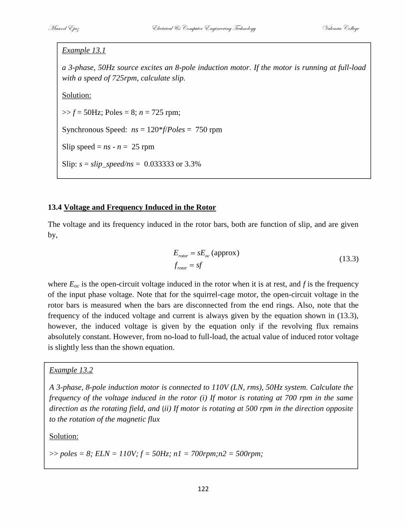
Masood Ejaz Electrical & Computer Engineering Technology Valencia College
122
13.4 Voltage and Frequency Induced in the Rotor
The voltage and its frequency induced in the rotor bars, both are function of slip, and are given
by,
(approx)rotor oc
rotor
E sE
f sf
(13.3)
where Eoc is the open-circuit voltage induced in the rotor when it is at rest, and f is the frequency
of the input phase voltage. Note that for the squirrel-cage motor, the open-circuit voltage in the
rotor bars is measured when the bars are disconnected from the end rings. Also, note that the
frequency of the induced voltage and current is always given by the equation shown in (13.3),
however, the induced voltage is given by the equation only if the revolving flux remains
absolutely constant. However, from no-load to full-load, the actual value of induced rotor voltage
is slightly less than the shown equation.
Example 13.1
a 3-phase, 50Hz source excites an 8-pole induction motor. If the motor is running at full-load
with a speed of 725rpm, calculate slip.
Solution:
>> f = 50Hz; Poles = 8; n = 725 rpm;
Synchronous Speed: ns = 120*f/Poles = 750 rpm
Slip speed = ns - n = 25 rpm
Slip: s = slip_speed/ns = 0.033333 or 3.3%
Example 13.2
A 3-phase, 8-pole induction motor is connected to 110V (LN, rms), 50Hz system. Calculate the
frequency of the voltage induced in the rotor (i) If motor is rotating at 700 rpm in the same
direction as the rotating field, and (ii) If motor is rotating at 500 rpm in the direction opposite
to the rotation of the magnetic flux
Solution:
>> poles = 8; ELN = 110V; f = 50Hz; n1 = 700rpm;n2 = 500rpm;

Masood Ejaz Electrical & Computer Engineering Technology Valencia College
123
13.5 Line Current under Different Conditions
At no load, the stator current (line current) is about 0.3 to 0.5 times the full-load current. This
current is mainly required to produce magnetic flux that links with the rotor (reactive power),
and to compensate for stator winding loss and small frictional and windage losses in the rotor
(active power). Since there is no output power at no-load, efficiency is zero. The power factor at
no load is low; it ranges from 20% for small machines and 5% for large machines
When the motor is loaded, rotor current increases and it produces its own magnetic field. This
magnetic field interacts with the stator magnetic field and the mutual flux pattern changes a little.
In addition to mutual flux, stator and rotor produce leakage flux as well. The stator current
increases to compensate for the reactive power required for these three types of flux. In addition
to a little increase in the reactive power, the active power increased a lot to convert electrical
power into mechanical to support the load. Hence, the stator current increases quite a bit to
compensate the increase of both reactive and active powers. At full-load, the power factor of the
motor ranges from 80% for smaller machines to 90% for larger machines. Efficiency of the
motor is very high and can go up to 98% for larger machines.
When rotor is locked (rotor is at rest), very large voltage is induced in the rotor bars and starting
current is extremely large; 5 to 6 times the full-load current. This increases the rotor copper loss
from 25 to 36 times the loss at full-load (I2R). The leakage flux of the stator and rotor also
increase. Although the output power of the locked-rotor is zero but the large copper loss in
addition with the increase of reactive power require large line current. Due to the large power
loss, the rotor should never remain locked for more than a few seconds.
The full-load current of a three-phase induction motor is approximately given by the following
equation:
Synchronous speed: ns = 120*f/poles = 750 rpm
(i) Slip: s = (ns-n1)/ns = 0.066667
Frequency of the induced voltage: fr = s*f = 3.3333 Hz
(ii) Slip: s = (ns-(-n2))/ns = 1.667 (If motor speed is in the opposite direction to ns, take it as
negative)
Note: A slip > 1 represents that electrical braking is applied on the rotor and it is slowing
down
Frequency of the induced voltage: fr = s*f = 83.333 Hz
Note: When motor is at rest (locked rotor), speed is 0 and slip is 1. Frequency of the induced
voltage will then be equal to the line frequency.

Masood Ejaz Electrical & Computer Engineering Technology Valencia College
124
600 h
LL
PI
E (13.4)
where Ph is the output horsepower of the motor and ELL is line-to-line input voltage.
13.6 Power Flow in a Three-Phase Induction Motor
Three phase active power enters into the stator of the motor, which can be given by,
3 cos( )LN LPin V I (13.5)
There are two losses in the stator; stator copper loss and stator core loss. Copper loss is due to
the heat dissipated due to the resistance of the stator winding when current flows through it. Core
loss, which is also called iron loss, is comprised of the hysteresis and eddy current loss in the
iron core. Copper loss is calculated through the usual I2R equation:
23SCL L statorP I R (13.6)
Example 13.3
If starting current (locked rotor) of an induction motor is five times the full-load current and
no-load current is half of the full-load current of a 1000hp, 120V(phase) motor, calculate full-
load, no-load, and locked rotor currents. Also calculate the apparent power drawn at full-
load.
Solution:
>> Motor_hp = 1000; (Make sure to convert it into hp if given in watt)
>> ELN = 120V; ELL = sqrt(3)*120; ((13.4) calls for line-to-line voltage)
Full-load current: IFL = 600*Motor_hp/ELL = 2886.8A or 2.886 KA
No-load current: INL = 0.5*IFL = 1443.4A or 1.443 KA
Locked-rotor current: ILocked_rotor = 5*IFL = 14433.75673 or 14.433KA
Apparent power at full-load: S = 3*ELN*IFL = 1039230.48454 VA or 1.039 MVA (Assuming
RMS values of currents and voltages)

Masood Ejaz Electrical & Computer Engineering Technology Valencia College
125
Core loss is generally given. At this point, the remaining power is transmitted to the rotor
through the air gap between the rotor and the stator. Hence, it is called air gap power or active
rotor power,
r in SCL coreP P P P (13.7)
The first loss that is considered in the rotor is rotor copper loss. This is calculated as a product of
slip and the rotor power,
RCL rP sP (13.8)
where slip is calculated using (13.1) and (13.2). The power available after this point is called
induced or mechanical power,
(1 )M r RCL r r rP P P P sP s P (13.9)
The next power loss is due to friction and windage, which is usually given. The remaining power
is the output or shaft power available to move the load.
&out M F WP P P (13.10)
If frictional and windage losses are negligible then mechanical power is equal to the output or
shaft power. Also, if core, windage, and frictional losses are not given but one can calculate other
losses and the output power then core, windage, and frictional losses can be calculated by
subtracting other losses and the output power from the input power.
Efficiency of a motor is given by the ratio of the output to the input power, as discussed earlier in
section 6.4. Figure 13.5 shows the active power flow routine as discussed in this section.
Figure 13.5: Power Flow in a Three-Phase Induction Motor

Masood Ejaz Electrical & Computer Engineering Technology Valencia College
126
13.7 Motor Torque
Output torque of the motor is given by,
9.55 outPT
n (13.11)
If frictional and windage losses are negligible then output power and mechanical power will be
approximately equal and the torque of the motor will be given by,
9.55 9.55(1 ) 9.55
(1 )
M r r
s s
P s P PT
n n s n
(13.12)
Remember, the unit of torque is Newton-meter (N.m)
13.8 Speed-Torque Relationship
The torque developed by a motor depends upon its speed but the relationship between the two is
not very easy to express in a closed-form equation. Instead, figure 13.6 shows the torque vs.
speed relationship of a three-phase induction motor with nominal full-load torque of T.
Figure 13.6: Speed-Torque Relationship of a 3-Phase Squirrel-Cage Motor

Masood Ejaz Electrical & Computer Engineering Technology Valencia College
127
As shown in the figure, the starting torque is 1.5 times and the maximum torque, also called
breakdown torque, is 2.5 times the nominal full-load torque. Pull-up torque is the minimum
torque developed by the motor when it is accelerating from rest to the breakdown torque.
As discussed earlier, when a load is attached to a motor, it slows down, which results in a drop of
the counter EMF, which increases the rotor current, which in turns increases the Lorentz force on
the rotor, which results in a greater torque developed by the rotor. The torque of the motor
increases until it becomes equal to the torque required by load, at which point motor, once again,
starts spinning with a constant speed, which may be slightly less than the speed without load. If
the connected load exerts a very high torque that it exceeds the breakdown torque, the motor will
quickly stop.
Smaller motors (15hp or less) develop their breakdown torque at a speed of about 80% of the
synchronous speed (shown as nd in figure 13.6). Large motors (1500hp or more) attain their
breakdown torque at about 98% of the synchronous speed.
Example 13.4
A 3-phase, 4 KV (LL, rms), 60 Hz squirrel-cage induction motor draws a current of 385A and
a total active power of 2344 KW when operating at full-load. It has 10 poles per phase. Speed
of the rotor is 709.2 rpm. Stator resistance per phase is 0.05. The total iron losses are
23.4KW and windage and friction losses are 12KW. Calculate:
(i) The power factor at full-load; (ii) The active power supplied to the rotor; (iii) Total copper
losses in the rotor; (iv) Efficiency of the motor; (v) Output torque of the motor
Solution:
>> ELL = 4000V; ELN = ELL/sqrt(3); f = 60Hz; IFL = 385A; Pmotor = 2344KW; poles = 10; n
= 709.2rpm; Rs = 0.05; iron_loss = 23.4KW; friction_loss = 12KW;
(i) PF at full-load:
Apparent power: S = 3*ELN*IFL = 2667358.24366 VA = 2667.358KVA
Power factor: PF = Pmotor/S = 0.87877 or 87.877% lagging, since motor is mostly inductive.
(ii) The active power supplied to the rotor:
Stator copper loss: Pscl = 3*IFL2*Rs = 22233.75000 W = 22.233KW
Rotor power: Pr = Pmotor - Pscl - iron_loss = 2298366.25000W = 2298.366KW
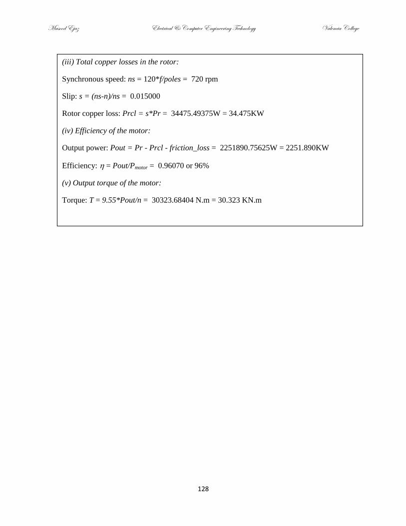
Masood Ejaz Electrical & Computer Engineering Technology Valencia College
128
(iii) Total copper losses in the rotor:
Synchronous speed: ns = 120*f/poles = 720 rpm
Slip: s = (ns-n)/ns = 0.015000
Rotor copper loss: Prcl = s*Pr = 34475.49375W = 34.475KW
(iv) Efficiency of the motor:
Output power: Pout = Pr - Prcl - friction_loss = 2251890.75625W = 2251.890KW
Efficiency: = Pout/Pmotor = 0.96070 or 96%
(v) Output torque of the motor:
Torque: T = 9.55*Pout/n = 30323.68404 N.m = 30.323 KN.m

Masood Ejaz Electrical & Computer Engineering Technology Valencia College
129
PROBLEMS
1. Calculate the synchronous speed of a 3-phase, 12-pole induction motor that is excited by a
60-Hz source. What is the nominal speed (n) if slip at full-load is 6%?
2. A 3-phase, 6-pole induction motor is connected to a 60-Hz supply. The voltage induced in
the rotor bars is 4V when the rotor is locked (open-circuit voltage). If the motor turns in the
same direction as flux, calculate the approximate voltage induced and its frequency at (i) 300
rpm, and (ii) 1000 rpm
3. The no-load current of a 75KW, 4000V, 3-phase, 900rpm, 60HZ induction motor is one-third
and starting current is six times the full-load current. Calculate (i) the approximate values of
full-load current, starting current, and no-load current (ii) the output torque, synchronous
speed, and rotor power (air gap power) given that slip is 2%.
4. A 3-phase, 75 hp, 400 V induction motor has a full load efficiency of 91% and a power factor
of 83% lagging. Calculate the nominal current per phase.
5. A 3-phase 5KV (L-L), 8-pole, 60Hz, squirrel-cage induction motor draws a current of 400A
and total active power of 3.3255 MW when operating at full-load. Full-load speed is 890
rpm. Resistance of stator winding is 0.05 per phase and it is connected in wye. Total iron
losses are 30KW and windage and friction losses are 20KW. Calculate: (i) Power factor at
full load, (ii) Active power supplied to the rotor, (iii) Total copper losses of rotor (I2R), (iv)
Output power, (v) Torque, and (vi) Efficiency.

Masood Ejaz Electrical & Computer Engineering Technology Valencia College
130
Chapter 16 – Synchronous Generators
The primary way to produce electrical power for consumption is through synchronous AC
generators. They can convert mechanical energy into electrical in excess of 1.5GW. The basic
principle is the same as discussed under three-phase systems; a moving magnet creates a time-
varying flux which links with the three-phase windings and induces voltage in them. For bigger
synchronous generators with high power rating, field is produced by a set of moving magnetic
poles, which makes the rotor of the machine, and three-phase windings in which voltage is
induced are stationary and make stator of the machine. This is for the obvious reason of not
using any moving parts (slip rings, carbon brushes etc.) between the load and the generator, since
the generated voltage is very high, which produces a very large power when connected to the
load. There can also be synchronous generators with stationary magnetic field and moving three-
phase winding with one slip-ring connected to each phase. These machines are usually used for
low-voltage and low-power generation. The three-phase synchronous generators with three-
phase winding on the stator and magnetic flux produced by the rotor are also called alternators.
Synchronous generators are called synchronous due to the fact that the induced voltage
frequency is synchronized (locked) to the speed of rotation of the magnetic field (rotor).
16.1 Number of Poles
The number of poles on the rotor in a synchronous generator depends upon the speed of rotation
and the required induced voltage frequency. In general, the frequency of the induced voltage (in
Hz) is given by the following equation:
120
npf (16.1)
where n is the speed of rotation of the rotor in rpm and p is the number of poles. Hence, to
produce a 60-Hz voltage waveform from a 2-pole (N-S) generator, it must be rotated at 3600rpm.
Example 16.1: It is required to produce the frequency of the induced voltage of a synchronous
generator to be 60Hz using an 8-pole rotor. How fast the rotor should be rotated?
Solution:
f = 60Hz; poles = 8;
Since, f = n*poles/120 n = 120*f/poles = 900 rpm
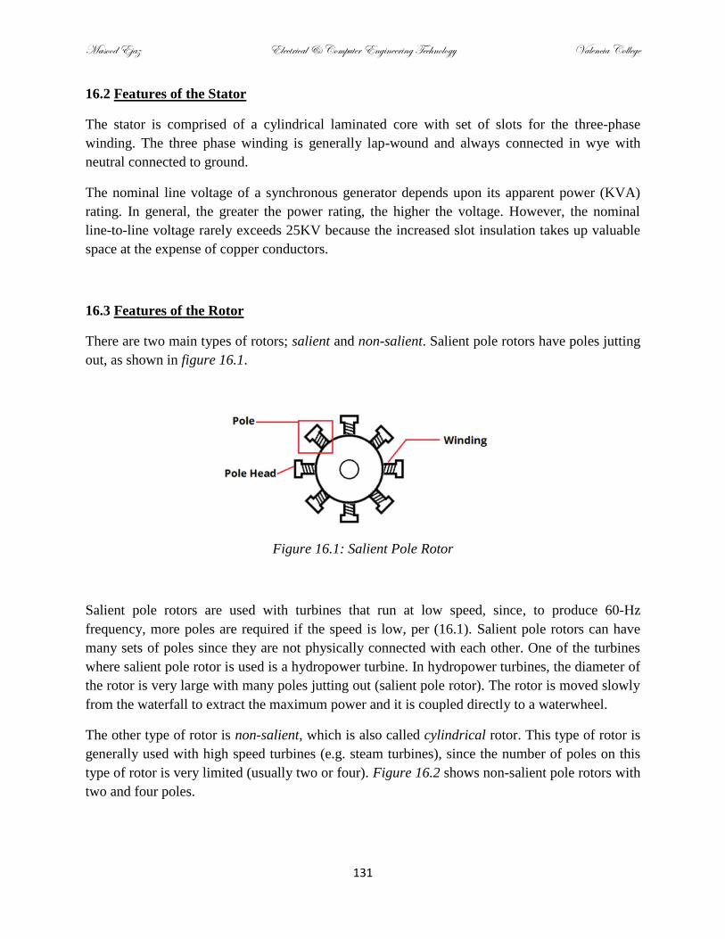
Masood Ejaz Electrical & Computer Engineering Technology Valencia College
131
16.2 Features of the Stator
The stator is comprised of a cylindrical laminated core with set of slots for the three-phase
winding. The three phase winding is generally lap-wound and always connected in wye with
neutral connected to ground.
The nominal line voltage of a synchronous generator depends upon its apparent power (KVA)
rating. In general, the greater the power rating, the higher the voltage. However, the nominal
line-to-line voltage rarely exceeds 25KV because the increased slot insulation takes up valuable
space at the expense of copper conductors.
16.3 Features of the Rotor
There are two main types of rotors; salient and non-salient. Salient pole rotors have poles jutting
out, as shown in figure 16.1.
Figure 16.1: Salient Pole Rotor
Salient pole rotors are used with turbines that run at low speed, since, to produce 60-Hz
frequency, more poles are required if the speed is low, per (16.1). Salient pole rotors can have
many sets of poles since they are not physically connected with each other. One of the turbines
where salient pole rotor is used is a hydropower turbine. In hydropower turbines, the diameter of
the rotor is very large with many poles jutting out (salient pole rotor). The rotor is moved slowly
from the waterfall to extract the maximum power and it is coupled directly to a waterwheel.
The other type of rotor is non-salient, which is also called cylindrical rotor. This type of rotor is
generally used with high speed turbines (e.g. steam turbines), since the number of poles on this
type of rotor is very limited (usually two or four). Figure 16.2 shows non-salient pole rotors with
two and four poles.

Masood Ejaz Electrical & Computer Engineering Technology Valencia College
132
Figure 16.2: Cylindrical Rotors
Figure 16.3 shows cross-section of synchronous generators with both types of rotors.
Figure 16.3: Synchronous Generators with Salient and Non-Salient Rotors
Example 16.2: A waterfall is rotating a salient pole rotor with speed of 100 rpm. If the required
output frequency is 60Hz, how many poles will be required on the rotor?
Solution:
f = 60Hz; n = 100rpm;
Since, f = n*poles/120 poles = 120*f/n = 72 or 36 pairs of N-S
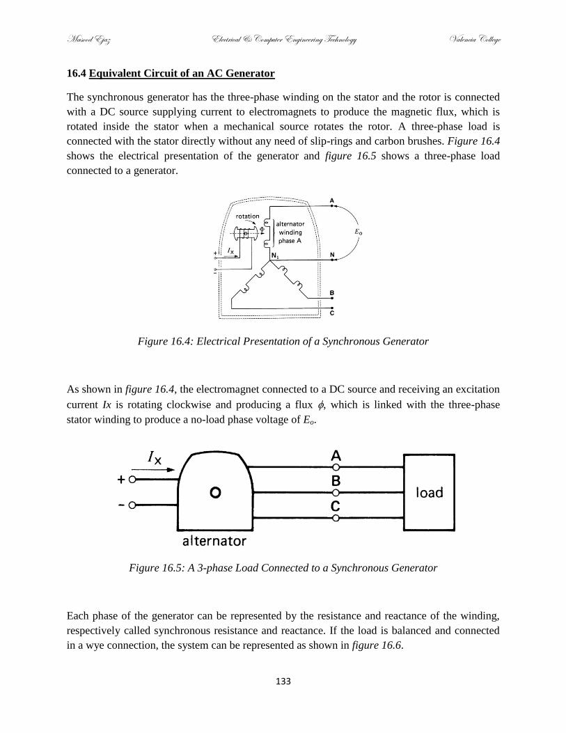
Masood Ejaz Electrical & Computer Engineering Technology Valencia College
133
16.4 Equivalent Circuit of an AC Generator
The synchronous generator has the three-phase winding on the stator and the rotor is connected
with a DC source supplying current to electromagnets to produce the magnetic flux, which is
rotated inside the stator when a mechanical source rotates the rotor. A three-phase load is
connected with the stator directly without any need of slip-rings and carbon brushes. Figure 16.4
shows the electrical presentation of the generator and figure 16.5 shows a three-phase load
connected to a generator.
Figure 16.4: Electrical Presentation of a Synchronous Generator
As shown in figure 16.4, the electromagnet connected to a DC source and receiving an excitation
current Ix is rotating clockwise and producing a flux , which is linked with the three-phase
stator winding to produce a no-load phase voltage of Eo.
Figure 16.5: A 3-phase Load Connected to a Synchronous Generator
Each phase of the generator can be represented by the resistance and reactance of the winding,
respectively called synchronous resistance and reactance. If the load is balanced and connected
in a wye connection, the system can be represented as shown in figure 16.6.
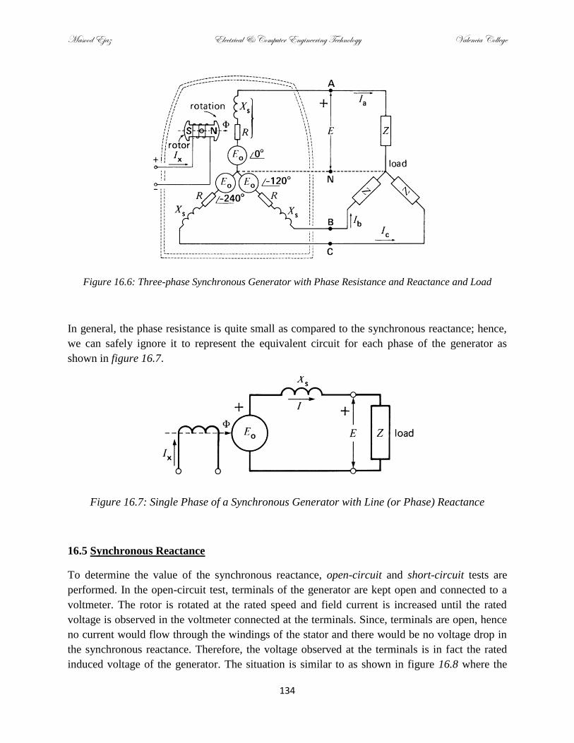
Masood Ejaz Electrical & Computer Engineering Technology Valencia College
134
Figure 16.6: Three-phase Synchronous Generator with Phase Resistance and Reactance and Load
In general, the phase resistance is quite small as compared to the synchronous reactance; hence,
we can safely ignore it to represent the equivalent circuit for each phase of the generator as
shown in figure 16.7.
Figure 16.7: Single Phase of a Synchronous Generator with Line (or Phase) Reactance
16.5 Synchronous Reactance
To determine the value of the synchronous reactance, open-circuit and short-circuit tests are
performed. In the open-circuit test, terminals of the generator are kept open and connected to a
voltmeter. The rotor is rotated at the rated speed and field current is increased until the rated
voltage is observed in the voltmeter connected at the terminals. Since, terminals are open, hence
no current would flow through the windings of the stator and there would be no voltage drop in
the synchronous reactance. Therefore, the voltage observed at the terminals is in fact the rated
induced voltage of the generator. The situation is similar to as shown in figure 16.8 where the

Masood Ejaz Electrical & Computer Engineering Technology Valencia College
135
three voltmeters are measuring the line-to-line terminal voltages. Although, the figure shows
measurement of the line-to-line terminal voltage but to measure the induced phase voltage, line-
to-neutral terminal voltage is used. Hence, if line-to-line is given, divide it by the square root of 3
to get line-to-neutral voltage.
Figure 16.8: Open-Circuit Test to determine Voc
Next, terminals of the generator are shorted out through an ammeter. The rotor is rotated at the
rated speed and same field current is given to the electromagnet in the rotor. This would produce
the same flux as under the open-circuit test and the induced voltage would also be the same. The
current passing through the ammeter is noted. This is shown in figure 16.9.
Figure 16.9: Short-Circuit Test to determine Isc
The synchronous reactance can now be calculated by taking the ration of the open-circuit voltage
to the short-circuit current using Ohm’s law:

Masood Ejaz Electrical & Computer Engineering Technology Valencia College
136
oc
sc
VXs
I (16.2)
16.6 Synchronous Generator Under Load
Two different types of loads can be connected to a synchronous generator; isolated load, and
infinite bus.
Isolated Load: When a three-phase load (mostly balanced) is connected to the terminals of the
generator, it is referred to as an isolated load.
Example 16.3: A 3-phase synchronous generator produces an open-circuit voltage of 7000V
(LL) when field excitation current is 52A. The terminals of the generator are then shorted and
three line currents are found to be 800A for the same excitation current. Calculate:
(i) Synchronous reactance Xs per phase (ii) If a balanced load of 5 resistors is connected to
the terminals, determine the load current and voltage.
Solution:
(i) Synchronous reactance Xs per phase
>> EocLL = 7000V; Isc = 800A; EocLN = EocLL/sqrt(3) = 4041.5V;
Magnitude of the reactance: Xs = EocLN/Isc = 5.0581
(ii) If a balanced load of 3 resistors is connected to the terminals, determine the load current
and voltage.
>> Xs = j5.0581; RL = 5;
Current in the circuit: I = EocLN/(RL + Xs)
= 399.48 - 404.12i A = 568.24∠-45.331oA
Load Current: E= I*RL = 1997.4 - 2020.6i V
= 2841.2∠-45.331oV
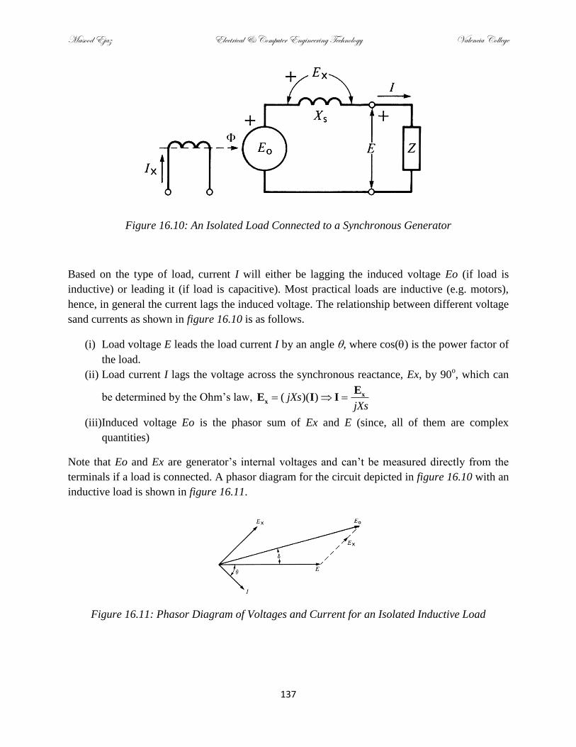
Masood Ejaz Electrical & Computer Engineering Technology Valencia College
137
Figure 16.10: An Isolated Load Connected to a Synchronous Generator
Based on the type of load, current I will either be lagging the induced voltage Eo (if load is
inductive) or leading it (if load is capacitive). Most practical loads are inductive (e.g. motors),
hence, in general the current lags the induced voltage. The relationship between different voltage
sand currents as shown in figure 16.10 is as follows.
(i) Load voltage E leads the load current I by an angle , where cos() is the power factor of
the load.
(ii) Load current I lags the voltage across the synchronous reactance, Ex, by 90o, which can
be determined by the Ohm’s law, ( )( )jXsjXs
xx
EE I I
(iii)Induced voltage Eo is the phasor sum of Ex and E (since, all of them are complex
quantities)
Note that Eo and Ex are generator’s internal voltages and can’t be measured directly from the
terminals if a load is connected. A phasor diagram for the circuit depicted in figure 16.10 with an
inductive load is shown in figure 16.11.
Figure 16.11: Phasor Diagram of Voltages and Current for an Isolated Inductive Load

Masood Ejaz Electrical & Computer Engineering Technology Valencia College
138
If the isolate load is capacitive in nature, load current will lead the load voltage by an angle . Ex
will still lead the load current, since Xs is pure inductance, and surprisingly, the magnitude of the
induced voltage will be smaller than the magnitude of the load voltage, although, the higher
terminal voltage does not yield any more power. The corresponding phasor diagram is shown in
figure 16.12.
Figure 16.2: Phasor Diagram of Voltages and Current for an Isolated Capacitive Load
Infinite Bus: When a synchronous generator is connected to a power grid to which many other
generators are also connected, the load is referred to as infinite bus. All generators connected to
an infinite bus appear to be in parallel to each other. Infinite bus is such a powerful system that it
imposes its voltage and frequency to any generator that is connected to it. When a generator is
connected to an infinite bus, it becomes part of the power system and starts delivering power to
thousands of loads connected to the power grid. Hence, it is impossible to specify nature of a
load connected to the terminals of any specific generator.
As soon as a generator is connected to the infinite bus, its terminal voltage assumes the bus
voltage and induced voltage also becomes equal to the terminal voltage. Under this condition, no
current flows from the generator towards the bus (Ohm’s law) and it does not contribute in any
power flow. The generator is said to be in the floating state.
Figure 16.3: Generator in the Floating State
To make generator contribute power to the infinite bus, two parameters of the synchronous
generator can be changed; field current Ix and rotor speed.

Masood Ejaz Electrical & Computer Engineering Technology Valencia College
139
When field current Ix will increase, field flux will increase, which will result in the increase of
the induced voltage Eo. Now, the current will start flowing from the generator to the infinite bus
and there will be some voltage drop in Xs. However, the synchronous reactance is much smaller
than the infinite bus load, therefore, both the induced voltage and the voltage across the infinite
bus (terminal voltage) will be in phase and the current will be lagging all three voltages in the
circuit by 90o, due to that fact that it would be lagging Ex by 90
o (pure inductance) and Ex is in
phase with Eo and E. The current can easily be calculated using Ohm’s law (s
IjX
Eo E). This
situation is shown in figure 16.4.
Figure 16.4: Over-excitation of the Generator
Once again, remember that all voltages and currents here are complex quantities, so do not
attempt to perform mathematical operation on their magnitudes only.
Since, current is lagging the induced voltage, the only power flow in this case will be the reactive
power flow and no real or active power will be delivered by the generator to the bus,
3 cos(90) 0W
3 sin(90) 3 VAR
o
o o
P E I
Q E I E I
(16.3)
Under this condition, the generator will see the load as being inductive, since current is lagging
the induced voltage by 90o. This condition is called over-excitation of the generator.
If Ix is reduced below its rated value, flux will be reduced, and Eo will be decreased. Now, Eo
will become less than the terminal voltage E. Hence, the current direction will be reversed; bus
will start supplying current to the generator or the generator will see the load as a capacitive load.
Current will lead both Eo and E by 90o but it will still lag Ex by 90
o, since it is pure inductor. The
power flow in this case will still be reactive. The power, which is flowing from the bus to the
generator, will partially magnetize the generator’s field; rest will come from the field current Ix.
3 cos( 90) 0W
3 sin( 90) 3 VAR
o
o o
P E I
Q E I E I
(16.4)
This condition is called under-excitation of the generator. The corresponding circuit and phasor
diagram are shown in figure 16.5.

Masood Ejaz Electrical & Computer Engineering Technology Valencia College
140
Figure 16.5: Under-excitation of the Generator
Under both over- and under-excitation conditions, not real power is delivered by the generator.
Now, let’s discuss how a generator will deliver real or active power to the infinite bus. This
happens when the speed of the rotor of the generator is increased by changing the mechanical
torque of the turbine. The effect of increasing the mechanical torque of the turbine to increase the
rotor speed is that the rated induced voltage will be achieved earlier than before, thus creating a
phase difference between Eo and E, although their magnitudes will remain same. The phase
difference between Eo and E is called the torque angle, . Now, the generator will provide active
power to the bus as well as some reactive power. The corresponding circuit and phasor diagram
are shown figure 16.6.
Figure 16.6: Torque of the Turbine is increased to deliver Real Power
If torque of the turbine will keep on increasing, torque angle will keep on increasing and
generator will keep providing more active power to the infinite bus. When mechanical power of
the turbine will become equal to the electrical power delivered by the generator to the bus, torque
angle will become almost constant (instead of changing) and turbine will not accelerate anymore.
At this time, the generator will be contributing a lot more active power to the bus as compared to
the reactive power.
Once again, makes sure not to get confused while doing calculation of different quantities in the
circuit. All quantities are complex. For example, the magnitudes of the induced voltage and
terminal voltage are same in figure 16.6 but Eo also has a phase. Therefore, when calculating the
current in the circuit, both magnitude and phase of each quantity must be considered.

Masood Ejaz Electrical & Computer Engineering Technology Valencia College
141
If both field current and torque of the turbine will increase, the magnitude of Eo will increase as
well as the torque angle. Both real and reactive powers will be supplied by the generator to the
infinite bus under that condition.
Example 16.4: A 3-phase synchronous generator is connected to a power grid. The synchronous
reactance (per phase) of the generator is 9. If induced voltage is 12KV(LL), Calculate the
active power that machine delivers when the torque angle is 30o.
Solution:
Assume all values to be RMS.
>> = 30o; Xs = 9i; |EoLN| = 12000/sqrt(3)V = 6928.2V; E = |EoLN|
EoLN = 6928.2cos() + i 6928.2sin()= 6000.0 + 3464.1i V
I = (EoLN - E)/Xs = 384.90 + 103.13i A
Total complex power delivered:
S = 3*EoLN*conj(I)
S = 8000000.00000 + 2143593.53945i VA
Therefore, total active power delivered is 8MW
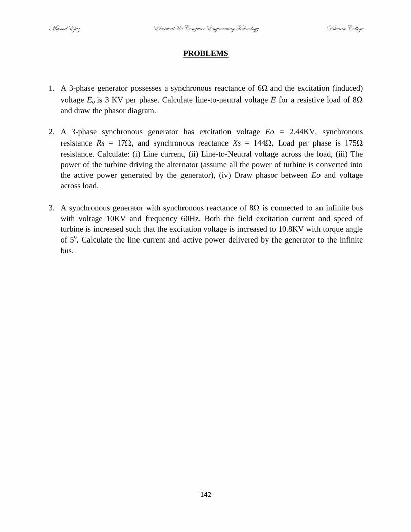
Masood Ejaz Electrical & Computer Engineering Technology Valencia College
142
PROBLEMS
1. A 3-phase generator possesses a synchronous reactance of 6and the excitation (induced)
voltage Eo is 3 KV per phase. Calculate line-to-neutral voltage E for a resistive load of 8
and draw the phasor diagram.
2. A 3-phase synchronous generator has excitation voltage Eo = 2.44KV, synchronous
resistance Rs = 17, and synchronous reactance Xs = 144. Load per phase is 175
resistance. Calculate: (i) Line current, (ii) Line-to-Neutral voltage across the load, (iii) The
power of the turbine driving the alternator (assume all the power of turbine is converted into
the active power generated by the generator), (iv) Draw phasor between Eo and voltage
across load.
3. A synchronous generator with synchronous reactance of 8 is connected to an infinite bus
with voltage 10KV and frequency 60Hz. Both the field excitation current and speed of
turbine is increased such that the excitation voltage is increased to 10.8KV with torque angle
of 5o. Calculate the line current and active power delivered by the generator to the infinite
bus.


