1

Blueprints for ETL workflows

Panos Vassiliadis1, Alkis Simitsis2, Manolis Terrovitis2, Spiros Skiadopoulos2

1 University of Ioannina, Dept. of Computer Science, 45110, Ioannina, Greece

pvassil@cs.uoi.gr 2 National Technical University of Athens, Dept. of Electrical and Computer Eng.,

Computer Science Division, Iroon Polytechniou 9, 157 73, Athens, Greece {asimi,mter,spiros}@dbnet.ece.ntua.gr

Version 0.3, 25 July 2005, available at:

http://www.cs.uoi.gr/~pvassil/publications/2005_ER_AG/ETL_blueprints_long.pdf

Abstract. Extract-Transform-Load (ETL) workflows are data centric workflows responsible for transferring, cleaning, and loading data from their respective sources to the warehouse. Previous research has identified graph-based techniques, in order to construct the blueprints for the structure of such workflows. In this paper, we extend existing results in several ways: (a) we explicitly capture the internal semantics of each activity in the workflow, (b) we complement querying semantics with insertions, deletions and updates, and (c) we show how we can transform the graph to allow zoom-in/out at multiple levels of abstraction (i.e., passing from the detailed description of the graph at the attribute level to more compact variants involving programs, relations and queries and vice-versa). Apart from the value that blueprints have per se, we exploit our modeling to introduce rigorous techniques for the measurement of ETL workflows. To this end, we build upon an existing formal framework for software quality metrics and formally prove how our quality measures fit within this framework.

1. Introduction

All engineering disciplines employ blueprints during the design of their engineering artifacts. Modeling in this fashion is not a task with a value by itself; as [BoRJ99] mentions “we build models to communicate the desired structure and behavior of our system … to visualize and control the system’s architecture …to better understand the system we are building … to manage risk”.

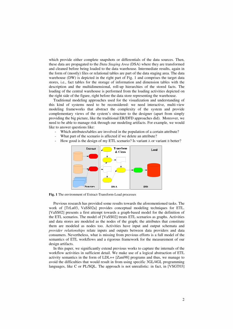
In this paper, we discuss the constructing entities and the usage of blueprints for a particular category of database-centric software, namely, the Extract-Transform-Load (ETL) workflows. ETL workflows are an integral part of the back-stage of data warehouse architectures, where the collection, integration, cleaning and transformation of data takes place, in order to populate the warehouse. In Fig. 1, we abstractly describe the general framework for ETL processes. In the left side, we can observe the original data providers (Sources). Typically, data providers are relational databases and files. The data from these sources are extracted by extraction routines,

2

which provide either complete snapshots or differentials of the data sources. Then, these data are propagated to the Data Staging Area (DSA) where they are transformed and cleaned before being loaded to the data warehouse. Intermediate results, again in the form of (mostly) files or relational tables are part of the data staging area. The data warehouse (DW) is depicted in the right part of Fig. 1 and comprises the target data stores, i.e., fact tables for the storage of information and dimension tables with the description and the multidimensional, roll-up hierarchies of the stored facts. The loading of the central warehouse is performed from the loading activities depicted on the right side of the figure, right before the data store representing the warehouse.

Traditional modeling approaches used for the visualization and understanding of this kind of systems need to be reconsidered: we need interactive, multi-view modeling frameworks that abstract the complexity of the system and provide complementary views of the system’s structure to the designer (apart from simply providing the big picture, like the traditional ER/DFD approaches did). Moreover, we need to be able to manage risk through our modeling artifacts. For example, we would like to answer questions like:

- Which attributes/tables are involved in the population of a certain attribute? - What part of the scenario is affected if we delete an attribute? - How good is the design of my ETL scenario? Is variant A or variant B better?

Sources

Extract Transform

& Clean

DW

Load

DSA

Fig. 1 The environment of Extract-Transform-Load processes

Previous research has provided some results towards the aforementioned tasks. The work of [TrLu03, VaSS02a] provides conceptual modeling techniques for ETL. [VaSS02] presents a first attempt towards a graph-based model for the definition of the ETL scenarios. The model of [VaSS02] treats ETL scenarios as graphs. Activities and data stores are modeled as the nodes of the graph; the attributes that constitute them are modeled as nodes too. Activities have input and output schemata and provider relationships relate inputs and outputs between data providers and data consumers. Nevertheless, what is missing from previous efforts is a full model of the semantics of ETL workflows and a rigorous framework for the measurement of our design artifacts.

In this paper, we significantly extend previous works to capture the internals of the workflow activities in sufficient detail. We make use of a logical abstraction of ETL activity semantics in the form of LDL++ [Zani98] programs and thus, we manage to avoid the difficulties that would result in from using specific 3GL/4GL programming languages, like C or PL/SQL. The approach is not unrealistic: in fact, in [VSGT03]

3

the authors discuss the possibility of providing extensible libraries of ETL tasks, logically described in LDL. On the basis of this result, it is reasonable to assume the reusability of these libraries. Based on this, two particular extensions are given: (a) we treat the cases of insertions/deletions and updates, missing from [VaSS02], and most importantly, (b) we incorporate the internals of the activity semantics to the graph. We provide a principled way of transforming LDL programs to graphs, all the way down to the attribute level. The resulting graph, which is called Architecture Graph can provide sufficient answers to what-if and dependency analysis in the process of understanding or managing the risk of the environment. Moreover, due to the obvious, inherent complexity of this modeling at the finest level of detail, we provide abstraction mechanisms to zoom out the graph at higher levels of abstraction (e.g., visualize the structure of the workflow at the activity level).

The aforementioned contributions deal with the static description of the internals of the ETL workflow and their exploitation during the maintenance or evolution phase. Still, another question can also be answered: “How good is my design?”. The community of software engineering has provided numerable metrics towards evaluating the quality of software designs [Dumk02]. Are these metrics sufficient? In this paper we build upon the fundamental contribution of [BrMB96] that develop a rigorous and systematic framework that classifies usually encountered metrics into five families, each with its own characteristics. These five families are size, length, complexity, cohesion and coupling of software artifacts. In this paper, we develop specific measures for the Architecture Graph and formally prove their fitness for the rigorous framework of [BrMB96].

In a nutshell, our contributions can be listed as follows: − an extension of [VaSS02] to incorporate updates and internal semantics of

activities in the architecture graph; − a principled way of transforming LDL programs to the graph both at the

granular (i.e., attribute) level of detail and at different levels of abstraction; − a systematic definition of software measures for the Architecture Graph, based

on the rigorous framework of [BrMB96]. This paper is organized as follows. In Section 2, we present the graph model for

ETL activities. Section 3 discusses measures for the introduced model. In Section 4, we present related work. Finally, in Section 5 we conclude our results and provide insights for future work.

2. Generic Model of ETL Activities

The purpose of this section is to present a formal logical model for the activities of an ETL environment. Due to the intense data centric nature if ETL workflows, this model abstracts from the technicalities of monitoring, scheduling and logging while it concentrates on the flow of data from the sources towards the data warehouse through the composition of activities and data stores. Initially, we start with the background constructs of the model, already introduced in [VaSS02,VSGT03]. Then, we move on to extend this modeling with formal semantics of the internals of the activities.

4

In order to formally define the semantics of ETL workflow, we can use any 3GL/4GL programming language (C++, PL/SQL etc.). We do not consider the actual implementation of the workflow in some programming language, but rather, we employ LDL++ [Zani98] in order to describe its semantics in a declarative nature and understandable way. LDL++ is a logic-programming, declarative language that supports recursion, complex objects and negation. Moreover, LDL++ supports external functions, choice, (user-defined) aggregation and updates.

LDL was carefully chosen as the language for expressing ETL semantics. First, it is elegant and has a simple model for expressing activity semantics. Second, the head-body combination is particularly suitable for relating both (a) input and output in the simple case, and, (b) consecutive layers of intermediate schemata in complex cases. Finally, LDL is both generic and powerful, so that (large parts of) other languages can be reduced to the Architecture Graph constructs that result from it.

2.1 Preliminaries

In this subsection, we introduce the formal model of data types, data stores and functions, before proceeding to the model of ETL activities. To this end, we reuse the modeling constructs of [VaSS02,VSGT03] upon which we subsequently build our contribution. In brief, the basic components of this modeling framework are:

− Data types. Each data type T is characterized by a name and a domain, i.e., a countable set of values. The values of the domains are also referred to as constants.

− Attributes. Attributes are characterized by their name and data type. For single-valued attributes, the domain of an attribute is a subset of the domain of its data type, whereas for set-valued, their domain is a subset of the powerset of the domain of their data type 2dom(T).

− A Schema is a finite list of attributes. Each entity that is characterized by one or more schemata will be called Structured Entity.

− Records & RecordSets. We define a record as the instantiation of a schema to a list of values belonging to the domains of the respective schema attributes. Formally, a recordset is characterized by its name, its (logical) schema and its (physical) extension (i.e., a finite set of records under the recordset schema). In the rest of this paper, we will mainly deal with the two most popular types of recordsets, namely relational tables and record files.

− Functions. A Function Type comprises a name, a finite list of parameter data types, and a single return data type.

− Elementary Activities. In the [VSGT03] framework, activities are logical abstractions representing parts, or full modules of code. An Elementary Activity (simply referred to as Activity from now on) is formally described by the following elements:

- Name: a unique identifier for the activity. - Input Schemata: a finite list of one or more input schemata that receive

data from the data providers of the activity.

5

- Output Schemata: a finite list of one or more output schemata that describe the placeholders for the rows that pass the checks and transformations performed by the elementary activity.

- Operational Semantics: a program, in LDL++, describing the content passing from the input schemata towards the output schemata. For example, the operational semantics can describe the content that the activity reads from a data provider through an input schema, the operation performed on these rows before they arrive to an output schema and an implicit mapping between the attributes of the input schema(ta) and the respective attributes of the output schema(ta).

- Execution priority. In the context of a scenario, an activity instance must have a priority of execution, determining when the activity will be initiated.

− Provider relationships. These are 1:N relationships that involve attributes with a provider-consumer relationship. The flow of data from the data sources towards the data warehouse is performed through the composition of activities in a larger scenario. In this context, the input for an activity can be either a persistent data store, or another activity. Provider relationships capture the mapping between the attributes of the schemata of the involved entities. Note that a consumer attribute can also be populated by a constant, in certain cases.

− Part_of relationships. These relationships involve attributes and parameters and relate them to their respective activity, recordset or function to which they belong.

Based upon the previous constructs, already available from [VaSS02, VSGT03], we proceed with their extension towards fully incorporating the semantics of ETL workflow in our framework. To this end, we introduce programs as another modeling construct.

− Programs. We assume that the semantics of each activity is given by a declarative program expressed in LDL++. Each program is a finite list of LDL++ rules. Each rule is identified by an (internal) rule identifier. We assume a normal form for the LDL++ rules that we employ. In our setting, there are three types of programs, and normal forms, respectively:

(i) intra-activity programs that characterize the operational semantics, i.e., the internals of activities (e.g., a program that declares that the activity reads data from the input schema, checks for NULL values and populates the output schema only with records having non-NULL values),

(ii) inter-activity programs that link the input/output of an activity to a data provider/consumer,

(iii)side-effect programs that characterize whether the provision of data is an insert, update, or delete action.

We assume that each activity is defined in isolation. In other words, the inter-activity program for each activity is a stand-alone program, assuming the input schemata of the activity as its EDB predicates. Then, activities are plugged in the overall scenario that consists of inter-activity and side-effect rules and an overall scenario program can be obtained from this combination.

6

Intra-activity programs. The intra-activity programs abide by several rules that we list right ahead:

1. All input schemata are EDB predicates. 2. All output schemata appear only as IDB predicates. Furthermore output

schemata are the only IDB predicates that appear in such a program. 3. Intermediate rules are possibly employed to help with intermediate results. 4. We assume non-recursive admissible programs. The safety of the program is

guarantied by the requirement for admissibility, which is a generalization of stratifiability [CeGT90]. An admissible program does not contain any self-referential set definitions or any predicates defined in terms of their own negations.

Inter-activity programs. The inter-activity programs are very simple. There is exactly one rule per provider relationship, with the consumer in the head and the provider in the body. The consumer attributes are mapped to their corresponding providers either through the synonym mechanism or through explicit equalities. No other atoms or predicates are allowed in the body of an inter-activity program; all the consumer attributes should be populated from the provider.

Consumer_input(a1,…,an) <- provider_output(a1,…,am), m ≥ n

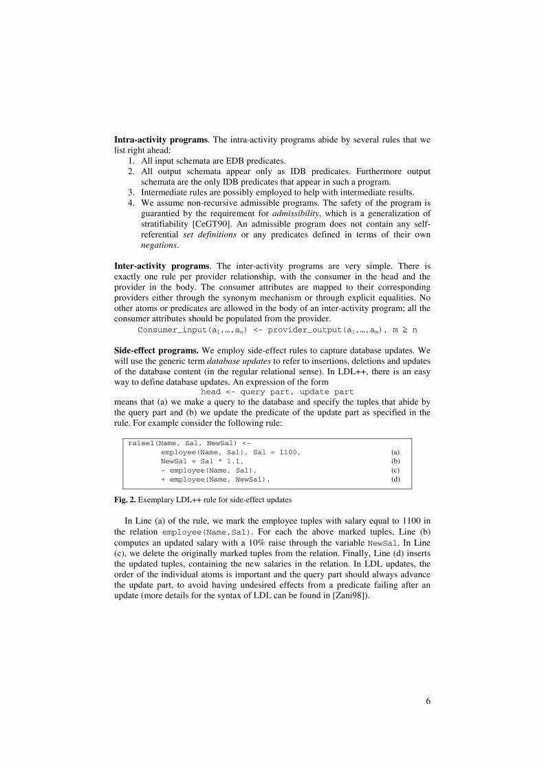
Side-effect programs. We employ side-effect rules to capture database updates. We will use the generic term database updates to refer to insertions, deletions and updates of the database content (in the regular relational sense). In LDL++, there is an easy way to define database updates. An expression of the form

head <- query part, update part means that (a) we make a query to the database and specify the tuples that abide by the query part and (b) we update the predicate of the update part as specified in the rule. For example consider the following rule:

raise1(Name, Sal, NewSal) <- employee(Name, Sal), Sal = 1100, (a) NewSal = Sal * 1.1, (b) - employee(Name, Sal), (c) + employee(Name, NewSal). (d)

Fig. 2. Exemplary LDL++ rule for side-effect updates

In Line (a) of the rule, we mark the employee tuples with salary equal to 1100 in the relation employee(Name,Sal). For each the above marked tuples, Line (b) computes an updated salary with a 10% raise through the variable NewSal. In Line (c), we delete the originally marked tuples from the relation. Finally, Line (d) inserts the updated tuples, containing the new salaries in the relation. In LDL updates, the order of the individual atoms is important and the query part should always advance the update part, to avoid having undesired effects from a predicate failing after an update (more details for the syntax of LDL can be found in [Zani98]).

7

2.2 Incorporating activity semantics in the Architecture Graph

The model of [VSGT03] treats the semantics of activities informally, in terms of its graph model. Each activity is annotated with a tag of its semantics, without these semantics being part of the Architecture Graph. The focus of this work is on the input-output role of the activities instead of their internal operation. In this section, we extend the model of [VSGT03] by translating the formal semantics of the internals of the activities to graph constructs, as part of the overall Architecture Graph. We organize this discussion as follows: first, we consider how individual rules are represented by graphs for all three categories of programs (intra-activity, inter-activity and side-effects). Then, we discuss how the programs of activities are constructed from the composition of different rules and finally, we discuss how a scenario program can be obtained from the composition of the graph representations of inter-activity, intra-activity and side-effect programs.

Intuitively, instead of simply stating which schema populates another schema, we trace how this is done through the internals of an activity. The programs that facilitate the input to output mappings take part in the graph, too. Any filters, joins or aggregations are part of the graph as first-class citizens. Then, there is a straightforward way to determine the architecture graph with respect to the LDL program that defines the ETL scenario. All attributes, activities and relations are nodes of the graph, connected through the proper part-of relationships. Each LDL rule connecting inputs (body of the rule) to outputs (head of the rule) is practically mapped to a set of provider edges, connecting inputs to outputs. Special purpose regulatory edges, capturing filters or joins are also part of the graph.

Intra-activity rules. Given the program of the activity as a stand-alone LDL++ program, we introduce the following constructs, by default:

- A node for the activity per se. - A node for each of the schemata of the activity and a node for the activity

program. Part-of edges connect the activity with these components. - A node for each rule, connected through a part-of relationship to the program

node of the activity. If we treat each rule as a stand-alone program, we can construct its graph as

follows: - We introduce a node for each predicate of the rule. These nodes are connected

to the rule node through a part-of relationship. The edge of the head predicate is tagged as ‘head’ and the edges of the negated literals of the body are tagged as ‘¬’. Functions are treated as predicates. A different predicate node is introduced for each instance of the same predicate (e.g., in the case of a self-join). Such nodes are connected to each other through alias edges. In Subsection 2.3, we detail the tricky parts of the last cases.

- We introduce a node for each variable of a predicate. Part-of relationships connect these nodes with their corresponding predicates.

- For each condition of the form Input attribute = Output attribute (or its equivalent presence of synonyms in the output and input schemata), we add a provider edge. Here, we assume as input (output) attributes, attributes

8

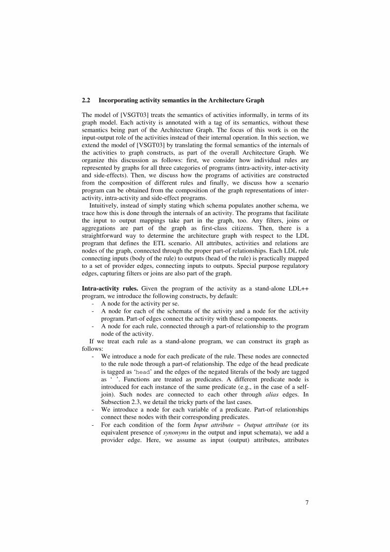
belonging to predicates of the rule body (head). A provider relationship is thus, an edge from the body towards the head of the rule.

- For relationships among input attributes (practically, involving functions and built-ins), a regulator edge is introduced (see next).

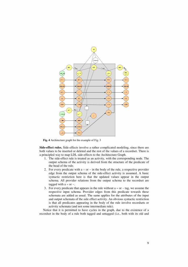
R06: sk.a_in1(pkey,suppkey,date,qty,cost)<- dsa_ps(pkey,suppkey,date,qty,cost). R07: sk.a_in2(pkey,source,skey)<- lookUp(l_pkey,source,l_skey), pkey=l_pkey, skey=l_skey,

source=1. R08: sk.a_out(pkey,suppkey,date,qty,cost,skey)<- add_sk1.a_in1(pkey,date,qty,cost), add_sk1.a_in2(pkey,source,l_skey). R09: dollar2euro.a_in(skey,suppkey,date,qty,cost)<- sk.a_out(pkey,suppkey,date,qty,cost,skey).

Fig. 3 LDL++ for a small part of a scenario

Inter-activity rules. For each recordset of a scenario, we assume a node representing its schema. For simplicity, we do not discriminate a recordset from its schema using different nodes. For each intra-activity rule (between input-output schemata of different activities and/or recordsets) there is a simple way to construct its corresponding graph: we introduce a provider edge from the input towards the output attributes.

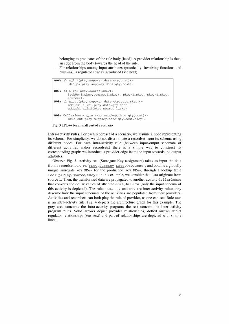
Observe Fig. 3. Activity SK (Surrogate Key assignment) takes as input the data from a recordset DSA_PS(PKey,SuppKey,Date,Qty,Cost), and obtains a globally unique surrogate key SKey for the production key PKey, through a lookup table LookUp(PKey, Source, SKey); in this example, we consider that data originate from source 1. Then, the transformed data are propagated to another activity dollar2euro that converts the dollar values of attribute cost, to Euros (only the input schema of this activity is depicted). The rules R06, R07 and R09 are inter-activity rules: they describe how the input schemata of the activities are populated from their providers. Activities and recordsets can both play the role of provider, as one can see. Rule R08 is an intra-activity rule. Fig. 4 depicts the architecture graph for this example. The grey area concerns the intra-activity program; the rest concern the inter-activity program rules. Solid arrows depict provider relationships, dotted arrows depict regulator relationships (see next) and part-of relationships are depicted with simple lines.

9

pkey

suppkey

date

qty

cost

DSA_PS

R06 head

SK

Program

R08

a_in1 a_outd2e.

a_in

R09

pkey

suppkey

date

qty

cost

l_key

source

l_skey

lookup

R07head

a_in2

pkey

source

skey

=

=

1

headhead

pkey

suppkey

date

skey

cost

skey

suppkey

date

qty

cost

cost

Fig. 4 Architecture graph for the example of Fig. 3

Side-effect rules. Side-effects involve a rather complicated modeling, since there are both values to be inserted or deleted and the rest of the values of a recordset. There is a principled way to map LDL side-effects to the Architecture Graph.

1. The side-effect rule is treated as an activity, with the corresponding node. The output schema of the activity is derived from the structure of the predicate of the head of the rule.

2. For every predicate with a + or – in the body of the rule, a respective provider edge from the output schema of the side-effect activity is assumed. A basic syntactic restriction here is that the updated values appear in the output schema. All provider relations from the output schema to the recordset are tagged with a + or –.

3. For every predicate that appears in the rule without a + or – tag, we assume the respective input schema. Provider edges from this predicate towards these schemata are added as usual. The same applies for the attributes of the input and output schemata of the side effect activity. An obvious syntactic restriction is that all predicates appearing in the body of the rule involve recordsets or activity schemata (and not some intermediate rule).

Notice that it is permitted to have cycles in the graph, due to the existence of a recordset in the body of a rule both tagged and untagged (i.e., both with its old and

10

new values). The old values are mapped to the input schema and the new to the output schema of the side-effect activity.

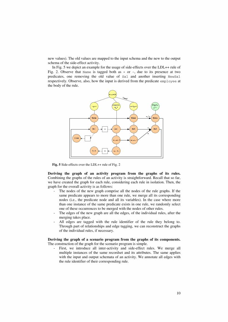
In Fig. 5 we depict an example for the usage of side-effects over the LDL++ rule of Fig. 2. Observe that Name is tagged both as + or –, due to its presence at two predicates, one removing the old value of Sal and another inserting NewSal respectively. Observe, also, how the input is derived from the predicate employee at the body of the rule.

raise1

inputFunctio

n_*output

head

Name

Sal

NewSal

Scale

Name

Sal

NewSal

Sal=

=1.1

=1100

Emplo

yee

Name

Sal

+/-

+

-

Fig. 5 Side-effects over the LDL++ rule of Fig. 2

Deriving the graph of an activity program from the graphs of its rules. Combining the graphs of the rules of an activity is straightforward. Recall that so far, we have created the graph for each rule, considering each rule in isolation. Then, the graph for the overall activity is as follows:

- The nodes of the new graph comprise all the nodes of the rule graphs. If the same predicate appears to more than one rule, we merge all its corresponding nodes (i.e., the predicate node and all its variables). In the case where more than one instance of the same predicate exists in one rule, we randomly select one of these occurrences to be merged with the nodes of other rules.

- The edges of the new graph are all the edges, of the individual rules, after the merging takes place.

- All edges are tagged with the rule identifier of the rule they belong to. Through part of relationships and edge tagging, we can reconstruct the graphs of the individual rules, if necessary.

Deriving the graph of a scenario program from the graphs of its components. The construction of the graph for the scenario program is simple.

- First, we introduce all inter-activity and side-effect rules. We merge all multiple instances of the same recordset and its attributes. The same applies with the input and output schemata of an activity. We annotate all edges with the rule identifier of their corresponding rule.

11

- Then, intra-activity graphs are introduced too. Activity input and output schemata are merged with the nodes that already represent them in the combined intra-activity/side-effect graph. The same applies to activity nodes, too. No other action needs to be taken, since intra-activity programs are connected to the rest of the workflow only through their input and output schemata.

Summarizing, let G(V,E) be the architecture graph of an ETL workflow. Then, the

workflow, apart from schemata, recordsets and activities, has also attributes as its nodes. The edges of the graph are part-of relationships among strong entities and their corresponding components (e.g., activities to schemata, schemata to attributes) and provider relationships among attributes. The internal operation of an activity, provided either by some filtering condition or some function that performs transformations/calculations, is covered through regulator edges (cf. Section 2.3). The direction of provider edges is again from the provider towards the consumer and the direction of the part-of edges is from the container entity towards its components. Edges are tagged appropriately according to their type (part-of or provider).

2.3 Special cases for the modeling of the graph

In this subsection, we extend our basic modeling to cover special cases where particular attention needs to be paid. First, we discuss regulator relationships in detail. Then we discuss aliases, negation, aggregation and functions.

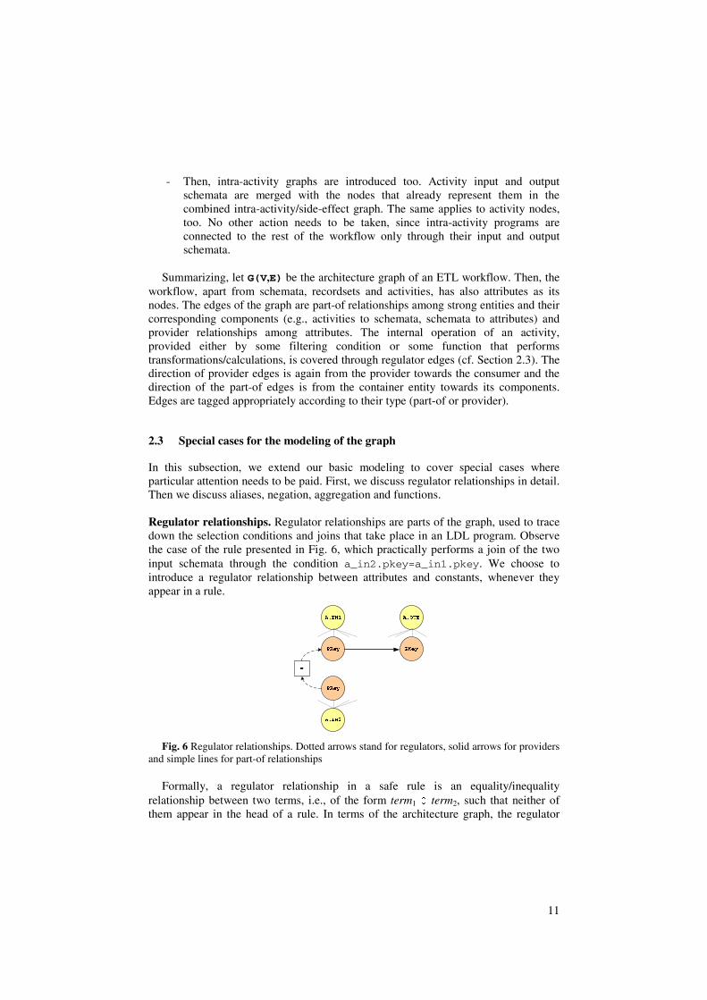
Regulator relationships. Regulator relationships are parts of the graph, used to trace down the selection conditions and joins that take place in an LDL program. Observe the case of the rule presented in Fig. 6, which practically performs a join of the two input schemata through the condition a_in2.pkey=a_in1.pkey. We choose to introduce a regulator relationship between attributes and constants, whenever they appear in a rule.

Fig. 6 Regulator relationships. Dotted arrows stand for regulators, solid arrows for providers and simple lines for part-of relationships

Formally, a regulator relationship in a safe rule is an equality/inequality relationship between two terms, i.e., of the form term1 θ term2, such that neither of them appear in the head of a rule. In terms of the architecture graph, the regulator

12

relationship is represented (a) by a node for each of the terms, (b) by a node representing the condition θ, and (c) by two edges among the node of the condition and the nodes of the term. The direction of the edges follows the way the expression is written in LDL (i.e., from the left to right). For reasons of graphical representation, we will represent condition nodes with squares and regulator relationships with dotted lines.

Notice that there are more than one case that regulator relationships cover: - Input attribute θ constant. In this case, the input attribute is filtered in terms of

a constant. - Input attribute1 θ Input attribute2. In this case, we have a join between input

attributes. Notice that expressions like Input attribute = Output attribute denotes a provider and not a regulator relationship. This is the only case where inputs and outputs are allowed to be linked through equality; this case is covered by provider and not regulator edges. The same applies for the case where the input and the output schema employ the same name for an attribute.

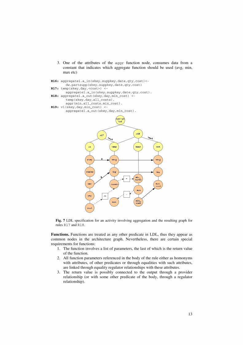
In all the aforementioned cases, θ can take any of the values {=,>,<,≠,≥,≤}, as long as the rule remains safe [CeGT90]. Also, in the above definitions, input attributes may include (a) attributes of the input schemata and (b) attributes of the function schema. Alias relationships. An alias relationship is introduced whenever the same predicate appears in the same rule (e.g., in the case of a self-join). All the nodes representing these occurrences of the same predicate are connected through alias relationships to denote their semantic interrelationship. Note that due to the fact that intra-activity programs do not directly interact with external recordsets or activities, this practically involves the rare case of internal intermediate rules. Negation. When a predicates appears negated in a rule body, then the respective part-of edge between the rule and the literal’s node is tagged with ‘⌐’. Note that negated predicates can appear only in the rule body. Aggregation. Another interesting feature is the possibility of employing aggregation. In LDL, aggregation can be coded in two steps: (a) grouping of values to a bag and (b) application of an aggregate function over the values of the bag. Observe the example of Fig. 7, where data from the table DW.PARTSUPP are summarized, through activity Aggregate1 to provide the minimum daily cost in view V1. In Fig. 7, we list the LDL program for this activity. Rules (R16-R18) explain how the data of table DW.PARTSUPP are aggregated to produce the minimum cost per supplier and day. Observe how LDL models aggregation in rule R17. Then, rule R19 populates view V1 as an inter-activity program.

The graph of an LDL rule is created as usual with only 3 differences: 1. Relations which create a set from the values of a field employ a pair of

regulator edges through an intermediate node‘<>’. 2. Provider relations for attributes used as groupers are tagged with ‘g’.

13

3. One of the attributes of the aggr function node, consumes data from a constant that indicates which aggregate function should be used (avg, min, max etc)

R16: aggregate1.a_in(skey,suppkey,date,qty,cost)<- dw.partsupp(skey,suppkey,date,qty,cost) R17: temp(skey,day,<cost>) <- aggregate1.a_in(skey,suppkey,date,qty,cost). R18: aggregate1.a_out(skey,day,min_cost) <- temp(skey,day,all_costs), aggr(min,all_costs,min_cost). R19: v1(skey,day,min_cost) <- aggregate1.a_out(skey,day,min_cost).

Fig. 7 LDL specification for an activity involving aggregation and the resulting graph for rules R17 and R18.

Functions. Functions are treated as any other predicate in LDL, thus they appear as common nodes in the architecture graph. Nevertheless, there are certain special requirements for functions:

1. The function involves a list of parameters, the last of which is the return value of the function.

2. All function parameters referenced in the body of the rule either as homonyms with attributes, of other predicates or through equalities with such attributes, are linked through equality regulator relationships with these attributes.

3. The return value is possibly connected to the output through a provider relationship (or with some other predicate of the body, through a regulator relationship).

14

For example, observe Fig. 5 where a function involving the multiplication of attribute Sal with a constant is involved. Observe the part-of relationship of the function with its parameters and the regulator relationship with the first parameter and its populating attribute. The return value is linked to the output through a provider relationship.

Moreover, a detailed discussion of the ability to zoom-in/out the Architecture

Graph in different levels of detail (in order to handle the complexity of the graph abstraction) is given in Section 2.4.

2.4 Different levels of detail of the Architecture Graph

As the reader might have guessed, the Architecture Graph is a rather complicated construct, involving the full detail of activities, recordsets, attributes and their interrelationships. Although it is important and necessary to track down this information at design time, in order to formally specify the scenario, it quite clear that this information overload might be cumbersome to manage at later stages of the workflow lifecycle. In other words, we need to provide the user with different versions of the scenario, each at a different level of detail.

We will frequently refer to these abstraction levels of detail simply, as levels. We have already defined the Architecture Graph at the attribute level. The attribute level is the most detailed level of abstraction of our framework. Yet, coarser levels of detail can also be defined. The schema level, abstracts the complexities of attribute interrelationships and presents only how the input and output schemata of activities interplay in the data flow of a scenario. In fact, due to the composite structure of the programs that characterize an activity, there are more than one variants that we can employ for this description. Finally, the coarser level of detail, the activity level, involves only activities and recordsets. In this case, the data flow is described only in terms of these entities.

Architecture Graph at the Schema Level. Let GS(VS,ES) be the architecture graph of an ETL scenario at the schema level. The scenario at the schema level has schemata, functions, recordsets and activities for nodes. The edges of the graph are part-of relationships among structured entities and their corresponding schemata and provider relationships among schemata. The direction of provider edges is again from the provider towards the consumer and the direction of the part-of edges is from the container entity towards its components (in this case just the involved schemata). Edges are tagged appropriately according to their type (part-of or provider).

Intuitively, at the schema level, instead of fully stating which attribute populates another attribute, we trace only how this is performed through the appropriate schemata of the activities. A program, capturing the semantics of the transformations and cleanings that take place in the activity is the means through which the input and output schemata are interconnected. If we wish, instead of including all the schemata of the activity as they are determined by the intermediate rules of the activity’s program, we can present only the program as a single node of the graph, to avoid the extra complexity.

15

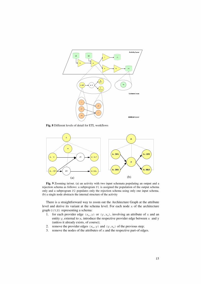
Fig. 8 Different levels of detail for ETL workflows

(a) (b)

Fig. 9 Zooming in/out. (a) an activity with two input schemata populating an output and a rejection schema as follows: a subprogram P1 is assigned the population of the output schema only and a subprogram P2 populates only the rejection schema using only one input schema. (b) a single node abstracts the internal structure of the activity

There is a straightforward way to zoom out the Architecture Graph at the attribute level and derive its variant at the schema level. For each node x of the architecture graph G(V,E) representing a schema:

1. for each provider edge (xa,y) or (y,xa), involving an attribute of x and an entity y, external to x, introduce the respective provider edge between x and y (unless it already exists, of course);

2. remove the provider edges (xa,y) and (y,xa) of the previous step; 3. remove the nodes of the attributes of x and the respective part-of edges.

16

We can iterate this simple algorithm over the different levels of part-of relationships, as depicted in Fig. 9. Architecture Graph at the Activity Level. In this subsection we will deal with the model of ETL scenarios as graphs at the activity level. Only activities and recordsets are part of a scenario at this level. Let GA(VA,EA) be the architecture graph of an ETL scenario at the activity level. The scenario at the activity level has only recordsets and activities for nodes and a set of provider relationships among them for edges. The provider relationships are directed edges from the provider towards the consumer entity.

Intuitively, a scenario is a set of activities, deployed along a graph in an execution sequence that can be linearly serialized. For the moment we do not consider the different alternatives for the ordering of the execution; we simply require that a total order for this execution can be derived (i.e., each activity has a discrete execution priority). Again, we need to stress that we abstract from the complexities of the control flow; the focus of this paper is on the tracing of data flow structure and relationships.

There is a straightforward way to zoom out the Architecture Graph at the schema level and derive its variant at the activity level. For each node x of the architecture graph GA(VA,EA) representing a structured entity (i.e., activity or recordset):

1. for each provider edge (xc,y) or (y,xc), involving a schema of x and an entity y, external to x, introduce the respective provider edge between x and y (unless it already exists, of course);

2. remove the provider edges (xc,y) and (y,xc) of the previous step; 3. remove the nodes of the schema(ta) and program (if x is an activity) of x and

the respective part-of edges.

Discussion. Navigating through different levels of detail is a facility that primarily aims to make the life of the designer and the administrator easier throughout the full range of the lifecycle of the data warehouse. Through this mechanism, the designer can both avoid the complicated nature of parts that are not of interest at the time of the inspection and drill-down to the lowest level of detail for the parts of the design that he is interested in.

Moreover, apart from this simple observation, we can easily show how our graph-based modeling provides the fundamental platform for employing software engineering techniques for the measurement of the quality of the produced design (cf. section 3). Zooming in and out the graph in a principled way allows the evaluation of the overall design both at different depth of granularity and at any desired breadth of range (i.e., by isolating only the parts of the design that are currently of interest).

3. Measuring the Architecture Graph: a principled approach

One of the main roles of blueprints is their usage as testbeds for the evaluation of the design of an engineer. In other words, blueprints serve as the modeling tool that provides answers to the questions “How good is my design?” or “Between these two

17

designs, which one is better?”. In other words, one can define metrics or, more generally, measurement tests, to evaluate the quality of a design. In this section, we will address this issue, for our ETL workflows, in a principled manner.

There is a huge amount of literature devoted in the evaluation of software artifacts. Fenton proves that it is impossible to derive a unique measure of software quality [Fent94]. Rather, measurement theory should be employed in order to define meaningful measures of particular software attributes. A couple of years later, Briand et al., employ measurement theory to provide a set of five generic categories of measures for software artifacts [BrMB96]:

− Size, referring to the number of entities that constitute the software artifact. − Length, referring to the longest path of relationships among these entities. − Complexity, referring to the amount of inter-relationships of a component. − Cohesion, measuring the extent to which each module performs exactly one

job, by evaluating how closely related are its components. − Coupling, capturing the amount of interrelationships between the different

modules of a system. Systems and their modules are considered to be graphs with the nodes representing

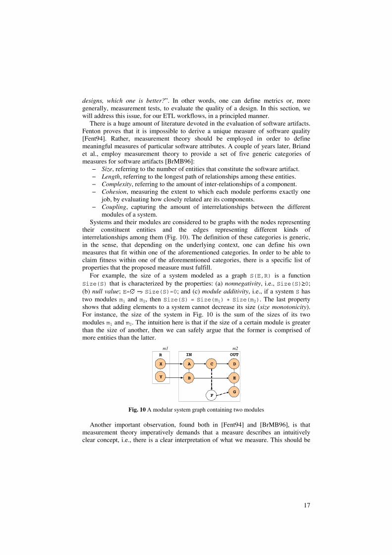
their constituent entities and the edges representing different kinds of interrelationships among them (Fig. 10). The definition of these categories is generic, in the sense, that depending on the underlying context, one can define his own measures that fit within one of the aforementioned categories. In order to be able to claim fitness within one of the aforementioned categories, there is a specific list of properties that the proposed measure must fulfill.

For example, the size of a system modeled as a graph S(E,R) is a function Size(S) that is characterized by the properties: (a) nonnegativity, i.e., Size(S)≥0; (b) null value; E=∅ ⇒ Size(S)=0; and (c) module additivity, i.e., if a system S has two modules m1 and m2, then Size(S) = Size(m1) + Size(m2). The last property shows that adding elements to a system cannot decrease its size (size monotonicity). For instance, the size of the system in Fig. 10 is the sum of the sizes of its two modules m1 and m2. The intuition here is that if the size of a certain module is greater than the size of another, then we can safely argue that the former is comprised of more entities than the latter.

A

B

C D

E

GF

IN OUT

X

Y

R

m1 m2

Fig. 10 A modular system graph containing two modules

Another important observation, found both in [Fent94] and [BrMB96], is that measurement theory imperatively demands that a measure describes an intuitively clear concept, i.e., there is a clear interpretation of what we measure. This should be

18

coupled with clear procedures for determining the parameters of the model and interpreting the results.

In this paper, we propose a set of measures that evaluate our ETL blueprints and

stay within the context of the measures proposed by [BrMB96]. For each measure we provide both its intuition and a proof for its fitness within one of the aforementioned categories. Our fundamental concern, for defining our measures is the effort required (a) to define and (b) to maintain the Architecture Graph, in the presence of changes. Therefore, the statements that one can make, concerning our measures characterize the effort/impact of these two phases of the software lifecycle.

First, we identify the correspondence of the constructs of the Architecture Graph to the concepts of [BrMB96]. [BrMB96] defines a system, S, as a graph S=(E,R), where E is the set of elements of the system and R is the set of relationships between the elements. A module m is a subset of the elements (i.e., the nodes) of the system (observe that a module is defined only in terms of nodes and not edges). In general, modules can overlap. However, when the modules partition the nodes in a system, then this system is called a modular system, MS. The authors distinguish two categories of edges: (a) the intermodule edges that have end points in different modules and (b) the intramodule edges that have end points in the same module. In terms of our modeling:

− The architecture graph G(V,E) is a modular system. − Recordsets and activities are the modules of the graph. The nodes of the graph

involve attributes, functions, constants, etc. All kinds of relationships are the edges of the graph.

− The system is indeed modular, i.e., there are no elements (nodes) that do not belong to exactly one module (activity or recordset). Remember that side-effects are treated as activities.

− Inter-activity and side-effect rules result in intermodule edges. All the rest of the relationships result in intramodule edges.

− The union of two interacting activities can be defined: it requires merging the input/output nodes (attribute/schemata) connected by provider relationships.

3.1 Measures

Next, we define our measures. For each measure, we present: (a) a description; (b) the intuition; and (c) the proof of fitness within the appropriate set of properties of [BrMB96].

Size. Size is a measure of the amount of constituting elements of a system.

Therefore, it can be considered as a reasonable indicator of the amount to define the system. In our framework, we adopt the number of nodes as the measuring rule for the size of the Architecture Graph; thus, the size of the architecture graph G(V,E) is given by the formula:

Size(G) = card(V)

Intuition. Size is an indicator of the effort needed to design an ETL workflow.

19

Proof of Correctness. The function Size satisfies the following properties

[BrMB96]. Property 1: Nonnegativity. The size of a graph G(V,E) is nonnegative, because the

number of its nodes is always non negative (worst case: card(V)=0), i.e., Size(G) = card(V)≥0.

Property 2: Null value. Obviously, the size of a graph G(V,E) is null when if V is empty: V=∅ ⇒ Size(G) = card(V) = 0.

Property 3: Module additivity. The size of a graph G(V,E) is equal to the sum of the sizes of the graphs of two of its modules G1(Vm1,Em1) and G2(Vm2,Em2) such that any element of G is an element of either G1 or G2. Obviously, the number of nodes of the architecture graph is the sum of the number of all its nodes, i.e., recordsets and activities. V = Vm1 ∪ Vm2 ⇒ card(V) = card(Vm1) + card(Vm2) ⇒ Size(G)

= Size(G1) + Size(G2). Length. Length is a measure that refers to the maximum length of

“retransmission” of a certain attribute value. Length measure the longest path that we possibly need to maintain if we make an alteration in the structure of the Architecture Graph. For example, this could involve the deletion of an attribute at the source side. Then, the length characterizes how many nodes in the graph we need to modify as a result of this change (practically involving the nodes corresponding to this particular attribute, within the workflow).

In [VaSS02] the authors define the (transitive) dependency of a node as the cardinality of the (transitive closure of) provider relationships arriving at this node. To define the length of path from a module m backwards to the fountains of the graph, we use the maximum of its transitive dependency measure for the attributes of its output schemata. The only possibility of cycles in the graph of provider relationships is incurred in the case of side-effects. Therefore, we consider a subgraph of the Architecture Graph: for each activity a, if there is a recordset r involved in a cycle with a, due to a side-effect rule, we remove all edges from r towards a. The dependency still holds and no cycles exist in the new graph.

Thereby, the length of a module m is given by the formula:

Length(m)= max{transitive_dependency(i)}, i ∈ output_schemata(m)

The length of the graph is defined as the maximum length over all its modules m:

Length(G)= max(Length(mj))

Observe the reference example of Fig. 3. Although it does not depict a complete graph, the length of the depicted subgraph is 3, since the maximum length of its modules is 3 (input schema of activity $2E).

Intuition. With the measure ‘length’ we determine the maximum path of

reproduction of the same piece of data in the system. Proof of Correctness. Length satisfies the following properties [BrMB96].

20

Property 1: Nonnegativity. The length of a graph G(V,E) is nonnegative, because the minimum path in a graph comprises one node at most. Therefore, Length(G)≥0

Property 2: Null value. An empty graph obviously has a maximum length of 0, therefore, a null value is obtained as the length of the system.

Property 3: Nonincreasing monotonicity for connected components. Consider two nodes of the graph G for which there is a path from one to the other in the nondirected graph obtained from the G by removing directions in the arcs. If a new relationship is introduced between these two nodes, the length of the new graph G’ should not be greater than the length of the original graph G. This is valid in our framework, since we do not allow cycles in the graph. Thus: Length(G)≥Length(G’).

Property 4: Nondecreasing monotonicity for non-connected components. Consider a graph G containing two modules m1 and m2 that are not connected each other. Adding relationships from attributes of m1 to attributes of m2 should not decrease the length of G. This is obvious due to the properties of the max function. Thus, in any addition the length either remains the same or increases.

Property 5: Disjoint Modules. According to this property, the length of a graph G made of two disjoint modules m1 and m2 is equal to the maximum of the lengths of m1 and m2 and clearly, this is inherently covered by the definition of Length(G).

Complexity. Complexity is an inherent property of systems; in our case,

complexity stands to the amount of interconnection of constituent entities of the Architecture Graph. This is an indicator of maintenance effort in the presence of changes. The more complex a system is the more amount of maintenance effort is expected to be required in the case of changes. [BrMB96] indicates that the properties of complexity focus on edges, thus, our function for complexity concerns the edges of the graph G(V,E) at the most detailed level. Again, we distinguish module from system complexity.

We define overall degree of a module to be the overall number of edges of any kind (i.e., provider, part-of, etc) among its components, independently of direction. We count inter-module provider edges as half for each module. Then,

Complexity(m) = |Eintramodule| + 0.5*|Eintermodule|

The complexity of the architecture graph G(V,E) is defined as the summary of the complexities of all the modules of the graph (i.e., recordsets and activities).

Complexity(G) = overall_degree(G)=|E|

Intuition. In our framework, complexity represents the difficulty to maintain a certain combination of activities or the whole ETL scenario.

Proof of Correctness. Complexity satisfies the following properties [BrMB96]. Property 1: Nonnegativity. Obvious, similar to the proof of property 1 for length.

Thus: Complexity(G)≥0. Property 2: Null value. Obvious, since if there is no relationship in the graph, then:

E=∅ ⇒ Complexity(G)=0. Property 3: Symmetry. Complexity should not be sensitive to representation

conventions with respect to the direction of arcs representing system relationships. A

21

relation can be represented in either an “active” (E) or “passive” (E-l) form. The graph and the relationships between its nodes are not affected by these two equivalent representation conventions, and overall degree is insensitive to this by definition. Thus, for graphs G=(V,E) and G-1=(V,E-1) the following formula holds: Complexity(G)= Complexity(G-1).

Property 4: Module monotonicity. This property necessitates that if there exist two modules (i.e., activities or recordsets) that share elements (e.g., attributes) but they do not have any relationship in common, then the complexity of a system is no less than the sum of complexities of the two modules. Considering that two activities or recordsets cannot have a common attribute (element in [BrMB96] terminology), this property trivializes to the next one.

Property 5: Disjoint module additivity. According to this property, the complexity of a graph composed of two disjoint modules is equal to the sum of the complexities of the two modules. This is obvious in our case, since if we consider a graph G of two disjoint activities/recordsets A1 and A2 then the complexity of the graph is the summary of the overall degree of the two activities, since no provider edges exist to relate them and all other kinds of relationships are internal to each module. Thus, the following formula holds: Complexity(G)= Complexity(A1)+ Complexity(A2).

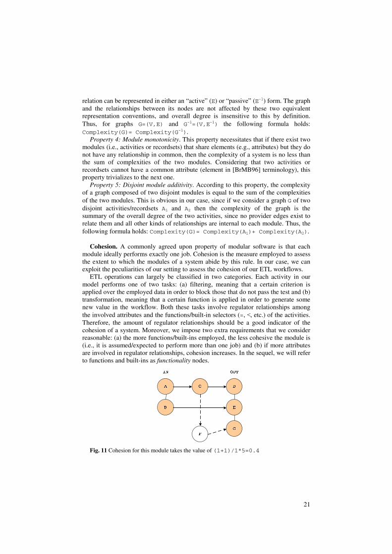
Cohesion. A commonly agreed upon property of modular software is that each

module ideally performs exactly one job. Cohesion is the measure employed to assess the extent to which the modules of a system abide by this rule. In our case, we can exploit the peculiarities of our setting to assess the cohesion of our ETL workflows.

ETL operations can largely be classified in two categories. Each activity in our model performs one of two tasks: (a) filtering, meaning that a certain criterion is applied over the employed data in order to block those that do not pass the test and (b) transformation, meaning that a certain function is applied in order to generate some new value in the workflow. Both these tasks involve regulator relationships among the involved attributes and the functions/built-in selectors (=, ≤, etc.) of the activities. Therefore, the amount of regulator relationships should be a good indicator of the cohesion of a system. Moreover, we impose two extra requirements that we consider reasonable: (a) the more functions/built-ins employed, the less cohesive the module is (i.e., it is assumed/expected to perform more than one job) and (b) if more attributes are involved in regulator relationships, cohesion increases. In the sequel, we will refer to functions and built-ins as functionality nodes.

Fig. 11 Cohesion for this module takes the value of (1+1)/1*5=0.4

22

Before giving the formal definition, we will present the intuition of our proposed measure. Due to requirement (a), we need the inverse of the number of employed functionality nodes. Also due to the requirement (b) we need a measure analog to the number of attributes involved in a regulator relationship. Since [BrMB96] require cohesion to be normalized within a range [0…max] we need to normalize the number of attributes involved with the total number of attributes. To simplify things we measure only input and output attributes. Still, we count an input/output attribute as functionality-related even if it is not directly involved in a regulator relationship, but transitively dependent (or responsible) with an internal attribute that is involved.

In Fig. 11, we depict providers with solid lines and regulators with dotted lines. The input attribute A is involved in a regulator relationship transitively (through attribute C), whereas the attribute G is directly involved in a regulator relationship.

Now, we are ready to define cohesion for our modules and system.

OUT)(IN*F

F_OUTF_IN)Cohesion(m

+

+

= ,

where F is the number of functions of the module, IN (OUT) is the number of input (output) attributes of the module, and F-IN (F-OUT) is the number of functionally-related input (output) attributes of module m.

Cohesion(G) = avg(cohesion(mi)), for all the modules mi of G

Intuition. Cohesion indicates the extent to which (a) a module performs a single task, (b) as many as possibly of its attributes are involved in this task.

Proof of Correctness. The function Cohesion satisfies the following properties

[BrMB96]. Property 1. Nonnegativity and normalization. Obviously module cohesion is a

positive value. The fraction of (F_IN+F_OUT)/(IN+OUT) is obviously lower than 1, therefore cohesion is normalized within [0..1]. Observe that the zero value is obtained if no regulators exist (e.g., the case of an ftp activity) and the maximum value is obtained if all the input and output attributes are involved in the only function employed by the activity. The same apply for the system cohesion.

Property 2. Null Value. Obvious: if no relationships exist, cohesion takes the zero value.

Property 3: Monotonicity. Adding intramodule relationships to a module does not decrease cohesion. There are two cases here: (a) the added relationship is not a regulator (in which case, cohesion remains the same), or (b) the added relationship is a regulator, in which case the cohesion increases. If the cohesion of a module increases, then the average module cohesion increases too.

Property 4: Cohesive modules. Assume we merge two completely unrelated activities. Then, the cohesion of the new module should be lower than the maximum cohesion of the two constituents and the cohesion of the graph G’ obtained by the merger is not greater than the cohesion of the original graph G.

In our case, this can be handled as follows. Replacing two unrelated activities by their union means that we introduce an activity having as input (output) schemata the union of the respective schemata of the two activities. Also, the functionality nodes

23

employed are the same with the ones of the constituents and the same applies for regulator relationships. Assume two activities A1 and A2. Without loss of generality, assume that A1 is more cohesive, therefore:

22

2

11

1

N*F

INV

N*F

INV≥

⇒ INV1*F2*N2≥ INV2*F1*N1

where INVi is the number of functionally-related attributes of activity i and Ni is its total number of input and output attributes. We want to show that:

)2121

21

11

1

N(N*)F(F

INVINV

N*F

INV

++

+≥

This is simple since, if we proceed to the removal of the fractions, we have: INV1*F1*N1+INV1*F1*N2+INV1*F2*N1+INV1*F2*N2 ≥ INV1*F1*N1+ INV2*F1*N1

=> INV1*F1*N2+INV1*F2*N1+INV1*F2*N2 ≥ INV2*F1*N1 which is obvious, since INV1*F2*N2≥ INV2*F1*N1 in the first place.

Therefore, module cohesion does not increase and consequently, the average module cohesion does not increase either.

Coupling. In our framework, coupling captures the amount of relationship between

the attributes belonging to different recordsets or activities (i.e., modules) of the graph. Two kinds of coupling can be defined: inbound coupling and outbound coupling. Given a module m, the former captures the amount of relationships from attributes outside m to attributes inside m; while the latter captures the amount of relationships from attributes inside m to attributes outside m. In what follows, when referring to coupling, we will use the word coupling to denote either inbound or outbound coupling.

[BrMB96] indicates that the properties of complexity focus on intermodule edges, thus our function for complexity concerns the provider edges of the graph G(V,E) that start from an output node of a module and terminate to an input node of another module. Thus, we define the coupling of a graph G(V,E) as the sum of incoming and outgoing provider edges of each activity or recordset. This summary of edges for a certain module is called local degree according to the terminology we introduced in [VaSS02]. Thus, coupling is given by:

Coupling(G) = ∑ilocal_degree(mi), for all the modules mi of G

In the reference example of Section 2, the coupling of the activity SK is 13, i.e., the total number of its incoming and outgoing provider relationships.

Intuition. The coupling of a system denotes the extent to which its different

modules are correlated. Proof of Correctness. Coupling satisfies the following properties [BrMB96]. Property 1: Nonnegativity. Obvious, similar to the proof of property 1 for length.

Thus: Coupling(G)≥0. Property 2: Null value. Obvious, since if there is no relationship in the graph, then:

E=∅ ⇒ Coupling(G)=0.

24

Property 3: Monotonicity. Adding intermodule relationships does not decrease coupling. And this is true, since when a new provider relationship is added the local degree of the respective module is increased, the coupling of this module is increased and the coupling of the whole graph is increased too.

Property 4: Merging of modules. This property is satisfied, because the coupling of a graph G’ obtained by merging two modules is not greater than the coupling of the original graph G, since the two modules may have common intermodule relationships. So, if there is a provider relationship p between the two modules, when these two are merged, then p should be removed from graph and the local degree of the new merged module will be less than the sum of the local degrees of the two modules. Thus, as the property demands, the following is hold: Coupling(G) ≥ Coupling(G’).

Property 5: Disjoint module additivity. According to this property, the coupling of a system obtained by merging two unrelated modules is equal to the coupling of the original system. This is obvious, since if there are not common relationships between the two modules, then the merge of these two does not impose any change to the local responsibilities of their combination. Thus, Coupling(G)=Coupling(G’).

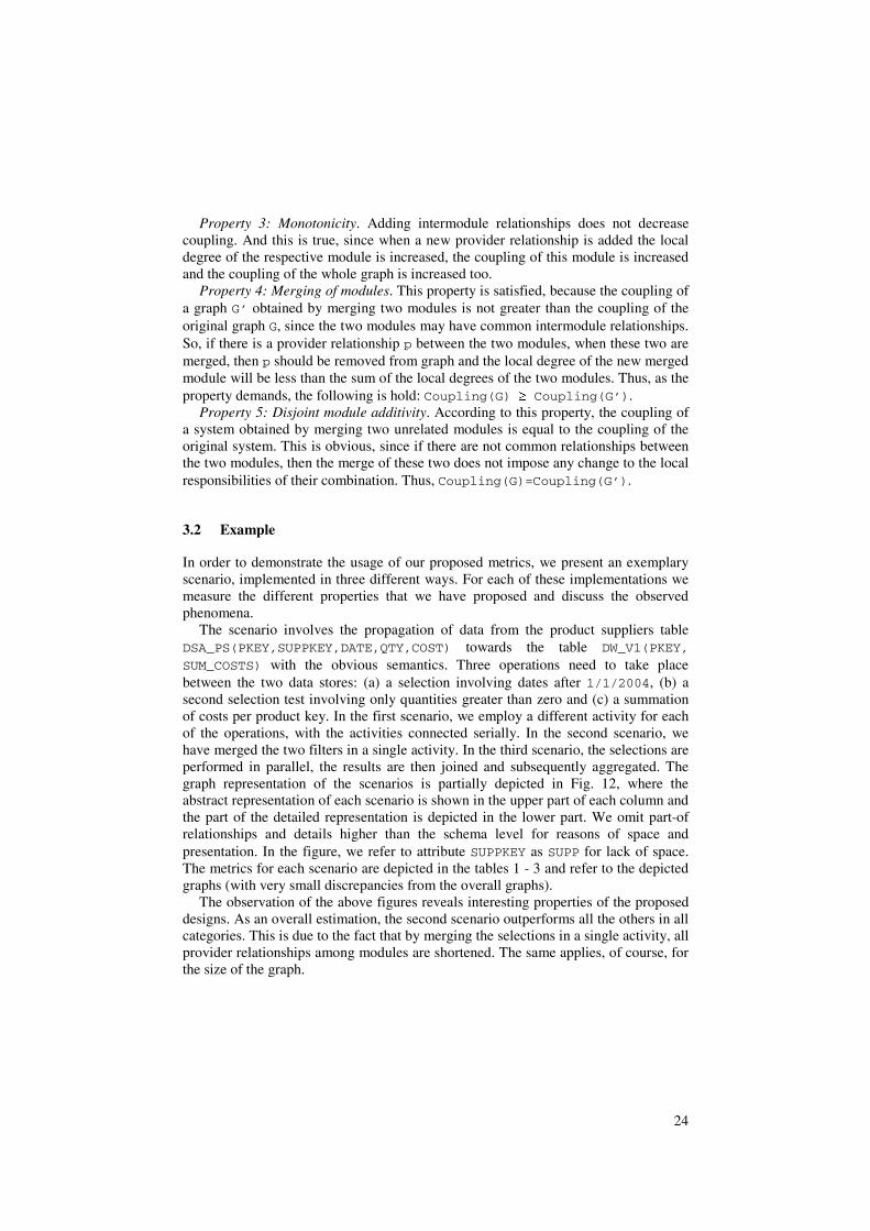
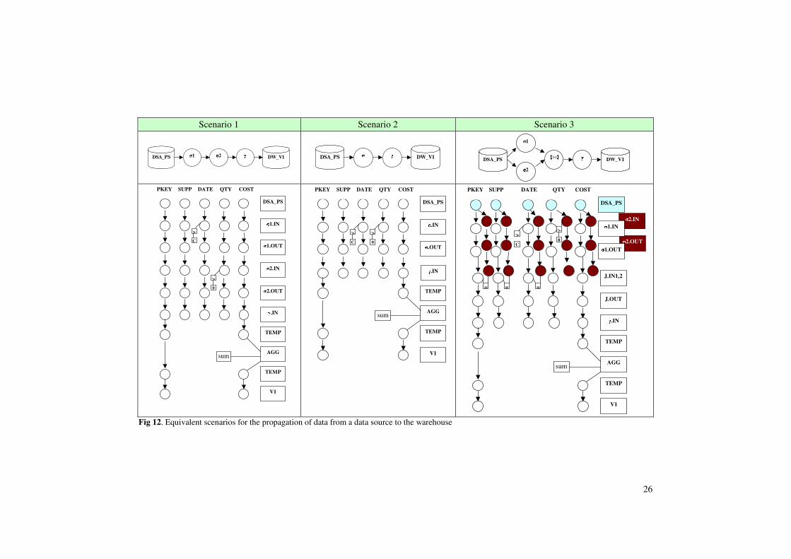
3.2 Example

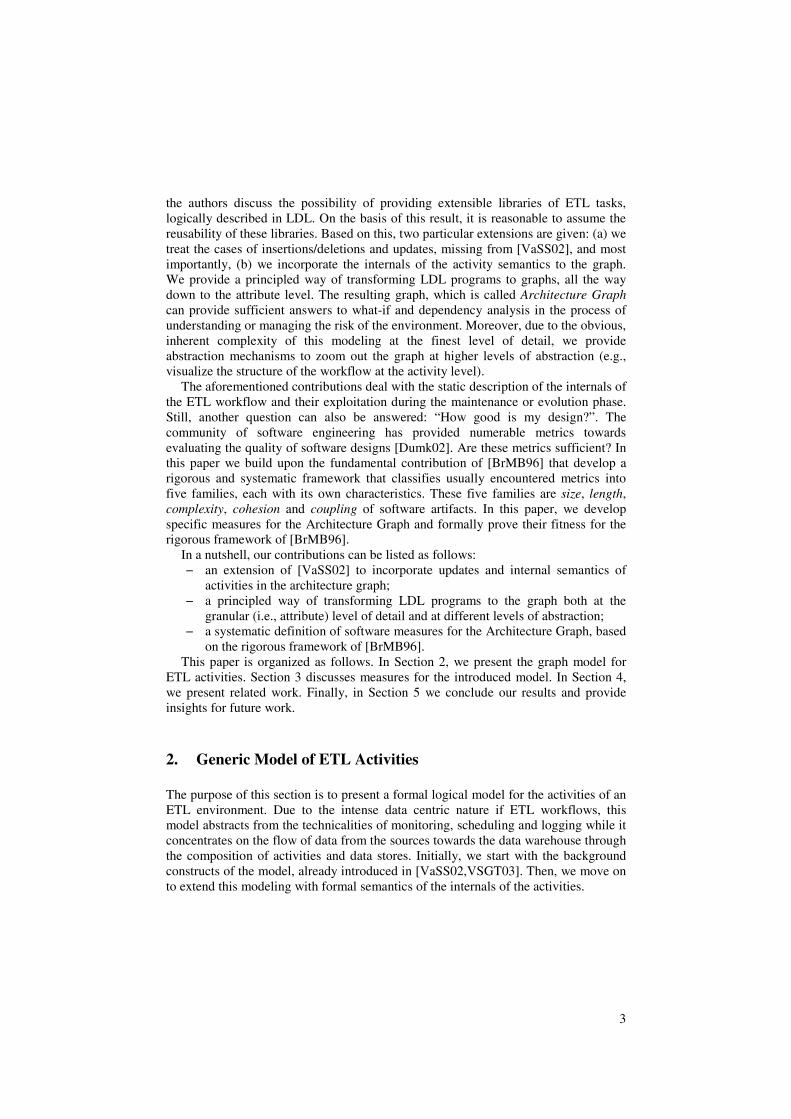
In order to demonstrate the usage of our proposed metrics, we present an exemplary scenario, implemented in three different ways. For each of these implementations we measure the different properties that we have proposed and discuss the observed phenomena.

The scenario involves the propagation of data from the product suppliers table DSA_PS(PKEY,SUPPKEY,DATE,QTY,COST) towards the table DW_V1(PKEY,

SUM_COSTS) with the obvious semantics. Three operations need to take place between the two data stores: (a) a selection involving dates after 1/1/2004, (b) a second selection test involving only quantities greater than zero and (c) a summation of costs per product key. In the first scenario, we employ a different activity for each of the operations, with the activities connected serially. In the second scenario, we have merged the two filters in a single activity. In the third scenario, the selections are performed in parallel, the results are then joined and subsequently aggregated. The graph representation of the scenarios is partially depicted in Fig. 12, where the abstract representation of each scenario is shown in the upper part of each column and the part of the detailed representation is depicted in the lower part. We omit part-of relationships and details higher than the schema level for reasons of space and presentation. In the figure, we refer to attribute SUPPKEY as SUPP for lack of space. The metrics for each scenario are depicted in the tables 1 - 3 and refer to the depicted graphs (with very small discrepancies from the overall graphs).

The observation of the above figures reveals interesting properties of the proposed designs. As an overall estimation, the second scenario outperforms all the others in all categories. This is due to the fact that by merging the selections in a single activity, all provider relationships among modules are shortened. The same applies, of course, for the size of the graph.

25

Table 1: Measures for Scenario 1, involving a linear composition of three activities Size Length Complexity Cohesion Coupling DSA_PS 6 0 7.50 - 5 σ1 14 2 24.00 0.10 10 σ2 14 4 24.00 0.10 10 sum 14 7 20.75 0.29 7 DW_V1 3 8 3.00 - 2 Overall 51 8 79.25 0.16 34

Table 2: Measures for Scenario 2, where selections are merged Size Length Complexity Cohesion Coupling DSA_PS 6 0 7.50 - 5 Σ 16 2 28.00 0.10 10 Sum 14 5 20.75 0.29 7 DW_V1 3 6 3.00 - 2 Overall 39 6 59.25 0.19 24

Table 3: Measures for Scenario 3, where selections are performed in parallel Size Length Complexity Cohesion Coupling DSA_PS 6 0 7.50 - 5 σ1 14 2 24.00 0.10 10 σ2 14 2 24.00 0.10 10 join 20 4 36.50 0.07 15 sum 14 7 20.75 0.29 7 DW_V1 3 8 3.00 - 2 Overall 71 8 115.75 0.14 49

In terms of individual measures, we can observe the following: • Size has obvious results, simply due to the number of attributes in the input

and output schemata of the activities. • The length is a clear indication of the maximum reproduction path of a datum

and, obviously, no major differences are observed. • The complexity and cohesion of the second scenario are quite impressing.

Ideally, for reasons of maintainability, we would appreciate a scenario with low complexity and high cohesion. The complexity of the second scenario is significantly lower than any other alternative, since, obviously, fewer activities and fewer operations are performed. Although the combined selection activity has the same cohesion with the two individual ones (by a simple application of the formula), the overall cohesion drops due to the smaller number of involved activities. Thus, the cohesion of the second scenario is noticeably higher than the other two. Also, the fact that the cohesion of the combined activity remains the same is not surprising: although two selections are performed, the number of attributes involved increases, so the fraction remains stable.

• Finally, the coupling is clearly a subset of the complexity measure: by isolating only provider relationships, we clearly see that module interconnections are lowest when the second scenario is employed.

26

Scenario 1 Scenario 2 Scenario 3

DSA_PS σ1 σ2 γ DW_V1

DSA_PS σ γ DW_V1

DSA_PS

σ1

σ2

γ DW_V1 ��

PKEY SUPP DATE QTY COST

DSA_PS

σ1.IN

σ1.OUT

σ2.IN

σ2.OUT

γ.IN

TEMP

AGG

TEMP

>

C

>

0

sum

V1

PKEY SUPP DATE QTY COST

DSA_PS

σ.IN

σ.OUT

γ.IN

TEMP

AGG

TEMP

>

C

sum

>

0

V1

=

PKEY SUPP DATE QTY COST

DSA_PS

σ2.IN

σ2.OUT

γ.IN

TEMP

AGG

TEMP

>

C

>

0

sum

J.IN1,2

J.OUT

=

σ1.IN

σ1.OUT

=

V1

Fig 12. Equivalent scenarios for the propagation of data from a data source to the warehouse

27

As a final comment, we can easily observe (both by the visualization and

measurement) that there exist attributes that should not participate in the workflow, in the first place. Attribute SUPPKEY (SUPP as a shortcut in Fig. 12) should be omitted in the first place. Attributes DATE and COST should also be omitted once the selections involving them have taken place.

4. Related Work

Two main lines of research pertain to this paper: (a) research on the modeling of ETL activities and (b) research on the measurement of software artifacts and in particular, measurement in a principled way.

As far as ETL is concerned, there is a variety of tools in the market, including the three major database vendors, namely Oracle with Oracle Warehouse Builder [Orac04], Microsoft with Data Transformation Services [Micr04] and IBM with the Data Warehouse Center [IBM04]. Major other vendors in the area are Informatica’s Powercenter [Info04] and Ascential’s DataStage suites [Asce04]. Research-wise, there are several works in the area, including [GFSS00] and [RaHe01] that present systems, tailored for ETL tasks. The main focus of these works is on achieving functionality, rather than on modeling the internals or dealing with the software design or maintenance of these tasks.

Concerning the conceptual modeling of ETL, [TrLu03] and [VaSS02a] are the first attempts that we know of. The former approach employs UML as a modeling language whereas the latter introduces a generic graphical notation. Still, the focus is only on the conceptual modeling part. As far as the logical modeling of ETL is concerned, in [VSGT03] the authors give a template-based mechanism to define ETL workflows. The focus there is on building an extensible library of reusable ETL modules that can be customized to the schemata of the recordsets of each scenario. In an earlier work [VaSS02] the authors have presented a graph-based model for the definition of the ETL scenarios. As already mentioned, we extend this model (a) by treating particular cases like side-effects, but most importantly, (b) by incorporating the internals of the activity semantics to the graph.

Concerning related work on software measurement, we have already mentioned the fundamental works that have guided our approach. [Fent94] gives the fundamentals of measurement theory and the way they should applied in the case of measuring software artifacts. There is an extensive discussion of software metrics in [Dumk02] and an interesting discussion of this area in [FeNe02]. Briand et al. [BrMB96] present the overall framework for defining our particular measures. The particular contribution of this paper is that it gives the principles for defining large categories of software measures. In our case, we prove that the proposed measures fit within the context given by [BrMB96].

28

5. Conclusions

In this paper, we construct the blueprints for the structure ETL workflows by mapping both their inter-connection and their internal semantics to a graph, which we call the Architecture Graph. The Architecture Graph constitutes the blueprint over which we can perform further analysis for the structure of such a workflow. The first of our contributions involves extending existing results in two ways: (a) we explicitly capture the internal semantics of each activity in the workflow, and (b) we incorporate extra information on the interaction of activities with data stores such as the case of updates. We employ the LDL language in order to capture the semantics of ETL activities: therefore, we have provided a principled way of transforming LDL programs to the graph both at the attribute (i.e., granular) level of detail and at different levels of abstraction. Apart from the value that blueprints have per se, we exploit our modeling to introduce rigorous techniques for the measurement of ETL workflows. To this end, we have built upon an existing formal framework for software quality metrics and formally prove how our quality measures fit within this framework.

Research can be continued in more than one direction. We need an extra step, in order to link our results to the control flow of the graph. Precise algorithms for the evaluation of the impact of changes in the Architecture Graph can also be devised. New metrics can also be discovered, if they appear to reveal properties not covered here. Finally, the usage of the Architecture Graph in all phases of the software lifecycle (e.g., testing) can also be evaluated.

References

[Asce04] Ascential Software Inc. Available at: http://www.ascentialsoftware.com [BoRJ99] G. Booch, J. Rumbaugh, I. Jacobson. The Unified Modeling Language User

Guide. Addison-Wesley, 1999 [BrMB96] L.C. Briand, S. Morasca, V.R. Basili. Property-Based Software Engineering

Measurement. In IEEE Trans. on Software Engineering, 22(1), Jan 1996. [BrMB97] L.C. Briand, S. Morasca, V.R. Basili. Comments on “Property-Based Software

Engineering Measurement: Refining the Additivity Properties”. In IEEE Trans. on Software Engineering, 23(3), March 1997.

[CeGT90] S. Ceri, G. Gottlob, L. Tanca. Logic Programming and Databases. Springer-Verlag, 1990.

[Dumk02] R.R. Dumke. Software Metrics: a subdivided bibliography. Available at http://irb.cs.uni-magdeburg.de/sw-eng/us/bibliography/bib_main.shtml

[FeNe02] N.E. Fenton, M. Neil: Software metrics: roadmap. ICSE - Future of SE Track 2000: 357-370.

[Fent94] N. Fenton. Software Measurement: A Necessary Scientific Basis. In IEEE Trans. on Software Engineering, 20(3), March 1994.

[GFSS00] H. Galhardas, D. Florescu, D. Shasha and E. Simon. Ajax: An Extensible Data Cleaning Tool. In Proc. ACM SIGMOD Intl. Conf. On the Management of Data, pp. 590, Dallas, Texas, 2000.

[IBM04] IBM. IBM Data Warehouse Manager. Available at http://www-3.ibm.com/software/data/db2/datawarehouse/

29

[Info04] Informatica. PowerCenter. Available at http://www.informatica.com/products/data+integration/powercenter/default.htm

[Micr04] Microsoft. Data Transformation Services. Available at www.microsoft.com [Orac04] Oracle. Oracle Warehouse Builder Product Page. Available at

http://otn.oracle.com/products/warehouse/content.html [PoDe97] G. Poels, G. Dedene. Comments on “Property-Based Software Engineering

Measurement: Refining the Additivity Properties”. In IEEE Trans. on Software Engineering, 23(3), March 1997.

[RaHe01] V. Raman, J. Hellerstein. Potter's Wheel: An Interactive Data Cleaning System. Proceedings of 27th International Conference on Very Large Data Bases (VLDB), pp. 381-390, Roma, Italy, 2001.

[TrLu03] J. Trujillo, S. Luján-Mora: A UML Based Approach for Modeling ETL Processes in Data Warehouses. In Proc. of the 22nd Intl. Conference on Conceptual Modeling (ER 2003), pp. 307-320, Chicago, IL, USA, October 13-16, 2003

[VaSS02] P. Vassiliadis, A. Simitsis, S. Skiadopoulos. Modeling ETL Activities as Graphs. In Proc. 4th Intl. Workshop on Design and Management of Data Warehouses (DMDW), pp. 52–61, Toronto, Canada, 2002.

[VaSS02a] P. Vassiliadis, A. Simitsis, S. Skiadopoulos. Conceptual Modeling for ETL Processes. In Proc. 5th ACM Intl. Workshop on Data Warehousing and OLAP (DOLAP), pp. 14–21, McLean, Virginia, USA, 2002.

[VSGT03] P. Vassiliadis, A. Simitsis, P. Georgantas, M. Terrovitis. A Framework for the Design of ETL Scenarios. In Proc. 15th Conf. on Advanced Information Systems Engineering (CAiSE '03), pp. 520-535, Klagenfurt/Velden, Austria, June, 2003.

[Zani98] C. Zaniolo. LDL++ Tutorial. UCLA. http://pike.cs.ucla.edu/ldl/, December 1998.