1

Estuarine Environments

Estuaries

!   Estuary is derived from the Latin word for tide - “aestus”

Aestuarium – low ground covered by the sea at high water

!   Estuaries and lagoons comprise 80-90% of coastline along Atlantic & Gulf Coast and 10-20% on Pacific Coast

!   Nearly 900 individual estuaries in the continental US

!   Atlantic & Gulf Coasts - border broad continental shelf - have extensive marshes - older

!   Pacific Coast - formed by tectonic activity, deep, narrow shelf, salt marshes small or absent - younger

The Coastal Zone - Coastal Ocean extends from the high-tide line to the shelf break

This region is responsible for nearly 30% of the total net oceanic primary production and nearly 90% of the global fish catch

2

Definitions of “Estuary” Two major components involved:

•  Transition from fresh (river) water to saline (ocean) water

•  Tidal influence

One definition:

“An estuary is a semi-enclosed coastal water body that extends to the effective limit of tidal influence, within which sea water is significantly diluted with freshwater from land drainage”

Why are features covering such a small portion of the ocean of

importance? •  high primary production

•  fishing, shipping, recreation, aquaculture, etc.

•  most materials entering the ocean from land do so through estuaries

•  population centers

•  most human perturbation of the ocean (pollution, over-exploitation, dredging, etc.) occurs in estuaries

3

From Pinet 2003

Transition zones (ecotones) occur between two or more diverse communities or habitats.

Species that have highest abundance in ecotones are called “edge species”

Odum (1971) - estuaries are ecotones between freshwater and marine habitats

Estuaries can be conceptualized as physical and biological mixing zones

The shallow and intertidal areas are usually bordered by salt marsh or mangrove vegetation (in the tropics)

Estuaries are very efficient “traps” for nutrients, sediments, and pollutants - Usually present in high concentrations

http://www.nmfs.noaa.gov/habitat/habitatprotection/piclink9.htm http://dcm2.enr.state.nc.us/ims/wetlands/salt_marsh.jpg

High socio-economic relevance

4

•  Salt marsh vegetation exists in dynamic equilibrium between rate of sediment accumulation and rate of coastal subsidence, or sea level rise.

-  as deposits accumulate, erosion and OM oxidation increase, slowing rate of further accumulation

-  as sea level rises, marsh is inundated more frequently, and accumulation rate of sediment and peat increases.

- When rate of sedimentation does not kept up with subsidence, marshland is lost.

-  Sea level rise due to global warming could accelerate loss of marshland.

Salt marshes: geomorphology & hydrology

•  Salt marsh soils undergo daily cycle of changing aeration and, thus, redox state.

- high tide: soils are inundated, anaerobic conditions may develop

-  low tide: soils drain, high redox potential re-established in surface layers

•  Tide-induced flushing, combined with groundwater flow from land, leads to large amounts of import(export) from(to) tidal creeks.

-  low tide: low salinity due to flushing of marsh by freshwater runoff from land

-  high tide: marsh is inundated with seawater, highest salinities observed

Salt marshes: geomorphology & hydrology���(cont’d.)

5

Continental Margins

Passive (Atlantic-type) Margins

Atlantic coast and shelf is subsiding because it is a passive margin

The lithospheric plate cools and thickens with age and distance

from the spreading center and sinks (subsides)

Isostatic sinking occurs as sediment accumulates on the shelf

and sediment layer thickens (GOM)

From Pinet 2003

Active (Pacific-type) Margins Tectonic activity occurs along the margin The lithospheric plate is subducted beneath the continental plate Crust is pushed upward to produce an emergent coast Active continental margins usually have narrow shelves.....Passive margins

have wide shelves

From Pinet 2003

6

Shelf Sediments Sediment grain size decreases as you go further offshore due to

wave energy and currents

From Pinet 2003

From Pinet 2003

Shelf Sediments Sediment grain size and feeding strategies

7

Major Factors that Determine Processes on Shelves

Presence or absence of large rivers

Presence or absence of upwelling

Location of ocean boundaries

Shelf width

All of these factors are influenced by climate, hurricanes, El Niño, La Niña, global weather patterns

Based on Geomorphology

Drowned River Valleys or Coastal Plain estuaries (most common)

Formed by sea level rise during the Holocene

tide and river dominated

Examples: Chesapeake Bay, Delaware Bay, Charleston Harbor

From: Pinet 2003

8

Coastal Plain, Bar-Built Estuaries longshore currents form a sand bar or sand spit across an embayment Lack a major river source These estuaries are usually shallow (<2 m) and wind-dominated Example: Galveston Bay , Albemarle-Pamlico Sound

From: Pinet 2003

Fjord-Type Estuaries deep (>100 m), built by glaciers, shallow sill (terminal moraine) sill may trap bottom water that may be anoxic Examples: Puget Sound, coasts of Norway and British Columbia

From: Pinet 2003

9

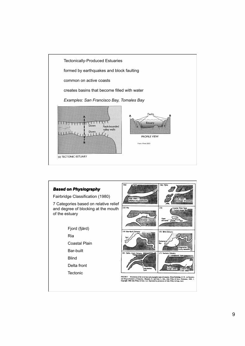
Tectonically-Produced Estuaries formed by earthquakes and block faulting common on active coasts creates basins that become filled with water Examples: San Francisco Bay, Tomales Bay

From: Pinet 2003

Based on Physiography

Fairbridge Classification (1980)

7 Categories based on relative relief and degree of blocking at the mouth of the estuary

Fjord (fjärd)

Ria

Coastal Plain

Bar-built

Blind

Delta front

Tectonic

10

Based on Circulation

and Hydrography Water circulation and stratification influence chemistry and biology

For most estuaries, NET flow is OUT at the surface and IN along the bottom

Two-layered circulation

Longitudinal, lateral, and vertical circulation patterns are

important

Type A - Highly stratified, salt wedge estuary - river discharge dominates over tidal action Salt exchange by vertical advection across the fw/sw interface (halocline). Example: Mississippi River

Estuarine Classification Based on Circulation

From Garrison 2002

From Sverdrup et al 2004

11

Type B - Partially mixed, moderately stratified - tidal flow increases relative to river discharge Vertical advection and turbulence mix the system Example: Chesapeake Bay

Estuarine Classification Based on Circulation

From Garrison 2002

From Sverdrup et al 2004

Type C - Vertically homogeneous and well-mixed Intense tidal flow and strong turbulent mixing, lateral heterogeneity sometimes caused by strong winds e.g., Delaware Bay

Estuarine Classification Based on Circulation

From Sverdrup et al 2004

From Garrison 2002

12

Type D - Fjord - sill results in “stagnant” bottom waters Usually highly-stratified

Estuarine Classification Based on Circulation

From Garrison 2002

From Sverdrup et al 2004

Estuarine Classification Based on Circulation

From: Pinet 2003

13

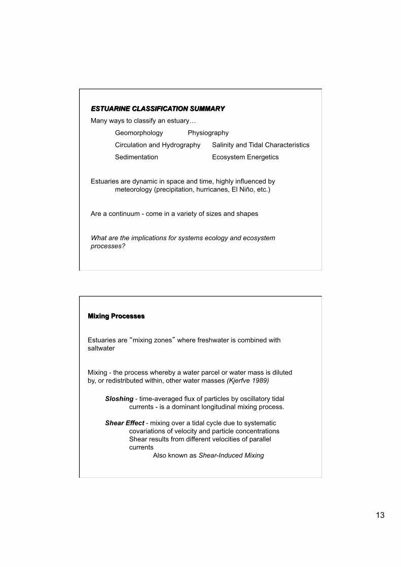
ESTUARINE CLASSIFICATION SUMMARY

Many ways to classify an estuary…

Geomorphology Physiography

Circulation and Hydrography Salinity and Tidal Characteristics

Sedimentation Ecosystem Energetics

Estuaries are dynamic in space and time, highly influenced by meteorology (precipitation, hurricanes, El Niño, etc.)

Are a continuum - come in a variety of sizes and shapes

What are the implications for systems ecology and ecosystem processes?

Mixing Processes

Estuaries are “mixing zones” where freshwater is combined with saltwater

Mixing - the process whereby a water parcel or water mass is diluted by, or redistributed within, other water masses (Kjerfve 1989)

Sloshing - time-averaged flux of particles by oscillatory tidal

currents - is a dominant longitudinal mixing process. Shear Effect - mixing over a tidal cycle due to systematic

covariations of velocity and particle concentrations Shear results from different velocities of parallel currents Also known as Shear-Induced Mixing

14

Advection – the water mass remains intact, but is transported Diffusion - random scattering of water parcels or particles by either random molecular or eddy (turbulent) motions - molecular diffusion usually much less than eddy diffusion

Important at the sediment/water interface

Dispersive Mixing - the scattering of water parcels or particles dissolved in the estuary due to tidal sloshing, shear effects, eddy (turbulent) diffusion, or tidal trapping

Mixing Processes

Estuarine Fronts Boundary between two dissimilar water masses. Commonly form at freshwater/saltwater interface of estuaries and plumes

Surface convergence and advection downward - accumulate particulates at the surface (flotsam & foam lines)

Are different from Langmuir circulation cells - which are driven by friction between wind and water surface

15

rw << sw

rw ≈ sw Nutrients are different!

River-water and Sea-water Concentrations

River-water / Sea-water Ion Ratios

Two major factors:

•  Na+/K+ difference reflects lower affinity of marine rocks for sodium, as compared to potassium (ocean is a less effective sink for sodium)

•  Ca2+/Mg2+ difference reflects preferential removal of calcium in the ocean as biogenic calcite (ocean is a is more effective sink for calcium)

16

Mixing Curve

Assumes end-members are constant over the flushing time of the estuary

Salinity is a conservative constituent in estuaries and is a good indicator of mixing

Constituent plotted against salinity to determine if distribution is attributable to mixing processes (as opposed to non-conservative processes; nutrient uptake, flocculation, biodegradation, etc.)

If concentration vs. salinity is LINEAR, then the chemical/particle exhibits conservative behavior

If plot of concentration vs. salinity is NOT LINEAR, then the chemical/particle exhibits NON-conservative behavior

Non-conservative mixing (source)

Non-conservative mixing (sink)

Mixing Diagram

Examples

(from Day et al. 1989)

17

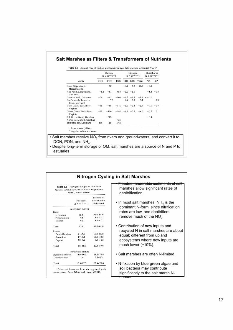
Salt Marshes as Filters & Transformers of Nutrients

• Salt marshes receive NO3 from rivers and groundwaters, and convert it to DON, PON, and NH4.

• Despite long-term storage of OM, salt marshes are a source of N and P to estuaries

Nitrogen Cycling in Salt Marshes • Flooded, anaerobic sediments of salt

marshes allow significant rates of denitrification.

• In most salt marshes, NH4 is the

dominant N-form, since nitrification rates are low, and denitrifiers remove much of the NO3.

• Contribution of new inputs and

recycled N in salt marshes are about equal; different from upland ecosystems where new inputs are much lower (≈10%).

• Salt marshes are often N-limited. • N-fixation by blue-green algae and

soil bacteria may contribute significantly to the salt marsh N-budget.

18

Sulfur Cycling in Salt Marshes • Salt marsh sediments have high SO4-reduction rates, due to high OM, high seawater SO4, and frequent anaerobic conditions.

• Over 50% of the CO2

respired may be due SO4-reduction.

• SO4-reduction produces

H2S, which can then be transformed to pyrite (FeS2) and organic-S.

• Alternatively, H2S can

diffuse upward out of the anaerobic zone and be re-oxidized, so that net < gross SO4-reduction.

Permanent burial of sulfide minerals and dissolved sulfate in marsh sediment.

19

Expected:

Measured:

The Mid-estuary Turbidity Maximum

Turbidity max is due to both 1) chemical flocculation and 2) sediment resuspension

A Mid-estuary Trap for Riverborne Material

Flocculation & resuspension

SEA

20

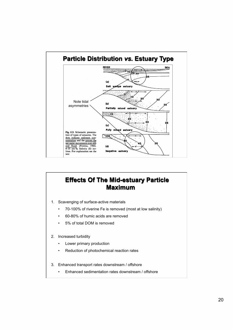
Note tidal asymmetries

Particle Distribution vs. Estuary Type

Effects Of The Mid-estuary Particle Maximum

1.  Scavenging of surface-active materials

•  70-100% of riverine Fe is removed (most at low salinity)

•  60-80% of humic acids are removed

•  5% of total DOM is removed

2.  Increased turbidity

•  Lower primary production

•  Reduction of photochemical reaction rates

3.  Enhanced transport rates downstream / offshore

•  Enhanced sedimentation rates downstream / offshore

21

Water moving down the estuary at velocity u is in geostrophic balance The sides of the estuary counteract the Coriolis force but the water surface is tilted to balance the pressure gradient The Coriolis force balances the pressure gradient In the open ocean, the flow is NOT in geostrophic balance Once the buoyant plume flows out onto the shelf, the surface slope is missing and cannot provide pressure to balance the Coriolis force In the northern hemisphere, the Coriolis force causes the flow to turn to the right and flow along the coast As the Coriolis force pushes water to the right, the blocking coastline causes an opposing pressure gradient in the form of a slight slope in sea level The plume of buoyant water continues as a coastal current in geostrophic balance parallel to the coast

Estuarine Plumes on the Continental Shelf

From: Mann & Lazier 2006

Surface Slope Across an Estuary (the pressure gradient balancing Coriolis)

dh = fuW / g dh = height difference from one side of

the estuary to the other u = flow rate = 0.50 m s-1 W = width of estuary = 200 m f = Coriolis parameter ≈ 10-4 s-1 (at 45º N) g = acceleration due to gravity = 10 m s-2 dh = ((10-4)(0.50)(200))/10 = 0.001 m Thus, the change in height of the water surface across the estuary is 1 mm

Estuarine Plumes on the Continental Shelf

22

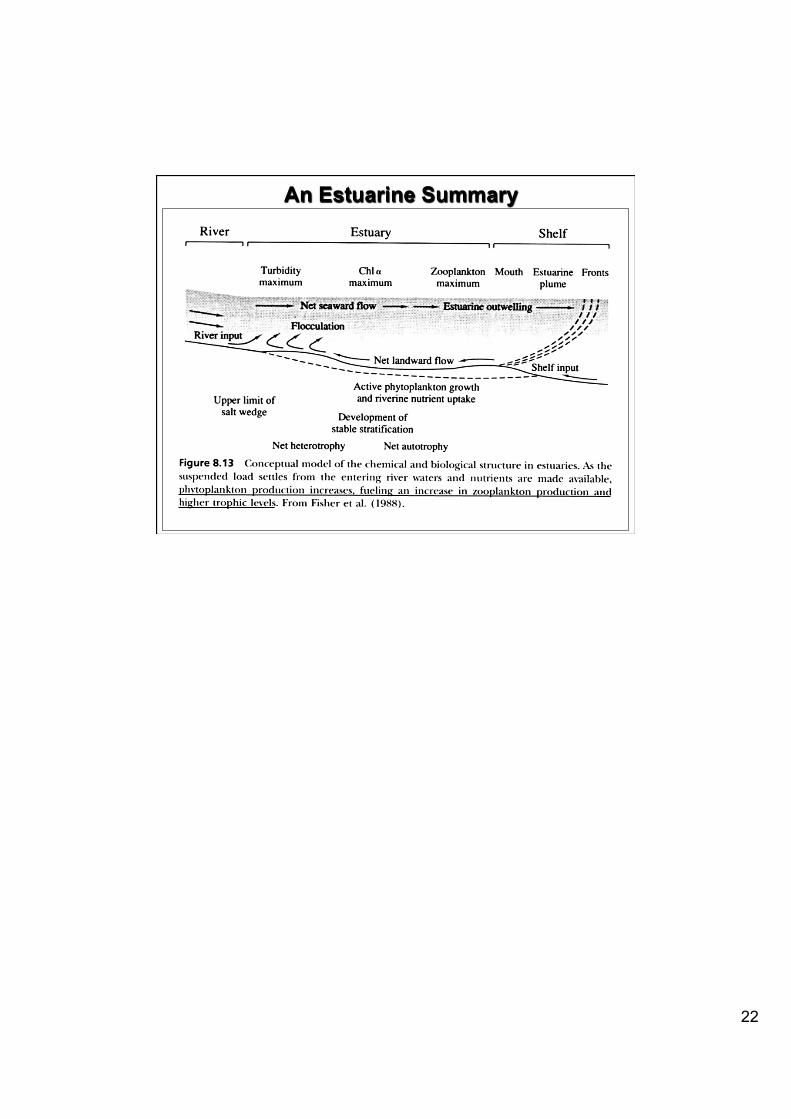
An Estuarine Summary