Estimation of the extreme survival probabilities from ...

HAL Id: hal-00918841https://hal.archives-ouvertes.fr/hal-00918841

Submitted on 15 Dec 2013

HAL is a multi-disciplinary open accessarchive for the deposit and dissemination of sci-entific research documents, whether they are pub-lished or not. The documents may come fromteaching and research institutions in France orabroad, or from public or private research centers.

L’archive ouverte pluridisciplinaire HAL, estdestinée au dépôt et à la diffusion de documentsscientifiques de niveau recherche, publiés ou non,émanant des établissements d’enseignement et derecherche français ou étrangers, des laboratoirespublics ou privés.

Estimation of the extreme survival probabilities fromcensored data

Ion Grama, Jean-Marie Tricot, Jean-François Petiot

To cite this version:Ion Grama, Jean-Marie Tricot, Jean-François Petiot. Estimation of the extreme survival probabili-ties from censored data. BULETINUL ACADEMIEI DE S TIINT E A REPUBLICII MOLDOVA.MATEMATICA, 2014, 74 (1), pp.33-62. �hal-00918841�

https://hal.archives-ouvertes.fr/hal-00918841

https://hal.archives-ouvertes.fr

BULETINUL ACADEMIEI DE STIINTEA REPUBLICII MOLDOVA. MATEMATICANumber 0(0), 1000, Pages 1–27ISSN 1024–7696

Estimation of the extreme survival probabilities

from censored data

Ion Grama, Jean-Marie Tricot and Jean-Francois Petiot

Abstract. The Kaplan-Meier nonparametric estimator has become a standard toolfor estimating a survival time distribution in a right censoring schema. However, ifthe censoring rate is high, this estimator do not provide a reliable estimation of theextreme survival probabilities. In this paper we propose to combine the nonparametricKaplan-Meier estimator and a parametric-based model into one construction. Theidea is to fit the tail of the survival function with a parametric model while for theremaining to use the Kaplan-Meier estimator. A procedure for the automatic choiceof the location of the tail based on a goodness-of-fit test is proposed. This techniqueallows us to improve the estimation of the survival probabilities in the mid and longterm. We perform numerical simulations which confirm the advantage of the proposedmethod.

Mathematics subject classification: 62N01, 62N02, 62G32.Keywords and phrases: Adaptive estimation; Censored data; Model selection; Pre-diction; Survival analysis; Survival probabilities.

1 Introduction

Let (Xi, Ci, Zi)′ , i = 1, ..., n be i.i.d. replicates of the vector (X,C,Z)′ , where

X and C are the survival and right censoring times and Z is a categorical covariate.It is supposed that Xi and Ci are conditionally independent given Zi, i = 1, ..., n.We observe the sample (Ti,∆i, Zi)

′ , i = 1, ..., n, where Ti = min {Xi, Ci} is the ob-servation time and ∆i = 1{Xi≤Ci} is the failure indicator. Let F (x|z) , x ≥ x0 ≥ 0and FC (x|z) , x ≥ x0 be the conditional distributions of X and C, given Z = z,respectively. In this paper we address the problem of estimation of the survivalfunction SF (x|z) = 1− F (x|z) when x ≥ x0 is large. The function SF is tradition-ally estimated using the Kaplan-Meier nonparametric estimator (Kaplan and Meier(1958)). Its properties have been extensively studied by numerous authors, includ-ing Fleming and Harrington (1991), Andersen, Borgan, Gill and Keiding (1993),Kalbfleisch and Prentice (2002), Klein and Moeschberger (2003). However, in vari-ous practical applications, when the time x is close or exceeds the largest observeddata, the predictions based on the Kaplan-Meier and related estimators are ratheruninformative.

For illustration purposes we consider the well known PBC (primary biliary cir-rhosis) data from a clinical trial analyzed in Fleming and Harrington (1991). In thistrial one observes the censored survival times of two groups of patients: the first

c⃝Grama, I., Tricot, J.M. and Petiot, J.F., 2013

1

2 GRAMA, I., TRICOT, J.M. AND PETIOT, J.F.

0 1000 2000 3000 4000 5000 6000 7000

0.0

0.2

0.4

0.6

0.8

1.0

Time (Days)

Sur

viva

l Pro

babi

lity

Kaplan−Meier estimation

DPCA treatmentplacebo

0 1000 2000 3000 4000 5000 6000 7000

0.0

0.2

0.4

0.6

0.8

1.0

Time (Days)

Sur

viva

l Pro

babi

lity

Semiparametric estimation

DPCA treatmentplacebo

Figure 1. We compare two types of prediction of the survival probabilities in DPCA and placebogroups: on the left picture the prediction is based on the Kaplan-Meier estimation and on the rightpicture the prediction uses a semiparametric approach. The points on the curves correspond to thelargest observation time in each group.

one (Z = 1) was given the DPCA (D-penicillamine drug) treatment and the secondone is the control group (Z = 0). The overall censoring rate is about 60%. Here weconsider only the group covariate and we are interested to compare the extreme sur-vival probabilities of the patients under study in the two groups. In Figure 1 (leftpicture) we display the Kaplan-Meier nonparametric curves of the treatment andthe control (placebo) groups. From these curves it seems difficult to infer whetherthe DPCA treatment has an effect on the survival probability. For instance at timex = 4745 (13 years) using the Kaplan-Meier nonparametric estimator (KM), onegets an estimated survival probability SKM (x|z = 0) = 0.3604 for the control groupand SKM (x|z = 1) = 0.3186 for the DPCA treatment group. In this example and inmany other applications one has to face the following two drawbacks. First, the es-timated survival probabilities SKM (x|z) are constant for x beyond the largest (noncensored) survival time, which is not quite helpful for prediction purposes. Second,for this particular data set, the Kaplan-Meier estimation suggests that the DPCAtreatment group has an estimated long term survival probability slightly lower thanthat of the control group, which can be explained by the high variability of SKM (x|z)for large x. These two points clearly rise the problem of correcting the behavior ofthe tail of the Kaplan-Meier estimator.

A largely accepted way to estimate the survival probabilities SF (x|z) for largex, is the parametric-based model fitting the hole data starting from the origin. Itsadvantages are pointed out in Miller (1983), however, it is well known that the biasmodel can be high if it is misspecified. The more flexible nonparametric Kaplan-Meier estimator would generally be preferred for estimating certain functionals ofthe survival curve, as argued in Meier, Karrison, Chappell and Xie (2004). In thispaper we propose to combine the nonparametric Kaplan-Meier estimator and theparametric-based model into one construction which we call semiparametric Kaplan-Meier estimator (SKM). Our new estimator incorporates a threshold t in such away that SF (x|z) is estimated by the Kaplan-Meier estimator for x ≤ t and by aparametric-based estimate for x > t. The main theoretical contribution of the paperis to show that with an appropriate choice of the threshold t such an estimate is

ESTIMATION OF EXTREME SURVIVAL PROBABILITIES 3

0 5 10 15 20 25 30

0.0

0.1

0.2

0.3

0.4

0.5

Time (x)

Roo

t MS

E

MSE(semiparametric)MSE(Kplan−Meier)0.99−quantile

n=20, M=2000, Mean censoring rate=77.5%Root MSE

0 5 10 15 20 25 30

0.0

0.5

1.0

1.5

2.0

Time (x)

Rat

io

Ratio = MSE(semiparametric) / MSE(Kaplan−Meier)0.99−quantile

Ratio of two Root MSE’sn=20, M=2000, Mean censoring rate=77.5%

0 5 10 15 20 25 30

0.0

0.1

0.2

0.3

0.4

0.5

Time (x)

Roo

t MS

E

MSE(semiparametric)MSE(Kplan−Meier)0.99−quantile

n=500, M=2000, Mean censoring rate=77.2%Root MSE

0 5 10 15 20 25 30

0.0

0.5

1.0

1.5

2.0

Time (x)

Rat

io

Ratio = MSE(semiparametric) / MSE(Kaplan−Meier)0.99−quantile

Ratio of two Root MSE’sn=500, M=2000, Mean censoring rate=77.2%

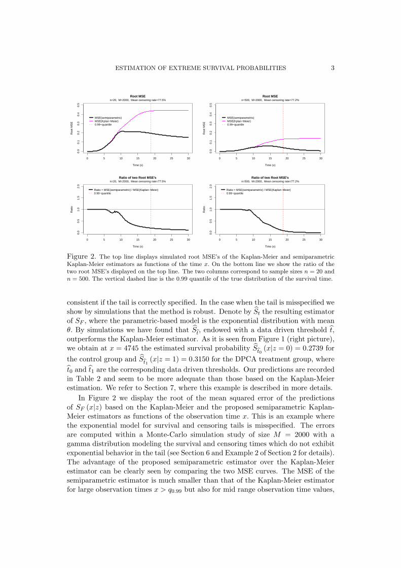
Figure 2. The top line displays simulated root MSE’s of the Kaplan-Meier and semiparametricKaplan-Meier estimators as functions of the time x. On the bottom line we show the ratio of thetwo root MSE’s displayed on the top line. The two columns correspond to sample sizes n = 20 andn = 500. The vertical dashed line is the 0.99 quantile of the true distribution of the survival time.

consistent if the tail is correctly specified. In the case when the tail is misspecified weshow by simulations that the method is robust. Denote by St the resulting estimatorof SF , where the parametric-based model is the exponential distribution with meanθ. By simulations we have found that St, endowed with a data driven threshold t,outperforms the Kaplan-Meier estimator. As it is seen from Figure 1 (right picture),we obtain at x = 4745 the estimated survival probability St0 (x|z = 0) = 0.2739 for

the control group and St1 (x|z = 1) = 0.3150 for the DPCA treatment group, where

t0 and t1 are the corresponding data driven thresholds. Our predictions are recordedin Table 2 and seem to be more adequate than those based on the Kaplan-Meierestimation. We refer to Section 7, where this example is described in more details.

In Figure 2 we display the root of the mean squared error of the predictionsof SF (x|z) based on the Kaplan-Meier and the proposed semiparametric Kaplan-Meier estimators as functions of the observation time x. This is an example wherethe exponential model for survival and censoring tails is misspecified. The errorsare computed within a Monte-Carlo simulation study of size M = 2000 with agamma distribution modeling the survival and censoring times which do not exhibitexponential behavior in the tail (see Section 6 and Example 2 of Section 2 for details).The advantage of the proposed semiparametric estimator over the Kaplan-Meierestimator can be clearly seen by comparing the two MSE curves. The MSE of thesemiparametric estimator is much smaller than that of the Kaplan-Meier estimatorfor large observation times x > q0.99 but also for mid range observation time values,


for example x ∈ [8, q0.99] , where q0.99 is the 0.99-quantile of the distribution F.The proposed extensions of the nonparametric curves are particularly suited forpredicting the survival probabilities in the case when the proportion of the censoredtimes is large. This is the case of the mentioned simulated data where the meancensoring rate is about 77%. Note also that we get an improvement over the Kaplan-Meier estimator even for very low sample sizes like n = 20.

The proposed estimator St is sensible to the choice of the threshold t. The maindifficulty is to choose t small enough, so that the parametric-based part containsenough observation times to ensure a reliable prediction in the tail. At the sametime one should choose t large enough in order to prevent from a large bias due to aninadequate tail fitting. The very important problem of the automatic choice of thethreshold t is treated in Section 5, where a procedure which we call testing-pursuit-selection is performed in two stages: First we test sequentially the null hypothesisthat the proposed parametric-based model fits the data until we detect a chosenalternative. Secondly we select the best model among the accepted ones by penalizedmodel selection. Therefore our testing-pursuit-selection procedure is actually alsoa goodness-of-fit test for the proposed parametric-based model. The resulting datadriven estimator of the tail depends heavily on the testing procedure.

The approach developed here can be applied in conjunction with other techniquesof prediction such as accelerated life testing, see Wei (1992), Tseng, Hsieh andWang (2005), Escobar and Meeker (2006) and extreme values estimation, see Hall(1982), Hall and Welsh (1984, 1985), Dress (1998), Grama and Spokoiny (2008).We refer also to Grama, Tricot and Petiot (2011) for a related result concerning theapproximation of the tail by the Cox model (Cox (1972)).

The case of continuous multivariate covariate Z in the context of a Cox modeland the use of fitted tails other than the exponential can be treated by similarmethods. The models which take into account the cure effects can be reduced toours after removing the cure fraction. However, these problems are beyond the scopeof the paper.

The paper is organized as follows. In Section 2 we introduce the main nota-tions and give the necessary background. The main results of the paper about theconsistency of the proposed estimators are stated in Sections 3 and 4. The auto-matic threshold selection procedure is described in Section 5. In Section 6 we givesome simulation results and analyze the performance of the studied estimators. Anapplication to real data is done in Section 7 and a conclusion in Section 8.

2 The model and background definitions

Assume that the survival and right censoring times arise from variables X andC which take their values in [x0,∞), where x0 ≥ 0. Consider that X and C maydepend on the categorical covariate Z with values in the set Z = {0, ...,m} . Therelated conditional distributions F (x|z) and FC (x|z) , x ≥ x0, given Z = z, aresupposed to belong to the set F of distributions with strictly positive density on[x0,∞). Let fF (·|z) and SF (·|z) = 1−F (·|z) be the conditional density and survival


functions of X, given Z = z. The corresponding conditional hazard function ishF (·|z) = fF (·|z) /SF (·|z) , given Z = z. Similarly, C has the conditional densityfC (·|z) , survival function SC (·|z) and hazard function hC (·|z) = fC (·|z) /SC (·|z) ,given Z = z. We also assume the independence between X and C, conditionallywith respect to Z. Let the observation time and the failure indicator be

T = min {X,C} and ∆ = 1{X≤C},

where 1B is the indicator function taking the value 1 on the event B and 0 otherwise.Let PF,FC

(dx, dδ|z) , x ∈ [x0,∞), δ ∈ {0, 1} be the conditional distribution of thevector Y = (T,∆)′ , given Z = z. The density of PF,FC

is

pF,FC(x, δ|z) = fF (x|z)δ SF (x|z)1−δ fC (x|z)1−δ SC (x|z)δ , (2.1)

where x ∈ [x0,∞), δ ∈ {0, 1} .

Let zi ∈ Z be the observed value of the covariate Zi, where Zi, i = 1, ..., nare i.i.d. copies of Z, and let Yi = (Ti,∆i)

′ , i = 1, ..., n be a sample of n vectors,where each vector Yi has the conditional distribution PF,FC

(·|zi) , given Zi = zi, fori = 1, ..., n. It is clear that, given Z = z ∈ Z, the vectors Yi, i ∈ {j : zj = z} arei.i.d. .

In this paper the problem is to improve the nonparametric Kaplan-Meier esti-mators of the m + 1 survival probabilities SF (x|z) = 1 − F (x|z) , z ∈ Z, for largevalues of x. To this end, we fit the tail of F (·|z) by the exponential distribution withmean θ > 0. Consider the following conditional semiparametric quasi-model

Fθ,t (x|z) =

{F (x|z) , x ∈ [x0, t],

1− (1− F (t|z)) exp(−x−t

θ

), x > t,

(2.2)

where t ≥ x0 is a nuisance parameter and F (·|z) ∈ F , z ∈ Z are functional param-eters. The conditional density, survival and hazard functions of Fθ,t are denoted byfFθ,t

, SFθ,tand hFθ,t

, respectively. Note that hFθ,t(x|z) = 1/θ, for x > t.

The χ2 entropy between two equivalent probability measures P and P0 is definedby χ2 (P, P0) =

∫dP/dP0dP − 1. By Jensen’s inequality χ2 (P, P0) ≥ 0.

Definition 2.1. Let F, FC ∈ F and z ∈ Z. The tail of the distribution F (·|z)belongs to the domain of attraction of the exponential model under the right censoringschema, if there exists a constant θz > 0 such that

limt→∞

χ2(PF,FC

(·|z) , PFθz,t,FC(·|z)

)= 0. (2.3)

Below we give two examples when (2.3) is verified.

Example 1 (asymptotically constant hazards). Consider asymptotically constantsurvival and censoring hazard functions. This model can be related to the familiesof distributions in Hall (1982), Hall and Welsh (1984), Dress (1998) and Grama andSpokoiny (2008) for the extreme value models. Let A > 0, θmax > θmin > 0 be some


constants. Consider that the survival time X has a hazard function hF (·|z) suchthat for some θz ∈ (θmin, θmax) and αz > 0,

|θzhF (θzx|z)− 1| ≤ A exp (−αzx) , x ≥ x0. (2.4)

Condition (2.4) means that hF (x|z) converges to θ−1z exponentially fast as x→ ∞.

Substituting αz = α′zθz, (2.4) gives

∣∣hF (x|z)− θ−1z

∣∣ ≤ A′ exp (−α′zx) , where A

′ =A/θmin.

Similarly, let M > 0, γmax > γmin > 0, µ > 1 be some constants. Assumethat the hazard function hC (·|z) of the censoring time C satisfies for some γz ∈(γmin, γmax) ,

|θzhC (θzx|z)− γz| ≤M (1 + x)−µ , x ≥ x0. (2.5)

Condition (2.5) is equivalent to saying that hC (x|z) approaches γz/θz polynomiallyfast as x → ∞. Substituting γz = γ′zθz, (2.5) gives |hC (x|z)− γ′z| ≤ M ′x−µ, whereM ′ =Mθµmax/θmin.

For example, conditions (2.4) and (2.5) are satisfied if F and FC coincide withthe re-scaled Cauchy distribution Kµ,θ defined below. Let ξ be a variable with thepositive Cauchy distribution K (x) = 2π−1 arctan (x) , x ≥ 0. We define the re-

scaled Cauchy distribution by Kµ,θ (x) = 1 − 1−K(exp((x−µ)/θ))1−K(exp(−µ/θ)) , where µ and θ are

the location and scale parameters. The distribution Kµ,θ can be seen as the excessdistribution of the variable θ log ξ+ µ over the threshold 0. The plots of the densityfKµ,θ

related to Kµ,θ for various values of parameters are given in Figure 4 (topdisplays). We leave to the reader the verification that Kµ,θ fulfills (2.4) with θz = θ,αz = 2 and (2.5) with γz = 1. The distribution Kµ,θ will be used in Section 6 tosimulate survival and censoring times.

Example 2 (non constant hazards). Now we consider the case when the hazardfunctions are not asymptotically constant. For instance, this is the case when thesurvival and censoring times have both gamma distributions. The numerical resultspresented in Figure 2 and discussed in Section 6 show that the approach of the paperworks when conditions (2.4) and (2.5) are not satisfied.

The heuristic argument behind these experimental findings is as follows. Denoteby Q(t) (x) = P (ξ ≤ t+ x|ξ ≥ t) , x ≥ 0, the excess distribution of ξ over the thresh-old t, where ξ is a random variable with distribution Q. Let Gθ be the exponential

distribution with mean θ. Obviously G(t)θ = Gθ. By simple re-normalization, the χ2

entropy in (2.3) can be rewritten as follows:

χ2(PF,FC


)= SF (t|z)SC (t|z)× (2.6)

χ2(PF (t),F

(t)C

(·|z) , PGθz ,F

(t)C

(·|z)).

Clearly from (2.6), the Definition 2.1 is fulfilled if, as t→ ∞,

χ2(PF (t),F

(t)C

(·|z) , PGθz ,F

(t)C

(·|z)) → 0, (2.7)

which means that beyond the threshold t, the excess distribution F (t) (·|z) is ”well”approximated by an exponential distribution with parameter θz, for some t > 0.


However (2.3) can be satisfied even if (2.7) may not hold, more precisely when

χ2(PF (t),F

(t)C

(·|z) , PGθz ,F

(t)C

(·|z)) = o

(1

SF (t|z)

), (2.8)

where SF (t|z) → 0 as t→ ∞. This means that the tail probabilities can be estimatedby our approach even if the exponential model is misspecified for the tail.

3 Consistency of the estimator with fixed threshold

Define the quasi-log-likelihood by Lt (θ|z) =∑n

i=1 log pFθ,t,FC(Ti,∆i|zi) 1{zi=z},

where Fθ,t is defined by (2.2) with parameters θ > 0, t ≥ x0 and F (·|z) ∈ F ,z ∈ Z. Taking into account (2.1) and dropping the terms related to the censoring,the partial quasi-log-likelihood is

Lpartt (θ|z) =

∑

Ti≤t, zi=z

∆i log hFθ,t(Ti|z)−

∑

Ti>t, zi=z

∆i log θ (3.1)

−∑

Ti≤t, zi=z

∫ Ti

x0

hFθ,t(v|z) dv −

∑

Ti>t, zi=z

(∫ t

x0

hFθ,t(v) dv + θ−1 (Ti − t)

),

for fixed z ∈ Z and t ≥ x0.Maximizing Lpartt (θ|z) in θ, obviously yields the estimator

θz,t =

∑Ti>t, zi=z (Ti − t)

nz,t, (3.2)

where by convention 0/0 = ∞ and nz,t =∑

Ti>t, zi=z ∆i is the number of observedsurvival times beyond the threshold t.

The estimator of SF (x) , for x0 ≤ x ≤ t, is easily obtained by standardnonparametric maximum likelihood approach due to Kiefer and Wolfowiz (1956)(see also Bickel, Klaassen, Ritov and Wellner (1993), Section 7.5). We usethe product Kaplan-Meier (KM) estimator (with ties) defined by SKM (x|z) =∏

Ti≤x (1− di (z) /ri (z)) , x ≥ x0, where ri (z) =∑n

j=1 1{Tj≥Ti, zj=z} is the numberof individuals at risk at Ti and di (z) =

∑nj=1 1{Tj=Ti,∆j=1, zj=z} is the number of in-

dividuals died at Ti (see Klein and Moeschberger (2003), Section 4.2 and Kalbfleischand Prentice (2002)). The semiparametric fixed-threshold Kaplan-Meier estimator(SFKM) of the survival function takes the form

St (x|z) =

{SKM (x|z) , x ∈ [x0, t],

SKM (t|z) exp(−x−t

θz,t

), x > t,

(3.3)

where exp(− (x− t) /θz,t

)= 1 if θz,t = ∞. Similarly, it is possible to use the

Nelson-Aalen nonparametric estimator (Nelson 1969, 1972, Aalen, 1976) instead ofthe Kaplan-Meier one.

Consider the Kullback-Leibler divergence K (θ′, θ) =∫log (dGθ′/dGθ) dGθ′ be-

tween two exponential distributions with means θ′ and θ. By convention, K (∞, θ) =


∞. It is easy to see that K (θ′, θ) = ψ (θ′/θ − 1) , with ψ (x) = x−log (x+ 1) , x > −1and that there are two constants c1 and c2 such that (θ′/θ − 1)2 ≤ c1K (θ′, θ) ≤c2 (θ

′/θ − 1)2 , when |θ′/θ − 1| is small enough.The following theorem provides a rate of convergence of the estimator θz,t as

function of the χ2-entropy between PF,FCand PFθ,t,FC

. Let P be the joint distributionof the sample Yi, i = 1, ..., n and E be the expectation with respect to P. In thesequel, the notation αn = OP (βn) means that there is a positive constant c suchthat P (αn > cβn, βn <∞) → 0 as n→ ∞, for any two sequences of positive possiblyinfinite variables αn and βn.

Theorem 3.1. Let z ∈ Z. For any θz > 0 (possibly depending on z) and t ≥ x0, itholds

K(θz,t, θz

)= OP

(n

nz,tχ2(PF,FC


)+

4 log n

nz,t

). (3.4)

For any z ∈ Z and θz > 0 the optimal rate of convergence is obtained when theterms in the right hand side of (3.4) are balanced, i.e. when t = tz,n is chosen suchthat

χ2(PF,FC

(·|z) , PFθz,tz,n ,FC(·|z)

)= O

(log n

n

)as n→ ∞, (3.5)

where tz,n may depend on z. It is easy to verify that, if the tail of the distributionF (·|z) belongs to the domain of attraction of the exponential model under the rightcensoring schema, a sequence tz,n ≥ x0 satisfying (3.5) always exists.

From Theorem 3.1 we deduce the following:

Theorem 3.2. Let z ∈ Z. Assume that the distribution F (·|z) belongs to the domainof attraction of the exponential model under the right censoring schema and tz,n isa sequence satisfying (3.5). Then

K(θz,tz,n , θz

)= OP

(log n

nz,tz,n

). (3.6)

Using the two sided bound for the Kullback-leibler entropy between exponentiallaws stated before, from Theorem 3.2 we conclude that θz,tz,n converges to θz at the

usual(nz,tz,n

)−1/2rate up to a logn factor:

(θz,tz,n − θz

)2= OP

(logn

nz,tz,n

), provided

that there are two constants θmin and θmax such that 0 < θmin ≤ θz ≤ θmax <∞.Furthermore, the rate of convergence of the estimator θz,tz,n can be expressed in

terms of SF (·|z) , SC (·|z) and the sample size n, by giving a lower bound for nz,tz,n .To ensure such a bound we have to introduce two additional assumptions.

The first assumption involves the conditional censoring rate function

qF,FC(t|z) =

∫ ∞

tSF,t (x|z) fC,t (x|z) dx ≤ 1, t ≥ x0, z ∈ Z, (3.7)

where SF,t (x|z) = SF (x|z) /SF (t|z) , x ≥ t is the conditional survival function re-lated to the survival time X, given X > t, and fC,t (x|z) = fC (x|z) /SC (t|z) , x ≥ t


is the conditional density function related to the censoring time C, given C > t. Thequantity qF,FC

(t|z) controls the proportion of the censored times among the obser-vation times exceeding t. In particular if t = x0, then qF,FC

(x0|z) = Prob(X > C|z)is simply the mean censoring rate (given Z = z).

We assume that the conditional censoring rate function qF,FC(·|z) is separated

from 1, i.e. that there are constants r0 ≥ x0 and q0 < 1, such that, for any z ∈ Zand any t ≥ r0,

qF,FC(t|z) ≤ q0. (3.8)

Assumption (3.8) is verified, for instance, if F (·|z) and FC (·|z) are exponential withintensities λX and λC respectively: in this case qF,FC

(t|z) = λC/ (λC + λX) , t ≥ 0.It is also verified if distributions F and FC meet (2.4) and (2.5). The trajectory ofqF,FC

(·|z) with F and FC satisfying the two last conditions is plotted in Figure 4(bottom displays).

The second assumption involves the number of individuals with profile z ∈ Z :nz =

∑ni=1 1 (zi = z) . We assume that there is a constant κ ∈ (0, 1] such that, for

any z ∈ Z,

nz ≥ κn. (3.9)

Lemma 3.3. Assume that conditions (3.8) and (3.9) are satisfied. Then for ev-ery t ≥ r0, it holds Enz,t ≥ κ n (1− q0)SC (t|z)SF (t|z) and P (nz,t < Enz,t/2) ≤exp (−Enz,t/8) . Moreover, if the sequence tz,n is such that Enz,tz,n → ∞ as n→ ∞,then it holds P

(nz,tz,n ≥ Enz,tz,n/2

)→ 1 as n→ ∞.

As a simple consequence of Theorem 3.2 and Lemma 3.3 we have:

Theorem 3.4. Assume conditions (3.8) and (3.9). Assume that the distributionF (·|z) belongs to the domain of attraction of the exponential model under the rightcensoring schema, tz,n is a sequence satisfying (3.5) and

nSC (tz,n|z)SF (tz,n|z) → ∞ as n→ ∞. (3.10)

Then

K(θz,tz,n , θz

)= OP

(log n

nSC (tz,n|z)SF (tz,n|z)

).

4 Explicit computation of the rate of convergence

The results of the previous section show that the rate of convergence of theestimator θz,tz,n depends on the survival functions SF (·|z) and SC (·|z) and on thesequences tz,n. In order to derive a rate of convergence expressed only in terms of thesample size n we have to make additional assumptions on F and FC . Moreover, wefind minimal (up to one term expansion) threshold tz,n for which (3.5) holds true.

Our first result concerns the case when hC (·|z) is separated from 0.


Theorem 4.1. Assume conditions (3.8) and (3.9). Assume that hF (·|z) satisfies(2.4), that there are positive constants tmin and cmin such that hC (x|z) ≥ cmin forany x ≥ tmin and that

SC (tz,n|z)n2αz

1+2αz log1

1+2αz n→ ∞ as n→ ∞. (4.1)

Then,

K(θz,tz,n , θz

)= OP

(n−1 logn

) 2αz1+2αz

SC (tz,n|z)

, (4.2)

where

tz,n =θz

1 + 2αzlog n+ o (log n) .

Assume additionally that SC (tz,n|z) ≥ c0 > 0, which means that with positiveprobability there are large censoring times. Then the rate of convergence in (4.2)

becomes(n−1 log n

) 2αz1+2αz for any z ∈ Z.

Under the additional condition that hC (·|z) satisfies (2.5) we have the followingresult:

Theorem 4.2. Assume condition (3.9). Assume that hF (·|z) satisfies (2.4) andhC (·|z) satisfies (2.5). Then,

K(θz,tz,n , θz

)= OP

((log n

n

) 2αz1+γz+2αz

), (4.3)

where

tz,n =θz

1 + γz + 2αzlog n+ o (log n) .

We give some hints about the optimality of the rate in (4.3). Assume that thesurvival time X is exponential, i.e. hF (x|z) = θ−1

z for all x ≥ x0 and z ∈ Z.This ensures that condition (2.4) is satisfied with any α > 0. Assume conditions(2.5) and (3.9). If there are two constants θmin and θmax such that 0 < θmin ≤

θz ≤ θmax < ∞, (4.3) implies∣∣∣θz,tz,n − θz

∣∣∣ = OP

((n−1 log n

) α1+γz+2α

), for any

α > 0. This rate becomes arbitrarily close to the n−1/2 rate as α → ∞, sincelimα→∞ α/ (1 + γz + 2α) → 1/2. Thus the estimator θz,tz,n almost recovers the usualparametric rate of convergence as α becomes large whatever is γz > 0.

In the case when there are no censoring (γz = 0), after an exponential rescalingour problem can be reduced to that of the estimation of extreme index. If γz → 0

our rate becomes close to n−2αz

1+2αz , which is known to be optimal in the context ofthe extreme value estimation, see Dress (1998) and Grama and Spokoiny (2008). Soour result nearly recovers the best possible rate of convergence in this setting.


5 Testing and automatic selection of the threshold

In this section a procedure of selecting the adaptive estimator θz = θz,tz,n from

the family of fixed threshold estimators θz,t, t ≥ x0 is proposed. Here the adaptivethreshold tz,n is obtained by a sequential testing procedure followed by a selectionusing a penalized maximum likelihood. This motivates our condensed terminologytesting-pursuit-selection used in the sequel. The testing part is actually a multiplegoodness-of-fit testing for the proposed parametric-based models, while the thresholdtz,n can be seen as a data driven substitute for the theoretical threshold tz,n definedin Theorems 4.1 and 4.2 and in the more general Theorems 3.2 and 3.4. For adiscussion on the proposed approach we refer the reader to Section 3 of Grama andSpokoiny (2008). In the sequel, for simplicity of notations, we abbreviate tz = tz,n.

Define a semiparametric change-point distribution by

Fµ,s,θ,t (x|z) =

F (x|z) , x ∈ [x0, s],

1− (1− F (s|z)) exp(−x−s

µ

), x ∈ (s, t],

1− (1− F (s|z)) exp(− t−s

µ

)exp

(−x−t

θ

), x > t,

for µ, θ > 0, x0 ≤ s < t and F (·|z) ∈ F . As in Section 3 we find the maximumquasi-likelihood estimators θz,t of θ and µz,s,t of µ for fixed z ∈ Z and x0 ≤ s < t,which are given by (3.2) and

µz,s,t =nz,sθz,s − nz,tθz,t

nz,s,t,

where nz,s,t =∑

s<Ti≤t, zi=z ∆i and by convention 0 · ∞ = 0 and 0/0 = ∞.Consider a constant D > 0, which will be the critical value in the testing pro-

cedure below. Let k0 ≥ 3 be a starting index and kstep be an increment for k. Letδ′, δ′′ be two positive constants such that 0 < δ′, δ′′ < 0.5. The values k0, kstep, δ

′, δ′′

and D are the parameters of the procedure to be calibrated empirically. Withoutloss of generality, we consider that the Ti’s are arranged in the decreasing order:T1 ≥ ... ≥ Tn. The threshold t will be chosen in the set {T1, ..., Tn} .

The testing-pursuit-selection procedure which we propose is performed in twostages. First we test the null hypothesis HTk

(z) : F = Fθ,Tk(·|z) against the al-

ternative HTk(z) : F = Fµ,Tk,θ,Tl

(·|z) for some δ′k ≤ l ≤ (1− δ′′) k, sequentially

in k = k0 + ikstep, i = 0, ..., [n/kstep], until HTk(z) is rejected. Denote by kz the

obtained break index and define the break time sz = Tkz. Second, using kz and sz

define the adaptive threshold by tz = Tlz

with the adaptive index

lz = argmaxδ′kz≤l≤(1−δ′′)kz

{LTl

(θz,Tl

|z)− LTl

(θz,sz |z

)}, (5.1)

where the term LTl

(θz,sz |z

)is a penalty for getting close to the break time sz. The

resulting adaptive estimator of θz is defined by θz = θz,tz and the semiparamet-


ric adaptive-threshold Kaplan-Meier estimator (SAKM) of the survival function isdefined by Stz (·|z) .

For testing HTk(z) against HTk

(z) we use the statistic

LRmax (Tk|z) = maxδ′k≤l≤(1−δ′′)k

LR (Tk, Tl|z) , (5.2)

where LR (s, t|z) is the quasi-likelihood ratio test statistic for testing Hs (z) : F =Fθ,s (·|z) against the alternative Hs,t (z) : F = Fµ,s,θ,t (·|z) . To compute (5.2), notethat by simple calculations, using (3.1) and (3.2),

Lt

(θz,t|z

)− Lt (θ|z) = nz,tK

(θz,t, θ

), (5.3)

where by convention 0 · ∞ = 0. Similarly to (5.3), the quasi-likelihood ratio teststatistic LR (s, t|z) is given by

LR (s, t|z) = nz,s,tK(µz,s,t, θz,s

)+ nz,tK

(θz,t, θz,s

)(5.4)

with the same convention. Note that, by (5.3), the second term in (5.4) can beviewed as the penalized quasi-log-likelihood

LRpen (s, t|z) = Lt

(θz,t|z

)− Lt

(θz,s|z

)

= nz,tK(θz,t, θz,s

).

Our testing-pursuit-selection procedure reads as follows:Step 1. Set the starting index k = k0.Step 2. Compute the test statistic for testing HTk

(z) against HTk(z) :

LRmax (Tk|z) = maxδ′k≤l≤(1−δ′′)k

LR (Tk, Tl|z)

Step 3. If k ≤ n − kstep and LRmax (Tk|z) ≤ D, increase k by kstep and go to

Step 2. If k > n− kstep or LRmax (Tk|z) > D, let kz = k,

lz = argmaxδ′kz≤l≤(1−δ′′)kz

LRpen

(Tkz, Tl|z

),

take the adaptive threshold as tz = Tlz

and exit.It may happen that with k = k0 it holds LRmax (Tk0 |z) > D, which means

that the hypothesis that the tail is fitted by the exponential model, starting fromTk0 , is rejected. In this case we resume the procedure with a new augmented k0,say with k0 replaced by [ν0k0], where ν0 > 1. Finally, if for each such k0 it holdsLRmax (Tk0 |z) > D, we conclude that the tail of the model cannot be fitted with theproposed parametric tail and we estimate the tail by the Kaplan-Meier estimator.Therefore our testing-pursuit-procedure can be seen as well as a goodness-of-fit testfor the tail.


Note that the Kullback-Leibler entropy K (θ′, θ) is scale invariant, i.e. satisfiesthe identity K (θ′, θ) = K (αθ′, αθ) , for any α > 0 and θ′, θ > 0. Therefore thecritical value D can be determined by Monte Carlo simulations from standard expo-nential observations. The choice of parameters of the proposed selection procedureis discussed in Section 6.

6 Simulation results

We illustrate the performance of the semiparametric estimator (3.3) with fixedand adaptive thresholds in a simulation study. The survival probabilities SF (x|z) ,for large values of x, are of interest.

The mean squared error (MSE) of an estimator S (·|z) of the true survival func-

tion SF (·|z) is defined byMSES(x|z) = E

(S (x|z)− SF (x|z)

)2. The quality of the

estimator S (·|z) with respect to the Kaplan-Meier estimator SKM (·|z) is measuredby the ratio R

S(x|z) =MSE

S(x|z) /MSE

SKM(x|z) .

Without loss of generality, we can assume that the covariate Z takes a fixed valuez. In each study developed below, we perform M = 2000 Monte-Carlo simulations.

We start by giving some hints on the choice of the parameters k0, kstep, δ′, δ′′

of the testing-pursuit-selection procedure in Section 5. The initial value k0 controlsthe variability of the test statistic LRmax (Tk|z) , k ≥ k0. We have fixed k0 as aproportion of the initial sample size: k0 = n/10. The choice kstep = 5 is made tospeed up the computations. The parameters δ′ and δ′′ restrict the high variabilityof the test statistic LR (Tk, Tl|z) when the change point Tl ∈ [Tk, Tk0 ] is close to theends of the interval. The values δ′ = 0.3 and δ′′ = 0.1 are retained experimentally.Our simulations show that the adaptive procedure does not depend much on thechoice of the parameters k0, kstep, δ

′, δ′′.

To choose the critical value D we analyze the type I MSE of the SAKM esti-mator, i.e. the MSE under the null hypothesis that the survival times X1, ..., Xn

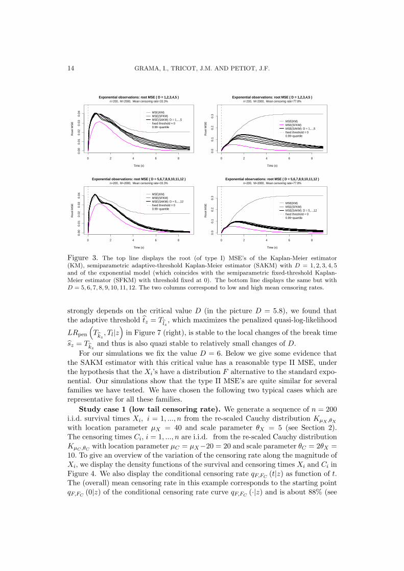
are i.i.d. standard exponential. We perform two simulations using i.i.d. exponentialcensoring times C1, ..., Cn with rates 0.5 and 3.5. The size is fixed at n = 200, butthe results are quite similar for other sizes. The root MSE’s as functions of the timex are given in Figure 3. For comparison, in Figure 3 we also included the MSE’scorresponding to the parametric-based exponential modeling which coincides withthe SFKM estimator having the threshold fixed at 0. Note that the MSE’s calculatedwhen the critical values are D = 1, 2, 3, 4, 5, decrease as D increases (see the topdisplays), while for D = 5, 6, 7, 8, 9, 10, 11, 12 the MSE’s almost do not depend onD (see the top and bottom displays). The simulations show that the type I MSEdecreases as D increases and stabilizes for D ≥ 5. From these plots we conclude thatthe limits for the critical value D can be set between D0 = 5 and D1 = 7 withoutimportant loss in the type I MSE.

It is interesting to note that the adaptive threshold tz is relatively stable tochanges of D. A typical trajectory of the test statistic LRmax (Tk|z) as functionof Tk is drawn in Figure 7 (left). Despite the fact that the break time sz = T

kz


0 2 4 6 8

0.0

00

.01

0.0

20

.03

0.0

4

Time (x)

Ro

ot M

SE

Exponential observations: root MSE ( D = 1,2,3,4,5 )

MSE(KM)MSE(SFKM)MSE(SAKM): D = 1,...,5fixed threshold = 00.99−quantile

n=200, M=2000, Mean censoring rate=33.3%

0 2 4 6 8

0.0

00

.01

0.0

20

.03

0.0

4

Time (x)

Ro

ot M

SE

Exponential observations: root MSE ( D = 5,6,7,8,9,10,11,12 )



0 2 4 6 8

0.0

0.1

0.2

0.3

Time (x)

Ro

ot M

SE

Exponential observations: root MSE ( D = 1,2,3,4,5 )



0 2 4 6 8

0.0

0.1

0.2

0.3

Time (x)

Ro

ot M

SE

Exponential observations: root MSE ( D = 5,6,7,8,9,10,11,12 )



Figure 3. The top line displays the root (of type I) MSE’s of the Kaplan-Meier estimator(KM), semiparametric adaptive-threshold Kaplan-Meier estimator (SAKM) with D = 1, 2, 3, 4, 5and of the exponential model (which coincides with the semiparametric fixed-threshold Kaplan-Meier estimator (SFKM) with threshold fixed at 0). The bottom line displays the same but withD = 5, 6, 7, 8, 9, 10, 11, 12. The two columns correspond to low and high mean censoring rates.

strongly depends on the critical value D (in the picture D = 5.8), we found thatthe adaptive threshold tz = T

lz, which maximizes the penalized quasi-log-likelihood

LRpen

(Tkz, Tl|z

)in Figure 7 (right), is stable to the local changes of the break time

sz = Tkz

and thus is also quazi stable to relatively small changes of D.

For our simulations we fix the value D = 6. Below we give some evidence thatthe SAKM estimator with this critical value has a reasonable type II MSE, underthe hypothesis that the Xi’s have a distribution F alternative to the standard expo-nential. Our simulations show that the type II MSE’s are quite similar for severalfamilies we have tested. We have chosen the following two typical cases which arerepresentative for all these families.

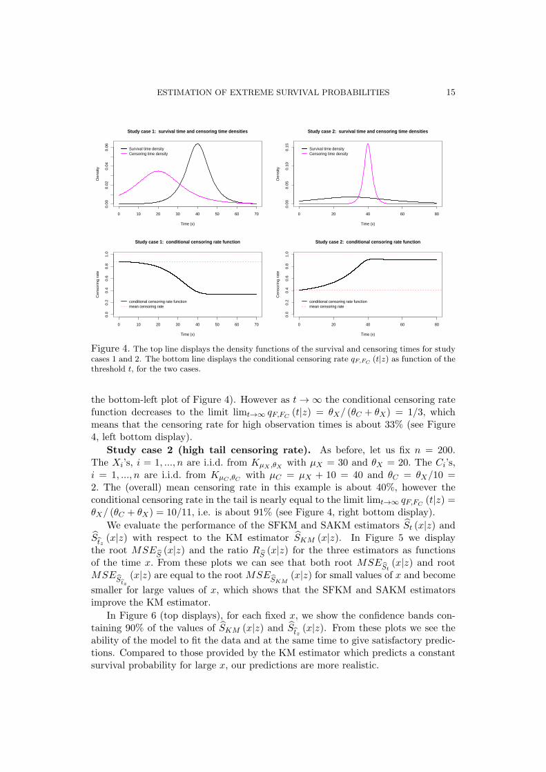
Study case 1 (low tail censoring rate). We generate a sequence of n = 200i.i.d. survival times Xi, i = 1, ..., n from the re-scaled Cauchy distribution KµX ,θX

with location parameter µX = 40 and scale parameter θX = 5 (see Section 2).The censoring times Ci, i = 1, ..., n are i.i.d. from the re-scaled Cauchy distributionKµC ,θC with location parameter µC = µX−20 = 20 and scale parameter θC = 2θX =10. To give an overview of the variation of the censoring rate along the magnitude ofXi, we display the density functions of the survival and censoring times Xi and Ci inFigure 4. We also display the conditional censoring rate qF,FC

(t|z) as function of t.The (overall) mean censoring rate in this example corresponds to the starting pointqF,FC

(0|z) of the conditional censoring rate curve qF,FC(·|z) and is about 88% (see


0 10 20 30 40 50 60 70

0.0

00

.02

0.0

40

.06

Time (x)

De

nsi

ty

Study case 1: survival time and censoring time densities

Survival time densityCensoring time density

0 10 20 30 40 50 60 70

0.0

0.2

0.4

0.6

0.8

1.0

Time (x)

Ce

nso

rin

g r

ate

Study case 1: conditional censoring rate function

conditional censoring rate functionmean censoring rate

0 20 40 60 80

0.0

00

.05

0.1

00

.15

Time (x)

De

nsi

ty

Study case 2: survival time and censoring time densities

Survival time densityCensoring time density

0 20 40 60 80

0.0

0.2

0.4

0.6

0.8

1.0

Time (x)

Ce

nso

rin

g r

ate

Study case 2: conditional censoring rate function

conditional censoring rate functionmean censoring rate

Figure 4. The top line displays the density functions of the survival and censoring times for studycases 1 and 2. The bottom line displays the conditional censoring rate qF,FC

(t|z) as function of thethreshold t, for the two cases.

the bottom-left plot of Figure 4). However as t→ ∞ the conditional censoring ratefunction decreases to the limit limt→∞ qF,FC

(t|z) = θX/ (θC + θX) = 1/3, whichmeans that the censoring rate for high observation times is about 33% (see Figure4, left bottom display).

Study case 2 (high tail censoring rate). As before, let us fix n = 200.The Xi’s, i = 1, ..., n are i.i.d. from KµX ,θX with µX = 30 and θX = 20. The Ci’s,i = 1, ..., n are i.i.d. from KµC ,θC with µC = µX + 10 = 40 and θC = θX/10 =2. The (overall) mean censoring rate in this example is about 40%, however theconditional censoring rate in the tail is nearly equal to the limit limt→∞ qF,FC

(t|z) =θX/ (θC + θX) = 10/11, i.e. is about 91% (see Figure 4, right bottom display).

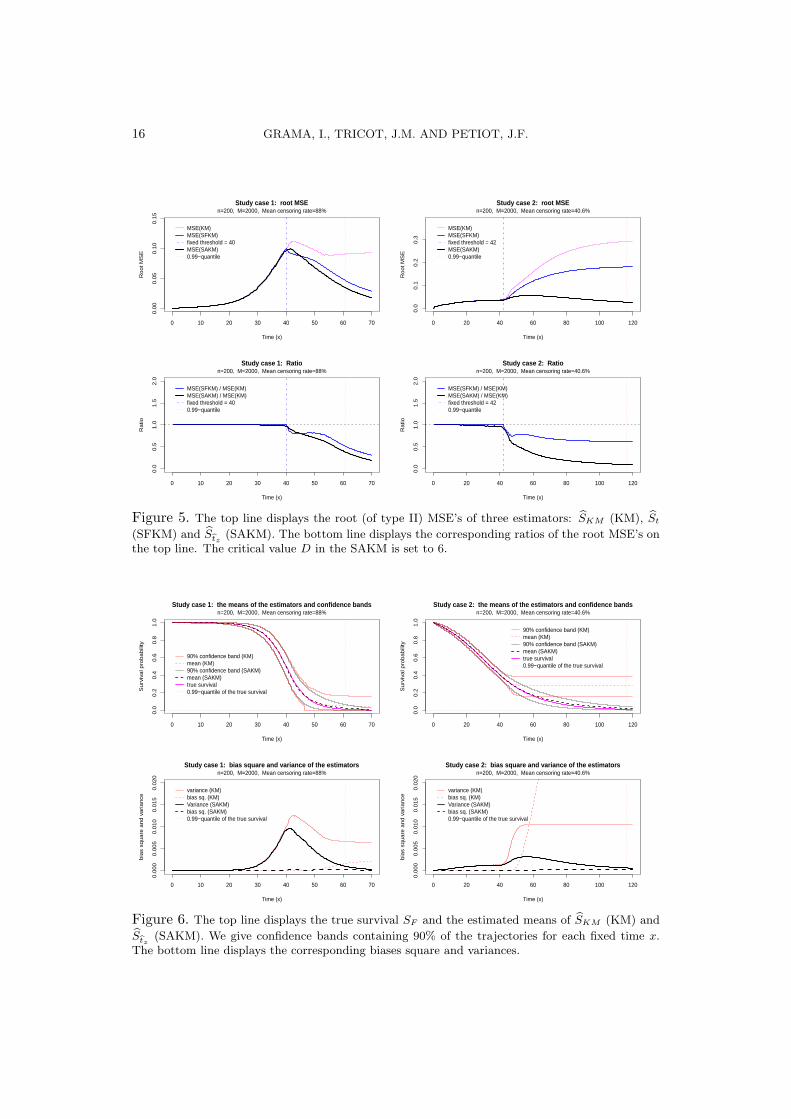
We evaluate the performance of the SFKM and SAKM estimators St (x|z) andStz (x|z) with respect to the KM estimator SKM (x|z). In Figure 5 we displaythe root MSE

S(x|z) and the ratio R

S(x|z) for the three estimators as functions

of the time x. From these plots we can see that both root MSESt(x|z) and root

MSEStz

(x|z) are equal to the rootMSESKM

(x|z) for small values of x and become

smaller for large values of x, which shows that the SFKM and SAKM estimatorsimprove the KM estimator.

In Figure 6 (top displays), for each fixed x, we show the confidence bands con-taining 90% of the values of SKM (x|z) and Stz (x|z). From these plots we see theability of the model to fit the data and at the same time to give satisfactory predic-tions. Compared to those provided by the KM estimator which predicts a constantsurvival probability for large x, our predictions are more realistic.


0 10 20 30 40 50 60 70

0.0

00

.05

0.1

00

.15

Time (x)

Ro

ot

MS

E

Study case 1: root MSEn=200, M=2000, Mean censoring rate=88%

MSE(KM)MSE(SFKM)fixed threshold = 40MSE(SAKM)0.99−quantile

0 10 20 30 40 50 60 70

0.0

0.5

1.0

1.5

2.0

Time (x)

Ra

tio

Study case 1: Ratio

MSE(SFKM) / MSE(KM)MSE(SAKM) / MSE(KM)fixed threshold = 400.99−quantile

n=200, M=2000, Mean censoring rate=88%

0 20 40 60 80 100 120

0.0

0.1

0.2

0.3

Time (x)

Ro

ot

MS

E

Study case 2: root MSEn=200, M=2000, Mean censoring rate=40.6%

MSE(KM)MSE(SFKM)fixed threshold = 42MSE(SAKM)0.99−quantile

0 20 40 60 80 100 120

0.0

0.5

1.0

1.5

2.0

Time (x)

Ra

tio

Study case 2: Ratio

MSE(SFKM) / MSE(KM)MSE(SAKM) / MSE(KM)fixed threshold = 420.99−quantile


Figure 5. The top line displays the root (of type II) MSE’s of three estimators: SKM (KM), St

(SFKM) and Stz(SAKM). The bottom line displays the corresponding ratios of the root MSE’s on

the top line. The critical value D in the SAKM is set to 6.

0 10 20 30 40 50 60 70

0.0

0.2

0.4

0.6

0.8

1.0

Time (x)

Su

rviv

al p

rob

ab

ility

n=200, M=2000, Mean censoring rate=88%Study case 1: the means of the estimators and confidence bands

90% confidence band (KM)mean (KM)90% confidence band (SAKM)mean (SAKM)true survival0.99−quantile of the true survival

0 10 20 30 40 50 60 70

0.0

00

0.0

05

0.0

10

0.0

15

0.0

20

Time (x)

bia

s sq

ua

re a

nd

va

ria

nce

variance (KM)bias sq. (KM)Variance (SAKM)bias sq. (SAKM)0.99−quantile of the true survival

Study case 1: bias square and variance of the estimatorsn=200, M=2000, Mean censoring rate=88%

0 20 40 60 80 100 120

0.0

0.2

0.4

0.6

0.8

1.0

Time (x)

Su

rviv

al p

rob

ab

ility

n=200, M=2000, Mean censoring rate=40.6%Study case 2: the means of the estimators and confidence bands

90% confidence band (KM)mean (KM)90% confidence band (SAKM)mean (SAKM)true survival0.99−quantile of the true survival

0 20 40 60 80 100 120

0.0

00

0.0

05

0.0

10

0.0

15

0.0

20

Time (x)

bia

s sq

ua

re a

nd

va

ria

nce

variance (KM)bias sq. (KM)Variance (SAKM)bias sq. (SAKM)0.99−quantile of the true survival

Study case 2: bias square and variance of the estimatorsn=200, M=2000, Mean censoring rate=40.6%

Figure 6. The top line displays the true survival SF and the estimated means of SKM (KM) and

Stz(SAKM). We give confidence bands containing 90% of the trajectories for each fixed time x.

The bottom line displays the corresponding biases square and variances.


Table 1. Simulations with gamma distributions for survival and censoring times

x 5 6 7 8 9 10 11 12 13SF (x|z) 0.9682 0.9161 0.8305 0.7166 0.5874 0.4579 0.3405 0.2424 0.1658

Mean of Stz

(x|z) 0.9679 0.9159 0.8318 0.7107 0.5686 0.4504 0.3575 0.2853 0.2287

Mean of SKM (x|z) 0.9679 0.9159 0.8306 0.7160 0.5875 0.4581 0.3399 0.2472 0.1888Root MSE

Stz

(x|z) 0.0135 0.0225 0.0336 0.0461 0.0552 0.0606 0.0702 0.0831 0.0940

Root MSESKM

(x|z) 0.0135 0.0225 0.0345 0.0466 0.0604 0.0758 0.0933 0.1144 0.1284

x 14 15 16 17 18 19 20 21 22SF (x|z) 0.1094 0.0699 0.0433 0.0261 0.0154 0.0089 0.0050 0.0028 0.0015

Mean of Stz

(x|z) 0.1841 0.1487 0.1205 0.0979 0.0798 0.0652 0.0534 0.0439 0.0361

Mean of SKM (x|z) 0.1586 0.1453 0.1411 0.1403 0.1402 0.1402 0.1402 0.1402 0.1402Root MSE

Stz

(x|z) 0.0997 0.0998 0.0952 0.0876 0.0785 0.0690 0.0599 0.0515 0.0441

Root MSESKM

(x|z) 0.1384 0.1503 0.1627 0.1731 0.1804 0.1850 0.1877 0.1893 0.1902

0 1000 2000 3000 4000

02

46

8

Time (x)

Test

sta

tistic

Test statistic LRmax

Critical value D = 5.8Tested interval

0 1000 2000 3000 4000

01

23

45

67

Time (x)

Pen

aliz

ed ik

elih

ood

Penalized likelihood LRpen

Tested intervalTesting windowAdaptive threshold

Figure 7. For the placebo group of PBC data we display the test statistics LRmax(Tk|z) as functionof Tk (left) and LRpen(Tk

, Tl|z) as function of Tl (right). The tested interval and the testing windoware given by [T

k, Tk0

] and [T(1−δ′′)k, Tδ′k] respectively. The critical value D is fixed to 5.8.

In Figure 6 (bottom displays) we show the bias square and the variance ofSKM (·|z) and Stz (·|z) . From these plots we see that the variance of Stz (·|z) is

smaller than that of SKM (·|z) in the two study cases. We conclude the same fortheir biases. However, the bias of SKM (·|z) is large in the study case 2 (right bottomdisplay) because of a high conditional censoring rate in the tail (see Figure 4, rightbottom display).

The case of non constant hazards (see Example 2 of Section 2). Theprevious study is performed for models satisfying conditions (2.4) and (2.5). Now weconsider the case when these conditions are not satisfied. Let X and C be generatedfrom gamma distributions whose hazard rate function can be easily verified not to beasymptotically constant (in fact it is slowly varying at infinity). The survival timeX is gamma with shape parameter 10 and rate parameter 1 and the censoring timeC is gamma with shape parameter 8.5 and rate parameter 1.2. The mean censoringrate in this example is about 77%. The results of the simulations are given in Figure2 (n = 20 left picture, n = 500 right picture) and Table 1 (n = 500) for SKM (·|z)and Stz (·|z) . They show that for these distributions the SAKM estimator gives asmaller root MSE than the KM estimator even when the sample size is low (n = 20)and x is in the range of the data.


0 1000 2000 3000 4000 5000 6000 7000

0.0

0.2

0.4

0.6

0.8

1.0

Time (x)

Sur

viva

l pro

babi

lity

DPCA group

SAKMadaptive threshold = 203390%−confidence band

n1=158, M=2000, Censoring rate=41.1%

0 1000 2000 3000 4000 5000 6000 7000

0.0

0.2

0.4

0.6

0.8

1.0

Time (x)

Sur

viva

l pro

babi

lity

Placebo group

SAKMadaptive threshold = 314990%−confidence band

n0=154, M=2000, Censoring rate=39%

Figure 8. For PBC data, we display the pointwise bootstrap 90% confidence intervals for predictedprobabilities. We also display 100 bootstrap trajectories of the predicted probabilities for eachgroup.

Table 2. Predicted survival probabilities for PBC data

x : years 3 4 5 6 7 8 9 10 11x : days 1095 1460 1825 2190 2555 2920 3285 3650 4015DPCA: KM 0.8256 0.7635 0.7077 0.6613 0.5842 0.5417 0.4778 0.4247 0.4247DPCA: SAKM 0.8256 0.7635 0.7077 0.6595 0.5934 0.5340 0.4805 0.4323 0.3890Placebo: KM 0.7911 0.7398 0.7146 0.6950 0.6566 0.6055 0.5461 0.4563 0.3604Placebo: SAKM 0.7911 0.7398 0.7146 0.6950 0.6566 0.6055 0.5497 0.4619 0.3881x : years 12 13 14 15 16 17 18 19 20x : days 4380 4745 5110 5475 5840 6205 6570 6935 7300DPCA: KM 0.3186 0.3186 0.3186 0.3186 0.3186 0.3186 0.3186 0.3186 0.3186DPCA: SAKM 0.3501 0.3150 0.2834 0.2550 0.2295 0.2065 0.1858 0.1672 0.1505Placebo: KM 0.3604 0.3604 0.3604 0.3604 0.3604 0.3604 0.3604 0.3604 0.3604Placebo: SAKM 0.3260 0.2739 0.2302 0.1934 0.1625 0.1365 0.1147 0.0964 0.0810

7 Application to real data

As an illustration we deal with the well known randomized trial in primary biliarycirrhosis (PBC) from Fleming and Harrington (1991) (see Appendix D.1). PBC isa rare but fatal chronic liver disease and the analyzed event is the patient’s death.The trial was open for patient registration between January 1974 and May 1984.The observations lasted until July 1986, when the disease and survival status of thepatients where recorded. There where n = 312 patients registered for the clinicaltrial, including 125 patients who died. The censored times where recorded eitherfor patients which had been lost to follow up or had undergone liver transplantationor was still alive at the study analysis time (July 1986). The number of censoredtimes is 187 and the censoring rate is about 59.9%. The last observed time is 4556which is a censored time. Ties occur for the following three times: 264, 1191 and1690. So there are 122 separate times for which we can observe at least one event.Two treatment groups of patients where compared: the first one (Z = 1) of sizen1 = 158 was given the DPCA (D-penicillamine drug). The second group (Z = 0)of size n0 = 154 was the control (placebo) group. In this example we consider onlythe group covariate. We are interested to predict the survival probabilities of thepatients under study in both groups.

The survival curves based on the KM and SAKM estimators for each group aredisplayed in Figure 1. The numerical results on the predictions appear in Table


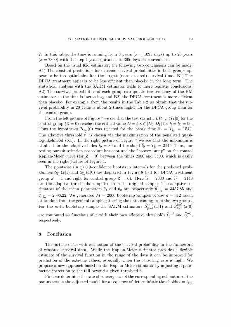
2. In this table, the time is running from 3 years (x = 1095 days) up to 20 years(x = 7300) with the step 1 year equivalent to 365 days for convenience.

Based on the usual KM estimator, the following two conclusions can be made:A1) The constant predictions for extreme survival probabilities in both groups ap-pear to be too optimistic after the largest (non censored) survival time. B1) TheDPCA treatment appears to be less efficient than placebo in the long term. Thestatistical analysis with the SAKM estimator leads to more realistic conclusions:A2) The survival probabilities of each group extrapolate the tendency of the KMestimator as the time is increasing, and B2) the DPCA treatment is more efficientthan placebo. For example, from the results in the Table 2 we obtain that the sur-vival probability in 20 years is about 2 times higher for the DPCA group than forthe control group.

From the left picture of Figure 7 we see that the test statistic LRmax (Tk|0) for thecontrol group (Z = 0) reaches the critical value D = 5.8 ∈ [D0, D1] for k = k0 = 90.Thus the hypotheses Hs0 (0) was rejected for the break time s0 = T

k0= 1542.

The adaptive threshold t0 is chosen via the maximization of the penalized quasi-log-likelihood (5.1). In the right picture of Figure 7 we see that the maximum isattained for the adaptive index l0 = 30 and threshold t0 = T

l0= 3149. Thus, our

testing-pursuit-selection procedure has captured the ”convex bump” on the controlKaplan-Meier curve (for Z = 0) between the times 2000 and 3500, which is easilyseen in the right picture of Figure 1.

The pointwise (in x) 0.9-confidence bootstrap intervals for the predicted prob-abilities St1 (x|1) and St0 (x|0) are displayed in Figure 8 (left for DPCA treatment

group Z = 1 and right for control group Z = 0). Here t1 = 2033 and t0 = 3149are the adaptive thresholds computed from the original sample. The adaptive es-timators of the mean parameters θ1 and θ0 are respectively θ1,t1 = 3457.85 and

θ0,t0 = 2096.22. We generated M = 2000 bootstrap samples of size n = 312 takenat random from the general sample gathering the data coming from the two groups.

For the m-th bootstrap sample the SAKM estimators S(m)

t(m)1

(x|1) and S(m)

t(m)0

(x|0)

are computed as functions of x with their own adaptive thresholds t(m)1 and t

(m)0 ,

respectively.

8 Conclusion

This article deals with estimation of the survival probability in the frameworkof censored survival data. While the Kaplan-Meier estimator provides a flexibleestimate of the survival function in the range of the data it can be improved forprediction of the extreme values, especially when the censoring rate is high. Wepropose a new approach based on the Kaplan-Meier estimator by adjusting a para-metric correction to the tail beyond a given threshold t.

First we determine the rate of convergence of the corresponding estimators of theparameters in the adjusted model for a sequence of deterministic thresholds t = tz,n


for each category z of the model covariate. This is done under the assumption thatthe hazard function is fitted by a constant in the sense that conditions (2.4) and(2.5) are satisfied. It is interesting to note that the rate of convergence depends notonly on the class of survival time distributions but also on the class of censoring timedistributions. By simulations we show that our approach is robust if the (survivaland censoring) fitted tails are misspecified.

In applications the threshold t usually is not known. To overcome this we proposea testing-pursuit-selection procedure which yields an adaptive threshold t = tz,n intwo stages: a sequential hypothesis testing and an adaptive choice of the thresholdbased on the maximization of a penalized quasi-log-likelihood. This testing-pursuit-selection procedure provides also a goodness-of-fit test for the parametric-based partof the model.

We perform numerical simulations with both the fixed and adaptive thresholdestimators. Our simulations show that both estimators improve the Kaplan-Meierestimator not only in the long term, but also in a mid range inside the data. Com-paring the fixed threshold and adaptive threshold estimators, we found that theadaptive choice of the threshold significantly improves on the quality of the predic-tions of the survival function.

We have seen that the quality of estimation of the extreme survival probabilitiesdepends on the conditional censoring rate function, which describes the variationsof the censoring rate as the time increases. The improvement over the Kaplan-Meierestimator is especially effective when the conditional censoring rate is high in thetail.

A Appendix: Proofs of the results

A.1 Auxiliary assertions

The following lemma plays the crucial role in the proof of our main results.Assume that Y1, ...,Yn are i.i.d. with common distribution Q. Let Q be the jointdistribution of Y = (Y1, ...,Yn) . Let Q1, Q0 be two probability measures on R suchthat Q, Q0 and Q1 are equivalent. Define the quasi-log-likelihood ratio by

L (Q1, Q0) =

n∑

i=1

logdQ1

dQ0(Yi) .

Lemma A.1. For any x ≥ 0, n ≥ 1, we have

Q(L (Q1, Q0) > x+ nχ2 (Q,Q0)

)≤ exp

[−x

2

].

Proof. By exponential Chebyshev’s inequality, for any y > 0,

Q (L (Q1, Q0) > y) ≤ exp

[−y/2 + logQ exp

(1

2L (Q1, Q0)

)]. (A.1)


Since Y1, ...,Yn are i.i.d. with common distribution Q, we get

logQ exp

(1

2L (Q1, Q0)

)= n logQ

√dQ1

dQ0. (A.2)

By Holder’s inequality Q(√

dQ1/dQ0

)≤√Q (dQ/dQ0) =

√1 + χ2 (Q,Q0). Using

the last bound and (A.1), (A.2), it follows

Q (L (Q1, Q0) > y) ≤ exp{−y

2+n

2log(1 + χ2 (Q,Q0)

)}

≤ exp{−y

2+n

2χ2 (Q,Q0)

}.

Letting y = x+ nχ2 (Q,Q0) completes the proof.

Now we produce an exponential bound for the quasi-log-likelihood ratio

Lt

(θ′|z)− Lt (θ|z) =

∑

zi=z

logpFθ′,t,FC

pFθ,t,FC

(Yi|z) .

Lemma A.2. For any θ, θ′ ∈ R, z ∈ Z and any x ≥ 0 it holds

P(Lt

(θ′|z)− Lt (θ|z) > x+ nχ2

(PF,FC

(·|z) , PFθ,t,FC(·|z)

))≤ exp

(−x

2

).

Proof. Let Iz = {i : zi = z} . Note that Yi = (Ti,∆i)′ , i ∈ Iz, are i.i.d. variables. We

apply Lemma A.1 with Y = {Yi : i ∈ Iz} and Q = PF,FC(·|z) , Q0 = PFθ,t,FC

(·|z) ,Q1 = PFθ′,t,FC

(·|z) , which ends the proof.

Next, we give an exponential bound for the maximum quasi-log-likelihood ratiowhich permits to obtain a rate of convergence of θz,t.

Lemma A.3. For any θ > 0, t ≥ x0 and any x ≥ 0 it holds

P

(nz,tK

(θz,t, θ

)> x+ nχ2

(PF,FC

(·|z) , PFθ,t,FC(·|z)

)+ 2 logn

)≤ 2 exp

(−x

2

),

where z ∈ Z and by convention 0 · ∞ = 0.

Proof. We prove that

P

(nz,tK

(θz,t, θ

)> y)≤ 2n exp (−x/2) = 2 exp (−x/2 + log n) , (A.3)

where y = x+ nχ2(PF,FC

(·|z) , PFθ,t,FC(·|z)

)≥ 0.

Since nz,tθz,t =∑

Ti>t, zi=z (Ti − t) , by direct calculations, we have Lt (θ′|z) −

Lt (θ|z) = nz,tΛz (θ′) , where Λz (u) = log (θ/u) −

(u−1 − θ−1

)θz,t. Using that

K (θ′, θ) = θ′/θ − 1 − log (θ′/θ) , we deduce K(θz,t, θ

)= Λz

(θz,t

). Denote for

brevity g (u, k) = (log (θ/u)− y/k) /(u−1 − θ−1

), u = θ. Note that, for 0 < u < θ


the inequality kΛz (u) > y is equivalent to g (u, k) > θz,t and for u > θ the inequal-

ity kΛz (u) > y is equivalent to g (u, k) < θz,t. Moreover the function g (u, k) has amaximum for 0 < u < θ and a minimum for u > θ.

Let θ+ (k) = argmax0≤u<θ g (u, k) and θ− (k) = argminu>θ g (u, k) . Then

{nz,tΛz

(θz,t

)> y, θz,t < θ

}=

{g(θz,t, nz,t

)> θz,t, θz,t < θ

}

⊂{g(θ+ (nz,t) , nz,t

)> θz,t, θz,t < θ

}

={nz,tΛz

(θ+ (nz,t)

)> y, θz,t < θ

}

⊂{nz,tΛz

(θ+ (nz,t)

)> y}.

In the same way, we get{nz,tΛz

(θz,t

)> y, θz,t > θ

}⊂ {nz,tΛz (θ

− (nz,t)) > y} .

Since Λz

(θz,t

)= K

(θz,t, θ

)and K

(θz,t, θ

)= 0 if θz,t = θ, these inclusions imply

{nz,tK

(θz,t, θ

)> y}

⊂{nz,tΛz

(θ+ (nz,t)

)> y

}

∪{nz,tΛz

(θ− (nz,t)

)> y

}. (A.4)

From (A.4), we get

P

(nz,tK

(θz,t, θ

)> y

)

≤ P(nz,tΛz

(θ+ (nz,t)

)> y

)+ P

(nz,tΛz

(θ− (nz,t)

)> y)

≤

n∑

k=1

P(nz,tΛz

(θ+ (k)

)> y)+

n∑

k=1

P(nz,tΛz

(θ− (k)

)> y

). (A.5)

By Lemma A.2, it follows, for k = 1, ..., n, P (nz,tΛz (θ± (k)) > y) ≤ exp (−x/2) .

Then, by (A.5), we get (A.3), which ends the proof.

A.2 Proof of Theorems 3.1 and 3.2

Theorem 3.1 follows immediately from Lemma A.3 if we set x = 2 logn. Theorem3.2 is a consequence of Theorem 3.1 and (3.5).

A.3 Proof of Lemma 3.3

By (2.1) it follows that Enz,t =∑

zi=z

∫∞t fF (x|z)SC (x|z) dx. Therefore, inte-

grating by parts, we have Enz,t = nzSF (t|z)SC (t|z) (1− qF,FC(t|z)) . Using (3.8)

proves the first assertion.Denote, for brevity, ξi = 1{Ti>t,∆i=1} and p = P (Ti > t,∆i = 1) 1{zi=z}. Then

nz,t =∑

zi=z ξi and Enz,t = nzp. Using exponential Chebyshev’s inequality, for anyx > 0 and any u > 0, we obtain

P (nz,t ≤ Enz,t − x) ≤ exp

(−ux+ nzp

u2

2

).


Choosing u = 1/2 and x = Enz,t/2, we get P (nz,t ≤ Enz,t/2) ≤ exp (−nzp/8) , whichproves the second assertion.

A.4 Proof of Theorem 4.1

Lemma A.4. Assume that Q and Q0 are two equivalent probability measures on ameasurable space. Then

χ2 (Q,Q0) ≤

∫ (log

dQ0

dQ

)2

exp

(∣∣∣∣logdQ0

dQ

∣∣∣∣)dQ.

Proof. Consider the convex function g (x) = (x − 1)2/x. Then χ2 (Q,Q0) =∫g (dQ0/dQ) dQ. Since (x− 1)2 ≤ x2 log2 x = exp (2 log x) log2 x for x ≥ 1, and

(x− 1)2 ≤ log2 x for x ∈ (0, 1) , we get g (x) ≤ log2 x exp (|log x|) for x > 0.

We deduce Theorem 4.1 from Theorem 3.4. Let z ∈ Z and t ≥ x0. Considerthe distance ρt (h1, h2) = supx>t |h1 (x)− h2 (x)| , where h1, h2 are two non-negativefunctions. First we prove the following bound:

χ2(PF,FC


)= O

(SC (t|z)SF (t|z) ρ2t

)as t→ ∞. (A.6)

By Lemma A.4,

χ2(PF,FC


)≤

∫ ∞

x0

(log

dPF,FC

dPFθz,t,FC

(x, δ|z)

)2

(A.7)

× exp

(∣∣∣∣logdPF,FC

dPFθz,t,FC

(x, δ|z)

∣∣∣∣)PF,FC

(dx, dδ|z) .

According to (2.1), for any x > t,

logdPF,FC

dPFθz,t,FC

(x, δ|z) = loghF (x|z)δ SF (x|z)

hFθz,t(x|z)δ SFθz,t

(x|z)

= δ loghF (x|z)

θ−1z

−

∫ x

t

(hF (v|z)− θ−1

z

)dv.

For brevity, we denote ρt = ρt(hF (·|z) , θ−1

z

). Since log (1 + u) ≤ 2 |u| , for u >

−1/2, it follows that,∣∣∣∣log

dPF,FC

dPFθz,t,FC

(x, δ|z)

∣∣∣∣ ≤ cρt (1 + (x− t)) , (A.8)

whenever ρt ≤ 1/ (2θmin) , where c = max {2θmax, 1} .Denoting gρt (x) = (1 + x)2 exp (cρt (1 + x)) , from (A.7) and (A.8), we get

χ2(PF,FC


)

≤ c2ρ2t

∫

(t,∞)×{0,1}gρt (x− t) pF,FC

(x, δ|z) ν (dx, dδ)


= c2ρ2t

∫ ∞

t

∑

δ∈{0,1}

gρt (x− t) fF (x|z)δ SF (x|z)1−δ fC (x|z)1−δ SC (x|z)δ dx.

Since SC (x) ≤ SC (t) and SF (x) ≤ SF (t) , for x ≥ t, we obtain

χ2(PF,FC


)

≤ c2ρ2tSF (t|z)SC (t|z)

∫ ∞

tgρt (x− t)

(fF (x|z)

SF (t|z)+fC (x|z)

SC (t|z)

)dx.

From (2.4), hF (x|z) is bounded from below for x large enough:

hF (x|z) ≥ θ−1z (1− |θzhF (x|z)− 1|)

≥ θ−1max

(1−A exp

(−αmin

x

θz

))

≥ 1/ (2θmax) ,

whenever x ≥ tmin = θmax log (2A) /αmin, where αmin = minz∈Z αz. This implies

SF (x|z)

SF (t|z)= exp

(−

∫ x

thF (v|z) dv

)≤ exp (−c0 (x− t)) ,

where c0 = 1/ (2θmax) . Integrating by parts, for any t ≥ tmin,∫ ∞

tgρt (x− t)

fF (x|z)

SF (t|z)dx

=

[−gρt (x− t)

SF (x|z)

SF (t|z)

]∞

t

+

∫ ∞

t

SF (x|z)

SF (t|z)g′ρt (x− t) dx.

If ρt ≤ c0/ (2c) , we have∫ ∞

tgρt (x− t)

fF (x|z)

SF (t|z)dx

≤ exp (cρt) +

∫ ∞

0(1 + x) (2 + cρt (1 + x)) exp (cρt (1 + x)− c0x) dx

≤ exp(c22

)(2 +

8

c0+

16

c20

)= O (1) .

In the same way, conditions hC (x|z) ≥ cmin, for x ≥ tmin and ρt ≤ cmin/ (2c) imply,for t ≥ tmin, ∫ ∞

tz,n

gρtz,n (x− t)fC (x|z)

SC (t|z)dx = O (1) .

Putting together these bounds, yields (A.6).Next, we find a sequence tz,n which verify (3.5) and (3.10).Since SC (t|z) ≤ 1, for verifying (3.5), it remains to find t = tz,n such that

SF (tz,n|z) ρ2tz,n = O

(logn

n

). (A.9)


Recall that α′z = αz/θz and γ′z = γz/θz (see Example in Section 2). To prove (A.9),

we note that, by (2.4),

SF (tz,n) = exp

(−

∫ tz,n

x0

hF (v|z) dv

)

≤ exp

(−

∫ tz,n

x0

(θ−1z − θ−1

z Ae−α′zv)dv

)

= O(exp

(−θ−1

z (tz,n − x0)))

(A.10)

and, again by condition (2.4),

ρ2tz,n = O(exp

(−2α′

ztz,n)). (A.11)

Using (A.9), (A.10) and (A.11) we find tz,n from the following equation

exp(−(θ−1z + 2α′

z

)tz,n)= O

(logn

n

).

The solution has the following expansion:

tz,n =1

θ−1z + 2α′

z

logn+ o (log n) . (A.12)

Thus (A.9) and consequently (3.5) are verified.Now we prove (3.10). In the same way as in (A.10), we get

SF (tz,n) ≥ exp

(−θ−1

z (tz,n − x0)−A

αzexp

(−α′

zx0))

. (A.13)

From (A.13) and (A.12), we get the following lower bound

nSF (tz,n|z) ≥ n exp(−θ−1

z tz,n − c1)

≥ n exp

(−log n− log log n

1 + 2αz− c1

)

≥ c2n1− 1

1+2αz log1

1+2αz n

= c2n2αz

1+2αz log1

1+2αz n, (A.14)

where c1, c2 are some positive constants and n is large enough. Now condition (3.10)follows from (A.14) and from (4.1).

Assertion (4.2) follows from Theorem 3.4 using (A.14).

A.5 Proof of Theorem 4.2

As in the proof of Theorem 4.1 we verify (3.5) and (3.10). From (2.5) it follows,

SC (tz,n|z) ≤ exp

(−γ′z (tz,n − x0) +

M

µ− 1(1 + x0)

−µ+1

). (A.15)


From (A.6), (A.10), (A.11) and (A.15), we have

χ2(PF,FC

(·|z) , PFθz,tz,n ,FC(·|z)

)= O

(SC (tz,n|z)SF (tz,n|z) ρ

2tz,n

)

= O(exp

(−(γ′z + θ−1

z + 2α′z

)tz,n)).

We find tz,n as the solution of the equation

exp(−(γ′z + θ−1

z + 2α′z

)tz,n)= O

(log n

n

),

which gives tz,n =(θ−1z + γ′z + 2α′

z

)−1log n+ o (log n) . Thus (3.5) is verified. Con-

dition (3.10) follows from

nSC (tz,n|z)SF (tz,n|z) ≥ n exp(−γ′z − θ−1

z tz,n − c1)

≥ n exp

(−(θ−1z + γ′z

) logn− log logn

θ−1z + γ′z + 2α′

z

− c1

)

≥ c2n1− 1+γz

1+γz+2αz log1+γz

1+γz+2αz n

= c2n2αz

1+γz+2αz log1+γz

1+γz+2αz n, (A.16)

where c1, c2 are some positive constants and n is large enough.

The proof of (3.8) is based on similar arguments as in Section A.4.

References

[1] Aalen, O. O. (1976) Nonparametric inference in connection with multiple decrements models.Scand. J. Statist., 3, 15–27.

[2] Andersen, P. K., Borgan, Ø., Gill, R. D. and Keiding, N. (1993) Statistical Models based

on Counting Processes. Springer series in statistics. New York: Springer-Verlag. pp. xii+767.ISBN 0-387-97872-0. MR 1198884

[3] Bickel, P. J., Klaassen, C. A., Ritov, Y. and Wellner, J. A. (1993) Efficient and Adaptive

Estimation for Semiparametric Models. The Johns Hopkins University Press.

[4] Cox, D. R. (1972) Regression models and life tables. J. Roy. Statist. Soc. Ser. B, 34, 187–220.

[5] Dress, H. (1998) Optimal rates of convergence for estimates of the extreme value index. Ann.Statist. 26, 434–448. MR1608148.

[6] Escobar, A. and Meeker, W. (2006) A rewiew of accelerated test models. Statistical Science,21, 552-577.

[7] Fleming, T. and Harrington, D. (1991) Counting Processes and Survival Analysis. Wiley.

[8] Grama, I. and Spokoiny, V. (2008) Statistics of extremes by oracle estimation. Ann. Statist.36, 1619–1648.

[9] Grama, I., Tricot, J.-M. and Petiot, J.-F. (2011) Estimation of survival probabilities by ad-justing a Cox model to the tail. C.R. Acad. Sci. Paris, Ser. I. 349, 807–811.

[10] Hall, P. (1982) On some simple estimates of an exponent of regular variation. J. Roy. Statist.Soc. Ser. B, 44, 37–42.


[11] Hall, P. and Welsh, A. H. (1984) Best attainable rates of convergence for estimates of param-eters of regular variation. Ann. Statist. 12, 1079–1084.

[12] cm Hall, P. and Welsh, A. H. (1985) Adaptive estimates of regular variation. Ann. Statist. 13,331–341.

[13] Kalbfleisch, J. D. and Prentice, R. L. (2002) The Statistical Analysis of Failure Time Data.

Wiley.

[14] Kaplan, E. I. and Meier, P. (1958) Nonparametric estimation from incomplete observation. J.Amer. Statist. Assoc., 53, 457–481.

[15] Kiefer, J. and Wolfowitz, J. (1956) Consitency of the maximum likelihood estimator in thepresence of infinitely many nuisance parameters. Ann. Math. Statist. 27, 887–906.

[16] Klein, J. P. and Moeschberger, M. L. (2003) Survival Analysis: Techniques for Censored and

Truncated Data. Springer.

[17] Meier, P., Karrison, T., Chappell, R. and Xie, H. (2004) The price of Kaplan-Meier. Journalof the American Statistical Association, 99, 890–896.

[18] Miller, R. (1983) What price Kaplan-Meier ? Biometrics, 39, 1077-1081.

[19] Nelson, W. B. (1969) Hazard plotting for incomplete failure data. J. Qual. Technol., 1, 27–52.

[20] Nelson, W. B. (1972) Theory and applications of hazard plotting for censored failure data.Technometrics, 14, 945–965.

[21] Tseng, Y.-K., Hsieh, F. and Wang, J.-L. (2005) Joint modelling of accelerated failure timeand longitudinal data. Biometrica, 92, 587–603.

[22] Wei, L. J. (1992) The accelerated failure time model: a useful alternative to the Cox regressionmodel in survival analysis. Statistics in Medicine, 11, 1871–1879.

Grama, I.

Universite de Bretagne Sud, LMBA, UMR CNRS 6205,Vannes, FranceE-mail: [email protected]

Tricot, J.M.


Petiot, J.F.


Received July 10, 2013

Estimation of the extreme survival probabilities from ...

Documents

Transcript of Estimation of the extreme survival probabilities from ...